SMARLA: A Safety Monitoring Approach for
Deep Reinforcement Learning Agents

Abstract

Deep reinforcement learning algorithms (DRL) are increasingly being used in safety-critical systems. Ensuring the safety of DRL agents is a critical concern in such contexts. However, relying solely on testing is not sufficient to ensure safety as it does not offer guarantees. Building safety monitors is one solution to alleviate this challenge. This paper proposes SMARLA, a machine learning-based safety monitoring approach designed for DRL agents. For practical reasons, SMARLA is designed to be black-box (as it does not require access to the internals or training data of the agent) and leverages state abstraction to reduce the state space and thus facilitate the learning of safety violation prediction models from agent’s states. We validated SMARLA on two well-known RL case studies. Empirical analysis reveals that SMARLA achieves accurate violation prediction with a low false positive rate, and can predict safety violations at an early stage, approximately halfway through the agent’s execution before violations occur.

1 Introduction

Reinforcement Learning (RL) has gained significant importance in addressing real-world challenges in different application domains such as autonomous driving, healthcare, and robotics. RL algorithms enable agents to learn optimal policies through interaction with their environments, aiming to optimize long-term cumulative rewards. Deep Reinforcement Learning (DRL) is an extension of RL where optimal policies are learned with Deep Neural Networks (DNNs). One of the advantages of DRL is its ability to handle high-dimensional inputs, allowing agents to learn directly based on raw data from the environment without the need for manual feature engineering [1, 2].

While DRL has shown great promise, the increasing complexity and deployment of DRL agents in safety-critical domains have raised concerns regarding their safety. Indeed, one of the main challenges in DRL is the lack of guarantees on the safe behavior of the learned policies [3, 4]. Since DRL agents focus on maximizing a reward signal, they might violate safety requirements during learning or execution [5] through the selection of unsafe actions. For example, a DRL agent controlling a self-driving vehicle can learn to drive at high speed to maximize the reward and reach its final goal earlier, violating traffic rules and endangering pedestrians in the environment. Moreover, pre-deployment testing of DRL agents, although crucial, remains insufficient for ensuring their safety, as it does not guarantee to uncover all possible corner cases.

Despite dedicating significant effort in testing DRL agents across various scenarios, ensuring runtime safety remains challenging due to the extremely large agent state space and number of possible execution scenarios. As a result, the runtime monitoring of RL agents is crucial to guarantee their safety, as recommended by standards such as ISO 26262 [6] and ISO/PAS 21448 [7]. Runtime safety monitoring, however, entails the efficient, continuous observation and risk assessment of the states and actions performed by DRL agents. It must also provide a means to predict early and thus prevent unsafe behavior before it leads to catastrophic consequences. If the predictions of safety violations are sufficiently early, corrective measures or safety mechanisms can indeed be applied in most contexts (e.g., giving the control to a human driver or activating automatic emergency brakes in autonomous driving systems). This is highly important in safety-critical applications, such as autonomous vehicles, where even a single violation can have severe consequences. Furthermore, runtime safety monitoring is essential when DRL agents are deployed in uncertain and dynamic environments. DRL agents often are trained on simulators and deployed in environments where the dynamics can change over time, and the agent’s learned policy may no longer be optimal or safe. By monitoring the agents, it is not only possible to ensure safety but also to understand whether further training is required or not. Safety monitoring can also provide insights into the learning process of DRL agents. By analyzing the agent’s behavior and the safety violations detected, it is possible to gain a better understanding of the agent’s decision-making process and identify areas for improvement.

However, the runtime safety monitoring of DRL agents presents challenges. DRL agents often operate in environments with extremely large state spaces, which can make it challenging to monitor their behavior in real-time and predict potential safety violations [8]. Further, DRL agents learn and adapt their behavior based on interactions with the environment, which introduces uncertainty regarding their policies and resulting actions. Such uncertainty can make it difficult to predict and monitor the agents’ behavior accurately. Safety monitoring needs to account for it and consider methods that can scale to large state spaces and can handle the dynamic and evolving nature of DRL agents’ behavior.

Existing safety monitoring techniques for regular software systems often rely on formal verification to ensure compliance with safety constraints [9]. However, when it comes to DRL policies, formally verifying their behavior to satisfy safety properties becomes a computationally expensive and an NP-complete problem [10, 11]. Further, the black-box nature of DRL policies makes it challenging to analyze and verify them [8]. Last, monitoring DRL agents in a black-box manner is practically important, as testers and safety engineers often do not have full access to the internals nor the training dataset of the DRL agent [12, 13, 14].

Most of the existing works on RL safety in the literature have primarily focused on safe exploration strategies to enhance the safety of RL agents during the learning process [15, 16] and RL shielding strategies [5, 17, 18] to block unsafe actions at runtime and force the agent to deviate from its policy. In contrast to these works, we propose a black-box safety monitoring approach, specifically tailored to DRL agents, where the goal is to predict safety violations at runtime, as early as possible, by monitoring the behavior of the agent.

In this paper, we present SMARLA, a Safety Monitoring Approach for Reinforcement Learning Agents. SMARLA is a monitoring approach that uses machine learning to predict safety violations, accurately and early, during the execution of DRL agents. We leverage state abstraction methods [19, 20, 21] to reduce the large state space usually associated with DRL agents and thus increase the learnability of machine learning models to predict violations. SMARLA currently focuses on Q-learning algorithms, a widely used and common type of RL algorithms [22]. However, it is important to note that SMARLA operates as a black-box monitoring method, as it does not require access to the internals of the Q-learning-based agent or the training dataset.

To evaluate the effectiveness of SMARLA, we implemented our safety monitor for two well-known RL problems that serve as benchmarks in the RL community. Our experimental results suggest that SMARLA can accurately predict safety violations, while maintaining a low false positive rate, long before violation occurrences. We thus provide evidence of the potential benefits of SMARLA as it is a promising solution to prevent damages and mitigate risks associated with RL agents. The main contributions of our work are as follows:

• We introduce SMARLA, a novel black-box safety monitoring approach specifically designed for DRL agents. SMARLA aims to predict DRL safety violations at an early stage, enabling proactive and preventive mechanisms for ensuring the safety of DRL-based systems.

• As part of SMARLA, we propose a highly accurate machine learning solution to estimate the probability of safety violations at each time step of the DRL agent’s execution, along with confidence intervals.

• We investigate alternative decision procedures, based on the confidence intervals of violation probability estimates, in terms of both accuracy and decision time.

• We implement SMARLA on two widely used RL benchmark problems and investigate trade-offs between early and accurate predictions of safety violations. Results show the effectiveness of SMARLA in accurately predicting safety violations and demonstrate its potential for real-world applications.

• We provide a prototype tool for our safety monitoring solution. We also include all the necessary data and configurations to replicate our experiments and results. However, this comprehensive replication package will only be made publicly available upon acceptance.

The remainder of this paper is structured as follows. Section 2 provides the necessary background information. Section 3 defines our research problem and outlines the underlying assumptions. Section 4 describes our approach. Section 5 presents our empirical evaluation and the corresponding results. Section 6 investigates the threats to the validity of our results. Section 7 describes related works. Finally, Section 8 concludes our work.

2 Background

Reinforcement Learning (RL) is a method that trains a model or an agent to take a sequence of decisions to reach a final goal, making it an increasingly popular approach for complex autonomous systems. RL involves the use of trials and errors to explore the environment by choosing from a range of potential actions, with the goal of maximizing the resulting reward.

2.1 Definitions

Definition 1.

(RL Agent Behavior.) The behavior of an RL agent can be expressed as a Markov Decision Process (MDP), denoted by $\langle S,A,T,R,\gamma\rangle$. In this formulation, $S$ and $A$ represent the set of possible states and actions, respectively. The function $T:S\times A\times S\xrightarrow[]{}[0,1]$ defines the transition probabilities between states. The reward function $R:S\times A\xrightarrow[]{}[0,R_{max}]$ calculates the immediate reward for each action taken in a given state. Finally, the discount factor $\gamma\in[0,1]$ accounts for the difference in short-term and long-term rewards [23].

Definition 2.

(Episodes.) An episode $e$ refers to a finite sequence of state-action pairs, denoted as $[(s_{j},a_{j})|s_{j}\in S,a_{j}\in A,0\leq j\leq n,n\in\mathbb{N}]$. The initial state is represented by the state in the first pair, while the end state is represented by the state in the final pair. An end state is defined as a state where the agent cannot take any further actions.

Definition 3.

(Unsafe State.) An unsafe state is a state in which at least one of the defined safety requirements (e.g., the autonomous vehicle must detect and avoid obstacles) is violated. An unsafe state is often an end state and may lead to damage or harm depending on the environment. In the context of autonomous vehicles, for example, an unsafe state is a state where a collision occurs.

Definition 4.

(Unsafe Episode.) If an episode $e$ contains an unsafe state, it is considered an unsafe episode. An unsafe episode may lead to an unsafe situation in the context of safety-critical systems (e.g., hitting an obstacle).

2.2 State Abstraction

State abstraction is a technique used to reduce the size of the state space through clustering to decrease the complexity of a problem [24, 19, 12]. This is achieved by mapping an original state $s\in S$ to an abstract state $s^{\phi}\in S^{\phi}$ using an abstraction function $\phi:S\xrightarrow{}S^{\phi}$, where $S^{\phi}$ represents the set of abstract states. The abstract state space is often much smaller than the original state space.

In general, there are three state-of-the-art state abstraction methods in the context of RL [20, 21]. These methods are $\pi^{*}$-irrelevance abstraction, model-irrelevance abstraction, and $Q^{*}$-irrelevance abstraction [20, 12]. This work specifically concentrates on using $Q^{*}$-irrelevance state abstraction to reduce the state space of DRL agents, since it aligns well with our objective (e.g., Q-values capture the perception of the agent) and has been shown to work in previous studies [12, 25, 26]. The abstraction $\phi_{d}$ denotes a $Q^{*}$-irrelevance-based abstraction of a state and its formal definition is as follows:

$$\small\phi_{d}(s_{1})=\phi_{d}(s_{2})\equiv\forall a\in A:\bigg{\lceil}\frac{Q^{*}(s_{1},a)}{d}\bigg{\rceil}=\bigg{\lceil}\frac{Q^{*}(s_{2},a)}{d}\bigg{\rceil}$$ (1)

where $Q^{*}(s,a)$ is the optimal state-action function that returns the maximum expected reward from state $s$ up to the final state when selecting action $a$ in state $s$. Q-values $Q^{*}(s,a)$ are used to guide the RL agent’s decision-making process. The control parameter $d$ determines the level of abstraction and the ceiling of $\frac{Q^{*}(s,a)}{d}$ is then calculated. It also allows for the grouping of more states together as $d$ increases. Such grouping results in a significant reduction in the size of the state space. Intuitively, this method discretizes the $Q^{*}$-values by using buckets of size $d$.

Let us illustrate this abstraction method with a simple example and show why it is adequate in our context. Assume, for example, two distinct concrete states where a trained RL agent has learned the same Q-values. Given that our objective is to monitor the agent, it is reasonable to assume that these states are similar since the agent has learned to assign the same Q-values to both states. This implies that the agent perceives both states to be identical [12]. Moreover, this abstraction method allows us to adjust the abstraction level, which gives us control over the granularity of the abstraction in different environments. Thus, we can adjust the abstraction level to achieve a higher accuracy in predicting safety violations for a specific RL agent.

3 Problem Definition

We present in this section a comprehensive overview of our research problem and the assumptions that underlie our work.

3.1 Problem

RL has become an essential part of intelligent systems that can learn and adapt to complex and dynamic environments. It has been increasingly applied in various safety-critical areas such as autonomous driving, healthcare, and industrial control systems. Therefore, the development of a reliable runtime safety monitoring approach for RL agents is critical for ensuring the safety of the agent and other entities in the environment. A safety monitor aims to predict potential safety violations and trigger safety mechanisms to take corrective or preventive actions in real time. However, designing an algorithm that can learn to predict safety violations accurately and as early as possible presents a significant challenge. In this work, we propose to build a safety violation prediction approach based on Random Forest algorithm and features based on abstract states to effectively predict unsafe episodes. Our safety monitoring approach will then use such model to monitor states and actions over time and predict the probability of safety violations before they occur.

3.2 Assumptions

In this work, we focus on RL agents with discrete actions and a deterministic policy. Indeed, our state abstraction method relies on discrete action spaces. Though this may appear to be a limitation, several studies have explored discretization approaches to effectively transform continuous action spaces into discrete ones [27, 28]. Moreover, assuming a deterministic policy is realistic since in many application domains (specifically in safety-critical domains), uncertainty is not acceptable and random actions should be avoided [12]. Further, we build our work on model-free Q-learning RL algorithms since our abstraction method relies on Q-values. Note that such algorithms are commonly used and have been extensively researched [29, 30, 22], hence our choice to target them.

4 Approach

We present in this section our safety monitoring approach for DRL agents, along with its various components.

Figure 1: Overview of SMARLA

4.1 Overview of the Approach

As depicted in Figure 1, we propose a safety monitoring system for DRL agents to predict safety violations of DRL agents as early as possible. The early detection of unsafe episodes is indeed crucial for any safety-critical system to enable prompt corrective actions to be taken and thus prevent unsafe behavior of the agent. Our approach predicts such safety violations by monitoring the behavior of the RL agent and predicting unsafe episodes using a machine learning (ML) model (i.e., Random Forest) that relies on the agent’s states throughout the episodes as features. To train the ML model we randomly execute the RL agent and extract the generated episodes. These episodes are labeled as either safe or unsafe. Since the state space is very large, we rely on state abstraction to reduce the state space and enhance the learnability of our ML model. Once we have trained the model on these labeled episodes, we use it to monitor the behavior of the agent and estimate the probability of encountering an unsafe state while an episode is being executed. We rely on the confidence intervals of such probability to accurately determine the optimal time step to trigger safety mechanisms.

4.2 Training of the safety violation prediction model

We need a lightweight ML model that can accurately classify RL episodes as safe or unsafe, and be effectively deployed on resource-constrained edge devices. Thus, we exclude DNN models and choose Random Forest as a machine learning model because of (1) its ability to handle a large number of features, (2) its efficiency in providing classification results, and (3) its proven robustness to overfitting [31, 32, 12]. We also conducted comparison studies with other ML models, such as K-Nearest Neighbor, Support Vector Machine, and Decision Trees. However, Random Forest provided the most accurate classification results. Since this aspect is not the primary focus of our work and due to space limitations, we omitted the results of these experiments in this paper.

4.2.1 Training Data Collection

To build our safety violation prediction model, we collect the training data by randomly executing the RL agent starting from different initial states. Episodes are labeled unsafe if safety violation is observed within episodes; otherwise, they are labeled as safe. The goal of this process is to generate diverse episodes and form a training dataset that encompasses both safe and unsafe episodes. For each execution of the agent, we extract the corresponding episode (i.e., pairs of states and actions) along with the different $Q^{*}$-values in each state. Such data will be used to build the abstract states as we describe in the following.

4.2.2 State Abstraction and Feature Transformation

Once we collect the training episodes, we need to build the set of abstract states and map each concrete state to its corresponding abstract state. This is meant to reduce the state space and thus enhance the learnability of the ML model. To build the abstract states, we use the $Q^{*}$-irrelevance abstraction method, which was explained in Section 2.2. The abstraction algorithm takes the concrete states as input and an abstraction level $d$ as a control parameter. The algorithm attempts to find the abstract state $s^{\phi_{d}}\in S_{{}^{\phi}}$ corresponding to each concrete state by evaluating the $Q^{*}$-values of all available actions, as explained in Section 2.2. For each concrete state, if the algorithm detects a match with an abstract state from a previously processed concrete state, it assigns the same abstract state to the current concrete state. If no matching abstract state is found, a new abstract state is generated.

After building the set of abstract states, we replace each concrete state in the training episodes with its corresponding abstract state to enable effective learning of the ML model. To train the model, we translate each episode to a feature vector that determines whether abstract states are present or not in episodes. Specifically, we represent each episode using a binary feature vector that encodes the presence (1) or absence (0) of each abstract state $S^{\phi}_{j}$ within the episode, where $1\leq j\leq n$, and $n$ represents the total number of abstract states. An example of a feature vector is provided as follows:

$$\begin{matrix}&S^{\phi}_{1}&S^{\phi}_{2}&\cdots&S^{\phi}_{j}&\cdots&S^{\phi}_{n-1}&S^{\phi}_{n}\\ episode_{i}&1&0&\cdots&1&\cdots&1&0\end{matrix}$$

The main advantage of this representation is that it significantly reduces the feature space by grouping similar concrete states through state abstraction. Specifically, considering $n$ different abstract states, the feature space of this representation is only $2^{n}$. It is worth noting that we only consider abstract classes that have been observed in the training dataset of the ML model, which we anticipate will be relatively comprehensive. However, the feature representation does not account for the order of abstract states within episodes, which may be a weakness if we are unable to accurately predict safety violations as a result. Empirical results will tell whether these two potential issues are significant in practice.

4.3 Safety Violation Prediction Model in Operation

Runtime monitors are designed to detect and prevent safety violations while the system is in operation. Once the training is complete, we deploy the safety violation prediction model alongside the RL agent. The safety violation prediction model monitors episodes and estimates the probability of a safety violation at each state. Note that streamed episodes have different lengths. We then apply the stream data pre-processing step that generates binary vectors of length equal to the size of abstract states (i.e., equal to $n$). This process is necessary to be able to run the safety monitor at runtime. Stream data pre-processing is accomplished by using state abstraction and feature representation techniques, which are explained in detail in Section 4.2.2.

4.3.1 Estimating The Probability of Safety Violation

At each time step, the data stream is received and episodes are transformed into binary vectors based on state abstraction and feature representation. Each binary vector indicates the presence (1) or absence (0) of abstract states observed so far in the corresponding episode. The safety violation prediction model uses these binary inputs to estimate the probability of safety violation based on the abstract states visited so far.

Let us suppose that the agent is at time step $t$, and the running episode is as follows:

$$episode_{i}(t)=[(s_{1},a_{1}),...,(s_{t-1},a_{t-1}),(s_{t},a_{t})]$$ (2)

The stream data pre-processing process converts these episodes into binary feature vectors showing the presence and absence of the abstract states visited so far (until time step $t$). The transformed episode is as follows:

$$\begin{matrix}&S^{\phi}_{1}&S^{\phi}_{2}&\cdots&S^{\phi}_{j}&\cdots&S^{\phi}_{n-1}&S^{\phi}_{n}\\ episode_{i}(t)&0&0&\cdots&1&\cdots&1&0\end{matrix}$$

At each time step $t$, the episode is fed into the safety violation prediction model. It then estimates the probability of safety violation $P_{e_{i}}(t)$ at time step $t$. In other words, the safety violation prediction model captures the relation between the presence of abstract states in an episode and the occurrence of safety violations.

4.3.2 Safety Violation Prediction

Based on the estimated probabilities of safety violations we compute the predictions’ confidence intervals [33] to determine the time step at which a safety violation is likely to occur with high confidence. At this time step, corrective or preventive measures can be initiated to avoid damage and harm. Our safety violation prediction model is based on Random Forest, which consists of multiple decision tree estimators trained on different subsets of the data. To estimate the probability of safety violation, each decision tree in the forest independently produces a safety violation probability, and the final prediction is the average of such probabilities across the different trees.

To determine the confidence intervals of probabilities of safety violations, we rely on the predictions of the individual estimators. At each time step for a given episode, each estimator predicts the probability of safety violation. Based on the mean prediction and standard deviation, we calculate the confidence intervals at each time step $t$ as follows:

$$CI(t)=\bar{X(t)}\pm Z\times\frac{\sigma}{\sqrt{m}}$$ (3)

where $\bar{X(t)}$ represents the mean predicted probability at time step $t$, $Z$ is the critical value of the normal distribution with $Z=1.96$ for a 95% confidence interval, $\sigma$ is the standard deviation, and m is the number of decision tree estimators [33]. The lower and upper bounds of the confidence intervals are as follows:

$$[Low(t),Up(t)]=[\bar{X(t)}-\frac{\sigma}{\sqrt{m}},\bar{X(t)}+\frac{\sigma}{\sqrt{m}}]$$ (4)

At time step $t$, when the upper bound of the confidence interval $Up(t)$ is greater than a certain threshold, SMARLA classifies the episode as unsafe. Depending on the agent and the specific context, the threshold may be adjusted accordingly. We rely on the upper bound because, to ensure safety, we take a conservative approach and rather err on the side of caution. In Section 5.4.2, empirical results will confirm this is the best choice.

5 Empirical Evaluation

This section describes the empirical evaluation of our monitoring approach, including our research questions, the used case studies, our experiments, and the obtained results.

5.1 Research Questions

Our empirical evaluation is designed to answer the following research questions.

RQ1. How accurately and early can we predict safety violations during the execution of episodes? This research question aims to investigate how accurately and early our approach can predict safety violations of the RL agent during its execution. Preferably, high accuracy should be reached as early as possible before the occurrence of safety violations to enable the effective activation of safety mechanisms.

RQ2. How can the safety monitor determine when to trust the prediction of safety violations? This research question investigates the application of confidence intervals, based on Random Forest models, to enable the safety monitoring model identify the earliest time step at which the prediction of violations can be trusted.

RQ3. What is the effect of the abstraction level on the safety monitoring system? We aim in this research question to investigate if and how different levels of state abstraction affect the safety violation prediction capabilities of the model. Specifically, we want to study the impact of state abstraction levels on (1) the accuracy of the safety violation prediction model after training, and (2) the accuracy of the ML model in operation. Our goal is to gain insights into the possible trade-offs between the size of the feature space and the granularity of information captured by features, both determined by the abstraction level. Such an analysis aims to provide guidance in selecting proper abstraction levels in practice.

5.2 Case Studies

To validate our safety monitoring approach, we considered two well-known case studies widely used as benchmarks in RL-related research [34, 35, 36, 37]: the Cart-Pole balancing problem, and the Mountain-Car problem which we describe in detail in the following sections.

Figure 2: Cart-Pole case study

5.2.1 Cart-Pole Balancing Problem

The Cart-Pole balancing problem involves a pole that is attached to a cart moving on a track. The cart can move horizontally in both directions within a specific range. The objective is to keep the pole upright by moving the cart and adjusting its velocity. As shown in Figure 2, we characterize the state of the agent by four elements: (1) the position of the cart, (2) the velocity of the cart, (3) the angle of the pole, and (4) the angular velocity of the pole. There are two discrete actions that can be used to control the cart: move to the left, and move to the right.

A reward of +1 is granted for each time step when the pole is still upright. An episode terminates if (1) the cart is away from the center with a distance of more than 2.4 units, or (2) the angle of the pole is larger than 12 degrees, or (3) the pole remains upright for 200 time steps. An episode is considered unsafe if the cart moves away from the center with a distance above 2.4 units, regardless of the accumulated reward. In such a situation, the cart can pass the border and cause damage, which is therefore considered a safety violation.

5.2.2 Mountain-Car Problem

In the Mountain-Car problem, an under-powered car is placed in a valley between two hills and tries to reach a goal state on the top of the right hill. Since the gravity is stronger than the engine of the car, the car cannot climb up the steep slope even with full throttle. The objective is to control the car in such a way that it can accumulate enough momentum to eventually reach the goal state on top of the right hill as soon as possible. We characterize the state of the agent with two elements: (1) the location of the car along the x-axis, and (2) the velocity of the car as illustrated in Figure 3. The agent controls the car with three actions: (1) accelerate to the left, (2) accelerate to the right, and (3) do not accelerate.

A penalty of -1 is applied for each time step until reaching the goal. An episode terminates if the car (1) reaches the goal state, (2) crosses the left border (in this case the reward is -200), or (3) exceeds the limit of 200 time steps. A safety violation is simulated by considering the crossing of the left border of the environment as an irrecoverable unsafe state that poses potential damage to the car. Consequently, when the car crosses the left border of the environment, it triggers a safety violation, leading to the termination of the episode. This modification allows us to assess the effectiveness of SMARLA in predicting safety violations.

Figure 3: Mountain-Car case study

5.3 Implementation

We implemented the RL agents for both publicly available RL case studies using stable baselines [38]. To develop these agents, we used a DQN policy network [39] with the standard settings provided by stable baselines. Specifically, we employed Double Q-learning [40] and dueling DQN [41].

We trained the Cart-Pole RL agent for 70,000 time steps. The trained agent achieved an average reward of 193. On average, the pole remains upright for 193 time steps out of a maximum of 200. The Mountain Car agent was trained for 90,000 time steps. Considering the penalty of -1 applied at each time step in this specific case study, the agent achieves an average reward of -126, with an average episode duration of 112. To train our safety monitor, we sampled 2200 episodes through random execution of the RL agent for each case study, including 215 unsafe episodes for Cart-Pole and 279 unsafe episodes for Mountain-Car. We empirically determined that suitable abstraction levels were 0.11 for Cart-Pole and five for Mountain-Car. With these levels, SMARLA achieved the highest F1-score and the earliest prediction of safety violations (explained in detail in Section 5.4.3).

5.4 Evaluation and Results

5.4.1 RQ1. How accurately and early can we predict safety violations during the execution of episodes?

Figure 4: Performance of the safety violation prediction models in the Mountain-Car case study

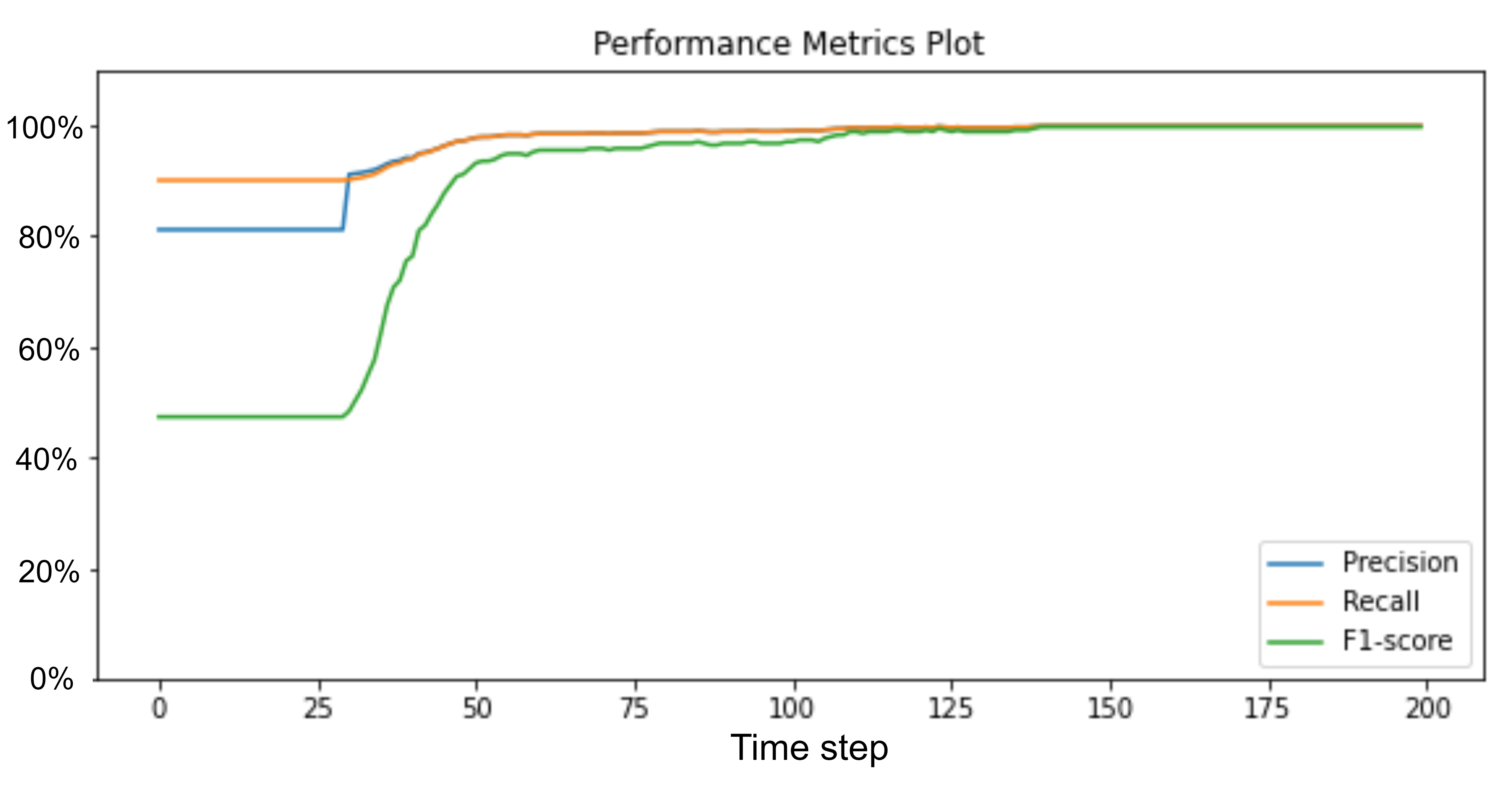
Figure 5: Performance of the safety violation prediction models in the Cart-Pole case study

To answer this research question, we performed a series of $n$ random executions ($n=1000$) of the RL agent and extracted the corresponding episodes $e_{1\leq i\leq n}$. To build our ground truth, these episodes were labeled as either safe or unsafe, taking into account the presence or absence of safety violations observed within each episode. We should note that in both case studies, there was a maximum of one safety violation per episode, occurring at the end of an unsafe episode as part of the termination criteria. We monitored the execution of each episode with SMARLA and at each time step. As described in Section 4.3.2, when the upper bound of the confidence interval $Up(t)$ is greater than 50% during the execution of the episode, SMARLA classifies the episode as unsafe. For each case study, we computed the number of successfully predicted safety violations, measured the prediction precision, recall, and F1-score at each time step, over the set of episodes, and depict the results in Figures 4 and 5.

These figures show a consistent pattern where the precision, recall, and F1-score exhibit a general increase over time before eventually reaching a plateau around 100%. SMARLA’s accuracy is thus improving over time as episodes execute. Ultimately, our safety monitor correctly predicted all 99 and 132 safety violations in the Cart-Pole and Mountain-Car case studies, respectively. We obtained highly accurate safety violation prediction results for both case studies after roughly 50 times steps. In the Cart-Pole case study, we achieved a precision of 98.4%, a recall of 98.4%, and an F1-score of 95%, after time step 59 while in the Mountain-Car case study, we obtained a precision of 99.8%, a recall of 99.8%, and an F1-score of 99.5% after 50 time steps. In both case studies, results highlight SMARLA’s capability to provide accurate predictions of safety violations, relatively early, roughly halfway through the episode’s execution as described next.

In detail, the precision, recall, and F1-score plateau at 98% from time step 106 in Cart-Pole where the average length of the episodes is 193 and the minimum length is 118. At time step 106, on average, 45% of the steps within the episodes remain to execute until reaching an unsafe state. This indicates that there is significant time to apply safety mechanisms.

Similarly, in the Mountain-Car case study, we observed early accurate predictions of safety violations with SMARLA. This is indicated by the precision, recall, and F1-score plateauing from time step 50. The average and minimum episode lengths in this case study are 112 and 95. At this time step, an average of 55% of the steps within the episodes remain to execute. These results further validate the safety violation prediction model’s ability to anticipate safety violations long before they occur.

		Decision time step			Remaining time steps			Remaining % of time steps
Decision criteria	Case study	Min	Avg	Max	Min	Avg	Max	Min	Avg	Max	# FP
	Mountain-Car	15	20.96	38	57	74.21	80	59%	77.16%	83%	2
Upper bound	Cart-Pole	22	41.36	105	67	104.5	164	38.70%	71.35%	82%	11
	Mountain-Car	20	32.53	63	32	62.65	75	33.33%	65.15%	78.12%	1
Output probability	Cart-Pole	30	48.8	126	46	96.48	129	27%	66.58%	78.60%	2
	Mountain-Car	25	44.39	76	19	50.79	70	19.79%	52.81%	72.92%	1
Lower bound	Cart-Pole	33	56.94	171	8	83.36	123	0.49%	61.34%	73.33%	0

Table I: Overview of SMARLA’s decision times and the remaining percentage of time steps before safety violations occur across different decision criteria and case studies (# FP stands for the total number of false positives)

5.4.2 RQ2. How can the safety monitor determine when to trust the prediction of safety violations?

In this research question, we investigate the use of confidence intervals as a means for the safety monitor to determine the appropriate time step to trigger safety mechanisms. This investigation is based on the same set of episodes randomly generated for RQ1 (Section 5.4.1). At each time step $t$, we collect the predicted probability of safety violation $P_{e_{i}}(t)$ and the corresponding confidence interval $[Low(t),Up(t)]$. The lower bound ($Low(t)$) and upper bound ($Up(t)$) of the confidence interval are computed using the methodology detailed in Section 4.3.2.

To determine the best decision criterion for triggering safety mechanisms, we considered and compared the following alternative criteria:

• If the probability of safety violation, $P_{e_{i}}(t)$, is equal to or greater than 50%, then the safety mechanism is activated.

• If the upper bound of the confidence interval at time step $t$ (based on the confidence level of 95%) is above 50% (i.e., $Up(t)\geq 50\%$), then the safety mechanism is activated. This is a conservative approach as the actual probability has a 97.5% chance to be below that value. This may result in many false positives but it leads to early predictions of unsafe episodes and is unlikely to miss any unsafe episodes.

• If the lower bound of the confidence intervals at time step $t$ is above 50% (i.e., $Low(t)\geq 50\%$), then the safety mechanism is activated. In this criterion, the actual probability has only a 2.5% chance to be below that bound and we thus minimize the occurrence of false positives, at the cost of relatively late detection of unsafe episodes and more false negatives.

Decision criteria identify the time step when the execution should be stopped and safety mechanisms should be activated. However, note that during our test, we continue the execution of the episodes until termination in order to extract the number of time steps until termination and the true label of episodes for our analysis.

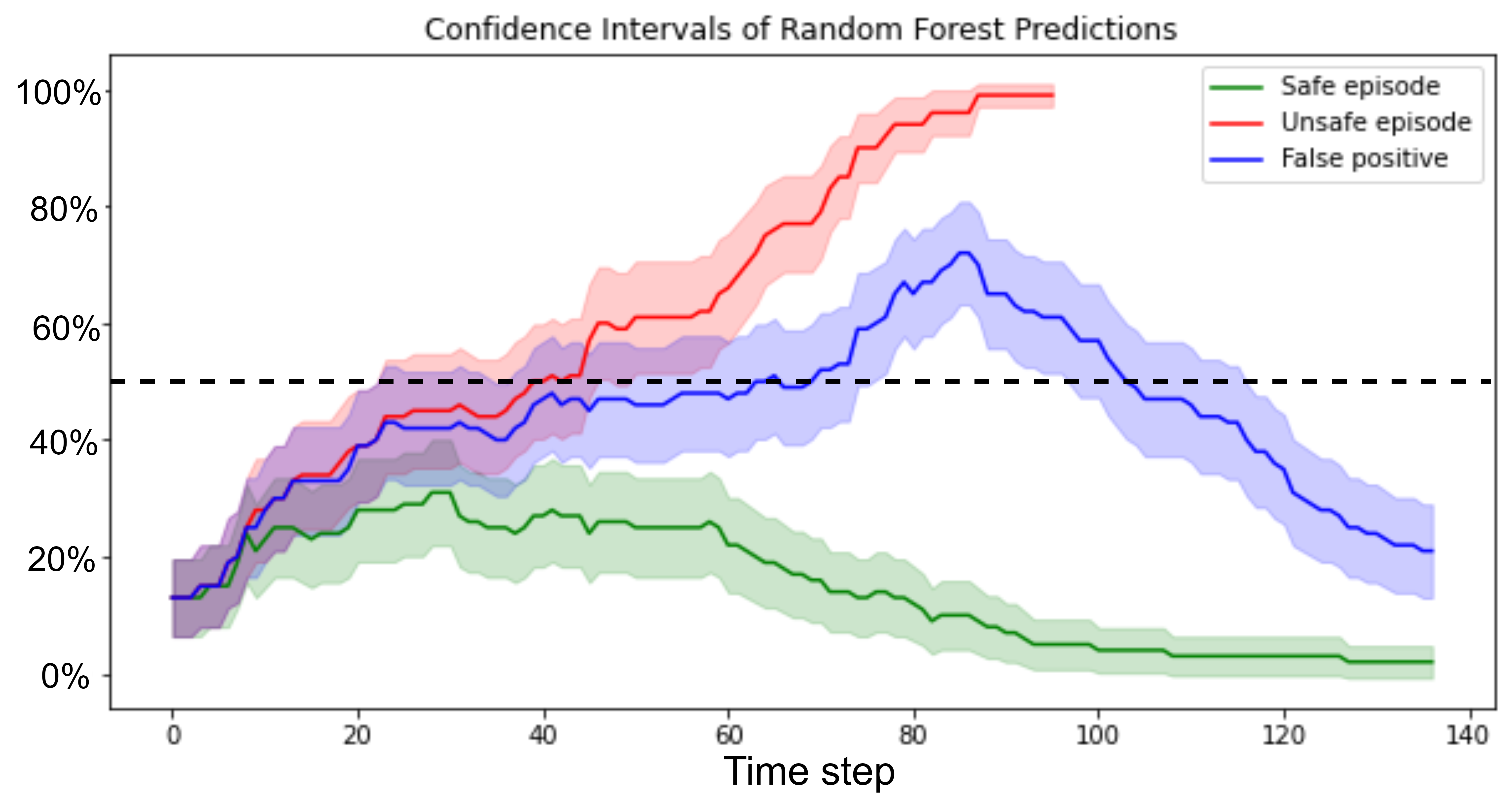
Figure 6: Confidence intervals of a safe episode (in green), an unsafe episode (in red) and a false positive episode (in blue) in the Mountain-Car case study

In Figure 6, we provide representative examples of the estimated probability of safety violation over time for a safe episode, an unsafe episode, and a mispredicted episode (false positive) in the Mountain-Car case study. The curves in the graph represent the output probabilities generated by the safety violation prediction model, while the shaded areas depict the corresponding 95% confidence intervals. We observe that, as more information is acquired, probabilities either tend to increase or decrease depending on whether the episode is safe or unsafe. At some point, the confidence intervals tend to narrow down as enough information from episodes is collected to make an accurate prediction. As expected, in the figure, relying on the upper bound of the confidence interval leads to a much earlier safety violation prediction in the unsafe episode (depicted in red in the figure), compared to when considering the predicted output probability or the lower bound of the confidence interval.

Now the question is how do the predictions based on the three above criteria compare in terms of accuracy. Figures 7 and 8 present a comparison of the F1-scores of the three predictions at each time step for the Mountain-Car and the Cart-Pole case studies, respectively. Though there are differences in the magnitude of the trend, results from our case studies consistently show that using the upper bound is the best choice as it leads to early accurate predictions.

More in detail, we observe that in the Cart-Pole case study, the F1-score based on the upper bound is above 95% from time step 50 and plateaus around 99% at time step 102. On the other hand, when using the output probability of the safety violation prediction model, the F1-score is above 95% starting from time step 59 and reaches its plateau of 99% at time step 135. With the lower bound, however, F1-score is above 95% from time step 99 and reaches a plateau of 98% at time step 150. Similarly, for the Mountain-Car case study, with the upper bound we reach an F1-score above 95% from time step 23 and plateau around 99% at time step 38. In contrast, the F1-score based on the output probability of the safety violation prediction model is above 95% from time step 41 and plateaus around 99% at time step 50. Finally, with the lower bound, the F1-score is above 95% from time step 46, and plateaus around 99% at time step 69.

We also observe that, for all three decision criteria in each case study, the F1-score is low during early steps due to lack of information. It then increases sharply (around time steps 30-40 for Cart-Pole and 15-45 for Mountain-Car) to reach a plateau shortly after 50 time steps. During that time frame, the difference among decision criteria for Mountain-Car is more significant than for Cart-Pole. This discrepancy is due to the wider confidence intervals present in the Mountain-Car case study, which can be explained by wider variance in decision tree predictions. Furthermore, the high F1-scores for all three decision criteria indicate that the confidence intervals significantly narrow once the plateau is reached. At that point, there is no overlap between the confidence intervals of unsafe and safe episodes.

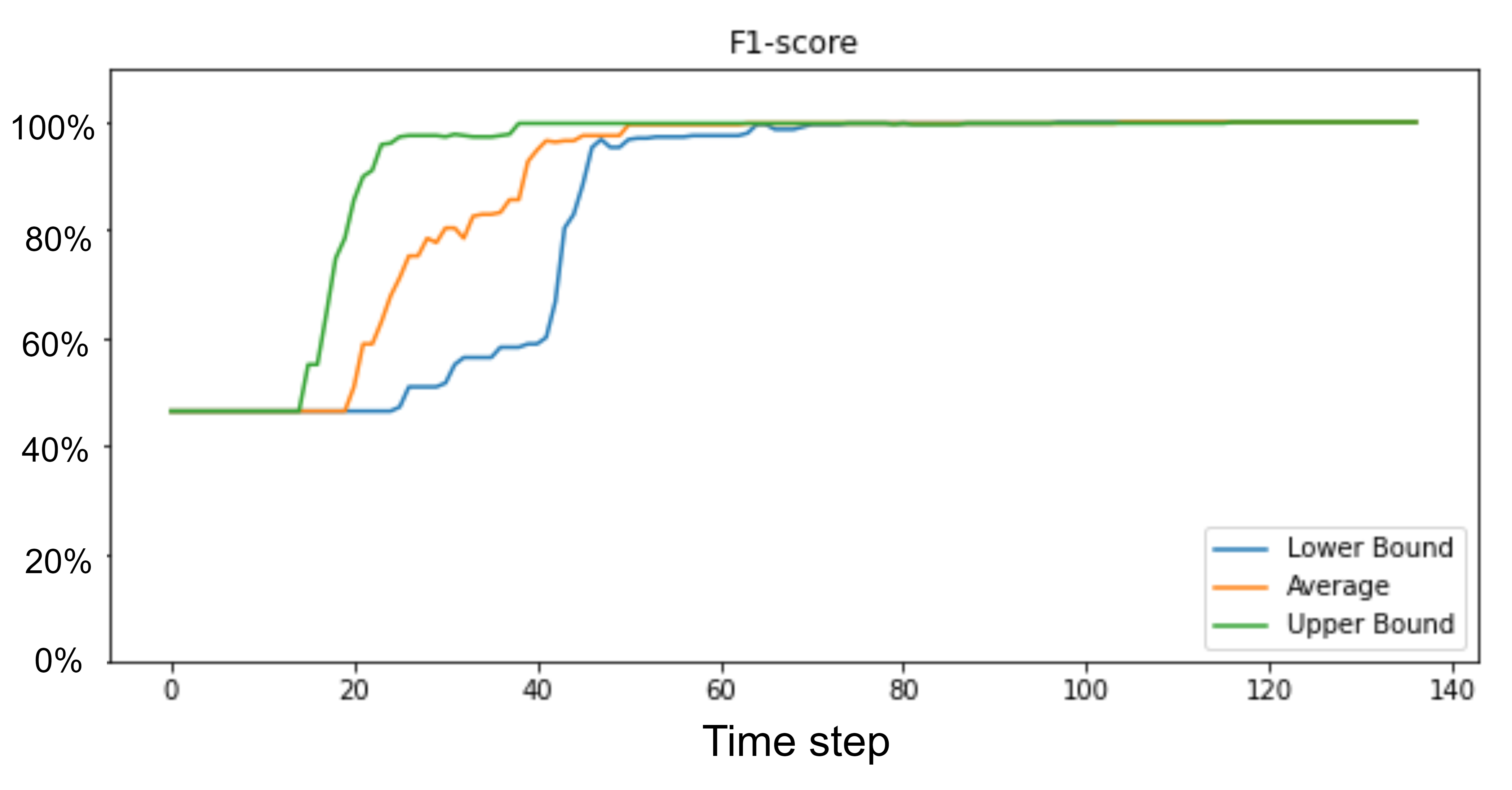
Figure 7: F1-score of the safety violation prediction model for different decision criteria in the Mountain-Car case study

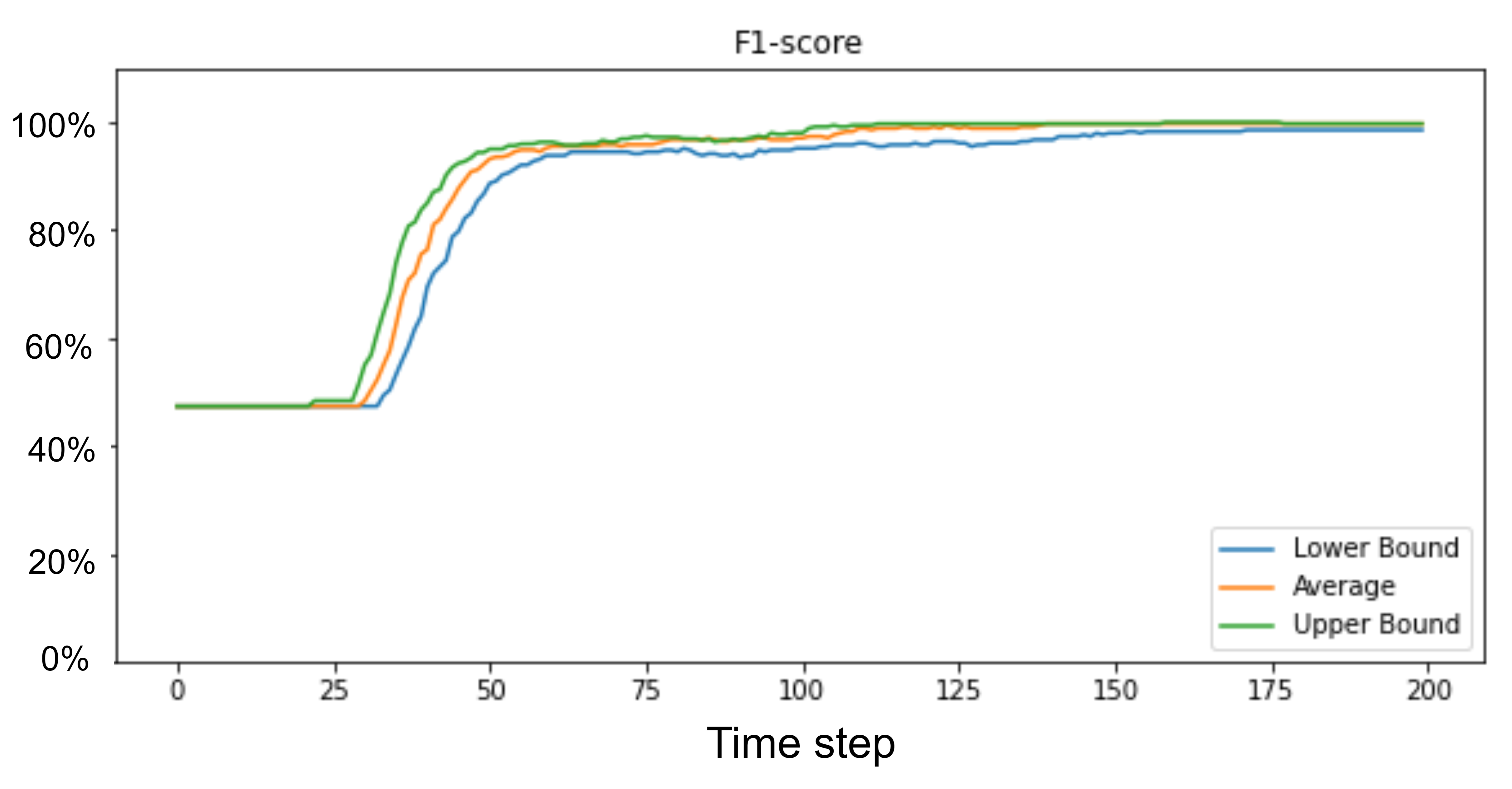
Figure 8: F1-score of the safety violation prediction model for different decision criteria in the Cart-Pole case study

Using these observations, we computed the average improvements, in terms of time steps required to achieve peak performance, when predicting safety violations by considering the upper bound of the confidence interval, in contrast to (1) the output probability and (2) the lower bound of the confidence interval. Our findings indicate that using the upper bound of the confidence intervals results in an average decrease of 24% for both Cart-Pole and Mountain-Car, in terms of time steps required to achieve peak performance, as compared to using the predicted probability. When compared to using the lower bound, the decrease is 32% for Cart-Pole and 45% for Mountain-Car.

We also investigated in both case studies three important metrics: (1) the decision time step, (2) the remaining time steps until the occurrence of a safety violation, and (3) the remaining percentage of time steps to execute until violation. For each metric, we present in Table I the minimum, maximum, and average values. The result in Table I suggests that, relying on the upper bound, the average decision time step in the Mountain-Car case study is 21. However, in the best-case scenario, safety violations are predicted as early as time step 15, while in the worst-case scenario, such violations are predicted at time step 38. Notably, the results demonstrate that when safety mechanisms are triggered, on average 74 times steps (77% ) of episodes remain to be executed. This observation suggests there is ample time to initiate safety mechanisms and hopefully prevent safety violations.

Similarly in the Cart-Pole case study, employing the upper bound, the average prediction time step is determined to be 41. The earliest prediction of a safety violation occurs at time step 22, while the latest prediction is observed at time step 105. Remarkably, on average, there are still 104 time steps remaining to be executed when safety mechanisms are triggered. This accounts for approximately 71% of the average length of episodes, once again suggesting there is significant time available for carrying out safety measures. Overall, the above results demonstrate that SMARLA can predict safety violations early and accurately, suggesting it is a good solution for ensuring system safety when relying on RL agents.

Furthermore, in the Cart-Pole case study, our observations revealed the occurrence of 11 false positives leading to a false positive rate (FPR) of 1%, when relying on the upper bound. In contrast, only two false positives were identified with the output probability ($FPR=0.2\%$), and none when employing the lower bound. Regarding the Mountain-Car case study, two false positives were observed ($FPR=0.2\%$) when employing the upper bound. In contrast, using the output probability or the lower bound resulted in only one false positive ($FPR=0.1\%$).

To summarize, while relying on the upper bound of confidence intervals leads to an earlier prediction of safety violations, it also introduces a higher rate of false positives compared to using the predicted probability and the lower bound. Therefore, considering the trade-off between earlier detection of safety violations and the number of false positives, the selection of an appropriate decision criterion relies heavily on the level of criticality of the RL agent. For instance, in certain scenarios, prioritizing early detection of safety violations and allowing for a longer time frame to apply safety mechanisms may be of critical importance, even at the expense of a slightly higher false positive rate. Conversely, in other cases, there might be a preference to sacrifice time in order to optimize accuracy and minimize the occurrence of false positives. The selection of the appropriate decision criterion depends on the specific context and the relative importance of early detection and prediction accuracy. In our case studies, the increase in false positives appears to be limited, and therefore using the upper bound is the best option.

5.4.3 RQ3. What is the effect of the abstraction level on the safety monitoring system?

To answer this research question, we studied how different levels of state abstraction affect the performance of the safety violation prediction model in the training phase and in operation.

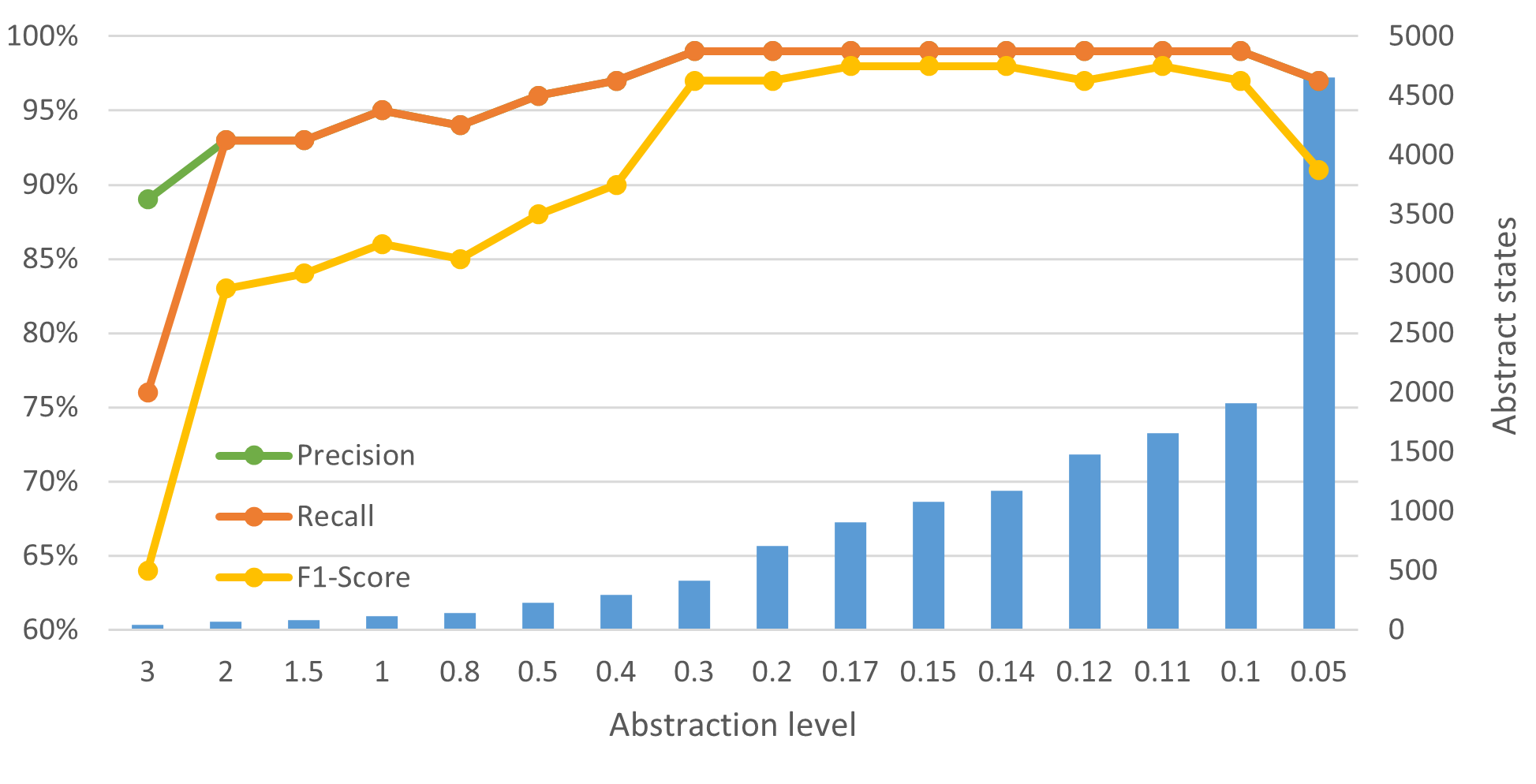
Figure 9: Precision, recall, and F1-score achieved after the training of the safety violation prediction model and the number of abstract states for the Cart-Pole case study across different abstraction levels

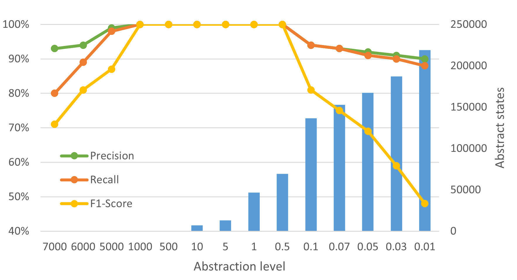
Figure 10: Precision, recall, and F1-score achieved after the training of the safety violation prediction model and the number of abstract states for the Mountain-Car across different abstraction levels

The accuracy of the Random Forest model after training with different abstraction levels. This aspect involves evaluating the performance of the Random Forest model once it has been trained on the available training data. We randomly sampled 70% of the dataset to train and 30% to compute the F1-scores of the models using different levels of abstraction ($d$). A lower abstraction level implies finer-grained states, while higher abstraction levels represent coarser ones that lead to a smaller feature space.

Based on the analysis depicted in Figures 9 and 10, we observed that higher abstraction levels lead to lower accuracy in predicting safety violations, above a threshold of 0.3 for Cart-Pole and 1000 for Mountain-Car. This is attributed to the smaller feature space associated with higher levels of abstraction. As the abstraction level decreases, the feature space grows larger, allowing for more precise information to be captured by features. Consequently, the accuracy of the safety violation prediction model tends to increase until it eventually plateaus and then starts to decrease. This decrease occurs due to the very large number of abstract states, making it more challenging to learn in a larger feature space. This suggests that there is an optimal range of abstraction that yields the highest accuracy in predicting safety violations. Going beyond this optimal range can reduce the performance of safety monitoring. This optimal range of abstraction level depends on the environment, the RL agent, and the reward. This arises from the fact that the calculation of Q-values, which are used in the abstraction process, relies heavily on the reward signal. Consequently, the choice of reward function significantly influences the optimal range of abstraction levels. Indeed, our empirical analysis revealed that abstraction levels ranging from 0.1 to 0.3 result in the highest accuracy for Cart-Pole while for Mountain-Car, abstraction levels from 0.5 to 1000 result in the highest accuracy. Therefore, for the next experiments, we consider the abstraction levels within the optimal ranges of each case study.

The performance of the model in operation with different abstraction levels. This part focuses on evaluating the performance of the safety violation prediction model during the execution of episodes. We analyze how well the trained Random Forest models perform in operation across different time steps while considering different abstraction levels. The main focus for such evaluation is the model’s ability to accurately predict safety violations early.

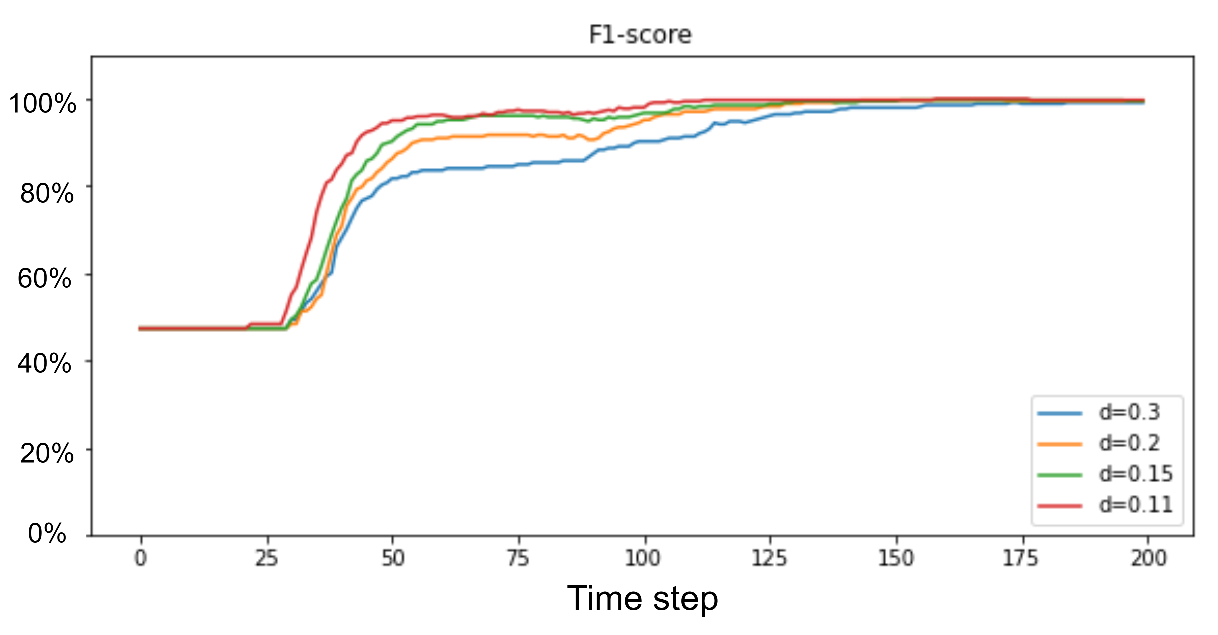
Figure 11: Performance of the safety violation prediction models in operation for the Cart-Pole case study across different levels of abstraction

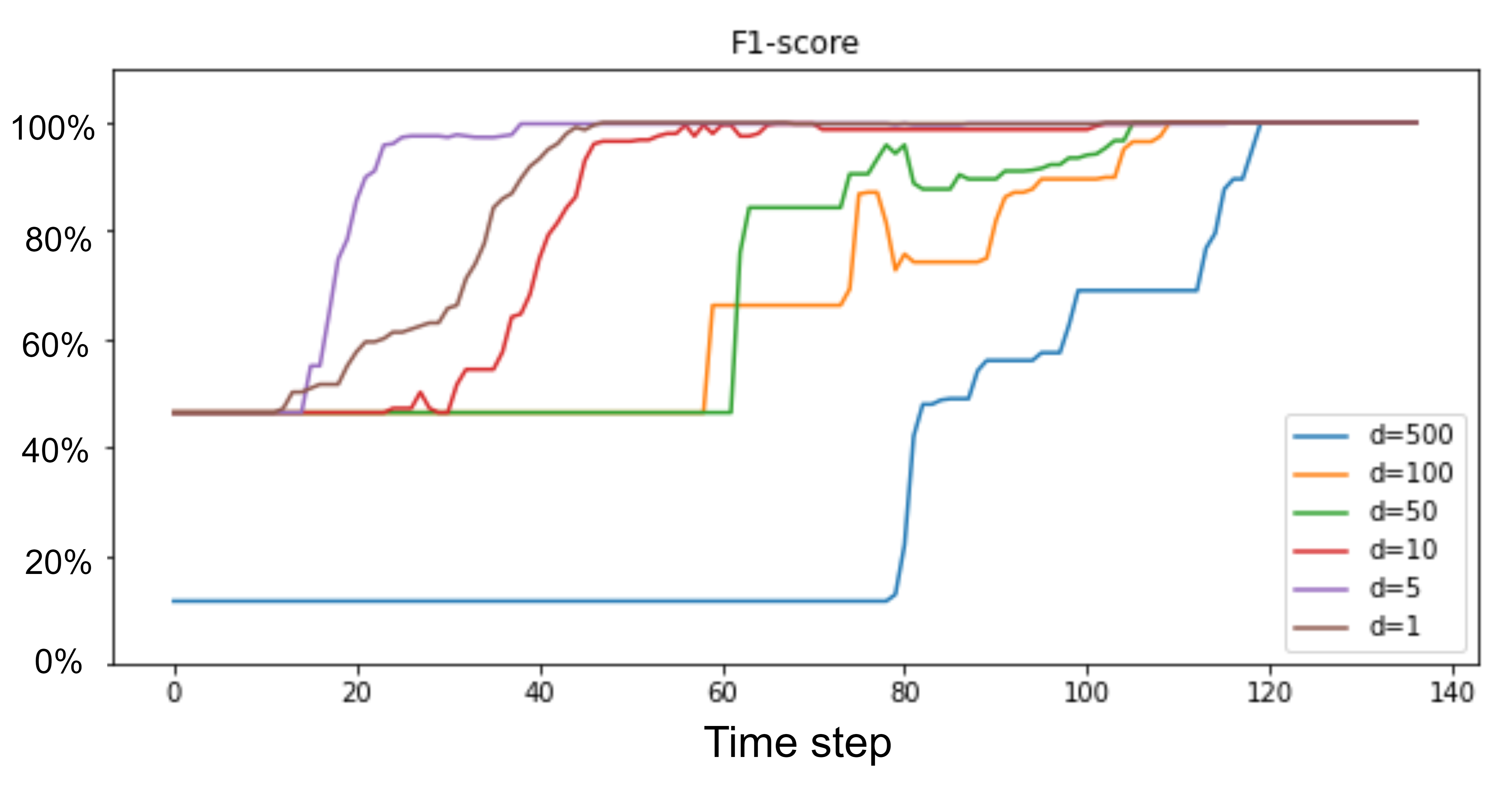
Figure 12: Performance of the safety violation prediction models in operation for the Mountain-Car case study across different levels of abstraction

The F1-score of the safety monitoring models for the two case studies, considering various levels of abstraction, are presented in Figures 11 and 12.

As visible, the performance of the safety violation prediction model is highly sensitive to the selected abstraction level during the training phase, especially in the case of Mountain-Car. Despite selecting only abstraction levels that maximize the model’s performance during training, they required different numbers of time steps to achieve the highest accuracy in predicting safety violations. This sensitivity highlights the importance of carefully selecting the appropriate abstraction level for optimal model performance.

Based on Figures 11 and 12, we observe that the most suitable abstraction level is $d=0.11$ for Cart-Pole and $d=5$ for Mountain-Car, as they exhibit the most accurate and earliest prediction of safety violations compared to other abstraction levels. This indicates that these abstraction levels are particularly effective at capturing relevant features at the right level of granularity to support learning and the prediction of unsafe episodes.

In summary, in this research question, we studied the performance of SMARLA through a systematic two-step process. In the first step, we analyzed the accuracy of SMARLA in predicting safety violations post-training, and we derived a range of optimal abstraction levels corresponding to the highest F1-score. Next, we investigated the number of time steps SMARLA requires to achieve its peak accuracy. Note that, the ultimate objective is to identify the proper abstraction level which enables the safety monitor to reach its highest accuracy in predicting safety violations at the earliest time step possible.

5.4.4 Abstraction level selection procedure

To achieve early and accurate predictions of the safety monitor in practice, it is crucial to determine a proper abstraction level. Thus, based on the results of RQ3 5.4.3, we propose the following procedure to select a proper abstraction level for our monitoring approach. This procedure is a one-time process that involves a systematic two-step approach. Initially, in the first step, a Coarse-to-Fine search technique [42] is used for finding the optimal range of abstraction levels that maximize the F1-score of the safety violation prediction model. Subsequently, in the second step, within this optimal range, the abstraction level yielding the earliest prediction of safety violation is identified.

In detail, this process starts by training the safety violation prediction models with approximately 70% of the training episodes. During this phase, the safety violation prediction model is trained using a diverse range of abstraction levels, systematically varied in increments. The assessment metric is the F1-score of the safety violation prediction model. It is noteworthy that abstraction levels can be mapped to the number of abstract states, thereby facilitating the determination of the range of abstraction levels to be explored. As a practical guideline, using the Coarse-to-Fine approach, it is recommended to start with a wide range spanning from several hundred to approximately 100,000 states. The process involves iteratively considering new values close to abstraction levels that previously yielded high F1-scores, and therefore gradually narrowing down the range to ultimately identify the optimal range of abstraction levels.

However, the choice of the range of levels to cover depends also on the complexity of the environment; more complex environments may necessitate a larger number of abstract states to ensure accurate prediction of safety violations. Subsequently, within the recommended range, the optimal subset of abstraction levels can be determined by selecting levels that maximize the F1-score of the models when evaluated on the remaining 30% of episodes. The results of this step for the Cart-Pole and the Mountain-Car case studies are depicted in Figures 9 and 10, respectively. In the Cart-Pole case study, the optimal range of abstraction levels lies between 0.1 and 0.3, whereas for the Mountain-Car, it is between 0.5 and 1000.

In the second phase, it is imperative to conduct experiments with different abstraction levels within the optimal range when utilizing the safety violation prediction model during the execution of the episode. The primary objective is to pinpoint the level of abstraction that enables the safety monitor to make precise predictions of safety violations at the earliest time step possible. Figures 11 and 12 illustrate the outcomes of the second phase, where we extracted the F1-score of safety monitoring models considering various abstraction levels within the optimal range. As a result, the optimal abstraction levels that enable accurate and early predictions of the safety monitoring approach for the Cart-Pole and Mountain-Car case studies are $d=0.11$ and $d=5$, respectively.

6 Threats to Validity

In this section, we discuss the different threats to the validity of our study and describe how we mitigated them.

Internal threats concern the causal relationship between the treatment and the outcome. One such threat is the choice of an inappropriate state abstraction level. To mitigate this threat, we explored different abstraction levels and identified the ones that (1) significantly reduce the state space, (2) optimize the accuracy of the ML model, and (3) enable the earliest and most accurate predictions of safety violations during the RL agent execution. Another threat pertains to newly seen abstract states during operation (i.e., abstract states that were not included in the training dataset of the safety violation prediction model), which may impact the accuracy of the safety monitoring system. To mitigate the risk of missing abstract states, we trained our ML model with a large and diverse dataset of RL episodes and use a state abstraction method that considers a large number of concrete states (roughly 450 000 in Cart-Pole and 250 000 in Mountain-Car). We will study, in future work, the impact of retraining the ML model (to include newly seen abstract states) on the performance of our safety monitoring approach. The scarcity of unsafe episodes poses a threat to accurate safety violation model training. As future work, we will explore extracting unsafe episodes from the later stages of the RL agent’s training phase, as they align more closely with the agent’s final policy.

Conclusion threats are concerned with the relationship between treatment and outcome. One important threat to consider is the potential impact of a large monitor’s overhead on its applicability in real-time scenarios. Such overhead refers to the additional computational resources and time required by safety monitoring. To mitigate this threat, SMARLA relies on state abstraction to reduce the state space and computation overhead. It also uses Random Forest, which is a lightweight machine learning model known for its fast inference capabilities [31, 43]. This choice helps minimize the computational burden associated with monitoring, allowing for fast processing and response times. Note that, in our case studies, inference times (i.e., safety violation predictions) are in the range of a few milliseconds, thus confirming our expectations. Finally, our monitoring approach is black-box. It does not require access to the internals of the RL agent, which greatly simplifies processing and reduces computation overhead.

Reliability threats concern the replicability of our study results. We rely on publicly available ML models and RL environments. We provide online all the materials required to replicate our study results.

External threats concern the generalizability of our study. Due in part to the high computational expense of our experiments, we relied on two case studies in our work, which may threaten the generalizability of our results. Indeed, experiments for all research questions took about two weeks using a system with a Core-i9 processor, 32GB of memory, and an Nvidia GeForce RTX 3070 GPU with 8GB of memory. However, to mitigate this threat, we relied on benchmark problems widely used in many RL-related studies [34, 35, 36, 37]. Future work includes applying our monitoring approach to different RL problems for broader generalization of the results.

7 Related Work

This section provides an overview of the most relevant literature on safety monitors. We discuss related works on (1) safety monitors for RL agents, and (2) safety monitors for AI/ML-based systems in general. Other less closely related aspects are left out, due to space constraints.

7.1 Safety monitors for RL

Several approaches have been proposed in the literature on safe reinforcement learning [44, 45, 46], but only a few of them proposed safety monitors to predict safety violations of the agent at runtime. Junges et al. [47] proposed two strategies for monitoring MDPs: forward filtering-based monitoring and model checking-based monitoring. The former involves estimating future possible states of the system based on historical observations. In contrast, the latter uses model-checking techniques to assess the probability of reaching certain states in the MDP. These strategies are only applicable when a detailed model of the environment is available, in contrast to SMARLA which works on a broader type of model-free RL algorithms which are more widely used in practice as environment models are challenging to develop and validate [48, 49].

Other approaches have been proposed for the online safety shielding of RL agents where a shield layer is added to the agent and blocks unsafe actions during the execution [18, 50]. In general, online shielding operates by dynamically calculating, during runtime, the collection of potential states that may be reached in the immediate future. Within this set of states, the safety of all feasible actions is assessed and leveraged for shielding purposes as soon as any of the aforementioned states is encountered. In that context, Konighofer et al. [18] proposed an online shielding technique for RL agents that employs MDPs and probabilistic model-checking to evaluate all possible actions in the agent’s states. By blocking unsafe actions and analyzing the impact of shielding on learning performance and policy safety, they demonstrate improved learning performance with shielding and recommend its application during both the training and execution phases of RL agents. Other shielding approaches have been proposed to increase the safety of RL agents during the training phase [51, 17]. For example, Mallozzi et al. [51] introduced WiseML, a runtime safety monitoring framework for RL agents. The goal of this framework is to prevent the agent from selecting unsafe actions during training by relying on manual specifications of safety violation patterns using linear-time temporal logic. The monitoring system blocks safety violations, penalizes the agent’s reward for unsafe actions, and enhances the learning performance of the agent by accelerating the convergence to its goal. Also, Elsayed et al. [17] proposed a shielding approach for multi-agent reinforcement learning. Their goal is to enforce safety specifications expressed in linear temporal logic and learn safe RL policies in multi-agent environments.

Our research objectives differ from shielding-based studies as we propose a black-box safety monitor for RL agents that does not force the agent to select non-optimal actions (i.e., actions that deviate from the optimal policy) and continue the execution relying on the policy of the agent. Rather, our focus is on the early prediction of safety violations to provide engineers with the flexibility to implement a range of safety mechanisms, including the option to apply early corrective or preventive safety measures.

7.2 Safety monitors for AI/ML

Different approaches have been proposed in the literature to monitor the safety of ML-based systems due to concerns about their reliability, especially in safety-critical systems [52, 53, 54, 55, 56]. Some studies focus on detecting distributional shift (between training inputs and data seen in operation time) [52, 53, 54, 55] resulting in DNN mispredictions during operation [56, 57], aiming to maintain accuracy and reduce safety risks. These approaches compare neurons activation patterns [52, 53] or features distributions [54] of inputs during operation with those seen during training. Other approaches involve monitoring DNN outputs and verifying their confidence levels to predict DNNs mispredictions [58]. Furthermore, Stocco et al. [56] introduced SafeOracle, an unsupervised monitoring tool for autonomous driving systems. SafeOracle aims to predict a DNN’s misbehavior by building a proxy for the DNN’s output confidence level at runtime. The authors have proposed an autoencoder-based image reconstruction technique to forecast the subsequent input images. Additionally, they have trained an anomaly detector on the nominal image inputs of the DNN, which observes the reconstruction error to identify any anomaly. In their approach, they combine confidence estimation, probability distribution fitting, and time series analysis, and show that they were able to identify 77% of safety violations up to six seconds in advance. In contrast, our work specifically addresses safety monitoring for DRL agents and relies on ML models and state abstraction to predict safety violations during operation. More precisely, we monitor the behavior and state information of the agents to predict violations in all conditions, as opposed to relying solely on out-of-distribution inputs.

Overall, SMARLA stands out by providing a novel safety monitoring approach that is black-box and tailored for RL agents, and prioritizes the early prediction of safety violations, thus providing the flexibility to implement a wide range of safety mechanisms. The use of state abstraction and ML models allows for efficient and accurate safety violation prediction, without requiring detailed environment models, making it well-suited for a broader range of model-free RL algorithms that are commonly used.

8 Conclusion

In this paper, we propose SMARLA, a black-box safety monitoring approach for reinforcement learning agents. We rely on a machine learning model to predict safety violations of RL agents early during their execution. We employ state abstraction to reduce the state space, enabling improved learnability for predicting violations. We evaluate our safety monitoring approach on two widely used RL benchmarks. Our results demonstrate the high accuracy of SMARLA in predicting the safety violations of RL agents during their execution. Additionally, our empirical results show that such accurate prediction can be made early long before the actual occurrence of violations, allowing for timely damage prevention and mitigation. In future work, we intend to expand our evaluation to include additional RL case studies. Additionally, to further improve accuracy and early predictions, we aim to investigate the use of other types of features that consider temporal information regarding the agent’s states and actions in RL episodes. For instance, we can consider the sequence of abstract states instead of only considering their presence or absence as features.

References

- [1] L. Meng, R. Gorbet, and D. Kulić, “Memory-based deep reinforcement learning for pomdps,” in 2021 IEEE/RSJ International Conference on Intelligent Robots and Systems (IROS). IEEE, 2021, pp. 5619–5626.
- [2] K. Arulkumaran, M. P. Deisenroth, M. Brundage, and A. A. Bharath, “Deep reinforcement learning: A brief survey,” IEEE Signal Processing Magazine, vol. 34, no. 6, pp. 26–38, 2017.
- [3] M. Turchetta, A. Kolobov, S. Shah, A. Krause, and A. Agarwal, “Safe reinforcement learning via curriculum induction,” Advances in Neural Information Processing Systems, vol. 33, pp. 12 151–12 162, 2020.
- [4] G. Dulac-Arnold, N. Levine, D. J. Mankowitz, J. Li, C. Paduraru, S. Gowal, and T. Hester, “Challenges of real-world reinforcement learning: definitions, benchmarks and analysis,” Machine Learning, vol. 110, no. 9, pp. 2419–2468, 2021.
- [5] M. Alshiekh, R. Bloem, R. Ehlers, B. Könighofer, S. Niekum, and U. Topcu, “Safe reinforcement learning via shielding,” in Proceedings of the AAAI Conference on Artificial Intelligence, vol. 32, no. 1, 2018.
- [6] “Road vehicles – functional safety,” ISO 26262:2018, 2018.
- [7] “Road vehicles — safety of the intended functionality,” ISO/PAS 21448:2019, 2019.
- [8] G. Dulac-Arnold, D. Mankowitz, and T. Hester, “Challenges of real-world reinforcement learning,” 2019.
- [9] K. Hansen, A. Ravn, and V. Stavridou, “From safety analysis to software requirements,” IEEE Transactions on Software Engineering, vol. 24, no. 7, pp. 573–584, 1998.
- [10] E. Marchesini, L. Marzari, A. Farinelli, and C. Amato, “Safe deep reinforcement learning by verifying task-level properties,” in Proceedings of the 2023 International Conference on Autonomous Agents and Multiagent Systems, 2023, pp. 1466–1475.
- [11] G. Katz, C. Barrett, D. L. Dill, K. Julian, and M. J. Kochenderfer, “Reluplex: An efficient smt solver for verifying deep neural networks,” in Computer Aided Verification: 29th International Conference, CAV 2017, Heidelberg, Germany, July 24-28, 2017, Proceedings, Part I 30. Springer, 2017, pp. 97–117.
- [12] A. Zolfagharian, M. Abdellatif, L. C. Briand, M. Bagherzadeh, and S. Ramesh, “A search-based testing approach for deep reinforcement learning agents,” IEEE Transactions on Software Engineering, 2023.
- [13] Z. Aghababaeyan, M. Abdellatif, L. Briand, S. Ramesh, and M. Bagherzadeh, “Black-box testing of deep neural networks through test case diversity,” IEEE Transactions on Software Engineering, 2023.
- [14] Z. Aghababaeyan, M. Abdellatif, M. Dadkhah, and L. Briand, “Deepgd: A multi-objective black-box test selection approach for deep neural networks,” 2024.
- [15] M. Pecka and T. Svoboda, “Safe exploration techniques for reinforcement learning–an overview,” in Modelling and Simulation for Autonomous Systems: First International Workshop, MESAS 2014, Rome, Italy, May 5-6, 2014, Revised Selected Papers 1. Springer, 2014, pp. 357–375.
- [16] Y. Okawa, T. Sasaki, H. Yanami, and T. Namerikawa, “Safe exploration method for reinforcement learning under existence of disturbance,” 2023.
- [17] I. ElSayed-Aly, S. Bharadwaj, C. Amato, R. Ehlers, U. Topcu, and L. Feng, “Safe multi-agent reinforcement learning via shielding,” arXiv preprint arXiv:2101.11196, 2021.
- [18] B. Könighofer, J. Rudolf, A. Palmisano, M. Tappler, and R. Bloem, “Online shielding for reinforcement learning,” Innovations in Systems and Software Engineering, pp. 1–16, 2022.
- [19] D. Abel, D. Arumugam, L. Lehnert, and M. Littman, “State abstractions for lifelong reinforcement learning,” in Proceedings of the 35th International Conference on Machine Learning, ser. Proceedings of Machine Learning Research, J. Dy and A. Krause, Eds., vol. 80. PMLR, 10–15 Jul 2018, pp. 10–19. [Online]. Available: http://proceedings.mlr.press/v80/abel18a.html
- [20] N. Jiang, “Notes on state abstractions,” 2018.
- [21] L. Li, T. J. Walsh, and M. L. Littman, “Towards a unified theory of state abstraction for mdps.” ISAIM, vol. 4, no. 5, p. 9, 2006.
- [22] B. Jang, M. Kim, G. Harerimana, and J. W. Kim, “Q-learning algorithms: A comprehensive classification and applications,” IEEE access, vol. 7, pp. 133 653–133 667, 2019.
- [23] R. S. Sutton and A. G. Barto, Reinforcement learning: An introduction. MIT press, 2018.
- [24] R. Akrour, F. Veiga, J. Peters, and G. Neumann, “Regularizing reinforcement learning with state abstraction,” in 2018 IEEE/RSJ International Conference on Intelligent Robots and Systems (IROS). IEEE, 2018, pp. 534–539.
- [25] S. Hao, L. Li, M. Liu, Y. Zhu, and D. Zhao, “Learning representation with q-irrelevance abstraction for reinforcement learning,” in 2021 11th International Conference on Intelligent Control and Information Processing (ICICIP). IEEE, 2021, pp. 367–373.
- [26] M. Liu, L. Li, S. Hao, Y. Zhu, and D. Zhao, “Soft contrastive learning with q-irrelevance abstraction for reinforcement learning,” IEEE Transactions on Cognitive and Developmental Systems, 2022.
- [27] Y. Tang and S. Agrawal, “Discretizing continuous action space for on-policy optimization,” in Proceedings of the aaai conference on artificial intelligence, vol. 34, no. 04, 2020, pp. 5981–5988.
- [28] A. Tavakoli, F. Pardo, and P. Kormushev, “Action branching architectures for deep reinforcement learning,” in Proceedings of the aaai conference on artificial intelligence, vol. 32, no. 1, 2018.
- [29] P. Swazinna, S. Udluft, D. Hein, and T. Runkler, “Comparing model-free and model-based algorithms for offline reinforcement learning,” arXiv preprint arXiv:2201.05433, 2022.
- [30] “Openai,” https://spinningup.openai.com/en/latest/spinningup/rl_intro2.html, 2018, [Accessed 24 Jan. 2022.].
- [31] L. Breiman, “Random forests,” Mach. Learn., vol. 45, no. 1, p. 5–32, Oct. 2001. [Online]. Available: https://doi.org/10.1023/A:1010933404324
- [32] J. H. Friedman, “Greedy function approximation: a gradient boosting machine,” Annals of statistics, pp. 1189–1232, 2001.
- [33] V. J. Easton and J. H. McColl, “Statistics glossary v1. 1,” 1997.
- [34] V. Behzadan and W. H. Hsu, “Adversarial exploitation of policy imitation,” ArXiv, vol. abs/1906.01121, 2019.
- [35] V. Behzadan and W. Hsu, “Sequential triggers for watermarking of deep reinforcement learning policies,” ArXiv, vol. abs/1906.01126, 2019.
- [36] K. Chen, T. Zhang, X. Xie, and Y. Liu, “Stealing deep reinforcement learning models for fun and profit,” CoRR, vol. abs/2006.05032, 2020. [Online]. Available: https://arxiv.org/abs/2006.05032
- [37] A. Pattanaik, Z. Tang, S. Liu, G. Bommannan, and G. Chowdhary, “Robust deep reinforcement learning with adversarial attacks,” in Proceedings of the 17th International Conference on Autonomous Agents and MultiAgent Systems, 2018, pp. 2040–2042.
- [38] A. Hill, A. Raffin, M. Ernestus, A. Gleave, A. Kanervisto, R. Traore, P. Dhariwal, C. Hesse, O. Klimov, A. Nichol, M. Plappert, A. Radford, J. Schulman, S. Sidor, and Y. Wu, “Stable baselines,” https://github.com/hill-a/stable-baselines, 2018.
- [39] V. Mnih, K. Kavukcuoglu, D. Silver, A. Graves, I. Antonoglou, D. Wierstra, and M. Riedmiller, “Playing atari with deep reinforcement learning,” arXiv preprint arXiv:1312.5602, 2013.
- [40] H. van Hasselt, A. Guez, and D. Silver, “Deep reinforcement learning with double q-learning,” 2015.
- [41] Z. Wang, T. Schaul, M. Hessel, H. van Hasselt, M. Lanctot, and N. de Freitas, “Dueling network architectures for deep reinforcement learning,” 2016.
- [42] J. Schaeffer, N. Sturtevant, R. Holte, and K. Anderson, “Coarse-to-fine search techniques,” 2008.
- [43] J. Cao, Z. Guo, Y. Lv, M. Xu, C. Huang, and H. Liang, “Pollution risk prediction for cadmium in soil from an abandoned mine based on random forest model,” International Journal of Environmental Research and Public Health, vol. 20, no. 6, p. 5097, Mar 2023. [Online]. Available: http://dx.doi.org/10.3390/ijerph20065097
- [44] P. S. N. Mindom, A. Nikanjam, F. Khomh, and J. Mullins, “On assessing the safety of reinforcement learning algorithms using formal methods,” in 2021 IEEE 21st International Conference on Software Quality, Reliability and Security (QRS). IEEE, 2021, pp. 260–269.
- [45] S. Gu, L. Yang, Y. Du, G. Chen, F. Walter, J. Wang, Y. Yang, and A. Knoll, “A review of safe reinforcement learning: Methods, theory and applications,” arXiv preprint arXiv:2205.10330, 2022.
- [46] J. Garcıa and F. Fernández, “A comprehensive survey on safe reinforcement learning,” Journal of Machine Learning Research, vol. 16, no. 1, pp. 1437–1480, 2015.
- [47] S. Junges, H. Torfah, and S. A. Seshia, “Runtime monitors for markov decision processes,” in Computer Aided Verification: 33rd International Conference, CAV 2021, Virtual Event, July 20–23, 2021, Proceedings, Part II. Springer, 2021, pp. 553–576.
- [48] H.-n. Wang, N. Liu, Y.-y. Zhang, D.-w. Feng, F. Huang, D.-s. Li, and Y.-m. Zhang, “Deep reinforcement learning: a survey,” Frontiers of Information Technology & Electronic Engineering, vol. 21, no. 12, pp. 1726–1744, 2020.
- [49] F. Semeraro, A. Griffiths, and A. Cangelosi, “Human–robot collaboration and machine learning: A systematic review of recent research,” Robotics and Computer-Integrated Manufacturing, vol. 79, p. 102432, 2023.
- [50] D. Melcer, C. Amato, and S. Tripakis, “Shield decentralization for safe multi-agent reinforcement learning,” Advances in Neural Information Processing Systems, vol. 35, pp. 13 367–13 379, 2022.
- [51] P. Mallozzi, E. Castellano, P. Pelliccione, G. Schneider, and K. Tei, “A runtime monitoring framework to enforce invariants on reinforcement learning agents exploring complex environments,” in 2019 IEEE/ACM 2nd International Workshop on Robotics Software Engineering (RoSE). IEEE, 2019, pp. 5–12.
- [52] C.-H. Cheng, G. Nührenberg, and H. Yasuoka, “Runtime monitoring neuron activation patterns,” in 2019 Design, Automation & Test in Europe Conference & Exhibition (DATE). IEEE, 2019, pp. 300–303.
- [53] T. A. Henzinger, A. Lukina, and C. Schilling, “Outside the box: Abstraction-based monitoring of neural networks,” arXiv preprint arXiv:1911.09032, 2019.
- [54] K. Aslansefat, I. Sorokos, D. Whiting, R. Tavakoli Kolagari, and Y. Papadopoulos, “Safeml: safety monitoring of machine learning classifiers through statistical difference measures,” in Model-Based Safety and Assessment: 7th International Symposium, IMBSA 2020, Lisbon, Portugal, September 14–16, 2020, Proceedings 7. Springer, 2020, pp. 197–211.
- [55] R. S. Ferreira, J. Arlat, J. Guiochet, and H. Waeselynck, “Benchmarking safety monitors for image classifiers with machine learning,” in 2021 IEEE 26th Pacific Rim International Symposium on Dependable Computing (PRDC). IEEE, 2021, pp. 7–16.
- [56] A. Stocco, M. Weiss, M. Calzana, and P. Tonella, “Misbehaviour prediction for autonomous driving systems,” in Proceedings of the ACM/IEEE 42nd international conference on software engineering, 2020, pp. 359–371.
- [57] A. Stocco, P. J. Nunes, M. D’Amorim, and P. Tonella, “Thirdeye: Attention maps for safe autonomous driving systems,” in Proceedings of the 37th IEEE/ACM International Conference on Automated Software Engineering, 2022, pp. 1–12.
- [58] M. Weiss and P. Tonella, “Fail-safe execution of deep learning based systems through uncertainty monitoring,” in 2021 14th IEEE Conference on Software Testing, Verification and Validation (ICST). IEEE, 2021, pp. 24–35.