Rios and Torrico Platform Design in Matching Markets Platform Design in Matching Markets:
A Two-Sided Assortment Optimization Approach

Ignacio Rios School of Management, University of Texas at Dallas, ignacio.riosuribe@utdallas.edu Alfredo Torrico CDSES, Cornell University, alfredo.torrico@cornell.edu

Motivated by online dating apps, we consider the assortment optimization problem faced by a two-sided matching platform. Users on each side observe an assortment of profiles and decide which of them to like. A match occurs if and only if two users mutually like each other, potentially in different periods. We study how platforms should make assortment decisions to maximize the expected number of matches under different platform designs, varying (i) how users interact with each other, i.e., whether one or both sides of the market can initiate an interaction, and (ii) the timing of matches, i.e., either sequentially or also simultaneously. We show that the problem is NP-hard and that common approaches perform arbitrarily badly. Given the complexity of the problem and industry practices, we focus on the case with two periods and provide algorithms and performance guarantees for different platform designs. We establish that, when interactions are one-directional and matches only take place sequentially, there is an approximation guarantee of $1-1/e$, which becomes arbitrarily close to $1/2$ if we allow for two-directional interactions. Moreover, when we enable matches to happen sequentially and simultaneously in the first period, we provide an approximation guarantee close to $1/2$, which becomes approximately $1/3$ when we allow two-directional interactions. Finally, we discuss some model extensions and use data from our industry partner to numerically show that the loss for not considering simultaneous matches is negligible. Our results suggest that platforms should focus on simple sequential adaptive policies to make assortment decisions.

Two-sided Assortment Optimization, Matching Markets, Submodular Optimization.

1 Introduction

A common feature of many matching platforms is their two-sided design, in which (i) both sides of the market have preferences, (ii) both sides of the market can initiate an interaction with the other side, and (iii) users must mutually agree to generate a match. Examples include freelancing platforms such as TaskRabbit or UpWork, ride-sharing apps such as Blablacar, accommodation companies such as Airbnb, and dating platforms such as Hinge and Bumble. In many of these platforms, the path toward a match starts with the platform eliciting preferences on both sides of the market. For instance, most dating platforms require users to provide basic information such as their age, height, location, religion, and race, among others, and also to report their preferences over these attributes. After collecting this information, most of these platforms display a limited set of alternatives that users can screen before interacting with the other side of the market. Depending on the setting, this interaction can be one-directional, with one side of the market sending an initial request/message/like and the other side of the market either accepting or rejecting it; or it can be two-directional, with both sides of the market being able to screen alternatives and move first. Airbnb, Blablacar, and Bumble are examples of the former, while Hinge and Upwork are examples of the latter. Finally, in all these platforms, a transaction or a match takes place if, and only if, both sides of the market mutually accept/like each other.

As the previous discussion illustrates, one of the primary roles of these platforms is to select the subset of alternatives—the assortment—to display, considering the preferences and characteristics of the users on both sides of the market. We refer to this problem as a two-sided assortment problem. While similar to the traditional (one-sided) assortment optimization problem faced by retailers, where they decide which products to display to maximize expected revenue from customers, the two-sided nature introduces additional complexities. Notably, in the two-sided problem, both users need to acknowledge and agree with each other mutually. Therefore, even if one user expresses interest in another, there is uncertainty regarding whether a match will actually occur. Furthermore, the platform must carefully balance relevance by showing options likely to result in a match, and congestion, as highly popular users may receive more requests than they can handle.

By carefully choosing the timing by which users can interact and the assortments to display, platforms can influence the matching process and balance the trade-off between relevance and congestion. Our research aims to guide platforms on how to make these decisions. More specifically, the goal of this paper is twofold. First, we provide a framework to make optimal two-sided assortment decisions under different platform designs, i.e., varying the constraints on how users interact with each other and how matches are formed. Second, we study the effectiveness of commonly used algorithms, design near-optimal ones, and analyze their performance in theory and practice.

1.1 Contributions

We study how platforms should make two-sided assortment decisions and how the timing in which users interact affects the design of algorithms and their performance. To this end, we first provide a stylized model of a two-sided market mediated by a platform. The platform must choose which subset of profiles (i.e., the assortment) to show to each user. Then, users decide whether to like or dislike each option in their assortments. The novelty of our work is that we allow the platform to impose different constraints on how users interact with each other and how they can form matches. We consider platform designs that vary (i) which side of the market can reach out first, allowing it to be one-directional—where one side evaluates first and the second only observes users that previously liked them—or two-directional—where both sides of the market can see and evaluate new users in each period; and (ii) how matches can be formed, allowing them to be sequential—whereby users see and like each other in different periods after observing an initial like—or simultaneous—whereby users can see and like each other in the same period.

First, we show that the problem faced by the platform is NP-hard, even if we consider the simplest case with a time horizon of two periods and a platform design that only allows one-directional interactions and sequential matches. Thus, to facilitate the theoretical analysis, we focus on the two-period version of the problem where the platform chooses the assortments to show in the first period and, based on users’ decisions, decides the second-period assortments to maximize the expected number of matches from interactions initiated in the first period. This case is relevant in practice since one-lookahead policies perform well, so this assumption is without major practical loss (see Rios et al. (2023)). Moreover, the two-period version of the problem is theoretically interesting and challenging, as we show that many common approaches (such as greedy, perfect matching, and any non-adaptive deterministic approach) can perform arbitrarily poorly in this setting.

Despite these negative results, we provide constant factor approximations for each variant of the problem, as summarized in Table 2. The first variant of the problem is when we only allow for one-directional interactions and sequential matches, i.e., only users on one side of the market can initiate an interaction and no pair of users see each other in the same period. This case is particularly interesting because many two-sided marketplaces operate in this way, motivating recent work (Ashlagi et al. 2022, Aouad and Saban 2022, Torrico et al. 2021). Moreover, some major dating apps (e.g., Bumble) only allow one side of the market to reach out first, which has been shown to improve the overall social welfare Kanoria and Saban (2021), Immorlica et al. (2022). In this case, we provide an algorithm with a performance guarantee of $1-1/e$.

The second variant of the problem extends the first one by allowing sequential matches to happen in both directions, i.e., two-directional sequential matches. In this case, the platform selects assortments for users on both sides of the market in each period and, thus, both sides of the market can initiate an interaction. However, we assume that no pair of users see each other in the same period, so matches can only occur in the second period. This design matches dating platforms that select users’ assortments dynamically over time (e.g., Tinder), responding to users’ like and dislike decisions. In this case, we provide a performance guarantee arbitrarily close to $1/2$ using algorithmic tools from submodular maximization.

The third variant expands on the initial one by allowing simultaneous matches in the first period. More precisely, the platform chooses assortments for the “initiating” side of the market (hence, one-directional interactions) but can also select pairs of users that will see each other in the first period and, thus, matches can happen if both users in these pairs see and like each other. This design is used in some dating apps that combine “standard swiping” with video speed dating, such as Filteroff and The League, where users can evaluate profiles as usual but can also log in at specific times and get matched with users in their assortment for short video speed dates. For this setting, we provide a performance guarantee close to $1/2$.

The last variant of the problem is when interactions are two-directional, and matches can happen either (i) sequentially or (ii) simultaneously in the first period. This platform design captures the one used by many dating apps, such as Hinge and Coffee Meets Bagel, that daily precompute (generally in the middle of the night) the assortments to display in a given day and do not adjust them based on users’ activity during the same day. In this case, we provide a general performance guarantee arbitrarily close to $1/3$. Note that this setting is the same as the one considered in Rios et al. (2023), where the authors provide a family of heuristics that perform well in practice but provide no performance guarantees for the problem.

In addition to the results mentioned above, we provide several model extensions. First, we analyze the case where the platform can form simultaneous matches in the second period and, if the market is sufficiently large and the timing of interactions is one-directional with the most selective side (i.e., with small like probabilities) initiating the interaction, we provide a guarantee of $1/4e$. Our one-directional assumption in large markets aligns with the results in Kanoria and Saban (2021), Torrico et al. (2021), Shi (2022a) that show that platforms can reduce market congestion when the more selective side (or the one whose preferences are harder to describe) initiates the matchmaking process. To prove this guarantee, we show that the gains from allowing simultaneous matches in the second period are relatively small compared to when we allow simultaneous matches in the first period only. Second, we extend the time horizon to multiple periods for the one-directional setting without simultaneous matches. For this case, we show that there exists a semi-adaptive policy—i.e.,non-adaptive for the initiating side but adaptive for the responding one—that achieves an approximation guarantee of $1-1/e$ with respect to the optimal adaptive policy.

Finally, we empirically confirm that considering simultaneous matches in the second period (while deciding the assortment to offer in the first period) does not play a significant role in the total expected number of matches. Hence, we conjecture that the performance guarantees obtained for the case with simultaneous matches in the first period should translate to the more general case.

Although we use dating as a motivating example due to an ongoing collaboration with a major dating app in the US, our model is general enough to capture various two-sided matching markets. On the one hand, platforms such as Airbnb and Blablacar fit into our framework as platforms that allow one-directional interactions (as guests/riders start must start a transaction) and sequential matches (as a match can only happen after a guest reaches out first and later the host accepts the request). On the other hand, freelancing platforms such as Upwork are examples of two-directional interactions with sequential matches, as both firms and freelancers can screen and contact each other to start a transaction that often gets realized after some negotiation periods.

Table 1: Summary of results

		Sequence of Interactions
		One-directional	Two-directional
Timing of Matches	Sequential	$1-1/e$	$1/(2+\epsilon)$
	Simultaneous	$1/(2+\epsilon)$	$1/(3+\epsilon)$

Table 2: The results above are for an arbitrary $\epsilon>0$.

Organization of the paper.

In Section 2, we discuss the most related literature. In Section 3, we introduce our model, show that the problem is NP-hard, and show that some natural approaches can perform arbitrarily poorly. In Section 4, we theoretically analyze the problem and provide our performance guarantees under different platform designs. In Section 5, we provide several extensions of our baseline model. In Section 6, we numerically compare our proposed algorithms with other relevant benchmarks. Finally, in Section 7, we conclude. We defer all the proofs to the Appendix.

2 Related Literature

Our paper is related to several strands of the literature. First, we contribute to the literature on assortment optimization. Most of this literature focuses on one-sided settings, where a retailer must choose the assortment of products to show in order to maximize the expected revenue obtained from a sequence of customers. This model, whose general version was introduced in Talluri and van Ryzin (2004), has been extended to include capacity constraints (Rusmevichientong et al. 2010), different choice models (Davis et al. 2014, Rusmevichientong et al. 2014, Blanchet et al. 2016, Farias et al. 2013), search (Wang and Sahin 2018), learning Caro and Gallien (2007), Rusmevichientong et al. (2010), Sauré and Zeevi (2013), personalized assortments (Berbeglia and Joret 2015, Golrezaei et al. 2014), reusable products (Rusmevichientong et al. 2020), and also to tackle other problems such as priority-based allocations (Shi 2022b). We refer to Kök et al. (2015) for an extensive review of the current state of the assortment planning literature in one-sided settings.

Over the last couple of years, a new strand of the assortment optimization literature devoted to two-sided markets has emerged. Ashlagi et al. (2022) introduce a model where each customer chooses, simultaneously and independently, to either contact a supplier from the assortment offered to them or to remain unmatched. Then, each supplier can either form a match with one of the customers who contacted them in the first place or remain unmatched. The platform’s goal is to select the assortment of suppliers to show to each customer to maximize the expected number of matches. The authors show that the problem is NP-hard, and they provide an algorithm that achieves a constant factor approximation. Torrico et al. (2021) study the same problem and significantly improve the approximation factor obtained by Ashlagi et al. (2022). Moreover, Torrico et al. (2021) provide the first performance guarantee to the problem with cardinality constraints. Aouad and Saban (2022) analyze the online version of this problem. Specifically, the platform must choose the assortment of suppliers to show to each arriving customer, who decide whether to contact one of the suppliers or to remain unmatched. Then, after some time, each supplier can choose to match with at most one of the customers that chose them. The authors show that when suppliers do not accept/reject requests immediately, then a simple greedy policy achieves a 1/2-factor approximation. Aouad and Saban (2022) also propose balancing algorithms that perform relatively well under the Multinomial and Nested Logit models. Notice that all these papers analyze sequential two-sided matching markets, where only one side can start the path towards a match. Users on the other side only respond by deciding which user to match with among those who contacted them in the first place. Moreover, customers are limited to choosing only one supplier in their assortments, and suppliers can only choose one customer among those who initially contacted them. Hence, we contribute to this literature by studying different platform designs, enabling two-directional interactions and also simultaneous matches.

Within the emerging assortment optimization literature in two-sided markets, the closest paper to ours is Rios et al. (2023). The authors introduce a finite horizon model where a platform chooses an assortment for each user (on both sides of the market). Users can like/dislike as many of the profiles in their assortment as they want, and a match is formed if both users like each other. Notably, the authors assume that like probabilities depend on the number of matches the user recently obtained, introducing a time-dependency across periods. In this case, the authors show that the problem is NP-hard, and they propose a family of algorithms that account for the negative effect that the matches obtained today may have on future periods. However, Rios et al. (2023) provide no theoretical guarantees for their proposed algorithms. Hence, our paper complements this work by providing the first performance guarantee for the problem with two-directional interactions and sequential and simultaneous matches. Moreover, our paper expands the space of platform designs to others commonly used and provides performance guarantees in each case.

The second stream of literature related to our paper is on the design of matching platforms. Starting with the seminal work of Rochet and Tirole (2003), this literature has focused on participation, competition, and pricing, highlighting the role of cross-side externalities in different settings, including ridesharing (Besbes et al. 2021), labor markets (Aouad and Saban 2022, Besbes et al. 2023), crowdsourcing (Manshadi and Rodilitz 2022), public housing (Arnosti and Shi 2020), and volunteering platforms (Manshadi et al. 2022). In the dating context, Halaburda et al. (2018) show that two platforms can successfully coexist charging different prices by limiting the set of options offered to their users. They show that, depending on their outside option, users must balance two effects when choosing a larger platform: (i) a choice effect, whereby users are more likely to find a partner that exceeds their outside option; and (ii) a competition effect, whereby agents on the other side of the market are less likely to accept a request as they have more options available. Kanoria and Saban (2021) study how the search environment can impact users’ welfare and the performance of the platform. They find that simple interventions, such as limiting what side of the market reaches out first or hiding quality information, can considerably improve the platform’s outcomes. Finally, Immorlica et al. (2022) study settings where the platform can use its knowledge about agents’ preferences to guide their search process, and show that the platform can induce an equilibrium with approximately optimal welfare and simplify the agents’ decision problem by limiting choice. All these models consider a stylized matching market, where users interact with the other side of the market and leave the platform upon getting a match. Hence, we contribute to this literature by allowing agents like multiple profiles in a given assortment and potentially match with many of them within the time horizon.

The last stream of the literature related to our work, motivated by applications in kidney exchange, is the stochastic matching problem in the query-commit model, also known as stochastic probing with commitment. In this problem, the matchmaker can query the edges of a general graph (e.g., to assess the compatibility between a pair donor-patient) to form a match of maximum cardinality using the accepted edges. Starting from (Chen et al. 2009), who introduced the problem (with patience constraints) and provided the first performance guarantee, most of this literature has focused on settings where the matchmaker queries only one edge at a time, see e.g. (Adamczyk 2011, Costello et al. 2012, Bansal et al. 2012, Gamlath et al. 2019, Hikima et al. 2021, Brubach et al. 2021, Jeloudar et al. 2021). Nevertheless, Chen et al. (2009) also studied a case closer to ours, where the planner can query a matching in each period. The authors show that a Greedy algorithm that selects the edges with the highest success rate in decreasing order provides a 1/4-approximation to the optimal online algorithm when forced to commit. Jeloudar et al. (2021) study the case when there is no such commitment (i.e., the matchmaker can choose not to use an accepted edge) and show that a similar Greedy algorithm achieves a 0.316-approximation guarantee. Our problem is similar to these papers in that the edges are of uncertain reward (given that like decisions are stochastic). However, we focus on selecting (or in other words, probing) assortments of profiles and each edge realization (a match) depends on the result of two outcomes. Moreover, we show that the Greedy approaches used in this strand of the literature perform arbitrarily badly when adapted to our setting.

3 Model

In this section, we introduce a model of a two-sided market mediated by a platform that decides, in each period, which subset of profiles (if any) to show to each user to maximize the expected number of matches. Users can like as many profiles as they want within their assortment, and if two users mutually like each others’ profiles (potentially in different periods), a match between them materializes. In Section 3.1, we describe each model component and show that the problem is NP-hard, even in the simplest case of two periods, one-directional interactions, and sequential matches. Next, in Section 3.2, we show that some natural approaches perform arbitrarily poorly in our two-sided assortment optimization setting.

3.1 Problem formulation

We consider a discrete-time problem over a finite horizon of $T$ periods, and we denote by $[T]=\left\{1,\ldots,T\right\}$ the set of periods. Let $I$ and $J$ be the sets of users on each side of the market. At the beginning of the horizon, we assume that each user $\ell\in I\cup J$ reports their profile information (e.g., age, height, religion, etc.) and their preferences regarding each of these dimensions (e.g., preferred age and height ranges, preferred religions, etc.). The platform uses this information to compute the set of potential partners $\mathcal{P}^{1}_{\ell}$—or simply potentials—for each user $\ell$, i.e., the set of users that $\ell$ prefers over being unassigned and for whom $\ell$ satisfies their preferences. To simplify the exposition, we focus on a heterosexual market and, thus, $\mathcal{P}^{1}_{i}\subseteq J$ for each $i\in I$ and $\mathcal{P}^{1}_{j}\subseteq I$ for each $j\in J$. This assumption is without major loss of generality and represents the highest share of users in the dating apps described in the introduction. Moreover, we assume that the sets of users on each side of the market are fixed and known at the beginning of the horizon and that their profile information and preferences remain fixed throughout the horizon. As a result, we assume that no users enter or leave the platform and that their set of potential partners only decreases over time. This assumption is mostly to simplify the analysis and captures settings involving short-term horizons (e.g., daily).

Let $E=\{\{i,j\}:i\in I,\ j\in J\}$ be the set of all possible undirected edges between $I$ and $J$, and let $\vec{E}=\vec{E}_{I}\cup\vec{E}_{J}$ be the set of all possible directed edges, where $\vec{E}_{I}=\{(i,j):i\in I,\ j\in J\}$ and $\vec{E}_{J}=\{(j,i):i\in I,\ j\in J\}$ are the sets of all directed arcs between $I$ and $J$ and vicerversa, respectively. Given the assumption that all users are heterosexual, the graph $G=\left(I\cup J,E\right)$ is bipartite.

In each period $t\in\left[T\right]$, the platform selects a subset of potentials—an assortment—to show to each user. Formally, let $S_{\ell}^{t}\subseteq\mathcal{P}^{t}_{\ell}$ be the assortment offered to user $\ell\in I\cup J$ in period $t\in[T]$, where $\mathcal{P}^{t}_{\ell}$ is the set of available potentials for user $\ell$ at the beginning of period $t$. As we later discuss, these sets of potentials are updated at the end of each period to capture users’ decisions and prevent users from evaluating a profile they have already seen in the past or someone who has already disliked them. Moreover, to mimic our industry partner’s practice, we assume that the maximum size of the assortments is fixed and equal to $K_{\ell}$, i.e., $|S_{\ell}^{t}|\leq K_{\ell}$ for all $\ell\in I\cup J$ and $t\in[T]$.

For each user $\ell\in I\cup J$ and a profile in their assortment $\ell^{\prime}\in S_{\ell}^{t}$, let $\Phi^{t}_{\ell\ell^{\prime}}$ be the binary random variable that indicates whether $\ell$ likes $\ell^{\prime}$ in period $t$, i.e., $\Phi^{t}_{\ell\ell^{\prime}}=1$ if $\ell$ likes $\ell^{\prime}$ and 0 otherwise. In addition, let $\phi^{t}_{\ell\ell^{\prime}}=\mathbb{P}(\Phi^{t}_{\ell\ell^{\prime}}=1)$ be the probability that $\ell$ likes $\ell^{\prime}$ in period $t$. We assume that the platform knows these probabilities and that they are independent across users and periods. The former assumption is reasonable because users do not know whether other users liked them in the past, while the latter assumption is for simplicity since Rios et al. (2023) show that the number of matches obtained in the recent past affects users’ future behavior. Nevertheless, the magnitude of the history effect identified in Rios et al. (2023) is small relative to the overall like probabilities and, thus, it is of second order. In addition, we assume that like probabilities do not depend on the assortment shown. This assumption also simplifies the analysis, allowing users to potentially like several profiles without having to model preferences over sets. Moreover, as shown in Rios et al. (2023), the assortment has no large effect on like behavior. Finally, let $\beta^{t}_{\ell\ell^{\prime}}=\phi^{t}_{\ell\ell^{\prime}}\phi^{t}_{\ell^{\prime}\ell}$ be the probability of a match between users $\ell$ and $\ell^{\prime}$ conditional on them seeing each other in period $t$.

Let $\mathcal{B}_{\ell}^{t}$ be the backlog of user $\ell\in I\cup J$ at the beginning of period $t$, i.e., the subset of users that have liked user $\ell$ before period $t$, but have not been shown to $\ell$ yet. Then, we can now formalize how to update the set of potentials and the backlog of user $\ell$ in period $t$:

$$\begin{split}\mathcal{P}^{t}_{\ell}&=\mathcal{P}^{t-1}_{\ell}\setminus(S^{t-1}_{\ell}\cup R^{t-1}_{\ell}),\\ \mathcal{B}^{t}_{\ell}&=\left(\mathcal{B}^{t-1}_{\ell}\cup A_{\ell}^{t-1}\right)\setminus S^{t-1}_{\ell},\end{split}$$ (1)

where the sets $A_{\ell}^{t-1}=\left\{\ell^{\prime}:\ell\in S_{\ell^{\prime}}^{t-1}\text{ and }\Phi_{\ell^{\prime}\ell}^{t-1}=1\right\}$ and $R_{\ell}^{t-1}=\{\ell\textquoteright:\ell\in S_{\ell\textquoteright}^{t-1}\text{ and }\Phi_{\ell\textquoteright\ell}^{t-1}=0\}$ correspond to the sets of users that liked and disliked $\ell$ in period $t-1$, respectively.

A match between users $\ell$ and $\ell^{\prime}$ occurs if both users see and like each other. Let $\mu_{\ell\ell^{\prime}}^{t}=1$ if a match between users $\ell$ and $\ell^{\prime}$ happens in period $t$, and let $\mu_{\ell\ell^{\prime}}^{t}=0$ otherwise. Then, we know that $\mu_{\ell\ell^{\prime}}^{t}=1$ if and only if one of next two events holds: (i) users see and like each other in different periods, i.e., $\left\{\Phi_{\ell\ell^{\prime}}^{t}=1,\;\ell^{\prime}\in\mathcal{B}_{\ell}^{t}\right\}$ or $\left\{\Phi_{\ell^{\prime}\ell}^{t}=1,\;\ell\in\mathcal{B}_{\ell^{\prime}}^{t}\right\}$; or (ii) users see and like each other in period $t$, i.e., $\ell\in S^{t}_{\ell^{\prime}}$, $\ell^{\prime}\in S^{t}_{\ell}$, and $\Phi_{\ell\ell^{\prime}}^{t}=\Phi_{\ell^{\prime}\ell}^{t}=1$. In the former case, we say that the match happens sequentially, while in the latter we say that it happens simultaneously. Notice that these two events are disjoint since users see each other at most once and, thus, we cannot simultaneously have that $\Phi_{\ell^{\prime}\ell}^{t}=1$ and $\ell^{\prime}\in\mathcal{B}_{\ell}^{t}$. The distinction between sequential and simultaneous matches will play a relevant role in the remainder of this paper, as the complexity of the problem considerably increases if we allow for the latter.

The platform aims to find a dynamic policy that selects a feasible assortment for each user in each period to maximize the expected number of matches throughout the entire horizon, as formalized in Problem 3.1. A policy $\pi$ for this problem prescribes a sequence of feasible assortments $\mathbf{S}^{t,\pi}=\left\{S_{\ell}^{t,\pi}\right\}_{\ell\in I\cup J}$ for $t=1,\ldots,T$ that depends on the initial sets of potentials, the history of assortments shown, the realized like/dislike decisions, and the platform’s design that may vary (i) what side of the market can start an interaction, and (ii) whether or not matches can happen simultaneously. Specifically, we say that a policy $\pi$ is one-directional if, in any given period and alternating among sides over time, the platform restricts the assortments for one side of the market to include only profiles of users that have either liked them in the past or that see them in the current period and, consequently, only one side of the market can start a new interaction. For instance, if side $J$ is restricted in period $t$ (and thus $I$ is restricted in periods $t-1$ and $t+1$) then $S_{j}^{t}\subseteq\left\{i\in\mathcal{P}_{j}^{t}:j\in S_{i}^{\tau},\;\tau\leq t\right\}$ for each $j\in J$, i.e., each user $j\in J$ either observes profiles from their backlog (i.e., $i\in\mathcal{B}_{j}^{t}$) or from users that see them in period $t$ (i.e., $j\in S_{i}^{t}$). Conversely, we say that a policy is two-directional. In addition, we say that a policy $\pi$ only considers sequential matches if no pair of users see each other in the same period, i.e., for any pair $i\in I,\ j\in J$ and period $t$, $i\in S_{j}^{t}$ implies that $j\notin S_{i}^{t}$ and $j\in S_{i}^{t}$ implies that $i\notin S_{j}^{t}$. If this constraint does not hold, we say that the policy allows simultaneous matches.

Problem 3.1

The two-sided assortment optimization problem is the following:

$$\max_{\pi\in\Pi}\ \mathbb{E}\left[\sum_{t=1}^{T}\sum_{i\in I}\sum_{j\in J}\mu_{i,j}^{t,\pi}\right]$$

where $\Pi$ is the set of all admissible policies satisfying the platform’s design choices and the expectation is over the probabilistic choices made by the users and possibly the policy’s randomization.

Note that Problem 3.1 can be formulated as a dynamic programming (DP) where the state of the system is fully characterized by the sets of potentials and backlogs; see Appendix 8.1 for a general version of this DP. Our first result, formalized in Proposition 3.2, states the complexity of Problem 3.1.

Proposition 3.2

Problem 3.1 is NP-hard, even if $T=2$ and $\Pi$ is restricted to one-directional policies with only sequential matches.

All the proofs related to this section can be found in Appendix 8. Given this complexity result, we study the two-period version of the problem in the remainder of the paper. This assumption is without major loss, as Rios et al. (2023) show that one-lookahead policies perform well in practice. Hence, we can simplify the notation and denote by $\mathcal{B}_{\ell}=\mathcal{B}_{\ell}^{2}$ the subset of users that liked $\ell$ in the first period. Note that $\mathcal{B}$ is a random subset since it depends on the random realizations of the like decisions in the first period; hereafter, we denote by $\mathbf{B}$ the realizations of $\mathcal{B}$. Moreover, the expected number of matches obtained in the second period results from the assortments shown and the realized likes/dislikes in the first period. Hence, if we have a function that returns the expected number of matches in the second period conditional on the assortments and likes in the first period, we only need to consider the assortments offered in the first period as decision variables, which correspond to a family of feasible assortments $\mathbf{S}^{1}=(S_{\ell}^{1})_{\ell\in I\cup J}$ such that, for given budgets $K_{\ell}$, $S_{\ell}^{1}\subseteq\mathcal{P}_{\ell}$ and $|S_{\ell}^{1}|\leq K_{\ell}$ for all $\ell\in I\cup J$.

Given a family of feasible assortments $\mathbf{S^{1,\pi}}$, let $\mathcal{M}_{\mathbf{S}}^{\pi}$ be the random variable that indicates the total number of matches achieved when $\mathbf{S^{1,\pi}}$ is shown in the first period. Then, the two-period version of Problem 3.1 can be written as Problem 3.3.

Problem 3.3

The two-sided assortment optimization problem with two periods is the following:

$$\max\left\{\mathbb{E}\left[\mathcal{M}^{\pi}_{\mathbf{S}^{1}}\right]:\ \mathbf{S}^{1,\pi}=\left\{S^{1,\pi}_{\ell}\right\}_{\ell\in I\cup J},\ S^{1,\pi}_{\ell}\subseteq\mathcal{P}_{\ell},\ |S^{1,\pi}_{\ell}|\leq K_{\ell},\ \text{for every }\ell\in I\cup J,\;\pi\in\Pi\right\},$$

where the expectation is over the probabilistic choices made by the users and possibly the policy’s randomization.

In the remainder of the paper, we focus on theoretically analyzing and deriving performance guarantees for different variants of Problem (3.3), namely, varying (i) who starts an interaction (i.e., one vs. two-directional), and (ii) whether or not the platform allows simultaneous matches (i.e., sequential vs. simultaneous matches). In each case, the benchmark we will use to compare our algorithms is the two-period DP formulation and its optimal value, denoted by OPT. We say that an algorithm is an $\alpha$-approximation if it implements a feasible solution and the expected number of matches is at least an $\alpha$ fraction of OPT.

Remark 3.4

Note that the stronger omniscient optimum, which knows the realizations of all like/dislikes in advance and computes the maximum matching in the realized graph, is too powerful. In fact, no dynamic policy in our two-period model can achieve a meaningful guarantee with respect to the expected omniscient optimal value. This has been previously observed in the literature, see e.g. Chen et al. (2009), Jeloudar et al. (2021). For completeness, we include an example in the Appendix 8.3.

3.2 Natural Approaches

In this section, we show that some natural approaches can perform arbitrarily poorly in our setting, i.e., their performance guarantees in the worst-case are asymptotically close to zero. Without loss of generality, consider for this section the problem with $K_{\ell}=1$ for all $\ell\in I\cup J$ under two-directional interactions and when simultaneous matches are allowed. Then, the problem consists of deciding which profile to show to each user in each period to maximize the number of matches, where a match is formed simultaneously or sequentially (from the backlog).

Given these assumptions, our problem is closely related to (i) the (one-sided) assortment optimization problem, (ii) the online matching problem and (iii) the stochastic matching problem in the query-commit model. As a result, a natural approach would be to adapt commonly used algorithms in these settings to our two-sided assortment problem. One such algorithm is the Greedy policy, which provides a performance guarantee of $1/2$ for both the online matching problem (Karp et al. 1990) and the online two-sided assortment problem (Aouad and Saban 2022). In our setting, such a (local) greedy policy would select the subset of profiles that maximize the expected number of matches obtained by each user. In Proposition 3.5 we show that this policy can be arbitrarily bad.

Proposition 3.5

The worst case approximation guarantee for the local greedy policy is zero.

The main issue with the local greedy policy is that it does not account for users’ externalities on others, which may result in solutions that generate congestion among popular ones; Torrico et al. (2021) make an analogous observation. An alternative natural approach that could address this issue by leveraging the information available, namely, that the two sides of the market are fixed and that the likes probabilities are known, would be to find a maximum weight perfect matching in each period, where the weight of each edge is the probability of having a match between the users. Chen et al. (2009) and Jeloudar et al. (2021) consider a similar approach in the probing problem with and without commitment and show that it achieves a performance guarantee of 1/4 and 0.43, respectively. Nevertheless, as we show in Proposition 3.6, this policy can also perform arbitrarily poorly.

Proposition 3.6

The worst case approximation guarantee for the perfect matching policy is zero.

The key limitation of this policy is that it does not exploit the information provided by the realized like/dislike decisions. Thus, policies that only consider simultaneous matches may perform poorly in some cases. For example, if $I$ is much pickier than $J$, then the platform would benefit from a policy that first shows assortments to users in $I$, observes the realized likes and dislikes, and later decides the assortments to display to users in $J$ rather than selecting them for both sides simultaneously. This observation aligns with previous findings in the literature showing that the more selective side should start the interaction Kanoria and Saban (2021), Torrico et al. (2021), Shi (2022a). Proposition 3.6 highlights this contrast between simultaneous and sequential matches.

The discussion above also relates to the performance of non-adaptive policies. In fact, any non-adaptive policy in our setting can be interpreted as a policy that computes matchings in the expected graph in advance and follows accordingly, which would be equivalent to a policy with only simultaneous matches. The class of policies that pre-computes “suggested matchings” has been shown to achieve sub-optimal competitive ratios in the online matching literature. For instance, the policy that deterministically follows a suggested matching does not reach a competitive ratio better $1/2$ (Karp et al. 1990), and when it is randomized, the factor improves to $1-1/e$ in the i.i.d. setting, which is tight and sub-optimal (Feldman et al. 2009, Manshadi et al. 2012); for other non-adaptive policies in online matching see (Mehta et al. 2013). As we show in the following result, the performance of such policies is arbitrarily bad.

Proposition 3.7

The worst case approximation guarantee for any non-adaptive policy is zero.

These policies’ main drawback is that they focus only on simultaneous matches. There are two main aspects in our model that affect this performance: (i) the two-sided nature of the market with multiple users interacting at the same time and (ii) post-allocation stochasticity. First, some two-sided markets may include pickier users, which implies that the platform may benefit from “gathering some information” to clear the market efficiently. By focusing on sequential matches, the platform can incorporate relevant information before making new assortment decisions; thus, this design may be preferable. Second, non-adaptive policies are affected by the post-allocation stochasticity present in the model: a match between two users depends on the realization of two Bernoulli random variables. This effect has been observed in the literature of online matching with stochastic rewards, where after deciding to match an arrival with a resource, a Bernoulli random variable determines if the reward of the pair is collected or not Mehta and Panigrahi (2012). In fact, Goyal and Udwani (2023) observe that a benchmark that knows all the realizations of the rewards is too powerful and, in their setting, any online policy would perform arbitrarily badly. However, knowing certain relevant realizations is possible in our setting by using sequential matches.

In the remainder of this work, we show that policies that consider sequential matches are powerful and achieve constant provable guarantees, as they allow to deal with the two-sided nature of the market and the post-allocation stochasticity present in the model., even when simultaneous matches complement these policies.

4 Analysis for Different Platform Designs

In Section 3, we established that adapting standard algorithms from the assortment optimization and online matching literature can perform arbitrarily badly in our two-sided assortment setting. Hence, our goal in this section is to design algorithms to achieve improved performance guarantees for Problem 3.3 under different platform designs. The properties of monotonicity and submodularity of set functions will be crucial in our analysis. In particular, we will show that the function that receives as an input a family of first-period assortments chosen from a ground-set of elements $\mathcal{E}$ and returns the expected number of matches produced in the second period is monotone and submodular. This result will allows us to devise efficient algorithms by using tools from submodular optimization under matroid constraints.

Definition 4.1 (Monotonicity)

A non-negative set function $f:\{0,1\}^{\mathcal{E}}\to\mathbb{R}_{+}$ is monotone if, for every $\mathbf{x}\in\{0,1\}^{\mathcal{E}}$ and $u\in\mathcal{E}$ such that $x_{u}=0$, we have $f(\mathbf{x}+\mathbbm{1}_{\left\{u\right\}})\geq f(\mathbf{x})$.

Definition 4.2 (Submodularity)

A non-negative set function $f:\{0,1\}^{\mathcal{E}}\to\mathbb{R}_{+}$ is submodular if, for every $\mathbf{x}\in\{0,1\}^{\mathcal{E}}$ and for every $u,v\in\mathcal{E}$ such that $x_{u}=x_{v}=0$, we have $f(\mathbf{x}+\mathbbm{1}_{\left\{u\right\}}+\mathbbm{1}_{\left\{v\right\}})-f(\mathbf{x}+\mathbbm{1}_{\left\{v\right\}})\leq f(\mathbf{x}+\mathbbm{1}_{\left\{u\right\}})-f(\mathbf{x})$, where $\mathbbm{1}_{\left\{u\right\}}\in\{0,1\}^{\mathcal{E}}$ is the indicator vector with value 1 in component $u$ and zero elsewhere.

A common approach in submodular optimization is to extend the set function $f:\{0,1\}^{\mathcal{E}}\to\mathbb{R}_{+}$ into a continuous domain $[0,1]^{\mathcal{E}}$. Although there are different continuous extensions, the most useful in terms of algorithmic applications is the multilinear extension.

Definition 4.3 (Multilinear Extension)

For a set function $f:\{0,1\}^{\mathcal{E}}\to\mathbb{R}_{+}$, we define its multilinear extension $F:[0,1]^{\mathcal{E}}\to\mathbb{R}_{+}$ by

$$F(x)=\sum_{S\subseteq\mathcal{E}}f(S)\prod_{u\in S}x_{u}\prod_{v\in\mathcal{E}\setminus S}(1-x_{v}).$$

Given these preliminary definitions, we now focus on theoretically analyzing the two-sided assortment problem under different platform designs. In Sections 4.1 and 4.2, we consider settings where the platform only allows sequential matches, and we vary whether interactions are one or two-directional, respectively. Then, in Sections 4.3 and 4.4, we relax the sequential assumption and allow for simultaneous matches in the first period. The omitted proofs from this section can be found in Appendix 9.

4.1 Sequential Matches and One-directional Interactions

As discussed in the introduction, many dating platforms restrict which side of the market can reach first to improve users’ welfare (Kanoria and Saban 2021, Immorlica et al. 2022). Given our horizon of two periods, the simplest approach to accomplish this is to assume that the platform displays assortments to only one side of the market in the first period and, conditional on the realized like and dislike decisions, the platform decides which subset of profiles to show to the other side of the market in the second period. As a result, matches can only happen sequentially in the second period. This setting is similar to that studied in the recent two-sided assortment optimization literature (Ashlagi et al. 2022, Torrico et al. 2021, Aouad and Saban 2022), where customers first observe an assortment of suppliers and select one of them and, later, the suppliers observe all the customers that chose them and decide which one of them to serve. Our model departs from this literature in two key aspects. First, we assume that users can like as many profiles as they want within their assortment and, thus, can match with multiple users on the other side. Second, we assume that like probabilities are independent of the assortment, while these papers consider an underlying choice model (e.g., MNL) to compute them. As mentioned above, this independence assumption greatly simplifies the analysis, and it is practical given that assortments minimally affect users’ like probabilities.

Without loss of generality, we assume that interactions can only be initiated by agents in $I$. Hence, the platform must choose a set of assortments $\mathbf{S^{1}}=\left\{S_{i}^{1}\right\}_{i\in I}$ for the users in $I$ in the first period that satisfy the constraints defined by the platform, namely, that $S_{i}^{1}\subseteq\mathcal{P}_{i}^{1}$ and that $\left|S_{i}^{1}\right|\leq K_{i}$ for each $i\in I$. Noticing that each assortment $S_{i}^{1}$ can be represented as a subset of edges from the ground set $\mathcal{E}=\vec{E}_{I}$, we can re-formulate the feasible region of Problem 3.3 using a vector of binary variables $\mathbf{x^{1}}=\left\{x^{1}_{i,j}\right\}_{(i,j)\in\mathcal{E}}$ whereby $x^{1}_{i,j}=1$ if $j\in S_{i}^{1}$, and $x^{1}_{i,j}=0$ otherwise:

$$P^{1}=\Bigg{\{}\mathbf{x}^{1}\in\{0,1\}^{\mathcal{E}}: \sum_{j\in\mathcal{P}^{1}_{i}}x^{1}_{i,j}\leq K_{i},\;\forall i\in I\Bigg{\}}.$$ (2)

As we show in Lemma 4.4, this feasible region corresponds to a single partition matroid, which simplifies the analysis of the problem.

Lemma 4.4

The feasible region $P^{1}$ defined in (4) corresponds to a single partition matroid.

Given that interactions are one-directional and no simultaneous matches are allowed, the platform must decide which subset of profiles $S_{j}^{2}\subseteq\mathcal{P}_{j}^{2}$ to display to each user in $j\in J$ to maximize the expected number of matches. We know that all these matches result from initial likes realized in the first period and, thus, the platform can restrict attention to assortments $S_{j}^{2}\subseteq B_{j}$, i.e., to only include in the assortment $S_{j}^{2}$ profiles of users (if any) that liked user $j\in J$ in the first period. Formally, given a realized family of backlogs $\mathbf{B}=\left\{B_{j}\right\}_{j\in J}$, let $f(\mathbf{B})$ the function that returns the expected number of matches obtained in the second period:

$$f(\mathbf{B})=\max_{\mathbf{x^{2}}\in P^{2}(\mathbf{B})}\Bigg{\{}\sum_{(j,i)\in\vec{E}_{J}}\phi_{j,i}^{2}x^{2}_{j,i}\ \Bigg{\}},$$ (3)

where the feasible region $P^{2}(\mathbf{B})$ is defined as

$$P^{2}(\mathbf{B})=\Bigg{\{}\mathbf{x}^{2}\in\{0,1\}^{\vec{E}_{J}}: \sum_{i\in\mathcal{P}^{2}_{j}}x^{2}_{j,i}\leq K_{j},\;x^{2}_{j,i}\leq\mathbbm{1}_{\left\{i\in B_{j}\right\}},\;\forall j\in J\Bigg{\}}.$$ (4)

Lemma 4.5

The feasible region $P^{2}(\mathbf{B})$ corresponds to a partition matroid for any realization $\mathbf{B}$.

The fact that $P^{2}(\mathbf{B})$ is a matroid is relevant because it allows us to directly show that the function $f$ is monotone and submodular, as shown in Fisher et al. (1978). We re-state this result in Corollary 4.6. Moreover, as the evaluation of $f$ only requires to optimize a linear function over a partition matroid, we know that we can efficiently solve the second-period problem using a greedy algorithm.

Corollary 4.6 (Proposition 3.1 in Fisher et al. (1978))

The function $f\left(\mathbf{B}\right)$ is monotone and submodular.

To adapt Problem 3.3 to this setting, it remains to connect the backlog realizations with the assortments shown in the first period. Recalling that users can only like profiles in their assortments and that users evaluations are independent of each other, we know that

$$\text{I\kern-1.49994ptP}_{\mathbf{x}^{1}}\left(\mathbf{\mathcal{B}}=\mathbf{B}\right)=\prod_{j\in J}\left[\prod_{i\in B_{j}}\phi_{i,j}\cdot x_{i,j}^{1}\prod_{i\notin B_{j}}\left(1-\phi_{i,j}^{1}x_{i,j}^{1}\right)\right].$$ (5)

In words, the backlog of user $j$ at the beginning of the second period is equal to $B_{j}$ if all users $i\in B_{j}$ saw and liked user $j$ in the first period, while all users not in $B_{j}$ either (i) did not see $j$ in their first period assortments, or (ii) saw but did not like $j$. Given the distribution of backlogs, we can re-write Problem 3.3 as:

$$\max_{\mathbf{x}^{1}\in P^{1}}\left\{\mathcal{M}(\mathbf{x}^{1}):=\mathbb{E}_{\mathbf{\mathcal{B}}\sim\mathbf{\phi}^{1}\mathbf{x}^{1}}\left[f(\mathbf{\mathcal{B}})\right]\right\}$$ (6)

where:

$$\mathbb{E}_{\mathbf{\mathcal{B}}\sim\mathbf{\phi}^{1}\mathbf{x}^{1}}\left[f(\mathbf{\mathcal{B}})\right]=\sum_{\mathbf{B}\subseteq\mathcal{E}}f(\mathbf{B})\cdot\text{I\kern-1.49994ptP}_{\mathbf{x}^{1}}\left(\mathbf{\mathcal{B}}=\mathbf{B}\right).$$ (7)

and $\phi^{1}\mathbf{x}^{1}$ is the vector with components $\phi^{1}_{i,j}x^{1}_{i,j}$.

Lemma 4.7

The function $\mathcal{M}(\mathbf{x}^{1})$ is motonone and submodular.

Notice that the standard greedy algorithm guarantees a $1/2$-approximation for (6), since the objective is monotone and submodular (by Lemma 4.7) and the constraints in $P^{1}$ form a partition matroid (by Lemma 4.4). Nevertheless, in the main result of this section (formalized in Theorem 4.8), we show that we can improve this guarantee to $1-1/e$.

Theorem 4.8

There exists a $(1-1/e)$-approximation algorithm for Problem 3.3 when $\Pi$ is restricted to one-directional policies with only sequential matches.

To prove Theorem 4.8, we use appropriate submodular optimization and randomized rounding tools to theoretically analyze the reformulated problem in (6). To formalize this analysis, let $F$ be the multilinear extension of function $f$, i.e.,

$$F(x)=\sum_{\mathbf{B}\subseteq\mathcal{E}}f(\mathbf{B})\prod_{u\in B}x_{u}\prod_{v\notin B}(1-x_{v}).$$

Note that, for any $\mathbf{x}\in\{0,1\}^{\mathcal{E}}$, we have $F(\mathbf{\phi}^{1}\mathbf{x}^{1})=\mathcal{M}(\mathbf{x}^{1})$, where $\mathbf{\phi}^{1}\mathbf{x}^{1}$ denotes the vector with components $\phi^{1}_{i,j}x^{1}_{i,j}$ for all $i\in I,\ j\in J$. As previously discussed, representing $\mathcal{M}(\mathbf{x}^{1})$ through a multilinear expansion has the advantage that the latter can be evaluated in $[0,1]^{\mathcal{E}}$ rather than only in $\{0,1\}^{\mathcal{E}}$. Then, consider the following optimization problem:

$$\max \quad F(\mathbf{z})$$ (8a)

s.t. $$\;\sum_{j\in J:\phi^{1}_{ij}>0}\frac{z_{ij}}{\phi^{1}_{ij}}\leq K_{i}\ \quad\text{ for every }i\in I,$$ (8b)

$$\quad 0\leq z_{e}\leq\phi^{1}_{e}\hskip 32.00002pt\text{ for every }e\in\mathcal{E}.$$ (8c)

First, we show the following:

Lemma 4.9

The optimal value of (8a)-(8c) is an upper bound on the optimal value of (6).

Then, since $f$ is monotone and submodular and $F$ inherits all its properties, we can use Lemma 4.2 in Vondrák (2008) (see Corollary 4.10) to find our desired performance guarantee. Formally,

Corollary 4.10 (Vondrák (2008))

There exists an efficient algorithm that computes a point $\mathbf{z}$ that satisfies (8b) and (8c) such that $F(\mathbf{z})\geq(1-1/e)\cdot F(\mathbf{z^{*}})$, where $z^{*}$ is an optimal solution of (8a)-(8c).

We emphasize that the solution $\mathbf{z}$ in Corollary 4.10 might be fractional, so we need to use a rounding procedure to construct the final solution of our problem. Before moving on, we provide some details on the algorithm we use to prove Theorem 4.8, which we formalize in Algorithm 1. Our algorithm is based mainly on two different tools: (i) the continuous greedy algorithm proposed by (Vondrák 2008), and (ii) the dependent randomized rounding algorithm by Gandhi et al. (2006).

Algorithm 1 Approximation Algorithm for One-Directional Interactions and Sequential Matches

1:An instance for a two-sided assortment problem.

2:A feasible assortment $\mathbf{S}^{1}$.

3:Compute a solution $\mathbf{z}$ for the problem (8a)-(8c) using the algorithm from Corollary 4.10.

4:For each $i\in I$ and $j\in J$, set $y_{i,j}=z_{i,j}/\phi^{1}_{i,j}$ when $\phi^{1}_{i,j}>0$ and zero otherwise.

5:

Independently for each user $i\in I$, run the dependent randomized rounding algorithm Gandhi et al. (2006) on the fractional vector $\mathbf{y}_{i}$ to compute an integral random vector $\mathbf{x}_{i}\in\{0,1\}^{J}$.

6:For each $i\in I$ return $S_{i}^{1}=\{j\in J:x_{i,j}=1\}$.

Given the fractional solution $\mathbf{z}$ satisfying the guarantee in Corollary 4.10, let $\mathbf{y}_{i}\in[0,1]^{J}$ be the fractional vector such that the $j$-th entry is equal to $z_{i,j}/\phi^{1}_{i,j}$ when $\phi^{1}_{i,j}>0$ and zero otherwise. Observe that thanks to constraint (8c) we have $\mathbf{y}_{i}\in[0,1]^{J}$ for each $i\in I$. Then, independently for each user $i\in I$, by the algorithm in Gandhi et al. (2006) it is possible to efficiently compute an integral random vector $\mathbf{x}_{i}\in\{0,1\}^{J}$ satisfying the following conditions:

1. $\sum_{j\in J}{x}_{i,j}\leq\lceil\sum_{j\in J}{y}_{i,j}\rceil$, and

2. $\mathbb{E}[{x}_{i,j}]={y}_{i,j}$ for each $i\in I$ and $j\in J$.

The rest of the proof can be found in Appendix 9.1. Note that Algorithm 1 is similar to the approach taken in Torrico et al. (2021). However, we are able to obtain a better approximation guarantee since the probabilities do not depend on the assortments. Instead, in Torrico et al. (2021) the authors consider multinomial logit choice probabilities, which worsens the approximation to a $(1-1/e)/2$-factor.

4.2 Sequential Matches and Two-directional Interactions

We now consider the case where both sides of the market can initiate an interaction in the first period but no pair of users see each other in the same period and, thus, matches can happen only sequentially. This assumption holds in platforms that dynamically compute the assortments to show within each day based on their users most recent evaluations. For instance, Tinder describes their algorithm as “[…] a dynamic system that continuously factors in how you’re engaging with others on Tinder through Likes, Nopes, and what’s on members’ profiles […]”. Tinder, and other platforms, have additional features that promote sequential matches by enhancing profile visibility and allowing users to signal a heightened level of interest, such as Tinder’s “Super Like” or Bumble’s “SuperSwipe”.

To capture this setting, we now assume that the assortments in the first period, represented by $\mathbf{x}^{1}\in\left\{0,1\right\}^{\mathcal{E}}$, include arcs in both directions, i.e., $\mathcal{E}=\vec{E}=\vec{E}_{I}\cup\vec{E}_{J}$. In addition, we keep the assumptions that no pair of users see each other in the same period and that users’ assortment cannot exceed some pre-determined size. To ease notation, given an arc $e\in\mathcal{E}$, we use $\bar{e}$ to represent the arc in $\mathcal{E}$ that covers the same pair of nodes but goes in the opposite direction, e.g., if $e=(i,j)$, then $\bar{e}=(j,i)$. Then, the feasible region for the first-period decisions can be characterized as:

$$P^{1}=\Bigg{\{}\mathbf{x}^{1}\in\left\{0,1\right\}^{\mathcal{E}}:\sum_{\ell^{\prime}\in\mathcal{P}_{\ell}}x^{1}_{\ell,\ell^{\prime}}\leq K_{\ell},\;\forall\ell\in I\cup J,\text{ and }x^{1}_{e}+x^{1}_{\bar{e}}\leq 1,\ \forall e\in\mathcal{E}\Bigg{\}}.$$ (9)

The first family of constraints ensures our cardinality requirements, while the second family guarantees that there are no simultaneous matches, as $\ell$ and $\ell^{\prime}$ cannot see each other in the same period (e.g., if $x_{\ell,\ell^{\prime}}^{1}=1$, then $x_{\ell^{\prime},\ell}^{1}=0$ and viceversa). As we show in Lemma 4.11, this feasible region can be represented as the intersection of two partition matroids.

Lemma 4.11

The feasible region $P^{1}$ defined in (9) corresponds to the intersection of two partition matroids.

As discussed in Section 4.1, the fact that no simultaneous matches are allowed implies that all matches will happen in the second period following an initial like given in the first one. Hence, the platform can still restrict attention to assortments taken from each user’s backlog in the second period, i.e., $S_{\ell}^{2}\subseteq\mathcal{B}_{\ell}$ for all $\ell\in I\cup J$. Thus, the problem faced by the platform in the second period can be formulated as:

$$f(\mathbf{B})=\max_{\mathbf{x}^{2}\in P^{2}(\mathbf{B})}\Bigg{\{}\sum_{(\ell,\ell^{\prime})\in\mathcal{E}}\phi_{\ell,\ell^{\prime}}^{2}x^{2}_{\ell,\ell^{\prime}}\ \Bigg{\}},$$ (10)

where the feasible region $P^{2}(\mathbf{B})$ is defined as

$$P^{2}(\mathbf{B})=\Big{\{}\mathbf{x}^{2}\in\{0,1\}^{\mathcal{E}}:\sum_{\ell^{\prime}\in\mathcal{P}_{\ell}}x^{2}_{\ell,\ell^{\prime}}\leq K_{\ell},\;\forall\ell\in I\cup J,\;\text{ and }x^{2}_{e}\leq\mathbbm{1}_{\left\{\overline{e}\in\mathbf{B}\right\}},\;\forall e\in\mathcal{E}\Big{\}}.$$ (11)

Note that $P^{2}(\mathbf{B})$ corresponds to the set of feasible assortment in which: (i) each assortment is of size at most $K_{\ell}$; and (ii) each user $\ell\in I\cup J$ is included in the second-period assortment of $\ell^{\prime}\in\mathcal{P}_{\ell}^{1}$ only if $\ell$ is in the backlog of $\ell^{\prime}$, i.e., $\mathbbm{1}_{\left\{(\ell,\ell^{\prime})\in\mathbf{B}\right\}}=1$. Also, observe that similarly to Lemma 4.5 we can show that $P^{2}(\mathbf{B})$ is a partition matroid restricted to elements in $\mathbf{B}$ which implies that $f$ is monotone, submodular (Corollary 4.6), and can be evaluated efficiently.

Finally, going back to the first period, notice that we can re-formulate Problem 3.3 as

$$\max_{\mathbf{x}^{1}\in P^{1}}\left\{\mathcal{M}(\mathbf{x}^{1}):=\mathbb{E}_{\mathbf{\mathcal{B}}\sim\mathbf{\phi}^{1}\mathbf{x}^{1}}\left[f(\mathbf{\mathcal{B}})\right]\right\}$$ (12)

where the expectation is defined as in (7). Note that this formulation is equivalent to that in (6) and that the only difference lies on the feasible region $P^{1}$.

Our next result, formalized in Theorem 4.12, provides a performance guarantee for the case with sequential matches and two-directional interactions.

Theorem 4.12

There exists a $1/(2+\epsilon)$-approximation algorithm for Problem 3.3 when $\Pi$ is restricted to two-directional policies with sequential matches, for any fixed $\epsilon>0$.

The proof of Theorem 4.12 relies on Algorithm 2, which presents an adaptive policy that uses an algorithm $\mathrm{ALG}$ for submodular maximization under the intersection of two partition matroids. One possible option for $\mathrm{ALG}$ is the standard greedy algorithm, which guarantees a factor $1/3$ (Fisher et al. 1978) in our problem. However, a better guarantee of $1/(2+\epsilon)$ can be achieved via local search (Lee et al. 2009). Then, based on this solution and the realized backlogs $\mathbf{B}$, this adaptive algorithm maximizes the number of matches by choosing the second-period assortments that maximize the function $f(\mathbf{B})$. Note that the guarantee for this algorithm implies a guarantee for its adaptive policy with respect to the DP formulation of the problem, since Problem (12) considers the expected value over all possible backlog realizations. The rest of the proof can be found in Appendix 9.1.

Similar to the proof of Theorem 4.8, the proof of Theorem 4.12 involves appropriate submodular optimization techniques. However, the approximation factor worsens because the family of constraints that prevents simultaneous matches creates a correlation between each pair of users. Therefore, a provably good policy must account for the sequentiality of profile shows and the coordination between both sides to not see each other simultaneously. One could be tempted to remove the second family of constraints in (9), however, extra constraints are needed in $P^{2}$ to penalize the reward of simultaneous shows which may affect the submodularity of $f$ in the second period. Another possibility is to consider a relaxation as in Theorem 4.8, however, we cannot independently apply the dependent randomized rounding for each user because the variables are correlated due the no-simultaneity constraint; hence another rounding procedure is needed.

Algorithm 2 Adaptive Policy for Sequential Shows

1:An instance of the two-sided assortment problem and an algorithm $\mathrm{ALG}$ for submodular maximization subject to two partition matroids.

2:Feasible assortments: $\mathbf{x}^{1}$, $\mathbf{x}^{2}$

3:Use $\mathrm{ALG}$ to obtain an approximate solution $\mathbf{x}^{1}$ of Problem (12).

4:Observe the backlogs $\mathbf{B}$ generated by assortments $\mathbf{x}^{1}$ according to (5)

5:Obtain $\mathbf{x}^{2}$ by solving to optimality Problem (10).

A natural concern is whether we can evaluate the function $\mathcal{M}(\cdot)$ efficiently in every iteration of the greedy algorithm. Indeed, by using standard sampling techniques Calinescu et al. (2011), we can obtain a $(1-\epsilon)$ approximation of $\mathcal{M}(\mathbf{x})$ for any point $\mathbf{x}$.

4.3 Simultaneous Matches and One-directional Interactions

So far, we have assumed that matches can only happen sequentially. However, many platforms have recently launched games/features that involve simultaneous matches. For instance, in 2021, Tinder introduced the “Hot Takes” game, where users that want to participate must log in within some time window (e.g., from 6 pm to midnight) and, after answering some questions, they are paired with another user and allowed to start a chat conversation before they both like each other and form a match. Other platforms, such as Filteroff and The League, have implemented similar speed-dating formats, allowing users to video chat for some time (e.g., 3 minutes) and giving them a chance to form a match and extend their time. Thus, some platforms may consider generating simultaneous matches as part of their design.

In this section, we extend the model discussed in Section 4.1 to enable simultaneous matches in the first period in the one-directional case. As before, we assume (without loss of generality) that only those users in $I$ can initiate a sequential match. However, we now allow the platform to select pairs of users that will simultaneously see each other in the first period and, thus, can potentially generate a simultaneous match. To accomplish this, we enlarge the ground set to include both directed arcs from $I$ to $J$—capturing potential sequential matches—and also undirected edges between the two sides of the market—allowing possible simultaneous matches in the first period—, i.e., $\mathcal{E}=\vec{E}_{I}\cup E$. As in Section 4.1, let $\mathbf{x}^{1}\in\left\{0,1\right\}^{\vec{E}_{I}}$ be the set of binary variables that capture the directed arcs selected in the first period to be part of the assortments to display, and let $\mathbf{w}^{1}\in\left\{0,1\right\}^{E}$ be the set of undirected edges included in the first-period assortments. Then, the feasible region for the first-period decisions can be formalized as:

$$Q^{1}=\Bigg{\{}\mathbf{x}^{1}\in\{0,1\}^{\vec{E}_{I}},\ \mathbf{w}^{1}\in\{0,1\}^{E}: \ x^{1}_{i,j}+w^{1}_{i,j}\leq 1,\;\forall i\in I,j\in J,$$

$$\sum_{j\in J}\left(x^{1}_{i,j}+w^{1}_{i,j}\right)\leq K_{i},\;\forall i\in I,$$

$$\sum_{I\in I}w^{1}_{i,j}\leq K_{j},\;\forall j\in J.\Bigg{\}}$$ (13)

The first family of constraints guarantees that no profile is shown targeting both a sequential (i.e., $x_{i,j}^{1}=1$) and a simultaneous match (i.e., $w_{i,j}^{1}=1$). The second and third families of constraints ensure that the assortments satisfy the cardinality requirements for sides $I$ and $J$, respectively. Note that each user $j\in J$ only sees assortments involving users $i\in I$ for which $w_{i,j}^{1}=1$ and, thus, no sequential match is exclusively initiated by side $J$. As we show in Lemma 4.13, the region $Q^{1}$ is an intersection of two matroids.

Lemma 4.13

Feasible region $Q^{1}$ defined in (4.3) corresponds to the intersection of a laminar matroid and partition matroid.

Since we only allow for simultaneous matches in the first period, the second period problem is exactly equivalent to that described in Section 4.1. Therefore, we can formulate the first-period problem as:

$$\max_{\left(\mathbf{x}^{1},\mathbf{w}^{1}\right)\in Q^{1}}\left\{\mathcal{M}(\mathbf{x^{1}})+\sum_{e\in E}w_{e}^{1}\cdot\beta_{e}^{1}\right\}$$ (14)

where $\beta_{e}^{1}:=\phi_{e}^{1}\cdot\phi_{\bar{e}}^{1}$ is the probability of a simultaneous match if both users covered by $e$ see each other in the first period. The first term, defined as in (7), captures the expected number of sequential matches, and the second term captures the expected number of simultaneous matches generated in the first period.

Based on this re-formulation of Problem 3.3, in Theorem 4.14 we provide a performance guarantee for platforms that allow simultaneous matches in the first period and one-directional interactions.

Theorem 4.14

There exists a $1/(2+\epsilon)$-approximation algorithm for Problem 3.3 when $\Pi$ is restricted to one-directional policies with sequential matches that enable simultaneous matches in the first period, for any fixed $\epsilon>0$.

The proof of Theorem 4.14 follows by using the local-search algorithm for submodular maximization over an intersection of two matroids (Lee et al. 2009). The standard greedy algorithm would guarantee a $1/3$-approximation factor in this case (Fisher et al. 1978).

4.4 Simultaneous Matches and Two-directional Interactions

The last platform design we consider is when interactions are two-directional, and matches can happen sequentially or simultaneously in the first period. This setting captures the one used by many platforms (including our industry partner) that daily “pre-compute” the assortments to display the next day and allow some users to see each other in the same period, especially those with a limited pool of potential partners.

To enable simultaneous matches in a two-directional setting, we adapt the model in Section 4.3 by expanding the ground-set to include both types of directed arcs as well as the undirected edges, i.e., $\mathcal{E}=\vec{E}\cup E=\vec{E}_{I}\cup\vec{E}_{J}\cup E$. As in the previous case, let $\mathbf{x}^{1}\in\left\{0,1\right\}^{\vec{E}}$ and $\mathbf{w}^{1}\in\left\{0,1\right\}^{E}$ be the set of directed arcs and undirected edges including in the first period assortments and that may lead to sequential and simultaneous matches, respectively. Then, the feasible region of the first-period decisions is:

$$Q^{1}=\Bigg{\{}\mathbf{x}^{1}\in\{0,1\}^{\vec{E}},\ \mathbf{w}^{1}\in\{0,1\}^{E}: \ x^{1}_{\ell,\ell^{\prime}}+x^{1}_{\ell^{\prime},\ell}+w^{1}_{\ell,\ell^{\prime}}\leq 1,\;\forall\ell\in I\cup J,\ell^{\prime}\in\mathcal{P}_{\ell},$$

$$\sum_{\ell^{\prime}\in\mathcal{P}_{\ell}}\left(x^{1}_{\ell,\ell^{\prime}}+w^{1}_{\ell,\ell^{\prime}}\right)\leq K_{\ell},\;\forall\ell\in I\cup J.\Bigg{\}}$$ (15)

Intuitively, for each pair $i\in I,\ j\in J$ such that $i\in\mathcal{P}_{j}$ and $j\in\mathcal{P}_{i}$, the platform has four possible choices in the first period: (i) add $j$ to $i$’s assortment to potentially get a sequential match (i.e., $x_{i,j}^{1}=1$), (ii) add $i$ to $j$’s assortment to potentially get a sequential match (i.e., $x_{j,i}^{1}=1$), (iii) allow $i$ and $j$ to see each other and potentially get a simultaneous match (i.e., $w_{i,j}^{1}=1$), or (iv) do not consider these pair in the assortments to display (i.e., $x_{i,j}^{1}+x_{j,i}^{1}+w_{i,j}^{1}=0$). Moreover, the assortments must satisfy the cardinality constraints on each side of the market.

Lemma 4.15

The feasible region $Q^{1}$ defined in (4.4) corresponds to the intersection of three partition matroids.

Since we restrict attention to simultaneous matches only in the first period, the state of the system at the beginning of the second period can be fully characterized by the family of realized backlogs $\mathbf{B}=\left\{B_{\ell}\right\}_{\ell\in I\cup J}$. As a result, the problem faced by the platform in the second stage is exactly equivalent to that described in Section 4.2 and, thus, the first-period problem can be re-formulated as:

$$\max_{\left(\mathbf{x}^{1},\mathbf{w}^{1}\right)\in Q^{1}}\left\{\mathcal{M}(\mathbf{x}^{1})+\sum_{e\in E}w_{e}^{1}\cdot\beta_{e}^{1}\right\}$$ (16)

Based on this reformulation, in Theorem 4.16, we provide a performance guarantee for Problem 3.3 with simultaneous matches and two-directional interactions.

Theorem 4.16

There exists a $1/(3+\epsilon)$-approximation algorithm for Problem 3.3 when $\Pi$ is restricted to two-directional policies with sequential matches that enable simultaneous matches in the first period, for any $\epsilon>0$.

Given Lemma 4.15, the proof of Theorem 4.16 uses the local-search algorithm proposed in (Lee et al. 2009). On the other hand, the greedy algorithm guarantees a $1/4$-approximation factor in this setting (Fisher et al. 1978).

5 Extensions

In this section, we analyze several extensions of our model. In Section 5.1, we extend the model in Section 4.3 to allow for simultaneous matches in the second period. In Section 5.2, we analyze the problem with a longer time horizon. We defer the proofs of the results in this section to Appendix 10.

5.1 Simultaneous Matches in both Periods and One-Directional Interactions

As discussed in previous sections, platforms may want to enable simultaneous matches to speed up the matching process or to implement other features such as speed/video dating. Moreover, platforms like Bumble use sequential interactions to improve their users’ welfare, as women are generally more picky and may get overwhelmed by the number of men reaching out.

Consider the model discussed in Section 4.3. Note that the feasible region of the problem faced by the platform in the first period is not affected and, thus, it is captured by $Q^{1}$ as in (4.4). In contrast, the platform may choose in the second period to combine profiles taken from the backlog with pairs of users that will see each other in the second period to potentially generate simultaneous matches. To capture this, let $\mathbf{x}^{2}\in\left\{0,1\right\}^{\vec{E}}$ and $\mathbf{w}^{2}\in\left\{0,1\right\}^{E}$ be the sets of arcs and edges included in the assortments of the second period. Then, given the first period decisions $\mathbf{x}^{1}$ and $\mathbf{w}^{1}$ and the realized backlog $\mathbf{B}$, the feasible region of the second period problem is given by:

$$Q^{2}(\mathbf{x}^{1},\mathbf{w}^{1},\mathbf{B})=\Big{\{}\mathbf{x}^{2}\in\{0,1\}^{\vec{E}},\mathbf{w}^{2}\in\{0,1\}^{E}: \ x^{2}_{e}\leq\mathbbm{1}_{\left\{\bar{e}\in\mathbf{B}\right\}},\hskip 85.35826pt\forall e\in\vec{E}$$

$$w^{2}_{\ell,\ell^{\prime}}\leq 1-x^{1}_{\ell,\ell^{\prime}}-x^{1}_{\ell^{\prime},\ell}-w^{1}_{\ell,\ell^{\prime}},\hskip 11.38092pt\forall\ell\in I\cup J,\ell^{\prime}\in\mathcal{P}_{\ell},$$

$$\sum_{\ell^{\prime}\in\mathcal{P}_{\ell}}\left(x^{2}_{\ell,\ell^{\prime}}+w^{2}_{\ell,\ell^{\prime}}\right)\leq K_{\ell},\hskip 34.14322pt\forall\ell\in I\cup J\Big{\}}$$

The first family of constraints ensures that sequential matches can only be formed from arcs in the backlog at the beginning of the second period. The next family of constraints guarantees that the edges used to potentially generate simultaneous matches in the second period do not include pairs of users where any of them saw the other in the first period. Note that an alternative representation of this family of constraints is to require that $w^{2}_{\ell,\ell^{\prime}}\leq\mathbbm{1}_{\left\{\ell\in\mathcal{P}_{\ell^{\prime}}^{2},\ell^{\prime}\in\mathcal{P}_{\ell}^{2}\right\}}$, where $\mathcal{P}^{2}_{\ell}$ is the updated set of potentials of user $\ell$ at the beginning of the second period according to (1). Finally, the last family of constraints captures the assortments’ cardinality constraints.

$$f(\mathbf{x}^{1},\mathbf{w}^{1},\mathbf{B})=\max_{(\mathbf{x}^{2},\mathbf{w}^{2})\in Q^{2}(\mathbf{x}^{1},\mathbf{w}^{1},\mathbf{B})}\Bigg{\{}\sum_{e\in\vec{E}}x^{2}_{e}\cdot\phi^{2}_{e}+\sum_{e\in E}w^{2}_{e}\cdot\beta_{e}^{2}\Bigg{\}},$$ (17)

In Proposition 5.1, the function $f$ can be efficiently evaluated by solving a linear program.

Proposition 5.1

The function $f$ in (17) can be efficiently evaluated solving a linear program.

As a result, the first period problem 3.3 can be reformulated as

$$\max_{\left(\mathbf{x}^{1},\mathbf{w}^{1}\right)\in Q^{1}}\left\{\mathcal{M}\left(\mathbf{x^{1}},\mathbf{w^{1}}\right)+\sum_{e\in E}w^{1}_{e}\cdot\beta_{e}^{1}\right\},$$ (18)

where

$$\mathcal{M}(\mathbf{x}^{1},\mathbf{w}^{1}):=\mathbb{E}_{\mathbf{\mathcal{B}}\sim\phi^{1}\mathbf{x}^{1}}\left[f(\mathbf{x}^{1},\mathbf{w}^{1},\mathbf{\mathcal{B}})\right]=\sum_{\mathbf{B}\subseteq\vec{E}}f(\mathbf{x}^{1},\mathbf{w}^{1},\mathbf{B})\cdot\text{I\kern-1.49994ptP}_{\mathbf{x}^{1}}(\mathbf{\mathcal{B}}=\mathbf{B}).$$

Note that Proposition 5.1 implies that the problem in the second period can be easily solved if we know the realized backlog after the first period. Given the results in the previous sections, one would be tempted to solve this problem by relying on similar submodular optimization techniques. Unfortunately, as we show in Proposition 5.2, the function $f$ is not submodular in $\mathbf{B}$ and, thus, the analysis is significantly more complex.

Proposition 5.2

The function $f$ is not submodular in $\mathbf{B}$.

Despite this negative result, we provide a performance guarantee for the case when simultaneous matches are allowed in both periods and when like probabilities on the initiating side are small.

Theorem 5.3

Consider the case with one-directional sequential matches starting from side $I$ and simultaneous matches in both periods. Suppose that probabilities are time-independent, i.e., $\phi_{\ell\ell^{\prime}}^{1}=\phi_{\ell\ell^{\prime}}^{2}=\phi_{\ell\ell^{\prime}}$ and that $\phi_{ij}\leq 1/n$ for any $i\in I,j\in J$, where $n=|I|$. Denote by $\text{OPT}_{1}$ the optimal solution of Problem (14) (with simultaneous matches only in the first period) and by $\text{OPT}_{2}$ the optimal value of Problem (18) (with simultaneous matches in both stages). Then, we have

$$\text{OPT}_{1}\geq\left(\frac{1}{2e}-o(1)\right)\cdot\text{OPT}_{2}.$$

More importantly, any $\gamma$-approximation algorithm for Problem (14) guarantees a $\gamma\left(\frac{1}{2e}-o(1)\right)$ approximation for Problem (18).

Theorem 5.3 implies, that when the initiating side is sufficiently picky and the market is sufficiently large, allowing simultaneous matches in the second stage does not arbitrarily improve the optimal expected number of matches. In other words, the majority of matches come from sequential shows. As a result, we conjecture that the guarantees found for the case with simultaneous matches in the first period may extend to the more general case.

5.2 Multiple Periods with Sequential Matches and One-Directional Interactions

So far, we have focused our analysis on a two-period version of the problem. As previously discussed, this assumption is without major loss of generality since most dating platforms either (i) precompute the assortments to show to each user daily or (ii) compute them dynamically over time based on the state of the system, namely, the set of potentials and the backlogs. Hence, considering a longer time horizon in the computation of the assortments does not lead to substantial benefits in practice. Nevertheless, whether the guarantees discussed in Section 4 extend to multiple periods is an interesting theoretical question.

To tackle this question, we focus on the simplest platform design discussed in Section 4.1, i.e., with sequential matches and one-directional interactions. Then, for each period $t\in[T]=\left\{1,\ldots,T\right\}$, we assume the following sequence of events: (i) the platform selects the assortments to display to the initiating side $I$ such that $S_{i}^{t}\subseteq\mathcal{P}_{i}^{t}$ for all $i\in I$; (ii) users in $I$ observe their assortments and evaluate the profiles therein; (iii) the platform selects the assortments to display on the responding side $J$ such that $S_{j}^{t}\subseteq\mathcal{B}_{j}^{t}\cup A_{j}^{t}$, i.e., only including profiles in the backlog at the beginning of period $t$ or those newly added in the current period; (iv) users in $J$ observe their assortments, evaluate the profiles therein, and matches get realized; and (v) the platform updates the sets of backlogs and potentials according to (1).

In Theorem 5.4, we show that the performance guarantee provided in the two-period case (in Theorem 4.8) extends to multiple periods. Specifically, we show that there exists a semi-adaptive policy, i.e., a policy that is non-adaptive for the initiating side and adaptive for the responding side (by selecting profiles from the backlog), that achieves a $1-1/e$ approximation factor relative to the optimal adaptive policy that results from solving the dynamic program presented in Appendix 8.1.

Theorem 5.4

There exists a semi-adaptive policy that achieves a $1-1/e$ approximation factor with respect to the optimal adaptive policy in the multi-period version of the setting with sequential matches and one-directional interactions.

Based on this result, we conjecture that the performance guarantees provided for the other platform designs also extend to the multi-period versions of the problem.

6 Experiments

In this section, we evaluate the performance of the algorithms described above using real data and assess whether enabling simultaneous matches leads to a significant improvment.

6.1 Data

We use a dataset obtained from our industry partner to perform our experiments. This dataset includes all heterosexual users from Houston, TX that logged in between February 14 and August 14, 2020, and includes all the observable characteristics displayed in their profiles for each user in the sample, namely, their age, height, location, race, and religion. It also includes an attractiveness score—or simply score—that depends on the number of likes received and evaluations received in the past. Finally, the dataset includes all the profiles that each user evaluated between February 14 and August 14, 2020, including the decisions made (like or dislike), which other profiles were part of the assortment, and relevant timestamps. As a result, we have a panel of observations, and we can fully characterize each profile evaluated by each user in the sample.

Using this dataset, for any pair of users $\ell\in I\cup J$ and $\ell^{\prime}\in\mathcal{P}_{\ell}^{1}$, we compute the probability that $\ell$ likes $\ell^{\prime}$ using the panel regression model described in detail in Appendix 11.1. Since we assume that like probabilities are independent across periods (i.e., we assume that there is no effect of the history on the like behavior of users), we estimate the like probabilities considering a logit model with fixed effects at the user level. In addition, we control for all the observable characteristics available in the data, namely, the characteristics of the profile evaluated and the interaction with those of the user evaluating. In Table 3 (see Appendix 11.1), we report the estimation results. Then, by using the estimated coefficients and users’ observable characteristics, we predict the probabilities $\phi_{\ell,\ell^{\prime}}$ for all $\ell\in I\cup J$ and $\ell^{\prime}\in\mathcal{P}^{1}_{\ell}$. We perform our simulations considering a random sample of the dataset described above to reduce the computational time.

6.2 Benchmarks

To assess the performance of the proposed algorithms, which we refer to as Global Greedy, we compare them with several benchmarks:

1. Local Greedy: for each user, select the subset of profiles that maximizes their expected number of matches, i.e., $S_{\ell}^{t}=\operatorname*{arg\,max}_{S\subseteq\mathcal{P}_{\ell}\setminus\bigcup_{\tau=1}^{t-1}S_{\ell}^{\tau}:\left|S\right|\leq K_{\ell}}\left\{\sum_{\ell^{\prime}\in S}\phi_{\ell\ell^{\prime}}\cdot\left(\mathbbm{1}_{\left\{\ell^{\prime}\in B_{\ell}^{t}\right\}}+\phi_{\ell^{\prime}\ell}\cdot\mathbbm{1}_{\left\{\ell^{\prime}\notin B_{\ell}^{t}\right\}}\right)\right\}$

2. Perfect Matching (PM): in each period $t\in[T]$, solve the perfect match problem (including possible initial backlogs) described in Section 3.2 and formalized in Appendix 11.2.

3. Dating Heuristics: we adapt the Dating Heuristic (DH) described in Rios et al. (2023) to our setting. In Appendix 11.3 we describe in detail how these heuristics work and how we adapt them to our setting. To assess the impact of considering simultaneous matches when making first period decisions, we consider a three special cases of Algorithm 3 (in Appendix 11.3):

   1. None: when solving Problem (27) to obtain the first period assortments, we avoid considering simultaneous matches in both periods, i.e., we force $w_{\ell,\ell^{\prime}}^{t}=0$ for all $t\in\left\{1,2\right\}$ and all $\ell\in I\cup J,\ell^{\prime}\in\mathcal{P}_{\ell}^{1}$.

   2. First: when solving Problem (27) to obtain the first period assortments, we avoid considering simultaneous matches in the second period, i.e., we force $w_{\ell,\ell^{\prime}}^{2}=0$ for all $\ell\in I\cup J,\ell^{\prime}\in\mathcal{P}_{\ell}^{1}$.

   3. Both: when solving Problem (27) to obtain the first period assortments, we consider simultaneous matches in both periods.

Moreover, we consider two variants of Global Greedy: (i) None and (ii) First. As for DH, in the former, we consider no simultaneous matches when choosing the first-period assortments (i.e., we use Algorithm 2 directly). In the latter, we extend this algorithm to allow simultaneous matches in the first period. Finally, we compare all these methods with the UB obtained from solving Problem (27).

6.3 Results

For each benchmark, we perform 100 simulations where, in each period, (i) we choose the assortment to show to each user considering $K_{\ell}=3$ for all $\ell\in I\cup J$, (ii) we simulate the decisions of the users based on their like probabilities, and (iii) we update the state of the system before moving on to the next period. The results are summarized in Figure 1, where we report the average number of matches generated by each benchmark. In Figure 1(a), we report the results considering no initial backlog for all users, i.e., $\mathcal{B}_{\ell}^{1}=\emptyset$ for all $\ell\in I\cup J$, while in Figure 1(b), we consider the actual backlogs as in August 16, 2020.

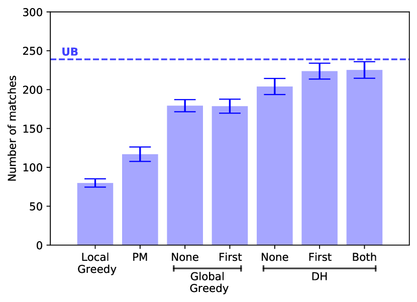
(a) Without Initial Backlog

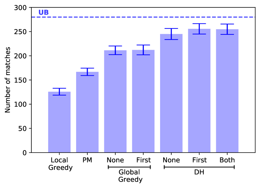
(b) With Initial Backlog

Figure 1: Matches by Benchmark

First, we observe that the performance of PM and Local Greedy are considerably better than their worst-case performance. Second, we observe that Global Greedy largely outperforms these benchmarks. Moreover, we find no significant differences in the number of matches obtained when considering simultaneous matches in the first period (i.e., comparing Global Greedy None vs. First). These results suggest that allowing simultaneous matches in the first period does not make a significant difference. Third, we find that DH and its variants outperform all the other benchmarks. Indeed, as we show in Proposition 6.1, this result holds more generally in the case of one-directional interactions and sequential matches.

Proposition 6.1

The DH algorithm has a performance guarantee at least as good as that of Algorithm 1 for the case with one-directional interactions and sequential matches.

Finally, we observe that if we only allow sequential matches (as in DH-None), the performance is relatively similar when both simultaneous and sequential matches are permitted. Indeed, when we assume no initial backlogs, DH-None achieves 90.56% of the matches generated by DH, while this number increases to 96.46% when considering initial backlogs. In addition, we observe that DH-First and DH-Both lead to almost identical results, suggesting that considering simultaneous matches in the second period while making first-period decisions plays no significant role. These results suggest that most matches are generated either sequentially and that considering simultaneous matches in the second period when choosing first-period assortments plays no significant role. Hence, these simulation results support the conjecture that the performance guarantees obtained for the case with simultaneous matches in the first period are similar to those for the general problem.

7 Conclusions

We theoretically study the two-sided assortment optimization problem that many dating platforms face when deciding the subset of profiles to show to each user in each period to maximize the expected number of matches. Motivated by the wide variaty of apps, we study different platform designs, varying (i) which side of the market can start an interaction, and (ii) whether the platform allows simultaneous matches. Using tools from submodular optimization, we provide performance guarantees for each variant of the problem. In addition, we show theoretically and through simulations that the improvement obtained from considering simultaneous matches is limited.

Managerial Implications.

Our results have several interesting managerial implications. First, our results show that natural approaches such as local greedy or non-adaptive policies are not suitable to our problem due to the two-sided nature of the problem. Hence, platforms should avoid these types of policies. Second, our results suggest that enabling simultaneous matches does not lead to a major improvement while significantly increasing the complexity of the problem. Third, our results show that limiting the analysis to policies with one period of lookahead is enough to capture most of the matches, also simplifying the analysis significantly. Therefore, platforms should focus on devising and improving algorithms that tackle the sequential variants of the problem with one period of lookahead. Finally, although we focus on dating platforms, we believe that many of these insights would translate to other two-sided assortment problems such as in freelancing, ride-sharing, among others.

Future Work.

There are many exciting directions for future research. First, our results suggests that the constant factor approximation derived for the case with both sequential and simultaneous matches can be improved. Second, we conjecture that the performance guarantee of $1/3$ also applies to the general case (multi-period with sequential and simultaneous matches in each period), so it would be worth exploring and confirming that this is true. Third, it would be interesting to extend our model to the case when like probabilities depend on the assortment shown, as this may be relevant in other markets where users can get at most one match (e.g., for a given date, hosts on Airbnb can match with at most one guest). Finally, it is worth studying performance guarantees when users log in with some known probability.

We would like to thank Victor Verdugo and Daniela Saban for the ideas discussed in earlier versions of this work. Also, we thank our industry partner for helpful discussions and for facilitating the data.

8 Appendix to Section 3

8.1 Dynamic programming formulation

Let $\mu_{\ell\ell^{\prime}}^{t}=1$ if a match between users $\ell$ and $\ell^{\prime}$ happens in period $t$, and $\mu_{\ell\ell^{\prime}}^{t}=0$ otherwise. As discussed in Section 3, $\mu_{\ell,\ell^{\prime}}^{t}=1$ if and only if one of the following three (disjoint) events takes place: (i) $\left\{\Phi_{\ell\ell^{\prime}}^{t}=1,\ell^{\prime}\in\mathcal{B}_{\ell}^{t}\right\}$, (ii) $\left\{\Phi_{\ell^{\prime}\ell}^{t}=1,\ell\in\mathcal{B}_{\ell^{\prime}}^{t}\right\}$, or (iii) $\left\{\Phi_{\ell\ell^{\prime}}^{t}=\Phi_{\ell^{\prime}\ell}^{t}=1\right\}$.

Given a set of potentials $\vec{\mathcal{P}}=\left\{\mathcal{P}_{\ell}\right\}_{\ell\in I\cup J}$ and a set of backlogs $\vec{\mathcal{B}}=\left\{\mathcal{B}_{\ell}\right\}_{\ell\in I\cup J}$, Problem 3.3 can be formulated as the following dynamic program:

$${\footnotesize\begin{split}V^{t}(\vec{\mathcal{P}},\vec{\mathcal{B}})&=\max_{\begin{subarray}{c}S_{\ell}\in\mathcal{P}_{\ell}\\ \left|S_{\ell}\right|\leq K_{\ell}\forall\ell\in I\cup J\end{subarray}}\left\{\mathbb{E}\left[\sum_{\ell\in I\cup J}\sum_{\ell^{\prime}\in S_{\ell}}\mu_{\ell\ell^{\prime}}^{t}\cdot\mathbbm{1}_{\left\{\ell^{\prime}\in\mathcal{B}_{\ell}\right\}}+\frac{1}{2}\cdot\mu_{\ell,\ell^{\prime}}^{t}\cdot\mathbbm{1}_{\left\{\ell\notin\mathcal{B}_{\ell}\right\}}+V^{t+1}\left(\vec{\mathcal{P}}\setminus\left(\vec{S}\cup\vec{R}\right),\vec{\mathcal{B}}\cup\vec{A}\setminus\vec{S}\right)\right]\right\}\\ V^{T+1}(\vec{\mathcal{P}},\vec{\mathcal{B}})&=0\end{split}}$$

where $\vec{A}=\left\{A_{\ell}\right\}_{\ell\in I\cup J}$ and $\vec{R}=\left\{R_{\ell}\right\}_{\ell\in I\cup J}$ are such that $A_{\ell}$ and $R_{\ell}$ represent the sets of users that liked and disliked $\ell$ in that period, i.e.,

$$\begin{split}A_{\ell}&=\left\{\ell^{\prime}\in\mathcal{P}_{\ell}:\ell\in S_{\ell}^{\prime},\Phi_{\ell^{\prime}\ell}=1\right\}\\ R_{\ell}&=\left\{\ell^{\prime}\in\mathcal{P}_{\ell}:\ell\in S_{\ell}^{\prime},\Phi_{\ell^{\prime}\ell}=0\right\}\\ \end{split}$$

Note that the first term in the summation ($\mu_{\ell\ell^{\prime}}^{t}\cdot\mathbbm{1}_{\left\{\ell^{\prime}\in\mathcal{B}_{\ell}\right\}}$) captures sequential matches, i.e., matches produced by cases (i) and (ii) mentioned above, while the second term ($\mu_{\ell,\ell^{\prime}}^{t}\mathbbm{1}_{\left\{\ell\notin\mathcal{B}_{\ell}\right\}}$) captures simultaneous matches generated produced by case (iii). The latter term is multiplied by 1/2 to avoid double-counting simultaneous matches.

8.2 Complexity

Proof 8.1

Proof of Proposition 3.2. To show that the problem is NP-hard, we show that we can reduce the set covering problem (SCP) to ours. An instance of SCP consists of a set of elements $\mathcal{U}$, a collection $\mathcal{C}=\left\{C_{1},\ldots,C_{m}\right\}$ such that $C_{i}\subseteq\mathcal{U}$ for all $i\in[m]$ and $\bigcup_{i\in[m]}C_{i}=\mathcal{U}$, and an integer $k$. The decision problem is whether there exists a cover of size at most $k<m$, i.e., a subset $\mathbf{C}\subseteq\mathcal{C}$ such that $\left|\mathbf{C}\right|\leq k\text{ and }\mathcal{U}\subseteq\bigcup_{C\in\mathbf{C}}C$.

Given an instance of $SCP$, we construct the following instance of our problem. We consider two sides of the market, $I=\left\{1,\ldots,m\right\}$ and $J=\mathcal{U}\cup\bigcup_{i=1}^{m}D_{i}$, where $D_{i}$ is a set of unique duplicates of the elements of $C_{i}$. Each user $i\in I$ has an initial set of potentials $\mathcal{P}_{i}=C_{i}\cup D_{i}$, while each user $j\in J$ is such that $\mathcal{P}_{j}=I$. For each $i\in I$, we assume that

$$\phi_{ij}=\begin{cases}1&\text{if }j\in C_{i}\\ \frac{1}{m\cdot\bar{c}\cdot\left|C_{i}\right|}&\text{if }j\in D_{i}\\ 0&\text{otherwise}\end{cases}$$

where $\bar{c}=\max_{i\in[m]}\left|C_{i}\right|$. In contrast, we assume that $\phi_{j,i}=1$ for all $j\in J$ and $i\in\mathcal{P}_{j}$. Finally, we assume that the assortment size of each user $i\in I$ is $K_{i}=\left|C_{i}\right|$, while the assortment size for each user $j\in J$ is $K_{j}=1$, and we assume no initial backlogs, i.e., $\mathcal{B}_{\ell}=\emptyset$ for all $\ell\in I\cup J$.

We show that a set cover exists for the instance $\left(\mathcal{U},\mathcal{C},k\right)$ if the number of matches obtained from the instance of the assortment problem described above is at least $\left|\mathcal{U}\right|+\frac{(m-k)}{m\cdot\bar{c}}$.

$\Rightarrow$ Suppose that there exists a set cover of size $k$, $\mathbf{C}=\left\{C_{i_{1}},\ldots,C_{i_{k}}\right\}$. for convenience, let $I^{\prime}=\left\{i_{1},\ldots,i_{k}\right\}$ the set of indices that provide the cover $\mathbf{C}$. Then, we construct a solution for the assortment problem that achieves an expected number of matches of at least $\left|\mathcal{U}\right|+\frac{(m-k)}{m\cdot\bar{c}}$ as follows. Each user $i\in I^{\prime}$ observes an assortment $S_{i}^{1}=C_{i}$ in the first period, and an empty assortment in the next period. Each user $i\in I\setminus I^{\prime}$ observes an assortment $S_{i}^{1}=D_{i}$ in the first period, and an empty assortment in the second period. Finally, each user $j\in J$ observes an empty assortment in the first period and, in the second period, an assortment containing one of the users that saw them in the first period (if any), i.e., $S_{j}^{2}\in\left\{i\in I:j\in S_{i}\right\}$. If multiple users in $I$ see the same $j\in J$, then we assume that $j$ sees each of them back with probability $1/\left|i\in I:j\in S_{i}^{1}\right|$.

First, note that the cardinality constraints are satisfied, since $S_{i}^{1}$ is either $C_{i}$ or $D_{i}$, both of which have cardinality $\left|C_{i}\right|=K_{i}$, and users $j\in J$ see at most one profile in the second period. Moreover, note that all assortments $S_{\ell}^{t}\subseteq\mathcal{P}_{\ell}$ for all $\ell\in I\cup J$, and thus they are feasible. Second, since $\mathbf{C}$ is a cover, we know that $\mathcal{U}\subseteq\bigcup_{C\in\mathbf{C}}C$, and thus each element in $\mathcal{U}$ is seen by at least one user $i\in I$. Since $\phi_{i,j}=1$ and $\phi_{j,i}=1$ for $i\in I$ and $j\in C_{i}$, we know that each $j\in\mathcal{U}$ will be liked by someone in $I^{\prime}$, and that they will like back at least one of the users that saw them. Hence, all users in $\mathcal{U}$ will get one match with users in the set $I^{\prime}$. Finally, note that all users $i\in I\setminus I^{\prime}$ observe assortments $S_{i}^{1}=D_{i}$, and like each of these profiles with probability $\frac{1}{m\cdot\bar{c}\cdot\left|C_{i}\right|}$. Then, these users are liked back with probability 1, since $\phi_{ji}=1$ for all $j\in J,\;i\in\mathcal{P}_{j}$ and the fact that these duplicates are seen by at most one user. Hence, the users $i\in I\setminus I^{\prime}$ obtain a expected number of matches equal to

$$\sum_{j\in S_{i}^{t}}\frac{1}{m\cdot\bar{c}\cdot\left|C_{i}\right|}\cdot 1=\left|D_{i}\right|\cdot\frac{1}{m\cdot\bar{c}\cdot\left|C_{i}\right|}=\frac{1}{m\cdot\bar{c}},$$

where the first equality follows from $S_{i}^{t}=D_{i}$ and the second follows from $D_{i}$ been a duplicate of the set $C_{i}$, and thus $\left|D_{i}\right|=\left|C_{i}\right|$. Hence, the expected number of matches generated by users in $I\setminus I^{\prime}$ is $(m-k)\cdot\frac{1}{m\cdot\bar{c}}$, and thus the total expected number of matches is $\left|\mathcal{U}\right|+\frac{(m-k)}{m\cdot\bar{c}}$.

$\Leftarrow$ Suppose that there exists a solution to the assortment problem $\bar{S}=\left(\left\{S_{i}\right\}_{i\in I},\left\{S_{j}\right\}_{j\in J}\right)$ that produces an expected number of matches of at least $\left|\mathcal{U}\right|+\frac{(m-k)}{m\cdot\bar{c}}$. First, note that the only way to obtain at least $\left|\mathcal{U}\right|$ matches is by covering all the elements of $\mathcal{U}$, since every user in $J$ sees at most one profile (and thus belongs to at most one match), and every user in $J\setminus\mathcal{U}$ generates a match with probability at most $\frac{1}{m\cdot\bar{c}\cdot\underline{c}}\ll 1$, where $\underline{c}=\min_{i\in[m]}\left\{C_{i}\right\}$. Hence, we know that $\left\{S_{i}^{1}\right\}_{i\in I}$ is a cover of $\mathcal{U}$. It remains to show that we can find a $k$ elements of $\left\{S_{i}^{1}\right\}_{i\in I}$ that are enough to cover $\mathcal{U}$. To see this, suppose that this is not the case, i.e., we need at least $k+1$ elements in $\left\{S_{i}^{1}\right\}_{i\in I}$ to cover $\mathcal{U}$. Then, there are less than $m-k$ users in $I$ who see assortments containing exclusively duplicated elements, i.e., $\left|\left\{i\in I:S_{i}^{1}\subseteq D_{i}\right\}\right|<m-k$. Then, the expected number of matches generated by these users is strictly less than $(m-k)\cdot\frac{1}{m\cdot\bar{c}}$. Finally, since every element in $\mathcal{U}$ generates at most one match in expectation, we conclude that the total number of matches is strictly less than $\left|\mathcal{U}\right|+(m-k)\cdot\frac{1}{m\cdot\bar{c}}$, which contradicts our hypothesis.

8.3 Offline Optimum versus Online Optimum

Consider the following instance taken from Chen et al. (2009): There are $n$ users in $I$ and $n$ users in $J$. The probabilities are all $\phi_{i,j}=(2\log n)/n$ and $\phi_{j,i}=1$ for all $j\in J,\ i\in I$. Therefore $\beta_{e}=2\log n/n$ for each edge. Consider $1$ stage and $K_{\ell}=1$. According to Erdős and Rényi (1964, 1968), with constant probability there exists a perfect matching which means that the value of the omniscient optimum is $c\cdot n$ for some constant $c>0$. On the other hand, a one-directional policy will show $S_{i_{k}}=\{j_{k}\}$ which will produce a matching of expected size $2\log n$ and this is optimal. Therefore, the gap is $O(\frac{\log n}{n})$.

8.4 Natural Approaches

Proof 8.2

Proof of Proposition 3.5. Suppose that there are $n$ users on each side of the market, i.e., $I=\left\{i_{1},\ldots,i_{n}\right\}$ and $J=\left\{j_{1},\ldots,j_{n}\right\}$. In addition, suppose that $\mathcal{P}_{i}=J$ for every $i\in I$, $\mathcal{P}_{j}=I$ for every $j\in J$. Let us set the probabilities: $\beta^{1}_{ij}=1$ for $j=j_{1}$ and for all $i\in I$, $\beta^{1}_{ij}=1-\varepsilon$ for all $i\in I$ and $j\neq j_{1}$, while $\beta^{2}_{ij}=0$ for all $i\in I\cup J,\,j\in\mathcal{P}_{i}$. In this setting, the greedy policy will chose $S^{1}_{i}=\left\{j_{1}\right\}$ for every user $i$, and therefore only one match will take place in expectation. In contrast, an optimal solution is to assign $S^{1}_{i_{k}}=\left\{j_{k}\right\}$, which leads to $1+(n-1)(1-\varepsilon)$ matches in expectation. Then, the performance of the greedy policy is given by $1/(1+(n-1)(1-\varepsilon))\to 0$, as $n\rightarrow\infty$ for $\varepsilon$ sufficiently small.

Proof 8.3

Proof of Proposition 3.6. Suppose that $\left|I\right|=2n$, $\left|J\right|=2$, that $\mathcal{P}^{1}_{i}=J$ for every $i\in I$, $\mathcal{P}^{1}_{j}=I$ for every $j\in J$, and that $\phi^{t}_{ij}=p$ while $\phi^{t}_{ji}=q$ for all $i\in I,\;j\in J$, and $t\in\{1,2\}$. Then, it is easy to see that the sequential perfect match policy leads to $4pq$ matches in expectation. On the other hand, consider the policy where: (i) In $t=1$, $\left\{i_{1},\ldots,i_{n}\right\}$ see $j_{1}$, $\left\{i_{n+1},\ldots,i_{2n}\right\}$ see $j_{2}$, $j_{1}$ sees $i_{2n}$ and $j_{2}$ sees $i_{1}$, and (ii) in $t=2$, $\left\{i_{1},\ldots,i_{n}\right\}$ see $j_{2}$, $\left\{i_{n+1},\ldots,i_{2n}\right\}$ see $j_{1}$, $j_{1}$ sees any profile that liked her in $t=1$, and same for $j=2$. Given this policy, the matches $(i_{2n},j_{1})$ and $(i_{1},j_{2})$ happen with probability $pq$ each. On the other hand, $j_{1}$ matches with someone in $\left\{i_{1},\ldots,i_{n}\right\}$ with probability $(1-(1-p)^{n})q$, and the same for $j_{2}$ matching with someone in $\left\{i_{n+1},\ldots,i_{2n}\right\}$. Then, the total expected number of matches is $2pq+2q(1-(1-p)^{n})$, which is optimal for this instance. Then, the sequential perfect match policy achieves a performance of $4pq/(2q(p+1-(1-p)^{n}))\to 2/(1+n)$ when $p\rightarrow 0$, and since $2/(1+n)\to 0$ when $n\to\infty$, we conclude the proof.

Proof 8.4

Proof of Proposition 3.7. Consider the following instance: $I=\{1,\ldots,n\}$, $J=\{j\}$, $K_{i}=K_{j}=1$, $\phi_{i,j}=1/n$ and $\phi_{ji}=1$ for all $i\in I$. If we only allow sequential shows, then any deterministic non-adaptive policy would have an expected value of at most $1/n$, since we are choosing pairs $i,j$ in advance without looking at the backlogs. However, the optimal adaptive policy consists of: showing $j$ to every $i\in I$ in the first stage, and if there is at least one agent $i\in I$ that likes $j$ then show this agent to $j$ in the second stage. The optimal value in this case is the probability that $j$ is liked by at least one person, i.e., $1-(1-1/n)^{n}\to 1-1/e$. If we allow simultaneous shows, the ratio is still arbitrarily close to zero.

9 Appendix to Section 4

9.1 Missing Proofs in Section 4.1

Proof 9.1

Proof of Lemma 4.4. The set of potentials $\mathcal{P}_{i}^{1}$ for all $i\in I$ partitions the set of edges $\mathcal{E}=\vec{E}_{I}$ and the budget of each part corresponds to $K_{i}$.

Proof 9.2

Proof of Lemma 4.5. Similar to Lemma 4.4 but the partition is restricted to the corresponding elements in the backlog.

Proof 9.3

Proof of Lemma 4.7. Let us prove then that $\mathcal{M}(\mathbf{x})$ is a non-negative monotone submodular function. Recall that $f$ is a non-negative, monotone submodular function due to Corollary 4.6. Since $f$ is non-negative, then $\mathcal{M}$ is also non-negative. For $\mathbf{x}\in\{0,1\}^{\mathcal{E}}$, denote by $\text{supp}(\mathbf{x})=\{a\in\mathcal{E}:\ x_{a}l=1\}$ the support of $\mathbf{x}$. Then, we can write $\mathcal{M}$ as follows

$$\mathcal{M}(\mathbf{x})=\sum_{\mathbf{B}\subseteq\text{supp}(\mathbf{x})}f(\mathbf{B})\prod_{a\in\mathbf{B}}\phi_{a}^{1}\prod_{a\in\text{supp}(\mathbf{x})\setminus B}(1-\phi_{a}^{1})$$

On the other hand, for any $e\notin\text{supp}(x)$ we have

$$\mathcal{M}(\mathbf{x}+\mathbbm{1}_{\left\{e\right\}}) =\phi_{e}^{1}\cdot\sum_{B\subseteq\text{supp}(\mathbf{x})}f(B+e)\prod_{a\in\mathbf{B}}\phi_{a}^{1}\prod_{a\in\text{supp}(\mathbf{x})\setminus B}(1-\phi_{a}^{1})$$

$$+(1-\phi_{e}^{1})\cdot\sum_{B\subseteq\text{supp}(\mathbf{x})}f(B)\prod_{a\in\mathbf{B}}\phi_{a}^{1}\prod_{a\in\text{supp}(\mathbf{x})\setminus B}(1-\phi_{a}^{1})$$

Therefore,

$$\mathcal{M}(\mathbf{x}+\mathbbm{1}_{\left\{e\right\}})-\mathcal{M}(\mathbf{x})=\phi_{e}^{1}\sum_{B\subseteq\text{supp}(\mathbf{x})}[f(B+e)-f(B)]\prod_{a\in\mathbf{B}}\phi_{a}^{1}\prod_{a\in\text{supp}(\mathbf{x})\setminus B}(1-\phi_{a}^{1})$$

Since $f$ is monotone, then $f(B+e)-f(B)\geq 0$ for all $B\subseteq\text{supp}(\mathbf{x})$ and $e\notin\text{supp}(\mathbf{x})$, which implies $\mathcal{M}(\mathbf{x}+\mathbbm{1}_{\left\{e\right\}})-\mathcal{M}(\mathbf{x})\geq 0$.

Now, let us prove that $\mathcal{M}$ is submodular. Consider any $\mathbf{x}\in\{0,1\}^{\mathcal{E}}$ and $e,e^{\prime}\notin\text{supp}(\mathbf{x})$. Our goal is to show that $\mathcal{M}(\mathbf{x}+\mathbbm{1}_{\left\{e\right\}})-\mathcal{M}(\mathbf{x})\geq\mathcal{M}(\mathbf{x}+\mathbbm{1}_{\left\{e\right\}}+\mathbbm{1}_{\left\{e^{\prime}\right\}})-\mathcal{M}(\mathbf{x}+\mathbbm{1}_{\left\{e^{\prime}\right\}})$. Note that we have the following expression for $\mathcal{M}(\mathbf{x}+\mathbbm{1}_{\left\{e\right\}}+\mathbbm{1}_{\left\{e^{\prime}\right\}})$

$$\mathcal{M}(\mathbf{x}+\mathbbm{1}_{\left\{e\right\}}+\mathbbm{1}_{\left\{e^{\prime}\right\}}) =\phi_{e}^{1}\phi_{e^{\prime}}^{1}\cdot\sum_{B\subseteq\text{supp}(\mathbf{x})}f(B+e+e^{\prime})\prod_{a\in\mathbf{B}}\phi_{a}^{1}\prod_{a\in\text{supp}(\mathbf{x})\setminus B}(1-\phi_{a}^{1})$$

$$+\phi_{e^{\prime}}^{1}(1-\phi_{e}^{1})\cdot\sum_{B\subseteq\text{supp}(\mathbf{x})}f(B+e^{\prime})\prod_{a\in\mathbf{B}}\phi_{a}^{1}\prod_{a\in\text{supp}(\mathbf{x})\setminus B}(1-\phi_{a}^{1})$$

$$+\phi_{e}(1-\phi_{e^{\prime}}^{1})\cdot\sum_{B\subseteq\text{supp}(\mathbf{x})}f(B+e)\prod_{a\in\mathbf{B}}\phi_{a}^{1}\prod_{a\in\text{supp}(\mathbf{x})\setminus B}(1-\phi_{a}^{1})$$

$$+(1-\phi_{e^{\prime}}^{1})(1-\phi_{e}^{1})\cdot\sum_{B\subseteq\text{supp}(\mathbf{x})}f(B)\prod_{a\in\mathbf{B}}\phi_{a}^{1}\prod_{a\in\text{supp}(\mathbf{x})\setminus B}(1-\phi_{a}^{1})$$

Analogously, we can compute $\mathcal{M}(\mathbf{x}+\mathbbm{1}_{\left\{e\right\}})$ and $\mathcal{M}(\mathbf{x}+\mathbbm{1}_{\left\{e^{\prime}\right\}})$. By deleting common terms, we can obtain the following

$$\mathcal{M}(\mathbf{x}+\mathbbm{1}_{\left\{e\right\}})-\mathcal{M}(\mathbf{x})-\mathcal{M}(\mathbf{x}+\mathbbm{1}_{\left\{e\right\}}+\mathbbm{1}_{\left\{e^{\prime}\right\}})+\mathcal{M}(\mathbf{x}+\mathbbm{1}_{\left\{e^{\prime}\right\}})$$

$$=\phi_{e}^{1}\phi_{e^{\prime}}^{1}\cdot\sum_{B\subseteq\text{supp}(\mathbf{x})}[f(B+e)-f(B)-f(B+e+e^{\prime})+f(B+e^{\prime})]\prod_{a\in\mathbf{B}}\phi_{a}^{1}\prod_{a\in\text{supp}(\mathbf{x})\setminus B}(1-\phi_{a}^{1}),$$

from which submodularity follows due to submodularity of $f$.

Proof 9.4

Proof of Lemma 4.9. Consider a feasible solution $\mathbf{x}^{1}\in\{0,1\}^{\mathcal{E}}$ for the optimization problem (6), that is, $\sum_{j\in J}x^{1}_{(i,j)}\leq K$ for every $i\in I$. Let $\mathbf{z}=\phi^{1}\mathbf{x}^{1}$. Observe that

$$\sum_{j\in J:\phi^{1}_{ij}>0}z_{ij}/\phi^{1}_{ij}=\sum_{j\in J:\phi^{1}_{ij}>0}x^{1}_{(i,j)}\leq K_{i}$$

for every $i\in I$, and $z_{a}=x^{1}_{a}\phi^{1}_{a}\leq\phi^{1}_{a}$ for every $a\in\mathcal{E}$. Therefore $\mathbf{z}$ is a feasible solution for the problem (8a)-(8c). Since the objective value of $\mathbf{x}^{1}$ in (6) is equal to the objective of $\mathbf{z}$ in (8a)-(8c), we conclude the lemma.

Proof 9.5

Proof of Theorem 4.8. Thanks to condition (1) of the randomized rounding algorithm, for each $i\in I$ we have $\sum_{j\in J}\hat{x}_{ij}\leq\left\lceil\sum_{j\in J}x_{ij}\right\rceil=\lceil\sum_{j\in J:\phi_{ij}>0}\tilde{z}_{ij}/\phi_{ij}^{1}\rceil\leq K_{i},$ where the last inequality holds since $K_{i}$ is integral and $\tilde{\mathbf{z}}$ satisfies constraint (8b). Therefore, our algorithm gives a feasible solution for Problem (6). We now analyze the approximation guarantee.

$$\mathbb{E}_{\mathbf{\mathcal{B}}\sim\mathbf{\phi}^{1}\hat{\mathbf{x}}}\left[f(\mathbf{\mathcal{B}})\right] =\sum_{\mathbf{B}\subseteq\mathcal{E}}f(\mathbf{B})\cdot\text{I\kern-1.49994ptP}_{\hat{\mathbf{x}}}\left(\mathbf{\mathcal{B}}=B\right)$$

$$=\sum_{\mathbf{B}\subseteq\mathcal{E}}f(\mathbf{B})\cdot\mathbb{E}_{\hat{\mathbf{x}}}\left[\prod_{a\in\mathbf{B}}\phi^{1}_{a}\hat{x}_{a}\prod_{a\notin B}(1-\phi^{1}_{a}\hat{x}_{a})\right]$$

$$=\sum_{\mathbf{B}\subseteq\mathcal{E}}f(\mathbf{B})\cdot\prod_{a\in\mathbf{B}}\phi^{1}_{a}\mathbb{E}_{\hat{\mathbf{x}}}[\hat{x}_{a}]\prod_{a\notin B}(1-\phi^{1}_{a}\mathbb{E}_{\hat{\mathbf{x}}}[\hat{x}_{a}])$$

$$=\sum_{\mathbf{B}\subseteq\mathcal{E}}f(\mathbf{B})\cdot\prod_{a\in\mathbf{B}}\phi^{1}_{a}\cdot\frac{\tilde{z}_{a}}{\phi^{1}_{a}}\prod_{a\notin B}(1-\phi^{1}_{a}\cdot\frac{\tilde{z}_{a}}{\phi^{1}_{a}})=\mathcal{M}(\tilde{z}),$$

where the second equality comes from the fact that $\hat{\mathbf{x}}_{i}$ is independent from $\hat{\mathbf{x}}_{i^{\prime}}$ for every $i,i^{\prime}\in I$ with $i\neq i^{\prime}$ and the third equality comes from condition 2 of the randomized rounding procedure. Finally, Lemma 4.9 states that $\text{OPT}^{\prime}\geq\text{OPT}$, where $\text{OPT}^{\prime}$ is the optimal value of Problem  (8a)-(8c), so we conclude the proof by using Corollary (4.10).

9.2 Missing Proofs in Section 4.2

Proof 9.6

Proof of Lemma 4.11. Our ground set of elements is $\mathcal{E}=\vec{E}_{I}\cup\vec{E}_{J}$. The first partition consists of the following parts: $\mathcal{E}_{\ell}=\{e:e=(\ell,\ell^{\prime})\ \text{for every}\ \ell^{\prime}\in\mathcal{P}_{\ell}\}$ for all $\ell\in I\cup J$. It is easy to check that $\mathcal{E}=\cup_{\ell\in I\cup J}\mathcal{E}_{\ell}$ and $\mathcal{E}_{\ell}\cap\mathcal{E}_{\ell^{\prime}}=\emptyset$ for every $\ell,\ell^{\prime}$ such that $\ell\neq\ell^{\prime}$. Finally, the budget for each part $\mathcal{E}_{\ell}$ is $K_{\ell}$. Now, let us construct the second partition matroid. For every pair $i\in I$ and $j\in J$, we define a part $\mathcal{E}_{i,j}$ as the set $\{(i,j),(j,i)\}$. Indeed this forms a partition of $\mathcal{E}$. Finally, the budget for each part $\mathcal{E}_{i,j}$ is 1.

Proof 9.7

Proof of Theorem 4.12. Consider the formulation (6) of Problem 3.3. Since $\mathbf{x}^{1}$ is a 0-1 vector and $\mathcal{M}(\cdot)$ is monotone submodular over elements in $\mathcal{E}$, we know that a vanilla greedy algorithm achieves a $1/(1+r)$-approximation for the problem of maximizing a monotone submodular function over the intersection of $r$ matroids Fisher et al. (1978) and local-search guarantees a factor of $1/(r+\epsilon)$ for any fixed $\epsilon>0$ (Lee et al. 2009). By Lemma 4.2 we know that $r=2$, and thus the guarantee is $1/3$ for greedy and $1/(2+\epsilon)$ for local-search.

9.3 Missing Proofs in Section 4.3

Before proving the next result, let us consider the following definition:

Definition 9.8 (Laminar Matroid)

A family $\mathcal{X}\subseteq 2^{\mathcal{E}}$ over a ground set of elements $\mathcal{E}$ is called laminar if for any $X,Y\in\mathcal{X}$ we either have $X\cap Y=\emptyset$, $X\subseteq Y$ or $X\subseteq Y$. Assume that for each element $u\in\mathcal{E}$ there exists some $A\in\mathcal{X}$ such that $A\ni u$. For each $A\in\mathcal{X}$ let $c(A)$ a positive integer associated with it. A laminar matroid $\mathcal{I}$ is defined as $\mathcal{I}=\{A\subseteq\mathcal{E}:\ |A\cap X|\leq c(X)\ \forall X\in\mathcal{X}\}$.

Proof 9.9

Proof of Lemma 4.13. First, let us defined our laminar family $\mathcal{X}$. For every pair $i\in I,j\in J$ consider $X_{i,j}=\{(i,j),\{i,j\}\}$, also for every $i\in I$ consider $Y_{i}=\{(i,\ell):\ell\in\mathcal{P}_{i}\}\cup\{\{i,\ell\}:\ell\in\mathcal{P}_{i}\}$. Indeed, this is a laminar family, two sets of type $X$ do not intersect and two sets of type $Y$ also do not intersect. Sets of type $X$ and $Y$ intersect only if they correspond to the same $i\in I$ in which case $X_{i,j}\subseteq Y_{i}$. Finally, for every $X_{i,j}$ we have $c(X_{i,j})=1$ and for each $Y_{i}$ we have $c(Y_{i})=K_{i}$. Therefore, for this laminar family $\mathcal{S}$ and values $c(\cdot)$ we have that $\mathcal{I}=\{A\subseteq\mathcal{E}:\ |A\cap X|\leq c(X)\ \forall X\in\mathcal{S}\}$ coincides with feasible region $Q^{1}$. The partition matroid is defined by the following parts: for each $j\in J$ consider $\mathcal{E}_{j}=\{\{i,j\}:\ i\in\mathcal{P}_{j}\}$ and $\mathcal{E}_{0}=\mathcal{E}\setminus\bigcup_{j\in J}\mathcal{E}_{j}$. The budget for each part $\mathcal{E}_{j}$ is $K_{j}$ and for $\mathcal{E}_{0}$ is $|\mathcal{E}_{0}|$.

Proof 9.10

Proof of Theorem 4.14. Similar to the proof of Theorem 4.12.

9.4 Missing Proofs in Section 4.4

Proof 9.11

Proof of Lemma 4.15. As in Lemma 4.11, the first partition consists of the following parts: $\mathcal{E}_{i}=\{\{(i,j),\{i,j\}\}:\ \text{for every}\ j\in\mathcal{P}_{i}\}$ for all $i\in I$ and $\mathcal{E}_{0}=\mathcal{E}\setminus\cup_{i\in I}\mathcal{E}_{i}$. It is easy to check that $\mathcal{E}=\mathcal{E}_{0}\cup\bigcup_{i\in I}\mathcal{E}_{\ell}$ and $\mathcal{E}_{\ell}\cap\mathcal{E}_{\ell^{\prime}}=\emptyset$ for every $\ell,\ell^{\prime}\in I\cup\{0\}$ such that $\ell\neq\ell^{\prime}$. Finally, the budget for each part $\mathcal{E}_{i}$ is $K_{i}$ for every $i\in I$ and $|\mathcal{E}_{0}|$ for $\mathcal{E}_{0}$. Analogously, we can construct the second partition matroid by considering parts: $\mathcal{E}_{i}j=\{\{(j,i),\{i,j\}\}:\ \text{for every}\ i\in\mathcal{P}_{j}\}$ for all $j\in J$ and $\mathcal{E}_{0}=\mathcal{E}\setminus\cup_{j\in J}\mathcal{E}_{j}$. The final partition is composed by the following parts: For every pair $i\in I$ and $j\in J$, we define a part $\mathcal{E}_{i,j}$ as the set $\{(i,j),(j,i),\{i,j\}\}$. Indeed this forms a partition of $\mathcal{E}$. Finally, the budget for each part $\mathcal{E}_{i,j}$ is 1.

Proof 9.12

Proof of Theorem 4.16. Similar to the proof of Theorem 4.12.

10 Appendix to Section 5

10.1 Simultaneous Matches in both Periods and One-Directional Interactions

Proof 10.1

Proof of Proposition 5.1. Given a realized backlog $\mathbf{B}=\left\{B_{l}\right\}_{\ell\in I\cup J}$ and a set of potentials $\mathcal{P}$, define a bipartite graph with two sides $U,V$ with $U=I\cup J$ and $V=B\cup\left\{(i,j)\in I\times J\;:\;j\in\mathcal{P}_{i},i\in\mathcal{P}_{j}\right\}$, i.e., $U$ contains the set of users and $V$ the set of arcs that could be displayed in the second period. Let $E\subseteq U\times V$ be the set of edges. Then, a pair $\left(\ell,(\ell^{\prime},\ell^{\prime\prime})\right)\in U\times V$ belongs to $E$ if and only if

$$(\ell^{\prime},\ell^{\prime\prime})\in B_{\ell}\quad\text{ or }\quad\left[(\ell^{\prime},\ell^{\prime\prime})\notin B_{\ell},\ell\in\left\{\ell^{\prime},\ell^{\prime\prime}\right\}\right].$$

In words, an edge between $\ell\in U$ and $(\ell^{\prime},\ell^{\prime\prime})\in V$ exists if and only if the edge $(\ell^{\prime},\ell^{\prime\prime})$ is either in the backlog of $\ell$ or both users $\ell$ and $\ell^{\prime}$ can see each other simultaneously. Now, for any pair of nodes $(u,v)\in E$ such that $v\in\mathbf{B}$, we define a variable $y_{u,v}$ that is equal to 1 if $v=(u,u^{\prime})\in B_{u}$ and $u$ sees $u^{\prime}$, and zero otherwise. Similarly, for any pair $(u,v)\in E$ such that $v=(u,u^{\prime})\in V\setminus\mathbf{B}$, we define a variable $x_{u,v}$ that is equal to 1 if $u$ sees $u^{\prime}$, and zero otherwise. Note that here we do a slight abuse of notation and assume that if $x_{i,(i,j)}=1$, then $i\in I$ sees profile $j\in P_{i}\setminus B_{i}$ and, similarly, if $x_{j,(i,j)}=1$, then $j\in J$ sees $i\in P_{j}\setminus B_{j}$. For convenience, we will use in these cases that $i\in(i,j)$ and $j\in(i,j)$. Finally, for any pair $(u,v)\in E$ such that $u\in I$ and $v\in V\setminus\mathbf{B}$, let $w_{u,v}=1$ if both users involved in $v$ see each other simultaneously, i.e., if $v=(i,j)\in V\setminus\mathbf{B}$, then $x_{i,(i,j)}=x_{j,(i,j)}=1$.

Using these variables, we can formulate the second period problem as follows:

$$f(\mathbf{B}):=\max\quad \quad\sum_{u\in U}\sum_{v\in\mathbf{B}}y_{u,v}\cdot\phi_{v}^{2}+\sum_{i\in I}\sum_{\delta(i)\cap V\setminus\mathbf{B}}w_{i,v}\cdot\beta_{v}^{2}$$ (19a)

$$st.\quad \quad\sum_{v\in\delta(u)\cap\mathbf{B}}y_{u,v}+\sum_{v\in\delta(u)\cap V\setminus\mathbf{B}}x_{u,v}\leq K_{u},\quad\forall u\in U$$ (19b)

$$\quad w_{i,(i,j)}-x_{u,(i,j)}\leq 0,\quad\forall(i,j)\in V\setminus\mathbf{B},i\in I,u\in(i,j)$$ (19c)

$$\quad w_{i,(i,j)}-x_{u,(i,j)}\leq 0,\quad\forall(i,j)\in V\setminus\mathbf{B},i\in I,u\in(i,j)$$ (19d)

$$\quad x_{u,v}\in\left\{0,1\right\},\quad v\in V\setminus\mathbf{B},u\in v$$ (19e)

$$\quad y_{u,v}\in\left\{0,1\right\},\quad\forall u\in U,v\in\delta(u)\cap\mathbf{B}$$ (19f)

$$\quad w_{i,v}\in\left\{0,1\right\},\quad\forall v\in V\setminus\mathbf{B},i\in v$$ (19g)

where $\beta_{v}^{2}=\phi_{v}^{2}\cdot\phi_{\overline{v}}^{2}$ is the match probability between the users in the pair $v$ and $\delta(u)$ is the set of edges incident to node $u\in U$. Let $Q^{2}$ be the set of constraints in (19b), (19c) and (19d). Note that each variable appears at most twice in $Q^{2}$, and that every time they appear they are multiplied by either 1 or -1. Thus, to show that the matrix of constraints if totally unimodular, it remains to show that the constraints in $Q^{2}$ can be separated in two subsets such that (i) if a variable appears twice with different signs, then the constraints belong to the same subset, and (ii) if a variable appears twice with the same sign, then the constraints belong to different subsets. Let $Q^{2}_{I}$ and $Q^{2}_{J}$ be the subsets of constraints of $Q^{2}$ involving $u\in I$ and $u\in J$, respectively. Then, observe that

• each $w_{i,(i,j)}$ appears in two constraints with the same sign ($w_{i,(i,j)}-x_{i,(i,j)}\leq 0$ and $w_{i,(i,j)}-x_{j,(i,j)}\leq 0$), but these constraints belongs to $Q_{I}^{2}$ and $Q_{J}^{2}$, respectively.

• each $x_{i,(i,j)}$ appears in two constraints with different signs ($\sum_{v\in\delta(i)\cap B_{i}}y_{i,v}+\sum_{v\in\delta(i)\cap V\setminus B_{i}}x_{i,v}\leq K_{i}$ and $w_{i,(i,j)}-x_{i,(i,j)}\leq 0$), but these constraints belong both to the same subset $Q_{I}^{2}$. Similarly, $x_{j,(i,j)}$ appears in two constraints with different signs, but both constraints belong to $Q_{J}^{2}$.

Hence, using Hoffman’s sufficient condition, we conclude that the constraints in $Q^{2}$ can be written as the product of a totally unimodular matrix and our vector of decisions variables. Finally, since the right-hand sides of the constraints are integral, we conclude that the feasible region of the problem is an integral polyhedron, and thus we can solve its linear relaxation.

Proof 10.2

Proof of Proposition 5.2. Let $\mathcal{Y}(\mathbf{B})$ and $\mathcal{Z}(\mathbf{B})$ be the sets of backlog and non-backlog pairs shown in the optimal solution of the second period problem. Consider the following example. Let $I=\left\{i_{1},i_{2}\right\},\;J=\left\{j_{1},j_{2}\right\}$, and the following probabilities:

$$\phi_{i_{1},j_{1}}=1,\phi_{j_{1},i_{1}}=\epsilon,\phi_{i_{2},j_{2}}=\epsilon,\phi_{j_{2},i_{2}}=1,\beta_{i_{1},j_{2}}=1/2,\beta_{i_{2},j_{1}}=1/2.$$

If $\mathbf{B}=\emptyset$, then $\mathcal{Z}(\mathbf{B})=\left\{(i_{1},j_{2}),(i_{2},j_{1})\right\}$. If we add $b=(i_{2},j_{2})$ to the backlog, then $\mathcal{Z}(\mathbf{B}\cup\left\{(i_{2},j_{2})\right\})=\left\{(i_{2},j_{1})\right\}$ and $\mathcal{Y}(\mathbf{B}\cup\left\{(i_{2},j_{2})\right\})=\left\{(j_{2},i_{2})\right\}$. Hence,

$$f(\mathbf{B}\cup\left\{(i_{2},j_{2})\right\})-f(\mathbf{B})=1+1/2-(1/2+1/2)=1/2.$$

On the other hand, if $\mathbf{B}^{\prime}=\left\{(j_{1},i_{1})\right\}$, $\mathcal{Z}(\mathbf{B}^{\prime})=\left\{(i_{2},j_{1})\right\}$ and $\mathcal{Y}(\mathbf{B}^{\prime})=\left\{(i_{1},j_{1})\right\}$. If we add $b=(i_{2},j_{2})$ to $\mathbf{B}^{\prime}$, then $\mathcal{Z}(\mathbf{B}^{\prime}\cup\left\{(i_{2},j_{2})\right\})=\left\{(i_{2},j_{1})\right\}$ and $\mathcal{Y}(\mathbf{B}^{\prime}\cup\left\{(i_{2},j_{2})\right\})=\left\{(i_{1},j_{1}),(j_{2},i_{2})\right\}$. Then,

$$f(\mathbf{B}^{\prime}\cup\left\{(i_{2},j_{2})\right\})-f(\mathbf{B}^{\prime})=1+1+1/2-(1+1/2)=1.$$

Hence, we have that

$$\mathbf{B}\subset\mathbf{B}^{\prime}\quad\text{ and }\quad f(\mathbf{B}\cup\left\{(i_{2},j_{2})\right\})-f(\mathbf{B})<f(\mathbf{B}^{\prime}\cup\left\{(i_{2},j_{2})\right\})-f(\mathbf{B}^{\prime}),$$

so we conclude that $f(\mathbf{B})$ is not submodular.

10.1.1 Proof of Theorem 5.3.

Recall function $f$ defined in (3) as

$$f(\mathbf{B})=\max_{\mathbf{x}^{2}\in P^{2}_{\mathbf{B}}}\Bigg{\{}\sum_{a\in\mathcal{E}}\phi^{2}_{a}x^{2}_{a}\Bigg{\}},$$

and $\mathcal{M}$ defined for $\mathbf{x}^{1}$ as

$$\mathcal{M}(\mathbf{x}^{1})=\sum_{\mathbf{B}\subseteq\vec{E}}f(\mathbf{B})\cdot\mathbb{P}_{\mathbf{x}^{1}}(\mathcal{B}=\mathbf{B}).$$

Recall also that this sum is over all possible backlogs, i.e., all edges that belong to $\vec{E}$. Note that $\mathbb{P}_{\mathbf{x}^{1}}(\mathcal{B}=\mathbf{B})$ “restricts” the valid backlogs that come from the first-period assortments $\mathbf{x}^{1}$, i.e., this probability will be zero for any $B$ that contains an element $e\in\vec{E}$ with $x^{1}_{e}=0$. This means that effectively we are summing over subsets of $\text{supp}(\mathbf{x}^{1})=\{e\in\vec{E}:\ x_{e}=1\}$.

Lemma 10.3

The function $\mathcal{M}$ can be reformulated as

$$\mathcal{M}(\mathbf{x}^{1})=\sum_{\mathbf{B}\subseteq\vec{E}}f(\mathbf{B}\cap\text{\emph{supp}}(\mathbf{x}^{1}))\mathbb{P}(\mathcal{B}=\mathbf{B}),$$

where $\mathbb{P}(\mathcal{B}=\mathbf{B})=\prod_{a\in\mathbf{B}}\phi^{1}_{a}\prod_{\vec{E}\setminus\mathbf{B}}(1-\phi^{1}_{a})$.

Note that in the result above the distribution of the backlogs does not depend on the first-stage assortments.

Proof 10.4

Proof of Lemma 10.3. First, note that for any $\mathbf{A}\subseteq\text{supp}(\mathbf{x}^{1})$ we have that any $\mathbf{B}\subseteq\vec{E}$ such that $\mathbf{A}=\mathbf{B}\cap\text{supp}(\mathbf{x}^{1})$ we have $f(\mathbf{B})=f(\mathbf{A})$.

$$\mathcal{M}(\mathbf{x}^{1}) =\sum_{\mathbf{B}\subseteq\vec{E}}f(\mathbf{B}\cap\text{supp}(\mathbf{x}^{1}))\mathbb{P}(\mathcal{B}=\mathbf{B})$$

$$=\sum_{\mathbf{A}\subseteq\text{supp}(\mathbf{x}^{1})}\sum_{\mathbf{B}\subseteq\vec{E}:\mathbf{B}\cap\text{supp}(\mathbf{x}^{1})=\mathbf{A}}f(\mathbf{B}\cap\text{supp}(\mathbf{x}^{1}))\mathbb{P}(\mathcal{B}=\mathbf{B})$$

$$=\sum_{\mathbf{A}\subseteq\text{supp}(\mathbf{x}^{1})}\sum_{\mathbf{B}\subseteq\vec{E}:\mathbf{B}\cap\text{supp}(\mathbf{x}^{1})=\mathbf{A}}f(\mathbf{A})\mathbb{P}(\mathcal{B}=\mathbf{B})$$

$$=\sum_{\mathbf{A}\subseteq\text{supp}(\mathbf{x}^{1})}f(\mathbf{A})\sum_{\mathbf{B}\subseteq\vec{E}:\mathbf{B}\cap\text{supp}(\mathbf{x}^{1})=A}\mathbb{P}(\mathcal{B}=\mathbf{B})$$

$$=\sum_{\mathbf{A}\subseteq\text{supp}(\mathbf{x}^{1})}f(\mathbf{A})\prod_{e\in\mathbf{A}}\phi^{1}_{a}x_{a}^{1}\prod_{e\in\text{supp}(\mathbf{x}^{1})\setminus\mathbf{A}}(1-\phi^{1}_{a}x_{a}^{1}),$$

which is the description of $\mathcal{M}$ that we studied in the proof of Theorem 4.12

In the same way, we can redefine $\mathcal{M}\left(\mathbf{x}^{1},\mathbf{w}^{1}\right)$ for $f\left(\mathbf{x}^{1},\mathbf{w}^{1},\mathbf{B}\right)$ defined in (17). Now, we are ready to prove our main result.

Proof 10.5

Proof of Theorem 5.3. For simplicity, we prove the result for the case when $K_{\ell}=1$ for all $\ell\in I\cup J$, as we can always duplicate nodes accordingly. Consider an optimal solution $(\mathbf{x}^{1,\star},\mathbf{w}^{1,\star})$ of Problem (16) and an optimal solution $(\tilde{\mathbf{x}}^{1,\star},\tilde{\mathbf{w}}^{1,\star})$ of Problem (18), leading to $\text{OPT}_{1}$ and $\text{OPT}_{2}$ expected matches, respectively. When clear from the context, we will drop superindices to ease the notation and exposition.

Our goal is to lower bound the following ratio

$$\frac{\text{OPT}_{1}}{\text{OPT}_{2}}=\frac{\sum_{e\in E}w^{1}_{e}\cdot\beta_{e}^{1}+\mathcal{M}(\mathbf{x})}{\sum_{e\in E}\tilde{w}^{1}_{e}\cdot\beta_{e}^{1}+\mathcal{M}(\tilde{\mathbf{x}},\tilde{\mathbf{w}})}.$$

Since like probabilities are time-independent, we can use Lemma 10.3 to redefine both objectives to consider backlog distributions that are independent of the decisions in the first period. Namely,

$$\frac{\sum_{e\in E}w_{e}^{1}\cdot\beta_{e}^{1}+\mathcal{M}(\mathbf{x})}{\sum_{e\in E}\tilde{w}^{1}_{e}\cdot\beta_{e}^{1}+\mathcal{M}(\tilde{\mathbf{x}},\tilde{\mathbf{w}})}=\frac{\sum_{\mathbf{B}}\left(\sum_{e\in E}w_{e}^{1}\beta_{e}^{1}+f(\mathbf{B}\cap\text{supp}(\mathbf{x}^{1}))\right)\mathbb{P}(\mathcal{B}=\mathbf{B})}{\sum_{\mathbf{B}}\left(\sum_{e\in E}\tilde{w}_{e}^{1}\cdot\beta_{e}^{1}+\tilde{f}(\mathbf{B}\cap\text{supp}(\tilde{\mathbf{x}}^{1}),\tilde{\mathbf{x}}^{1},\tilde{\mathbf{w}}^{1})\right)\mathbb{P}(\mathcal{B}=\mathbf{B})}$$ (20)

To simplify the exposition, suppose that like probabilities are time-invariant, i.e., $\phi_{\ell,\ell^{\prime}}^{t}=\phi_{\ell,\ell^{\prime}}$ for all $t\in[T]$, $\ell\in I\cup J$ and $\ell^{\prime}\in\mathcal{P}_{\ell}$. To lower bound this ratio, we now proceed to lower bound the expected contribution of each pair $(i,j)\in I\times J$. Given that we are assuming one directional sequential shows going from $I$ to $J$, the expected contribution of the pair $(i,j)$ depends on the first-period decisions:

• If $x^{1}_{(i,j)}=1$, then the contribution of the pair $(i,j)$ in the numerator is

  $$\Delta_{ij}=\phi_{ij}\phi_{ji}\sum_{\mathbf{B}:T^{*}_{\mathbf{B},\mathbf{x}^{1}}\ni(j,i)}\mathbb{P}(\mathcal{B}=\mathbf{B})$$

  where $T^{*}_{\mathbf{B},\mathbf{x}^{1}}$ is an optimal solution for objective $f$ of the second stage for backlog $B$ and assortments $\mathbf{x}^{1}$. $\Delta_{ij}$ is the product of: the probability that $i$ liked $j$, the probability that $i$ was shown to $j$ in the second stage and the probability that $j$ liked $i$. Observe that if no agent $i^{\prime}\in I$ such that $x^{1}_{(i^{\prime},j)}=1$ liked $j$, then $i$ would be part of the optimal solution of the second stage. In other words, the event in which no one (except $i$) likes $j$ implies the event of $i$ being part of the optimal solution. Therefore,

  $$\Delta_{ij}=\phi_{ij}\phi_{ji}\sum_{B:T^{*}_{B,\mathbf{x}^{1}}\ni(j,i)}\mathbb{P}(\mathcal{B}=B)\geq\phi_{ij}\phi_{ji}\prod_{\ell\neq i:x^{1}_{(\ell,j)}=1}(1-\phi_{\ell,j})\geq\phi_{ij}\phi_{ji}\left(1-\frac{1}{n}\right)^{n}$$

  where the last inequality is due to our assumption.

• If $w^{1}_{\{i,j\}}=1$, then the contribution of the pair $i,j$ in the numerator is $\phi_{ij}\phi_{ji}$.

Now, let us compare the contribution of $(i,j)$ to $\text{OPT}_{1}$ relative to its contribution to $\text{OPT}_{2}$. As before, we have different cases depending on the solutions $\tilde{\mathbf{x}}^{1}$, $\tilde{\mathbf{w}}^{1}$, and their second-period responses:

• If $\tilde{x}_{(i,j^{\prime})}^{1}=1$ for some $j^{\prime}\in\mathcal{P}_{i}$ with $j^{\prime}\neq j$ (when $j^{\prime}=j$ is analogous). In this case, the platform shows $j^{\prime}$ to $i$ in the first stage as sequential show instead of $j$, hoping to get an extra simultaneous match in the second stage. Therefore, the contribution of $\tilde{x}^{1}_{(i,j^{\prime})}$ in $\text{OPT}^{\prime}$ would be potentially composed by two terms. First, between $i$ and $j^{\prime}$ we have

  $$\tilde{\Delta}_{ij^{\prime}}=\phi_{ij^{\prime}}\phi_{j^{\prime}i}\sum_{\mathbf{B}:T^{*}_{\mathbf{B},\tilde{\mathbf{x}}^{1},\tilde{\mathbf{w}}^{1}}\ni(j^{\prime},i)}\mathbb{P}(\mathcal{B}=\mathbf{B})$$

  where $T^{*}_{\mathbf{B},\tilde{\mathbf{x}}^{1},\tilde{\mathbf{w}}^{1}}$ is an optimal solution for objective $\tilde{f}$ of the second stage with backlog $B$, $\tilde{\mathbf{x}}^{1}$ and $\tilde{\mathbf{w}}^{1}$. In the worst case, there is also a simultaneous match between $i$ and $j$ in the second period, which contributes (in expectation) with

  $$\tilde{\Delta}_{ij}=\phi_{ij}\phi_{ji}\sum_{\mathbf{B}:T^{*}_{\mathbf{B},\tilde{\mathbf{x}}^{1},\tilde{\mathbf{w}}^{1}}\ni\{i,j\}}\mathbb{P}(\mathcal{B}=\mathbf{B}).$$

  In the worst case we have the following contribution in the denominator

  $$\tilde{\Delta}_{ij^{\prime}}+\tilde{\Delta}_{ij}=\phi_{ij^{\prime}}\phi_{j^{\prime}i}\sum_{\mathbf{B}:T^{*}_{\mathbf{B},\tilde{\mathbf{x}}^{1},\tilde{\mathbf{w}}^{1}}\ni(j^{\prime},i)}\mathbb{P}(\mathcal{B}=\mathbf{B})+\phi_{ij}\phi_{ji}\sum_{\mathbf{B}:T^{*}_{\mathbf{B},\tilde{\mathbf{x}}^{1},\tilde{\mathbf{w}}^{1}}\ni\{i,j\}}\mathbb{P}(\mathcal{B}=\mathbf{B})\leq 2\phi_{ij}\phi_{ji},$$

  where the inequality is due to two facts: (i) $\tilde{\Delta}_{ij^{\prime}}\leq\phi_{ij}\phi_{ji}$, otherwise in solution $\mathbf{x}^{1}$ with value $\text{OPT}_{1}$ we could show $j^{\prime}$ to $i$ instead of $j$ and obtain a better solution, which would contradict the optimality of $\mathbf{x}^{1}$; (ii) $\sum_{\mathbf{B}:T^{*}_{\mathbf{B},\tilde{\mathbf{x}}^{1},\tilde{\mathbf{w}}^{1}}\ni\{i,j\}}\mathbb{P}(\mathcal{B}=\mathbf{B})\leq 1$.

• If $\tilde{w}^{1}_{\{i,j^{\prime}\}}=1$ for some $j^{\prime}\in\mathcal{P}^{\prime}$; $j^{\prime}$ potentially different than $j$. In this case, the platform decided to show $j^{\prime}$ to $i$ simultaneously in the first stage. Then the contribution in the worst case is the following

  $$\tilde{\Delta}_{ij^{\prime}}+\tilde{\Delta}_{ij}=\phi_{ij^{\prime}}\phi_{j^{\prime}i}+\phi_{ij}\phi_{ji}\sum_{\mathbf{B}:T^{*}_{\mathbf{B},\tilde{\mathbf{x}}^{1},\tilde{\mathbf{w}}^{1}}\ni\{i,j\}}\mathbb{P}(\mathcal{B}=\mathbf{B})\leq 2\phi_{ij}\phi_{ji}.$$

  where the inequality can be justified analogous to the case above: we must have $\phi_{j^{\prime}i}\leq\phi_{ji}$ (recall both $\phi_{ij^{\prime}}$ and $\phi_{ij}$ are at most $1/n$), otherwise if $\phi_{j^{\prime}i}>\phi_{ji}$ then we can change the solution in $\mathbf{x}^{1}$ and get a better objective since $j^{\prime}$ would be part of the second-stage optimal solution at least every time that $j$ is.

• If $\tilde{x}^{1}_{(i,\ell)}=\tilde{w}_{\{i,\ell\}}=0$ for all $\ell\in\mathcal{P}_{i}$. This case is similar to the previous one, but now the contribution would be composed only by a second-period term $\tilde{\Delta}_{ij}$, which is no worse than the other cases.

Therefore, for any pair $(i,j)$ the ratio between each contribution is at least

$$\frac{\Delta_{ij}}{\tilde{\Delta}_{ij^{\prime}}+\tilde{\Delta}_{ij}}\geq\frac{\phi_{ij}\phi_{ji}\left(1-\frac{1}{n}\right)^{n}}{2\phi_{ij}\phi_{ji}}\geq\frac{1}{2e}-o(1)$$

Finally,

$$\frac{\sum_{\mathbf{B}}\left(\sum_{e\in E}w_{e}^{1}\cdot\beta_{e}^{1}+f(\mathbf{B}\cap\text{supp}(\mathbf{x}))\right)\mathbb{P}(\mathcal{B}=\mathbf{B})}{\sum_{\mathbf{B}}\left(\sum_{e\in E}\tilde{w}_{e}^{1}\cdot\beta_{e}^{1}+\tilde{f}(\mathbf{B}\cap\text{supp}(\tilde{\mathbf{x}}^{1}),\tilde{\mathbf{x}}^{1},\tilde{\mathbf{w}}^{1})\right)\mathbb{P}(\mathcal{B}=\mathbf{B})}\geq\min_{i,j,j^{\prime}}\frac{\Delta_{ij}}{\tilde{\Delta}_{ij^{\prime}}+\tilde{\Delta}_{ij}}\geq\frac{1}{2e}-o(1).$$

Note that in our analysis we could be comparing more terms than actually needed to be, but we were looking for a lower bound. To conclude the second part of the theorem, we observe that we can always obtain more matches (in expectation) when we allow simultaneous matches in both periods rather than in the first period only. We formalize this in Lemma 10.6.

Lemma 10.6

Consider a feasible solution $(\mathbf{x}^{1},\mathbf{w}^{1})$ in $Q^{1}$ as defined in (4.4), then

$$\mathcal{M}(\mathbf{x}^{1})\leq\mathcal{M}(\mathbf{x}^{1},\mathbf{w}^{1}),$$

where $\mathcal{M}(\mathbf{x}^{1})$ and $\mathcal{M}(\mathbf{x}^{1},\mathbf{w}^{1})$ are part of the objective function of (16) and (18), respectively.

Therefore, if we consider $\mathbf{x}^{1},\mathbf{w}^{1}$ a $\gamma$-approximate solution for Problem (16). Then, we have

$$\mathcal{M}(\mathbf{x}^{1},\mathbf{w}^{1})+\sum_{e\in E}\beta_{e}w^{1}_{e}\geq\mathcal{M}(\mathbf{x}^{1})+\sum_{e\in E}\beta_{e}w^{1}_{e}\geq\gamma\cdot\text{OPT}_{1}\geq\gamma\cdot\left(\frac{1}{2e}-o(1)\right)\cdot\text{OPT}_{2}.$$

10.2 Multiple Periods with Sequential Matches and One-Directional Interactions

As introduced in Section 3, let $A_{\ell}^{t}$ be the set of users that liked $\ell$ in period $t$, i.e., $A_{\ell}^{t}=\left\{\ell^{\prime}:\ell\in S_{\ell^{\prime}}^{t},\Phi_{\ell^{\prime},\ell}^{t}=1\right\}$. In a slight abuse of notation, let $\mathcal{A}_{\ell}^{t}=\bigcup_{\tau<t}A_{\ell}^{\tau}$ be the cumulative set of users that have liked $\ell$ before period $t$. Note that, for any $t\in[T]$, $\mathcal{B}_{\ell}^{t}=\mathcal{A}_{\ell}^{t}\setminus\left(\bigcup_{\tau<t}S_{\ell}^{\tau}\right)$ or, alternatively, $\mathcal{B}_{\ell}^{t}=\mathcal{A}_{\ell}^{t}\cap\mathcal{P}_{\ell}^{t}$. In addition, to simplify the exposition, suppose that like probabilities are time-invariant, i.e., $\phi_{\ell,\ell^{\prime}}^{t}=\phi_{\ell,\ell^{\prime}}$ for all $t\in[T]$, $\ell\in I\cup J$ and $\ell^{\prime}\in\mathcal{P}_{\ell}$.

Consider the following relaxation

$$\max \quad\sum_{\mathbf{A}\subseteq\vec{E}_{I}}f_{T}(\mathbf{A})\cdot\lambda_{\mathbf{A}}$$ (21)

$$s.t. \quad\sum_{\mathbf{A}\subseteq\vec{E}_{I}}\lambda_{\mathbf{A}}=1$$

$$\quad\sum_{\mathbf{A}:\mathbf{A}\ni(i,j)}\lambda_{\mathbf{A}}=\phi_{i,j}x_{i,j},\qquad\forall i\in I,\ j\in J$$

$$\quad\sum_{j\in J}x_{i,j}\leq K_{i}\cdot T,\hskip 45.00006pt\forall i\in I,$$

$$\quad\lambda_{\mathbf{A}}\geq 0,x_{i,j}\in[0,1],$$

where

$$f_{T}(\mathbf{A})=\max\left\{\sum_{e\in\vec{E}_{J}}\phi_{e}y_{e}:\ \sum_{i\in I}y_{j,i}\leq K_{j}\cdot T,\ y_{j,i}\leq\mathbbm{1}_{\left\{(i,j)\in\mathbf{A}\right\}},\ y_{e}\geq 0\right\}.$$

Note that in $f_{T}(\mathbf{A})$ we can consider $y_{e}\in\{0,1\}$ or relax it to $y_{e}\geq 0$ as the problem is integral. In Relaxation (21), we can interpret $\lambda_{\mathbf{A}}$ as the probability that at the end of the process the whole set of cumulative backlog is $\mathbf{A}$ and $x_{i,j}$ is the probability that $i$ sees $j$ at some period.

Lemma 10.7

The value of the optimal adaptive policy is upper bounded by Problem (21).

Proof 10.8

Proof. Let $\Omega$ be the space of sample paths of the optimal adaptive policy $\pi^{*}$ (DP formulation). Note that each sample path $\omega\in\Omega$ can be completely characterized by the assortments shown by the DP $\mathbf{x}_{1},\ldots,\mathbf{x}_{T}$ and the realized likes captured by $\mathbf{A}^{1},\ldots,\mathbf{A}^{T}$. We now construct a feasible solution for (21). First,

$$x_{i,j}=\mathbb{P}(i\text{ sees }j\text{ in }\pi^{*})=\sum_{\omega\in\Omega}\sum_{t\in[T]}x^{t,\omega}_{i,j}\cdot\mathbb{P}(\omega)$$

where $x^{t,\omega}_{i,j}=1$ if $i$ sees $j$ in time $t$ in sample path $\omega$ and zero otherwise. Then, $x_{i,j}\leq 1$ as for every sample path the DP shows at most once profile $j$ to user $i$, i.e., $\sum_{t}x^{t,\omega}_{i,j}\leq 1$. Also, we know that

$$\sum_{j\in J}x_{ij}=\sum_{\omega\in\Omega}\sum_{t\in[T]}\sum_{j\in J}x^{t,\omega}_{i,j}\cdot\mathbb{P}(\omega)\leq K_{i}\cdot T\cdot\sum_{\omega\in\Omega}\mathbb{P}(\omega)=K_{i}\cdot T$$

where the inequality follows since the DP shows at most $K_{i}$ profiles to each user $i\in I$ in every period $t\in[T]$ and every sample path $\omega\in\Omega$.

On the other hand, note that the DP is essentially a deterministic algorithm over a decision tree, where each path $\omega$ is the sample path, at each node an assortment is decided and the outgoing edges are defined by the realizations. In this tree, for each $\omega$ we label its leaf $l_{\omega}$ by the final cumulative likes $\mathbf{A}$; note that different assortment decisions in this tree can lead to the same cumulative likes. With this in mind, we define

$$\lambda_{\mathbf{A}}=\mathbb{P}(\pi^{*}\text{ leads to a cumulative set of likes }\mathbf{A})=\sum_{\omega\in\Omega\;:\;l_{\omega}=\mathbf{A}}\mathbb{P}(\omega).$$

Then, clearly $\sum_{\mathbf{A}}\lambda_{\mathbf{A}}=1$ as in the root node, the sum of the probabilities of each realization sums up to 1. Now, let us look at the marginals

$$\sum_{\mathbf{A}\ni e}\lambda_{\mathbf{A}} =\sum_{\mathbf{A}\ni e}\sum_{\omega\in\Omega\;:\;l_{\omega}=\mathbf{A}}\mathbb{P}(\omega)$$

$$=\sum_{\omega\in\Omega}\sum_{t\in[T]}x_{e}^{t,\omega}\mathbb{P}(\omega)$$

$$=\sum_{\left(\omega_{e},\omega_{\text{-}e}\right)\in\Omega}\sum_{t\in[T]}x_{e}^{t,\omega}\mathbb{P}(\omega)$$

$$=\sum_{\left(\omega,\omega_{\text{-}e}\right)\in\Omega}\sum_{t\in[T]}x_{e}^{t,\omega}\phi_{e}\mathbb{P}(\omega_{\text{-}e})$$

$$=\phi_{e}\sum_{\left(\omega,\omega_{\text{-}e}\right)\in\Omega}\sum_{t\in[T]}x_{e}^{t,\omega}\mathbb{P}(\omega_{\text{-}e})$$

$$=\phi_{e}x_{e}$$

where in the second equality we use the indicator $x_{e}^{t,\omega}$ if arc $e$ was shown in some period $t$ in path $\omega$. In the third equality, we conditioned over the arc being realized and sum over all the sample paths but removing arc $e$ in the tree, i.e., $\omega_{\text{-}e}$. The final equality follows by noting that decision at the step $t$ in a path $\omega$ does not depend on the realization of arc $e$ so $x_{e}^{\omega}=\sum_{\left(\omega,\omega_{\text{-}e}\right)\in\Omega}\sum_{t\in[T]}x_{e}^{t,\omega}\mathbb{P}(\omega_{\text{-}e})$.

Finally, we prove that the objective of the optimal adaptive policy is upper bounded by the optimal value of the relaxation. For each sample path $\omega$ and time-period $t$, denote $\mathbf{Y}^{t,\omega}$ the assortments for the responding side (this depend on the backlogs available at that period but we simplify the notation). Observe that $\bigcup_{t\in[T]}\mathbf{Y}^{t,\omega}$ is a feasible solution in the problem defined by $f_{T}(\mathbf{A})$ where $\mathbf{A}=l_{\omega}$. Therefore, the value obtained by adaptive policy in sample path $\omega$ is

$$\sum_{t\in[T]}\sum_{e\in\vec{E}_{J}}\phi_{e}\mathbf{Y}^{t,\omega}\leq f_{T}(\mathbf{A})$$

(This follows because the responding assortments do not overlap since same profiles cannot be shown twice). By taking expectation over all sample paths with probabilities $\lambda_{\mathbf{B}}$, then we obtain

$$\text{OPT}\leq\sum_{\mathbf{A}\subseteq\vec{E}_{I}}f_{T}(\mathbf{A})\lambda^{*}_{\mathbf{A}},$$

where $\lambda^{*}_{\mathbf{A}}$ is an optimal solution of the relaxation and OPT is the value of an optimal adaptive policy.

Now we show the following

Lemma 10.9

Problem (21) can be solved in polynomial time.

Proof 10.10

Proof. Note that the number of variables is exponential and the number of constraints is polynomial in the size of the input. Therefore, let us consider the dual of Problem (21) where $\gamma$ is the dual variable for the first constraint, $\theta_{i,j}$ for the second family, $\alpha_{i}$ for the third family and $\eta_{i,j}$ for the constraints of type $x_{i,j}\leq 1$.

$$\min \quad\gamma+\sum_{i,j}\eta_{i,j}+\sum_{i}\alpha_{i}\cdot K_{i}\cdot T$$ (22)

$$s.t. \quad\gamma+\sum_{(i,j)\in B}\theta_{i,j}\geq f_{T}(\mathbf{A}),\qquad\forall\mathbf{A}\subseteq\vec{E}_{I}$$

$$\quad\alpha_{i}+\eta_{i,j}-\phi_{i,j}\theta_{i,j}\geq 0,\qquad\hskip 5.0pt\forall i\in I,\ j\in J$$

$$\quad\alpha_{i},\eta_{i,j}\geq 0,\ \gamma,\theta_{i,j}\in\mathbb{R}.$$

Note that in Problem (22), there is polynomial number of constraints in the second family, so we can separate those in polynomial time. However, we have exponentially many in the first family of constraints. The separation problem consists of solving the following: For given values $\theta\in\mathbb{R}^{\vec{E}_{I}}$

$$\max \quad\sum_{e\in\vec{E}_{J}}\phi_{e}y_{e}-\theta_{\bar{e}}z_{\bar{e}}$$ (23)

$$s.t. \quad y_{e}\leq z_{\bar{e}},\hskip 90.00014pt\forall e\in\vec{E}_{J}$$

$$\quad\sum_{i\in I}y_{j,i}\leq K_{j}\cdot T,\hskip 50.00008pt\forall j\in J$$

$$\quad y_{e}\geq 0\ \forall e\in\vec{E}_{J},\ z_{e}\in\{0,1\}\quad\forall e\in\vec{E}_{I}$$

If the optimal value is at most $\gamma$, then we do not need to separate. Otherwise, we separate the corresponding constraint. Clearly Problem (23) can be solved in polynomial time with the following algorithm: order in decreasing value $\phi_{j,i}-\theta_{i,j}$ and set $y_{e}=z_{\bar{e}}=1$ for the highest non-negative values as long as we satisfy the cardinality constraint on $\mathbf{y}$. Once reached the cardinality bound (if ever), then set $z_{\bar{e}}=1$ for all remaining $\theta_{\bar{e}}\leq 0$.

Since the separation problem can be solved in polynomial time, then we can use the ellipsoid algorithm to solve the dual (22) in polynomial time.

Proof 10.11

Proof of Theorem 5.4 As we noted in Lemma 10.9, Problem 21 can be solved in polynomial time via the ellipsoid algorithm. The procedure will generate a restrictive version of the original dual with only the necessary constraints. We can obtain then the primal of this which is a restrictive version of the original primal with the same optimal value. Let $\tilde{\lambda}$ and $\tilde{x}$ be the optimal solutions of that restrictive primal, where $\tilde{\mathbf{x}}\in[0,1]^{\vec{E}_{I}}$. In particular, we know that for all $i\in I$ we have

$$\sum_{j\in J}\tilde{x}_{i,j}\leq K_{i}\cdot T$$

Independently for each $i\in I$, we use the dependent rounding algorithm of Gandhi et al. (2006) to obtain a random integral point $\hat{\mathbf{x}}$ that satisfies the cardinality constraints with probability 1 and, more importantly, such that $\mathbb{P}(\hat{x}_{i,j}=1)=\tilde{x}_{i,j}$.

Therefore if we display the assortments derived from $\hat{\mathbf{x}}$, we get an expected objective value of $\sum_{\mathbf{A}\subseteq\vec{E}_{I}}f_{T}(\mathbf{A})\cdot\mathbb{P}_{\tilde{\mathbf{x}}}(\mathbf{A})$ which $1-1/e$ fraction of the optimal value of (21) by using the correlation gap result for monotone submodular functions in Agrawal et al. (2010) (this result states that the expected value given by the independent distribution $\mathbb{P}_{\tilde{\mathbf{x}}}(\mathbf{A})$ is $1-1/e$-factor away from the worst-case distribution $\lambda_{\mathbf{A}}$ with the same marginal values $\phi_{i,j}\tilde{x}_{i,j}$, which is exactly the optimal value of the relaxation). Therefore,

$$\sum_{\mathbf{A}\subseteq\vec{E}_{I}}f_{T}(\mathbf{A})\cdot\mathbb{P}_{\tilde{\mathbf{x}}}(\mathbf{A})\geq(1-1/e)\cdot\text{OPT}$$

where OPT is the value of an optimal adaptive policy. Now we need to construct our semi-adaptive policy: For a given random rounded solution $\hat{\mathbf{x}}$, we split it deterministically in at most $T$ different assortments $\hat{\mathbf{x}}_{1},\ldots,\hat{\mathbf{x}}_{T}$ such that for all $i\in I$ and $t\in[T]$ we have $\sum_{j\in J}\hat{x}_{i,j,t}\leq K_{i}$. Therefore,

$$\mathbb{P}_{\hat{\mathbf{x}}}(\mathbf{A})=\prod_{t\in[T]}\mathbb{P}_{\hat{\mathbf{x}}_{t}}(\mathbf{A}_{t})$$

Our semi-adaptive policy.

In every step $t$, display the assortments defined by $\hat{\mathbf{x}}_{t}$. Once users in $I$ like/dislike profiles, then for $J$ show the best solution from backlog generated from $\hat{\mathbf{x}}_{t}$ and any remaining backlog.

For a given family of random assortments $\hat{\mathbf{x}}_{t}$, the realized like decisions $\mathbf{A}_{t}$ and the backlogs $\mathbf{B}_{t}$, the value of ALG (our policy) is

$$f(\mathbf{A}^{1})+f(\mathbf{A}^{2}\cup\mathbf{B}^{2})+f(\mathbf{A}^{3}\cup\mathbf{B}^{3})+\cdots+f(\mathbf{A}^{T}\cup\mathbf{B}^{T})$$

where $\mathbf{A}^{t}$ is the set of edges that resulted in a like in period $t$ (and thus entered the backlog) generated by $\phi\hat{\mathbf{x_{1}}}$, $\mathbf{B}^{t}=\mathbf{B}^{t-1}\cup\mathbf{A}^{t-1}\setminus\mathbf{S}^{t-1}$ is the updated backlog at the beginning of period $t$, $\mathbf{S}^{t}$ are the assortments displayed in period $t$. The expected value of our policy is the expected value over all possible backlogs generated from $\hat{\mathbf{x}}$.

Our goal now is to prove that for a given family of sequential backlogs $\mathbf{B}_{1},\ldots,\mathbf{B}_{T}$ we have that

$$f(\mathbf{A}^{1})+f(\mathbf{A}^{2}\cup\mathbf{B}^{2})+f(\mathbf{A}^{3}\cup\mathbf{B}^{3})+\cdots+f(\mathbf{A}^{T}\cup\mathbf{B}^{T})\geq f_{T}(\mathcal{A}^{T+1})$$

where $\mathcal{A}^{T+1}=\bigcup_{t\in[T]}\mathbf{A}^{t}$. Let $\mathbf{Y}^{t}$ be the set of arcs that correspond to the optimal solution in $f_{T}$ which come from backlog $\mathbf{B}^{t}$ and let $\text{VAL}_{t}$ be their objective value in $f_{T}$. For each $t\in[T]$, $\mathbf{Y}^{t}$ is a feasible solution in the problem defined by $f(\mathbf{A}^{t}\cup\mathbf{B}^{t})$, therefore $f(\mathbf{A}^{t}\cup\mathbf{B}^{t})\geq\text{VAL}_{t}$ and

$$f(\mathbf{A}^{1})+f(\mathbf{A}^{2}\cup\mathbf{B}^{2})+f(\mathbf{A}^{3}\cup\mathbf{B}^{3})+\cdots+f(\mathbf{A}^{T}\cup\mathbf{B}^{T})\geq\sum_{t=1}^{T}\text{VAL}_{t}=f_{T}(\mathcal{A}^{T+1})$$

By taking the expectation over backlogs and over the randomization of the rounding algorithm we obtain our approximation factor $\mathbb{E}[\text{ALG}]\geq(1-1/e)\cdot\text{OPT}.$

11 Appendix to Section 6

11.1 Estimation of the like probabilities and sample for experiments

To estimate the probability that each user $i$ likes a profile $j\in\mathcal{P}_{i}^{t}$, we use a logit model with user fixed effects:

$$y_{ijt}=\alpha_{i}+\lambda_{t}+X_{ij}^{\prime}\beta+\epsilon_{ijt}.$$ (24)

The dependent variable, $y_{ijt}$, is a latent variable that is related to the like decision $\Phi_{ij}^{t}$ according to

$$\Phi_{ij}^{t}=\begin{cases}1&\text{if }y_{ijt}>0,\\ 0&\text{otherwise.}\end{cases}$$

We control for users’ unobserved heterogeneity by including user fixed-effects, $\alpha_{i}$. We also control for period-dependent unobservables by including period fixed-effects, $\lambda_{t}$. The third term on the right-hand side, $X_{ij}^{\prime}\beta$, controls for observable characteristics of profile $j$, and also for their interaction with user $i$’s observable characteristics. Specifically, we control for the attractiveness score, age, height and education level (measured in a scale from 1 to 3) of the profile evaluated. In addition, for each of these variables we control for the square of the positive and negative difference between the value for the user evaluating and that of the profile evaluated. Finally, we also control for whether the users share the same race and religion. Finally, $\epsilon_{ijt}$ is an idiosyncratic shock that follows an extreme value distribution. In Table 3, we report the estimation results.

Table 3: Estimation Results

(1) (2) Batch size -0.004^∗∗∗ -0.004^∗∗∗ (0.0004) (0.0004) Score 0.832^∗∗∗ 0.832^∗∗∗ (0.014) (0.014) Score - Positive difference 0.012^∗∗∗ 0.012^∗∗∗ (0.003) (0.003) Score - Negative difference -0.011^∗∗∗ -0.011^∗∗∗ (0.003) (0.003) Age -0.026^∗∗∗ -0.026^∗∗∗ (0.004) (0.004) Age - Positive difference -0.002^∗∗∗ -0.002^∗∗∗ (0.0004) (0.0004) Age - Negative difference -0.0009^∗∗ -0.0009^∗∗ (0.0005) (0.0005) Height 0.055^∗∗∗ 0.055^∗∗∗ (0.008) (0.008) Height - Positive difference 0.002^∗∗∗ 0.002^∗∗∗ (0.0006) (0.0006) Height - Negative difference -0.004^∗∗∗ -0.004^∗∗∗ (0.0006) (0.0006) Education level 0.060^∗∗ 0.061^∗∗ (0.024) (0.024) Education level - Positive difference -0.001 -0.0008 (0.014) (0.014) Education level - Negative difference -0.077^∗∗∗ -0.077^∗∗∗ (0.016) (0.016) Share religion 0.078^∗∗∗ 0.078^∗∗∗ (0.013) (0.013) Share race 0.457^∗∗∗ 0.458^∗∗∗ (0.030) (0.030) User $\checkmark$ $\checkmark$ Date $\checkmark$ Observations 396,226 396,226 Pseudo R² 0.386 0.386

Using these coefficients, for each user $i$ and profile $j\in\mathcal{P}_{i}^{1}$ we compute the probability $\phi_{ij}$. In Figure 2 we plot the distribution of like probabilities separating by gender, estimated using the parameters from column (2) in Table 3. These are the probabilities we use on our simulation study.

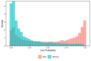
Figure 2: Distribution of Like Probabilities

In Table 4, we report summary statistics for the sample used in the numerical experiments (standard deviations in parenthesis).

Table 4: Descriptives of Instance

	$N$	Score	Potentials	Backlog	Like Prob.
Women	173	5.289	73.23	0.120	0.203
		(2.454)	(15.032)	(0.152)	(0.247)
Men	113	2.618	97.461	0.012	0.536
		(1.463)	(21.680)	(0.026)	(0.368)

11.2 Perfect Matching (PM)

The Perfect Matching heuristic solves, in each period $t\in[T]$, the following problem:

$$\begin{split}\max\quad&\;\sum_{\ell\in I\cup J}\sum_{\ell^{\prime}\in\mathcal{P}_{\ell}}y_{\ell\ell^{\prime}}^{t}\phi^{t}_{\ell\ell^{\prime}}+\frac{1}{2}w_{\ell\ell^{\prime}}^{t}\beta^{t}_{\ell\ell^{\prime}}\\ st.\quad&y_{\ell\ell^{\prime}}^{t}\leq\mathbbm{1}_{\left\{\ell^{\prime}\in\mathcal{B}_{\ell}^{t}\right\}},\hskip 87.00009pt\text{for every}\ \ell^{\prime}\in\mathcal{P}^{t}_{\ell},\ell\in I\cup J\\ &x_{\ell\ell^{\prime}}^{t}+y_{\ell\ell^{\prime}}^{t}\leq 1,\hskip 92.0001pt\text{for every}\ \ell^{\prime}\in\mathcal{P}^{t}_{\ell},\ell\in I\cup J\\ &\sum_{\ell^{\prime}\in\mathcal{P}_{\ell}^{t}}x_{\ell\ell^{\prime}}^{t}+y_{\ell\ell^{\prime}}^{t}\leq K_{\ell},\hskip 74.00005pt\text{for every}\ \ell\in I\cup J\\ &w_{\ell\ell^{\prime}}^{t}\leq x_{\ell\ell^{\prime}}^{t},\;w_{\ell\ell^{\prime}}^{t}\leq x_{\ell^{\prime}\ell}^{t},\;w_{\ell\ell^{\prime}}^{t}=w_{\ell^{\prime}\ell}^{t},\hskip 18.00005pt\text{for every}\ \ell^{\prime}\in\mathcal{P}^{t}_{\ell},\ell\in I\cup J\\ &x_{\ell\ell^{\prime}}^{t},y_{\ell\ell^{\prime}}^{t},w_{\ell\ell^{\prime}}^{t}\in\left\{0,1\right\},\hskip 84.00006pt\text{for every}\ \ell^{\prime}\in\mathcal{P}^{t}_{\ell},\ell\in I\cup J,\end{split}$$ (25)

Then, set $S_{\ell}^{t}=\left\{\ell^{\prime}\in\mathcal{P}_{\ell}^{t}:x_{\ell\ell^{\prime}}^{t}=1\text{ or }y_{\ell\ell^{\prime}}^{t}=1\right\}$ for each $\ell\in I\cup J$. Note that, if there is no initial backlog, then the problem can be re-formulated as:

$$\begin{split}\max\quad&\;\sum_{e\in\vec{E}_{I}}w_{e}^{t}\beta^{t}_{e}\\ st.\quad&\sum_{e\in\vec{E}_{I}:\ell\in e}w_{e}^{t}\leq K_{\ell},\hskip 60.00009pt\text{for every}\ \ell\in I\cup J\\ &\sum_{t\in[T]}w_{e}^{t}\leq 1,\hskip 74.00005pt\text{for every}e\in\vec{E}_{I}\\ &w_{e}^{t}\in\left\{0,1\right\},\hskip 75.0001pt\text{for every}\ e\in\vec{E}_{I},\end{split}$$ (26)

where the second constraint ensures that each edge is used at most once, i.e., that no two users see each other more than once. This is captured in the previous formulation through the set of potentials $\mathcal{P}_{\ell}^{t}$.

11.3 Dating Heuristic (DH)

For each period $t\in[T]$, DH considers two steps:

1. Optimization: this step involves solving the following linear program:

   $$\begin{split}\max\quad&\;\sum_{\tau=t}^{t+1}\sum_{\ell\in I\cup J}\sum_{\ell^{\prime}\in\mathcal{P}^{t}_{\ell}}y_{\ell\ell^{\prime}}^{\tau}\phi^{\tau}_{\ell\ell^{\prime}}+\frac{1}{2}\cdot w_{\ell\ell^{\prime}}^{\tau}\phi^{\tau}_{\ell\ell^{\prime}}\phi^{\tau}_{\ell^{\prime}\ell}\\ \text{s.t.}\quad&\;\sum_{\tau=t}^{t^{\prime}}y_{\ell\ell^{\prime}}^{\tau}\leq\mathbbm{1}_{\left\{\ell^{\prime}\in\mathcal{B}^{t}_{\ell}\right\}}+\sum_{\tau=t}^{t^{\prime}-1}(x_{\ell^{\prime}\ell}^{\tau}-w_{\ell\ell^{\prime}}^{\tau})\phi^{\tau}_{\ell^{\prime}\ell},\hskip 10.00002pt\text{for every }\ell^{\prime}\in\mathcal{P}^{t}_{\ell},\ell\in I\cup J,t^{\prime}\in[t,t+1],\\ &\;\sum_{\tau=t}^{t+1}x_{\ell\ell^{\prime}}^{\tau}+y_{\ell\ell^{\prime}}^{\tau}\leq 1,\hskip 99.00008pt\text{for every }\ell^{\prime}\in\mathcal{P}^{t}_{\ell},\ell\in I\cup J,\\ &\;\sum_{\ell^{\prime}}x_{\ell\ell^{\prime}}^{\tau}+y_{\ell\ell^{\prime}}^{\tau}\leq K_{\ell},\hskip 97.0001pt\text{for every }\ell\in I\cup J,t\in[t,t+1],\\ &\;w_{\ell\ell^{\prime}}^{\tau}\leq x_{\ell\ell^{\prime}}^{\tau},\;w_{\ell\ell^{\prime}}^{\tau}\leq x_{\ell^{\prime}\ell}^{\tau},\;w_{\ell\ell^{\prime}}^{\tau}=w_{\ell^{\prime}\ell}^{\tau},\hskip 43.00009pt\text{for every }\ell^{\prime}\in\mathcal{P}^{t}_{\ell},\ell\in I\cup J,t\in[t,t+1],\\ &\;x_{\ell\ell^{\prime}}^{\tau},\;y_{\ell\ell^{\prime}}^{\tau},w_{\ell\ell^{\prime}}^{\tau}\in\left[0,1\right],\hskip 87.00009pt\text{for every }\ell^{\prime}\in\mathcal{P}^{t}_{\ell},\ell\in I\cup J,t\in[t,t+1].\end{split}$$ (27)

   The decision variables $y_{\ell,\ell^{\prime}}^{t}$ and $x_{\ell,\ell^{\prime}}^{t}$ represent whether $\ell$ sees profile $\ell^{\prime}$ in period $t$ as part of a backlog and to initiate a sequential match, respectively. The objective is to maximize the expected number of matches obtained in periods $\left\{t,t+1\right\}$, including sequential matches (first term in the objective) and simultaneous matches (second term in the objective). The first constraint defines $y$ and captures the evolution of the backlog. The second captures that a profile can be shown at most once, while the third constraint considers the assortment size. Finally, the last constraint captures the definition of $w_{\ell,\ell^{\prime}}^{t}$, which accounts for simultaneous matches between $\ell$ and $\ell^{\prime}$ in period $t$.

2. Rounding: since the optimal decisions $x^{*,t},y^{*,t},w^{*,t}$ of (27) may be fractional, this step involves rounding them in order to decide the assortments to show in the current period. Specifically, the rounding process starts by adding to $S_{\ell}^{t}$ the profiles for which $y_{\ell,\ell^{\prime}}^{t}>0$ (in decreasing order). Then, if there is space left in the assortment, the rounding procedure add to $S_{\ell}^{t}$ the profiles for which $x_{\ell,\ell^{\prime}}^{t}>0$ (in decreasing order), making sure that the assortment size constraints are satisfied.

Notice that these two steps consider the current set of potentials $\mathcal{P}_{\ell}^{t}$ and backlog $\mathcal{B}_{\ell}^{t}$ for each user $\ell\in I\cup J$. Then, at the end of each period the sets of potentials and the backlogs must be updated considering the assortments shown and the like/dislike decisions. Specifically,

$$\mathcal{P}_{\ell}^{t+1}=\mathcal{P}_{\ell}^{t}\setminus\left(S_{\ell}^{t}\cup\left\{\ell^{\prime}\in\mathcal{P}_{\ell}^{t}:\ell\in S_{\ell^{\prime}}^{t},\;\Phi_{\ell^{\prime}\ell}^{t}=0\right\}\right),\quad\mathcal{B}_{\ell}^{t+1}=\left(\mathcal{B}_{\ell}^{t}\cup\left\{\ell^{\prime}\in\mathcal{P}_{\ell}^{t}:\ell\in S_{\ell^{\prime}}^{t},\;\Phi_{\ell^{\prime}\ell}^{t}=1\right\}\right)\setminus S_{\ell}^{t}.$$

This procedure in formally described in Algortihm 3.

Algorithm 3 Dating Heuristic (DH)

1:An instance for a two-sided assortment problem.

2:A feasible assortment.

3:for $t\in[T]$ do

4:     Solve (27) and keep $x^{*,t},\,y^{*,t}$.

5:     

For each user $\ell$, sequentially add profiles $\ell^{\prime}$ for which $y_{\ell,\ell^{\prime}}^{*,t}>0$ until the assortment size is reached. If there is space left in the assortment, add profiles $\ell^{\prime}$ for which $x_{\ell,\ell^{\prime}}^{*,t}>0$ until the assortment size is reached.

6:     Update potentials and backlogs.

11.4 Proof of Proposition 6.1

Consider a platform design with one-directional matches and sequential matches. Then, the problem that the DH algorithm solves can be formulated as:

$$\begin{split}\max\quad&\quad\sum_{j\in J}\sum_{i\in\mathcal{P}_{j}}y_{j,i}\cdot\phi^{2}_{j,i}\\ st.\quad&\quad y_{j,i}\leq x_{i,j}\cdot\phi^{1}_{i,j},\hskip 50.00008pt\forall i\in I,j\in\mathcal{P}_{i}\\ &\quad\sum_{j\in\mathcal{P}_{i}}x_{i,j}\leq K_{i},\hskip 52.00005pt\forall i\in I\\ &\quad\sum_{i\in\mathcal{P}_{j}}y_{j,i}\leq K_{j},\hskip 52.00005pt\forall j\in J\\ &\quad x_{i,j}\in\left\{0,1\right\},\;y_{j,i}\in[0,1],\;\quad\forall(i,j)\in I\times J\end{split}$$ (28)

To show that Algorithm 1 provides a lower bound for the performance of DH, it is enough to show Lemmas 11.1 and 11.3. The first lemma states that we can construct a feasible solution for Problem 28 using the solution from Algorithm 1. The second lemma states that, given two feasible solutions of Problem 28, the one leading with the highest objective also leads to a higher objective in Problem 3.3. Then, since DH uses the optimal solution of Problem 28 in the first period, we know that the objective function is higher than for the solution obtained from Algorithm 1 and, by Lemma 11.3, we directly obtain that the solution from DH leads to a higher expected number of matches than that of Algorithm 1.

Lemma 11.1

The solution of Algorithm 1 can be used to construct a feasible solution of DH.

Proof 11.2

Proof of Lemma 11.1. Let $\mathbf{\hat{x}}=\left\{\hat{x}_{e}\right\}_{e\in\vec{E}_{I}}$ be the first period decisions obtained from Algorithm 1, and let $\mathbf{\hat{y}}=\left\{\hat{y}_{e}\right\}_{e\in\vec{E}_{J}}$ be such that

$$\hat{y}_{j,i}=\sum_{\mathbf{B}\subseteq\vec{E}_{I}}\mathbbm{1}_{\left\{i\in S_{j}(\mathbf{B})\right\}}\cdot\text{I\kern-1.49994ptP}_{\mathbf{\hat{x}}}(\mathbf{B})$$

$S_{j}(\mathbf{B})$ is the set of users displayed to $j$ in the second period given a realized backlog $B$. More specifically, $S_{j}(\mathbf{B})$ is the set of $K_{j}$ (or less) users in the backlog $B_{j}$ with the highest probability of generating a match, i.e., $S_{j}(\mathbf{B})=\argmax\left\{S:\sum_{i\in S}\phi^{2}_{j,i}\;:\;S\subseteq\mathbf{B},\left|S\right|\leq K_{j}\right\}$.

From the definition of $P^{1}$, it is direct that $\sum_{j\in\mathcal{P}_{i}}\hat{x}_{i,j}\leq K_{i}$ for all $i\in I$. In addition, note that

$$\begin{split}\hat{y}_{j,i}&=\sum_{\mathbf{B}\subseteq\vec{E}_{I}}\mathbbm{1}_{\left\{i\in S_{j}(\mathbf{B})\right\}}\cdot\text{I\kern-1.49994ptP}_{\mathbf{\hat{x}}}(\mathbf{B})\\ &=\sum_{\mathbf{B}^{\prime}\subseteq\vec{E}_{I}\setminus(i,j)}\mathbbm{1}_{\left\{i\in S_{j}(\mathbf{B}^{\prime}\cup(i,j))\right\}}\cdot\text{I\kern-1.49994ptP}_{\mathbf{\hat{x}}}(\mathbf{B}^{\prime}\cup(i,j))\\ &=\sum_{\mathbf{B}^{\prime}\subseteq\vec{E}_{I}\setminus(i,j)}\mathbbm{1}_{\left\{i\in S_{j}(\mathbf{B}^{\prime}\cup(i,j))\right\}}\cdot\text{I\kern-1.49994ptP}_{\mathbf{\hat{x}}}((i,j))\text{I\kern-1.49994ptP}_{\mathbf{\hat{x}}}(\mathbf{B}^{\prime})\\ &=\hat{x}_{i,j}\cdot\phi_{i,j}\cdot\sum_{\mathbf{B}^{\prime}\subseteq\vec{E}_{I}\setminus(i,j)}\mathbbm{1}_{\left\{i\in S_{j}(\mathbf{B}^{\prime}\cup(i,j))\right\}}\cdot\text{I\kern-1.49994ptP}_{\mathbf{\hat{x}}}(\mathbf{B}^{\prime})\\ &\leq\hat{x}_{i,j}\cdot\phi_{i,j}^{1}\end{split}$$

Finally, notice that

$$\begin{split}\sum_{i\in\mathcal{P}_{j}}\hat{y}_{j,i}&=\sum_{i\in\mathcal{P}_{j}}\sum_{\mathbf{B}\subseteq\vec{E}_{I}}\mathbbm{1}_{\left\{i\in S_{j}(\mathbf{B})\right\}}\cdot\text{I\kern-1.49994ptP}_{\mathbf{\hat{x}}}(\mathbf{B})\\ &=\sum_{\mathbf{B}\subseteq\vec{E}_{I}}\sum_{i\in\mathcal{P}_{j}}\mathbbm{1}_{\left\{i\in S_{j}(\mathbf{B})\right\}}\cdot\text{I\kern-1.49994ptP}_{\mathbf{\hat{x}}}(\mathbf{B})\\ &=\sum_{\mathbf{B}\subseteq\vec{E}_{I}}\left[\sum_{k=0}^{K_{j}-1}k\cdot\text{I\kern-1.49994ptP}_{\mathbf{\hat{x}}}\left(\left|B_{j}\right|=k\right)+K_{j}\cdot\text{I\kern-1.49994ptP}_{\mathbf{\hat{x}}}\left(\left|B_{j}\right|\geq K_{j}\right)\right]\cdot\text{I\kern-1.49994ptP}_{\mathbf{\hat{x}}}(\mathbf{B})\\ &\leq\sum_{\mathbf{B}\subseteq\vec{E}_{I}}K_{j}\cdot\text{I\kern-1.49994ptP}_{\mathbf{\hat{x}}}(\mathbf{B})\\ &=K_{j}\end{split}$$

Hence, we conclude that the solution $\mathbf{\hat{x}},\mathbf{\hat{y}}$ is feasible for Problem (28).

Lemma 11.3

Given two feasible solutions $(\mathbf{x},\mathbf{y})$ and $(\mathbf{x}^{\prime},\mathbf{y}^{\prime})$ of Problem 28 such that

$$\sum_{j\in J}\sum_{i\in\mathcal{P}_{j}}y_{j,i}\cdot\phi_{j,i}^{2}\leq\sum_{j\in J}\sum_{i\in\mathcal{P}_{j}}y_{j,i}^{\prime}\cdot\phi_{j,i}^{2},$$

then

$$\mathbb{E}_{\mathbf{\mathcal{B}}\sim\phi^{1}\mathbf{x}}\left[f(\mathbf{\mathcal{B}})\right]\leq\mathbb{E}_{\mathbf{\mathcal{B}}\sim\phi^{1}\mathbf{x}^{\prime}}\left[f(\mathbf{\mathcal{B}})\right].$$

Proof 11.4

Proof of Lemma 11.3. First, recall that

$$\mathbb{E}_{\mathbf{\mathcal{B}}\sim\phi^{1}\mathbf{x}}\left[f(\mathbf{\mathcal{B}})\right]=\sum_{\mathbf{B}\subseteq\vec{E}_{I}}f(\mathbf{B})\cdot\text{I\kern-1.49994ptP}_{\mathbf{x}}(\mathbf{B}).$$

Consider a fixed $\mathbf{x}$, and let $f_{j}(\mathbf{B})$ be the expected number of matches obtained by $j$ in $f$, i.e., $f(\mathbf{B})=\sum_{j\in J}f_{j}(\mathbf{B})$, with $\mathbf{B}\sim\phi^{1}\mathbf{x}$. Note that, given a realized backlog $B$, $f_{j}$ and $f_{j^{\prime}}$ are independent for any $j,j^{\prime}\in J$. In addition, notice that $f_{j}(\mathbf{B})$ can be formulated as the solution of the following optimization problem:

$$\begin{split}\max\quad&\quad\sum_{i\in\mathcal{P}_{j}}z_{i}\cdot\phi_{j,i}^{2}\\ st.\quad&\quad\sum_{i\in\mathcal{P}_{j}}z_{i}\leq K_{j}\\ &\quad z_{i}\leq\mathbbm{1}_{\left\{i\in B_{j}\right\}},\quad\forall i\in\mathcal{P}_{j}\\ &\quad z_{i}\in\left\{0,1\right\},\quad\forall i\in\mathcal{P}_{j}.\end{split}$$

Let $\mathbf{z}^{*}$ be the optimal solution of this problem. It is easy to see that $z_{i}^{*}=1$ if and only if $i\in S_{j}(\mathbf{B})$, so we can re-write $z_{i}^{*}=\mathbbm{1}_{\left\{i\in S_{j}(\mathbf{B})\right\}}$. Then,

$$\begin{split}\mathbb{E}_{\mathbf{\mathcal{B}}\sim\phi^{1}\mathbf{x}}\left[f_{j}(\mathbf{\mathcal{B}})\right]&=\sum_{\mathbf{B}\subseteq\vec{E}_{I}}\left[\sum_{i\in\mathcal{P}_{j}}z_{i}^{*}(\mathbf{B})\cdot\phi_{j,i}^{2}\right]\cdot\text{I\kern-1.49994ptP}_{\mathbf{x}}(\mathbf{B})\\ &=\sum_{\mathbf{B}\subseteq\vec{E}_{I}}\left[\sum_{i\in\mathcal{P}_{j}}\mathbbm{1}_{\left\{i\in S_{j}(\mathbf{B})\right\}}\cdot\phi_{j,i}^{2}\right]\cdot\text{I\kern-1.49994ptP}_{\mathbf{x}}(\mathbf{B})\\ &=\sum_{i\in\mathcal{P}_{j}}\sum_{\mathbf{B}\subseteq\vec{E}_{I}}\mathbbm{1}_{\left\{i\in S_{j}(\mathbf{B})\right\}}\cdot\text{I\kern-1.49994ptP}_{\mathbf{x}}(\mathbf{B})\cdot\phi_{j,i}^{2}\\ &=\sum_{i\in\mathcal{P}_{j}}y_{j,i}\cdot\phi_{j,i}^{2}\\ \end{split}$$

where the last equality follows from the construction in the proof of Lemma 11.1 (we add the dependence on $B$ to avoid confusion). Then, if we know there are two feasible solutions $(\mathbf{x},\mathbf{y})$ and $(\mathbf{x}^{\prime},\mathbf{y}^{\prime})$ such that the latter leads to a higher objective of Problem (28), we know that

$$\mathbb{E}_{\mathbf{\mathcal{B}}\sim\phi^{1}\mathbf{x}}\left[f_{j}(\mathbf{\mathcal{B}})\right]=\sum_{i\in\mathcal{P}_{j}}y_{j,i}\cdot\phi_{j,i}^{2}\leq\sum_{i\in\mathcal{P}_{j}}y^{\prime}_{j,i}\cdot\phi_{j,i}^{2}=\mathbb{E}_{\mathbf{\mathcal{B}}\sim\phi^{1}\mathbf{x}^{\prime}}\left[f_{j}(\mathbf{\mathcal{B}})\right]$$

concluding our proof.

References

- Adamczyk (2011) Adamczyk M (2011) Improved analysis of the greedy algorithm for stochastic matching. Information Processing Letters 111(15):731–737.
- Agrawal et al. (2010) Agrawal S, Ding Y, Saberi A, Ye Y (2010) Correlation robust stochastic optimization. Proceedings of the twenty-first annual ACM-SIAM symposium on Discrete Algorithms, 1087–1096 (SIAM).
- Aouad and Saban (2022) Aouad A, Saban D (2022) Online assortment optimization for two-sided matching platforms. Management Science 0(0).
- Arnosti and Shi (2020) Arnosti N, Shi P (2020) Design of lotteries and wait-lists for affordable housing allocation. Management Science 66(6):2291–2307.
- Ashlagi et al. (2022) Ashlagi I, Krishnaswamy A, Makhijani R, Saban D, Shiragur K (2022) Technical note - assortment planning for two-sided sequential matching markets. Operations Research 70(5):2784–2803.
- Bansal et al. (2012) Bansal N, Gupta A, Li J, Mestre J, Nagarajan V, Rudra A (2012) When lp is the cure for your matching woes: Improved bounds for stochastic matchings. Algorithmica 63:733–762.
- Berbeglia and Joret (2015) Berbeglia G, Joret G (2015) Assortment Optimisation Under a General Discrete Choice Model: A Tight Analysis of Revenue-Ordered Assortments.
- Besbes et al. (2021) Besbes O, Castro F, Lobel I (2021) Surge pricing and its spatial supply response. Management Science 67(3):1350–1367.
- Besbes et al. (2023) Besbes O, Fonseca Y, Lobel I, Zheng F (2023) Signaling competition in two-sided markets.
- Blanchet et al. (2016) Blanchet J, Gallego G, Goyal V (2016) A Markov chain approximation to choice modeling. Operations Research 64(4):886–905.
- Brubach et al. (2021) Brubach B, Grammel N, Ma W, Srinivasan A (2021) Improved guarantees for offline stochastic matching via new ordered contention resolution schemes. Advances in Neural Information Processing Systems 34:27184–27195.
- Calinescu et al. (2011) Calinescu G, Chekuri C, Pal M, Vondrák J (2011) Maximizing a monotone submodular function subject to a matroid constraint. SIAM Journal on Computing 40(6):1740–1766.
- Caro and Gallien (2007) Caro F, Gallien J (2007) Dynamic assortment with demand learning for seasonal consumer goods. Management Science 53(2):276–292.
- Chekuri et al. (2010) Chekuri C, Vondrák J, Zenklusen R (2010) Dependent randomized rounding via exchange properties of combinatorial structures. 2010 IEEE 51st Annual Symposium on Foundations of Computer Science, 575–584 (IEEE).
- Chen et al. (2009) Chen N, Immorlica N, Karlin AR, Mahdian M, Rudra A (2009) Approximating matches made in heaven. Automata, Languages and Programming, 266–278 (Springer Berlin Heidelberg).
- Costello et al. (2012) Costello KP, Tetali P, Tripathi P (2012) Stochastic matching with commitment. Automata, Languages, and Programming: 39th International Colloquium, ICALP 2012, Warwick, UK, July 9-13, 2012, Proceedings, Part I 39, 822–833 (Springer).
- Davis et al. (2014) Davis JM, Gallego G, Topaloglu H (2014) Assortment Optimization Under Variants of the Nested Logit Model. Operations Research 62(2):250–273.
- Erdős and Rényi (1964) Erdős P, Rényi A (1964) On random matrices. Publ. Math. Inst. Hungarian Academy of Sciences 8:455–461.
- Erdős and Rényi (1968) Erdős P, Rényi A (1968) On random matrices ii. Studia Sci. Math. Hungar 3:459–464.
- Farias et al. (2013) Farias VF, Jagabathula S, Shah D (2013) A Nonparametric Approach to Modeling Choice with Limited Data. Management Science 59(2):305–322.
- Feldman et al. (2009) Feldman J, Mehta A, Mirrokni V, Muthukrishnan S (2009) Online stochastic matching: Beating 1-1/e. 2009 50th Annual IEEE Symposium on Foundations of Computer Science, 117–126 (IEEE).
- Fisher et al. (1978) Fisher ML, Nemhauser GL, Wolsey L (1978) An analysis of approximations for maximizing submodular set functions–ii. Polyhedral combinatorics .
- Gamlath et al. (2019) Gamlath B, Kale S, Svensson O (2019) Beating greedy for stochastic bipartite matching. Proceedings of the Thirtieth Annual ACM-SIAM Symposium on Discrete Algorithms, 2841–2854 (SIAM).
- Gandhi et al. (2006) Gandhi R, Khuller S, Parthasarathy S, Srinivasan A (2006) Dependent rounding and its applications to approximation algorithms. Journal of the ACM (JACM) 53(3):324–360.
- Golrezaei et al. (2014) Golrezaei N, Nazerzadeh H, Rusmevichientong P (2014) Real-Time Optimization of Personalized Assortments. Management Science 60(6):1532–1551.
- Goyal and Udwani (2023) Goyal V, Udwani R (2023) Online matching with stochastic rewards: Optimal competitive ratio via path-based formulation. Operations Research 71(2):563–580.
- Halaburda et al. (2018) Halaburda H, Piskorski MJ, Yildirim P (2018) Competing by Restricting Choice: The Case of Search Platforms. Management Science 64(8):3574–3594.
- Hikima et al. (2021) Hikima Y, Akagi Y, Kim H, Kohjima M, Kurashima T, Toda H (2021) Integrated optimization of bipartite matching and its stochastic behavior: New formulation and approximation algorithm via min-cost flow optimization. Proceedings of the AAAI Conference on Artificial Intelligence, volume 35, 3796–3805.
- Immorlica et al. (2022) Immorlica N, Lucier B, Manshadi V, Wei A (2022) Designing approximately optimal search on matching platforms. Management Science Forthcoming.
- Jeloudar et al. (2021) Jeloudar M, Lo I, Pollner T, Saberi A (2021) Decentralized matching in a probabilistic environment. Proceedings of the 22nd ACM Conference on Economics and Computation, 635–653.
- Kanoria and Saban (2021) Kanoria Y, Saban D (2021) Facilitating the search for partners on matching platforms. Management Science 67(10):5990–6029.
- Karp et al. (1990) Karp R, Vazirani U, Vazirani V (1990) An optimal algorithm for online bipartite matching. Proceedings of the 22nd Annual ACM Symposium on Theory of Computinh.
- Kök et al. (2015) Kök A, Fisher M, Vaidyanathan R (2015) Retail Supply Chain Management: Quantitative Models and Empirical Studies, 175–236 (Springer US).
- Lee et al. (2009) Lee J, Sviridenko M, Vondrák J (2009) Submodular maximization over multiple matroids via generalized exchange properties. International Workshop on Approximation Algorithms for Combinatorial Optimization, 244–257 (Springer).
- Manshadi and Rodilitz (2022) Manshadi V, Rodilitz S (2022) Online policies for efficient volunteer crowdsourcing. Management Science 68(9):6572–6590.
- Manshadi et al. (2022) Manshadi V, Rodilitz S, Saban D, Suresh A (2022) Online algorithms for matching platforms with multi-channel traffic.
- Manshadi et al. (2012) Manshadi VH, Gharan SO, Saberi A (2012) Online stochastic matching: Online actions based on offline statistics. Mathematics of Operations Research 37(4):559–573.
- Mehta and Panigrahi (2012) Mehta A, Panigrahi D (2012) Online matching with stochastic rewards. 2012 IEEE 53rd Annual Symposium on Foundations of Computer Science, 728–737 (IEEE).
- Mehta et al. (2013) Mehta A, et al. (2013) Online matching and ad allocation. Foundations and Trends® in Theoretical Computer Science 8(4):265–368.
- Rios et al. (2023) Rios I, Saban D, Zheng F (2023) Improving match rates in dating markets through assortment optimization. Manufacturing & Service Operations Management 25(4):1304–1323.
- Rochet and Tirole (2003) Rochet JC, Tirole J (2003) Two-Sided Markets. Journal of the European Economic Association 990–1029.
- Rusmevichientong et al. (2010) Rusmevichientong P, Shen ZJM, Shmoys DB (2010) Dynamic Assortment Optimization with a Multinomial Logit Choice Model and Capacity Constraint. Operations Research 58(6):1666–1680.
- Rusmevichientong et al. (2014) Rusmevichientong P, Shmoys D, Tong C, Topaloglu H (2014) Assortment optimization under the multinomial logit model with random choice parameters. Production and Operations Management 23(11):2023–2039.
- Rusmevichientong et al. (2020) Rusmevichientong P, Sumida M, Topaloglu H (2020) Dynamic assortment optimization for reusable products with random usage durations. Management Science 66(7):2820–2844.
- Sauré and Zeevi (2013) Sauré D, Zeevi A (2013) Optimal Dynamic Assortment Planning with Demand Learning. Manufacturing & Service Operations Management 15(3):387–404.
- Shi (2022a) Shi P (2022a) Optimal matchmaking strategy in two-sided marketplaces. Management Science 0(0):null.
- Shi (2022b) Shi P (2022b) Optimal priority-based allocation mechanisms. Management Science 68(1):171–188.
- Talluri and van Ryzin (2004) Talluri K, van Ryzin G (2004) Revenue Management Under a General Discrete Choice Model of Consumer Behavior. Management Science 50(1):15–33.
- Torrico et al. (2021) Torrico A, Carvalho M, Lodi A (2021) Multi-agent assortment optimization in sequential matching markets.
- Vondrák (2008) Vondrák J (2008) Optimal approximation for the submodular welfare problem in the value oracle model. Proceedings of the 40th Annual ACM Symposium on the Theory of Computing (STOC), 67–74.
- Wang and Sahin (2018) Wang R, Sahin O (2018) The Impact of Consumer Search Cost on Assortment Planning and Pricing. Management Science 64(8):3649–3666.