Adapt and Decompose: Efficient Generalization of Text-to-SQL via Domain Adapted Least-To-Most Prompting

Abstract

Cross-domain and cross-compositional generalization of Text-to-SQL semantic parsing is a challenging task. Existing Large Language Model (LLM) based solutions rely on inference-time retrieval of few-shot exemplars from the training set to synthesize a run-time prompt for each Natural Language (NL) test query. In contrast, we devise an algorithm which performs offline sampling of a minimal set-of few-shots from the training data, with complete coverage of SQL clauses, operators and functions, and maximal domain coverage within the allowed token length. This allows for synthesis of a fixed Generic Prompt (GP), with a diverse set-of exemplars common across NL test queries, avoiding expensive test time exemplar retrieval. We further auto-adapt the GP to the target database domain (DA-GP), to better handle cross-domain generalization; followed by a decomposed Least-To-Most-Prompting (LTMP-DA-GP) to handle cross-compositional generalization. The synthesis of LTMP-DA-GP is an offline task, to be performed one-time per new database with minimal human intervention. Our approach demonstrates superior performance on the KaggleDBQA dataset, designed to evaluate generalizability for the Text-to-SQL task. We further showcase consistent performance improvement of LTMP-DA-GP over GP, across LLMs and databases of KaggleDBQA, highlighting the efficacy and model agnostic benefits of our prompt based adapt and decompose approach.

1 Introduction

Recently, Large Language Models (LLMs) such as GPT3(Brown et al., 2020a), Codex(Chen et al., 2021b), PaLMChowdhery et al. (2022), pretrained with massive volumes of data have shown improved performance for multiple reasoning tasks using in-context learning (Brown et al., 2020b; Huang and Chang, 2022), including program synthesis (Austin et al., 2021; Jain et al., 2021; Nijkamp et al., 2022) and semantic parsing (Shin and Durme, 2021; Drozdov et al., 2022; Shin and Durme, 2021; Shin et al., 2021). There are a few recent approaches where LLMs are specifically used for Text-to-SQL semantic parsing in a (i) zero-shot setting (Rajkumar et al., 2022a; Chang and Fosler-Lussier, 2023; Nan et al., 2023) where only the test Natural Language (NL) query constitutes the prompt, (ii) few-shot setting where exemplars similar to the test query in the target domain are retrieved from the available training data and appended to the test NL query to constitute the prompt (Poesia et al., 2022a; Chang and Fosler-Lussier, 2023; Nan et al., 2023; An et al., 2023). For this setting the available NL-SQL pairs would belong to domains that are different from the target database domain (iii) few-shot setting where exemplars are sampled NL-SQL queries available for the target-domain with maximum coverage of compositions (Rajkumar et al., 2022a; Qiu et al., 2022; Hosseini et al., 2022; Yang et al., 2022; Chang and Fosler-Lussier, 2023). In this paper, we are mainly interested in (ii) i.e. cross-domain generalization along with the scenario where the test queries may not have the set-of compositions covered in the training data (cross-composition generalizability). Moreover, considering a purely cross-domain setting, as opposed to (iii) above, we assume NO availability of exemplars belonging to the target databases. One solution to this setting is manual synthesis of few-shots for every new target database from scratch. However, this process is very tedious, time-consuming and also does not ensure diversity in the few-shots, with good coverage of SQL operators. Thus, there is a need for an efficient approach which can exploit available NL-SQL pairs from distinct domains, to intelligently sample few-shots and design prompts.

Synchromesh (Poesia et al., 2022a) and Nan et al. (2023); An et al. (2023) have a similar setting, except they retrieve exemplars during run-time (during inference) by selecting NL queries as exemplars with similarity based on (a) NL query semantics (Nan et al., 2023) or (b) target SQLs (Target Similarity Tuning) Poesia et al. (2022a) or (c) LLM generated ‘skill’ based NL representation, focusing on program compositions and ignoring the surface NL forms An et al. (2023). This reliance on inference-time retrieval of similar few-shots from the available data to build a run-time prompt and generate SQL for a test NL query, results in a less efficient solution. As opposed to this, we devise an algorithm which samples a minimal set-of few-shots from the training data ensuring complete coverage of SQL clauses, operators and functions and maximum coverage of database domains, which fits into the token length restriction. We append these few-shots with the out-of-distribution test NL query to define what we term as a Generic Prompt (GP), which is further used to generate the corresponding SQL. The GP is generated offline and is common across distinct test queries, resulting in a more time-efficient solution obviating the need for real time retrieval. We further auto-adapt the GP to (a) the target database domain, and refer to it as domain adapted GP (DA-GP), to better handle cross-domain generalization, (b) decompose it into a Least-To-Most-Prompting approach Zhou et al. (2022) (LTMP-GP) to better handle cross-compositional generalization, and (c) combine the approaches (a) and (b) to exploit their complementary benefits (LTMP-DA-GP). In line with our motivation, formation of LTMP-DA-GP is an efficient solution, as it is an offline task to be performed one-time per new database and is mostly programmatic with minimal human intervention (only needed for validation of prompts). We further demonstrate a consistent performance improvement of (a) and (b) over the base GP and (c) over (a) and (b) on the databases of Kaggle-DBQA dataset Lee et al. (2021a), designed to evaluate the generalizability of the Text-to-SQL task using distinct LLMs. Moreover, our approach not only yields an efficient solution, but also yields best performance for the used LLMs on KaggleDBQA. Following are our main contributions:

• To the best of our knowledge, apart from Nan et al. (2023) ours is the only approach to implement offline programmatic prompt generation ensuring diversity of samples for NL-to-SQL task. Moreover, as opposed to Nan et al. (2023), our GP based sampling technique guarantees complete coverage of SQL operators and maximum converge of database domains.

• Ours is the first approach of programmatic domain-adaptation of prompt, consistently showcasing performance improvement across multiple Kaggle-DBQA databases validating NL-to-SQL domain generalization capability.

• Ours is the first approach applying Least-to-Most-Prompting Zhou et al. (2022) for compositional generalization of complex NL-to-SQL task, showcasing consistent performance improvement across LLMs.

• As compared to existing similarity based exemplar sampling approaches (Poesia et al., 2022b; Chang and Fosler-Lussier, 2023; An et al., 2023), our approach of offline prompts synthesis proves to be more efficient.

• Our pipeline yields the best performance on the KaggleDBQA dataset, reported in the literature for the used LLMs.

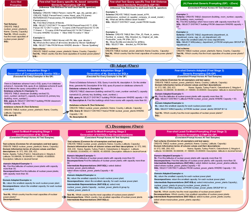
Figure 1: Comparison of our Approach (A) GP (B) DA-GP (Stage 1, 2, 3) and (C) LTMP-DA-GP (Stage 1, 2, 3) with Prior Zero-shot, Query-Similarity based Few-shot Approaches

2 Datasets

Spider Gan et al. (2022): Is a large-scale, complex, and cross-domain Text-to-SQL benchmark dataset with a total of 200 databases (140, 20, 40 in the training, development and test splits with 7000, 1034, and 2147 Text-to-SQL pairs). We use state-of-the-art models trained on Spider to benchmark performance of our approach against supervised approaches. We also use the training split of Spider to sample the exemplars, which serve as few-shots in our prompt (Section 4).

Spider-CG Gan et al. (2022): This dataset is designed for evaluating Text-to-SQL compositional generalization performance. To synthesize this dataset, Text-to-SQL pairs from Spider-Train are transformed to corresponding sub-sentences and NatSQL pairs to form Spider-SS dataset. The sub-sentences are obtained using a sentence-split algorithm and the corresponding NatSQL, which is an intermediate representation of SQL, is manually annotated. We use the Spider-SS for the Least-To-Most-Prompting (LTMP) experiment, by retrieving the NL query decompositions in terms of sub-sentences and the corresponding intermediate NatSQL representations for few-shots sampled from Spider-Train, to synthesize prompts for each stage of LTMP (Section 4.4).

Kaggle-DBQA Lee et al. (2021b): This is a cross-domain Text-to-SQL evaluation dataset with real world databases (DB). It covers a total of 8 DBs, viz. (i) Nuclear (10,22), (ii) Crime (9,18), (iii) Pesticide (16, 34), (iv) MathScore (9,19), (v) Baseball (12,27), (vi) Fires (12, 25), (vii) WhatCD (13,28), and (viii) Soccer (6,12), indicating fine-tuning and test examples, respectively. As we assume a purely cross-domain setting with no availability of in-domain few-shots, we do not use the fine-tuning samples but use only the test samples to evaluate our proposed LLM based pipelines. We prefer Kaggle-DBQA over other cross-domain and composition evaluation datasets such as spider-CG Gan et al. (2022), because it is a real-web dataset and contains fewer test queries allowing us to showcase the efficacy of our approach using commercial LLMs with low cost overheads.

3 Large Language Models (LLMs)

The literature has demonstrated state-of-the-art few-shot performance for NL-to-SQL Rajkumar et al. (2022a); Nan et al. (2023); Chang and Fosler-Lussier (2023) tasks, with Codex Chen et al. (2021a) (Code-da-Vincci) Chen et al. (2021b) and GPT4 from OpenAI. However, Codex is discontinued by OpenAI and the cost of GPT4 is very high. Instead, we use two LLMs to demonstrate the efficacy of the proposed pipeline, viz. OpenAI‘s GPT-3.5-Turbo (ChatGPT), which is 60x cheaper than GPT4 and Text-da-Vincci-003, which is 6x cheaper than GPT4, both with 175B parameters and 4096 token length restriction . We have not used other open-source models pretrained on code, such as CodeT5+ Wang et al. (2023) (768 token length) or Codegen (2048 token length) Nijkamp et al. (2022) for our study as they do not offer the token length required for our prompt (4K).

4 Approach

4.1 Database Schema Format

As the part of the prompt design, an important choice we make is the format of the schema of the Databases(DBs) to which the sampled few-shot exemplars and the test query belong. Each of our experiment, we keep the format of the DBs for the few-shots and the test (target) DB to be consistent. Existing approaches, yield state-of-the-art zero and few-shot results on Spider-Dev dataset and its variants using CREATE TABLE schema format with (i) TEN selected rows (Rajkumar et al., 2022b), (ii) THREE column values (Chang and Fosler-Lussier, 2023) or (iii) semantic augmentation with blocked column descriptions (Nan et al., 2023). These approaches can afford to use these elaborate schema formats because of the use of Codex and GPT4 LLMs with allowable $>8K$ token lengths. As opposed to this, we use models with smaller allowable token length of maximum $4K$ (Section Section 3). To allow the the inclusion of few-shot exemplars in the Generic Prompt sampled by our algorithm (Section 4.2) along with the reasoning Least-to-Most-Prompting (LTMP) stages (LTMP-GP: Section 4.4), we compromise on the elaborate schema format to fit the prompt in the allowable token length. For the GP and LTMP-GP based pipelines we use the CREATE TABLE database schema format with Primary-Key and Foreign-Key constraints, but without the mention of column data-types and inclusion of row/column values and descriptions (Figure 1). With domain adaptation of the GP to the target database (Section 4.3), we require inclusion of only one (target) schema in the prompt allowing us to use an elaborate schema format. Thus, for the domain adaptation DA-GP and it’s further enhancement with LTMP (LTMP-DA-GP: Section 4.5), we include the domain information to the CREATE TABLE format (Figure 1) in the form of (i) column data-types, (ii) randomly sampled FOUR values for categorical and date-time columns, (iii) range of values for numerical columns and (iv) additional column descriptions, wherever necessary.

4.2 Generic Prompt (GP) Design Algorithm

We have defined Algorithm 1 to sample the few-shots to form Generic Prompt (GP). The algorithm is designed to select exemplars from a dataset with available text-SQL annotations, to ensure complete coverage of SQL clauses, operators and functions and maximum coverage of domains (databases) which can fit into the allowable token length. We assume to have an annotated dataset $D=\{db_{j},\{t_{ij},s_{ij},a_{ij}\}_{i=1}^{N_{j}}\}_{j=1}^{M}$, where $t$ and $s$ are the annotated text-SQL query pairs posed on databases $db$ and $a$ are the answers of the SQL queries after execution, $N_{j}$ are the query pairs of database $db_{j}$, $M$ are total number of databases. We have a test dataset $T=\{db_{l},\{t_{kl},s_{kl},a_{kl}\}_{k=1}^{K_{l}}\}_{l=1}^{L}$ of $\sum^{L}_{l=1}K_{l}$ query pairs and $L$ databases, such that $\{db_{j}\}_{j=1}^{M}\cap\{db_{l}\}_{l=1}^{L}=\phi$. Thus, as we consider completely cross-domain setting, we do not have any overlap between the training and test databases. We manually collect SQL operators, clauses and functions covered by queries $s_{ij}\in D$ to form a set-of primitive operations $O$, including (i) SQL Clauses (‘FROM’, ‘HAVING’, ‘WHERE’, ‘ORDER BY’, etc), (ii) SQL Operators such as arithmetic (+, -, *, /, %), comparison (=, !=, $<$, $>$, etc) and logical (ALL, AND, ANY, LIKE, etc) and (iii) SQL Functions (AVG, COUNT, MAX, MIN, etc).

To sample the few-shot exemplars $E$ for the GP, we sort the databases ${db_{j}}\in D$ based on the operator coverage by the SQL queries ${s_{ij}}$. We perform query-pair (sample) traversal of this ordered list of databases. A sample $\{db_{j},t_{ij},s_{ij}\}$ becomes part of $E$, if $s_{ij}$ covers at the least one uncovered primitive operation in $O$. If $s_{ij}$ covers a super-set of primitive operations of any query $s_{x}$ in an existing exemplar $\{db_{x},t_{x},s_{x}\}\in E$ then this exemplar is replaced by $\{db_{i},t_{ij},s_{ij}\}$. The algorithm terminates when all the possible primitive operations in $O$ are covered by exemplars in $E$. This algorithm allows us to sample a minimal set of query-pairs as exemplars covering the complete set of primitive operations. This brings in diversity in the compositions of the SQL queries chosen as exemplars. The database ordering as per the primitive operator coverage, ensures minimal set of DB schema to be added in the GP, exhausting less number of tokens. However, selection of multiple DBs achieves diversity in the domains covered. We append the sampled few-shot exemplars with a NL test query, which is a sample $\{db_{l},t_{lk}\}\in T$, retaining the consistency in the schema representation, forming the GP (Figure 1).

Input :  $D=\{db_{j},\{t_{ij},s_{ij},a_{ij}\}_{i=1}^{N_{j}}\}_{j=1}^{M}$ // Dataset with databases, text, SQL queries and answer tuples

1 $T=\{db_{l},\{t_{kl},s_{kl},a_{kl}\}_{k=1}^{K_{l}}\}_{l=1}^{L}$ // Test Set

2 $O=\{Operators,Clauses,Functions\}$ // Set of SQL Primitive Operators

3

Output : GP // Generic Prompt

4

Initial Stage : 

$E\leftarrow\Phi$ // Set of Exemplars

5

6

7$D\leftarrow$Sort(Extract_Operators($db_{j}inD$)) // Sort databases in D on operator coverage

8 for $s_{ij}\in D$ do

9       $O_{e}\leftarrow$ Extract_Operators($s_{ij}$) // Extract operators from training SQL

10      

11      if $(o\in O_{e})\in O$ then

12             // an operator is not covered

13            

14            for $s_{x}\in E$ do

15                   if Extract_Operators($s_{x}$) $\subseteq O_{e}$  then

16                         $E\leftarrow E-\{db_{x},t_{x},s_{x}\}$ // Remove existing exemplar with operators to be subset of current exemplar operators

17                        

18                   end if

19                  

20             end for

21            

22            $E\leftarrow E+\{db_{j},t_{ij},s_{ij}\}$ // Add the tuple as an Exemplar

23             $O\leftarrow O-O_{e}$ // Remove covered operators

24            

25       end if

26      

27 end for

28

29$GP\leftarrow E+\{db_{l},t_{kl}\}\in T$

Algorithm 1 Generic Prompt Creation

4.3 Domain Adaptation of GP (DA-GP)

As ours is a completely cross-domain setting, the GP consists of domains defined by database for which the few-shots are sampled from the train-dataset, which are distinct from the target database. We auto-adapt these few-shots to the domain of the target database, keeping the query compositions consistent. The hypothesis is that the adaptation should facilitate the LLMs to achieve better performance on the queries of the target domain. This task is performed in three stages.

Stage1: Generating Compositionally similar SQLs in the target domain: For each few-shot SQL query in the GP we feed the serialized source schema and SQL (without NL) along with the serialized target schema and prompt the LLM to generate SQL on the target schema which is compositionally similar to the source query, by explaining what is compositional similarity. We sample SQL queries from the beam, until we find an executable SQL query on the target DB, whose skeleton has the tree edit distance to be within a threshold to that of the skeleton of the original few-shot SQL query. This ensures compositional similarity (Figure 1).

Stage2: Generating text queries for the SQL queries: We feed each compositionally similar SQL, generated for each few-shot exemplar in the GP, to the LLM along with the target schema and prompts it to generate the NL question which describes the SQL query in text form. This step allows us to have a NL-SQL pair in the target domain (database) for each few-shot exemplar in the GP.

Stage 3: Using Domain Adapted GP to generate SQLs for the test NL queries: We form Domain Adapted Generic Prompt(DA-GP) using the target schema with the available domain information (Section 4.1) and the domain specific NL-SQL few-shot pairs. Note that DA-GP has one database schema consistent across the few-shots as well as the test query. We append the test NL query to DA-GP and feed it to the LLM to generate SQL.

Model	Approach	Database-wise Execution Accuracy (%Ex)								Total
		Geo Nuclear	Greater Manchester	Pesticide	Student Maths Score	The History of Baseball	US Wildfires	What CD Hiphop	World Soccer	% Ex
GPT-Turbo-3.5 (Benchmark)	Zero-Shot	27.27	33.33	19.35	10.93	11.11	32.00	7.69	41.67	21.11
	QP-TX $\dagger$	31.82	44.44	29.03	15.79	11.11	28.00	34.62	8.33	26.11
	QP-TE $\dagger$	27.27	27.78	22.58	15.79	25.93	44.00	26.82	33.33	27.78
	DIN-SQL $\dagger$	-	-	-	-	-	-	-	-	27.00
Text-da-vincci-003 (Benchmark)	Zero-Shot	27.27	22.22	29.03	15.79	18.52	20.00	7.69	8.33	19.44
	QP-TX $\dagger$	27.27	33.33	19.35	10.93	11.11	32.00	7.69	41.67	21.11
	QP-TE $\dagger$	27.27	33.33	19.35	10.93	11.11	32.00	7.69	41.67	21.11
	DIN-SQL $\dagger$	45.45	33.33	20.59	21.05	18.52	50.00	21.43	25.00	29.18
	QP-SK	-	-	-	-	-	-	-	-	36.80
GPT-Turbo-3.5 (Ours)	GP	31.82	27.78	29.03	5.26	14.81	36.00	23.08	25.00	24.44
	DA-GP	40.91	33.33	35.48	10.53	22.22	20.00	15.38	25.00	25.56
	LTMP-GP	27.27	50.00	29.03	10.53	14.81	52.00	30.77	33.33	30.56
	LTMP-DA-GP	50.00	22.22	32.26	15.79	22.22	60.00	30.77	33.33	33.89
Text-da-Vincci-003 (Ours)	GP	31.82	22.22	35.48	10.53	11.11	20.00	15.38	16.67	21.11
	DA-GP	40.91	27.78	45.16	21.05	18.52	44.00	15.38	25.00	30.56
	LTMP-GP	59.09	44.44	41.18	21.05	22.22	52.00	21.43	25.00	36.41
	LTMP-DA-GP	63.64	44.44	41.18	26.32	22.22	56.00	21.43	25.00	38.04

Table 1: Kaggle DBQA - Results. Comparison with zero and few-shot approaches, QP-TX: Query specific TeXt-based SimilarityPoesia et al. (2022b), QP-TE:Query specific Tree-Edit-distance-based Similarity Poesia et al. (2022b), QP-SK: Query specific Skill based Similarity An et al. (2023), DIN-SQL Pourreza and Rafiei (2023), $\dagger$Few-shots: 16, Result: Overall Best,Best for the LLM

Model	Approach	%EX
RATSQL Gan et al. (2022)	Supervised Trained with Spider-Train Gan et al. (2022)	13.56
T53B Lan et al. (2023)		26.80
SmBOP Rubin and Berant (2020)		27.20
RASAT Qi et al. (2022)		27.60
Picard Scholak et al. (2021)		29.80
REDSQL Li et al. (2023)		31.90
UL-20B Lan et al. (2023)		34.90
RASAT Rubin and Berant (2020)	Supervised Trained on UNITE Lan et al. (2023)	26.80
T53B Lan et al. (2023)		33.80
Picard Scholak et al. (2021)		36.80
GPT-Turbo-3.5 (Ours)	LTMP-DA-GP	33.89
Text-da-Vincci-003 (Ours)	LTMP-DA-GP	38.04

Table 2: Kaggle DBQA - Exec. Acc. Best, Second Best. Supervised Approaches Comparision

4.4 Least-to-Most-Prompting with GP (LTMP-GP)

The GP covers all the primitive SQL Operations, Clauses and Functions. However, few-shots cover only a few compositions of these primitive operations. We perform LTMP to help the LLMs achieve generalizability on compositions unseen in the few-shots as well as in the pre-training data. To achieve this, we decompose the NL-to-SQL task into the following three sub-tasks and semi-auto-adapt each of the few-shot exemplars in the GP for each of the following sub-tasks (Figure 1). The hypothesis is that the decomposition of few-shots, helps exposing the underlying NL-SQL mappings at more primitive level, through the NAT-SQL based intermediate representations, which can be reused by the LLMs to synthesize SQLs for unseen compositions.

Stage 1: NL Query Decomposition: The few-shot NL queries in GP sampled from Spider-Train, along with their decompositions fetched from the Spider-SS (Section 2) forms the prompt for the first stage of LTMP. We append it with the test NL query to generate the decomposition for the same. For exploiting the reasoning capabilities of LLMs, for each few-shot, we manually include the Chain-Of-Thoughts (COT) behind the decomposition of the NL queries, in terms of explaining the choice of split point (semantic segmentation) of the NL.

Stage 2: Mapping of NatSQL to NL decomposition: The few-shot NL queries in GP sampled from Spider-Train, along with their decompositions and NAT-SQLs, which is an intermediate representations of ground truth SQLs, fetched from Spider-SS (Section 2) forms the prompt for the second stage of LTMP. For each few-shot, we explain the COT behind the mapping of each decomposed NL query to the NatSQL, in terms of selection of the SQL clause for the NatSQL (part of the skeleton of NatSQL) and schema linking including specific table(s) and Column(s) selected for the NL decomposition to form the NatSQL. We append the prompt with the test NL query followed by its decompositions generated in the prior stage, to generate the NatSQL for each decomposition.

Stage 3: Generating SQL from NatSQL: We auto-generate the third stage prompt of LTMP-GP to include the few-shot NL queries in the GP with their decompositions, corresponding NatSQLs and the ground truth SQLs. We append this with the test NL query, its decompositions and corresponding NatSQLs generated in the prior stages to generate the SQL for the test NL.

4.5 LTMP with DA-GP (LTMP-DA-GP)

To exploit the complementary advantages of domain adaptation (domain generalization) and least-to-most prompting (compositional generalization), we perform LTMP over DA-GP with executing all the three stages explained in the Section 4.4 to construct the LTMP-DA-GP . For this the domain adapted NL query decompositions and NAT-SQLs are manually created. We append the test NL query to the prompt of the first stage and the outputs of the prior stages to the subsequent stages recursively, as explained in Section 4.4, to finally generate the SQL as the result of the last stage.

5 Results and Discussion

5.1 Benchmarks

State-of-the-art supervised approaches: Include models (Table 2 trained with Spider-Train and UNITE Lan et al. (2023) datasets and yielding SOTA results on Spider-Dev and its variants.

Zero-shot approaches: (Rajkumar et al., 2022b; Chang and Fosler-Lussier, 2023; Nan et al., 2023), yield SOTA results on Spider-Dev and its variants with Codex and GPT4 as LLMs. For fair comparison, we compute zero-shot KaggleDBQA results with our schema format and LLMs.

	GP	DA	LTMP -DA	No.	Category	Illustrative Samples	%
Case 1	✗	✓	✓	1	Rectifying values	NL: Show all fires caused by campfires in Texas. GT: SELECT * FROM Fires WHERE STAT_CAUSE_DESCR = "Campfire" AND State = "TX" GP: SELECT * FROM Fires WHERE STAT_CAUSE_DESCR = ’Campfire’ AND STATE = ’Texas’ DA:SELECT * FROM Fires WHERE STAT_CAUSE_DESCR = ’Campfire’ AND STATE = ’TX’ LTMP-DA:SELECT * FROM Fires WHERE STAT_CAUSE_DESCR = "Campfire" AND STATE = "TX"	5.38
				2	Rectifying columns	NL: How many number of units are there in sample 9628? GT: SELECT quantity FROM sampledata15 WHERE sample_pk = 9628 GP: SELECT conunit FROM resultsdata15 WHERE sample_pk = 9628 DA-GP:SELECT quantity FROM sampledata15 WHERE sample_pk = 9628 LTMP-DA:SELECT quantity FROM sampledata15 WHERE sample_pk = 9628	4.61
Case 2	✗	✗	✓	1	Extra SELECT + Operation on Column	NL: Which country lead the total capacity of the power plants it held? GT: SELECT Country FROM nuclear_power_plants GROUP BY Country ORDER BY sum(Capacity) DESC LIMIT 1 GP: SELECT Country, SUM(Capacity) AS TotalCapacity FROM nuclear_power_plants GROUP BY Country ORDER BY TotalCapacity DESC LIMIT 1 DA: SELECT Country, SUM(Capacity) AS TotalCapacity FROM nuclear_power_plants GROUP BY Country ORDER BY TotalCapacity DESC LIMIT 1 LTMP-DA: SELECT Country FROM nuclear_power_plants GROUP BY Country ORDER BY SUM(Capacity) DESC LIMIT 1	5.51
				2	Correcting Operations	NL: Which country has the least capacities of nuclear power plants? GT: SELECT Country FROM nuclear_power_plants GROUP BY Country ORDER BY sum(Capacity) LIMIT 1 GP: SELECT Country, MIN(Capacity) FROM nuclear_power_plants GROUP BY Country ORDER BY Capacity ASC LIMIT 1 DA: SELECT Country, MIN(Capacity) FROM nuclear_power_plants GROUP BY Country ORDER BY Capacity ASC LIMIT 1 LTMP-DA:SELECT Country FROM nuclear_power_plants GROUP BY Country ORDER BY SUM(Capacity) ASC LIMIT 1	0.69
				3	Rectifying Values;Extra Condition	NL: In 2014, how many wildfires were the result of mismanaged campfires? GT: SELECT count(*) FROM Fires WHERE STAT_CAUSE_DESCR LIKE "%Campfire%" AND FIRE_YEAR = 2014 GP:SELECT COUNT(*) FROM Fires WHERE STAT_CAUSE_DESCR = ’Miscellaneous’ AND STAT_CAUSE_CODE = 13 AND FIRE_YEAR = 2014 DA:SELECT count(*) FROM Fires WHERE FIRE_YEAR = 2014 AND STAT_CAUSE_DESCR = ’Mismanaged Campfire’ LTMP-DA: SELECT COUNT(*) FROM Fires WHERE FIRE_YEAR = 2014 AND STAT_CAUSE_DESCR = "Campfire"	3.45
Case 3	✗	✗	✗	1	Additional column	NL: What’s the most common type of crime? GT: SELECT Type FROM GreaterManchesterCrime GROUP BY Type ORDER BY count(*) DESC LIMIT 1; GP: SELECT Type, COUNT(*) AS Frequency FROM GreaterManchesterCrime GROUP BY Type ORDER BY Frequency DESC LIMIT 1 DA: SELECT Type, COUNT(*) FROM GreaterManchesterCrime GROUP BY Type ORDER BY COUNT(*) DESC LIMIT 1 LTMP-DA: SELECT Type, COUNT(*) FROM GreaterManchesterCrime GROUP BY Type ORDER BY COUNT(*) DESC LIMIT 1	42.26
				2	Logically incorrect	NL: How many matches in Spain in 2010? GT: SELECT count(*) FROM football_data WHERE Season LIKE "%2010%" AND Country = "Spain"; GP: SELECT COUNT(*) FROM betfront WHERE country = ’Spain’ AND YEAR = 2010 DA: SELECT COUNT(*) FROM football_data WHERE Country = ’Spain’ AND YEAR(Datetime) = 2010 LTMP-DA: SELECT COUNT(*) FROM football_data WHERE Country = ’Spain’ AND YEAR = ’2010’	11.22
				3	Miscell-aneous	NL: What are the downloaded numbers and their release types? GT: SELECT sum(totalSnatched), releaseType FROM torrents GROUP BY releaseType; GP: SELECT totalSnatched, releaseType FROM torrents DA: SELECT totalSnatched, releaseType FROM torrents LTMP-DA: SELECT totalSnatched, releaseType FROM torrents	22.06
Case 4	✓	✗	✗	1	Semantics Misinterpretation	NL: State with highest average math score GT: SELECT state FROM NDECoreExcel_Math_Grade8 ORDER BY average_scale_score DESC LIMIT 1 GP:SELECT state FROM NDECoreExcel_Math_Grade8 ORDER BY average_scale_score DESC LIMIT 1 DA:SELECT state, MAX(average_scale_score) FROM NDECoreExcel_Math_Grade8 GROUP BY state LTMP-DA:SELECT state, MAX(average_scale_score) FROM NDECoreExcel_Math_Grade8 GROUP BY state ORDER BY MAX(average_scale_score) DESC LIMIT 1	1.37
Case 5	✓	✓	✗	1	Fail to Understand Question; Incorrect Value	NL:What is the result in case 6B:E2:54:C6:58:D2? GT:SELECT Outcome FROM GreaterManchesterCrime WHERE CrimeID = "6B:E2:54:C6:58:D2" GP:SELECT Outcome FROM GreaterManchesterCrime WHERE CrimeID = ’6B:E2:54:C6:58:D2’ DA:SELECT Outcome FROM GreaterManchesterCrime WHERE CrimeID = ’6B:E2:54:C6:58:D2’ LTMP-DA:SELECT * FROM Table	2.76
				2	Syntax Error	NL: What’s the code for confirmation for the latest sample? GT: SELECT confmethod FROM resultsdata15 as T2 JOIN sampledata15 as T1 ON T1.sample_pk = T2.sample_pk ORDER BY year, month, day DESC LIMIT 1 GP: SELECT confmethod FROM resultsdata15 ORDER BY sample_pk DESC LIMIT 1 DA: SELECT confmethod FROM resultsdata15 ORDER BY sample_pk DESC LIMIT 1 LTMP-DA: SELECT confmethod FROM resultsdata15 WHERE sample_pk = (SELECT sample_pk FROM sampledata15 ORDER BY year DESC, month DESC, day DESC LIMIT 1)	0.69

Table 3: Qualitative analysis. NL:Natural Language, GT: Ground Truth ✓: Correct SQL and ✗: Incorrect SQL. % of Erroneous Test Queries

Existing few-shot approaches: Few-shots are sampled using Top-K samples from the train set using following sampling strategies found in the literature. For fair comparison, we choose the number few-shots (K) to be the same as the number of exemplars in the GP. (i) Test Query specific TeXt-based Similarity sampling (QP-TX) Poesia et al. (2022b): having maximum semantic similarity Reimers and Gurevych (2019) with the test NL query, (ii) Test Query specific Tree-Edit-distance-based Similarity sampling (QP-TE) Poesia et al. (2022b): having maximum target program based similarity with the test NL query. Following Synchromesh Poesia et al. (2022b), we train Sentence BERT Reimers and Gurevych (2019)) as a scoring function to compute the tree-edit distance between the corresponding SQLs of the input NL queries (Target Semantic Tuning (TST)), (iii) Test Query specific Skill based similarity sampling (QP-SK): maximum skill based similarity An et al. (2023). Here LLMs are used to retrieve skill based representations of the queries, by eliminating unimportant surface features. (iv) Diversity based sampling: Nan et al. (2023) performs diversity sampling by picking up the exemplars near the centroids of the training sample clusters, formed using a combination of continuous NL embedding and discrete embedding with binary features representing syntactic elements of the SQL counterpart, including keywords, operators, and identifiers. Our GP based approach not only selects diverse samples, but also ensures SQL operator coverage. We have not benchmarked against this approach due to unavailability of the prompts or the code.

Chain-of-Thoughts (COT) approaches: DIN-SQL (Pourreza and Rafiei, 2023) performs the NL-to-SQL task by dividing it into stages, viz. schema linking, NL query classification based on difficulty, distinct well-curated COTs prompting for distinct difficulty levels, along with few-shots with COT explanations and self-refinement at the end. We use the prompts in the paper for computing results.

Note that for fair comparison, we have not benchmarked KaggleDBQA results against the of LLMs not used the experimentation An et al. (2023); Chang and Fosler-Lussier (2023); Nan et al. (2023) .

5.2 Experimentation and Results

We use the Spider-train set as the training set to fetch few-shots for our GP and Kaggle-DBQA test set to evaluate the performance. Our algorithm yields 16 exemplars as few-shots covering a total of 4 databases. The selected queries cover a total of 32 SQL operators and clauses. For more deterministic results, we set the LLM parameters temperature to be 0.

The results are illustrated in the Table 1. Our basic GP performs better than (i) some state-of-the-art supervised models, (ii) zero-shot and (iii) QP-TX. This is possible due to generalization capabilities of LLMs along with programmatically sampled diverse few-shots in GP. Our final adapted and decomposed LTMP-DA-GP consistently performs better than (i) All state-of-the-art supervised benchmarks and (ii) All few-shot benchmarks. This is due to the combined effect of diversity based sampling in GP Nan et al. (2023); An et al. (2023) and effect of domain adaptation and LTMP. Except US Wildfires database DA-GP, consistently performs better than GP showcasing the effect of domain adaptation for domain generalizability. LTMP-GP consistently performs better than GP, showcasing the effect of LTMP for compositional generalizability. Except Greater Manchester and Pesticide DBs LTMP-DA-GP consistently improves over LTMP-GP and DA-GP, demonstrating complementary benefits of DA and LTMP for certain queries and thus proves the efficacy of our adapt and decompose pipeline. We find for Greater Manchester DB the GPT-Turbo-3.5 performance drops with LTMP-DA-GP as with additional DA information the model tries to reason better generating long COTs, leading unavailability of tokens left to generate the desired output.

5.3 Qualitative Analysis

We manually analyze the test-queries (Table 3). Case 1 Category (1) and (2) demonstrates samples where inclusion of domain knowledge in terms of table values and column descriptions rectifies the SQLs. Case 2 demonstrates LTMP rectifying samples due to better resolution of decomposed queries (e.g. ’Which country’ and ’lead the total capacity of the power plants it held?’) as opposed to the need of resolving complete query at once, with the prior approaches. Case 3 are erroneous samples, where (1) LTMP can not fix additional aggregation operation appearing in the SELECT clause, especially where the NLs can not be decomposed or generation of logically incorrect queries due to insufficient domain information such as: (2) query specific values (eg. 2010) not being present in the sampled values of the schema column descriptions (eg. season) in the prompt (wrong column ‘Year’ gets picked up due to its specified range as 2009-2013) and (3) absence of understanding of domain specific numerical formula ‘downloaded numbers = sum(total snatched)’ for songs for CD Hiphop DB. There are very few samples for Case 4 (1) where additional aggregation operation is added as a part of SELECT clause due to mis-interpretation of the NL query semantics. Eg. ‘state with’ is been interpreted as providing some additional information along with ‘state’ by LLM with DA as well as LTMP. Case 5 (1) LTMP fails to decompose the question due to complex value further propagating error in the following stages (2) Queries come out correct for GP and DA due to samples being arranged in order of time, however with decompostions LTMP tried to come up with a right query but fails due to adding extra DESC condition to each column as following a few-shot decomposition.

6 Conclusion

In this paper, we leverage LLMs for the cross-domain and cross-composition generalization of Text-to-SQL. As opposed to prior approaches, which rely on inference-time retrieval of exemplars similar to the test query; we devise an algorithm which samples diverse set-of exemplars with complete coverage of SQL operators, clauses and functions and maximal coverage of databases to form the Generic Prompt (GP), which is common across every test sample obviating the need for dynamic exemplar retrieval and thus leading to an efficient approach. We further perform programmatic domain-adaptation of this prompt DA-GP, which consistently showcases performance improvement across multiple databases and LLMs better achieving domain generalization. We further decompose the exemplars of DA-GP, to execute a novel pipeline of Least-to-Most-Prompting (LTMP-DA-GP) for compositional generalization of the complex NL-to-SQL task. This pipeline showcases consistent improvement over GP across multiple databases and LLMs demonstrating complementary benefits of the adapt and decompose steps and thus proving the efficacy of our approach. Our pipeline, being offline with minimal human intervention, is not only efficient; but also yields the best performance reported in the literature with the experimented LLMs, on KaggleDBQA dataset designed to test generalizability of NL-to-SQL task.

Appendix A Supplementary Material

A.1 Existing Work on LLM based NL-to-SQL

Rajkumar et al. (2022a); Chang and Fosler-Lussier (2023); Nan et al. (2023) has attempted to use LLMs for Text-to-SQL semantic parsing task in zero-shot as well as few-shot settings. For zero-shot setting, they experiment with various formats of the database schema, such as the APIDocs or SQL ‘CREATE TABLE’ commands, with and without randomly selected data rows or columns from the database table (elaborated in Section 4.1). For the few-shot setting, Rajkumar et al. (2022a); Qiu et al. (2022); Hosseini et al. (2022); Yang et al. (2022) focus on cross-composition generalization and provide the queries which are posed on the target database itself as exemplars (cross-domain setting is not considered). Thus, the assumption is that few queries are available for a new database. They work with datasets such as GeoQuery (Tang and Mooney (2001); Zelle and Mooney (1996)) with data in US geography domain, Scholar (Iyer et al. (2017)) with data in academic publications or a dataset designed for queries in E-commerce domain (Yang et al. (2022)). In our approach, we assume no availability of annotated data in terms of SQL programs for the test database and thus, completely a cross-domain setting.

On the similar lines of our work, Synchromesh (Poesia et al., 2022a) and Nan et al. (2023); An et al. (2023) assumes cross-domain setting. These approaches select few-shot exemplars from the training set based on (a) the semantic similarity with the NL test query (Nan et al., 2023) or (b) using Target Similarity Tuning (TST) where the NL queries with similar target programs are selected as exemplars Poesia et al. (2022a) or (c) selecting similar NL queries as exemplars with their LLM generated ‘skill’ representation, which focuses on program compositions and ignores the surface NL forms An et al. (2023). In addition to TST, Synchromesh (Poesia et al., 2022a) performs constrained semantic decoding (CSD), which reduces the implementation errors in the generated SQLs by ensuring that the generated tokens lead to correct programs following a pre-specified grammar. As constraint decoding is not the focus our approach, we compare our performance using Target Semantic Tuning (TST), without Constraint Semantic Decoding (CSD). All the above similarity based approaches have a reliance on inference-time retrieval of similar few-shot samples from the available data to build a run-time prompt and generate SQL for a test NL query leading to a less efficient solution. As opposed to this, we devise an algorithm to generate a prompt with diverse exemplars generic across test queries in offline fashion, resulting in a more time-efficient solution obviating the need for real time retrieval. Moreover, with further adaptation of this offline prompt with the adapt and decompose techniques, our approach yields better performance than existing similarity based sampling techniques Poesia et al. (2022b); Chang and Fosler-Lussier (2023); An et al. (2023).

Nan et al. (2023) defines a ‘diversity’ based sampling method for few-shot exemplar selection, where the samples in the training set are clustered using a combination of continuous representation of the NL queries and discrete representation of SQL counterparts, to pickup the near-centroid samples are few-shots. They showcase that this diversity based sampling method performs better than similarity based sampling, which is further enhanced by similarity-diversity sampling. Our GP based sampling technique ensures diversity in the samples, by guaranteeing complete coverage of SQL operators and maximum converge of database domains.

A.2 Addressing LLM Memorization Concerns

Rajkumar et al. (2022a) have addressed the concerns around possible memorization of existing datasets such as SpiderYu et al. (2018) by large language models, which are trained on code data. The possibility of memorization arises as the the Spider Dev split file (dev.sql) resides on Github. However, prompting LLMs with verbatim fragments of this file leads to generations which do not match with the file contents. For example, given a question in the format specified in the file, the table aliasing strategy followed in the generated SQLs does not match with the gold SQLs provided in the file. On the similar lines of Rajkumar et al. (2022a), our prompting format of text queries (Explained in Section 4.1) is completely different than the format in which NL-SQL pairs are stored in the Spider Dev split file. Moreover, to avoid the concerns of memorization, we assess the performance of our pipelines using Kaggle DBQA Lee et al. (2021b) dataset, for which the evaluation files are not residing on Github. We also showcase with performance improvements with our approach over zero-shot setting on this dataset for distinct LLMs.

A.3 Prompts

In this section we provide the prompts generated by our pipeline including the (i) GP which is common across all the KaggleDBQA dataset (ii) DA-GP for GeoNeuclear database. The same prompt template can be used to recreate the prompts for other databases. (iii) LTMP-GP which is common across all the KaggleDBQA dataset (iv) LTMP-DA-GP for GeoNeuclear database. The same prompt template can be used to recreate the prompts for other databases.The Yellow part indicates the few-shot schemas, Blue part the test schema and queries and orange the domain information.

A.3.1 Generic Prompt (GP)

Note: PK and FK denote Primarky Key and Foreign Key, respectively, in all the below following schemas.
### SQLite SQL tables, with their properties:
# CREATE TABLE classroom (building, room_number, capacity, PK (building, room_number))
# CREATE TABLE department (dept_name, building, budget, PK (dept_name))
# CREATE TABLE course (course_id, title, dept_name, credits, PK (course_id), FK (dept_name) REFERENCES department (dept_name))
# CREATE TABLE instructor (ID, name, dept_name, salary, PK (ID), FK (dept_name) references department (dept_name))
# CREATE TABLE section (course_id, sec_id, semester), year, building, room_number, time_slot_id, PK (course_id, sec_id, semester, year), FK (course_id) references course (course_id), FK (building, room_number) references classroom (building, room_number))
# CREATE TABLE teaches (ID, course_id, sec_id, semester, year, PK (ID, course_id, sec_id, semester, year), FK (course_id, sec_id, semester, year) references section (course_id, sec_id, semester, year), FK (ID) references instructor (ID))
# CREATE TABLE student (ID, name, dept_name, tot_cred, PK (ID), FK (dept_name) references department (dept_name))
# CREATE TABLE takes (ID, course_id, sec_id, semester, year, grade, PK (ID, course_id, sec_id, semester, year), FK (course_id,sec_id, semester, year) references section (course_id, sec_id, semester, year), FK (ID) references student (ID))
# CREATE TABLE advisor (s_ID, i_ID, PK (s_ID), FK (i_ID) references instructor (ID), FK (s_ID) references student (ID))
# CREATE TABLE time_slot (time_slot_id, day, start_hr, start_min, end_hr, end_min, PK (time_slot_id, day, start_hr, start_min))
# CREATE TABLE prereq (course_id, prereq_id, PK (course_id, prereq_id), FK (course_id) references course (course_id), FK (prereq_id) references course (course_id))
#
### Find the buildings which have rooms with capacity more than 50.
SELECT DISTINCT building FROM classroom WHERE capacity > 50
#
### Find the name and building of the department with the highest budget.
SELECT dept_name, building FROM department ORDER BY budget DESC LIMIT 1
#
### Find the title of courses that have two prerequisites?
SELECT T1.title FROM course AS T1 JOIN prereq AS T2 ON T1.course_id = T2.course_id GROUP BY T2.course_id HAVING count(*) = 2
#
### How many courses that do not have prerequisite?
SELECT count(*) FROM course WHERE course_id NOT IN (SELECT course_id FROM prereq)
#
### Find the total budgets of the Marketing or Finance department.
SELECT sum(budget) FROM department WHERE dept_name = ’Marketing’ OR dept_name = ’Finance’
#
### Find the department name of the instructor whose name contains ’Soisalon’.
SELECT dept_name FROM instructor WHERE name LIKE ’#
### Find the title of course that is provided by both Statistics and Psychology departments.
SELECT title FROM course WHERE dept_name = ’Statistics’ INTERSECT SELECT title FROM course WHERE dept_name = ’Psychology’
#
### Find the title of course that is provided by Statistics but not Psychology departments.
SELECT title FROM course WHERE dept_name = ’Statistics’ EXCEPT SELECT title FROM course WHERE dept_name = ’Psychology’
#
### Find courses that ran in Fall 2009 or in Spring 2010.
SELECT course_id FROM SECTION WHERE semester = ’Fall’ AND YEAR = 2009 UNION SELECT course_id FROM SECTION WHERE semester = ’Spring’ AND YEAR = 2010
#
### Find the names and average salaries of all departments whose average salary is greater than 42000.
SELECT dept_name, AVG(salary) FROM instructor GROUP BY dept_name HAVING AVG (salary) > 42000
#
### SQLite SQL tables, with their properties:
# CREATE TABLE regions (REGION_ID, REGION_NAME, PK (REGION_ID))
# CREATE TABLE countries (COUNTRY_ID, COUNTRY_NAME, REGION_ID, PK (COUNTRY_ID), FK (REGION_ID) REFERENCES regions (REGION_ID))
# CREATE TABLE departments (DEPARTMENT_ID, DEPARTMENT_NAME, MANAGER_ID, LOCATION_ID, PK (DEPARTMENT_ID))
# CREATE TABLE jobs (JOB_ID, JOB_TITLE, MIN_SALARY, MAX_SALARY, PK (JOB_ID))
# CREATE TABLE employees (EMPLOYEE_ID, FIRST_NAME, LAST_NAME, EMAIL, PHONE_NUMBER, HIRE_DATE, JOB_ID, SALARY, COMMISSION_PCT, MANAGER_ID, DEPARTMENT_ID, PK (EMPLOYEE_ID), FK (DEPARTMENT_ID) REFERENCES departments(DEPARTMENT_ID), FK (JOB_ID) REFERENCES jobs(JOB_ID))
# CREATE TABLE job_history (EMPLOYEE_ID, START_DATE, END_DATE, JOB_ID, DEPARTMENT_ID, PK (EMPLOYEE_ID,START_DATE), FK (EMPLOYEE_ID) REFERENCES employees(EMPLOYEE_ID), FK (DEPARTMENT_ID) REFERENCES departments(DEPARTMENT_ID), FK (JOB_ID) REFERENCES jobs(JOB_ID))
# CREATE TABLE locations (LOCATION_ID, STREET_ADDRESS, POSTAL_CODE, CITY, STATE_PROVINCE, COUNTRY_ID, PK (LOCATION_ID), FK (COUNTRY_ID) REFERENCES countries(COUNTRY_ID))
#
### display job Title, the difference between minimum and maximum salaries for those jobs which max salary within the range 12000 to 18000.
SELECT job_title, max_salary - min_salary FROM jobs WHERE max_salary BETWEEN 12000 AND 18000
#
### display the employee ID for each employee and the date on which he ended his previous job.
SELECT employee_id, MAX(end_date) FROM job_history GROUP BY employee_id
#
### return the smallest salary for every departments.
SELECT MIN(salary), department_id FROM employees GROUP BY department_id
#
### display the department id and the total salary for those departments which contains at least two employees.
SELECT department_id, SUM(salary) FROM employees GROUP BY department_id HAVING count(*) >= 2
#
### SQLite SQL tables, with their properties:
# CREATE TABLE Rooms (RoomId PK, roomName, beds, bedType, maxOccupancy, basePrice, decor)
# CREATE TABLE Reservations (Code PK, Room, CheckIn, CheckOut, Rate REAL, LastName, FirstName, Adults, Kids, FK (Room) REFERENCES Rooms(RoomId))
#
### List how many times the number of people in the room reached the maximum occupancy of the room. The number of people include adults and kids.
SELECT count(*) FROM Reservations AS T1 JOIN Rooms AS T2 ON T1.Room = T2.RoomId WHERE T2.maxOccupancy = T1.Adults + T1.Kids;
#
### SQLite SQL tables, with their properties:
# CREATE TABLE Attribute_Definitions (attribute_id PK, attribute_name, attribute_data_type)
# CREATE TABLE Catalogs (catalog_id PK, catalog_name, catalog_publisher, date_of_publication, date_of_latest_revision)
# CREATE TABLE Catalog_Structure (catalog_level_number PK, catalog_id, catalog_level_name, FK (catalog_id) REFERENCES Catalogs(catalog_id))
# CREATE TABLE Catalog_Contents (catalog_entry_id PK, catalog_level_number, parent_entry_id, previous_entry_id, next_entry_id, catalog_entry_name, product_stock_number, price_in_dollars, price_in_euros, price_in_pounds, capacity, length, height, width, FK (catalog_level_number) REFERENCES Catalog_Structure(catalog_level_number))
# CREATE TABLE Catalog_Contents_Additional_Attributes (catalog_entry_id, catalog_level_number, attribute_id, attribute_value, FK (catalog_entry_id) REFERENCES Catalog_Contents(catalog_entry_id), FK (catalog_level_number) REFERENCES Catalog_Structure(catalog_level_number))
#
### Find the names of the products with length smaller than 3 or height greater than 5.
SELECT catalog_entry_name FROM catalog_contents WHERE LENGTH < 3 OR width > 5
#
### SQLite SQL tables, with their properties:
# CREATE TABLE nuclear_power_plants (Id, Name, Latitude, Longitude, Country, Status, ReactorType,
ReactorModel, ConstructionStartAt, OperationalFrom, OperationalTo, Capacity, LastUpdatedAt, Source)
#
### Which country has the most capacities of nuclear power plants?
SELECT

A.3.2 Domain Adapted - Generic Prompt (DA-GP) (Stage-3)

### SQLite SQL tables, with their properties:
#
# CREATE TABLE nuclear_power_plants (Id, Name, Latitude, Longitude, Country, Status, ReactorType, ReactorModel, ConstructionStartAt, OperationalFrom, OperationalTo, Capacity, LastUpdatedAt, Source)
Columns in nuclear_power_plants with examples in each column and descriptions wherever required:
Id: 572, 560, 258, 433.
Name: Ågesta, Turkey Point4, Oskarshamn2, Ningde4.
Latitude: 55.084000, 55.604000, 41.188000, 45.800000. Description: latitude in decimal format
Longitude: 77.311000, 66.790000, 9.393000, 0.845000. Description: longitude in decimal format
Country: Canada, Germany, Taiwan, Province of China, Italy.
Status: Planned, Cancelled Construction, Under Construction, Suspended Construction.
ReactorType: HWGCR, GCR, LWGR, HTGR.
ReactorModel: Konvoi, VVER V-320, WH 2LP (DRYAMB), PHWR KWU.
ConstructionStartAt: 1977-02-01, 1968-05-18, 1965-04-12, 1972-11-01. Description: date when nuclear power plant construction was started
OperationalFrom: 2015-06-05, 1977-03-13, 1986-04-10, 1989-09-30. Description: date when nuclear power plant became operational (also known as commercial operation date)
OperationalTo: 2011-05-19, 2004-06-29, 1992-05-27, 2015-04-30. Description: date when nuclear power plant was shutdown (also known as permanent shutdown date)
Capacity: 1092, 125, 535, 1307. Description: nuclear power plant capacity (design net capacity in MWe)
LastUpdatedAt: 2015-05-24T04:50:59+03:00, 2015-05-24T04:51:11+03:00, 2017-02-10T23:58:48+02:00, 2018-03-10T13:41:49+02:00. Description: date and time when information was last updated
Source: WNA/wikipedia/IAEA, wikipedia, WNA, WNA/IAEA/GEO. Description: source of the information
#
### Find the latitudes of nuclear power plants with capacity more than 50.
SELECT DISTINCT Latitude FROM nuclear_power_plants WHERE Capacity > 50;
#
### Find the country and status of the nuclear power plant with the highest capacity.
SELECT Country, Status FROM nuclear_power_plants ORDER BY Capacity DESC LIMIT 1;
#
### Find the name of nuclear power plants that have two entries in the database?
SELECT T1.Name FROM nuclear_power_plants AS T1 JOIN nuclear_power_plants AS T2 ON T1.Id = T2.Id GROUP BY T2.Id HAVING count(*) = 2;
#
### How many nuclear power plants do not have a prerequisite?
SELECT COUNT(*) FROM nuclear_power_plants WHERE Id NOT IN (SELECT Id FROM prereq)
#
### Find the total capacity of the nuclear power plants named Marketing or Finance.
SELECT sum(Capacity) FROM nuclear_power_plants WHERE Name = ’Marketing’ OR Name = ’Finance’
#
### Find the country associated with the nuclear power plant whose name contains ’Soisalon’.
SELECT Country FROM nuclear_power_plants WHERE Name LIKE ’%Soisalon%’
#
### Find the name of nuclear power plants that are located in both Statistics and Psychology countries.
SELECT Name FROM nuclear_power_plants WHERE Country = ’Statistics’ INTERSECT SELECT Name FROM nuclear_power_plants WHERE Country = ’Psychology’
#
### Find the name of nuclear power plants that are located in Statistics but not Psychology countries.
SELECT Name FROM nuclear_power_plants WHERE Country = ’Statistics’ EXCEPT SELECT Name FROM nuclear_power_plants WHERE Country = ’Psychology’
#
### Find the Ids of nuclear power plants that were constructed in Fall 2009 or in Spring 2010.
SELECT Id FROM nuclear_power_plants WHERE ConstructionStartAt = ’Fall’ AND LastUpdatedAt = 2009 UNION SELECT Id FROM nuclear_power_plants WHERE ConstructionStartAt = ’Spring’ AND LastUpdatedAt = 2010
#
### Find the countries and average capacities of all nuclear power plants whose average capacity is greater than 42000.
SELECT Country, AVG (Capacity) FROM nuclear_power_plants GROUP BY Country HAVING AVG (Capacity) > 42000
#
### display the Name of the nuclear power plant and the difference between its capacity and the year it was constructed for those plants which capacity is within the range 12000 to 18000.
SELECT Name, Capacity - ConstructionStartAt FROM nuclear_power_plants WHERE Capacity BETWEEN 12000 AND 18000
#
### display the ID for each nuclear power plant and the date on which it stopped operating.
SELECT Id, MAX(OperationalTo) FROM nuclear_power_plants GROUP BY Id
#
### return the smallest capacity for each nuclear power plant.
SELECT MIN(Capacity), Id FROM nuclear_power_plants GROUP BY Id
#
### display the id and the total capacity for those nuclear power plants which have at least two reactors.
SELECT Id, SUM(Capacity) FROM nuclear_power_plants GROUP BY Id HAVING count(*) >= 2
#
### Count how many times the capacity of a nuclear power plant is equal to the sum of its status and reactor type.
SELECT COUNT(*) FROM nuclear_power_plants AS T1 JOIN nuclear_power_plants AS T2 ON T1.Id = T2.Id WHERE T2.Capacity = T1.Status + T1.ReactorType;
#
### Find the names of the nuclear power plants with capacity smaller than 3 or capacity greater than 5.
SELECT Name FROM nuclear_power_plants WHERE Capacity < 3 OR Capacity > 5
#
### Which country has the most capacities of nuclear power plants?
SELECT

A.3.3 Least-to-Most Prompting - Generic Prompt (LTMP-GP)

Note: PK and FK denote Primary Key and Foreign Key, respectively, in all the below following schemas.
### SQLite SQL tables, with their properties:
#CREATE TABLE classroom (building, room_number, capacity, PK (building, room_number))
#CREATE TABLE department (dept_name, building, budget, PK (dept_name))
#CREATE TABLE course (course_id, title, dept_name, credits, PK (course_id), FK (dept_name) REFERENCES department (dept_name))
#CREATE TABLE instructor (ID, name, dept_name, salary, PK (ID), FK (dept_name) references department (dept_name))
#CREATE TABLE section (course_id, sec_id, semester), year, building, room_number, time_slot_id, PK (course_id, sec_id, semester, year), FK (course_id) references course (course_id), FK (building, room_number) references classroom (building, room_number))
#CREATE TABLE teaches (ID, course_id, sec_id, semester, year, PK (ID, course_id, sec_id, semester, year), FK (course_id, sec_id, semester, year) references section (course_id, sec_id, semester, year), FK (ID) references instructor (ID))
#CREATE TABLE student (ID, name, dept_name, tot_cred, PK (ID), FK (dept_name) references department (dept_name))
#CREATE TABLE takes (ID, course_id, sec_id, semester, year, grade, PK (ID, course_id, sec_id, semester, year), FK (course_id,sec_id, semester, year) references section (course_id, sec_id, semester, year), FK (ID) references student (ID))
#CREATE TABLE advisor (s_ID, i_ID, PK (s_ID), FK (i_ID) references instructor (ID), FK (s_ID) references student (ID))
#CREATE TABLE time_slot (time_slot_id, day, start_hr, start_min, end_hr, end_min, PK (time_slot_id, day, start_hr, start_min))
#CREATE TABLE prereq (course_id, prereq_id, PK (course_id, prereq_id), FK (course_id) references course (course_id), FK (prereq_id) references course (course_id))
#
Q: Find the buildings which have rooms with capacity more than 50.
sub-questions:[Find the buildings, which have rooms with capacity more than 50.]
Intermediate representation: [’select distinct classroom.building’, ’select where classroom.capacity > 50’]
A: Lets think step by step. To get the SQL using the intermediate representations, we combine them to form:
SQL: SELECT DISTINCT building FROM classroom WHERE capacity > 50
#
Q: Find the name and building of the department with the highest budget.
sub-questions:[Find the name and building of the department, with the highest budget.]
Intermediate representation: [’select department.dept_name, department.building’, ’select order by department.budge desc limit 1’]
A: Lets think step by step. To get the SQL using the intermediate representations, we combine them to form:
SQL: SELECT dept_name, building FROM department ORDER BY budget DESC LIMIT 1
#
Q: Find the title of courses that have two prerequisites?
sub-questions:[Find the title of courses, that have two prerequisites?]
Intermediate representation: [’select course.title’, ’select where count(prereq.*)=2 group by prereq.course_id’]
A: Lets think step by step. To get the SQL using the intermediate representations, we combine them to form:
SQL: SELECT T1.title FROM course AS T1 JOIN prereq AS T2 ON T1.course_id = T2.course_id GROUP BY T2.course_id HAVING count(*) = 2
#
Q: How many courses that do not have prerequisite?
sub-questions:[How many courses, that do not have prerequisite?]
Intermediate representation: [’select count(Courses.*)’, ’select where @.@ not in prereq.course_id’]
A: Lets think step by step. To get the SQL using the intermediate representations, we combine them to form:
SQL: SELECT count(*) FROM course WHERE course_id NOT IN (SELECT course_id FROM prereq)
#
Q: Find the total budgets of the Marketing or Finance Department.
sub-questions:[Find the total budgets of the Marketing or Finance Department.]
Intermediate representation: [’select sum(department.budget) where department.dept_name = "Marketing" or department.dept_name="Finance"’]
A: Lets think step by step. To get the SQL using the intermediate representations, we combine them to form:
SQL: SELECT sum(budget) FROM department WHERE dept_name = ’Marketing’ OR dept_name = ’Finance’
#
Q: Find the department name of the instructor whose name contains ’Soisalon’.
sub-questions:[Find the department name of the instructor, whose name contains ’Soisalon’.]
Intermediate representation: [’select instructor.dept_name’, ’select where instructor.name like "%Soisalon%"’]
A: Lets think step by step. To get the SQL using the intermediate representations, we combine them to form:
SQL: SELECT dept_name FROM instructor WHERE name LIKE ’%Soisalon%’
#
Q: Find the title of course that is provided by both Statistics and Psychology departments.
sub-questions:[Find the title of course, that is provided by both Statistics and Psychology departments.]
Intermediate representation: [’select course.title’, ’select where course.dept_name="Statistics" and course.dept_name="Psychology"’]
A: Lets think step by step. To get the SQL using the intermediate representations, we combine them to form:
SQL: SELECT title FROM course WHERE dept_name = ’Statistics’ INTERSECT SELECT title FROM course WHERE dept_name = ’Psychology’
#
Q: Find the title of course that is provided by Statistics but not Psychology departments.
sub-questions:[Find the title of course, that is provided by Statistics, but not Psychology departments.]
Intermediate representation: [’select course.title’, ’select where course.dept_name="Statistics"’, ’select where course.dept_name!="Psychology"’]
A: Lets think step by step. To get the SQL using the intermediate representations, we combine them to form:
SQL: SELECT title FROM course WHERE dept_name = ’Statistics’ EXCEPT SELECT title FROM course WHERE dept_name = ’Psychology’
#
Q: Find courses that ran in Fall 2009 or in Spring 2010.
sub-questions:[Find courses, that ran in Fall 2009 or, in Spring 2010.]
Intermediate representation: [’select section.course_id’, ’select where section.semester="Fall" and section.year=2009’, ’select where section.semester="Spring" and section.year=2010’]
A: Lets think step by step. To get the SQL using the intermediate representations, we combine them to form:
SQL: SELECT course_id FROM SECTION WHERE semester = ’Fall’ AND YEAR = 2009 UNION SELECT course_id FROM SECTION WHERE semester = ’Spring’ AND YEAR = 2010
#
Q: Find the names and average salaries of all departments whose average salary is greater than 42000.
sub-questions:[Find the names and average salaries of all departments, whose average salary is greater than 42000.]
Intermediate representation: [’select instructor.dept_name, avg(isntructor.slary) group by instructor.dept_name’, ’select where avg(instructor.salary) > 42000’]
A: Lets think step by step. To get the SQL using the intermediate representations, we combine them to form:
SQL: SELECT dept_name, AVG(salary) FROM instructor GROUP BY dept_name HAVING AVG (salary) > 42000
#
### SQLite SQL tables, with their properties:
#CREATE TABLE regions (REGION_ID, REGION_NAME, PK (REGION_ID))
#CREATE TABLE countries (COUNTRY_ID, COUNTRY_NAME, REGION_ID, PK (COUNTRY_ID), FK (REGION_ID) REFERENCES regions (REGION_ID))
#CREATE TABLE departments (DEPARTMENT_ID, DEPARTMENT_NAME, MANAGER_ID, LOCATION_ID, PK (DEPARTMENT_ID))
#CREATE TABLE jobs (JOB_ID, JOB_TITLE, MIN_SALARY, MAX_SALARY, PK (JOB_ID))
#CREATE TABLE employees (EMPLOYEE_ID, FIRST_NAME, LAST_NAME, EMAIL, PHONE_NUMBER, HIRE_DATE, JOB_ID, SALARY, COMMISSION_PCT, MANAGER_ID, DEPARTMENT_ID, PK (EMPLOYEE_ID), FK (DEPARTMENT_ID) REFERENCES departments(DEPARTMENT_ID), FK (JOB_ID) REFERENCES jobs(JOB_ID))
#CREATE TABLE job_history (EMPLOYEE_ID, START_DATE, END_DATE, JOB_ID, DEPARTMENT_ID, PK (EMPLOYEE_ID,START_DATE), FK (EMPLOYEE_ID) REFERENCES employees(EMPLOYEE_ID), FK (DEPARTMENT_ID) REFERENCES departments(DEPARTMENT_ID), FK (JOB_ID) REFERENCES jobs(JOB_ID))
#CREATE TABLE locations (LOCATION_ID, STREET_ADDRESS, POSTAL_CODE, CITY, STATE_PROVINCE, COUNTRY_ID, PK (LOCATION_ID), FK (COUNTRY_ID) REFERENCES countries(COUNTRY_ID))
#
Q: display job Title, the diffrence between minimum and maximum salaries for those jobs which max salary within the range 12000 to 18000.
sub-questions:[display job Title, the diffrence between minimum and maximum salaries for those jobs, which max salary within the range 12000 to 18000.]
Intermediate representation: [’select jobs.JOB_TITLE, jobs.MAX_SALARY - jobs.MIN_SALARY’, ’select where jobs.MAX_SALARY between 12000 and 18000’]
A: Lets think step by step. To get the SQL using the intermediate representations, we combine them to form:
SQL: SELECT job_title, max_salary - min_salary FROM jobs WHERE max_salary BETWEEN 12000 AND 18000
#
Q: display the employee ID for each employee and the date on which he ended his previous job.
sub-questions:[display the employee ID for each employee and the date, on which he ended his previous job.]
Intermediate representation: [’select job_history.EMPLOYEE_ID, max(job_history.END_DATE) group by job_history.EMPLOYEE_ID’, ’select extra max (job_history.END_DATE)’]
A: Lets think step by step. To get the SQL using the intermediate representations, we combine them to form:
SQL: SELECT employee_id, MAX(end_date) FROM job_history GROUP BY employee_id
#
Q: return the smallest salary for every departments.
sub-questions:[return the smallest salary for every departments.]
Intermediate representation: [’select min(employees.SALARY), employees.DEPARTMENT_ID group by employees.DEPARTMENT_ID’]
A: Lets think step by step. To get the SQL using the intermediate representations, we combine them to form:
SQL: SELECT MIN(salary), department_id FROM employees GROUP BY department_id
#
Q: display the department id and the total salary for those department which contains at least two employees.
sub-questions:[display the department id and the total salary for those department, which contains at least two employees.]
Intermediate representation: [’select employees.DEPARTEMENT_ID, sum(employees.SALARY)’, ’select where count (employees.*)>=2 group by employees.DEPARTMENT_ID’]
A: Lets think step by step. To get the SQL using the intermediate representations, we combine them to form:
SQL: SELECT department_id, SUM(salary) FROM employees GROUP BY department_id HAVING count(*) >= 2
#
### SQLite SQL tables, with their properties:
#CREATE TABLE Rooms (RoomId PK, roomName, beds, bedType, maxOccupancy, basePrice, decor)
#CREATE TABLE Reservations (Code PK, Room, CheckIn, CheckOut, Rate REAL, LastName, FirstName, Adults, Kids, FK (Room) REFERENCES Rooms(RoomId))
#
Q: List how many times the number of people in the room reached the maximum occupancy of the room. The number of people include adults and kids.
sub-questions:[List how many times the number of people in the room, the maximum occupancy of the room., The number of people include adults and kids.]
Intermediate representation: [’select count(Resrevations.*)’, ’select where Rooms.maxOccupancy=Reservations.Adults’,’select extra Reservations.Adults’]
A: Lets think step by step. To get the SQL using the intermediate representations, we combine them to form:
SQL: SELECT count(*) FROM Reservations AS T1 JOIN Rooms AS T2 ON T1.Room = T2.RoomId WHERE T2.maxOccupancy = T1.Adults + T1.Kids;
#
### SQLite SQL tables, with their properties:
#CREATE TABLE Attribute_Definitions (attribute_id PK, attribute_name, attribute_data_type)
#CREATE TABLE Catalogs (catalog_id PK, catalog_name, catalog_publisher, date_of_publication, date_of_latest_revision)
#CREATE TABLE Catalog_Structure (catalog_level_number PK, catalog_id, catalog_level_name, FK (catalog_id) REFERENCES Catalogs(catalog_id))
#CREATE TABLE Catalog_Contents (catalog_entry_id PK, catalog_level_number, parent_entry_id, previous_entry_id, next_entry_id, catalog_entry_name, product_stock_number, price_in_dollars, price_in_euros, price_in_pounds, capacity, length, height, width, FK (catalog_level_number) REFERENCES Catalog_Structure(catalog_level_number))
#CREATE TABLE Catalog_Contents_Additional_Attributes (catalog_entry_id, catalog_level_number, attribute_id, attribute_value, FK (catalog_entry_id) REFERENCES Catalog_Contents(catalog_entry_id), FK (catalog_level_number) REFERENCES Catalog_Structure(catalog_level_number))
#
Q: Find the names of the products with length smaller than 3 or height greater than 5.
sub-questions:[Find the names of the products, with length smaller than 3 or, height greater than 5.]
Intermediate representation: [’select Catalog_Contents.catalog_entry_name, ’select where Catalog_Contents.length < 3’,’select where Catalog_Contents.width > 5’]
A: Lets think step by step. To get the SQL using the intermediate representations, we combine them to form:
SQL: SELECT catalog_entry_name FROM catalog_contents WHERE LENGTH < 3 OR width > 5
#
### SQLite SQL tables, with their properties:
# CREATE TABLE nuclear_power_plants (Id, Name, Latitude, Longitude, Country, Status, ReactorType,
ReactorModel, ConstructionStartAt, OperationalFrom, OperationalTo, Capacity, LastUpdatedAt, Source)
#
Q: Which country has the most capacities of nuclear power plants?
A:

A.4 Least-to-Most Prompting - Domain Adapted - Generic Prompt (LTMP-DA-GP)

### SQLite SQL tables, with their properties:
#
# CREATE TABLE nuclear_power_plants (Id, Name, Latitude, Longitude, Country, Status, ReactorType, ReactorModel, ConstructionStartAt, OperationalFrom, OperationalTo, Capacity, LastUpdatedAt, Source)
Columns in nuclear_power_plants with examples in each column and descriptions wherever required:
Id: 572, 560, 258, 433.
Name: Ågesta, Turkey Point-4, Oskarshamn-2, Ningde-4.
Latitude: 55.084000, 55.604000, 41.188000, 45.800000. Description: latitude in decimal format
Longitude: -77.311000, 66.790000, 9.393000, 0.845000. Description: longitude in decimal format
Country: Canada, Germany, Taiwan, Province of China, Italy.
Status: Planned, Cancelled Construction, Under Construction, Suspended Construction.
ReactorType: HWGCR, GCR, LWGR, HTGR.
ReactorModel: Konvoi, VVER V-320, WH 2LP (DRYAMB), PHWR KWU.
ConstructionStartAt: 1977-02-01, 1968-05-18, 1965-04-12, 1972-11-01. Description: date when nuclear power plant construction was started
OperationalFrom: 2015-06-05, 1977-03-13, 1986-04-10, 1989-09-30. Description: date when nuclear power plant became operational (also known as commercial operation date)
OperationalTo: 2011-05-19, 2004-06-29, 1992-05-27, 2015-04-30. Description: date when nuclear power plant was shutdown (also known as permanent shutdown date)
Capacity: 1092, 125, 535, 1307. Description: nuclear power plant capacity (design net capacity in MWe)
LastUpdatedAt: 2015-05-24T04:50:59+03:00, 2015-05-24T04:51:11+03:00, 2017-02-10T23:58:48+02:00, 2018-03-10T13:41:49+02:00. Description: date and time when information was last updated
Source: WNA/wikipedia/IAEA, wikipedia, WNA, WNA/IAEA/GEO. Description: source of the information
#
Q: Find the latitudes of nuclear power plants with capacity more than 50.
sub-questions:[’Find the latitudes of nuclear power plants’, ’with capacity more than 50.’]
Intermediate representation: [’select distinct nuclear_power_plants.Latitude’, ’select where nuclear_power_plants.Capacity > 50’]
A: Lets think step by step. To get the SQL using the intermediate representations, we combine them to form:
SQL: [ SELECT DISTINCT Latitude FROM nuclear_power_plants WHERE Capacity > 50 ]
#
Q: Find the country and status of the nuclear power plant with the highest capacity.
sub-questions:[’Find the country and status of the nuclear power plant’, ’with the highest capacity.’]
Intermediate representation: [’select nuclear_power_plants.Country, nuclear_power_plants.Status’, ’select order by nuclear_power_plants.Capacity desc limit 1’]
A: Lets think step by step. To get the SQL using the intermediate representations, we combine them to form:
SQL: [ SELECT Country, Status FROM nuclear_power_plants ORDER BY Capacity DESC LIMIT 1 ]
#
Q: Find the name of nuclear power plants that have two entries in the database?
sub-questions:[’Find the name of nuclear power plants’, ’that have two entries in the database?’]
Intermediate representation: [’select nuclear_power_plants.Name’, ’select where count(nuclear_power_plants.*)=2 group by nuclear_power_plants.Id’]
A: Lets think step by step. To get the SQL using the intermediate representations, we combine them to form:
SQL: [ SELECT T1.Name FROM nuclear_power_plants AS T1 JOIN nuclear_power_plants AS T2 ON T1.Id = T2.Id GROUP BY T2.Id HAVING count(*) = 2 ]
#
Q: How many nuclear power plants do not have a prerequisite?
sub-questions:[’How many nuclear power plants’, ’do not have a prerequisite?’]
Intermediate representation: [’select count(nuclear_power_plants.*)’, ’select where @.@ not in prereq.Id’]
A: Lets think step by step. To get the SQL using the intermediate representations, we combine them to form:
SQL: [ SELECT COUNT(*) FROM nuclear_power_plants WHERE Id NOT IN (SELECT Id FROM prereq) ]
#
Q: Find the total capacity of the nuclear power plants named Marketing or Finance.
sub-questions:[’Find the total capacity of the nuclear power plants named Marketing or Finance.’]
Intermediate representation: [’select sum(nuclear_power_plants.Capacity) where nuclear_power_plants.Name = "Marketing" or nuclear_power_plants.Name="Finance"’]
A: Lets think step by step. To get the SQL using the intermediate representations, we combine them to form:
SQL: [ SELECT sum(Capacity) FROM nuclear_power_plants WHERE Name = ’Marketing’ OR Name = ’Finance’ ]
#
Q: Find the country associated with the nuclear power plant whose name contains ’Soisalon’.
sub-questions:[’Find the country associated with the nuclear power plant’, ’whose name contains "Soisalon"’.]
Intermediate representation: [’select nuclear_power_plants.Country’, ’select where nuclear_power_plants.name like "%Soisalon%"’]
A: Lets think step by step. To get the SQL using the intermediate representations, we combine them to form:
SQL: [ SELECT Country FROM nuclear_power_plants WHERE Name LIKE ’%Soisalon%’ ]
#
Q: Find the name of nuclear power plants that are located in both Statistics and Psychology countries.
sub-questions:[’Find the name of nuclear power plants’, ’that are located in both Statistics and Psychology countries.’]
Intermediate representation: [’select nuclear_power_plants.Name’, ’select where nuclear_power_plants.Country="Statistics" and nuclear_power_plants.Country="Psychology"’]
A: Lets think step by step. To get the SQL using the intermediate representations, we combine them to form:
SQL: [ SELECT Name FROM nuclear_power_plants WHERE Country = ’Statistics’ INTERSECT SELECT Name FROM nuclear_power_plants WHERE Country = ’Psychology’ ]
#
Q: Find the name of nuclear power plants that are located in Statistics but not Psychology countries.
sub-questions:[’Find the name of nuclear power plants’, ’that are located in Statistics but not Psychology countries.’]
Intermediate representation: [’select nuclear_power_plants.Name’, ’select where nuclear_power_plants.Country="Statistics"’, ’select where nuclear_power_plants.Country!="Psychology"’]
A: Lets think step by step. To get the SQL using the intermediate representations, we combine them to form:
SQL: [ SELECT Name FROM nuclear_power_plants WHERE Country = ’Statistics’ EXCEPT SELECT Name FROM nuclear_power_plants WHERE Country = ’Psychology’ ]
#
Q: Find the Ids of nuclear power plants that were constructed in Fall 2009 or in Spring 2010.
sub-questions:[’Find the Ids of nuclear power plants’, ’that were constructed in Fall 2009 or, in Spring 2010.’]
Intermediate representation: [’select nuclear_power_plants.Id’, ’select where nuclear_power_plants.ConstructionStartAt="Fall" and nuclear_power_plants.LastUpdatedAt=2009’, ’select where nuclear_power_plants.ConstructionStartAt="Spring" and nuclear_power_plants.LastUpdatedAt=2010’]
A: Lets think step by step. To get the SQL using the intermediate representations, we combine them to form:
SQL: [ SELECT Id FROM nuclear_power_plants WHERE ConstructionStartAt = ’Fall’ AND LastUpdatedAt = 2009 UNION SELECT Id FROM nuclear_power_plants WHERE ConstructionStartAt = ’Spring’ AND LastUpdatedAt = 2010" ]
#
Q: Find the countries and average capacities of all nuclear power plants whose average capacity is greater than 42000.
sub-questions:[’Find the countries and average capacities of all nuclear power plants, whose average capacity is greater than 42000.’]
Intermediate representation: [’select nuclear_power_plants.Country, avg(isntructor.Capacity) group by nuclear_power_plants.Country’, ’select where avg(nuclear_power_plants.Capacity) > 42000’]
A: Lets think step by step. To get the SQL using the intermediate representations, we combine them to form:
SQL: [ SELECT Country, AVG (Capacity) FROM nuclear_power_plants GROUP BY Country HAVING AVG (Capacity) > 42000 ]
#
Q: display the Name of the nuclear power plant and the difference between its capacity and the year it was constructed for those plants which capacity is within the range 12000 to 18000.
sub-questions:[’display the Name of the nuclear power plant and the difference between its capacity and the year it was constructed for those plants’, ’which capacity is within the range 12000 to 18000.’]
Intermediate representation: [’select nuclear_power_plants.Name, nuclear_power_plants.Capacity - nuclear_power_plants.ConstructionStartAt’, ’select where nuclear_power_plants.Capacity between 12000 and 18000’]
A: Lets think step by step. To get the SQL using the intermediate representations, we combine them to form:
SQL: [ SELECT Name, Capacity - ConstructionStartAt FROM nuclear_power_plants WHERE Capacity BETWEEN 12000 AND 18000 ]
#
Q: display the ID for each nuclear power plant and the date on which it stopped operating.
sub-questions:[’display the ID for each nuclear power plant and the date’, ’on which it stopped operating.’]
Intermediate representation: [’select nuclear_power_plants.Id, max(nuclear_power_plants.OperationalTo) group by nuclear_power_plants.Id’, ’select extra max (nuclear_power_plants.OperationalTo)’]
A: Lets think step by step. To get the SQL using the intermediate representations, we combine them to form:
SQL: [ SELECT Id, MAX(OperationalTo) FROM nuclear_power_plants GROUP BY Id ]
#
Q: return the smallest capacity for each nuclear power plant.
sub-questions:[’return the smallest capacity for each nuclear power plant.’]
Intermediate representation: [’select min(nuclear_power_plants.Capacity), nuclear_power_plants.Id group by nuclear_power_plants.Id’]
A: Lets think step by step. To get the SQL using the intermediate representations, we combine them to form:
SQL: [ SELECT MIN(Capacity), Id FROM nuclear_power_plants GROUP BY Id ]
#
Q: display the id and the total capacity for those nuclear power plants which have at least two reactors.
sub-questions:[’display the id and the total capacity for those nuclear power plants’, ’which have at least two reactors.’]
Intermediate representation: [’select nuclear_power_plants.Id, sum(nuclear_power_plants.Capacity)’, ’select where count (nuclear_power_plants.*)>=2 group by nuclear_power_plants.Id’]
A: Lets think step by step. To get the SQL using the intermediate representations, we combine them to form:
SQL: [ SELECT Id, SUM(Capacity) FROM nuclear_power_plants GROUP BY Id HAVING count(*) >= 2 ]
#
Q: Count how many times the capacity of a nuclear power plant is equal to the sum of its status and reactor type.
sub-questions:[’Count how many times the capacity of a nuclear power plant’, ’is equal to the sum of its status’, ’and reactor type.’]
Intermediate representation: [’select count(nuclear_power_plants.*)’, ’select where nuclear_power_plants.Capacity=nuclear_power_plants.Status + nuclear_power_plants.ReactorType’,’select extra nuclear_power_plants.Capacity’]
A: Lets think step by step. To get the SQL using the intermediate representations, we combine them to form:
SQL: [ SELECT COUNT(*) FROM nuclear_power_plants AS T1 JOIN nuclear_power_plants AS T2 ON T1.Id = T2.Id WHERE T2.Capacity = T1.Status + T1.ReactorType ]
#
Q: Find the names of the nuclear power plants with capacity smaller than 3 or capacity greater than 5.
sub-questions:[’Find the names of the nuclear power plants with capacity’, ’smaller than 3 or’, ’capacity greater than 5.’]
Intermediate representation: [’select nuclear_power_plants.Name, ’select where nuclear_power_plants.Capacity < 3’,’select where nuclear_power_plants.Capacity > 5’]
A: Lets think step by step. To get the SQL using the intermediate representations, we combine them to form:
SQL: [ SELECT Name FROM nuclear_power_plants WHERE Capacity < 3 OR Capacity > 5 ]
#
Q: Which country has the most capacities of nuclear power plants?
sub-questions:[’Which country has the most capacities of nuclear power plants?’]
Intermediate representation: [’select nuclear_power_plants.Country, sum(nuclear_power_plants.Capacity) group
by nuclear_power_plants.Country’, ’select order by sum(nuclear_power_plants.Capacity) desc limit 1’]
A:

References

- An et al. (2023) Shengnan An, Bo Zhou, Zeqi Lin, Qiang Fu, B. Chen, Nanning Zheng, Weizhu Chen, and Jian-Guang Lou. 2023. Skill-based few-shot selection for in-context learning. ArXiv, abs/2305.14210.
- Austin et al. (2021) Jacob Austin, Augustus Odena, Maxwell Nye, Maarten Bosma, Henryk Michalewski, David Dohan, Ellen Jiang, Carrie J. Cai, Michael Terry, Quoc V. Le, and Charles Sutton. 2021. Program synthesis with large language models. ArXiv, abs/2108.07732.
- Brown et al. (2020a) Tom Brown, Benjamin Mann, Nick Ryder, Melanie Subbiah, Jared D Kaplan, Prafulla Dhariwal, Arvind Neelakantan, Pranav Shyam, Girish Sastry, Amanda Askell, et al. 2020a. Language models are few-shot learners. Advances in neural information processing systems, 33:1877–1901.
- Brown et al. (2020b) Tom B. Brown, Benjamin Mann, Nick Ryder, Melanie Subbiah, Jared Kaplan, Prafulla Dhariwal, Arvind Neelakantan, Pranav Shyam, Girish Sastry, Amanda Askell, Sandhini Agarwal, Ariel Herbert-Voss, Gretchen Krueger, T. J. Henighan, Rewon Child, Aditya Ramesh, Daniel M. Ziegler, Jeff Wu, Clemens Winter, Christopher Hesse, Mark Chen, Eric Sigler, Mateusz Litwin, Scott Gray, Benjamin Chess, Jack Clark, Christopher Berner, Sam McCandlish, Alec Radford, Ilya Sutskever, and Dario Amodei. 2020b. Language models are few-shot learners. ArXiv, abs/2005.14165.
- Chang and Fosler-Lussier (2023) Shuaichen Chang and Eric Fosler-Lussier. 2023. How to prompt llms for text-to-sql: A study in zero-shot, single-domain, and cross-domain settings. ArXiv, abs/2305.11853.
- Chen et al. (2021a) Mark Chen, Jerry Tworek, Heewoo Jun, Qiming Yuan, Henrique Ponde de Oliveira Pinto, Jared Kaplan, Harri Edwards, Yuri Burda, Nicholas Joseph, Greg Brockman, Alex Ray, Raul Puri, Gretchen Krueger, Michael Petrov, Heidy Khlaaf, Girish Sastry, Pamela Mishkin, Brooke Chan, Scott Gray, Nick Ryder, Mikhail Pavlov, Alethea Power, Lukasz Kaiser, Mohammad Bavarian, Clemens Winter, Philippe Tillet, Felipe Petroski Such, Dave Cummings, Matthias Plappert, Fotios Chantzis, Elizabeth Barnes, Ariel Herbert-Voss, William Hebgen Guss, Alex Nichol, Alex Paino, Nikolas Tezak, Jie Tang, Igor Babuschkin, Suchir Balaji, Shantanu Jain, William Saunders, Christopher Hesse, Andrew N. Carr, Jan Leike, Josh Achiam, Vedant Misra, Evan Morikawa, Alec Radford, Matthew Knight, Miles Brundage, Mira Murati, Katie Mayer, Peter Welinder, Bob McGrew, Dario Amodei, Sam McCandlish, Ilya Sutskever, and Wojciech Zaremba. 2021a. Evaluating large language models trained on code.
- Chen et al. (2021b) Mark Chen, Jerry Tworek, Heewoo Jun, Qiming Yuan, Henrique Ponde, Jared Kaplan, Harrison Edwards, Yura Burda, Nicholas Joseph, Greg Brockman, Alex Ray, Raul Puri, Gretchen Krueger, Michael Petrov, Heidy Khlaaf, Girish Sastry, Pamela Mishkin, Brooke Chan, Scott Gray, Nick Ryder, Mikhail Pavlov, Alethea Power, Lukasz Kaiser, Mohammad Bavarian, Clemens Winter, Philippe Tillet, Felipe Petroski Such, David W. Cummings, Matthias Plappert, Fotios Chantzis, Elizabeth Barnes, Ariel Herbert-Voss, William H. Guss, Alex Nichol, Igor Babuschkin, S. Arun Balaji, Shantanu Jain, Andrew Carr, Jan Leike, Joshua Achiam, Vedant Misra, Evan Morikawa, Alec Radford, Matthew M. Knight, Miles Brundage, Mira Murati, Katie Mayer, Peter Welinder, Bob McGrew, Dario Amodei, Sam McCandlish, Ilya Sutskever, and Wojciech Zaremba. 2021b. Evaluating large language models trained on code. ArXiv, abs/2107.03374.
- Chowdhery et al. (2022) Aakanksha Chowdhery, Sharan Narang, Jacob Devlin, Maarten Bosma, Gaurav Mishra, Adam Roberts, Paul Barham, Hyung Won Chung, Charles Sutton, Sebastian Gehrmann, et al. 2022. Palm: Scaling language modeling with pathways. arXiv preprint arXiv:2204.02311.
- Drozdov et al. (2022) Andrew Drozdov, Nathanael Scharli, Ekin Akyuurek, Nathan Scales, Xinying Song, Xinyun Chen, Olivier Bousquet, and Denny Zhou. 2022. Compositional semantic parsing with large language models. ArXiv, abs/2209.15003.
- Gan et al. (2022) Yujian Gan, Xinyun Chen, Qiuping Huang, and Matthew Purver. 2022. Measuring and improving compositional generalization in text-to-sql via component alignment. arXiv preprint arXiv:2205.02054.
- Hosseini et al. (2022) Arian Hosseini, Ankit Vani, Dzmitry Bahdanau, Alessandro Sordoni, and Aaron C. Courville. 2022. On the compositional generalization gap of in-context learning. ArXiv, abs/2211.08473.
- Huang and Chang (2022) Jie Huang and Kevin Chen-Chuan Chang. 2022. Towards reasoning in large language models: A survey.
- Iyer et al. (2017) Srinivasan Iyer, Ioannis Konstas, Alvin Cheung, Jayant Krishnamurthy, and Luke Zettlemoyer. 2017. Learning a neural semantic parser from user feedback. In Proceedings of the 55th Annual Meeting of the Association for Computational Linguistics (Volume 1: Long Papers), pages 963–973, Vancouver, Canada. Association for Computational Linguistics.
- Jain et al. (2021) Naman Jain, Skanda Vaidyanath, Arun Shankar Iyer, Nagarajan Natarajan, Suresh Parthasarathy, Sriram K. Rajamani, and Rahul Sharma. 2021. Jigsaw: Large language models meet program synthesis. 2022 IEEE/ACM 44th International Conference on Software Engineering (ICSE), pages 1219–1231.
- Lan et al. (2023) Wuwei Lan, Zhiguo Wang, Anuj Chauhan, Henghui Zhu, Alexander Hanbo Li, Jiang Guo, Shenmin Zhang, Chung-Wei Hang, Joseph Lilien, Yiqun Hu, Lin Pan, Mingwen Dong, J. Wang, Jiarong Jiang, Stephen M. Ash, Vittorio Castelli, Patrick Ng, and Bing Xiang. 2023. Unite: A unified benchmark for text-to-sql evaluation. ArXiv, abs/2305.16265.
- Lee et al. (2021a) Chia-Hsuan Lee, Oleksandr Polozov, and Matthew Richardson. 2021a. KaggleDBQA: Realistic evaluation of text-to-SQL parsers. In Proceedings of the 59th Annual Meeting of the Association for Computational Linguistics and the 11th International Joint Conference on Natural Language Processing (Volume 1: Long Papers), pages 2261–2273, Online. Association for Computational Linguistics.
- Lee et al. (2021b) Chia-Hsuan Lee, Oleksandr Polozov, and Matthew Richardson. 2021b. KaggleDBQA: Realistic evaluation of text-to-SQL parsers. In Proceedings of the 59th Annual Meeting of the Association for Computational Linguistics and the 11th International Joint Conference on Natural Language Processing (Volume 1: Long Papers), pages 2261–2273, Online. Association for Computational Linguistics.
- Li et al. (2023) Haoyang Li, Jing Zhang, Cuiping Li, and Hong Chen. 2023. Resdsql: Decoupling schema linking and skeleton parsing for text-to-sql. ArXiv, abs/2302.05965.
- Nan et al. (2023) Linyong Nan, Yilun Zhao, Weijin Zou, Narutatsu Ri, Jaesung Tae, Ellen Yue Zhang, Arman Cohan, and Dragomir R. Radev. 2023. Enhancing few-shot text-to-sql capabilities of large language models: A study on prompt design strategies. ArXiv, abs/2305.12586.
- Nijkamp et al. (2022) Erik Nijkamp, Bo Pang, Hiroaki Hayashi, Lifu Tu, Haiquan Wang, Yingbo Zhou, Silvio Savarese, and Caiming Xiong. 2022. Codegen: An open large language model for code with multi-turn program synthesis.
- Poesia et al. (2022a) Gabriel Poesia, Oleksandr Polozov, Vu Le, Ashish Tiwari, Gustavo Soares, Christopher Meek, and Sumit Gulwani. 2022a. Synchromesh: Reliable code generation from pre-trained language models. ArXiv, abs/2201.11227.
- Poesia et al. (2022b) Gabriel Poesia, Oleksandr Polozov, Vu Le, Ashish Tiwari, Gustavo Soares, Christopher Meek, and Sumit Gulwani. 2022b. Synchromesh: Reliable code generation from pre-trained language models. arXiv preprint arXiv:2201.11227.
- Pourreza and Rafiei (2023) Mohammad Reza Pourreza and Davood Rafiei. 2023. Din-sql: Decomposed in-context learning of text-to-sql with self-correction. ArXiv, abs/2304.11015.
- Qi et al. (2022) Jiexing Qi, Jingyao Tang, Ziwei He, Xiangpeng Wan, Yu Cheng, Chenghu Zhou, Xinbing Wang, Quanshi Zhang, and Zhouhan Lin. 2022. Rasat: Integrating relational structures into pretrained seq2seq model for text-to-sql. ArXiv, abs/2205.06983.
- Qiu et al. (2022) Linlu Qiu, Peter Shaw, Panupong Pasupat, Tianze Shi, Jonathan Herzig, Emily Pitler, Fei Sha, and Kristina Toutanova. 2022. Evaluating the impact of model scale for compositional generalization in semantic parsing. ArXiv, abs/2205.12253.
- Rajkumar et al. (2022a) Nitarshan Rajkumar, Raymond Li, and Dzmitry Bahdanau. 2022a. Evaluating the text-to-sql capabilities of large language models. ArXiv, abs/2204.00498.
- Rajkumar et al. (2022b) Nitarshan Rajkumar, Raymond Li, and Dzmitry Bahdanau. 2022b. Evaluating the text-to-sql capabilities of large language models. arXiv preprint arXiv:2204.00498.
- Reimers and Gurevych (2019) Nils Reimers and Iryna Gurevych. 2019. Sentence-bert: Sentence embeddings using siamese bert-networks. In Conference on Empirical Methods in Natural Language Processing.
- Rubin and Berant (2020) Ohad Rubin and Jonathan Berant. 2020. Smbop: Semi-autoregressive bottom-up semantic parsing. arXiv preprint arXiv:2010.12412.
- Scholak et al. (2021) Torsten Scholak, Nathan Schucher, and Dzmitry Bahdanau. 2021. Picard: Parsing incrementally for constrained auto-regressive decoding from language models. arXiv preprint arXiv:2109.05093.
- Shin and Durme (2021) Richard Shin and Benjamin Van Durme. 2021. Few-shot semantic parsing with language models trained on code. ArXiv, abs/2112.08696.
- Shin et al. (2021) Richard Shin, C. H. Lin, Sam Thomson, Charles C. Chen, Subhro Roy, Emmanouil Antonios Platanios, Adam Pauls, Dan Klein, Jas’ Eisner, and Benjamin Van Durme. 2021. Constrained language models yield few-shot semantic parsers. ArXiv, abs/2104.08768.
- Tang and Mooney (2001) Lappoon R. Tang and Raymond J. Mooney. 2001. Using multiple clause constructors in inductive logic programming for semantic parsing. In European Conference on Machine Learning.
- Wang et al. (2023) Yue Wang, Hung Le, Akhilesh Deepak Gotmare, Nghi D. Q. Bui, Junnan Li, and Steven Hoi. 2023. Codet5+: Open code large language models for code understanding and generation. ArXiv, abs/2305.07922.
- Yang et al. (2022) Jingfeng Yang, Haoming Jiang, Qingyu Yin, Danqing Zhang, Bing Yin, and Diyi Yang. 2022. SEQZERO: Few-shot compositional semantic parsing with sequential prompts and zero-shot models. In Findings of the Association for Computational Linguistics: NAACL 2022, pages 49–60, Seattle, United States. Association for Computational Linguistics.
- Yu et al. (2018) Tao Yu, Rui Zhang, Kai Yang, Michihiro Yasunaga, Dongxu Wang, Zifan Li, James Ma, Irene Li, Qingning Yao, Shanelle Roman, et al. 2018. Spider: A large-scale human-labeled dataset for complex and cross-domain semantic parsing and text-to-sql task. arXiv preprint arXiv:1809.08887.
- Zelle and Mooney (1996) John M. Zelle and Raymond J. Mooney. 1996. Learning to parse database queries using inductive logic programming. In AAAI/IAAI, Vol. 2.
- Zhou et al. (2022) Denny Zhou, Nathanael Scharli, Le Hou, Jason Wei, Nathan Scales, Xuezhi Wang, Dale Schuurmans, Olivier Bousquet, Quoc Le, and Ed Huai hsin Chi. 2022. Least-to-most prompting enables complex reasoning in large language models. ArXiv, abs/2205.10625.