Open-access microcavities: high stability without dedicated mechanical low-pass filter in closed-cycle cryostats

Abstract

Open-access optical microcavities are Fabry-Perot type cavities consisting of two micrometer-size mirrors, separated by an air (or vacuum) gap typically of a few micrometers. Compared to integrated microcavities, this configuration is more flexible as the relative position of the two mirrors can be tuned, allowing to change on demand parameters such as cavity length and mode volume, and to select specific transverse cavity modes. These advantages come at the expense of mechanical stability of the cavity itself, which is particularly relevant in noisy closed-cycle cryostats. Here we show an open-access optical microcavity based on scanning-probe microscope design principles. When operated at 4 K in a tabletop optical closed-cycle cryostat without any dedicated low-pass filter, we obtain stabilities of 5.7 and 10.6 pm rms in the quiet and full period of the cryocooler cycle, respectively. Our device has free-space optical access, essential for instance for full polarization control.

I Introduction

Optical microcavities are a powerful tool to enhance the interaction between light and quantum systems (vahalaOpticalMicrocavities2003, ). Depending on the strength of this interaction, it enables different applications: in the weak coupling regime, the Purcell effect enables highly efficient extraction of photons for single photon sources as well as counteracting dephasing by the increased spontaneous emission rate in the desired optical mode (dingOnDemandSinglePhotons2016, ; somaschiNearoptimalSinglephotonSources2016, ; tommBrightFastSource2021a, ; thomasBrightPolarizedSinglePhoton2021, ; snijdersFiberCoupledCavityQEDSource2018, ), while the strong coupling regime enables deterministic interaction between distant quantum emitters and two-photon quantum gates (evansPhotonmediatedinteractions2018, ; kimbleQuantumInternet2008, ; ciracQuantumStateTransfer1997, ; northupQuantumInformationTransfer2014, ; bonatoCNOTBellstateAnalysis2010, ; hackerPhotonPhotonQuantum2016, ). Open-access microcavities are a miniaturized version of Fabry-Perot optical cavities, consisting of two mirrors where at least one has a micrometer-scale curvature and which can be positioned with very high precision with respect to each other (trupkeMicrofabricatedHighfinesseOptical2005, ; barbourTunableMicrocavity2011a, ). While maintaining a small mode volume and potentially high Finesse (greuterSmallModeVolume2014, ; wachterSiliconMicrocavityArrays2019a, ; najerGatedQuantumDot2019, ), they allow tuning of the resonance frequency and transverse cavity mode (koksObservationMicrocavityFine2022, ), spatial positioning of the cavity mode with respect to quantum emitters, and a high coupling or collection efficiency (barbourTunableMicrocavity2011a, ; maderScanningCavityMicroscope2015, ; tommBrightFastSource2021a, ).

For the above-mentioned applications, many quantum emitters require cooling down to few Kelvin, ideally around 4 K for self-assembled semiconductor quantum dots, and the cavity needs to be mechanically stable to maintain spectral overlap with an optical transition of the quantum emitter. While helium bath cryostats can be made mechanically very quiet, resulting in a very high mechanical stability of the cavity (greuterSmallModeVolume2014, ; najerGatedQuantumDot2019, ) with root mean square (rms) fluctuations of the cavity length down to 4.3 pm, it would be highly advantageous to be able to use instead a tabletop optical closed-cycle cryostat without the need for liquid helium, enabling portability and minimizing the maintenance.

Because of the noisy nature of closed-cycle cryostats, the realization of stable open-access microcavities is challenging. Recent developments have been made with fiber-based microcavities by using mechanical low pass filters in the cryostat (bogdanovicDesignLowtemperatureCharacterization2017a, ; vadiaOpenCavityClosedCycleCryostat2021, ; fontanaMechanicallyStableTunable2021a, ; pallmannhighlystable2023, ), and fluctuations of the cavity length as low as 15 pm rms have been obtained in non contact mode, down to 0.8 pm rms when the cavity is operated with direct contact between the two mirrors (pallmannhighlystable2023, ).

Here we show that for an open microcavity with free-space optical access (i.e. where the light is externally coupled to the cavity by propagating through free space) it is possible to achieve high stability in an optical tabletop closed-cycle cryostat, without using a dedicated mechanical low pass filter, by careful mechanical design of the open-cavity device and using conventional feedback stabilization. In particular, without direct contact between the two mirrors, we demonstrate sub-picometer stability at room temperature, while in a tabletop closed-cycle cryostat at 4 K we reach stabilities of 5.7 and 10.6 pm rms in the quiet and full period of the cryocooler, respectively.

Device Design

Our open microcavity has a plano-concave configuration, where we use a large flat bottom thin-film mirror and as the top concave mirror a commercial chip containing an array of micro-mirrors with radii of curvature ranging from 10 µm to 100 µm; the desired top mirror can be selected by adjusting the external mode-matching optics. The two mirrors need to be kept at a fixed distance by a device that allows for nanometric alignment of the two mirrors with respect to each other, along the three spatial directions and two angles, while being insensitive to vibrations in order to operate in a mechanically noisy environment. This is because the cryo-cooler used in closed-cycle cryostats produces periodic mechanical pulses that propagate through the cryostat, reaching the open-cavity device, and exciting its mechanical resonances. As a result, the distance between the two mirrors is subject to fluctuations induced by these vibrations. The consequences of these vibrations are more or less severe depending on the reflectivity of the mirrors, and therefore on the optical finesse of the cavity: in order to maintain the optical cavity resonant with the light that is coupled to it (or the quantum emitter in the cavity), the fluctuations of the cavity length must be smaller than the FWHM (full width at half maximum) of the cavity resonance. In our case we aim to operate a cavity with a finesse $F\sim 2500$ at a frequency of around $\lambda=935$ nm, which results in a FWHM of the cavity resonance in terms of cavity length change of $\Delta L_{FHWM}\sim 190$ pm given by:

$$\Delta L_{FHWM}=\frac{\lambda}{2F}.$$ (1)

The fluctuations in the cavity length must be much smaller than this value. For example requiring the fluctuations to be at least 10 times smaller than $\Delta L_{FHWM},$ we obtain a requirement on the stability of 18 pm.

This is extremely challenging, and because fully tunable open access optical microcavities are relatively new, most of the techniques and approaches related to the design of such system are not very well established in the field of optics. However, the same challenges can be found in scanning probe microscopes (SPMs) that have been developed since the 1980s, where the challenge is to keep the tip-sample distance stable in the same way as we want the two mirrors at a fixed distance. In this field, ultra-high mechanical stabilities have been achieved in a closed cycle cryostat, with a tip-sample distance variation up to 1.5 pm (hackleyHighstabilityCryogenicScanning2014, ) but only if a helium exchange gas vibration isolation system is used, and even a higher stability in a He bath cryostat, with an average vibration level of ~6 fm/$\sqrt{Hz}$ (battistiDefinitionDesignGuidelines2018, ). With this in mind we decided to design our device shown in Fig. 1 following the principles and guidelines adopted in the design of scanning tunneling microscopes (STMs) (battistiDefinitionDesignGuidelines2018, ; chenIntroductionScanningTunneling2007, ).

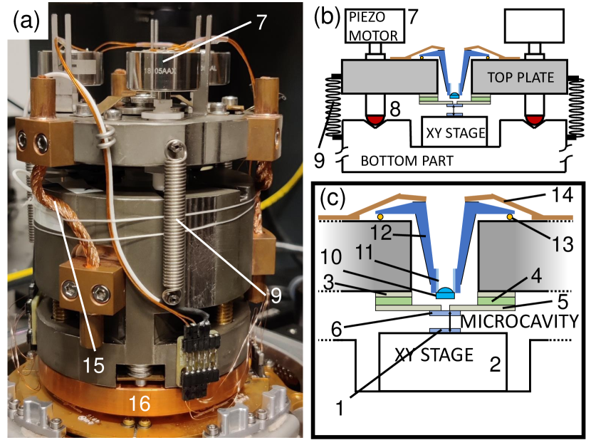
Figure 1: Picture (a) and sketch (b), (c) of the open-cavity device. The top plate and bottom part, as well as the lens mount (11, 12), are made from invar and held together by springs; the bottom part is clamped to the cold base plate of the cryostat by a copper adapter disc (16). Three copper braids are used to cool the top plate (15). The other elements are described in the main text.

As shown in Fig. 1(a) and (b), the device is divided into two parts: the top plate, and the bottom part. The bottom flat mirror (1) is mounted with grease on a custom-built high-stiffness XY translation stage (2) that consists of a polished sapphire plate on top of a XY shear piezo glued to the bottom part of the device, similar to those used in STMs (mashoffLowtemperatureHighResolution2009a, ). The XY stage has a step size in the nanometer range, with a travel range of about 5 mm. The top plate has a hole in its center for optical access. On the bottom side of the top plate, the top cavity mirror mount is attached, in an assembly which consists of a ring-shaped alumina disk (3), a ring piezo (4), another alumina ring-shaped disk (5) and the micro mirrors array (6), all glued together withe epoxy adhesive (EPO-TEK H74F), which is proven to deliver strong and stiff connections in SPM vacuum applications. The thickness of the two alumina disk has been chosen to minimize cavity length changes during cooldown. The ring piezo (4) (Noliac NAC2125) is used for precision scanning and active stabilization of the cavity length. The relative alignment of the two cavity mirrors is accomplished with 3 piezo motors (JPE CLA 2201) in a tip-tilt configuration (7), which enables adjustment of the distance as well as the angles between the top and bottom mirrors with nanometric precision. To ensure mechanical stability and to decouple the movement of the top plate from a XY translation, the 3 ceramic spherical tips (8) at the end of the spindle of the piezo motors are resting in three v-grooves engraved on the upper side of the bottom part. Finally, the top plate and bottom part are held together with three metal springs (9) each exerting a force of 12 N, tuned such that the piezo motors run. Mode matching to the microcavity mode is achieved with an aspheric lens with 0.4 NA (10), mounted in a lens holder consisting of an invar micrometric screw (11) in a threaded invar cone (12) housed in the central hole of the top plate. The lens holder has a smaller diameter than the hole in the top part, in such a way that the lens can be translated in the XY plane for alignment with the optical microcavity mode, and is resting on 3 ruby balls (13) of 1 mm diameter,K glued into holes made in the top invar plate. After aligning the lens in the XY plane and along the z direction (with the micrometric inner screw), it is clamped down with 3 leaf springs (14). To achieve cooling of the top plate, we thermally connected it to the bottom part of the open-cavity device by using 3 copper braids (15): this soft connection minimizes the amount of vibrations transferred to the top plate. The bottom part is clamped to the cold base plate of the cryostat by a copper adapter disk (16), therefore even though this connection acts as a mechanical low-pas filter, there is no additional dedicated mechanical low-pass filter between the cryostat and our device.

The choice of the particular ring piezo mounted on the top plate is a compromise asusually one would choose a small-diameter piezo element with smaller capacitance and therefore higher possible bandwidth, but our choice is limited by the mode matching lens: due to its short working distance (3.39 mm), in order to get close to the concave top cavity mirror, the lens must fit in the hole of the ring piezo, therefore limiting its minimum size. The material of choice for the bottom part, top plate and lens mount, is Invar-36 which has been proven a good solution in designing optical cryogenic systems, due to its low thermal expansion coefficient (fedoseevRealignmentfreeCryogenicMacroscopic2022, ). The small integrated (300 K $\rightarrow$ 4 K) expansion coefficient results in a small focal shift of the lens, and ensures minimal optical realignment after cool-down.

The use of nanopositioners and piezo elements is crucial for the alignment and operation of the microcavity, but the complex structure of these actuators introduces mechanical resonance frequencies of the device. In particular the lowest-frequency mechanical resonance of the cavity device that significantly affects the cavity length reduces the passive mechanical stability (chenIntroductionScanningTunneling2007, ) and the maximum possible bandwidth of the feedback stabilization circuit (bechhoeferFeedbackPhysicistsTutorial2005, ). In order to push this mechanical resonance as high as possible in frequency, we maximized the stiffness of the open-cavity device by connecting the different parts together by using either springs with high spring constants or a high-performance epoxy adhesive. Additionally we preserved as much as possible a rotational symmetry with respect to the central axis of the open-cavity device: this avoids mechanical mode-splitting and reduces the number of mechanical resonances in the device.

II Device characterization: feedback loop and mechanical resonances

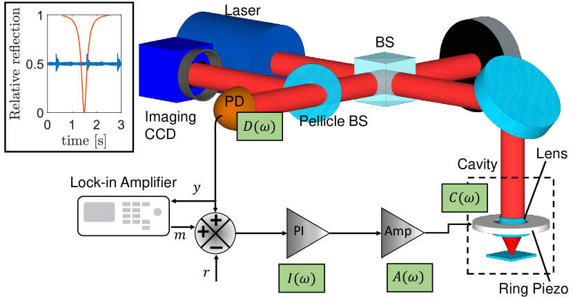
Figure 2: Optical scheme for measuring the open-loop transfer function of the feedback loop: laser light is coupled to the cavity, and the backreflection is both monitored with an imaging CCD and measured by a photodiode, giving a signal $y$. The difference between $y$ and a reference signal $r$ is the error signal that is fed into a PI controller that controls the ring piezo via an amplifier. A lock-in amplifier is used to measure the signal $y$ from the photodiode and to add a modulation $m$ on top of it, in order to measure the open loop transfer function of the feedback. The inset shows the cavity reflection dip as well as a time trace of the stabilized cavity length.

We now introduce the experimental setup that we will use in the rest of this paper, we discuss the negative feedback circuit used for active stabilization of the cavity length and we show how measuring the transfer function of this feedback loop we can characterize the resonances of the open-cavity device (reinhardtSimpleDelaylimitedSideband2017, ; janitzHighMechanicalBandwidth2017, ; saavedraTunableFiberFabryPerot2021, ). This knowledge is of extreme importance not only because the lowest mechanical resonance present in the device can pose a serious limitation on the active stabilization, but also because it limits the passive stability as discussed in (chenIntroductionScanningTunneling2007, ). The identification of the mechanical resonances helped us improving the stability of the open-cavity device, by redesigning some of its parts iteratively.

II.1 Optical setup:

We operate the microcavity in reflection, as shown in Fig. 2: a collimated laser beam is sent to the mode-matching lens of the open-cavity device which couples light to the cavity, the reflected light travels back along the same path, and is redirected to a photodiode (Thorlabs PDA-36 EC) by a beam splitter. Before reaching the photodiode, part of the light is also sent to an imaging CCD by a pellicle beam splitter, allowing imaging of the micromirrors array, and also observation of the shape of the particular transverse mode excited in the cavity. We use narrow-linewidth tunable diode lasers in a range from $\lambda=\>935$ nm to 1000 nm. The Bragg coating of our cavity micro-mirrors is centered at $\lambda=\>935$ nm for which the cavity has a Finesse $F\sim$ 2500. The maximum coupling efficiency we obtained at $\lambda=\>935$ nm is $\eta=$ 64%, and we reach $\eta=$ 80% at a different wavelength where the cavity has a finesse $F$ = 500. We have identified scattering losses of the mirrors as the main limiting factor for the coupling efficiency. The cavity resonance reflection dip is shown in the inset of Fig. 2.

II.2 Cavity stabilization feedback loop

In order to keep the cavity resonant with the laser, we use active stabilization of the cavity length: the signal from the photodiode is sent through a lockbox (PI controller with scanning and locking capabilities), then a low noise piezo amplifier (Falco Systems WMA-200) that drives the ring piezo. Each of these stages has a specific frequency dependent and complex transfer function, defined as the ratio between the output and input voltages of that stage. Here and in the following we will use interchangeably the words $`$gain’ and ‘transfer function’. We define the transfer functions of the PI controller as $I(\omega)$, the piezo amplifier $A(\omega)$, the optical micro-cavity $C(\omega)$, and the photodiode $D(\omega)$. The product of these quantities $G(\omega)=\>IACD$ is the open loop gain of the feedback loop, i.e., the ratio between the voltage measured on the photodiode and the voltage entering the PI controller, when the output of the photodiode is disconnected from the PI controller, i.e., when the feedback loop is open.

We now quantify the contribution of each individual stage, in order to provide insight into the overall gain $G$. $I$ is the gain of the PI controller, and it is given by $I(\omega)=1/(j\omega\tau_{I})+G_{P}$, where the frequency dependent part is given by the integrator, and the constant part is given by the proportional term. $\tau_{I}$ is the integration time, and inversely proportional to the integral gain. The piezo amplifier has a gain $A(\omega)=A_{0}/(1+j\omega/\omega_{c})$ , where $\omega_{c}=\>2\pi f_{C}$. In our case $A_{0}=\>20,$ and the cutoff frequency is $f_{c}=$ 4600 Hz when the amplifier is driving the ring piezo which has a capacitance of 700 nF. The gain of the cavity C($\omega)$ and the photodiode D($\omega)$ are a bit more complicated to express, as they involve a conversion from the input Voltage to different physical quantities. First the input voltage is applied to the piezo, which in turn gives a displacement based on the piezoelectric coefficient $r_{piezo}\>[\textrm{nm}/\textrm{V}]$, then the displacement of the piezo changes the cavity length, which in turn changes the amount of light power that is reflected back and sent to the photodiode, as shown in the inset of Fig. 2. The power is then converted into a voltage signal by the photodiode. Since we will lock the cavity at half of the reflection dip (side-of-fringe lock), which gives maximum sensitivity to changes of the cavity length, we will give the overall gain of the cavity and photodiode together: $CD$($\omega)=-r_{piezo}\times 2\eta V_{0}F/\lambda$, where $\eta$ is the coupling efficiency of the light to the cavity, $F$ is the finesse, $\lambda$ is the wavelength of the incident light and $V_{0}$ is the voltage on the photodiode when the cavity is tuned off-resonance. This gain is different for different measurements, since we vary the cavity finesse by adjusting the laser wavelength, which also changes the laser power and with this $V_{0}$. Moreover the piezoelectric coefficient is $r_{piezo}=3.8\textrm{ {nm}/{V}}$ at room temperature, but becomes a factor $\sim$ 3 lower when operating the cavity at 4 K. As an example, at room temperature we have $CD$ = 7.1 with $\lambda=\;935$ nm, $F$ = 2500 and a typical value of $V_{0}=0.7$ V and $\eta=\>0.5$.

II.3 Identification of mechanical resonances

Up to now $CD$ is frequency independent, but we will now show that this is not true, and how its frequency dependency can be used to find the mechanical resonances of the open cavity device. The ring piezo is mechanically coupled to the rest of the open cavity device, and therefore to all its mechanical resonances. Because of this, the piezoelectric coefficient $r_{piezo}$ is in fact frequency dependent, and will show a resonance–anti-resonance behavior in proximity of the mechanical resonances present in the system (ryouActiveCancellationAcoustical2017, ). This shows up in the total open loop transfer function of the feedback loop as shown in Fig. 3. This measurement has been done with a locked cavity, using a lock-in amplifier to apply a frequency-swept small modulation $m$ to the input port of the PI controller and to measure the signal from the photodiode $y$, from which the open-loop gain $G$ is calculated as:

$$G(\omega)=\frac{H(\omega)}{1+H(\omega)},\!\textrm{with }H(\omega)=\frac{y(\omega)}{m}$$ (2)

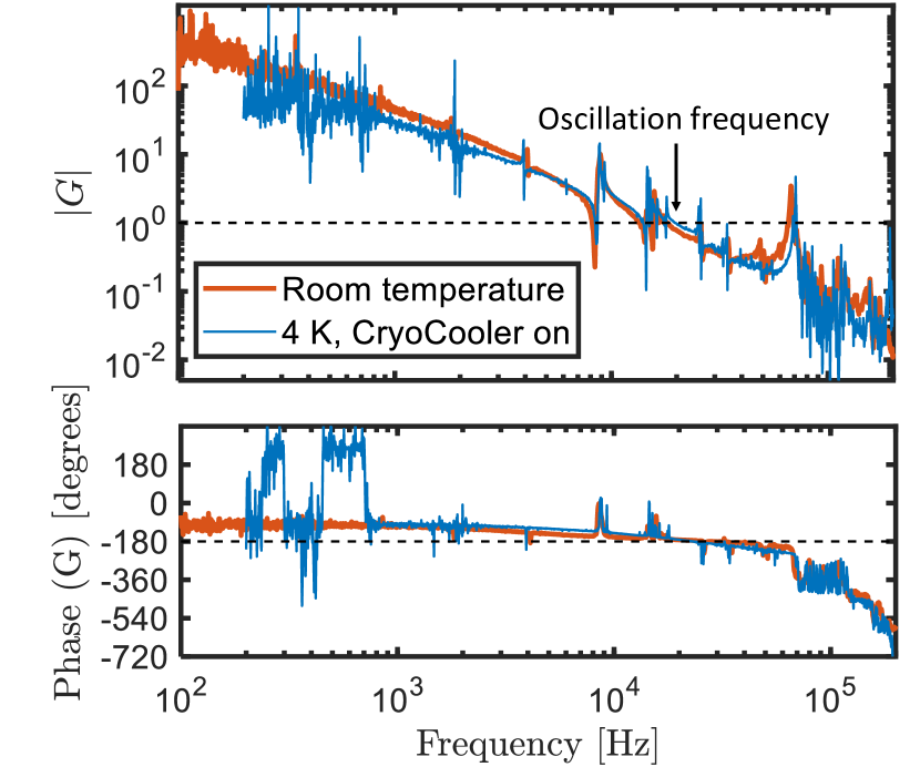
Figure 3: Measured amplitude and phase (unwrapped) of the feedback loop transfer function for two different conditions: device mounted in the cryostat with the cryocooler switched off at room temperature and ambient pressure (red), and at 4 K with the cryocooler on (blue). The positions of the mechanical resonances is not significantly shifted at low temperature. The dashed lines corresponds to unity gain and -$\pi$ phase respectively; the feedback loop oscillates at 22.8 kHz if the gain is set too high.

By performing several measurements of the transfer function $G$ while damping, removing or changing the configuration of specific parts of the open-cavity device, we were able to identify the origin of several mechanical resonances, and to redesign the responsible components in order to remove or shift them to higher frequencies. After device optimization, we obtain the transfer function $G$ shown in Fig. 3 of the device mounted in the cryostat at room temperature (red curve) and at 4 K with the cryocooler on (blue curve). The cryocooler leads to noise, particularly visible at low frequencies. We observe only a small shift and change of the resonance frequencies while cooling down. At 4 K the first -$\pi$ phase crossing happens at 4.1 kHz and the first unity gain frequency is at 8.58 kHz, while the feedback loop oscillation frequency is 22.8 kHz. For a simple system with only one mechanical resonance these 3 frequencies would coincide, but our open-cavity device is more complex as there are many mechanical resonances coupled with the resonance of the ring piezo. We identified some of the resonances to be drum modes of the top plate (8.58 kHz, 14.3 KHz, 15.6 kHz, 26 kHz and 35 kHz). We were not able to pinpoint the origin of the resonances at 1.8 kHz, 2 kHz and 4.1 kHz.

III Stability at room temperature

To measure the stability of the cavity, we use the scheme shown in Fig. 2 but without the modulation signal $m$, and again locking the cavity to the laser frequency using a side-of-fringe lock. In particular, we lock the cavity at half the depth of the reflection dip, and we record 10 time traces of 10 s of the photodiode signal at a sample rate of 200 kHz. After a proper calibration (see Appendix B) we calculate the power spectral density (PSD) of these time traces, corresponding to fluctuations in the cavity length. In Fig. 4 we show data measured (i) on the optical table resting on air dampers, (ii) in the cryostat under vacuum, (iii) in the cryostat under vacuum with the cryocooler switched on but still at room temperature, (iv) same conditions as iii but only considering the quiet periods of the cryocooler, corresponding to 40% of the full period. Panel (a) shows an exemplary section of the time traces, and (b) shows the corresponding PSDs. The finesse of the cavity is 1500, and the PI parameters are $\tau_{I}$ = 30 $\mu s$, $G_{P}$ = 0.17.

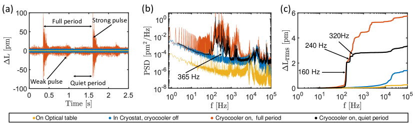
Figure 4: Room-temperature stability measurements of the open-cavity device for 3 different conditions: mounted on the optical table (yellow), mounted in the cryostat under vacuum (blue), and in the cryostat under vacuum and with the cryocooler switched on (red). Note that the measurement in yellow corresponds to an earlier version of the cavity device. (a) Time trace of the signal from the photodiode, for a cavity locked at half of the reflection dip. (b) Power spectral density of the signal from the time traces. (c) Cumulative cavity length fluctuation as a function of frequency. The cavity finesse is $F=1500$ in all cases.

Comparing the measurements without cryocooler, it is clear that the cavity length is more stable when the device is mounted directly on the optical table (yellow trace), than when it is mounted in the cryostat. The rms cavity length fluctuations integrated from 1 Hz to 100 kHz are $\Delta L_{rms}=0.29$ pm on the optical table, and $\Delta L_{rms}=1.5$ pm mounted in the cryostat. This decrease in stability can be attributed to mechanical noise entering the cavity through the connections of the cryostat to the rest of the lab environment (such as the high-pressure helium flex lines): this noise bypasses the low-pass filter of the optical table. The small peak at 365 Hz in the PSD (blue) of Fig. 4(b) corresponds to a mechanical resonance in the base of the cryostat.

Focusing on the measurement with the cryocooler switched on, the time traces show a stronger and a weaker pulse, both with period 1.25 s (0.8 Hz) separated by 0.625 s. In the PSD we can see harmonics of this frequency up to kHz frequencies. By calculating the PSD for different bandwidths, we can plot the cumulative cavity length fluctuation in Fig. 4(c), this enables best understanding of the frequencies that contribute most to the mechanical noise.

Because of the large cavity length changes caused by the spikes of the cryocooler, here and in the rest of the paper we define a quiet period in between the small spike and the big spike, corresponding to 40% of the time between 2 large spikes, and we will use it to calculate the PSD and noise characteristics of the cavity device. In this way the PSD will also be cleaner as all the cryocooler harmonics caused by the train of pulses in the time trace will be removed, and it will be easier to identify mechanical resonances. The PSD and the cumulative rms noise are shown as black lines in Fig. 4(b) and (c). During the quiet period we obtain an rms cavity length fluctuation of $\Delta L_{mrs}=3.4$ pm, as opposed to 5.7 pm if measured over the full period of the cryocooler. As can be seen from the cumulative cavity length fluctuations, the major contribution to the mechanical noise comes from frequencies lower than one kHz, in particular 160 Hz, 240 Hz, 320 Hz. These frequencies are not resonances of the cavity device, as they are not visible in the transfer function measurement shown in Fig. 3, and they appear in the cryostat measurements only when the cryocooler is switched on. Further evidence of this is presented in Appendix A.

IV Stability in a closed-cycle cryostat at 4 K

Now we describe the cool-down, re-alignment and measurements under cryogenic conditions. With the aid of a copper adapter plate, the open-cavity device is tightly mounted on the base of the closed-cycle cryostat. The cavity is aligned at room temperature using the nanopositioners and the external optics, before the system is cooled down to 4 K. By monitoring the free spectral range of the cavity during cool-down, we observe a change in the cavity length of $\Delta L=5.5$ µm. Once at 4 K, the cavity length can be readjusted with the 3 piezo motors if needed. We control the finesse of the cavity by detuning the laser frequency, which changes the mirror reflectivity, such that we obtain the highest finesse cavity that can be locked despite the noise from the cryocooler. The PI parameters of the feedback system are well-controlled as described in section II. In practice, the highest possible finesse is obtained when the peak-to-peak displacement of the cavity length caused by the cryocooler is slightly smaller than the FWHM of the reflection cavity resonance dip, beyond that the lock is lost during every cryocooler cycle. We usually start with a laser frequency far detuned from the thin-film mirror stop-band center, locking the cavity and optimizing the PI parameters to minimize the mechanical noise in the cavity length, then slightly changing the laser frequency in order to increase the finesse of the cavity, and iterating the procedure until the PI controller is not able to keep the cavity locked.

The thin-film mirror design wavelength is 935 nm, resulting in a cavity finesse of 2500. In our case the highest finesse we were able to achieve is 1800 at $\lambda$ = 990 nm, for which we have a stable lock that lasts for at least 2 days without any adjustment, by using the PI parameters $\tau_{I}$ = 50 $\mu s$ and $G_{P}$ = $0.03$. As described in the previous section, once the cavity is locked at half of the reflection dip, we record 10 time traces each 10 s long of the photodiode signal. After converting this voltage signal into cavity length fluctuations (see Appendix B), we calculate the PSD and the cumulative integrated rms noise to identify the frequencies that contribute most strongly.

In Fig. 5(a) we show a reflection dip and a small portion of the calibrated time trace taken with a locked cavity, that represents the fluctuations of the cavity length from the locked position. The red vertical line corresponds to the maximum peak cavity length fluctuation that allows locking of the cavity, while the red-highlighted part of the time trace corresponds to the quiet period of the cryocooler (40% of the full period). Using the calibrated time trace, we calculate the power spectral density and the cumulative cavity length fluctuation for the quiet period (red) and for the full period (blue) of the cryocooler, as shown in Fig. 5(b). The total rms mechanical noise in a 100 kHz bandwidth is 5.7 pm during the quiet period of the cryocooler and 10.6 pm during the full period. As it is clearly visible in the plot, also at 4 K, the major contribution to the noise comes from the same low frequencies that were present at room temperature with operating cryocooler, in particular at 160 Hz and 240 Hz. In addition, now there is also mechanical noise at 400 Hz, which we think is a mechanical resonance of the base of the cryostat that shifted from the room temperature value of 365 Hz. Only a small part of the noise comes from resonances of the open-cavity device itself, one small contribution at 1.9 kHz (compare Fig. 3), and a contribution from 22.8 kHz, which is the oscillation frequency of the feedback loop. We note that the contribution from 22.8 kHz is significant only in the full period curve (blue), because the pulses from the cryocooler bring the feedback close to instability.

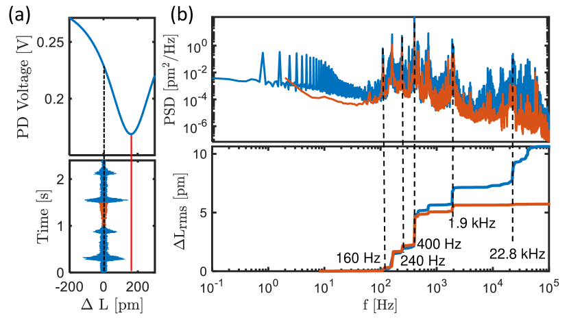
Figure 5: Stability measurement at 4 K for a cavity finesse $F$ = 1800 ($\lambda=990$ nm). Panel (a) shows the calibration curve and a section of a time trace of the cavity length displacement. The red-highlighted part in (a) corresponds to the quiet period of the cryocooler. In (b) are shown the PSD and cumulative noise corresponding to the quiet period (red) and full period (blue) of the cryocooler. The rms mechanical noise is 5.7 pm in the quiet period, ad 10.6 pm in the full period.

V Conclusions and outlook

In conclusions, we have developed an open-access optical microcavity compatible with a tabletop optical closed-cycle cryostat. At 4 K, the open cavity device has stabilities of 5.7 and 10.6 pm rms during the quiet and full period of the cryocooler cycle, respectively. The device allows for full nanometric but millimiter-range tunability of the cavity along the three spatial directions and two angles, and minimal optical realignment when cooling down to 4 K. The key to this is an extremely high-stiffness and compact design, which allows using active feedback stabilization of the cavity with a very high bandwidth.

Most importantly, our design does not use a dedicated mechanical low pass filter, which would complicate integration of the cavity in a free-space optical setup, essential for instance for full polarization control. Nevertheless a low-pass filter would increase the stability of our open-access optical microcavity. We estimate that a combination of a mechanical low pass filter at around 50 Hz and electronic filtering in the feedback loop (ryouActiveCancellationAcoustical2017, ; okadaExtendingPiezoelectricTransducer2020, ), will allow us to achieve at cryogenic temperatures the same cavity stability as on an optical table at room temperature.

VI Aknowledgements

We would like to thank G. Verdoes and E. Wiegers for helping with the construction of the open-cavity device, and K. Heeck for useful discussions on the electronics part. We acknowledge funding from a NWO Vrij Programma Grant (QUAKE, 680.92.18.04), the European Union’s Horizon 2020 research and innovation programme under grant agreement No. 862035 (QLUSTER), and the Quantum Software Consortium.

Appendix A Comparison of cryocooler in low- and high-power mode

The Gifford-McMahon Cryocooler used in our cryostat can be operated in a low-power (LP) and high-power (HP) mode. We compare here the effects of the two different settings on the stability of the open-cavity device. As a result of the exchange Helium gas undergoing compression-expansion cycles, the cryocooler introduces mechanical noise in the open-cavity device, in the form of pulses. The frequency of this cycle is 0.8 Hz for LP and 1.01 Hz for HP mode, corresponding to the frequency at which the compressed gas enters the regenerator through the high-pressure line. In the middle of the cycle, the Helium gas expands and returns to the compressor. This results in two mechanical pulses per cycle of the base plate of the cryostat.

In Fig. A1(a) and (b) we show the fluctuation of the cavity length measured over time with the cryocooler in the LP and HP mode, where the cavity length is actively stabilized by locking at half of the reflection dip as explained in the main text. Each plot shows two kinds of pulses corresponding to the high and low pressure part of the cycle. Comparing Fig. A1(b) to Fig. A1(a) we see that in addition to the higher frequency of the pulses, the peak-to-peak amplitude of the pulse is also higher, as a result of the increased pressure difference of the Helium.

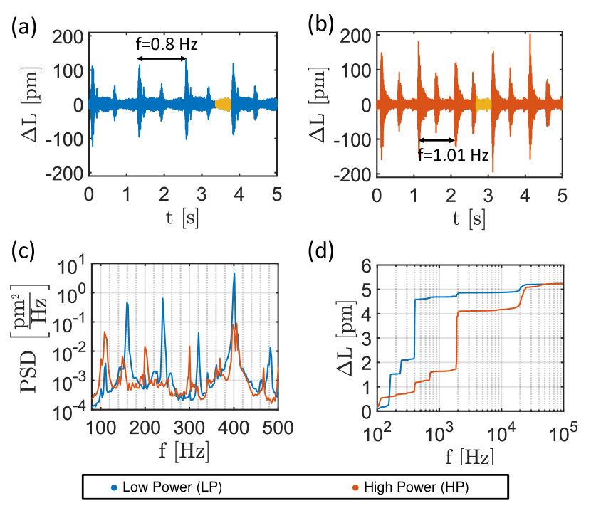
Figure A1: Comparison of low- and high-power mode. Panels (a) and (b) show the measured cavity length fluctuations as a function of time for LP (a) and HP (b) mode. The yellow portion of the data is used to calculate the PSD shown in (c) and the cummulative length fluctuations (d), blue curves for LP and red curves for HP mode.

We calculated the power spectral density (PSD) as explained in the main text, by considering the yellow sections of the time traces in Fig. A1(a) and (b) which corresponds to the quiet period, i.e. 40% of the cycle for the high power setting. We considered the same section also for the low power mode, so that the frequency separation of the points in the PSD is the same for both configurations, making a comparison easier. As explained in the main text, we take 10 time traces of 10 seconds each, for each time trace we select the orange sections in each cycle of the cryocooler, we calculate the PSD of each section and finally we average them together. The result of this process is shown in Fig. A1(c), where we plot only a small frequency range 80-500 Hz because outside of this range, there are not many differences between LP and HP mode, except for the peak heights. In particular, in both PSDs we see a 400 Hz peak corresponding to a resonance of the base of the cryostat as motivated in the main text. All other low frequency peaks that are visible in the LP mode (160 Hz, 240 Hz and 320 Hz), are not present in HP mode, where there are now three extra peaks at 150 Hz, 200 Hz and 300 Hz, most likely harmonics of 50 Hz line noise.

Despite we do not know the exact origin of the peaks at 160 Hz, 240 Hz and 320 Hz, we can conclude that it is noise introduced by the cryocooler and these peaks do not correspond to mechanical resonances in the system because otherwise they should be visible also with the cryocooler in HP mode. Because of the constant frequency separation between these peaks, one hypothesis is that they originate from the inverter used in the He compressor, as in LP mode the frequency of the inverter is 40 Hz.

Fig. A1(d) shows the cumulative cavity length fluctuation measured in the quiet period of the cryocooler cycle. The total rms noise $\Delta L_{rms}$ = 5.3 pm is nearly the same for the two modi, despite the frequencies that contribute to the noise are different. We have used the same PI parameters for both measurements, optimized for the LP mode for minimum vibrations. The feedback loop is less stable in the HP mode due to a higher peak-to-peak amplitude of the pulses excited by the cryocooler, as visible in the 22.8 kHz peak corresponding to the oscillation frequency of the feedback loop.

Appendix B Calibration of the Photodiode signal

In order to measure the stability of the cavity device, we lock the cavity length to half of the reflection dip and we record time traces of the voltage signal from the photodiode, as explained in the main text. This voltage must be multiplied by a conversion factor in order to give a measure of the cavity length. While this is trivial in the case of a quiet system where the cavity length does not change much and therefore this conversion factor is simply the slope of the reflection dip at the locking point, in the case of a mechanically noisy system, it is more complicated. In fact, when the cavity length changes significantly, the error signal can not be approximated anymore as being linear, and in order to retrieve the exact cavity length, we must take the nonlinearities into account. For this purpose we calibrate the voltage signal of the photodiode $V_{PD}$ as a function of the cavity length $L$, by linearly changing the latter via the ring piezo and recording the reflection dip, which is fitted with a Lorentzian

$$V_{PD}=V_{0}+\frac{A}{(L-L_{0})^{2}+(\frac{w}{2})^{2}}\ .$$ (A1)

Inverting the equation, we are able to obtain a conversion factor from photodiode voltage to cavity length :

$$L=L_{0}\pm\sqrt{\frac{A}{V_{PD}-V_{0}}-\left(\frac{w}{2}\right)^{2}}$$ (A2)

where the $\pm$ sign is chosen depending wheter the cavity is locked on the left or right side of the reflection dip. $A$, $V_{0},$ $L_{0}$ and $w$ are fitting parameters, $w$ is the full width at half maximum of the reflection dip, and $L_{0}$ is the resonance cavity length, for which the reflection dip has its minimum.

While this procedure takes into account the nonlinearity of the error function, it still has some drawbacks: for the calibration we scan the cavity length at a finite speed, and in presence of vibrations, the shape of the reflection dip will change depending on the speed at which the cavity is scanned, leading to shifts in the position of the dip, broadening of the cavity reflection dip and asymmetries. In Fig. A2(a) we demonstrate this effect. We have recorded four times a cavity dip, and we observe four very different results, with extracted finesses varying from 1100 to 4600. The real room-temperature finesse is measured to be F = 2500 at a wavelength $\lambda$ = 935 nm. A simple way to deal with this is to measure the width of the reflection dip at room temperature without mechanical vibrations as a function of the wavelength of the laser, and use this value to obtain the conversion factor of Eq. A2, as we expect the reflectivity of the mirrors to be constant from 300 K to 4 K.

As an additional proof and to have a better understanding of the phenomena, we show here measurements of the shifts of the resonance widths and dips ($w$, $L_{0}$) and compare it to simulations.

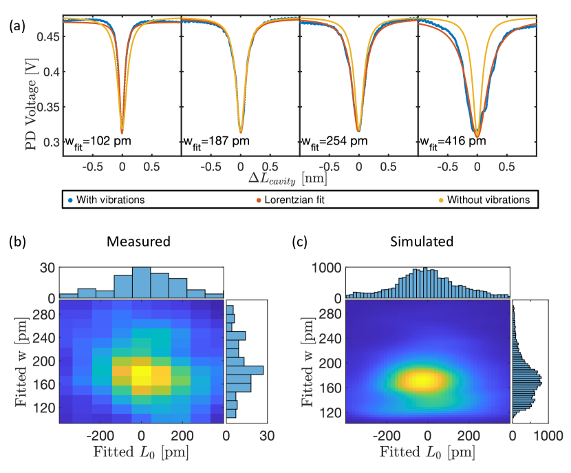
Figure A2: (a) In blue four measurements of a cavity resonance recorded at 4 K with cryocooler ON, with the same scanning speed but at different times of the cryocooler cycle . In red the corresponding Lorentzian fit, and in orange the real cavity resonance measured at room temperature without vibrations. (b) Scatter plot and relative histograms of the fitted widths and positions of the cavity resonance, measured at 4 K. (c) Scatter plot and relative histograms of the fitted widths and positions of the cavity resonance, result of a computer simulation.

For the measurement we recorded 150 reflection dips at 4 K with the mechanical noise generated by the cryocooler, by scanning repeatedly the cavity length with the ring piezo. We fit each reflection dip using Eq. A1, and we show the resulting scatter plot in Fig. A2(b). The data of the scatter plot have been convoluted with a Gaussian mask function with witdth of 10 pm, to smooth the data due to the low number of samples. The mean value for the width is $w_{mean}=189$ pm, in very good agreement with the real value of 185 pm. The mean value for $L_{0}$ is around 0 as we shifted the data manually, since we do not know the real position of the resonance in absence of vibrations. For the simulation, we used the power reflection coefficient of a Fabry-Perot cavity:

$$R(L)=\left|\frac{E_{reflected}}{E_{incident}}\right|^{2}=\left|\frac{r\left(\exp\left(i\frac{4\pi L}{\lambda}\right)-1\right)}{1-r^{2}\exp\left(i\frac{4\pi L}{\lambda}\right)}\right|^{2}$$ (A3)

where $L=L_{piezo}+L_{noise}$. $L_{piezo}=v_{piezo}\times t$, and $v_{piezo}$ is the scanning speed of the piezo. For $L_{noise}$ we used the measured displacements from Fig. A1 (a), recorded with a cavity locked on the side of the reflection dip, where we compensated for the effect of the integrator: $L_{noise}=(1+I)\times L_{noise}^{lock}$. We chose a mirror reflectivity R = $r^{2}$ = 0.988 which correspond to a cavity with Finesse F $\sim 2600$, and a resonance width of $w$ = 178 pm at the wavelength $\lambda$ = 935 nm. For all other free parameters such as $v_{piezo}$ and the open loop gain of the integrator $I$, we have used experimental values.

We have simulated 20000 reflection dips using Eq. A3 by randomly shifting in time the experimental $L_{noise}$, and we fitted the curves with Eq. A1 in order to extract $w_{fit}$ and $L_{0}^{fit}$. The results are shown in Fig. A2(c), where the data have been smoothed by convolution with a Gaussian mask function. The mean values are $w_{mean}=179$ pm and $L_{0}^{mean}=-1.7$ pm. Visually the distribution in Fig. A2(c) is clearly shifted towards negative $L_{0}$, we hypothesize that this is because of the forces that keep together the two mirrors, i.e. gravity and the three metal springs holding together the top plate and the bottom part of the open cavity device. Since $L_{0}$ is the rest-length of the cavity, mechanical vibrations in the open-cavity device will exert sinusoidal forces that act on the same direction of gravity and the spring force for $L_{0}<0$, and in the opposite direction for $L_{0}>0$, causing the asymmetry visible in the histogram. The very good agreement between the measured data and the simulation, as well as the comparison to the reflection widths measured in absence of noise, shows us that indeed we can calibrate the photodiode signal at 4 K with the value of width measured at room temperature for the same wavelength.

References

- (1) Vahala, K. J. Optical Microcavities. Nature 424, 839 (2003).
- (2) Ding, X., He, Y., Duan, Z.-C., Gregersen, N., Chen, M.-C., Unsleber, S., Maier, S., Schneider, C., Kamp, M., Höfling, S., Lu, C.-Y. & Pan, J.-W. On-Demand Single Photons with High Extraction Efficiency and Near-Unity Indistinguishability from a Resonantly Driven Quantum Dot in a Micropillar. Physical Review Letters 116, 020401 (2016).
- (3) Somaschi, N., Giesz, V., De Santis, L., Loredo, J. C., Almeida, M. P., Hornecker, G., Portalupi, S. L., Grange, T., Antón, C., Demory, J., Gómez, C., Sagnes, I., Lanzillotti-Kimura, N. D., Lemaítre, A., Auffeves, A., White, A. G., Lanco, L. & Senellart, P. Near-Optimal Single-Photon Sources in the Solid State. Nature Photonics 10, 340 (2016).
- (4) Tomm, N., Javadi, A., Antoniadis, N. O., Najer, D., Löbl, M. C., Korsch, A. R., Schott, R., Valentin, S. R., Wieck, A. D., Ludwig, A. & Warburton, R. J. A Bright and Fast Source of Coherent Single Photons. Nature Nanotechnology 16, 399 (2021).
- (5) Thomas, S. E., Billard, M., Coste, N., Wein, S. C., Priya, Ollivier, H., Krebs, O., Tazaïrt, L., Harouri, A., Lemaitre, A., Sagnes, I., Anton, C., Lanco, L., Somaschi, N., Loredo, J. C. & Senellart, P. Bright Polarized Single-Photon Source Based on a Linear Dipole. Physical Review Letters 126, 233601 (2021).
- (6) Snijders, H., Frey, J. A., Norman, J., Post, V. P., Gossard, A. C., Bowers, J. E., van Exter, M. P., Löffler, W. & Bouwmeester, D. Fiber-Coupled Cavity-QED Source of Identical Single Photons. Physical Review Applied 9, 031002 (2018).
- (7) Evans, R. E., Bhaskar, M. K., Sukachev, D. D., Nguyen, C. T., Sipahigil, A., Burek, M. J., Machielse, B., Zhang, G. H., Zibrov, A. S., Bielejec, E., Park, H., Lončar, M. & Lukin, M. D. Photon-Mediated Interactions between Quantum Emitters in a Diamond Nanocavity. Science 362, 662 (2018).
- (8) Kimble, H. J. The Quantum Internet. Nature 453, 1023 (2008).
- (9) Cirac, J. I., Zoller, P., Kimble, H. J. & Mabuchi, H. Quantum State Transfer and Entanglement Distribution among Distant Nodes in a Quantum Network. Physical Review Letters 78, 3221 (1997).
- (10) Northup, T. E. & Blatt, R. Quantum Information Transfer Using Photons. Nature Photonics 8, 356 (2014).
- (11) Bonato, C., Haupt, F., Oemrawsingh, S. S. R., Gudat, J., Ding, D., van Exter, M. P. & Bouwmeester, D. CNOT and Bell-state Analysis in the Weak-Coupling Cavity QED Regime. Physical Review Letters 104, 160503 (2010).
- (12) Hacker, B., Welte, S., Rempe, G. & Ritter, S. A Photon–Photon Quantum Gate Based on a Single Atom in an Optical Resonator. Nature 536, 193 (2016).
- (13) Trupke, M., Hinds, E. A., Eriksson, S., Curtis, E. A., Moktadir, Z., Kukharenka, E. & Kraft, M. Microfabricated High-Finesse Optical Cavity with Open Access and Small Volume. Applied Physics Letters 87, 211106 (2005).
- (14) Barbour, R. J., Dalgarno, P. A., Curran, A., Nowak, K. M., Baker, H. J., Hall, D. R., Stoltz, N. G., Petroff, P. M. & Warburton, R. J. A Tunable Microcavity. Journal of Applied Physics 110, 053107 (2011).
- (15) Greuter, L., Starosielec, S., Najer, D., Ludwig, A., Duempelmann, L., Rohner, D. & Warburton, R. J. A Small Mode Volume Tunable Microcavity: Development and Characterization. Applied Physics Letters 105, 121105 (2014). eprint 1408.1357.
- (16) Wachter, G., Kuhn, S., Minniberger, S., Salter, C., Asenbaum, P., Millen, J., Schneider, M., Schalko, J., Schmid, U., Felgner, A., Hüser, D., Arndt, M. & Trupke, M. Silicon Microcavity Arrays with Open Access and a Finesse of Half a Million. Light: Science & Applications 8, 37 (2019).
- (17) Najer, D., Söllner, I., Sekatski, P., Dolique, V., Löbl, M. C., Riedel, D., Schott, R., Starosielec, S., Valentin, S. R., Wieck, A. D., Sangouard, N., Ludwig, A. & Warburton, R. J. A Gated Quantum Dot Strongly Coupled to an Optical Microcavity. Nature 575, 622 (2019).
- (18) Koks, C., Baalbergen, F. B. & van Exter, M. P. Observation of Microcavity Fine Structure. Physical Review A 105, 063502 (2022).
- (19) Mader, M., Reichel, J., Hänsch, T. W. & Hunger, D. A Scanning Cavity Microscope. Nature Communications 6, 7249 (2015).
- (20) Bogdanović, S., van Dam, S. B., Bonato, C., Coenen, L. C., Zwerver, A.-M. J., Hensen, B., Liddy, M. S. Z., Fink, T., Reiserer, A., Lončar, M. & Hanson, R. Design and Low-Temperature Characterization of a Tunable Microcavity for Diamond-Based Quantum Networks. Applied Physics Letters 110, 171103 (2017).
- (21) Vadia, S., Scherzer, J., Thierschmann, H., Schäfermeier, C., Dal Savio, C., Taniguchi, T., Watanabe, K., Hunger, D., Karraï, K. & Högele, A. Open-Cavity in Closed-Cycle Cryostat as a Quantum Optics Platform. PRX Quantum 2, 040318 (2021).
- (22) Fontana, Y., Zifkin, R., Janitz, E., Rodríguez Rosenblueth, C. D. & Childress, L. A Mechanically Stable and Tunable Cryogenic Fabry–Pérot Microcavity. Review of Scientific Instruments 92, 053906 (2021).
- (23) Pallmann, M., Eichhorn, T., Benedikter, J., Casabone, B., Hümmer, T. & Hunger, D. A Highly Stable and Fully Tunable Open Microcavity Platform at Cryogenic Temperatures. APL Photonics 8, 046107 (2023).
- (24) Hackley, J. D., Kislitsyn, D. A., Beaman, D. K., Ulrich, S. & Nazin, G. V. High-Stability Cryogenic Scanning Tunneling Microscope Based on a Closed-Cycle Cryostat. Review of Scientific Instruments 85, 103704 (2014).
- (25) Battisti, I., Verdoes, G., van Oosten, K., Bastiaans, K. M. & Allan, M. P. Definition of Design Guidelines, Construction, and Performance of an Ultra-Stable Scanning Tunneling Microscope for Spectroscopic Imaging. Review of Scientific Instruments 89, 123705 (2018).
- (26) Chen, C. J. Introduction to Scanning Tunneling Microscopy: Second Edition. Monographs on the Physics and Chemistry of Materials (Oxford University Press, Oxford, 2007).
- (27) Mashoff, T., Pratzer, M. & Morgenstern, M. A Low-Temperature High Resolution Scanning Tunneling Microscope with a Three-Dimensional Magnetic Vector Field Operating in Ultrahigh Vacuum. Review of Scientific Instruments 80, 053702 (2009).
- (28) Fedoseev, V., Fisicaro, M., van der Meer, H., Löffler, W. & Bouwmeester, D. Realignment-Free Cryogenic Macroscopic Optical Cavity Coupled to an Optical Fiber. Review of Scientific Instruments 93, 013103 (2022).
- (29) Bechhoefer, J. Feedback for Physicists: A Tutorial Essay on Control. Reviews of Modern Physics 77, 783 (2005).
- (30) Reinhardt, C., Müller, T. & Sankey, J. C. Simple Delay-Limited Sideband Locking with Heterodyne Readout. Optics Express 25, 1582 (2017).
- (31) Janitz, E., Ruf, M., Fontana, Y., Sankey, J. & Childress, L. High Mechanical Bandwidth Fiber-Coupled Fabry-Perot Cavity. Optics Express 25, 20932 (2017).
- (32) Saavedra, C., Pandey, D., Alt, W., Pfeifer, H. & Meschede, D. Tunable Fiber Fabry-Perot Cavities with High Passive Stability. Optics Express 29, 974 (2021).
- (33) Ryou, A. & Simon, J. Active Cancellation of Acoustical Resonances with an FPGA FIR Filter. Review of Scientific Instruments 88, 013101 (2017).
- (34) Okada, M., Serikawa, T., Dannatt, J., Kobayashi, M., Sakaguchi, A., Petersen, I. & Furusawa, A. Extending the Piezoelectric Transducer Bandwidth of an Optical Interferometer by Suppressing Resonance Using a High Dimensional IIR Filter Implemented on an FPGA. Review of Scientific Instruments 91, 055102 (2020).