Deconfinement Phase Transition in Bosonic BMN Model at General Coupling

Abstract

We present our analysis of the deconfinement phase transition in the bosonic BMN matrix model. The model is investigated using a non-perturbative lattice framework. We used the Polyakov loop as the order parameter to monitor the phase transition, and the results were verified using the separatrix ratio. The calculations are performed using a large number of colors and a broad range of temperatures for all couplings. Our results indicate a first-order phase transition in this theory for all the coupling values that connect the perturbative and non-perturbative regimes of the theory.

1 Introduction

The main goal of this analysis is to explore the dependence of the critical transition temperature ($\hat{T}_{c}$) of the bosonic BMN model on a deformation parameter ($\hat{\mu}$). The lattice action of the model is obtained by discretizing it on a lattice with $N_{\tau}$ sites and is given as

$$S_{\text{lat}} = -\frac{N}{4\lambda_{\text{lat}}}\sum_{n=0}^{N_{\tau}-1}\mbox{Tr}\Bigg{[}\sum_{i=1}^{9}\left(\mathcal{D}_{+}X_{i}\right)^{2}+\frac{1}{2}\sum_{i<j;i,j=1}^{9}\left[X_{i},X_{j}\right]^{2}$$ (1)

$$+\sum_{I=1}^{3}\left(\frac{\mu_{\text{lat}}}{3}X_{I}\right)^{2}+\sum_{A=4}^{9}\left(\frac{\mu_{\text{lat}}}{6}X_{A}\right)^{2}-\sum_{I,J,K=1}^{3}\frac{\sqrt{2}\mu_{\text{lat}}}{3}\epsilon_{IJK}X_{I}X_{J}X_{K}\Bigg{]}.$$

The model has nine scalars, $X_{i}$ and a gauge field is realized through the covariant derivative. The finite-difference operator acting on a scalar has the form:

$$\mathcal{D}_{+}X_{i}(n)\equiv U(n)X_{i}(n+1)U^{{\dagger}}(n)-X_{i}(n),$$ (2)

with $U(n)$ denoting the gauge link field attached to the site $n$. The lattice action is formulated using dimensionless parameters ($\mu_{\text{lat}}\equiv a\mu$, and $\lambda_{\text{lat}}\equiv a^{3}\lambda$, with $a$ denoting the lattice spacing). An observable we use to find the phase transition in the model is the susceptibility, $\chi$, of the Polyakov loop magnitude $|P|$, which is

$$\chi\equiv N^{2}\left(\left\langle|P|^{2}\right\rangle-\left\langle|P|\right\rangle^{2}\right).$$ (3)

Here are several parameters that are of particular relevance:

$$\widehat{T} \equiv\frac{T}{\lambda^{1/3}}=\frac{1}{N_{\tau}\lambda_{\text{lat}}^{1/3}}, \widehat{\mu} \equiv\frac{\mu}{\lambda^{1/3}}=\frac{\mu_{\text{lat}}}{\lambda_{\text{lat}}^{1/3}}, \frac{\widehat{T}}{\widehat{\mu}} =\frac{T}{\mu}=\frac{1}{N_{\tau}\mu_{\text{lat}}}.$$ (4)

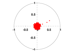
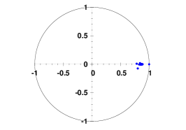
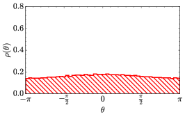
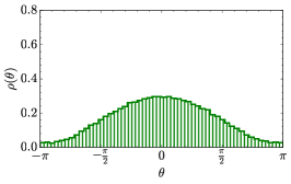
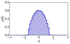
Figure 1: The Polyakov loop scatter plot (top) and its eigenvalue distribution (bottom) with $\hat{\mu}=2,N=32$ for temperatures $\hat{T}=0.8$ (red), $0.913$ (green) and $1.3$ (blue). The eigenvalue distribution for these temperatures corresponds to uniform, non-uniform, and gapped phases, respectively.

2 Phase Diagram

In Fig. 1(top), we show the Polyakov loop scatter plots for a fixed deformation mass $\mu=2.0$ for different temperatures. The corresponding eigenvalue distributions of the Polyakov loop are also shown in Fig. 1(bottom). For different values of the deformation parameter used, we calculated the transition point. In Fig. 2, we show the corresponding phase diagram.

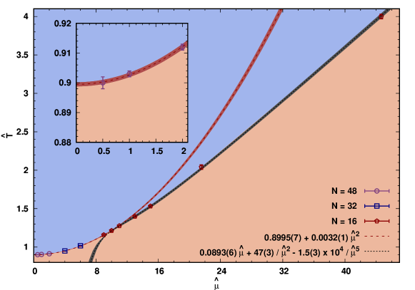
Figure 2: The $\hat{T}$ - $\hat{\mu}$ phase diagram of the bosonic BMN model from our $N_{\tau}=24$ results. The blue-shaded region in the diagram represents the deconfined phase, and the red-shaded region represents the confined phase.

This phase diagram smoothly interpolates between the limits of the bosonic BFSS model and the gauged Gaussian model with first order phase transition for all couplings, $g=\lambda/\mu^{3}$. The comprehensive analysis of this work can be found in Ref. [1]. The results for the critical temperature over extreme coupling regimes ($g=0$ and $g\rightarrow\infty$) match with previous studies [2, 3], and our analysis shows that these extreme regimes can be connected using a smooth function.

3 Future Directions

We plan to continue exploring the strong coupling regime ($g\rightarrow\infty$) with the larger values of $N$ to verify the results with other studies. We also plan to study the ungauged versions of the bosonic and the full BMN models.

4 Acknowledgments

We thank Raghav Jha for fruitful discussions and collaboration on this work. NSD thanks the Council of Scientific and Industrial Research (CSIR), Government of India, for the financial support through a research fellowship (Award No. 09/947(0119)/2019-EMR-I). The work of AS was partially supported by an INSPIRE Scholarship for Higher Education by the Department of Science and Technology, Government of India. AJ was supported in part by IISER Mohali and the University of the Witwatersrand. DS was supported by UK Research and Innovation Future Leader Fellowship MR/S015418/1 and STFC grant ST/T000988/1. Numerical calculations were carried out at the University of Liverpool and IISER Mohali.

References

- [1] Navdeep Singh Dhindsa et al. “Non-perturbative phase structure of the bosonic BMN matrix model” In JHEP 05, 2022, pp. 169 DOI: 10.1007/JHEP05(2022)169
- [2] Ofer Aharony et al. “The Hagedorn - deconfinement phase transition in weakly coupled large N gauge theories” In Adv. Theor. Math. Phys. 8, 2004, pp. 603–696 DOI: 10.4310/ATMP.2004.v8.n4.a1
- [3] Georg Bergner et al. “Confinement/deconfinement transition in the D0-brane matrix model – A signature of M-theory?” In JHEP 05, 2022, pp. 096 DOI: 10.1007/JHEP05(2022)096