Multiobjective Evolutionary Component Effect on Algorithm behavior

Abstract.

The performance of multiobjective evolutionary algorithms (MOEAs) varies across problems, making it hard to develop new algorithms or apply existing ones to new problems. To simplify the development and application of new multiobjective algorithms, there has been an increasing interest in their automatic design from their components. These automatically designed metaheuristics can outperform their human-developed counterparts. However, it is still unknown what are the most influential components that lead to performance improvements. This study specifies a new methodology to investigate the effects of the final configuration of an automatically designed algorithm. We apply this methodology to a tuned Multiobjective Evolutionary Algorithm based on Decomposition (MOEA/D) designed by the iterated racing (irace) configuration package on constrained problems of 3 groups: (1) analytical real-world problems, (2) analytical artificial problems and (3) simulated real-world. We then compare the impact of the algorithm components in terms of their Search Trajectory Networks (STNs), the diversity of the population, and the anytime hypervolume values. Looking at the objective space behavior, the MOEAs studied converged before half of the search to generally good HV values in the analytical artificial problems and the analytical real-world problems. For the simulated problems, the HV values are still improving at the end of the run. In terms of decision space behavior, we see a diverse set of the trajectories of the STNs in the analytical artificial problems. These trajectories are more similar and frequently reach optimal solutions in the other problems.

1. Introduction

Multiobjective Optimization Problems (MOPs) are problems with two or more conflicting objective functions that are optimized simultaneously. Several multiobjective evolutionary algorithms (MOEAs) have been proposed to solve MOPs (Deb et al., 2002; Beume et al., 2007; Zhang and Li, 2007), and for each of these algorithms several variants also have been designed, where some of the components of the algorithms are modified.

Recently, there has been an increasing interest in the automatic design of MOEAs (Radulescu et al., 2013a; Nebro et al., 2019; Bezerra et al., 2015b). In these approaches, a configurator recombines components of established MOEAs, creating more effective variants. However, the specific reasons for these improvements are still not clear. We argue that by understanding how specific components contribute to the performance of the variants, we can develop new and better components.

In this work, we investigate the question of how to measure the contribution of specific components in a MOEA. We focus this investigation on understanding the changes of anytime behavior effected on the algorithm by one or more components. We define anytime behavior as the grouping of the algorithm’s performance in terms of objective space convergence, and the choices made during the exploration of the decision space. We highlight that this definition focuses on the behavior of the algorithm when optimizing a problem, thus dissociating from landscape analysis, which focuses on the structure of the search space.

To analyze the contributions of specific components, we perform a case study on a variant of the MOEA/D algorithm (Zhang and Li, 2007) created by an algorithm configurator (irace). The MOEA/D is a popular and efficient algorithm for solving MOPs and can modify its search behavior on different MOPs.

To understand the contribution of each component, we perform modifications of the above automatically designed MOEA/D (auto-MOEA/D), by either removing a component, or replacing the component with the corresponding original in MOEA/D, as appropriate. For each modification, we investigate its performance on a set of problems to identify the contribution of the component. The methodology is an extension of our work introduced in (Lavinas et al., 2022c), with the inclusion of objective space behavior analysis in the form of anytime hypervolume analysis.

This investigation takes the form of a case study on six real-world analytical continuous benchmark problems, compiled together by Tanabe et. al (Tanabe and Ishibuchi, 2020) and two simulated continuous benchmark problems: (1) the problem of selecting landing sites for a lunar exploration robot (Nishiyama et al., 2015) and (2) the problem of optimization of car designs (Kohira et al., 2018). We conduct our analysis focusing on how these metaheuristics explore both the objective and decision space. Furthermore, we contrast the automatically designed MOEA (auto-MOEA/D) against each of the variants in terms of their Search Trajectory Networks (STNs) (Ochoa et al., 2021; Lavinas et al., 2022a); the diversity of their populations and the traditional performance metrics. Moreover, we compare the analytical and simulated problems in terms of the overall metrics of auto-MOEA/D. Finally, we analyze the similarities between the benchmark problems used for designing auto-MOEA/D and the real-world problems. To the best of our knowledge, this is the first component-wise analysis of MOEAs on the objective and decision space dynamics in real-world constrained MOPs. For reproducibility purposes, all the code and experimental scripts are available online at https://doi.org/10.5281/zenodo.8192256. In this paper, our contributions can be summarised as follows:

• We extend our previous study on behavior analysis to a more thorough investigation, by considering the differences in behavior in both the objective space and decision space during the search progress.

• We study the behavior of the components of MOEA/D in analytical and simulated real-world problems.

• We analyze the similarities between the benchmark problems used for designing auto-MOEA/D and the real-world problems.

The paper is organized as follows. Section 2 overviews previous work related to the automated design of algorithms and constrained problems. Section 3 introduces relevant concepts followed by Section 4 that explains the details of the methodology used in this work. The automatic design of the MOEA is shown in Section 5. Then, the comparison of the components set-up is presented in Section 6, and the analysis of the search behaviors dynamics of the different MOEA/D variants is shown in Section 7. Finally, Section 8 outlines our main findings, limitations and suggestions for future work.

2. Related Work

2.1. Analysis of Algorithm Behavior

Convergence analysis (Eiben and Schippers, 1998) is a way to describe algorithm behavior, by illustrating the trade-off between exploration and exploitation in evolutionary algorithms. However, the information of whether a population has converged or not does not inform the location of this convergence, hence it does not allow the user to know whether the convergence is premature or not. In this way, understanding the behavior of search and optimization algorithms remains a challenge.

Another way to understand the behavior of an algorithm, especially in the case of multiobjective optimization, is to visualize and contrast the Pareto front achieved by the algorithm (Fonseca and Fleming, 1996a, b; Kerschke and Grimme, 2017; Schäpermeier et al., 2020; Liefooghe et al., 2018; Fieldsend and Alyahya, 2019). However, in general this approach focuses on detecting increments in performance, and limits to observing changes in the objective space dynamics. We argue that analysing the decision space might expand our understanding of the behavior of the multiobjective optimisation solvers.

Finally, another way to understand algorithm behavior is through Search Trajectory Networks (STNs) (Ochoa et al., 2020, 2021), which illustrate as a graph how the algorithm explores the decision space. Recently, STNs were generalized to multiobjective algorithms (Lavinas et al., 2022a), and we use these MOP-STN models as one of the tools to discriminate behavior changes in MOEA components.

2.2. Automatic Design of Evolutionary Algorithms

Most approaches to the automatic design of evolutionary algorithms focus on creating templates that can instantiate many algorithms and their parameter settings for performance improvements. For example, there have been studies to automatically design NSGA-II (Nebro et al., 2019) and MOEA/D (Bezerra et al., 2015b) on commonly used benchmark sets. Moreover, two seminal examples are the works of Bezerra et al. (Bezerra et al., 2016, 2020a), which proposed a component-wise MOEA template that instantiates multiple existing frameworks for continuous and combinatorial optimisation MOPs. Their research efforts mainly focus on exploiting the automatic configuration to increase the performance of multiobjective algorithms in benchmark problems without constraints.

We also highlight the work of Radulescu et al. (Radulescu et al., 2013a), which focuses on improving the performance of multiobjective metaheuristics. These works are insightful approaches; however, they concentrate on finding well-performing configurations of multiobjective algorithms. On the other hand, there are few studies in the context of the automatic design of algorithms that focus on the effect of the different components on the performance of the algorithm.

2.3. Behavior Analysis in the Continuous Multiobjective Domain

There are few works in the continuous multiobjective domain related to behavior analysis. Some of the few examples with works on the relations between behavior and population size (Joshi and Deshpande, 2014) and between behavior and solution quality and time (Radulescu et al., 2013b). In contrast more works studied the behavior of multiobjective algorithms in the combinatorial domain. Two of these works focus on understanding selection and population size effects on the algorithms’ ability in terms of dominance status, membership to the Pareto optimal set, recentness of discovery, and how their numbers change generation by generation (Hifi et al., 2021; Aguirre et al., 2014). Another work explores how the relationships of already known and controllable structures, such as modality and ruggedness to understand the working principles, behavior, and the performance of MOEAs (Aguirre and Tanaka, 2007). Finally, few studies have considered the contribution of individual components to MOEAs performance (Bezerra et al., 2016). Furthermore, in most cases, performance is evaluated in unconstrained problems or problems where constraints are simple to address (Tanabe and Ishibuchi, 2020; Bezerra et al., 2020b; Vaz et al., 2021). These constraints invalidate some solutions, which makes finding a set of feasible solutions a challenging task.

3. Preliminaries

MOEA/D (Zhang and Li, 2007) is a popular and efficient algorithm for finding good sets of trade-off solutions for MOPs. The key idea of MOEA/D is to create a linear decomposition of the MOP into a set of single-objective subproblems. Decomposing the MOP in various single-objective subproblems makes the algorithm very flexible for dealing with constraints because adding a penalty value is straightforward: MOEA/D adds a penalty value related to the amount of violation of the constraint for each of the subproblems. Given the nature of the single-objective subproblems, MOEA/D can easily use multiple constraint handling techniques (CHTs).

Algorithm 1 MOEA/D outline

1:Initialize population and decomposition vectors.

2:while Computational budget is not meet do

3:     Define Neighbourhood relations.

4:     If partial update is used, select subset of solutions to update.

5:     Else, all solutions are updated.

6:     Generate candidates from the updated solutions and their neighbors.

7:     Evaluate the candidates on their respective subproblems.

8:     Update the population using the candidates.

9:     Save non-dominated solutions in UEA.

10:     if restart criteria is met, regenerate the population.

11:end while

The MOEA/D template we propose for instantiating and designing variants of this metaheuristic is shown in Algorithm 1. We use the generational version of MOEA/D incremented with the Unbounded External Archive (UEA). The UEA is used to keep all nondominated solutions found by a multiobjective optimizer during the search process. Solutions in the archive are only used as the output of the algorithm and are stored in a way that they do not affect the search run (Bezerra et al., 2019; Tanabe et al., 2017).

3.1. Automatic Design Configurator

For automated design, we use Iterated Racing (irace) (López-Ibáñez et al., 2016). The goal of using irace is to be able to tune the set of components of an algorithm over a set of optimization problems to find a configuration that performs well on average in all problems. After fine-tuning the MOEA/D with irace, we conduct an ablation analysis (Fawcett and Hoos, 2016; López-Ibáñez et al., 2016) to help us understand the choice of components values and whether each of these choices effectively improves the MOEA/D performance. This analysis investigates the differences between configurations. We conduct an ablation analysis between a target configuration selected  and the best configuration found by irace.

3.2. Search Trajectory Networks (STNs) for MOPs

We use Search Trajectory Networks as a tool for visualization following the method described in (Lavinas et al., 2022a, c). In an STN model, each solution in the decision space is mapped to a location. Similar solutions are generally mapped to the same location, as the locations represent a partition of the decision space. The network models are extracted from data obtained during several runs of the studied algorithm(s). A network model requires defining its nodes and edges. In an STN model, nodes are the locations in the search trajectories visited by a given algorithm, and edges connects two consecutive locations in the trajectory. A strength of network models is that they can be visualized. When decorating the networks for visualization, it is possible to highlight attributes of the nodes and edges that are relevant to the search process. In these visualizations, the size of nodes and the width of edges are proportional to how many times the algorithms visited them during the aggregation of runs used to extract the model. Visualizations use force-directed graph layout algorithms as implemented in R package igraph (Csardi and Nepusz, 2006).

The key idea of this method is that we keep track of a small number of decomposition vectors, match a representative solution to a vector, and then merge the vector trajectories of each vector into a single multiobjective STN. The merged STN model merges the $n$ STNs of each decomposition vector and is obtained by the graph union of the $n$ individual graphs. The merged graph contains the nodes and edges present in at least one of the vectors graphs. Attributes are kept for the nodes and edges, indicating whether they were visited by both algorithms (shared) or by one of them only. Finally, we have the merged STN models, where different MOEAs are combined into one single merged STN model. The merged STNs allow us to directly visually compare how distinct variants explore the decision space (Lavinas et al., 2022c). In the merged models, there is the notion of shared nodes, which are nodes visited by more than one algorithm and are indicated in grey colour in the network visualization.

3.3. Network and Performance Metrics

We use the following STN metrics to assess the global structure of the trajectories and bring insight into the behavior of the MOEAs modelled. These metrics are (1) the number of unique nodes, (2) the number of unique edges and (3) the number of shared nodes between vectors and (4) the number of solutions in the Pareto front.

For reference, we use the following criteria to compare the results of the different strategies, based on the metric analysis done in the work of (Lavinas et al., 2022c): final approximation hypervolume (HV), the volume of the n-dimensional polygon formed by reference points and solutions. It is worth noting that additional network and MOP metrics could also be considered. These metrics are summarised in Table 1. We also use the population variance metric.

Table 1. Description of decision space metrics

Metric	Description
Nodes	Total number of nodes, which corresponds to the number of unique locations visited.
Edges	Total number of edges, the number of unique search transitions.
Variance	Dispersion of the population in the decision space.
#PF	Number of solutions in the theoretical Pareto front or in the best approximation to the Pareto front.

4. behavior Analysis Methodology

Here we define a methodology to measure the differences in decision and objective space dynamics of variants of an algorithm that alter a single component from the base algorithm. Our reason for using such methodology is to identify the most influential components of an algorithm and how they affect the search space dynamics in different problems. Thus, we can identify better the influence of the considered component, even if such method explores a reduced part of the possible algorithm versions.

First, we use irace to automatically design a tailor-suited MOEA (auto-MOEA) that performs well in a set of problems. Secondly, we modify auto-MOEA to create many variants and each one of these variants have only one component that differs from auto-MOEA. These variants are obtained by: (1) removing a component if possible; (2) otherwise, replacing this component with the corresponding one from the original MOEA. Thus, we have the multiple MOEAs: the auto-MOEA plus one variant for each component. The idea here is to be able to capture the effects of each one of the components individually. This step to create variants is done manually, based on the users expertise about the components.

Then, we collect log data of the executions of all variants and the base algorithm during their run in the problems of interest. This log data contains the parameters of the non-dominated solutions of each generation as well as their objective space values and the solution’s feasibility . This data is processed following the approach described in Subsection 3.2 for analysing how the components affect the decision space exploration of such MOEA. To measure the different behaviors, we use metrics and visuals from the Search Trajectory Networks (STNs) (Ochoa et al., 2021; Lavinas et al., 2022a) combined with a population diversity metric.

We also use the log data to calculate the anytime HV performance of the algorithm over the evaluations and the number of solutions in the Pareto front. To verify the impact of the variant, we calculate the difference value of the metrics of each variant to the auto-MOEA.

5. Designing auto-MOEA/D

We analyse the components of a MOEA/D instance that was automatically designed. This design process was done in a component-wise framework, similar to the protocols used by Bezerra et al. (Bezerra et al., 2016) and Campelo et al.  (Campelo et al., 2020). We extend the MOEADr package (Campelo and Aranha, 2018) to introduce options for population restart and the most representative Resource Allocation (RA) method, called the partial update of the population  (Lavinas et al., 2020, 2022b).

5.1. Variable Components Search Space

The configuration space used in our experiments contains the algorithm components and numerical parameters of the MOEA/D framework. These are shown in Table 2. Special attention is required with the variation operators: Differential Evolution (DE) mutation and polynomial mutation. They are always performed sequentially, first DE and then the polynomial mutation. Thus, the order of the stack of operators is kept fixed, but the parameter values are variable. Similar attention should be given to the restart strategy, where only the choice of using this strategy is explored.

Table 2. Components search space.

Component	Domain
Decomposition vector generator	Uniform or Sobol(Zapotecas-Martínez et al., 2015)
Population size	100 or 500
Aggregation function	Weighted Tchebychef or
	Adjusted weighted Tchebychef
Update strategy	Best, $nr=[1,20]$
	Restricted, $Tr=[4,20]$
Neighbourhood function	$T=[10,100]$
	$Delta=[0.1,1]$
DE mutation	$F=[0.1,1]$
Polynomial mutation	$\eta_{m}=[1,100]$
	$prob=[0,1]$
RA (Partial update strategy)	True $n={0.10,0.15,0.20,0.25}$
	False, not used
Restart strategy	True, every $20000$ evaluations
	False, not used

We choose to fix some MOEA/D components to reduce the search space for the irace configurator. The fixed components are the computational budget, the objective scaling and the constraint handling technique (CHT). These fixed components are always present in every configuration of the MOEA/D that irace generates: (1) the number of functions evaluations is set to $100000$ in order to grasp all possible behaviors of the automatically designed algorithm during the run; (2) all objectives were linearly scaled at every iteration to the interval $\left[0,1\right]$; (3) we use the Dynamic CHT (Joines and Houck, 1994), which starts with a small penalty value, increases it across the iterations to focus on the diversity of feasible solutions, and then later focus on the convergence of those solutions. It is defined by $f^{agg}_{penalty}(x)=f^{agg}+(C*t)^{\alpha}*v(x)$, where $C=5$ and $\alpha=2$ are constants we defined based on the following works (Joines and Houck, 1994; Vaz et al., 2021), $t$ is the generation number and $v$ is the total violation of a solution.

5.2. Configurator Setup

We use the irace configurator (López-Ibáñez et al., 2016) to automatically assemble and design a MOEA/D configuration based on the components available in the MOEADr package extended with the options for population handling mentioned above. We run irace with its default settings, except for the number of elite configurations tested, which we increase from 1 to 7, following Campelo et al. work (Campelo et al., 2020). We run irace with a budget of $15000$ runs.

5.3. Benchmark Problems for Configuration

We use the DASCMOP benchmark set (Fan et al., 2020) to design the auto-MOEA/D. This set has nine constrained test functions: DASCMOP1-6, each with eleven constraints, and DASCMOP7-9, each with seven constraints. The constraints can be modified to consider three types of difficulties: type-I considers diversity-hardness, type-II considers feasibility-hardness and type-III considers convergence-hardness. More information about the problems and these difficulty triplets can be found in (Fan et al., 2020). We use the implementation of the test problems available from the Pymoo python package (Blank and Deb, 2020). To have a more balancing training function set, we change the hardest constraints difficulty triplet, numbered 16, from our previous work (Lavinas et al., 2022c), to a set of triplets ranging from low to high difficulty and numbered 4, 8, 12 and 16.

5.4. Benchmark Problems for Behavioral Analysis

The real-world analytical multiobjective optimization problems used were selected from the new test suite introduced by Tanabe et. al (Tanabe and Ishibuchi, 2020): (1) bar truss design (CRE21), the objectives are to minimize the structural weight and displacement resulting from the joint; (2) design of welded beams (CRE22), the objectives are to minimize the cost and the final deflection of the welded beams; (3) disc brake design (CRE23), the objectives are to minimize brake mass and decrease downtime; (4) side impact design of the car (CRE31), the objectives are to minimize the average weight of the car, the average speed of the column V responsible for supporting the impact load and the force experienced by a passenger; (5) conceptual submarine project (CRE32), the objectives are to minimize the cost of transportation, the weight of the light vessel and the annual cargo transport capacity; (6) water resource planning (CRE51), the objectives are to minimize the cost of the drainage network, the cost of installing the storage center, the cost of installing the treatment center, the expected cost of flood damage and the expected economic loss due to the flood.

The real-world simulated MOPs used are the two recently proposed problems by the Japanese evolutionary computing society: (1) Mazda benchmark problem (MAZDA): this is a discrete optimizing problem to design MAZDA cars, where the objectives are to maximize the number of parts common to three different cars and minimize the total weight of the car (Kohira et al., 2018); (2) lunar landing site selection (MOON): the goal is to select landing sites coordinates (x,y) for a lunar exploration robot to land with the objectives of minimizing the number of continuous shaded days, minimizing the inverse of the total communication time , and minimizing the tilt angle (Nishiyama et al., 2015).

5.5. Evaluation Metrics for the Automatic Design

Analysing MOP solvers considering only their final approximation provides limited information related to these algorithms’ performance since any MOP solver should return a suitable set of solutions at any time during the search (Zilberstein, 1996; Radulescu et al., 2013b; Dubois-Lacoste et al., 2015; Tanabe et al., 2017). Here, we analyse the anytime performance effects in terms of hypervolume (HV) values to investigate the impact of different configurations of MOEA/D on their Unbounded External Archive. We run auto-MOEA/D 10 times on each of the problems.

We use the following method to compare the results of the different strategies: we calculate the accumulative HV over the search progress to quantify the HV anytime performance. At every $1000$ evaluations, we calculate the HV of the solutions in the UEA at that iteration, using the reference point as: 11, over the number of objectives; following the work of Bezerra et al. (Bezerra et al., 2016). Then, we sum all values to have an approximated evaluation of the anytime HV curve.

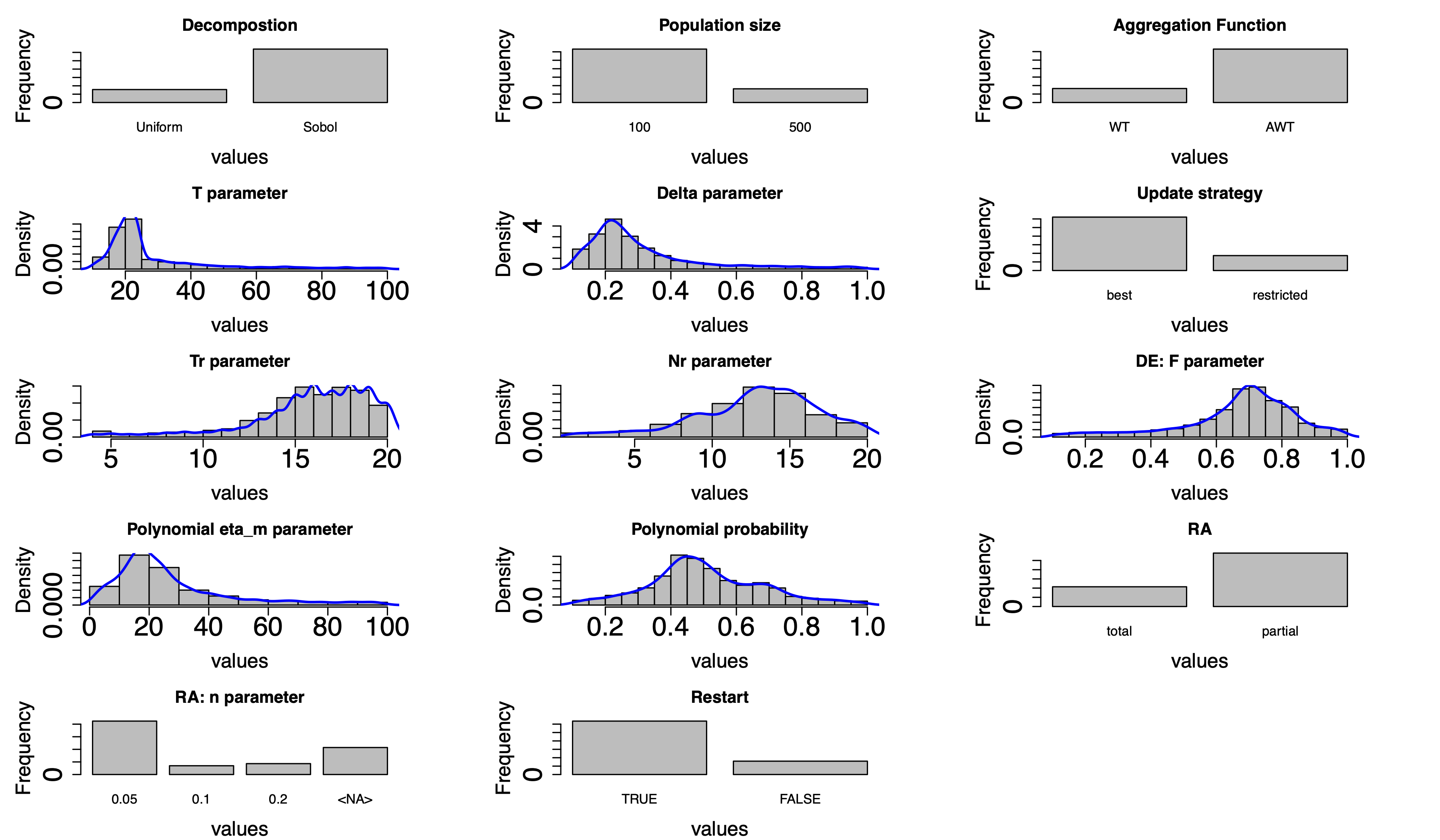
Figure 1. irace output with the frequency of the different choices of components and parameters.

Figure 1 shows the frequency of the different choices of components and parameters after the tuning and ablation design is performed. As in (López-Ibáñez et al., 2016), the ablation analysis is done to better use the available computational resources, focusing on better-performing configurations found by an automatic configuration method, and proceeds by changing one parameter at a time, focusing more on well-performing configuration, instead of more common useful configurations.

There is a consensus over the components and parameters studied here. This suggests that irace is confident that the choice of components used in the auto-MOEA/D design has at least an adequate overall performance in the problems used during the configuration process.

5.6. Performance of auto-MOEA/D

Here, we briefly describe the performance of auto-MOEA/D in terms of HV  and variance of the final population, and the STNs metrics: number of nodes, edges and shared nodes. For the calculation of HV, the objective function was scaled to the (0, 1) interval, with the reference point of $1.1$, repeated over the number of objectives. Thus, the maximum HV is $1.21$ for MOPs with two objectives or $1.331$ for MOPs with three objectives after scaling the values. Instead of showing the achieved HV value of the auto-MOEA/D, we calculate how close the performance of this algorithm is to the maximum possible HV value (max(HV)). Values close to 0 indicate no HV performance  while values close to 1 indicate high performance.

Table 3. hypervolume ratio (HV)/max(HV), HV Standard Deviation, Standard Deviation, Nodes, Edges, population variance, and the number of solutions in the theoretical Pareto front ($\#PF$) of the auto-MOEA/D for the DASCMOP problems.

	auto-MOEA/D
MOP	HV/max(HV)	SD	Nodes	Edges	Variance	$\#PF$
DASCMOP1	0.931	0.002	4268	4812	0.514	212
DASCMOP2	0.964	0.002	4821	5480	0.45	279
DASCMOP3	0.962	0.007	7175	8595	0.494	44
DASCMOP4	0	0	2316	2890	4.812	0
DASCMOP5	0.095	0.362	2352	2998	5.089	0
DASCMOP6	0	0	2313	2901	5.022	0
DASCMOP7	0.035	0	2388	3139	5.035	0
DASCMOP8	0	0	2465	3235	4.372	0
DASCMOP9	0.849	0.397	15756	19233	0.437	10
MOON	0.392	0.452	1375	3012	0.007	2
MAZDA	0.016	0.026	5443	5531	5.366	0
CRE21	0.989	0.011	4774	6370	0.1	0
CRE22	0.995	0.001	2047	2192	0.119	12
CRE23	0.608	0.003	7774	10369	0.335	1
CRE31	0.567	0.002	5259	5497	0.72	2
CRE32	0.756	0.011	14976	17743	0.331	0

The different metric values for the auto-MOEA/D are shown in Table 3. We can see that higher HV values correspond to a high number of nodes and edges and lower final populational variance values for the DASCMOP1, DASCMOP2, DASCMOP3 and DASCMOP9 problems. In contrast, the opposite happens for the other DASCMOP problems. Given the low HV performance, we speculate that auto-MOEA/D has a premature convergence probably to local optima areas of the decision space.

The HV performance of auto-MOEA/D deteriorates for the simulated MOON and MAZDA problems. There is no agreement in values of the number of nodes, edges and variance found for auto-MOEA/D in this set of problems, suggesting that each problem has different features in relation to the other. Interestingly, the number of nodes and variance metrics are the lowest in the MOON problem which might suggest that the population gets trapped in local optima during the run. This could also explain partially why the HV performance is low. For the MAZDA problem auto-MOEA/D also has a poor HV performance, but a higher number of nodes, edges and variance in comparison to the MOON problem.

For the CRE problems, we see that the HV performance is close to the DASCMOP1, DASCMOP2, DASCMOP3 and DASCMOP9 problems. In general, the other metrics follow a similar comparison trend between CRE problems and DASCMOP. Thus, we understand that there are similarities among the artificial DASCMOP problems and the CRE problems and limited similarities with the more challenging simulated MOON and MAZDA problems.

Finally, we comment about the results on constraint difficulty change between our previous work and this current study. On contrary to our expectations, having different constraints difficulty levels lead to improvements the HV performance of auto-MOEA/D in the easy problems (DASCMOP1-3 and 9), but no clear increments in performance for the hard set of problems (DASCMOP4-8).

6. Comparison of the Components

Here we use our methodology to investigate the effects of the final configuration of a machine-designed multiobjective algorithm. This analysis aims to measure the differences in the decision and objective space dynamics among several variants from the MOEA and, through these measures, identify the most influential components of the automatically designed algorithm.

Table 4. Auto-MOEA/D setup and the variants under analysis. For each variant, only one component is changed, while the other components are the same as auto-MOEA/D.

Auto-MOEA/D setup, and its Variants
auto-MOEA/D	Component variant
Decomposition + pop. size	Decomposition + pop. size
$Sobol,100$	$SLD,300$
Aggregation function	Aggregation function
$AWT$	$WT$
Update	Update
$Best$	$Restricted$
$nr=9$	$nr=2$
Neighbourhood pars.	Neighbourhood pars.
$T=22$	$T=20$
$Delta=0.9822$	$Delta=0.9$
Operators pars.	Operators pars.
$DE:F=0.4908$	$DE:F=0.5$
Polynomial: $\eta_{m}=80.9844$	Polynomial: $\eta_{m}=20$
Polynomial: $prob=0.4556$	Polynomial: $prob=0.3$
Restart	Restart
$True$	$False$
RA	RA
$Partial,5\%$	$False$

To analyse these behavioral effects of the different variants, we compare the auto-MOEA/D described in Section 5 against variants with at most one single component altered. We obtain these variants by changing or removing a single component of the auto-MOEA/D at a time. This is done by either (1) removing the component from the algorithm when possible or (2) changing its parameters to its counterpart in the traditional MOEA/D.

Table 4 lists the auto-MOEA/D on the left side, which is generated by the algorithm in section 4, and the variants on the right side. These variants are not necessarily components generated by auto-MOEA/D. When total removal of the component is not possible, we use the standard version of these components introduced by Hui Li and Qingfu Zhang in MOEA/D-DE (Li and Zhang, 2009), and commonly found in the literature. Thus; there are seven variants to analyse, which added to auto-MOEA/D itself least to a total of eight algorithmic variations of the MOEA/D framework. These variations are compared quantitatively and visually in terms of their STN models to detect which components procude the most extensive changes.

7. behavioral dynamics

To quantitatively analyse the dynamics of the search progress of the different variants of MOEA/D, we model the search dynamics using STNs for each pair of auto-MOEA/D and an auto-MOEA/D variant, leading to seven different pairs. We highlight that given the lower impact on performance of the decomposition and population size observed on the original paper (pre-extension, see (Lavinas et al., 2022c)) and since that most works on the literature focus on population size and decomposition methods(to name only a few (Joshi and Deshpande, 2014; Lavinas et al., 2022b; Aguirre et al., 2014; Hifi et al., 2021; Bezerra et al., 2015a)), we combine these components into one, and direct our studies towards the other components.

We base our quantitative analysis on the traditional multiobjective metrics hypervolume (HV); the number of: nodes, edges and shared nodes of the STN models; and the populational variance. For the HV, we use the reference point of 1.1, repeated over the number of objectives. We linearly scaled all objectives to the interval $[0,1]$, for a more straightforward comparison among the algorithms. We run each variant 10 times on each of the problems.

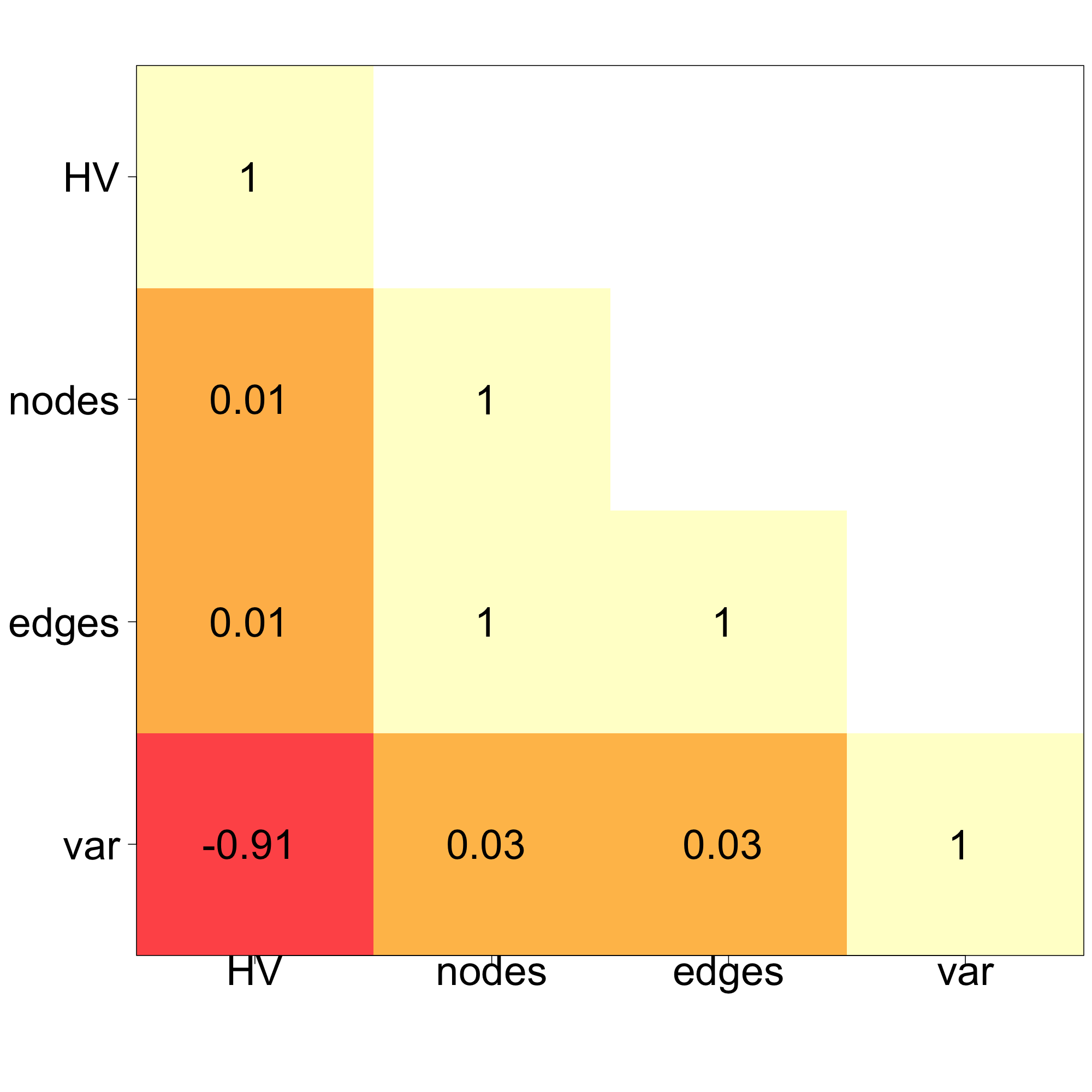
((a)) DASCMOP problems.

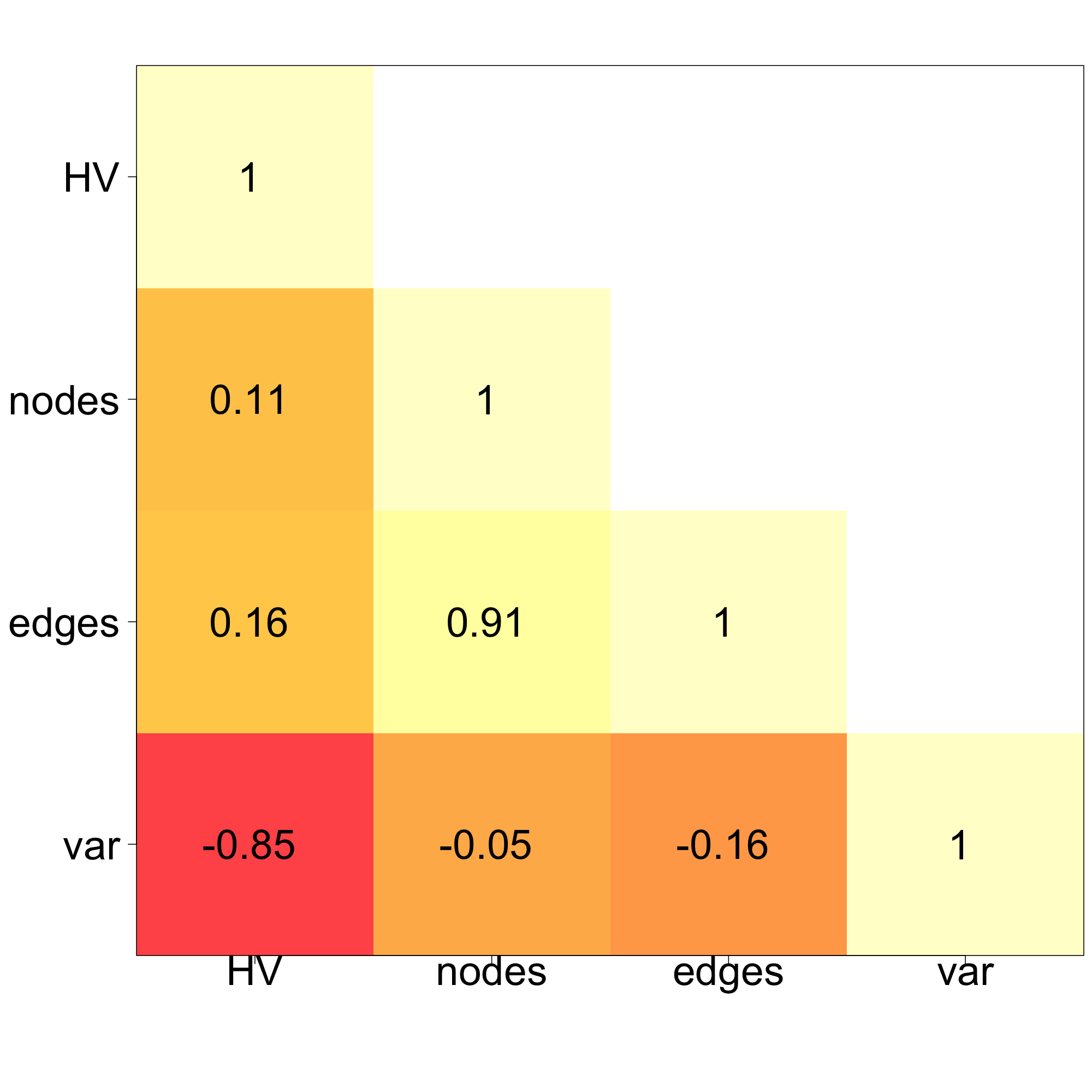
((b)) Simulated problems.

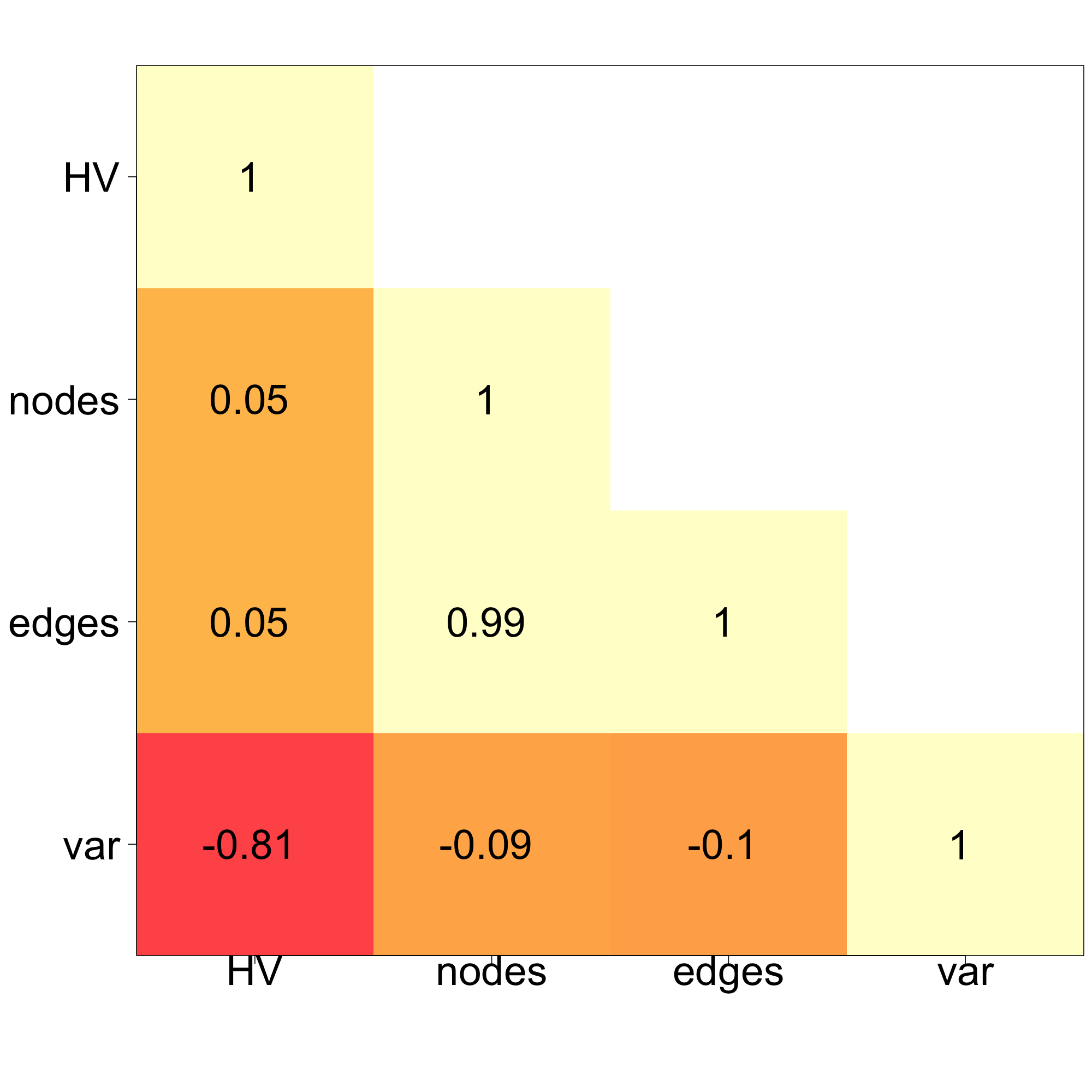
((c)) Analytical problems.

Figure 2. Correlation matrix among the different metrics. We find some correlation among HV and variance of the final population; and correlation between the number of nodes and edges.

7.1. Metrics Analysis

Figure 2 shows the correlation matrix among the different metrics studied, considering the results of the MOEA/D variants for the DASCMOP, simulated  and analytical  problems. Since the number of nodes and edges have a high correlation, we remove the number of edges metric from our analysis. The other STN metrics, together with the final population variance are on the decision space analysis; thus, we use them in our following analysis to strengthen the study. Furthermore, we see a correlation between the HV metric and the population variance. This correlation suggests a link between this decision space metrics and HV increments of performance. Moreover, we understand that there might exist a connection between solution diversity, represented by the variance, and overall performance and that this connection is problem-independent.

7.2. Objective Space Behavior

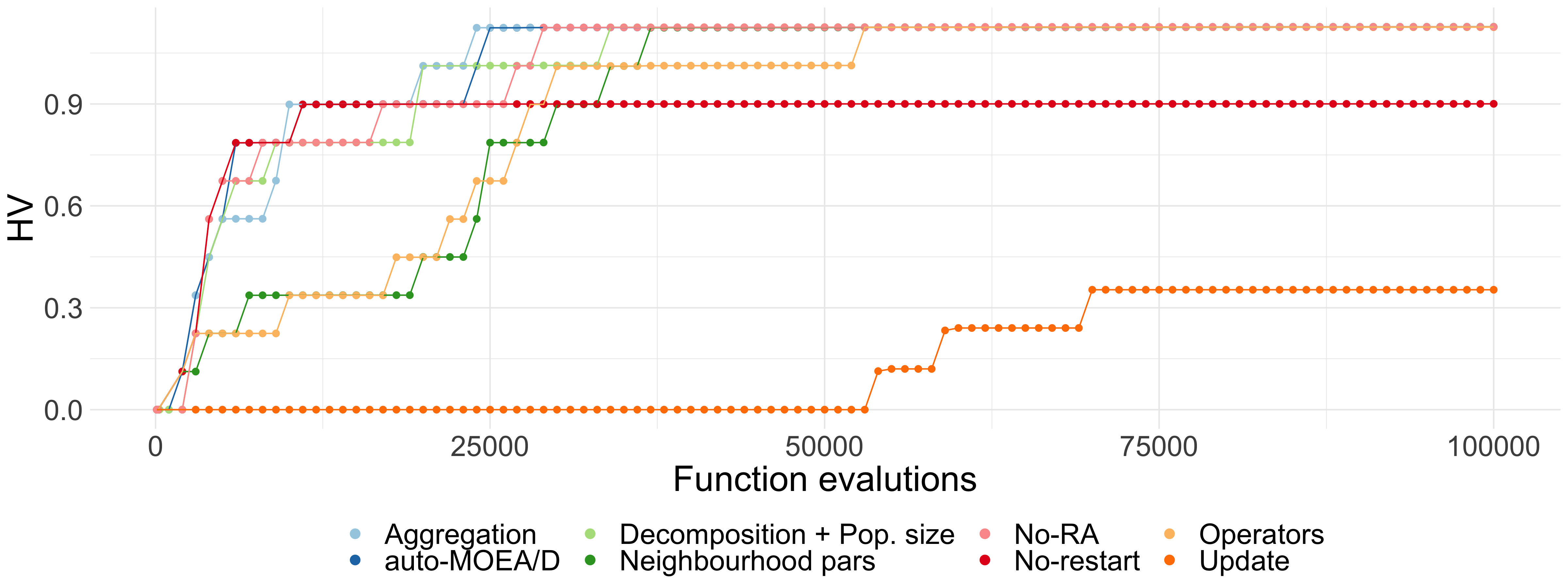
Figure 3. DASCMOP1 - HV anytime performance of auto-MOEA/D and its variants. The update strategy and not using restart lead to worse performance.

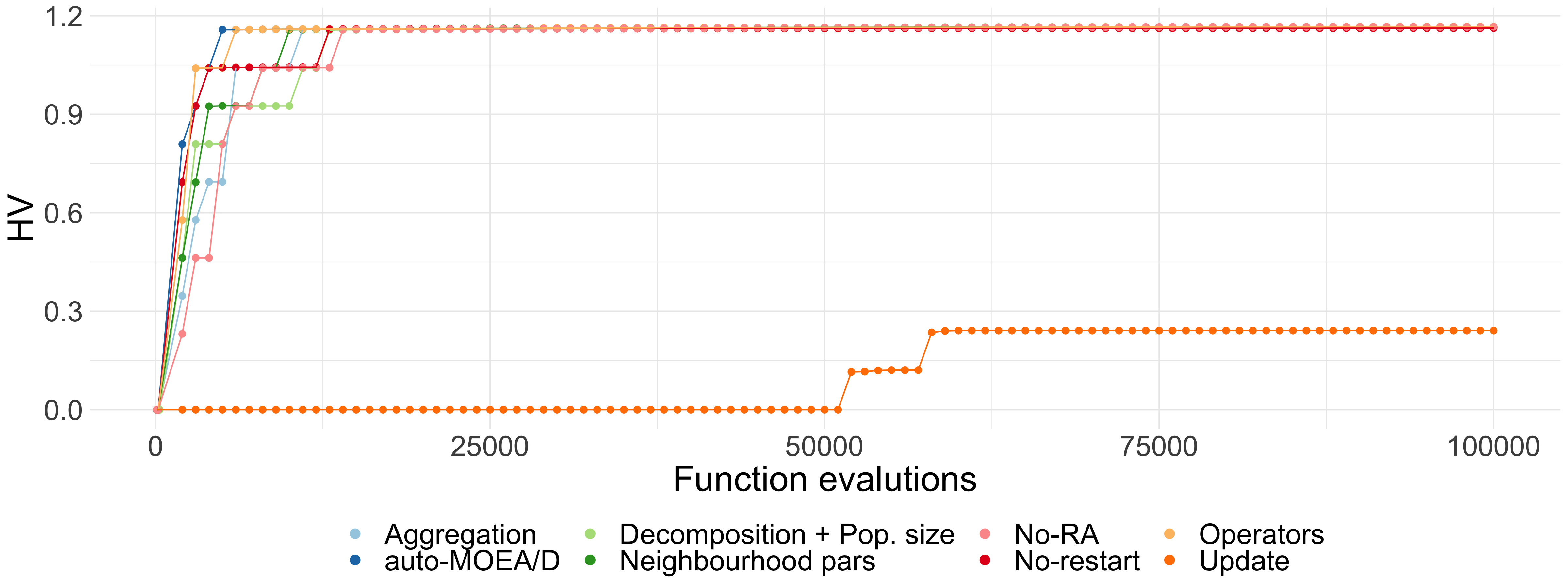
Figure 4. DASCMOP2 - all variants converge to the maximum HV, with the exception of the update strategy.

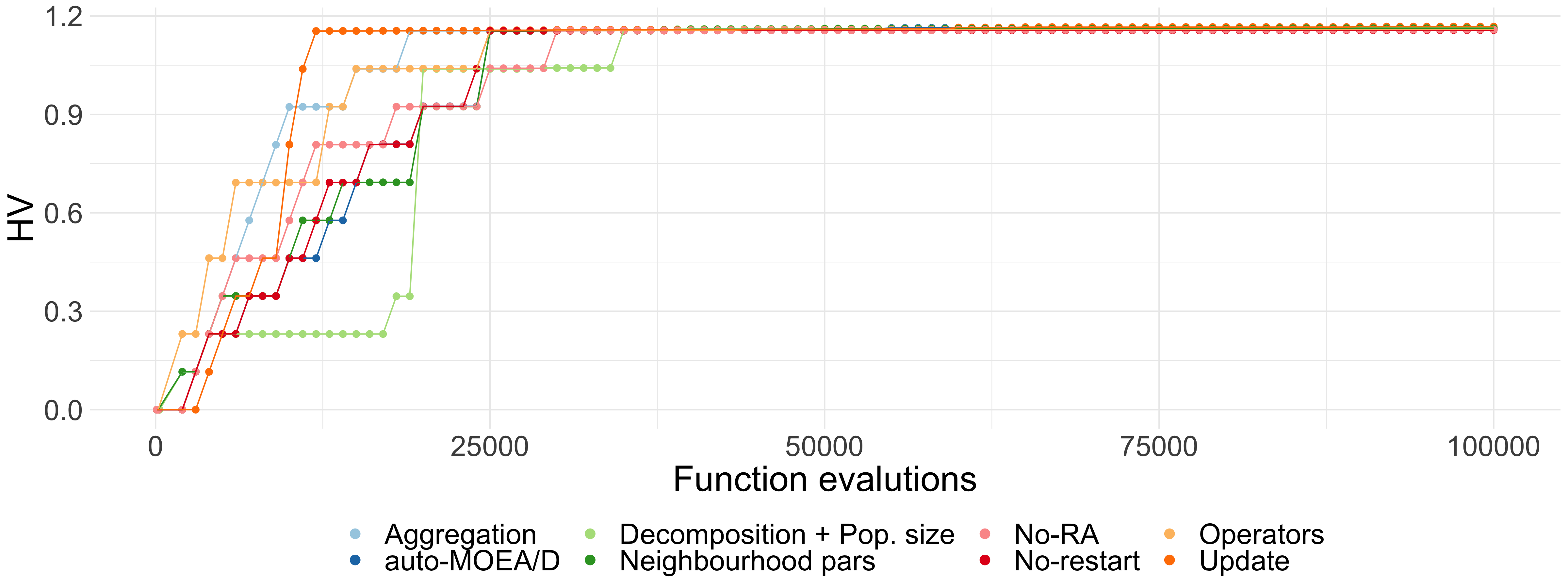
Figure 5. DASCMOP3 - all variants converge to the maximum HV before half of the search.

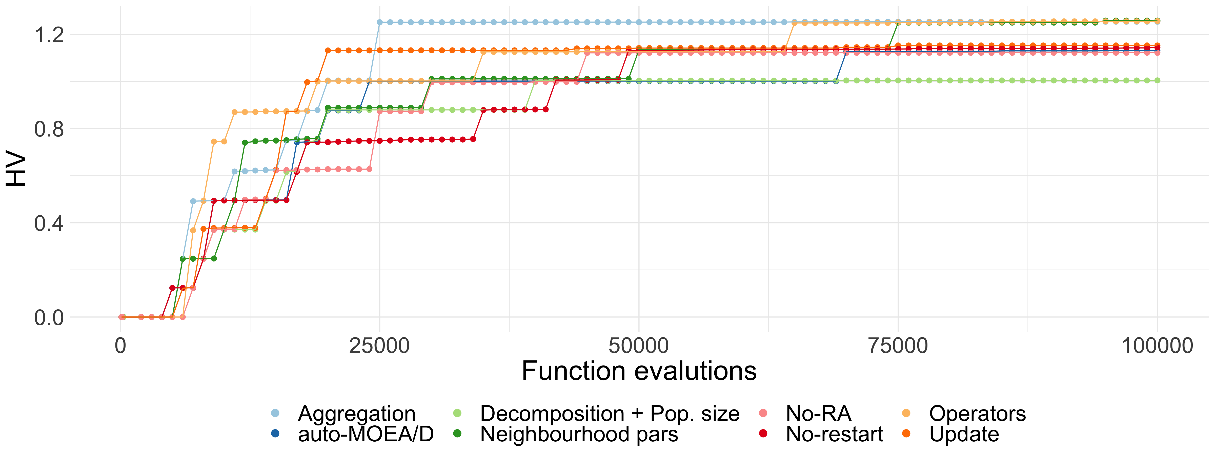
Figure 6. DASCMOP9 - the aggregation variant converges to high HV values faster than the other variants.

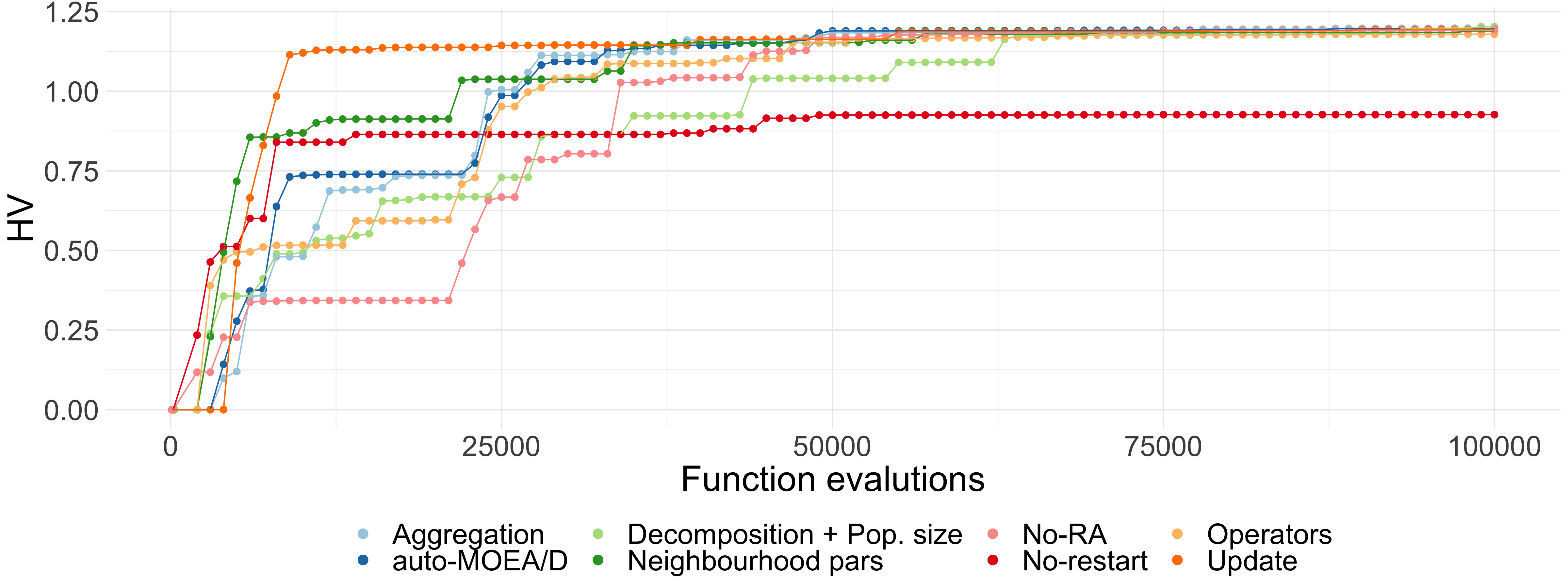
Figure 7. CRE21 - the variants converge to about the same HV value, with the exception of the no-restart.

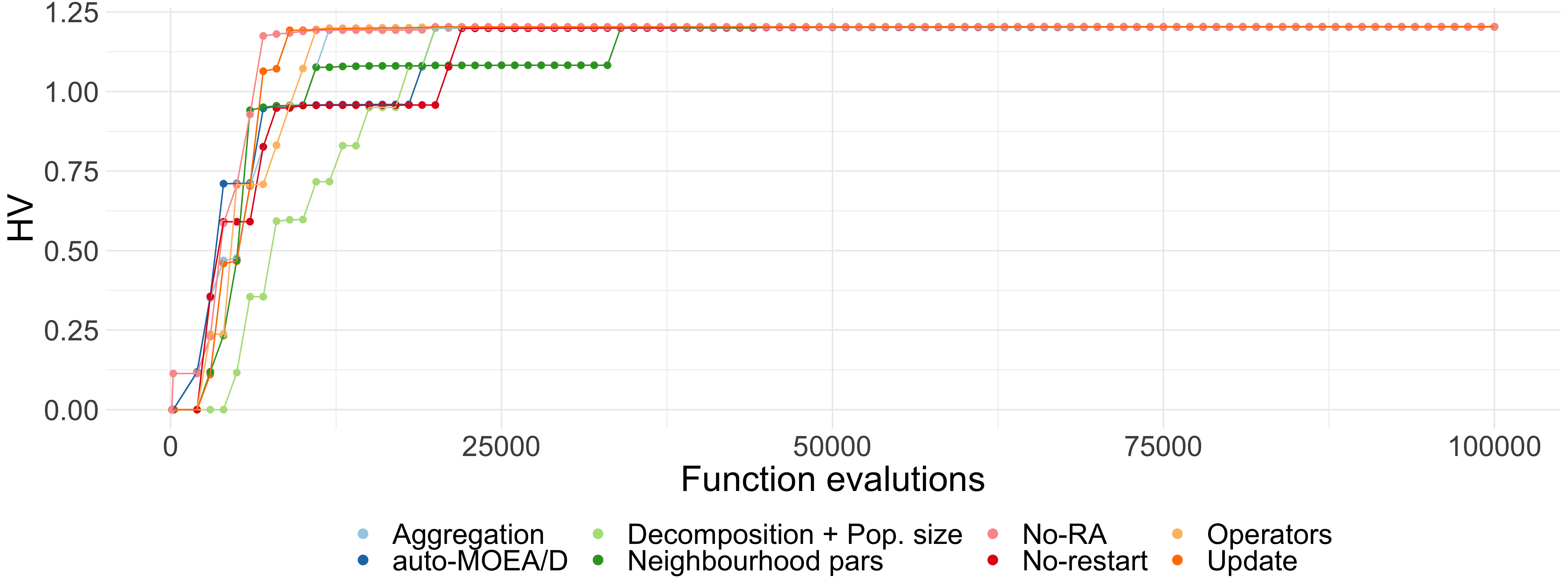
Figure 8. CRE22 - all variants converge to maximum HV at about one third of the search.

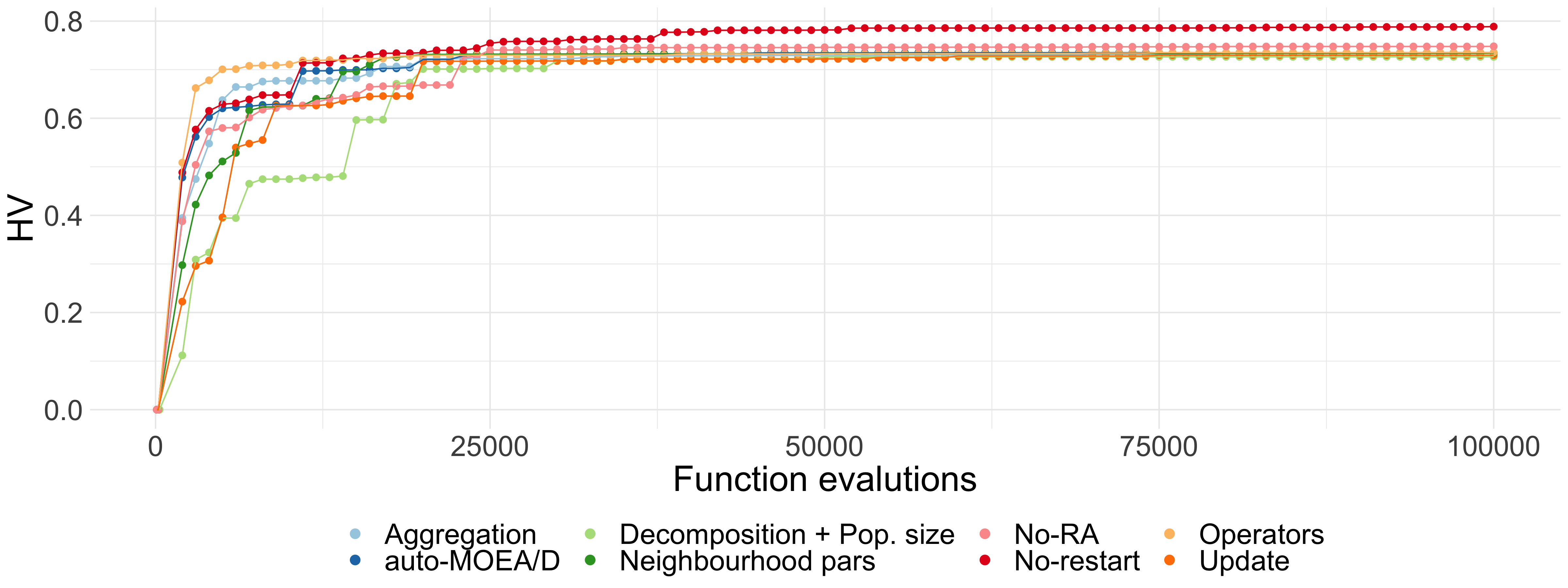
Figure 9. CRE23 - the variants converge to sub-optimal HV values at about one third of the search.

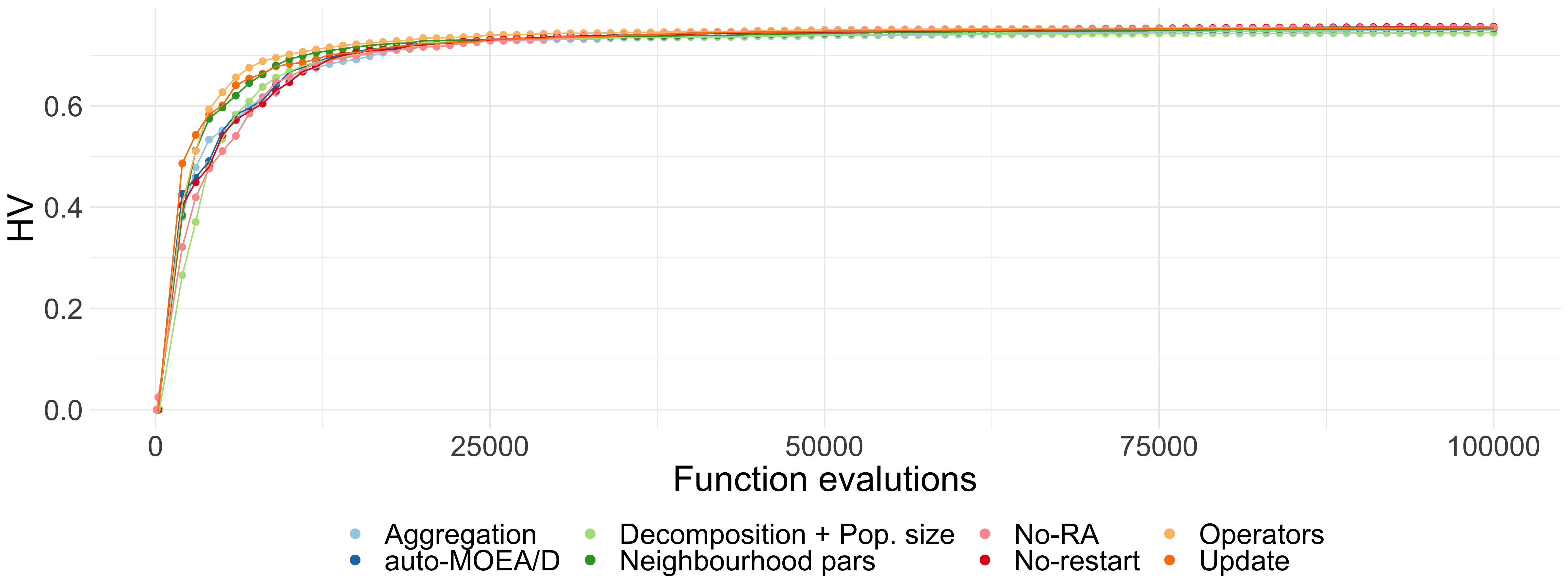
Figure 10. CRE31 - similarly for CRE23, the variants converge to sub-optimal HV values at about one third of the search.

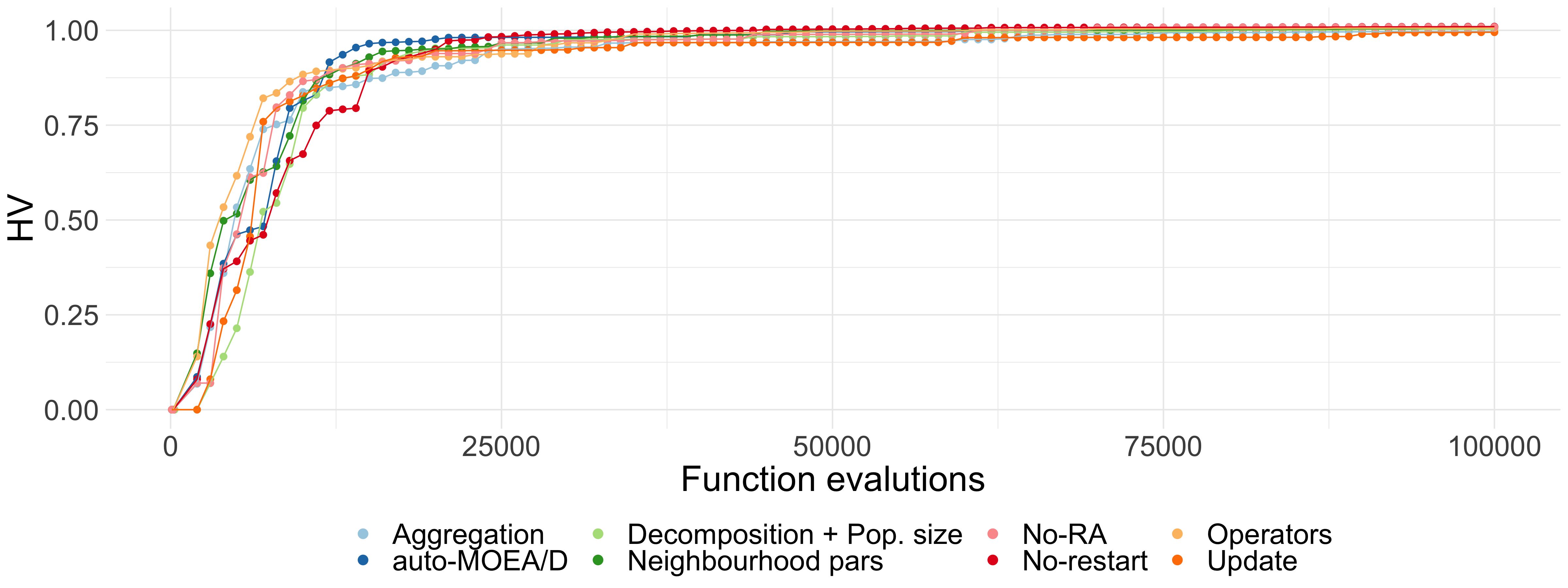
Figure 11. CRE32 - Better performance than CRE31, but the variants again converge early to sub-optimal values.

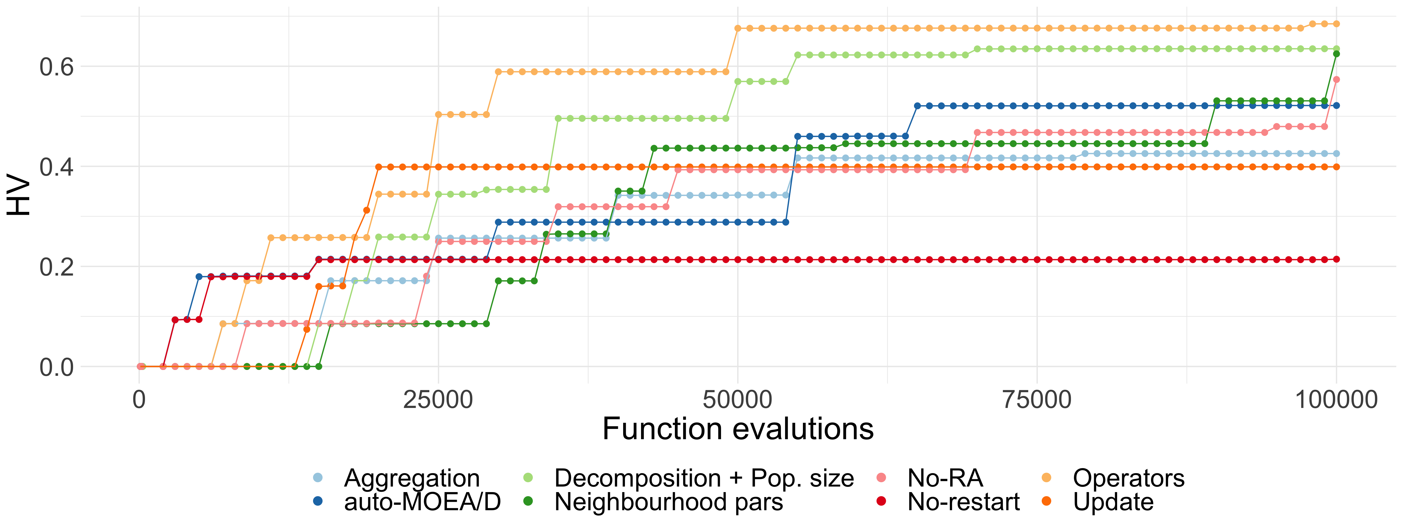
Figure 12. MOON - the HV values are much different among the variants, with the operators variant achieving the best results and not-restarting has a big negative impact.

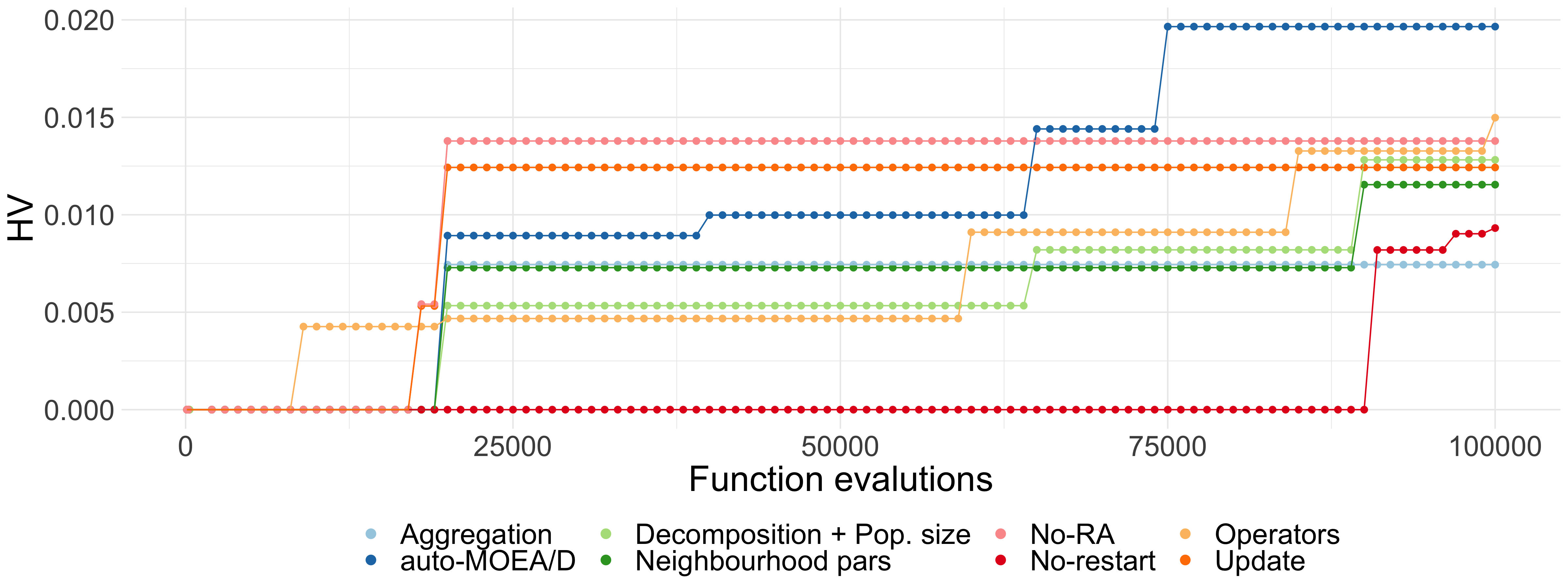
Figure 13. MAZDA - all variants perform badly, with auto-MOEA/D achieving the highest HV value.

Here, we analyse the anytime performance effects in terms of HV values to investigate the impact of different components variants and auto-MOEA/D in analytical and simulated real-world problems. We first start our analysis using the DASCMOP1-3 and 9, Figure 6, as auto-MOEA/D has a very poor performance in the other problems . We can see that for these problems, increments in HV values are followed by periods without changes in performance for almost all of the variants. We can also see that the variants converge before half of the search, except for the update variant in the DASCMOP1-2 problems. For DASCMOP9, the convergence happens a little later, but the HV curves for this problem are overall similar to the other problems.

For the CRE problems, all auto-MOEA/D variants converge at around 25000 evaluations, as we can see in Figures 7, 8, 9, 10 and 11. The exception is for the CRE21 problem, in Figure 7, where not using restart converged to a lower HV value than the other variants. This is similar to the convergence behavior we found for the DASCMOP problems, although the curves here are more balanced. It seems that DASCMOP1-3 and 9 and the CRE problems have little impact on the ability of the auto-MOEA/D variant to perform well in terms of anytime HV performance.

The same observation cannot be made for the MAZDA and MOON problems. We can see in Figures 12 and 13 that most of the variants have trouble improving the HV over the evaluations and that the best variant is problem-dependent. For both problems, increments in HV values are followed by periods without changes in performance for almost all of the variants. This is similar behavior to the DASCMOP problems; however, here we see that the periods without increments are much longer. Interestingly, for the MAZDA problem not-using restart has generally very low performance during almost all of the search progress to only at the very end improving the performance substantially.

7.3. Decision Behavior Dynamics

Based on the results shown above, we compared the auto-MOEA/D and its variants in terms of HV, final population variance, and the STNs metrics: number of nodes, shared nodes and the number of solutions in the best approximation to the Pareto front .. For a more straightforward comparative analysis, we calculate the difference between the results found by the variants to the results found by the auto-MOEA/D (Table 3). We show the $\Delta$HV, $\Delta$nodes, $\Delta$variance . For all of these metrics, positive values indicate larger values in relation to the base algorithm, while negative values indicate the opposite. The number of shared nodes and solutions in the Pareto front are the two absolute metrics.

Table 5. $\Delta$HV; number of $\Delta$nodes; $\Delta$variance of the population, number of Shared nodes and the number of solutions in the Pareto front (#PF) given the different variants of the auto-MOEA/D in terms of components on the constrained problems.

	Decomposition + pop. size variant						Aggregation function variant
MOP	$\Delta$HV	SD	$\Delta$nodes	$\Delta$variance	Shared	#PF	$\Delta$HV	SD	$\Delta$nodes	$\Delta$variance	Shared	#PF
DASCMOP1	-0.001	0	313	-0.012	1	478	0	0.002	-86	0.03	703	424
DASCMOP2	-0.001	0	757	-0.005	3	556	0	0.002	90	0.007	743	611
DASCMOP3	0	0	1884	0.026	3	66	0.003	0.007	59	0.077	790	78
DASCMOP4	-0.116	0.043	103	-1.847	4	0	0	0	-10	-0.291	2141	0
DASCMOP5	0	0.058	183	-1.532	5	0	0.114	0.041	-6	-0.13	2168	0
DASCMOP6	-0.113	0.041	159	-1.138	5	0	0	0	0	-0.112	2140	0
DASCMOP7	0	0	178	-1.315	7	0	0	0	26	0.015	2196	0
DASCMOP8	-0.124	0.391	234	-0.835	7	0	0	0	15	-0.108	2262	0
DASCMOP9	0.126	0.53	3483	0.006	6	12	-0.123	0.024	1162	-0.011	2618	17
MOON	-0.113	0.371	272	-0.076	343	2	0.096	0.451	7	0.004	911	2
MAZDA	0.007	0.02	3682	-4.762	5	0	0.012	0.023	-118	0.144	1790	0
CRE21	-0.007	0.007	1753	0	192	0	-0.001	0.008	22	0.034	4562	0
CRE22	0	0.001	198	0.064	27	19	0	0.001	69	-0.033	551	15
CRE23	0.009	0.004	2862	-0.007	374	3	0.001	0.005	-101	-0.014	1362	2
CRE31	0.01	0.001	1433	-0.01	4	5	0.004	0.004	439	0.048	556	7
CRE32	0.003	0.002	6693	0.025	17	0	0.01	0.019	339	0.109	1267	0
	Update variant						Neighbourhood parameter variant
DASCMOP1	0.774	0.569	954	-0.145	258	284	0	0.002	-67	0.033	214	408
DASCMOP2	0.925	0.508	-175	-0.035	267	385	0	0.002	-31	-0.009	222	559
DASCMOP3	-0.004	0.015	1338	-0.038	328	73	0.001	0.007	423	0.005	263	87
DASCMOP4	0	0	-1786	0.277	410	0	0	0	127	1.398	212	0
DASCMOP5	0.114	0.041	-1793	0.358	403	0	0.114	0.041	120	1.148	214	0
DASCMOP6	0	0	-1777	0.411	402	0	0	0	111	1.576	211	0
DASCMOP7	0	0	-1908	1.812	420	0	0	0	-69	0.993	229	0
DASCMOP8	0	0	-1890	-0.364	448	0	0	0	2	-0.82	246	0
DASCMOP9	-0.023	0.407	3208	-0.208	363	13	-0.128	0.051	366	0.035	268	21
MOON	0.123	0.043	-233	0.002	875	2	-0.103	0.432	-16	-0.03	743	2
MAZDA	0.007	0.026	1107	0.367	230	0	0.008	0.025	-149	-0.472	209	0
CRE21	0.002	0.009	-3306	-0.005	797	0	0.007	0.014	-314	0	860	0
CRE22	0	0.001	158	0.028	445	14	0	0	85	0.064	380	17
CRE23	0.005	0.009	969	0.013	1598	1	0.001	0.005	249	-0.013	1299	1
CRE31	-0.001	0.003	224	0	444	7	0.002	0.002	164	-0.038	414	8
CRE32	0.011	0.031	2767	0.033	745	0	-0.003	0.013	950	0.076	607	0
	Operators variant						No-restart variant
DASCMOP1	0.001	0.002	1389	-0.109	216	461	0.226	0.474	3739	0.038	427	276
DASCMOP2	-0.001	0.002	1129	0.004	223	789	0.004	0.003	3893	0.004	416	356
DASCMOP3	0.005	0.005	41278	0.07	266	79	0.007	0.004	4804	0.043	782	54
DASCMOP4	-0.357	0.574	-361	1.549	215	0	-0.233	0.490	2142	0.352	168	0
DASCMOP5	-0.245	0.578	-291	1.488	217	0	0	0.363	2170	0.947	174	0
DASCMOP6	-0.36	0.58	-273	1.09	215	0	0	0	2134	1.032	172	0
DASCMOP7	-0.656	0.691	-471	1.454	220	0	-0.124	0.392	2241	0.345	135	0
DASCMOP8	-0.787	0.668	-537	0.311	234	0	-0.122	0.384	2304	-0.068	143	0
DASCMOP9	-0.126	0.013	1618	0.048	266	16	-0.014	0.402	11593	-0.124	2202	18
MOON	-0.163	0.364	135	-0.026	727	2	0.307	0.379	1267	-0.011	108	2
MAZDA	0.005	0.024	-1323	1.288	237	0	0.01	0.029	1113	-0.709	906	4
CRE21	0.017	0.040	643	0.054	787	0	0.27	0.423	4318	0.051	416	0
CRE22	0	0	96	0.053	393	17	0	0.001	1849	0.079	157	14
CRE23	0	0.002	-2440	0.002	1478	1	-0.053	0.003	3186	0.005	1336	1
CRE31	-0.002	0.001	-22	0.001	447	8	-0.002	0.004	3546	-0.038	619	2
CRE32	0	0.012	850	-0.002	665	0	-0.003	0.016	7569	0.006	2310	0
	No-RA variant
DASCMOP1	0	0.002	-37	-0.061	13	449
DASCMOP2	-0.001	0.002	240	0.005	12	537
DASCMOP3	0.005	0.006	-75	0.012	15	70
DASCMOP4	0	0	-108	0.586	11	0
DASCMOP5	0.114	0.041	-45	-0.014	13	0
DASCMOP6	0	0	-97	0.018	12	0
DASCMOP7	-0.121	0.381	-58	0.51	14	0
DASCMOP8	-0.118	0.374	-49	-0.52	15	0
DASCMOP9	0.008	0.395	493	-0.093	12	14
MOON	-0.052	0.406	-14	-0.052	417	2
MAZDA	0.006	0.03	-141	0.435	12	0
CRE21	0.004	0.01	78	0.065	550	0
CRE22	0	0	-55	0.053	35	24
CRE23	-0.013	0.002	-286	-0.013	622	2
CRE31	-0.001	0.002	53	-0.004	24	8
CRE32	-0.002	0.017	1 36	-0.001	39	0

The different metrics for the variants are shown in Table 5. Given that we already discussed the HV values above, we focus here on the other metrics shown in this Table.

For the DASCMOP problems, all auto-MOEA/D variants find solutions in the Pareto front, suggesting that reaching the theoretical Pareto front of these problems is not a challenge. The update and the operators variants generally have a lower number of nodes and final population variance. Interestingly the aggregation function variant seems to have little effect in most of the metrics, and we highlight that the number of shared nodes is one or two orders of magnitude higher than the other variants for the DASCMOP3-9. Changing the decomposition method and the population size leads to more differences in areas of the decision space explored but doesn’t affect much the overall HV performance. The same is true for the no-RA variant. This indicates that changing how MOEA/D works with the population during the search can affect how the decision space is explored but doesn’t correspond to increments in HV performance for these problems.

However, for the simulated and analytical real-world problems, we can observe little similarities among the five problems analyzed. This suggests that, unlike the DASCMOP set, the features of each of the simulated and analytical problems impact the auto-MOEA/D differently. For the MOON problem, we can see that the no-restart variant explored fewer areas of decision space, as we can see by the higher difference in the number of nodes. The number of shared nodes is the lowest among all variants, which suggests that auto-MOEA/D and the no-restart variant visit different areas of the decision space. That said, this variant was still able to find solutions in the approximated Pareto front. This suggests that the initial population has a high impact on the search exploration and all methods can follow a path to optimal solutions. We understand that this problem could be seen as a multimodal problem with at least one funnel to optimal solutions; however, more work needs to be done to validate this.

Now, moving to the results of the MAZDA problem. For this problem, the variant that leads to less number of shared nodes, with only 5, the highest number of nodes and the highest final population variance is the decomposition+pop. size variant. This indicates that this variant can visit more areas of the decision space that are not explored by auto-MOEA/D while also having the final population spread to many different areas (given the higher variance). This could mean that choosing the right decomposition method and population size is critical for this problem. To our surprise, this is the only problem where no-restart leads to a noteworthy amount of solutions in the approximation to the Pareto front. Overall, these results show that these problems might have a set of unique characteristics in comparison to the other problems studied here.

Finally, the results of the CRE problems show that in terms of the number of nodes the no-restart variant is the one that has the biggest differences, exploring less the decision space and that not using RA was able to increase the number of solutions in the approximation to the Pareto front, with little differences in the other metrics. That is, the aggregation function has generally the highest number of shared solutions in the two sets of problems and the no-restart variant has about the same difference in terms of the number of nodes. This is in agreement with Table 3. Thus we believe that DASCMOP1-3 and 9 might share similar problems characteristics with the CRE problem set.

7.4. STNs Extension for Pairs of MOEAs

For creating merged STN models of pairs of MOEAs, we first need to create one STN for each algorithm. To create the STN of a single algorithm, we follow a recently proposed methodology (Lavinas et al., 2022a, c).

As discussed (Section 3), we extend this approach by merging the trajectories of two of these STNs by joining the two STNs graphs. This merged STN model contains the nodes and edges present in the STN of at least one algorithm. Attributes are kept for the nodes and edges, indicating whether they were visited by both algorithms (shared) or by one of them only.

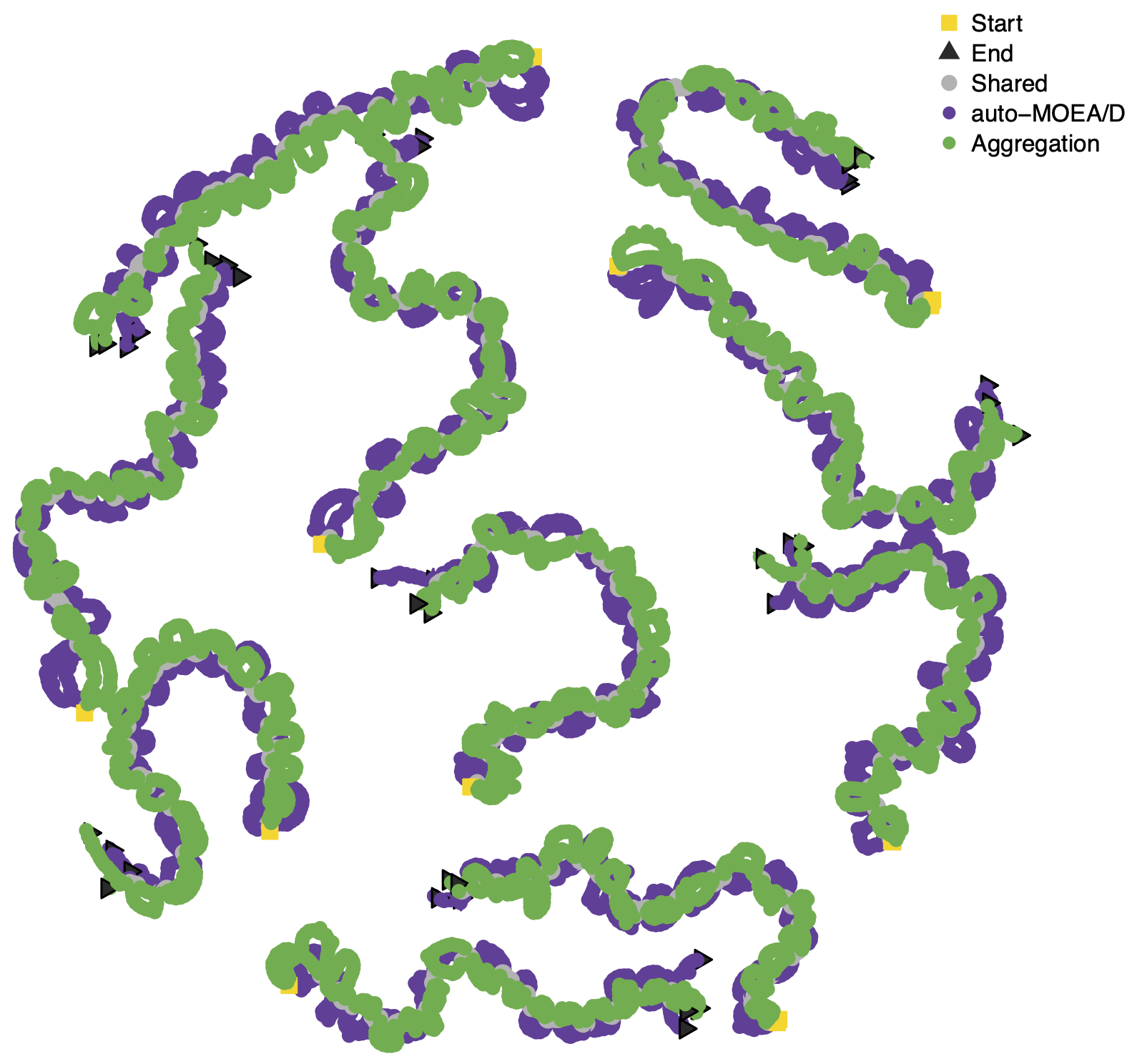
((a)) DASCMOP1

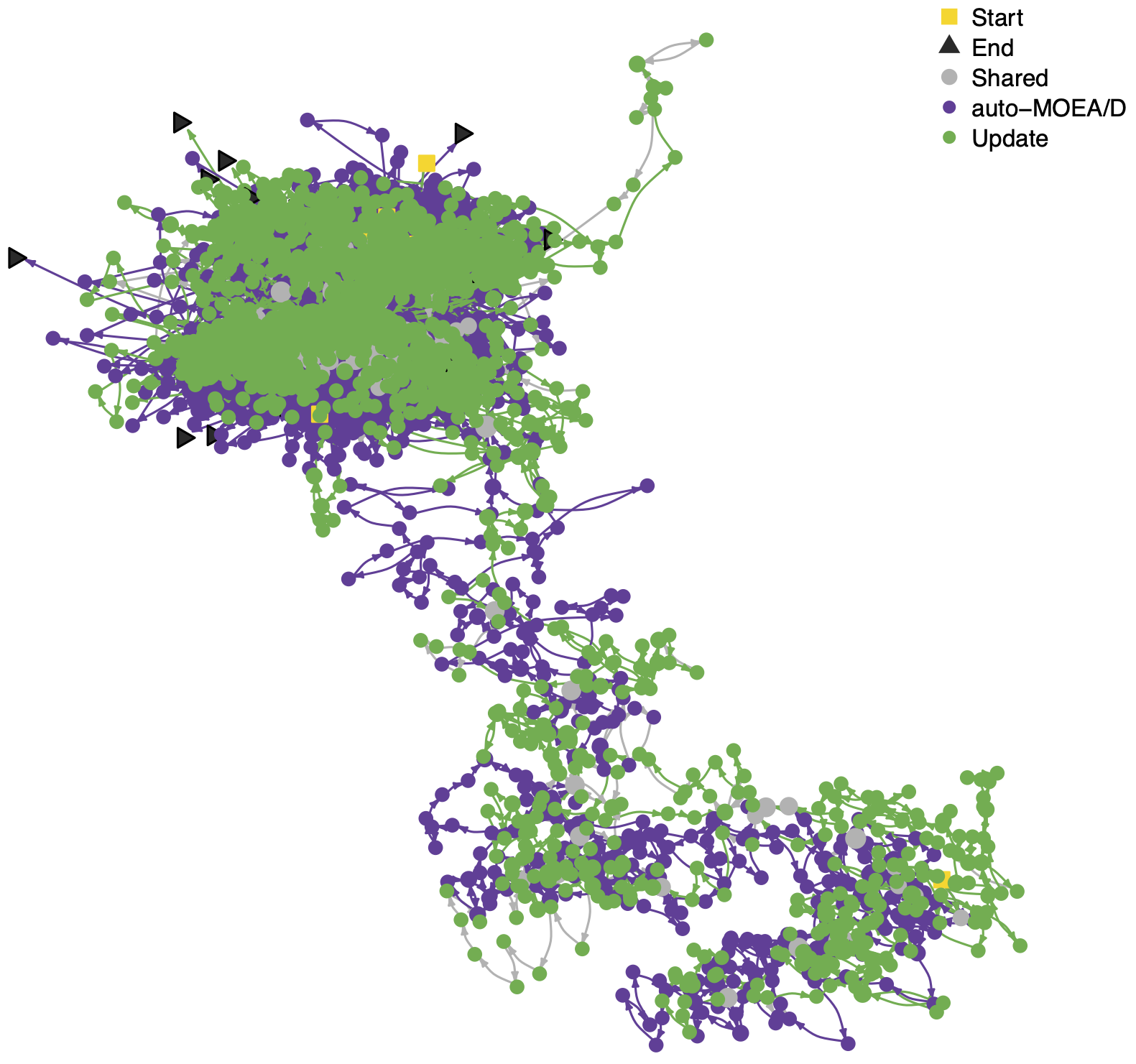
((b)) DASCMOP2

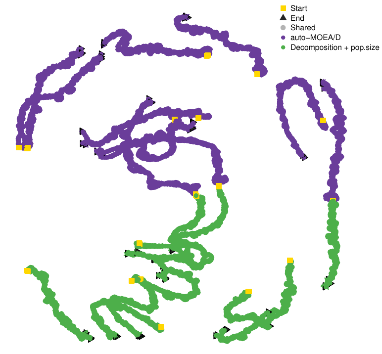
((c)) DASCMOP3

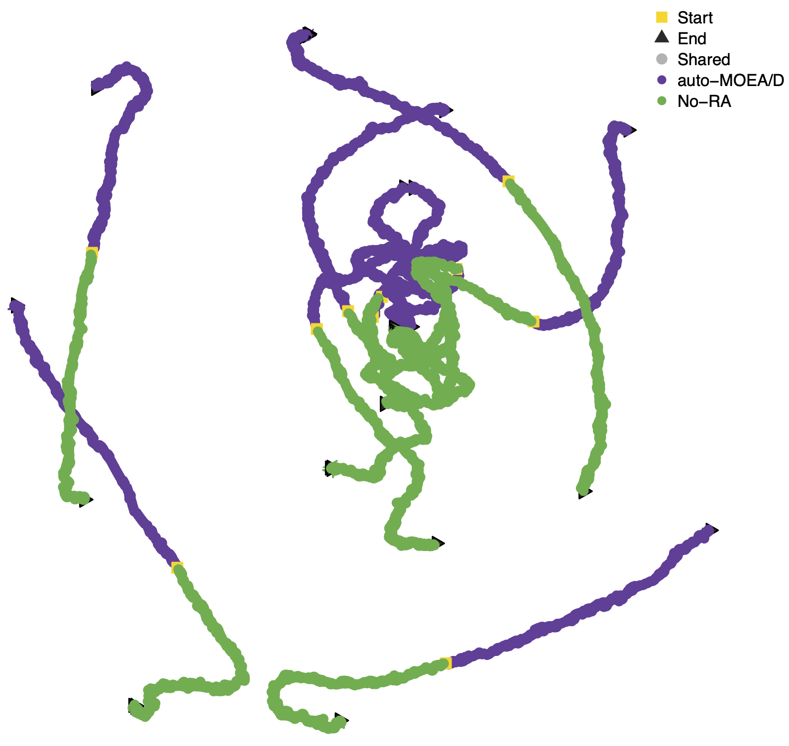
((d)) DASCMOP4

Figure 14. STN of auto-MOEA/D and different variants on the easy DASCMOP group. We see a diverse set of behaviors, from interlinked trajectories on the upper side to trajectories that visit distinct regions of the decision space on the bottom side.

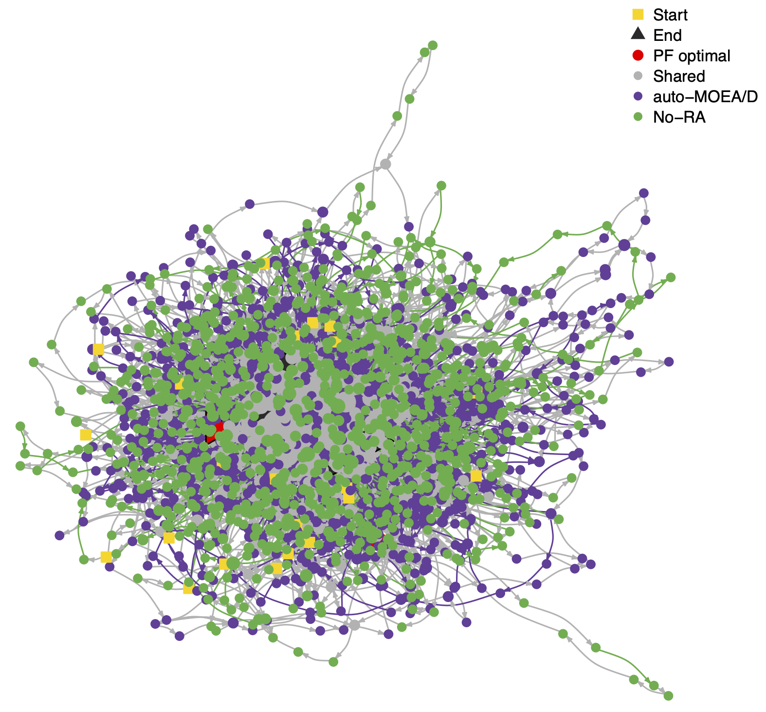
((a)) The trajectories of auto-MOEA/D and the no-RA variant overlap and share multiple locations, as shown by the grey nodes.

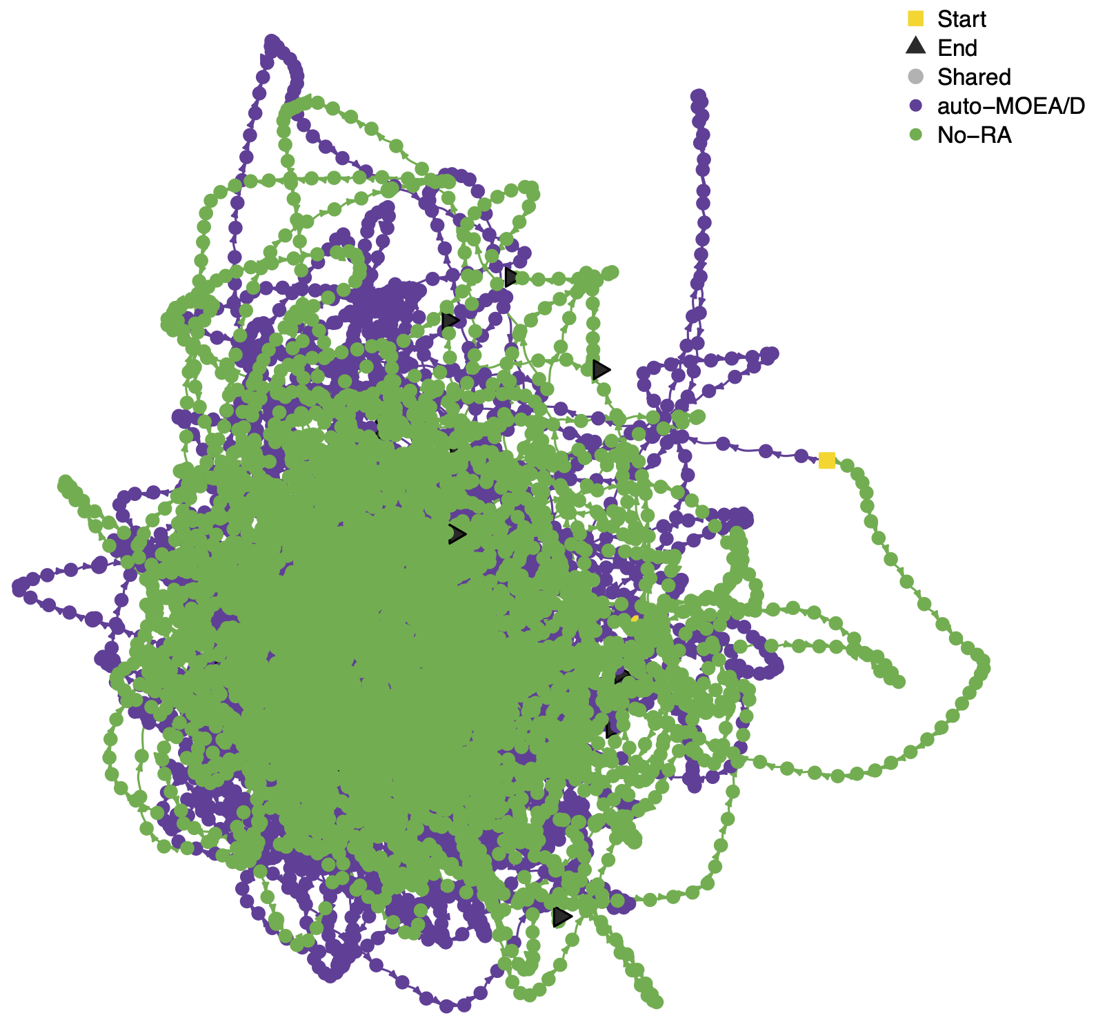
((b)) The trajectories of auto-MOEA/D and the no-RA variant share few locations (not visible).

Figure 15. STNs of auto-MOEA/D and two variants on the MOON (left) and MAZDA (right) problems. The MAZDA problem has a bigger effects the trajectories of the variants.

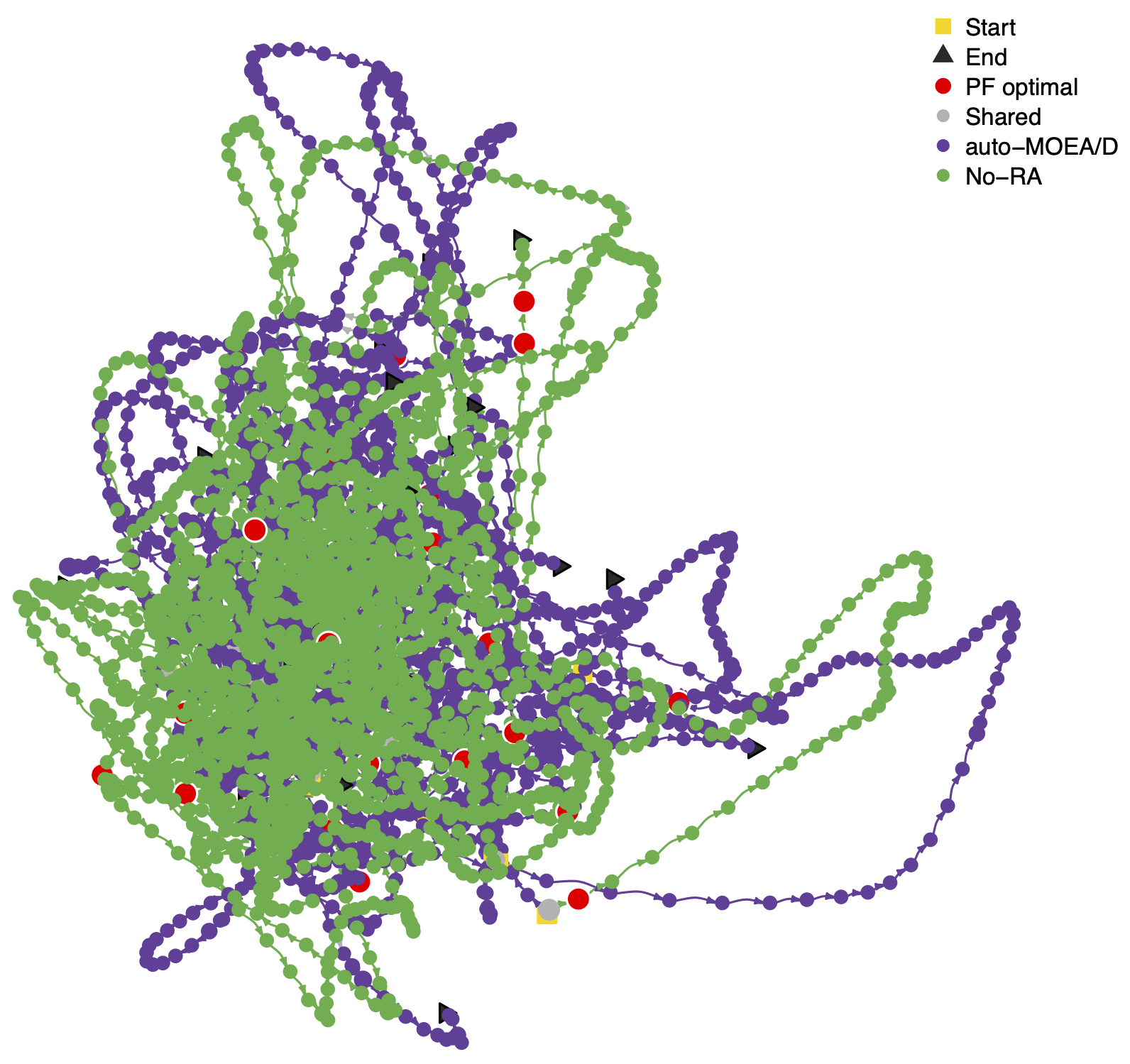
((a)) The trajectories of auto-MOEA/D and the no-RA variant visit many optimal solutions.

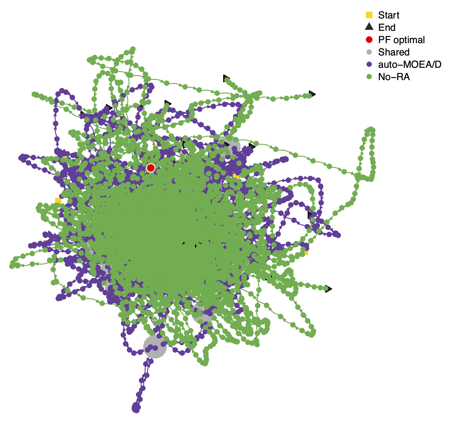
((b)) The trajectories of auto-MOEA/D and the no-RA variant visit few optimal solutions.

Figure 16. STNs of auto-MOEA/D and two variants on the CRE22 (left) and CRE23 (right) problems. The variants reach the approximation to the Pareto front.

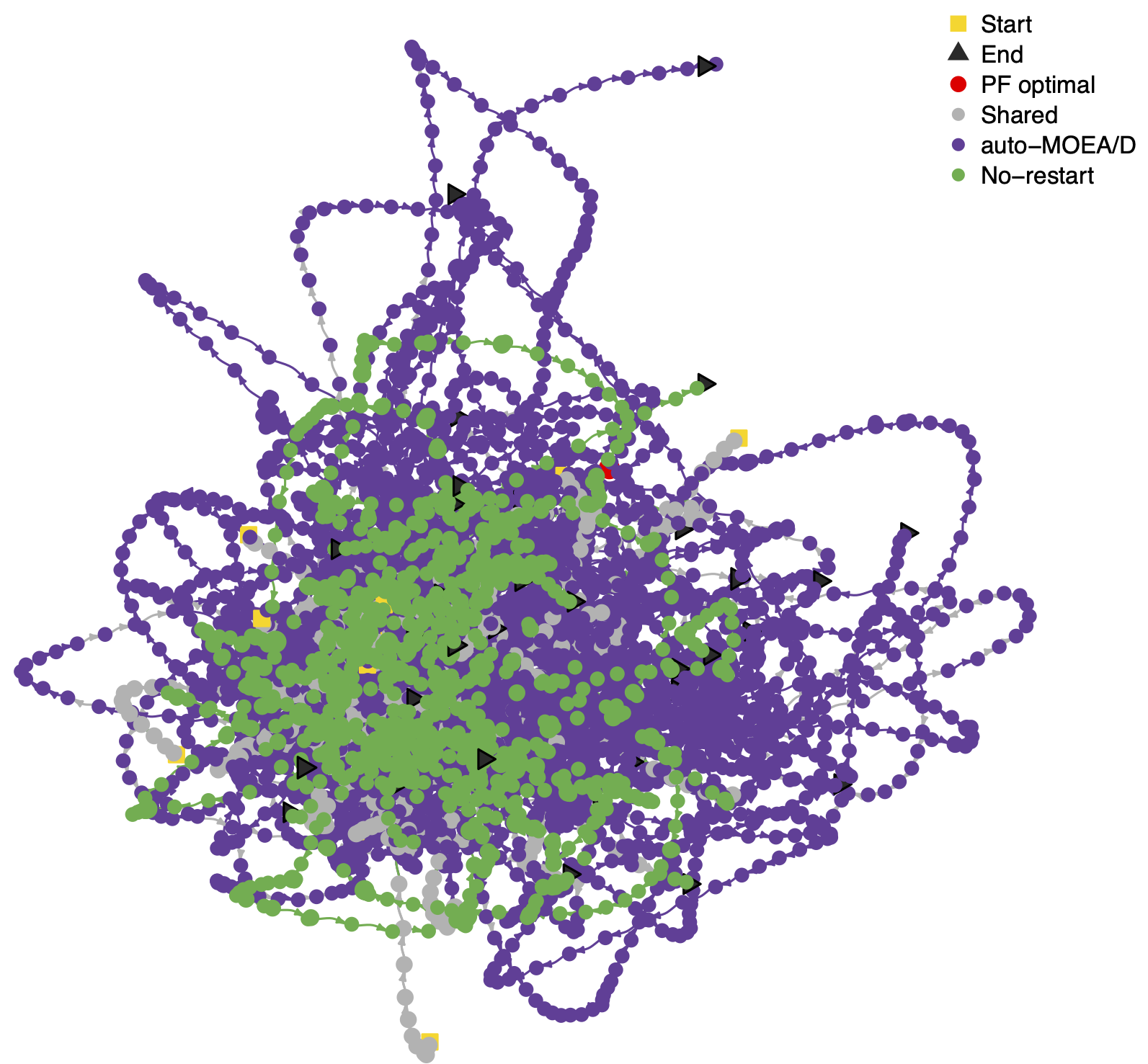
((a)) The trajectories of auto-MOEA/D and the operators variant are similar.

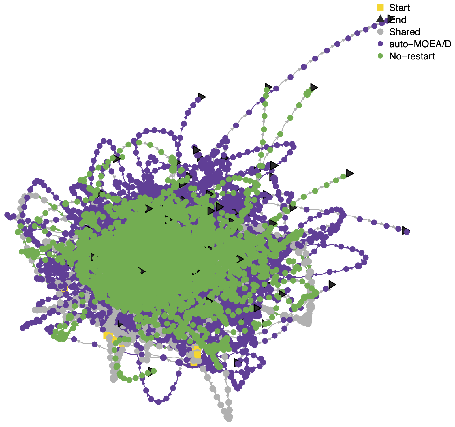
((b)) The trajectories of auto-MOEA/D and the no-restart variant share some nodes.

Figure 17. STNs of auto-MOEA/D and the two variants on the CRE31 (left) and CRE22 (right) problem.

Moving on to the STNs visualisations, Figures 14, 15,  16 and  17. We selected visualisations of a representative variant for each problem. Considering the colours used in the STN visualisations, yellow squares indicate the start of trajectories, and black triangles indicate the end of trajectories. The red colour shows the Pareto optimal solutions, and light grey circles show shared locations visited by both algorithms in that MOP. Finally, the trajectories of each algorithm are shown in different colours: purple for the auto-MOEA/D and green for the variant.

First of all, we comment on the overall differences among the STNs of the DASCMOP problems, Figure 14, and the simulated and analytical real-world problems  15,  16 and  17. Unlikely the anytime HV performance that showed a similar objective space behavior between the DASCMOP and CRE problems, we can see that the decision space behavior of the DASCMOP STNs is more diverse when compared to the behavior of shown by the STNs for the real-world problems. This finding demonstrates how essential it is to explore the decision space behavior of algorithms.

For the simulated MOON and MAZDA problem in Figures 15, we can see that the trajectories are similar, with multiple shared nodes. That is, the trajectories of the STNs of the auto-MOEA/D and each variant overlap, visiting similar regions in the decision space. We associate this behavior with the number of shared nodes for this problem being high for all variants. Although we only showed the STNs of one pair, an identical trend occurs for all pairs of the auto-MOEA/D variants for the MOON problem. We understand this is indicative that the features of this simulated problem affect all MOEAs studied here in a similar fashion. The opposite happens for the MAZDA problem, where the trajectories shown in the Figure visit unrelated areas of the decision space. For the pair selected, the trajectories do not overlap, and the number of shared nodes is much smaller. However, we can see in Table 5 that there is no agreement among the different variants in the metrics indicating a high impact of the problem difficulty on the search behavior of the different variants exploring the problem differently.

Moving now to the analytical CRE problems in Figures 16 and  17. We highlight that the trajectories of all variants for these problems overlap each other. Thus, we understand that the auto-MOEA/D variants visit similar regions in the decision space. Although the number of shared nodes is high for most of the variants in these problems, we can see that the variants are affected differently given the problem in question, indicating a contrasting set of features among the problems. In terms of best Pareto optimal solutions, we can see that there are much more solutions in the approximation to the Pareto front for the CRE22 problem than for the CRE23. We can see in Table 5 that an identical trend occurs for all pairs of the auto-MOEA/D variants for both problems. For the three objective problems, CRE31 and CRE32 we can see that the number of Pareto optimal solutions reduce substantially.

8. Conclusion

This works defines a new methodology to investigate the effects of algorithmic components based on our previous work (Lavinas et al., 2022c) that takes into account the decision space dynamics, as well as the objective space dynamics of the components. This methodology allows the user to investigate the impacts of the components of multiobjective algorithms in analytical and simulated problems with constraints. We contrasted the behavior of these configurations in terms of how they explore the decision space by comparing their Search Trajectory Networks (STNs), their population diversity, and how they behave in the objective space by exploring the anytime performance effects in terms of HV values. This analysis allowed us to identify the most influential components in the different problems we studied here.

Interestingly, the results shown in this paper differ from the ones found on our previous work. This is mainly because the training method used in the original paper was using a set of constraints that were too hard for MOEA/D to deal with. Since we wanted to improve the overall quality of the tuned MOEA/D in the hard set of problems we used a set of constraint difficulty triples of the DASCMOP benchmark set. That lead to increments in the performance of the tuned MOEA/D in the problems it was already performing well, but not affecting the performance in problems it had difficulties with. Thus, we understand that the results and conclusions are not accidental, but dependent on the different algorithm configuration selected.

We applied this methodology the auto-MOEA/D, a tuned MOEA/D designed by the irace package, and the subsequently derived variants that differ from this machine-designed MOEA by a single component. Our results showed that the most potentially influential variants differ given the set of problems: (1) for the DASCMOP problems the update variant showed more different behaviors in the objective and decision spaces; (2) the no-restart variant was more affected by the features of MOON problem while the decomposition+pop. size variant was the one that was more affected by the features of the MAZDA problem and (3) for the CRE family the variants that caused more changes in the decision space exploration behavior are the aggregation function and the no-restart. However, it is still necessary to establish the generalization of such results ans how can we extrapolate to characterize the behavior of components independently of the scenarios observed.

We found that analysing the objective and the decision space simultaneously provides complementary information about how algorithms behave as the search progresses. In addition, the decision space behavior analysis was able to slightly contribute to the characterization of problems. For example, given how the trajectories of the STNs of the auto-MOEA/D and each other variant for the MOON problem frequently overlap, thus this problem could be seen as a multimodal problem with at least one funnel to optimal solutions; but, more work needs to be done to validate this. Moreover, this finding demonstrates how essential it is to explore the decision space behavior of algorithms.

In summary, this study strengthens the view that characterizing the effects of MOEA/D algorithm components could help in developing even more effective MOEAs. Taken together, these findings suggest a role for improving in promoting the study of specific components to develop new and better components. We understand that our results are of interest to the broad multiobjective evolutionary computation community.

One limitation of this methodology is that the search space of possible algorithm configurations is limited by the choices of components and components parameters. However, with a careful selection of those, automatic composition can be a powerful tool to explore this possibility space.

References

- (1)
- Aguirre et al. (2014) Hernán Aguirre, Arnaud Liefooghe, Sébastien Verel, and Kiyoshi Tanaka. 2014. An Analysis on Selection for High-Resolution Approximations in Many-Objective Optimization. In Parallel Problem Solving from Nature – PPSN XIII, Thomas Bartz-Beielstein, Jürgen Branke, Bogdan Filipič, and Jim Smith (Eds.). Springer International Publishing, Cham, 487–497.
- Aguirre and Tanaka (2007) Hernán E. Aguirre and Kiyoshi Tanaka. 2007. Working principles, behavior, and performance of MOEAs on MNK-landscapes. European Journal of Operational Research 181, 3 (2007), 1670–1690. https://doi.org/10.1016/j.ejor.2006.08.004
- Beume et al. (2007) Nicola Beume, Boris Naujoks, and Michael Emmerich. 2007. SMS-EMOA: Multiobjective selection based on dominated hypervolume. European Journal of Operational Research 181, 3 (2007), 1653–1669.
- Bezerra et al. (2015a) Leonardo CT Bezerra, Manuel López-Ibáñez, and Thomas Stützle. 2015a. Comparing decomposition-based and automatically component-wise designed multi-objective evolutionary algorithms. In International Conference on Evolutionary Multi-Criterion Optimization. Springer, 396–410.
- Bezerra et al. (2019) Leonardo C. T. Bezerra, Manuel López-Ibáñez, and Thomas Stützle. 2019. Archiver Effects on the Performance of State-of-the-Art Multi- and Many-Objective Evolutionary Algorithms. In Proceedings of the Genetic and Evolutionary Computation Conference (Prague, Czech Republic) (GECCO ’19). Association for Computing Machinery, New York, NY, USA, 620–628. https://doi.org/10.1145/3321707.3321789
- Bezerra et al. (2015b) Leonardo C. T. Bezerra, Manuel López-Ibáñez, and Thomas Stützle. 2015b. Comparing Decomposition-Based and Automatically Component-Wise Designed Multi-Objective Evolutionary Algorithms. In Evolutionary Multi-Criterion Optimization, António Gaspar-Cunha, Carlos Henggeler Antunes, and Carlos Coello Coello (Eds.). Springer International Publishing, Cham, 396–410.
- Bezerra et al. (2020a) Leonardo C. T. Bezerra, Manuel López-Ibáñez, and Thomas Stützle. 2020a. Automatic Configuration of Multi-objective Optimizers and Multi-objective Configuration. Springer International Publishing, Cham, 69–92. https://doi.org/10.1007/978-3-030-18764-4˙4
- Bezerra et al. (2020b) Leonardo C. T. Bezerra, Manuel López-Ibáñez, and Thomas Stützle. 2020b. Automatically Designing State-of-the-Art Multi- and Many-Objective Evolutionary Algorithms. Evolutionary Computation 28, 2 (2020), 195–226. https://doi.org/10.1162/evco˙a˙00263
- Bezerra et al. (2016) Leonardo C. T. Bezerra, Manuel López-Ibáñez, and Thomas Stützle. 2016. Automatic Component-Wise Design of Multiobjective Evolutionary Algorithms. IEEE Transactions on Evolutionary Computation 20, 3 (2016), 403–417. https://doi.org/10.1109/TEVC.2015.2474158
- Blank and Deb (2020) J. Blank and K. Deb. 2020. pymoo: Multi-Objective Optimization in Python. IEEE Access 8 (2020), 89497–89509.
- Campelo and Aranha (2018) Felipe Campelo and Claus Aranha. 2018. MOEADr: Component-Wise MOEA/D Implementation. URL https://cran.R-project.org/package=MOEADr. R package version 1.2.0.
- Campelo et al. (2020) Felipe Campelo, Lucas Batista, and Claus Aranha. 2020. The MOEADr Package: A Component-Based Framework for Multiobjective Evolutionary Algorithms Based on Decomposition. Journal of Statistical Software (2020). In press. Available from: https://arxiv.org/abs/1807.06731.
- Csardi and Nepusz (2006) G. Csardi and T. Nepusz. 2006. The igraph software package for complex network research. InterJournal Complex Systems (2006), 1695.
- Deb et al. (2002) Kalyanmoy Deb, Amrit Pratap, Sameer Agarwal, and TAMT Meyarivan. 2002. A fast and elitist multiobjective genetic algorithm: NSGA-II. IEEE transactions on evolutionary computation 6, 2 (2002), 182–197.
- Dubois-Lacoste et al. (2015) Jérémie Dubois-Lacoste, Manuel López-Ibáñez, and Thomas Stützle. 2015. Anytime Pareto local search. European Journal of Operational Research 243, 2 (2015), 369 – 385. https://doi.org/10.1016/j.ejor.2014.10.062
- Eiben and Schippers (1998) A. E. Eiben and C. A. Schippers. 1998. On Evolutionary Exploration and Exploitation. Fundamenta Informaticae 35, 1-4 (Aug. 1998), 35–50.
- Fan et al. (2020) Zhun Fan, Wenji Li, Xinye Cai, Hui Li, Caimin Wei, Qingfu Zhang, Kalyanmoy Deb, and Erik Goodman. 2020. Difficulty Adjustable and Scalable Constrained Multiobjective Test Problem Toolkit. Evolutionary Computation 28, 3 (09 2020), 339–378. https://doi.org/10.1162/evco˙a˙00259 arXiv:https://direct.mit.edu/evco/article-pdf/28/3/339/1858953/evco_a_00259.pdf
- Fawcett and Hoos (2016) Chris Fawcett and Holger H Hoos. 2016. Analysing differences between algorithm configurations through ablation. Journal of Heuristics 22, 4 (2016), 431–458.
- Fieldsend and Alyahya (2019) Jonathan E. Fieldsend and Khulood Alyahya. 2019. Visualising the Landscape of Multi-Objective Problems Using Local Optima Networks. In Proceedings of the Genetic and Evolutionary Computation Conference Companion (Prague, Czech Republic) (GECCO ’19). Association for Computing Machinery, New York, NY, USA, 1421–1429. https://doi.org/10.1145/3319619.3326838
- Fonseca and Fleming (1996a) Carlos M Fonseca and Peter J Fleming. 1996a. On the performance assessment and comparison of stochastic multiobjective optimizers. In International Conference on Parallel Problem Solving from Nature. Springer, 584–593.
- Fonseca and Fleming (1996b) Carlos M. Fonseca and Peter J. Fleming. 1996b. On the performance assessment and comparison of stochastic multiobjective optimizers. In Parallel Problem Solving from Nature — PPSN IV, Hans-Michael Voigt, Werner Ebeling, Ingo Rechenberg, and Hans-Paul Schwefel (Eds.). Springer Berlin Heidelberg, Berlin, Heidelberg, 584–593.
- Hifi et al. (2021) Mhand Hifi, Hugo Monzón Maldonado, Hernán Aguirre, Sébastien Verel, Arnaud Liefooghe, Bilel Derbel, and Kiyoshi Tanaka. 2021. Understanding Population Dynamics in Multi- and Many-Objective Evolutionary Algorithms for High-Resolution Approximations. Advances in Operations Research 2021 (2021), 6699277. https://doi.org/10.1155/2021/6699277
- Joines and Houck (1994) J.A. Joines and C.R. Houck. 1994. On the use of non-stationary penalty functions to solve nonlinear constrained optimization problems with GA’s. In Proceedings of the First IEEE Conference on Evolutionary Computation. IEEE World Congress on Computational Intelligence. 579–584 vol.2. https://doi.org/10.1109/ICEC.1994.349995
- Joshi and Deshpande (2014) Ramprasad Joshi and Bharat Deshpande. 2014. Empirical and analytical study of many-objective optimization problems: analysing distribution of nondominated solutions and population size for scalability of randomized heuristics. Memetic Computing 6, 2 (2014), 133–145.
- Kerschke and Grimme (2017) Pascal Kerschke and Christian Grimme. 2017. An Expedition to Multimodal Multi-objective Optimization Landscapes. In Evolutionary Multi-Criterion Optimization, EMO (Lecture Notes in Computer Science, Vol. 10173). Springer, 329–343. https://doi.org/10.1007/978-3-319-54157-0_23
- Kohira et al. (2018) Takehisa Kohira, Hiromasa Kemmotsu, Oyama Akira, and Tomoaki Tatsukawa. 2018. Proposal of benchmark problem based on real-world car structure design optimization. In Proceedings of the Genetic and Evolutionary Computation Conference Companion. ACM, 183–184.
- Lavinas et al. (2020) Yuri Lavinas, Claus Aranha, Marcelo Ladeira, and Felipe Campelo. 2020. MOEA/D with Random Partial Update Strategy. In 2020 IEEE Congress on Evolutionary Computation (CEC). 1–8.
- Lavinas et al. (2022a) Yuri Lavinas, Claus Aranha, and Gabriela Ochoa. 2022a. Search Trajectories Networks of Multi-objective Evolutionary Algorithms”. In International Conference on the Applications of Evolutionary Computation (Part of EvoStar). Springer, to appear.
- Lavinas et al. (2022b) Yuri Lavinas, Marcelo Ladeira, and Claus Aranha. 2022b. Faster Convergence in Multi-Objective Optimization Algorithms Based on Decomposition. Evolutionary Computation (02 2022), 1–26. https://doi.org/10.1162/evco˙a˙00306
- Lavinas et al. (2022c) Yuri Lavinas, Marcelo Ladeira, Gabriela Ochoa, and Claus Aranha. 2022c. Component-Wise Analysis of Automatically Designed Multiobjective Algorithms on Constrained Problems. In Proceedings of the Genetic and Evolutionary Computation Conference (Boston, Massachusetts) (GECCO ’22). Association for Computing Machinery, New York, NY, USA, 538–546. https://doi.org/10.1145/3512290.3528719
- Li and Zhang (2009) Hui Li and Qingfu Zhang. 2009. Multiobjective Optimization Problems With Complicated Pareto Sets, MOEA/D and NSGA-II. IEEE Transactions on Evolutionary Computation 13, 2 (2009), 284–302. https://doi.org/10.1109/TEVC.2008.925798
- Liefooghe et al. (2018) Arnaud Liefooghe, Bilel Derbel, Sébastien Verel, Manuel López-Ibáñez, Hernán Aguirre, and Kiyoshi Tanaka. 2018. On Pareto Local Optimal Solutions Networks. In Parallel Problem Solving from Nature – PPSN XV, Anne Auger, Carlos M. Fonseca, Nuno Lourenço, Penousal Machado, Luís Paquete, and Darrell Whitley (Eds.). Springer International Publishing, Cham, 232–244.
- López-Ibáñez et al. (2016) Manuel López-Ibáñez, Jérémie Dubois-Lacoste, Leslie Pérez Cáceres, Mauro Birattari, and Thomas Stützle. 2016. The irace package: Iterated racing for automatic algorithm configuration. Operations Research Perspectives 3 (2016), 43–58. https://doi.org/10.1016/j.orp.2016.09.002
- Nebro et al. (2019) Antonio J. Nebro, Manuel López-Ibáñez, Cristóbal Barba-González, and José García-Nieto. 2019. Automatic Configuration of NSGA-II with JMetal and Irace. In Proceedings of the Genetic and Evolutionary Computation Conference Companion (Prague, Czech Republic) (GECCO ’19). Association for Computing Machinery, New York, NY, USA, 1374–1381. https://doi.org/10.1145/3319619.3326832
- Nishiyama et al. (2015) Mari Nishiyama, Hisashi Otake, Takeshi Hoshino, Tatsuaki Hashimoto, Takeshi Watanabe Watanabe, Tomoaki Tatsuaki, and Akira Oyama. 2015. Selection of Landing Sites for Lunar Lander with “KAGUYA” Data Using Multi-Objective Optimization (In Japanese with English abstract). In Space Science Informatics Symposium FY2014.
- Ochoa et al. (2020) Gabriela Ochoa, Katherine M. Malan, and Christian Blum. 2020. Search Trajectory Networks of Population-Based Algorithms in Continuous Spaces. In Applications of Evolutionary Computation, Pedro A. Castillo, Juan Luis Jiménez Laredo, and Francisco Fernández de Vega (Eds.). Springer International Publishing, Cham, 70–85.
- Ochoa et al. (2021) Gabriela Ochoa, Katherine M. Malan, and Christian Blum. 2021. Search trajectory networks: A tool for analysing and visualising the behaviour of metaheuristics. Applied Soft Computing 109 (2021), 107492. https://doi.org/10.1016/j.asoc.2021.107492
- Radulescu et al. (2013a) Andreea Radulescu, Manuel López-Ibáñez, and Thomas Stützle. 2013a. Automatically Improving the Anytime Behaviour of Multiobjective Evolutionary Algorithms. In Evolutionary Multi-Criterion Optimization, Robin C. Purshouse, Peter J. Fleming, Carlos M. Fonseca, Salvatore Greco, and Jane Shaw (Eds.). Springer Berlin Heidelberg, Berlin, Heidelberg, 825–840.
- Radulescu et al. (2013b) Andreea Radulescu, Manuel López-Ibáñez, and Thomas Stützle. 2013b. Automatically Improving the Anytime Behaviour of Multiobjective Evolutionary Algorithms. In Evolutionary Multi-Criterion Optimization, Robin C. Purshouse, Peter J. Fleming, Carlos M. Fonseca, Salvatore Greco, and Jane Shaw (Eds.). Springer Berlin Heidelberg, Berlin, Heidelberg, 825–840.
- Schäpermeier et al. (2020) Lennart Schäpermeier, Christian Grimme, and Pascal Kerschke. 2020. One PLOT to Show Them All: Visualization of Efficient Sets in Multi-objective Landscapes. In Parallel Problem Solving from Nature – PPSN XVI, Thomas Bäck, Mike Preuss, André Deutz, Hao Wang, Carola Doerr, Michael Emmerich, and Heike Trautmann (Eds.). Springer International Publishing, Cham, 154–167.
- Tanabe and Ishibuchi (2020) Ryoji Tanabe and Hisao Ishibuchi. 2020. An easy-to-use real-world multi-objective optimization problem suite. Applied Soft Computing 89 (2020), 106078. https://doi.org/10.1016/j.asoc.2020.106078
- Tanabe et al. (2017) Ryoji Tanabe, Hisao Ishibuchi, and Akira Oyama. 2017. Benchmarking multi-and many-objective evolutionary algorithms under two optimization scenarios. IEEE Access 5 (2017), 19597–19619.
- Vaz et al. (2021) Felipe Vaz, Yuri Lavinas, Claus Aranha, and Marcelo Ladeira. 2021. Exploring Constraint Handling Techniques in Real-World Problems on MOEA/D with Limited Budget of Evaluations. In Evolutionary Multi-Criterion Optimization, Hisao Ishibuchi, Qingfu Zhang, Ran Cheng, Ke Li, Hui Li, Handing Wang, and Aimin Zhou (Eds.). Springer International Publishing, Cham, 555–566.
- Zapotecas-Martínez et al. (2015) Saul Zapotecas-Martínez, Hernán Aguirre, Kiyoshi Tanaka, and Carlos Coello. 2015. On the Low-Discrepancy Sequences and Their Use in MOEA/D for High-Dimensional Objective Spaces. In Congress on Evol. Computation (CEC 2015). 2835–2842.
- Zhang and Li (2007) Qingfu Zhang and Hui Li. 2007. MOEA/D: A Multiobjective Evolutionary Algorithm Based on Decomposition. IEEE Transactions on Evolutionary Computation 11, 6 (2007), 712–731. https://doi.org/10.1109/TEVC.2007.892759
- Zilberstein (1996) Shlomo Zilberstein. 1996. Using anytime algorithms in intelligent systems. AI magazine 17, 3 (1996), 73–73.