Feature Reweighting for EEG-based Motor Imagery Classification

Abstract

Classification of motor imagery (MI) using non-invasive electroencephalographic (EEG) signals is a critical objective as it is used to predict the intention of limb movements of a subject. In recent research, convolutional neural network (CNN) based methods have been widely utilized for MI-EEG classification. The challenges of training neural networks for MI-EEG signals classification include low signal-to-noise ratio, non-stationarity, non-linearity, and high complexity of EEG signals. The features computed by CNN-based networks on the highly noisy MI-EEG signals contain irrelevant information. Subsequently, the feature maps of the CNN-based network computed from the noisy and irrelevant features contain irrelevant information. Thus, many non-contributing features often mislead the neural network training and degrade the classification performance. Hence, a novel feature reweighting approach is proposed to address this issue. The proposed method gives a noise reduction mechanism named feature reweighting module that suppresses irrelevant temporal and channel feature maps. The feature reweighting module of the proposed method generates scores that reweight the feature maps to reduce the impact of irrelevant information. Experimental results show that the proposed method significantly improved the classification of MI-EEG signals of Physionet EEG-MMIDB and BCI Competition IV 2a datasets by a margin of $9.34\%$ and $3.82\%$, respectively, compared to the state-of-the-art methods.

Keywords Electroencephalography (EEG), Brain-computer interfaces (BCIs), motor imagery (MI), convolutional neural network (CNN), and feature reweighting.

1 Introduction

Brain-Computer Interface (BCI) has opened a new dimension for enclosing the proximity between machines and humans. BCI technologies help to establish communication between external devices and the human brain. Electroencephalography (EEG) is a highly preferred type of BCI as it is a high temporal resolution technology with non-invasiveness, cost efficiency, and easy portability characteristics. EEG-based BCI systems include different paradigms, such as P300, steady-state visual evoked potentials (SSVEPs), and motor imagery (MI). Among these, MI has attracted the interest of researchers to a large extent. MI is defined as the spontaneous motor intention/imagination of limb movement (such as hands and legs) without any external stimuli. MI classification corresponds to the identification of the type of spontaneous motor intention/imagery. A wide range of applications of MI includes rehabilitation after motor disabilities [1], smart home applications [2], robotic arm movements [3], complex cursor control [4] and BCI-controlled games [5].

The significant challenges in MI-EEG signal classification are non-linearity, non-stationarity, high complexity, and low signal-to-noise ratio (SNR) of EEG signals [6]. The other challenges are physiological artifacts introduced during EEG acquisition, such as eye and muscle movement. Moreover, psychological factors such as depression, anxiety, current mood, motivation, and attention may also affect BCI performance [7, 8]. Although EEG signals have a high temporal resolution, various artifacts introduce noise. These challenges complicate EEG signal decoding for MI classification, and thus, extracting accurate features from the signals becomes a highly intricate task.

In the past, many works were performed to classify complex MI-EEG signals. These methods employed either traditional machine learning methodology [9, 10] or deep learning techniques [11, 12]. The prominent convolutional neural network (CNN) based deep learning methods include EEGNet [11], Shallow ConvNet [12] and Deep ConvNet [12]. These methods try to handle the low SNR of EEG signals to an extent, yet the classification performance could be better. Thus, an efficient noise reduction mechanism is required to improve MI-EEG classification. The CNN-based deep learning models [11, 12] are a stack of various convolution operations. These methods combine the activation of all EEG electrodes into a set of features by applying convolution operation. This collection of features along the temporal sequence of the EEG signal is known as feature maps. Thus, MI-EEG signals fed to a CNN-based model get transformed into temporal feature maps. These feature maps are used to classify the MI-EEG signals. However, if the CNN is applied to noisy data, it produces noisy temporal feature maps containing irrelevant information. Additionally, convolution operation in a CNN-based model computes a feature map based on all previous feature maps, i.e., a single feature map values are computed by convolving a kernel/filter on all channels of the previous feature maps [13]. Hence, the noise accumulates from channels of one feature map to another while applying convolution operations.

Hence, a noise reduction mechanism is required to emphasize the relevant temporal and channel information of the feature maps of CNN to obtain an efficient EEG signal decoding for the MI task. Feature reweighting has been used in the computer vision domain to extract useful information and suppress irrelevant information [14, 15]. Inspired by [14, 15], a novel feature reweighting approach for MI-EEG signals classification is introduced in this work. This approach intelligently selects or reweights the feature maps to suppress the less informative features and retain the more informative features.

The proposed method computes a score of the relevance of features for accurate data classification. The score is computed over two aspects of the data, i.e., time and channel of feature maps. The proposed approach computes the time and channel scores through two sub-modules, namely, the temporal feature score module (TSM) and the channel feature score module (CSM). As mentioned in [16], the direct combination of features causes information redundancy and is not recommended. Thus, a score fusion module is proposed to combine the temporal and channel feature scores efficiently. The fused scores are then used to reweight the feature maps to suppress irrelevant information. The proposed methods have outperformed the compared methods by significant margins. It indicates that the proposed method can extract relevant features and suppress irrelevant features for improved MI-EEG classification.

The primary contributions of this work are as follows:

1. A novel feature reweighting approach is proposed to classify MI-EEG signals by suppressing irrelevant information.

2. The temporal feature score module (TSM) and channel feature score module (CSM) are introduced to inherently learn the score of the relevance of features across temporal and channel dimensions of feature maps.

3. The score fusion module (SFM) is proposed to combine the TSM and CSM scores to generate feature reweighting scores.

4. An extensive experimental study has been conducted to analyze the impact of each module on the performance of the proposed method. The performance has been evaluated on two publicly available MI datasets, BCI Competition IV-2a and Physionet EEG motor movement/imagery database (MMIDB).

The rest of the paper is organized into the following sections. In Section 2, details of the proposed method have been discussed. The experimental details and the results are provided in Section 3. The detailed discussion of various elements of the proposed method is covered in Section 4. The conclusions are presented in Section 5.

2 Proposed Method

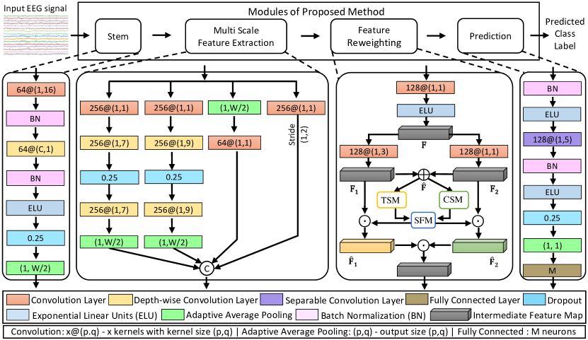
Figure 1: Detailed figure of the proposed network. It includes the complete framework of the proposed approach and all the modules of the proposed network in the first row. Each module expands in the second row of the figure through dotted lines. The second row of the figure shows the detailed layer stacking of each module. The third row represents the color coding of the layers, and the last row contains the description of operations used in the proposed network. Here, C: EEG channels, W: temporal data points, M: number of classes, $\copyright$: concatenation of the input feature maps, $\oplus$: addition of two feature maps, and $\odot$: Hadamard operation of two feature maps.

2.1 Proposed Network

The input EEG signals are defined as $E=\{(X_{i},Y_{i})|i=1,2,...,N\}$, where $X_{i}\in\texttt{R}^{C\times W}$ is a 2D array representing the $i^{th}$ EEG signal, $Y_{i}\in\{1,2,...M\}$ is the corresponding motor movement class, $N$ is the total number of EEG signals and $M$ represents the total classes of EEG signals. Here, $C$ and $W$ represent EEG electrodes and temporal data points of EEG signals, respectively. The proposed CNN-based network is shown in Fig. 1. The network consists of four modules: stem, multi-scale feature extraction, feature reweighting, and prediction. The details of these modules are given as follows :

2.1.1 Stem Module

The first module of the proposed method is named Stem and is similar to the first block of EEGNet [11]. At first, a convolution is applied to the input EEG signal to mix the temporal information. Afterward, a depth-wise convolution is applied to combine the EEG channels into a single channel and filter the spatial dependencies of the input signal. Exponential linear unit (ELU) [17] is opted as an activation function, followed by the dropout and adaptive average pooling [18] layer. This module is shown as "Stem" in Fig. 1.

2.1.2 Multi-Scale Feature Extraction Module

From the literature [5], it has been found that the effective convolution kernel size differs for different subjects. The reason is the physiological variations in the EEG signals that are subject-dependent and time-dependent [7]. Motivated by the finding of [5], the multi-scale kernel approach has been used via the Inception module [19]. This module extracts temporal information on multiple scales through multiple parallel branches that use different convolution kernel sizes. The temporal information on multiple scales helps to increase the EEG signal performance irrespective of the signal variations of each subject. This module is depicted as "Multi-Scale Feature Extraction" in Fig. 1.

2.1.3 Feature Reweighting Module

In the feature reweighting module (FRM), firstly, the output features from the multi-scale feature extraction module (MSF) are combined via a stack of convolution and ELU activation for mixing the information among various scales of MSF. The subsequent layers of FRM gives a relevance score by computing the score over temporal and channel dimensions of the feature maps. For computing the temporal and channel scores, two convolution operations are performed on the same feature maps $\mathbf{F}$ to obtain two different feature maps $\mathbf{F_{1}}$ and $\mathbf{F_{2}}$. A convolution operation with $1\times 3$ kernel size is applied to mix the temporal information of $\mathbf{F}$ feature maps to produce $\mathbf{F_{1}}$ feature maps. Similarly, a convolution operation with $1\times 1$ kernel size is applied to mix the channels of $\mathbf{F}$ feature maps to produce $\mathbf{F_{2}}$ feature maps. The output feature maps ($\mathbf{F_{1}}$ and $\mathbf{F_{2}}$) are added via element-wise summation to obtain $\hat{\textbf{F}}$ feature maps.

The temporal and channel feature scores are computed from $\hat{\textbf{F}}$ feature maps through the temporal feature score module (TSM) and channel feature score module (CSM). TSM and CSM compute the scores ($\mathbf{{S}}_{tsm}$ and $\mathbf{{S}}_{csm}$) by dropping the irrelevant information in feature maps across temporal and channel dimensions. These scores ($\mathbf{{S}}_{tsm}$ and $\mathbf{{S}}_{csm}$) are combined using the score fusion module (SFM). ). SFM gives feature reweighting scores $\mathbf{\hat{S}}_{tsm}$ and $\mathbf{\hat{S}}_{csm}$, that are used to filter the feature maps $\mathbf{F_{1}}$ and $\mathbf{F_{2}}$, respectively. Inspired by [20], the scores ($\mathbf{\hat{S}}_{tsm}$ and $\mathbf{\hat{S}}_{csm}$) are multiplied with the previous features maps ($\mathbf{F_{1}}$ and $\mathbf{F_{2}}$) to obtain less irrelevant and more relevant features maps ($\mathbf{{\hat{F}_{1}}}$ and $\mathbf{{\hat{F}_{2}}}$). The feature reweighting is performed using the following equations,

$$\mathbf{{\hat{F}_{1}}}=\mathbf{\hat{S}}_{tsm}\circ\mathbf{F_{1}}$$ (1)

$$\mathbf{{\hat{F}_{2}}}=\mathbf{\hat{S}}_{csm}\circ\mathbf{F_{2}}$$ (2)

where $\circ$ is a Hadamard product.

The systematic connection of these sub-modules (TSM, CSM and SFM) is shown under the module "Feature Reweighting" in Fig. 1. These sub-modules are further discussed in detail in Section 2.2.

2.1.4 Prediction Module

The features extracted from the feature reweighting module are passed to the prediction module to predict the category of the input MI-EEG signal. Inspired by [21], global average pooling layer has been included before the classifier. It makes the architecture context independent of the signal length. Finally, a fully connected layer is stacked for classification into M categories.

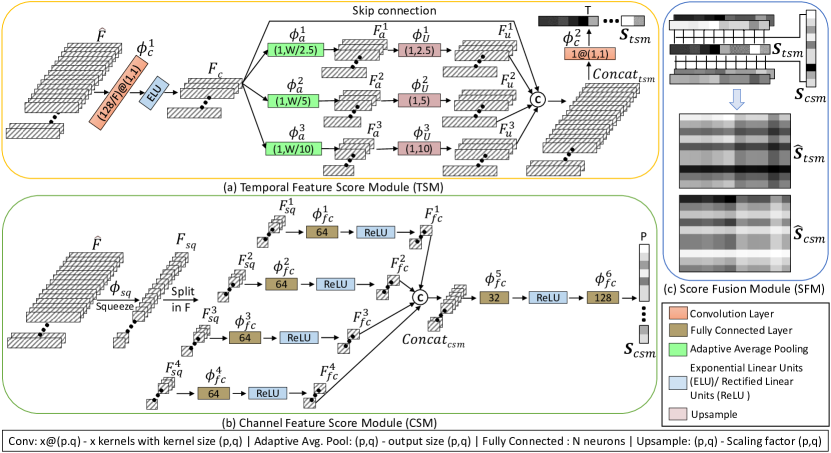
Figure 2: (a) Temporal Feature Score Module (TSM), (b) Channel Feature Score Module (CSM), (c) Score Fusion Module (SFM). Here, $\copyright$ symbol represents the concatenation of the input feature maps. The box below the (c) module shows the color coding of the layer operations used in these modules. The last horizontal box contains the description of the layer operations.

2.2 Feature Reweighting Submodules

The sub-modules of the feature reweighting module, named as temporal feature score module, channel feature score module, and score fusion module, are shown in Fig. 2. The details of these sub-modules are covered in the following subsections:

2.2.1 Temporal Feature Score Module:

The EEG data is a high-resolution temporal sequence of brain signals, and the EEG signal often gets mixed with other physiological and muscular information [6]. The relevant temporal information mixed with non-important information limits the MI-EEG classification performance. To handle it, the temporal feature score module intelligently learns the score of feature relevance, such that the relevant temporal features get a high score and irrelevant features get a low score.

In this module, at first, a convolution operation ($\phi_{c}^{1}$) is applied to the input feature maps $\hat{\textbf{F}}$ using the following equation,

$$\mathbf{F}_{c}=ELU(\phi_{c}^{1}(\hat{\mathbf{F}}))$$ (3)

where ELU is the activation function. The output feature maps ($\textbf{F}_{c}$) are then adaptive average pooled to different scales ($s_{i}$). The scales are given by the following equation,

$$s_{i}=\begin{matrix}\alpha.2^{i-1},&i=1,2,3\end{matrix}$$ (4)

where $\alpha$ is taken as $2.5$ and $s_{i}$ determines the scale of adaptive average pool. Adaptive average pooling operation extracts the features at different temporal lengths. The adaptive average pooling ($\phi_{a}^{i}$) is performed using the following equation,

$$\mathbf{F}_{a}^{i}=\begin{matrix}\phi_{a}^{i}(\mathbf{F}_{c},s_{i}),&i=1,2,3\end{matrix}$$ (5)

The features maps ($\textbf{F}_{a}^{i}$) are then upsampled to the original temporal length to re-scale the relevant features. The scale of upsampling is $s_{i}$, i.e., same as equation (4). Upsampling operation ($\phi_{u}^{i}$) depicted in following equation,

$$\mathbf{F}_{u}^{i}=\begin{matrix}\phi_{u}^{i}(\mathbf{F}_{a}^{i},s_{i})&i=1,2,3\end{matrix}$$ (6)

All feature maps ($\textbf{F}_{u}^{i}$) obtained from the $\phi_{u}^{i}$ upsampling operation are concatenated with $\textbf{F}_{c}$ using the following equation,

$$\mathbf{Concat}_{tsm}=[\mathbf{F}_{c}|\mathbf{F}_{u}^{1}|\mathbf{F}_{u}^{2}|\mathbf{F}_{u}^{3}]$$ (7)

where [$x|y$] represents the concatenation of two feature maps $x$ and $y$. Three scales ($s_{1}$, $s_{2}$ and $s_{3}$) from equation (5) and a skip connection of $\mathbf{F_{c}}$ shown in Fig. 2 (a) gives a total of four (4) scales. This scale factor is denoted by the time scale factor ($\beta$). In this work, value of $\beta$ is taken as 4. A convolution operation ($\phi_{c}^{2}$) is then performed on the concatenated feature maps to obtain a one-dimensional temporal feature score ($\mathbf{S}_{tsm}\in\texttt{R}^{T}$, $T$ is temporal length). The following equation derives the temporal feature score ($\textbf{S}_{tsm}$),

$$\mathbf{S}_{tsm}=\phi_{c}^{2}(\mathbf{Concat}_{tsm})$$ (8)

2.2.2 Channel Feature Score Module

The first step to compute the channel feature score is to squeeze the input feature maps $\mathbf{\hat{F}}$ obtained from the previous operation. This step is performed to explicitly select the relevant features that correspond to the respective feature map channel. The squeeze operation ($\phi_{sq}$) is defined as follows,

$$\mathbf{F}_{sq}=\phi_{sq}(\mathbf{\hat{F}})=\frac{1}{h\times w}\sum_{i=1}^{w}\sum_{j=1}^{h}\mathbf{\hat{F}}(i,j)$$ (9)

where $\mathbf{F}_{sq}$ is the squeezed feature maps. $h$ and $w$ are the height and width of $\mathbf{\hat{F}}$ feature maps, respectively. For efficient channel feature extraction, inspiration has been taken from [22]. The feature maps can be split into sets of multiple feature maps and then transformed separately for better and relevant feature extraction [22]. This splitting is done through the channel split factor ($\gamma$). In this work, the value of $\gamma$ is taken as $4$. The split operation gives $\gamma$ sets of feature maps ($\mathbf{F}_{sq}^{1}$, $\mathbf{F}_{sq}^{2}$, $\mathbf{F}_{sq}^{3}$, and $\mathbf{F}_{sq}^{4}$).

Thereafter, for each $\mathbf{F}_{sq}^{i}\in\texttt{R}^{s}$, a fully connected layer operation ($\phi_{fc}^{i}$) is performed to reduce the feature maps size to half i.e. $\mathbf{F}_{fc}^{i}\in\texttt{R}^{\frac{s}{2}}$ using the following equation,

$$\mathbf{F}_{fc}^{i}=\begin{matrix}ReLU(\phi_{fc}^{i}(\mathbf{F}_{sq}^{i}))&i=1,2,3,4\end{matrix}$$ (10)

where Rectified Linear Unit (ReLU) is used as the activation function of the fully connected layer. All of the output feature maps ($\mathbf{F}_{fc}^{1}$, $\mathbf{F}_{fc}^{2}$, $\mathbf{F}_{fc}^{3}$ and $\mathbf{F}_{fc}^{4}$) of the fully connected layer operation $\phi_{fc}^{i}$ are then concatenated with the help of following equation,

$$\mathbf{Concat}_{csm}=[\mathbf{F}_{fc}^{1}|\mathbf{F}_{fc}^{2}|\mathbf{F}_{fc}^{3}|\mathbf{F}_{fc}^{4}]$$ (11)

where [$x|y$] represents the concatenation of two feature maps $x$ and $y$. The channel feature score ($\mathbf{S}_{csm}\in\texttt{R}^{P}$, P is no. of channels) is then obtained using the following equation,

$$\mathbf{S}_{csm}=\phi_{{fc}}^{6}(ReLU(\phi_{fc}^{5}(\mathbf{Concat}_{csm})))$$ (12)

where $\phi_{{fc}^{5}}$ and $\phi_{{fc}^{6}}$ are fully connected layer operations that are used for the projection of the feature maps to the P dimension.

2.2.3 Score Fusion Module

The temporal feature score ($\mathbf{S}_{tsm}$) and channel feature score ($\mathbf{S}_{csm}$) are fused to compute the feature reweighting scores ($\mathbf{\hat{S}}_{tsm}$ and $\mathbf{\hat{S}}_{csm}$). The fusion of the scores is carried out through the following equations,

$$\mathbf{\hat{S}}_{tsm}^{(i,j)}=\frac{e^{\mathbf{S}_{tsm}^{(i,j)}}}{e^{\mathbf{S}_{tsm}^{(i,j)}}+e^{\mathbf{S}_{csm}^{(i,j)}}}$$ (13)

$$\mathbf{\hat{S}}_{csm}^{(i,j)}=\frac{e^{\mathbf{S}_{csm}^{(i,j)}}}{e^{\mathbf{S}_{tsm}^{(i,j)}}+e^{\mathbf{S}_{csm}^{(i,j)}}}$$ (14)

3 Experimental Results

3.1 Datasets

In this work, two publicly available motor imagery EEG datasets have been used to validate the performance and generalizability of the proposed method. The detailed description of the datasets are as follows:

3.1.1 Physionet EEGMMIDB dataset

The motor imagery dataset used in this work is from Physionet [23]. In this work, four motor imagery tasks, namely, right fist, left fist, both fists and both feet have been taken for analysis. The data is recorded on $64$ EEG electrodes with a sampling rate of $160$ Hz. It contains data from $109$ subjects. All $64$ EEG electrodes and the time segment of $0-4$ seconds after the onset of the visual cue are used in this work. Six subjects ($38$, $88$, $89$, $92$, $100$, and $104$) out of $109$, are dropped from the dataset due to different sampling rates and wrong labeling. The pre-processing of this dataset is same as [24]. In this work, ’PYD’ will be used for this dataset in the rest of the paper.

3.1.2 BCI Competition IV 2a dataset

BCI Competition IV 2a dataset [25] is a collection of motor imagery EEG data of nine healthy participants. The dataset contains EEG signals corresponding to four MI tasks, namely, left-hand, right-hand, both feet, and tongue. All of these tasks are used in this work. The EEG signals were recorded using $22$ EEG electrodes with a sampling rate of $250$ Hz. All $22$ EEG electrodes and the time segment of $0-4$ seconds after the onset of the visual cue are used in this work. The pre-processing of this dataset is the same as [12, 26]. In the rest of the paper, the name ’BCI’ will be used for this dataset.

3.2 Experimental Setup

The proposed method has been trained using a Xeon processor with $96$GB RAM and Nvidia Quadro P5000 with $16$GB of GPU RAM. The proposed model has been initialized with Xavier method [27] and trained for $200$ epochs with Adam optimizer [28] with an initial learning rate of $0.001$ and weight decay of $10^{-4}$. The model has been trained with a batch size of $64$. The proposed model learns the classification of data by minimizing the prominently used cross-entropy loss [29]. A widely used five-fold cross-validation technique is employed for both datasets to obtain generalized results and fair comparison among methods. Also, the same experimental settings are used for both the analyzed datasets.

3.3 Metrics

In this work, the metrics used for the evaluation of MI-EEG classification are accuracy, f-measure, and Kappa measure. In addition, AUC-ROC curve plots are used to measure the degree of separability of the model among various classes. Furthermore, the paired t-test method is employed to measure the statistical significance of the proposed method over the compared methods.

Table 1: Detailed results of the proposed method on the BCI dataset.

Subject	Accuracy	F-measure	Kappa
A01	85.54 $\pm$ 3.02	0.85 $\pm$ 0.03	0.81 $\pm$ 0.04
A02	60.89 $\pm$ 5.38	0.61 $\pm$ 0.06	0.48 $\pm$ 0.07
A03	93.75 $\pm$ 1.95	0.94 $\pm$ 0.02	0.92 $\pm$ 0.03
A04	78.16 $\pm$ 4.12	0.78 $\pm$ 0.04	0.71 $\pm$ 0.05
A05	72.67 $\pm$ 3.81	0.72 $\pm$ 0.04	0.63 $\pm$ 0.05
A06	69.39 $\pm$ 5.47	0.69 $\pm$ 0.05	0.59 $\pm$ 0.07
A07	93.80 $\pm$ 3.25	0.94 $\pm$ 0.03	0.92 $\pm$ 0.04
A08	88.22 $\pm$ 3.94	0.88 $\pm$ 0.04	0.84 $\pm$ 0.05
A09	83.64 $\pm$ 3.42	0.83 $\pm$ 0.04	0.78 $\pm$ 0.05

Table 2: Comparison of the proposed method with various state-of-the-art (SOTA) methods for motor imagery task. Best values are bold-faced. [D: Dataset, M: Metric, A: Accuracy, F: F-measure, K: Kappa, p: p-value]

D	M	Methods
		FBCSP [30]	TS-Net [16]	EEGNet [11]	Fusion [24]	MI-Net [26]	Deep [12]	Shallow [12]	Proposed
PYD	A	30.63 $\pm$ 0.53	57.31 $\pm$ 1.06	37.53 $\pm$ 1.63	73.73 $\pm$ 1.32	85.71 $\pm$ 3.52	57.66 $\pm$ 2.23	70.16 $\pm$ 0.28	95.05 $\pm$ 2.11
	F	0.30 $\pm$ 0.01	0.57 $\pm$ 0.01	0.36 $\pm$ 0.03	0.74 $\pm$ 0.01	0.86 $\pm$ 0.04	0.57 $\pm$ 0.03	0.7 $\pm$ 0.00	0.95 $\pm$ 0.02
	K	0.03 $\pm$ 0.01	0.49 $\pm$ 0.48	0.17 $\pm$ 0.02	0.65 $\pm$ 0.02	0.81 $\pm$ 0.05	0.44 $\pm$ 0.03	0.60 $\pm$ 0.00	0.93 $\pm$ 0.03
	p	$<0.05$	$<0.05$	$<0.05$	$<0.05$	$<0.05$	$<0.05$	$<0.05$	$-$
BCI	A	69.56 $\pm$ 13.58	53.43 $\pm$ 12.49	62.39 $\pm$ 9.32	66.39 $\pm$ 8.91	75.85 $\pm$ 11.93	65.66 $\pm$ 15.90	76.85 $\pm$ 13.66	80.67 $\pm$ 11.30
	F	0.69 $\pm$ 0.14	0.50 $\pm$ 0.14	0.62 $\pm$ 0.09	0.62 $\pm$ 0.09	0.76 $\pm$ 0.12	0.64 $\pm$ 0.17	0.77 $\pm$ 0.14	0.80 $\pm$ 0.11
	K	0.59 $\pm$ 0.18	0.38 $\pm$ 0.16	0.5 $\pm$ 0.12	0.55 $\pm$ 0.12	0.68 $\pm$ 0.16	0.54 $\pm$ 0.21	0.69 $\pm$ 0.18	0.74 $\pm$ 0.15
	p	$<0.05$	$<0.05$	$<0.05$	$<0.05$	$<0.05$	$<0.05$	$<0.05$	$-$

3.4 Classification Performance

In this section, the classification performance of the proposed method for BCI and PYD datasets has been discussed in detail. Along with the performance of these datasets, a rigorous comparison has also been reported. The methods considered for the comparison are filter bank common spatial patterns (FBCSP) [30], EEGNet [11], EEGNet Fusion [24] (depicted as Fusion), MI-EEGNet [26] (depicted as MI-Net), TS-SEFFNet [16] (depicted as TS-Net), DeepConvNet (depicted as Deep) [12] and ShallowConvNet (depicted as Shallow) [12]. The detailed results of the proposed method for BCI and PYD datasets are summarized in Table 1 and 2.

The average accuracy of proposed method for the BCI dataset is $80.67\%$. Table 1 shows that five subjects (A01, A03, A07, A08 and A09) have an accuracy of more than $80\%$. A similar pattern can be observed for F-measure and Kappa metrics. It shows the good prediction performance of the proposed method. Fig. 3 and Fig. 4 show the confusion matrices and roc curve plots of both datasets, respectively. These figures show a balanced class-wise decoding performance of the proposed method for both datasets. Therefore, the good performance of the proposed method for both datasets validates the need for feature reweighting in MI-EEG classification.

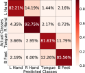
(a) BCI A01

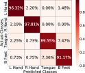
(b) BCI A03

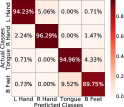
(c) BCI A07

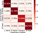
(d) BCI A08

(e) PYD

Figure 3: Confusion matrices of the proposed method for four subjects (A01, A03, A07 and A08) of BCI dataset and PYD dataset.

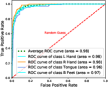
(a) BCI A01

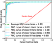
(b) BCI A03

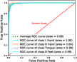
(c) BCI A07

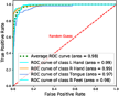
(d) BCI A08

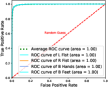
(e) PYD

Figure 4: ROC curves of the proposed method for four subjects (A01, A03, A07, and A08) of BCI dataset and PYD dataset.

Table 2 shows that for the PYD dataset, the proposed method outperforms all the compared methods by a massive margin of $9.34\%$ in the accuracy metric. The p-value also suggests that the proposed method is more statistically significant than the compared methods. For the BCI dataset, the proposed method shows better classification accuracy than the compared methods with a margin of $3.82\%$ in accuracy. The p-value of the proposed method versus all compared methods is less than $0.05$. Therefore, the performance of the proposed method has fair statistical significance over the compared methods.

Additionally, the famous traditional machine learning method FBCSP [30] is also considered for comparison. The proposed method performs better than the FBCSP in both BCI and PYD datasets. However, Table 2 shows that for the BCI dataset, FBCSP has performed superior to three of the other CNN-based methods (EEGNet, EEGNet Fusion and Deep ConvNet). It shows the significance of extracting features using filter bank and common spatial patterns over conventional CNN-based approaches such as EEGNet, EEGNet Fusion, and Deep ConvNet. However, the usage of feature reweighting is found to be superior as the feature reweighting mechanism helps to filter out irrelevant information efficiently. As a result, the proposed method outperforms FBCSP. Thus, proposed method performed significantly better than all of the compared methods.

4 Discussion

Table 3: Ablation study to compute the impact of FRM and MSF. Best values are bold-faced.

Variant	Accuracy
	PYD	BCI
w/o FRM	89.20 $\pm$ 1.37	74.01 $\pm$ 12.40
w/o MSF	91.93 $\pm$ 1.24	77.84 $\pm$ 12.31
FRM + MSF (proposed)	95.05 $\pm$ 2.11	80.67 $\pm$ 11.30

4.1 Ablation study

In this section, a detailed ablation study is conducted to understand the effectiveness of each component of the proposed method. This ablation comprises an in-depth understanding of the impact of FRM, MSF, TSM and CSM. Additionally, the impact of the time scale factor ($\beta$) of TSM and the channel split factor ($\gamma$) of CSM on the classification performance is discussed.

4.1.1 Impact of Feature Reweighting Module (FRM) and Multi-Scale Feature Extraction Module (MSF) on EEG classification

In the proposed method, two important modules used for feature extraction are the multi-scale feature extraction module (MSF) and the feature reweighting module (FRM). In this ablation, the proposed method is compared with its two variants obtained by removing either MSF or FRM from the proposed model. The model without the MSF module is symbolized by w/o MSF, and the model without FRM by w/o FRM. FRM + MSF symbolizes the proposed method. The performance of these models is summarized in Table 3. It shows that the impact of FRM is more than MSF in terms of MI-EEG classification accuracy in both datasets. It implies that the model without multi-scale feature extraction (w/o MSF) can extract more relevant features of the EEG signal and obtain better results. If the MSF is combined with the FRM (i.e., the proposed method), it is better than the two variants for both datasets. It also shows the usefulness of the feature reweighting mechanism in getting better MI-EEG classification.

Table 4: Ablation study to compute the impact of sub-modules of FRM (TSM and CSM) on each subject of BCI dataset.

TSM	CSM	A01	A02	A03	A04	A05	A06	A07	A08	A09
✗	✗	78.93 $\pm$ 6.25	55.39 $\pm$ 6.13	89.50 $\pm$ 2.66	66.53 $\pm$ 2.83	67.06 $\pm$ 4.70	60.17 $\pm$ 3.51	89.25 $\pm$ 3.29	83.36 $\pm$ 2.83	75.86 $\pm$ 3.00
✗	✓	85.40 $\pm$ 2.64	60.05 $\pm$ 2.02	92.27 $\pm$ 2.12	78.98 $\pm$ 5.23	71.36 $\pm$ 3.17	66.20 $\pm$ 5.65	93.62 $\pm$ 3.21	87.29 $\pm$ 3.89	83.83 $\pm$ 2.87
✓	✗	84.65 $\pm$ 3.19	56.61 $\pm$ 3.89	93.37 $\pm$ 2.74	75.71 $\pm$ 4.91	73.05 $\pm$ 2.76	68.24 $\pm$ 4.44	94.54 $\pm$ 2.70	88.79 $\pm$ 4.72	84.43 $\pm$ 3.92
✓	✓	85.54 $\pm$ 3.02	60.89 $\pm$ 5.38	93.75 $\pm$ 1.95	78.16 $\pm$ 4.12	72.67 $\pm$ 3.81	69.39 $\pm$ 5.47	93.80 $\pm$ 3.25	88.22 $\pm$ 3.94	83.64 $\pm$ 3.42

Table 5: Ablation study to compute the impact of sub-modules of FRM. Best values are bold-faced.

TSM	CSM	Accuracy
		PYD	BCI
✗	✗	89.20 $\pm$ 1.37	74.01 $\pm$ 12.40
✗	✓	94.19 $\pm$ 1.87	79.89 $\pm$ 11.71
✓	✗	94.62 $\pm$ 2.60	79.93 $\pm$ 12.55
✓	✓	95.05 $\pm$ 2.11	80.67 $\pm$ 11.30

4.1.2 Impact of Temporal Feature Score Module (TSM) and Channel Feature Score Module (CSM) on EEG classification

The feature reweighting mechanism is based on the score computed by TSM and CSM. This ablation is conducted to explore the different combinations of the TSM and CSM and to observe their impact on MI-EEG classification. It results in four variants of the proposed method. The subject-wise and average classification performance of these four variants is summarized in Table 4 and Table 5. Table 4 and Table 5 show that the variant that does not have TSM and CSM has the lowest classification performance for both datasets. It is also observed from Table 5 that the impact of individual TSM and CSM seems similar. However, Table 4 shows that TSM performs better than CSM for six subjects (A03, A05, A06, A07, A08, and A09) of the BCI dataset. Therefore, the TSM is found to be performing better than the CSM. Finally, adding TSM and CSM to the feature reweighting mechanism (i.e., the proposed method) helps to elevate the classification performance in both datasets.

Table 6: Ablation study on factors ($\beta$ and $\gamma$) of FRM. Best values are bold-faced. [D: Dataset, S: Subject, Avg.: Average]

D	S	Accuracy
		($\beta$, $\gamma$)=(3,3)	($\beta$, $\gamma$)=(4,4)	($\beta$, $\gamma$)=(5,5)
BCI	A01	86.08 $\pm$ 2.71	85.54 $\pm$ 3.02	84.82 $\pm$ 2.21
	A02	58.22 $\pm$ 2.35	60.89 $\pm$ 5.38	58.59 $\pm$ 4.20
	A03	93.37 $\pm$ 0.32	93.75 $\pm$ 1.95	92.64 $\pm$ 1.43
	A04	78.57 $\pm$ 4.73	78.16 $\pm$ 4.12	80.82 $\pm$ 3.34
	A05	71.57 $\pm$ 3.29	72.67 $\pm$ 3.81	72.51 $\pm$ 4.43
	A06	65.91 $\pm$ 2.73	69.39 $\pm$ 5.47	67.04 $\pm$ 3.92
	A07	92.52 $\pm$ 1.77	93.80 $\pm$ 3.25	94.15 $\pm$ 3.03
	A08	89.16 $\pm$ 4.70	88.22 $\pm$ 3.94	88.04 $\pm$ 5.39
	A09	85.03 $\pm$ 2.22	83.64 $\pm$ 3.42	85.63 $\pm$ 2.89
	Avg.	80.05 $\pm$ 12.39	80.67 $\pm$ 11.30	80.47 $\pm$ 12.05
PYD	Avg.	93.52 $\pm$ 0.68	95.05 $\pm$ 2.11	94.76 $\pm$ 2.56

4.1.3 Impact of time scale factor ($\beta$) and channel split factor ($\gamma$) on Feature Reweighting Module

The proposed FRM relies on efficient temporal and channel score computation. The temporal and channel score computation module is designed over the time scale factor ($\beta$) and channel split factor ($\gamma$), respectively. Hence, the impact of these hyper-parameters in the network design is investigated in this ablation. The ablation results are shown in Table 6. For ease of understanding, the same increment rate for both factors is followed in this study. From this ablation study, it can be observed that the optimal value for factors ($\beta$, $\gamma$) is ($4$, $4$) for both datasets (i.e., the value chosen for the proposed method). On further subject-wise analysis of the impact of factors, again, the factor ($4$, $4$) is preferred over the other factor values. Thus, it is concluded that the optimal value of the factors ($\beta$, $\gamma$) is ($4$,$4$) for this work.

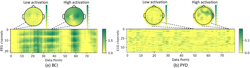
Figure 5: Grad-CAM activation maps with corresponding topographical plots of (a) BCI dataset and (b) PYD dataset. The brighter regions imply high attention, and the darker regions imply low attention to the input signal data points.

4.2 Grad-CAM visualization

Grad-CAM is a popular method used to visualize the importance of the features extracted by a machine learning method [31]. The grad-CAM activation maps obtained from the proposed method are shown in Fig. 5. Grad-CAM attention maps of both datasets show a repeated pattern of bright and dark regions. The protocol of the motor imagery task is the reason behind the observed pattern. In both datasets, the subjects were instructed to repetitively perform the particular motor imagery task until the trial ended. Therefore, the bright regions in the grad-CAM activation maps correspond to the time instances of brain activity, and the dark region corresponds to the time instances of brain inactivity. Additionally, topographical plots of low and high activation instances are shown above the grad-CAM activation maps in Fig. 5. The high activation topographical plots of both datasets show increased activation in sensorimotor areas, whereas low activation plots show activity in other brain regions. It indicates that the proposed method gives high importance to the relevant features and low importance to irrelevant features of the MI-EEG signals.

5 Conclusion

This work proposes a novel feature reweighting approach that helps in suppressing the noisy and irrelevant features, and emphasizing the relevant features of the MI-EEG signals. The proposed network performs better than many state-of-the-art approaches on two publicly available datasets for motor imagery classification. The proposed method outperformed the compared methods in classification accuracy by a margin of $9.34\%$ and $3.82\%$ in PYD and BCI datasets, respectively. Also, the variants of the proposed network that contain the individual temporal feature score module (TSM) and channel feature score module (CSM) outperformed the compared methods in classification accuracy by $8.91\%$ and $8.48\%$ in the PYD dataset and $3.08\%$ and $2.04\%$ in the BCI dataset. It indicates that the reduction of noise and irrelevant feature across both temporal and channel dimension of feature maps has significant impact on the classification performance. The performance of the proposed method on the motor movement task is competitive. It shows the robustness and generalizability of the proposed method. In the future, the proposed method can be used in other EEG-based BCI paradigms for classification.

References

- [1] Floriana Pichiorri, Giovanni Morone, Manuela Petti, Jlenia Toppi, Iolanda Pisotta, Marco Molinari, Stefano Paolucci, Maurizio Inghilleri, Laura Astolfi, Febo Cincotti, et al. Brain–computer interface boosts motor imagery practice during stroke recovery. Annals of Neurology, 77(5):851–865, 2015.
- [2] Nataliya Kosmyna, Franck Tarpin-Bernard, Nicolas Bonnefond, and Bertrand Rivet. Feasibility of bci control in a realistic smart home environment. Frontiers in Human Neuroscience, 10:416, 2016.
- [3] Yiliang Liu, Wenbin Su, Zhijun Li, Guangming Shi, Xiaoli Chu, Yu Kang, and Weiwei Shang. Motor-imagery-based teleoperation of a dual-arm robot performing manipulation tasks. IEEE Transactions on Cognitive and Developmental Systems, 11(3):414–424, 2018.
- [4] Ranganatha Sitaram, Haihong Zhang, Cuntai Guan, Manoj Thulasidas, Yoko Hoshi, Akihiro Ishikawa, Koji Shimizu, and Niels Birbaumer. Temporal classification of multichannel near-infrared spectroscopy signals of motor imagery for developing a brain–computer interface. NeuroImage, 34(4):1416–1427, 2007.
- [5] Guanghai Dai, Jun Zhou, Jiahui Huang, and Ning Wang. HS-CNN: a CNN with hybrid convolution scale for EEG motor imagery classification. Journal of Neural Engineering, 17(1):1–11, 2020.
- [6] Xiao Jiang, Gui-Bin Bian, and Zean Tian. Removal of artifacts from EEG signals: a review. Sensors, 19(5):1–18, 2019.
- [7] Femke Nijboer, Niels Birbaumer, and Andrea Kübler. The influence of psychological state and motivation on brain–computer interface performance in patients with amyotrophic lateral sclerosis–a longitudinal study. Frontiers in Neuropharmacology, 4:55, 2010.
- [8] Simanto Saha, Khawza Iftekhar Uddin Ahmed, Raqibul Mostafa, Leontios Hadjileontiadis, and Ahsan Khandoker. Evidence of variabilities in eeg dynamics during motor imagery-based multiclass brain–computer interface. IEEE Transactions on Neural Systems and Rehabilitation Engineering, 26(2):371–382, 2017.
- [9] Kai Keng Ang, Zheng Yang Chin, Chuanchu Wang, Cuntai Guan, and Haihong Zhang. Filter bank common spatial pattern algorithm on bci competition iv datasets 2a and 2b. Frontiers in Neuroscience, 6:39, 2012.
- [10] Lie Yang, Yonghao Song, Ke Ma, and Longhan Xie. Motor imagery eeg decoding method based on a discriminative feature learning strategy. IEEE Transactions on Neural Systems and Rehabilitation Engineering, 29:368–379, 2021.
- [11] Vernon J Lawhern, Amelia J Solon, Nicholas R Waytowich, Stephen M Gordon, Chou P Hung, and Brent J Lance. EEGNet: a compact convolutional neural network for EEG-based brain–computer interfaces. Journal of Neural Engineering, 15(5):1–17, 2018.
- [12] Robin Tibor Schirrmeister, Jost Tobias Springenberg, Lukas Dominique Josef Fiederer, Martin Glasstetter, Katharina Eggensperger, Michael Tangermann, Frank Hutter, Wolfram Burgard, and Tonio Ball. Deep learning with convolutional neural networks for eeg decoding and visualization. Human Brain Mapping, 38(11):5391–5420, 2017.
- [13] Yann LeCun, Yoshua Bengio, and Geoffrey Hinton. Deep learning. Nature, 521(7553):436–444, 2015.
- [14] Bingyi Kang, Zhuang Liu, Xin Wang, Fisher Yu, Jiashi Feng, and Trevor Darrell. Few-shot object detection via feature reweighting. In Proceedings of the IEEE/CVF International Conference on Computer Vision, pages 8420–8429, 2019.
- [15] Xin Zhao, Zhe Liu, Ruolan Hu, and Kaiqi Huang. 3d object detection using scale invariant and feature reweighting networks. In Proceedings of the AAAI Conference on Artificial Intelligence, volume 33, pages 9267–9274, 2019.
- [16] Yang Li, Lianghui Guo, Yu Liu, Jingyu Liu, and Fangang Meng. A temporal-spectral-based squeeze-and-excitation feature fusion network for motor imagery eeg decoding. IEEE Transactions on Neural Systems and Rehabilitation Engineering, 29:1534–1545, 2021.
- [17] Djork-Arné Clevert, Thomas Unterthiner, and Sepp Hochreiter. Fast and accurate deep network learning by exponential linear units (elus). arXiv preprint arXiv:1511.07289, 2015.
- [18] Elahe Rahimian, Soheil Zabihi, Seyed Farokh Atashzar, Amir Asif, and Arash Mohammadi. Xceptiontime: independent time-window xceptiontime architecture for hand gesture classification. In ICASSP 2020-2020 IEEE International Conference on Acoustics, Speech and Signal Processing (ICASSP), pages 1304–1308. IEEE, 2020.
- [19] Christian Szegedy, Wei Liu, Yangqing Jia, Pierre Sermanet, Scott Reed, Dragomir Anguelov, Dumitru Erhan, Vincent Vanhoucke, and Andrew Rabinovich. Going deeper with convolutions. In Proceedings of the IEEE Conference on Computer Vision and Pattern Recognition, pages 1–9, 2015.
- [20] Xiang Li, Wenhai Wang, Xiaolin Hu, and Jian Yang. Selective kernel networks. In Proceedings of the IEEE/CVF Conference on Computer Vision and Pattern Recognition, pages 510–519, 2019.
- [21] Forrest N Iandola, Song Han, Matthew W Moskewicz, Khalid Ashraf, William J Dally, and Kurt Keutzer. SqueezeNet: AlexNet-level accuracy with 50x fewer parameters and 0.5 mb model size. arXiv preprint arXiv:1602.07360, 2016.
- [22] Xiangyu Zhang, Xinyu Zhou, Mengxiao Lin, and Jian Sun. Shufflenet: An extremely efficient convolutional neural network for mobile devices. In Proceedings of the IEEE Conference on Computer Vision and Pattern Recognition, pages 6848–6856, 2018.
- [23] Ary L Goldberger, Luis AN Amaral, Leon Glass, Jeffrey M Hausdorff, Plamen Ch Ivanov, Roger G Mark, Joseph E Mietus, George B Moody, Chung-Kang Peng, and H Eugene Stanley. PhysioBank, PhysioToolkit, and PhysioNet: components of a new research resource for complex physiologic signals. Circulation, 101(23):e215–e220, 2000.
- [24] Karel Roots, Yar Muhammad, and Naveed Muhammad. Fusion convolutional neural network for cross-subject EEG motor imagery classification. Computers, 9(3):1–9, 2020.
- [25] Michael Tangermann, Klaus-Robert Müller, Ad Aertsen, Niels Birbaumer, Christoph Braun, Clemens Brunner, Robert Leeb, Carsten Mehring, Kai J Miller, Gernot Mueller-Putz, et al. Review of the BCI competition IV. Frontiers in Neuroscience, 6:1–31, 2012.
- [26] Mouad Riyad, Mohammed Khalil, and Abdellah Adib. MI-EEGNET: A novel convolutional neural network for motor imagery classification. Journal of Neuroscience Methods, 353:1–11, 2021.
- [27] Xavier Glorot and Yoshua Bengio. Understanding the difficulty of training deep feedforward neural networks. In Proceedings of the Thirteenth International Conference on Artificial Intelligence and Statistics, pages 249–256, 2010.
- [28] Diederik P Kingma and Jimmy Ba. Adam: A method for stochastic optimization. arXiv preprint arXiv:1412.6980, 2014.
- [29] Taveena Lotey, Prateek Keserwani, Gaurav Wasnik, and Partha Pratim Roy. Cross-session motor imagery eeg classification using self-supervised contrastive learning. In Proceedings of the IEEE International Conference on Pattern Recognition, pages 1–7, 2022.
- [30] Kai Keng Ang, Zheng Yang Chin, Haihong Zhang, and Cuntai Guan. Filter bank common spatial pattern (fbcsp) in brain-computer interface. In 2008 IEEE international Joint Conference on Neural Networks (IEEE world Congress on Computational Intelligence), pages 2390–2397. IEEE, 2008.
- [31] Ramprasaath R Selvaraju, Michael Cogswell, Abhishek Das, Ramakrishna Vedantam, Devi Parikh, and Dhruv Batra. Grad-cam: Visual explanations from deep networks via gradient-based localization. In Proceedings of the IEEE International Conference on Computer Vision, pages 618–626, 2017.