The identification of garbage dumps in the rural areas of Cyprus through the application of deep learning to satellite imagery

Abstract

Garbage disposal is a challenging problem throughout the developed world. In Cyprus, as elsewhere, illegal “fly-tipping” is a significant issue, especially in rural areas where few legal garbage disposal options exist. However, there is a lack of studies that attempt to measure the scale of this problem, and few resources available to address it. A method of automating the process of identifying garbage dumps would help counter this and provide information to the relevant authorities.

The aim of this study was to investigate the degree to which artificial intelligence techniques, together with satellite imagery, can be used to identify illegal garbage dumps in the rural areas of Cyprus. This involved collecting a novel dataset of images that could be categorised as either containing, or not containing, garbage. The collection of such datasets in sufficient raw quantities is time consuming and costly. Therefore a relatively modest baseline set of images was collected, then data augmentation techniques used to increase the size of this dataset to a point where useful machine learning could occur.

From this set of images an artificial neural network was trained to recognise the presence or absence of garbage in new images. A type of neural network especially suited to this task known as “convolutional neural networks” was used. The efficacy of the resulting model was evaluated using an independently collected dataset of test images.

The result was a deep learning model that could correctly identify images containing garbage in approximately 90% of cases. It is envisaged that this model could form the basis of a future system that could systematically analyse the entire landscape of Cyprus to build a comprehensive “garbage” map of the island.

Keywords: garbage disposal, fly-tipping, artificial intelligence, satellite imagery, image augmentation, convolutional neural networks, deep learning, Cyprus.

1 Introduction

1.1 Background and Motivations

Illegal waste dumping is a social and environmental issue throughout the developed and developing world [1]. The consequences include environmental pollution, health hazards, and negative impacts on local ecosystems and aesthetics. The island of Cyprus has particular issues with waste disposal in rural areas[2], where little formal recycling exists. As a result, citizens tend to make impromptu garbage dumps. Assessing the scale of this issue is difficult [3]. However, if there was a way of identifying how many such garbage dumps have accumulated, together with their location, then this could be used to inform and exert pressure on local, regional and national government bodies to address the issue proactively [4].

Performing this sort of task by hand would be laborious and error prone. If, for example, the land was divided up into $100m^{2}$ patches, then even for a relatively modest sized country such as Cyprus covering around $9250km^{2}$ this would require at least 925,000 such image patches to be analysed. If a human could retrieve an image, visually analyse it, and store the classification result as an atomic operation in around one minute, then to classify all image patches would require more than 15,400 person hours or 640 days.

Some previous work has employed AI techniques to automatically detect the presence of garbage dumps, such as [5] and [6]. These projects have focused on large land-fills occupying an area of several square kilometers. Few such projects exist focusing on small scale sites covering just tens or hundreds of square metres. However, it is such small areas that Cyprus garbage dumps tend to occupy. With the existence of public access high resolution remote sensing imagery, such as satellite [7] [8], it is possible to focus on techniques to recognise these smaller scale features. This study utilised a type of Artificial Neural Network (ANN) shown to be effective in the classification of satellite imagery [9] and applied it to these small scale features.

1.2 Aims and Objectives

The aim of this study was to develop and evaluate an AI based approach for identifying garbage heaps in Cyprus. This involved the collection and labeling of satellite imagery. However, collection of such image sets is a laborious task and it is unfeasible to collect such “raw” data in sufficient quantities to perform useful machine learning [10]. To counter this, data augmentation techniques such as sharpening, cropping, rotating, and flipping were used to significantly increase the dataset sizes, whilst retaining the important features.

The questions the study sought answers to were:

• What are the most effective machine learning algorithms and techniques for developing a model that can accurately identify and classify small scale garbage dumps in the rural areas of Cyprus from satellite imagery?

• To what extent can data augmentation techniques improve a machine learning model for such small scale satellite image classification?

1.3 Approach

To provide answers to the questions above the following steps were completed. Data was collected in the form of satellite images of known garbage locations in Cyprus, forming a baseline dataset. This dataset was expanded through various data augmentation techniques [11]: sharpening, rotating, cropping, and flipping. A suitable machine learning model was selected for the study by training and evaluating various candidates against the baseline. The chosen model was then trained on the augmented datasets. Finally, the accuracy of the model was evaluated by applying various validation methods and statistics in order to arrive at conclusions with regards the efficacy of the model.

The study focused on a type of deep learning model referred to as convolutional neural networks (CNNs). These work by applying various filters to the images which learn to pick out low level then progressively higher level features from the images [12], culminating in, for this study, the identification of garbage. Dimensionality of the input data is reduced to a manageable level by use of such techniques as pooling [13]. CNNs have proven effective at image recognition, and have been applied successfully to the area of remote sensing [14].

1.4 Results and Contributions

The results and outputs of the study are manyfold:

• A novel baseline set of satellite image patches labelled as containing/not containing garbage, which might find use outside of this study.

• Several augmented datasets of similarly labelled images which may also find wider use within the machine learning community.

• A set of CNN models which provide an accurate basis for garbage heap identification with the potential to inform waste management policies in Cyprus.

1.5 Outline

Section 2 develops a theoretical framework to the study, mostly through a review of pertinent literature. Section 3 establishes the research methodology used to answer the research questions. This is followed by a discussion of the results in section 4 and finally a conclusion and recommendations for future work in section 5.

2 Theoretical Background

2.1 Motivations

Webb et al., 2006 [3] provide a comprehensive study into the incidence of fly-tipping. They describe in detail the who, how, where, and why of such practices and their environmental and social impact. One issue highlighted is the difficulty authorities have in mapping the location of fly-tipping sites - a main driver behind this research and one of the main objectives it seeks to address by producing models which can recognize garbage dumps from satellite images.

2.2 Deep Learning

The original deep learning research into image recognition was undertaken thirty years ago when LeCun used the Multilayer Perceptron with back-propagation to recognize handwritten digits [15]. Back-propagation is an iterative algorithm used to adjust the weights of the connections between nodes to minimize the difference between the predicted output and the actual output. It forms the basis by which Artificial Neural Networks (ANNs) are trained on input data. Since then deep learning has become the dominant method for all image recognition tasks, including those involving remote sensing sources such as satellite imagery. One of the main reasons for this is that an ANN can model complex non-linear relationships, as described by LeCun in the later 2015 paper [16].

Standard ANNs can be effective for classifying small image patches, but for complex large satellite images this is an impractical method. Each pixel of an image is a separate input to the network. Once multiple layers are added to the network then the number of parameters in the training process grows exponentially such that the training time and memory requirements become prohibitively high [17]. To address this a type of ANN called the Convolutional Neural Network (CNN) has become very popular.

2.3 Convolutional Neural Networks

The first CNN was proposed by Fukushima in the foundational 1980 paper [18] in which the neocognitron is described as an “improved neural network”. This is essentially a hierarchy of networks composed of layers of nodes with “variable connections between adjoining layers”. LeCun took this idea further in 1998 [19] in which back-propagation and gradient descent were added and he showed how these strategies could solve pattern recognition involving high dimensional images better than existing hand-designed algorithms. This lay the groundwork for future CNN algorithms and variations such as LeNet, AlexNet, Google LeNet, and ResNet. [20]. Much of the earlier work focused on recognition of small scale images, particularly that of handwritten characters [21]. Subsequently, this was adapted for larger scale satellite imagery.

2.4 Machine Learning and Satellite Imagery

Satellite imagery poses unique challenges for machine learning. Forkuor et al. (2018) extensively discuss these challenges in the context of land-use and land-cover mapping in Burkina Faso. Satellite images are larger and multi-spectral, with Sentinel-2 satellites offering 13 spectral bands, including near-infrared channels. This additional spectral information enables analysis of thermal characteristics, which can be relevant for certain types of garbage dumps containing biological matter. However, utilizing more channels in training a model increases the number of parameters and learning time. Consequently, this study opted to use three-channel RGB images.

Vaishnnave et al. (2019) provide a survey of different methods for classifying satellite datasets, including popular CNN algorithms like AlexNet, ResNet-50, GoogleNet, and CaffeNet. CNN methods exhibited the highest accuracy, ranging from 93% to 99%. It is important to note that these accuracy figures are drawn from various studies with different datasets and objectives, making direct comparisons challenging. Nonetheless, they lend support to the approach adopted in the current study.

A particularly relevant study by Rajkumar et al. (2022) applies various ML algorithms to landfills using satellite missions such as WorldView and GeoEye. The dataset comprised 245 images, each with dimensions of 512x512 pixels. Although the covered area is not specified, the landfills were significantly larger than those addressed in the current study. The results demonstrated accuracy ranging from 76% to 83%.

2.5 Residual Networks

Residual Networks (ResNets) are a successful subset of CNNs, particularly in remote sensing. He et al. introduced ResNets in 2016 to address the vanishing gradient problem, which hinders learning in deep networks. The influential paper proposes an architecture with shortcut connections between layers, allowing nodes to be treated as blocks during the learning process. This approach facilitates the smooth flow of gradients through deep networks. The paper demonstrates the capability of training networks with over 1000 layers using this method.

2.6 Pretrained Zoo Models

Pretrained models are specific implementations of ML algorithms that have been trained on large amounts of data. They can be used to “shortcut” the training time of similar problems and result in better models. The paper by Yosinski et al. 2014 [22] details early work that showed how even when the training data is significantly different from that of the target problem, that models designed around them perform better than not pretrained. It is not fully established why this is, but it might have something to do with the general structures that make up typical objects in 2D images being learned, such as edges, irrespective of what the target image is.

2.7 Data Collection

There are several potential sources of high resolution satellite data. The US geological survey provides Earth Explorer - a user interface into the Landsat satellite system [23]. Sentinel data is available from the ESA open access hub [24]. Forkuor (2018) [25] describes a study of these two sources for land use and land cover, and applied three ML algorithms to compare their relative performance. Of the two, the Sentinel data proved slightly more accurate than the Landsat, although the algorithms were not ANN based, which tempers the applicability of the results.

An additional potential source of images is the Google Earth engine [26]. This provides a browser front-end and API into Landsat and Sentinel imagery, which are freely available for third-party use. Zhao et al. 2021 [8] summarises the Google Earth engine and categorises the types of use to which the engine has been applied, including land classification.

2.8 Data Augmentation

Obtaining labelled satellite imagery for most ML is difficult and time consuming [10]. It can be especially challenging to source images in sufficient numbers to obtain meaningful results. One way to address this is to use image augmentation techniques to enlarge the base set of images. Shorten et al. 2019 [11] offers a comprehensive overview of the various approaches, including geometric and photometric. Geometric techniques focus on changing an image by rotating, cropping, and scaling. Photometric focuses on changing an image by altering the contrast, sharpening, and brightness.

These two approaches are studied in more detail by Taylor et al. (2018) [27] in which the results of performing ML experiments on both are described. The DeepLearning4J framework [28] and CNNs were used together with a variety of augmentation techniques and a comparison made. The study does not record the results of applying all techniques together at once as “pipelines”, but does suggest that geometric cropping provides the biggest improvement from 48.13% to 61.95%.

3 Research Methodology

3.1 Research Design

In order to achieve the aims and objectives introduced in section 1.2 the following approach was adopted:

• To collect a set of satellite images from a publicly available source.

• To appropriately label each image as either “garbage” or “not garbage”.

• To apply several promising supervised deep learning approaches to this baseline set of images and to choose the best performing for the remainder of the study.

• To apply various data augmentation techniques to the baseline dataset in order to derive enlarged datasets.

• To evaluate each enlarged dataset against the best performing machine learning model and make appropriate performance comparisons.

The sections that follow describe the above process in detail together with limitations of the study.

3.2 Data Collection

The data collected for this study was RGB colour satellite images centred on latitude/longitude coordinates known to contain garbage dumps. These points were collected over the last year and are taken from a variety of rural locations. They provide a representative set of images of the sort of garbage dumps found throughout Cyprus, taken from a variety of land types, such as forest, scrubland, mountain, and arable.

For every image collected of a garbage dump site, a corresponding image of a nearby location that did not contain garbage was collected; this ensured a balanced dataset of both classes of interest (garbage, not-garbage). A balanced dataset is important to prevent biases in the learned model, as discussed in [29]. A baseline set of 100 images was collected - 50 labelled as “garbage” and 50 labelled as “not garbage”.

Various possible sources of satellite imagery exist, as detailed in 2.7. It was decided for this study that the best source would be Google Earth [26]. This decision was made due to its ease of use and availability, and because it covers the areas of interest with little cloud cover which would otherwise obscure the features of interest. Google earth has also been used successfully on various other similar land classification projects, such as [6] and [30].

The images collected were 200x200x3 files and upscaled as necessary for the model. These were a convenient size to work with and allowed the features of interest to be placed within a single image per occurrence.

Figure 1 illustrates a collected garbage/not garbage image pair.

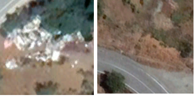
Figure 1: Garbage/Not garbage

Each 200x200 image maps onto a land area of around 20x20m area, with one pixel representing around 10x10cm.

3.3 Data Augmentation

Labelled satellite imagery for ML projects of this sort is laborious to collect in large enough quantities to produce accurate and robust models on their own [31]. Studies have frequently relied on image augmentation to enlarge the dataset whilst preserving the labelling characteristics of the images. Section 2.8 reviewed methods of increasing an image set set via image augmentation.

The geometric augmentations most likely to offer improvement according to [27] were applied as follows (inclusive of the original image):

• cropping: each suitable garbage labelled image and their non-garbage counterpart was subject to the cropping method described in the previous section.

• rotating: each image was rotated by 90, 180, and 270 degrees.

• flipping: each image was flipped horizontally and vertically.

The most promising photometric technique seemed likely to be sharpening, which can improve and enhance edge-detection capabilities, as outlined in [10]. The images were all subjected to a sharpening “kernel” filter.

By combining these augmentation approaches in various ways several datasets were created, ranging from 100 images for the baseline set up to 2,400 images for a pipelined dataset combining all of the techniques above.

3.4 Machine Learning

Once suitably augmented sets of data were obtained, the ML process was carried out as follows:

• choose model instance to go forward with

• tune hyperparameters

• run model against each augmented dataset

• run model against pipelined datasets

• evaluate the results

This iterative process of tuning hyperparameters, training on augmented datasets, combining them in pipelined datasets, and evaluating the results helped in improving the model’s performance and ability to handle novel scenarios.

3.4.1 Choosing the model

Only convolutional neural network (CNN) models were considered for the actual machine learning, as these have been found to be most effective for the sort of problem addressed by this study [32], as explored in section 2.3.

There are many possible CNN models to choose from. It was decided to evaluate a range of those that had been successfully applied to image classification tasks, including several winners of the ImageNet Large Scale Visual Recognition Challenge (ILSVRC) [33]. The process was to apply each candidate model to the baseline (unaugmented) and compare the relative performance of the model, using the metrics described in section 3.5. [5] and [32] suggest that Residual Network model might be most effective when applied to this dataset, which proved to be the case. The results section 4.1 summarises the outcome of this model selection process, including a list of the candidate models evaluated.

All the models evaluated were pretrained. These have already been trained against an image dataset, in this case the publicly available ImageNet dataset [34]. Whilst not consisting exclusively of satellite imagery (in fact only a small proportion is) it has been found that even models pretrained on non-satellite images have an advantage over those not pretrained at all [22].

3.4.2 Modelling Individual Datasets

The following datasets were modelled to establish the relative effectiveness of each data augmentation technique via the selected model, as determined in the results, section 4.1:

• baseline dataset of 100 samples

• geocropped dataset of 200 samples

• sharpened dataset of 200 samples

• flipped dataset of 300 samples

• rotated dataset of 400 samples

For each such dataset performance metrics were collected, as described in section 3.5. The aim of this was to establish a set of baselines for comparison of the various data augmentation techniques and for later evaluation of improvements (or otherwise) as they were pipelined together.

3.4.3 Modelling Pipelined Datasets

There are numerous ways of combining the individual datasets, and it is only practicable to model a subset of these. For this study, to give a reasonable variation of datasets the following pipelines were modelled:

Table 1: Pipelined Models

Pipeline Label	Description	#Samples
pipeline_1	Add each individual dataset into total dataset (the baseline set added in just the once)	800
pipeline_2	For each sample, rotate the sample, flip the sample, add those 6 samples to total dataset. Then sharpen the sample and rotate and flip that sharpened sample, add those 6 samples to the total dataset	1200
pipeline_3	Perform as per pipeline_2 but also do the same with the cropped dataset, doubling the number of samples	2400

Note that rotation operations multiply each sample by 3 (90°, 180°, 270°) and flipping operations multiply each by 2 (horizontal and vertically flipped) - in each case excluding the original sample (to avoid repeatedly including it in the dataset).

3.5 Statistics Gathered

The research undertaken represents a binary classification problem. The model produced classifies image patches as either containing garbage (the “positive” outcome) or not (the “negative” outcome). This implies that for any attempt to classify a particular image, when compared to the actual classification, there are four possibilities [35]:

1. the classification is “contains garbage” and the image does actually contain garbage: a “true positive” (TP)

2. the classification is “contains garbage” but the image does not actually contain garbage: a “false positive” (FP)

3. the classification is “does not contain garbage” and the image does not actually contain any garbage: a “true negative” (TN)

4. the classification is “does not contain garbage” but the image does actually contain garbage: a “false negative” (FN)

Most of the statistics used to assess the efficacy of a binary classification problem make use these four quantities. The ones used in the study, either directly or buried within another statistic, are detailed below.

Accuracy: the percentage of correctly classified predictions with respect to the entire dataset. This gives a good quick indication of how well the model is performing, especially for balanced datasets. See equation 1 for how it is calculated from the figures referred to previously.

$$\mathrm{Accuracy}=\frac{\mathrm{TP}+\mathrm{TN}}{\mathrm{TP}+\mathrm{TN}+\mathrm{FP}+\mathrm{FN}}$$ (1)

Precision: how well the model predicts positive results. See equation 2.

$$\mathrm{Precision}=\frac{\mathrm{TP}}{\mathrm{TP+FP}}$$ (2)

Recall: the fraction of true positive instances that are correctly identified by the model. See equation 3.

$$\mathrm{Recall}=\frac{\mathrm{TP}}{\mathrm{TP+FN}}$$ (3)

These metrics give valuable insight into how well a model is performing in terms of predictive accuracy, but they do not provide a complete picture [36]. There are various useful ways in which these statistics can be combined to produce a more complete picture.

F-Score: this balances precision and recall by calculating their harmonic mean. See equation 4.

$$\mathrm{FScore}=2\times\frac{{\mathrm{Precision}\times\mathrm{Recall}}}{\mathrm{Precion}+\mathrm{Recall}}$$ (4)

However, it can be seen that with the F-Score the true negative quantity is not taken into account (because neither precision nor recall do so).

MCC A statistic which takes account of all parts of the confusion matrix is the Matthew Correlation Coefficient (MCC)[37]. This measures the correlation between the actual and predicted classes, and yields a value between -1 and 1. An MCC of 1 indicates perfect classification, 0 random performance, and -1 a wholly negative correlation. See equation 5. This takes equal account of all four parts of the confusion matrix, so it is one of the preferred statistics used on this study.

3.6 Frameworks/Tools

The research was conducted using the Weka machine learning toolkit (Waikato Environment for Knowledge Analysis) [38]. This is an extensible Java based toolkit that provides support for data preprocessing, implementations of many popular machine learning algorithms, visualisation tools, results statistic reporting, and much more.

For this research Weka was used in conjunction with DeepLearning4J [39], which provides Java implementations of many deep learning models, including convolutional neural networks. Various popular models are provided, such as AlexNet, LeNet, ResNet and Inception. One especially useful feature is that many of these come as “zoo models” [40] pretrained on several publicly available image datasets, including ImageNet [34]. These pretrained models significantly shorten the training time required for new datasets [22], as detailed in section 2.6.

Both Weka and DeepLearning4j provide programmatic API and command line interfaces. Weka also offers a user friendly GUI with which to supply datasets, invoke models, and visualise the results.

In addition, LAMP was used to provide simple data collection and storage utilities [41]. Data augmentation was implemented using the popular ffmepg [42] graphics and video editing software.

All development and machine learning took place on the Linux Ubuntu 20.04 operating system.

3.7 Limitations

A CNN project requires large and diverse datasets for effective training [10]. This project has been based on a modest baseline set of 100 images. However, data augmentation techniques have boosted the dataset size up to 2400. Nevertheless, additional images added to the baseset would add to the predictive performance and generalisation capabilities of the model.

The images were gathered at a resolution of 1 pixel representing 10x10cm of land coverage. The model might not perform as well against different resolution images. In addition, during the research the same land area was found to have different chromatic characteristics depending on what date satellite images were taken. An area for future exploration is to examine how the developed model performs against images that differ in this way. Possibly a model developed against a grey scale could be more robust against such variability. Converting the images to grey scale and rerunning the tests would be an interesting area for future study.

Many of the images were collected in mountainous wooded areas, which tend to predominate on the island. The effects of this were mitigated to an extent by using an independently collected test dataset from other areas of the island without these characteristics. Nevertheless a larger more diverse dataset would only improve the accuracy and robustness of the model.

It may also be the case that trees obscure some instances of garbage from satellite imagery in the visible spectrums, leading to false negatives. It would be an interesting future study to examine if expanding the image spectrum into the infrared might alleviate this.

4 Results and Discussion

This section evaluates the results of the various experiments: to first choose the best performing model type, then optimise the hyperparameters and finally run the model against the various datasets, both unaugmented and augmented. At each stage statistics such as accuracy, F-Score and MCC were collected (see section 3.5) and used as the basis for comparison.

4.1 Model Selection Results

Table 2 shows the results of evaluating the various models to determine a single candidate to move forward with, as described in section 3.4.1. This shows the accuracy, F-Score and MCC metrics for a run of each model on the 100 image baseline dataset.

Table 2: Model Evaluation

Model	Accuracy	F-Score	MCC
LeNet	53.00	0.53	0.06
VGG	N/A	N/A	N/A
AlexNet	50.00	0.45	0.00
KerasInceptionV3	47.00	0.47	-0.06
Xception	50.00	0.37	0.00
ResNet-50	67.00	0.66	0.36

From this it can be seen that the ResNet-50 implementation gives the best performance against all measures . This is consistent with the results of other satellite based land classification studies, as highlighted in section 2.4. The ResNet-50 model was therefore selected for subsequent steps in the process. This model has 48 convolutional layers, one MaxPool layer, and one average pool layer and a total of of around 23.5 million trainable parameters [44].

4.2 Singly Augmented Datasets

Table 3 summarises the results of applying a single augmentation technique to the baseline dataset and adding the augmented dataset to the baseline; the ResNet-50 algorithm was applied to each of these datasets in turn. The trained model used a mini-batch size of 8 and 5x cross-fold validation as described in [45].

Table 3: Single Augmentation Evaluation

Dataset	#samples	Accuracy	MCC	F-Score
Collected baseline	100	56.00	0.12	0.56
Baseline + Cropped	200	83.50	0.68	0.83
Baseline + Sharpened	200	74.00	0.05	0.74
Baseline + Flipped	300	90.33	0.82	0.90
Baseline + Rotated	400	95.25	0.91	0.95

From this it can be seen that each of the augmentation techniques have yielded significant accuracy improvements over just the baseline dataset. The bigger the augmented dataset the greater the improvement, which is broadly in line with expectations. The flipping and rotating augmentation techniques in particular gave results suggestive of very good performance, with accuracy levels 90 percent and above, with similarly good MCC and F-score metrics.

4.3 Pipeline Augmented Datasets

Table 4 summarises the results of the various pipelined experiments, as detailed in section 3.4.3. For each dataset the model was evaluated using each of the three validation methods: 5 times cross-fold, 70% split, and using the independent test dataset. A mini-batch size was chosen of 32, which is fairly standard for datasets of this size and represents a good compromise between generalisation capabilities and computational efficiency.

The table shows the accuracy and MCC metrics for each permutation . An average was taken for each measure against the validation methods as a way of combining the results into a single value.

Table 4: mini-batch size = 32

Dataset	#samples	5x cross-fold		70% split		test dataset		Averaged
		Acc	MCC	Acc	MCC	Acc	MCC	Acc	MCC
pipeline 1	800	98.00	0.96	96.70	0.93	79.00	0.60	90.23	0.83
pipeline 2	1200	99.50	0.99	98.60	0.97	75.00	0.49	91.03	0.82
pipeline 3	2400	99.30	0.98	99.30	0.99	76.0	0.54	91.53	0.84

This table illustrates that in all cases that the trained model performs significantly better than the singly augmented datasets in their ability to correctly classify an image as containing/not containing garbage. They do so with greater than 98% accuracy when validated against the training data, and greater than 75% against the independent test data. This resulted in an overall average accuracy of around 90% and MCC of greater than 0.82. This represents strong performance in terms of classification accuracy and balanced predictions.

5 Conclusion

This study sought to investigate two issues:

• What are the most effective machine learning algorithms and techniques for developing a model that can accurately identify and classify small scale garbage dumps in the rural areas of Cyprus from satellite imagery?

• To what extent can data augmentation techniques improve a machine learning model for such small scale satellite image classification?

To answer these questions a baseline dataset of 100 training satellite image patches was collected using Google Earth [26], which matched verified garbage dump locations. For each garbage image a non garbage image from similar neighbouring terrain was collected. These images were correspondingly labelled as either “garbage” or “not garbage”. Several popular convolutional neural network implementations were trained and evaluated on this baseline set, with the ResNet-50 model showing the most promise.

The baseline dataset was then augmented by applying various combinations of sharpening, rotating, flipping, and cropping. This resulted in “pipelines” of 800, 1200 and 2400 sized image sets. The ResNet-50 model, pretrained on the ImageNet dataset[46], was further trained on each pipelined collection of images and the performance of each model evaluated with respect to the others.

Various validation techniques were used to evaluate the accuracy and generalisation capabilities of the models, including cross-fold validation, employing a holdout dataset, and testing against a separate independently collected set of images.

The experiments showed that ResNet-50 provides an effective machine learning model in the detection of garbage dumps. With just the small baseset of 100 images, a model could be trained that correctly predicts around 70% of novel images. When the size of this baseline sets was expanded using data augmentation then the predictive capabilities of the model increased dramatically, correctly classifying images in more than 90% of cases.

5.1 Future Work

Work is continuing in the area by:

• Increasing the quantity and quality of the baseline dataset. In time this will be made publicly available.

• Investigating automatic methods of obtaining appropriate satellite imagery.

• Developing a system that will allow the techniques explored to map the entire rural environment of Cyprus to develop a comprehensive “garbage map”.

References

- [1] M Vrijheid “Health effects of residence near hazardous waste landfill sites: a review of epidemiologic literature.” In Environmental Health Perspectives 108.suppl 1, 2000, pp. 101–112 DOI: 10.1289/ehp.00108s1101
- [2] GP Gabrielides et al. “Man-made garbage pollution on the Mediterranean coastline” Publisher: Elsevier In Marine Pollution Bulletin 23, 1991, pp. 437–441
- [3] Barry Webb, Ben Marshall, Sarah Czarnomski and Nick Tilley “Fly-tipping: Causes, incentives and solutions” In ill Dando Institute of Crime Science University College London, 2006 URL: https://tinyurl.com/deepterra
- [4] Thomas Kinnaman and Don Fullerton “Garbage and Recycling in Communities with Curbside Recycling and Unit-Based Pricing”, 1997, pp. w6021 DOI: 10.3386/w6021
- [5] Anupama Rajkumar, Continental Automotive Kft, Tamas Sziranyi and Andras Majdik “Detecting Landfills Using Multi-Spectral Satellite Images And Deep Learning Methods” In Proceedings from ICLR 2022, 2022
- [6] Maria Roberta Devesa and Antonio Vazquez Brust “Mapping illegal waste dumping sites with neural-network classification of satellite imagery” arXiv, 2021 DOI: 10.48550/ARXIV.2110.08599
- [7] Michael A. Wulder et al. “Current status of Landsat program, science, and applications” In Remote Sensing of Environment 225, 2019, pp. 127–147 DOI: 10.1016/j.rse.2019.02.015
- [8] Qiang Zhao et al. “Progress and trends in the application of Google Earth and Google Earth Engine” Publisher: MDPI In Remote Sensing 13.18, 2021, pp. 3778
- [9] Gourab Patowary, Meenakshi Agarwalla, Sumit Agarwal and Manash Pratim Sarma “A Lightweight CNN Architecture for Land Classification on Satellite Images” In 2020 International Conference on Computational Performance Evaluation (ComPE) Shillong, India: IEEE, 2020, pp. 362–366 DOI: 10.1109/ComPE49325.2020.9200100
- [10] MAA Ghaffar, A McKinstry, T Maul and TT Vu “Data augmentation approaches for satellite image super-resolution” Publisher: Copernicus GmbH In ISPRS Annals of the Photogrammetry, Remote Sensing and Spatial Information Sciences 4, 2019, pp. 47–54
- [11] Connor Shorten and Taghi M Khoshgoftaar “A survey on image data augmentation for deep learning” Publisher: SpringerOpen In Journal of big data 6.1, 2019, pp. 1–48
- [12] Karen Simonyan and Andrew Zisserman “Very deep convolutional networks for large-scale image recognition” In arXiv preprint arXiv:1409.1556, 2014
- [13] Pourya Shamsolmoali et al. “High-dimensional multimedia classification using deep CNN and extended residual units” Publisher: Springer In Multimedia Tools and Applications 78.17, 2019, pp. 23867–23882
- [14] Marco Castelluccio, Giovanni Poggi, Carlo Sansone and Luisa Verdoliva “Land use classification in remote sensing images by convolutional neural networks” In arXiv preprint arXiv:1508.00092, 2015
- [15] Yann LeCun et al. “Backpropagation applied to handwritten zip code recognition” Publisher: MIT Press In Neural computation 1.4, 1989, pp. 541–551
- [16] Yann LeCun, Yoshua Bengio and Geoffrey Hinton “Deep learning” Publisher: Nature Publishing Group UK London In nature 521.7553, 2015, pp. 436–444
- [17] Charu C Charu C. “The Basic Structure of a Convolutional Network” Publisher: Springer In Neural networks and deep learning Springer, 2018, pp. 318–322
- [18] K Fukushima “Neocognitron: a self-organizing neural network model for a mechanism of pattern recognition unaffected by shift in position” In Biological Cybernetics 36.4, 1980, pp. 193–202
- [19] Yann LeCun, Léon Bottou, Yoshua Bengio and Patrick Haffner “Gradient-based learning applied to document recognition” Publisher: IEEE In Proceedings of the IEEE 86.11, 1998, pp. 2278–2324
- [20] Md Zahangir Alom et al. “The history began from alexnet: A comprehensive survey on deep learning approaches” In arXiv preprint arXiv:1803.01164, 2018
- [21] Alejandro Baldominos, Yago Saez and Pedro Isasi “A survey of handwritten character recognition with mnist and emnist” Publisher: MDPI In Applied Sciences 9.15, 2019, pp. 3169
- [22] Jason Yosinski, Jeff Clune, Yoshua Bengio and Hod Lipson “How transferable are features in deep neural networks?” In Advances in neural information processing systems 27, 2014
- [23] United States Geological Survey “USGS Earth Explorer” In Earth Explorer
- [24] European Space Agency “Copernicus Open Access Hub” In Copernicus Open Access Hub URL: https://scihub.copernicus.eu/
- [25] Gerald Forkuor, Kangbeni Dimobe, Idriss Serme and Jerome Ebagnerin Tondoh “Landsat-8 vs. Sentinel-2: examining the added value of sentinel-2’s red-edge bands to land-use and land-cover mapping in Burkina Faso” Publisher: Taylor & Francis In GIScience & remote sensing 55.3, 2018, pp. 331–354
- [26] Google Corp. “Google Earth Engine” In Google Earth Engine URL: https://earthengine.google.com/
- [27] Luke Taylor and Geoff Nitschke “Improving deep learning with generic data augmentation” In 2018 IEEE Symposium Series on Computational Intelligence (SSCI) IEEE, 2018, pp. 1542–1547
- [28] Steven Lang et al. “Wekadeeplearning4j: A deep learning package for weka based on deeplearning4j” Publisher: Elsevier In Knowledge-Based Systems 178, 2019, pp. 48–50
- [29] “Handling imbalanced datasets in machine learning” In Towards Datasience URL: https://towardsdatascience.com/handling-imbalanced-datasets-in-machine-learning-7a0e84220f28
- [30] Markus Skogsmo “A Scalable Approach for Detecting Dumpsites using Automatic Target Recognition with Feature Selection and SVM through Satellite Imagery”, 2020
- [31] Saikat Basu et al. “Deepsat: a learning framework for satellite imagery” In Proceedings of the 23rd SIGSPATIAL international conference on advances in geographic information systems, 2015, pp. 1–10
- [32] MP Vaishnnave, K Suganya Devi and P Srinivasan “A study on deep learning models for satellite imagery” In International Journal of Applied Engineering Research 14.4, 2019, pp. 881–887
- [33] Olga Russakovsky et al. “Imagenet large scale visual recognition challenge” Publisher: Springer In International journal of computer vision 115, 2015, pp. 211–252
- [34] Stanford Vision Labs “ImageNet”, 2020 URL: https://www.image-net.org/
- [35] AC Müller and S Guido “Model evaluation and improvement in Introduction to Machine Learning with Python, 1e (ed. Müller, AC) 262–263” O’Reilly Media, 2017
- [36] David MW Powers “Evaluation: from precision, recall and F-measure to ROC, informedness, markedness and correlation” In arXiv preprint arXiv:2010.16061, 2020
- [37] Boaz Shmueli “Matthews Correlation Coefficient is The Best Classification Metric You’ve Never Heard Of”, 2019 URL: https://towardsdatascience.com/the-best-classification-metric-youve-never-heard-of-the-matthews-correlation-coefficient-3bf50a2f3e9a
- [38] Eibe Frank, Mark A. Hall, and Ian H. Witten “The WEKA Workbench. Online Appendix for ”Data Mining: Practical Machine Learning Tools and Techniques” In The WEKA Workbench. Online Appendix for ”Data Mining: Practical Machine Learning Tools and Techniques Morgan Kaufmann, 2016
- [39] Rahul Raj “Java Deep Learning Cookbook: Train neural networks for classification, NLP, and reinforcement learning using Deeplearning4j” Packt Publishing Ltd, 2019
- [40] Yang Shu et al. “Zoo-tuning: Adaptive transfer from a zoo of models” In International Conference on Machine Learning PMLR, 2021, pp. 9626–9637
- [41] Xiaosheng Yu and Cai Yi “Design and Implementation of the Website Based on PHP & MYSQL” In 2010 International Conference on E-Product E-Service and E-Entertainment IEEE, 2010, pp. 1–4
- [42] FFmpeg team “FFmpeg” URL: https://ffmpeg.org/
- [43] Sepp Hochreiter “The Vanishing Gradient Problem During Learning Recurrent Neural Nets and Problem Solutions” In International Journal of Uncertainty, Fuzziness and Knowledge-Based Systems 06.02, 1998, pp. 107–116 DOI: 10.1142/S0218488598000094
- [44] Kaiming He, Xiangyu Zhang, Shaoqing Ren and Jian Sun “Deep residual learning for image recognition” In Proceedings of the IEEE conference on computer vision and pattern recognition, 2016, pp. 770–778
- [45] Charu C Charu C. “Evaluating with Hold-Out and Cross-Validation” Publisher: Springer In Neural networks and deep learning Springer, 2018, pp. 179–180
- [46] Alex Krizhevsky, Ilya Sutskever and Geoffrey E. Hinton “ImageNet Classification with Deep Convolutional Neural Networks” Place: New York, NY, USA Publisher: Association for Computing Machinery In Commun. ACM 60.6, 2017, pp. 84–90 DOI: 10.1145/3065386