Mapping Global Value Chains at the Product Level

Abstract

Value chain data is crucial to navigate economic disruptions, such as those caused by the COVID-19 pandemic and the war in Ukraine. Yet, despite its importance, publicly available value chain datasets, such as the “World Input-Output Database”, “Inter-Country Input-Output Tables”, “EXIOBASE” or the “EORA”, lack detailed information about products (e.g. Radio Receivers, Telephones, Electrical Capacitors, LCDs, etc.) and rely instead on more aggregate industrial sectors (e.g. Electrical Equipment, Telecommunications). Here, we introduce a method based on machine learning and trade theory to infer product-level value chain relationships from fine-grained international trade data. We apply our method to data summarizing the exports and imports of 300+ world regions (e.g. states in the U.S., prefectures in Japan, etc.) and 1200+ products to infer value chain information implicit in their trade patterns. Furthermore, we use proportional allocation to assign the trade flow between regions and countries. This work provides an approximate method to map value chain data at the product level with a relevant trade flow, that should be of interest to people working in logistics, trade, and sustainable development.

1 Introduction

Value chain data is important to understand the resilience and systemic effects of disruptions, such as natural disasters [16, 1], climate change [7], war [19, 2], and disease [15]. Publicly available value chain data, such as the OECD Inter-Country Input-Output Database [14], the World Input-Output Database [23], EXIOBASE [22], and EORA [11, 10], however, have limited sectoral resolution, and are often disaggregated into a few dozen industries. This high-level of aggregation can be limiting [9, 6] for applications where detailed product or sectoral resolution is needed, such as tracing the environmental impact and social responsibility of suppliers.

On the contrary, international trade data is much more disaggregated, with 5,000+ categories at the “six-digit level” (HS6 [5]) and 1,000+ categories at the “four-digit level” (HS4). Yet, while international trade data is also a go-to dataset for analysts working to understand disruptions, trade data lacks explicit information about value chain relationships. Trade data can tell us that China imports iron ore from Brazil, but it cannot tell us what that iron ore is used for (e.g. cars, iron rods, aircraft, etc.). Nevertheless, trade theory tells us that this data must contain implicit information about value chain relationships. This information should be hidden in a country or region’s specialization patterns and we should be able to extract it by combining trade theory inspired features with machine learning techniques.

The idea of mapping value chains, however, is not new. Several projects have tried to combine input-output tables [12] and trade data in efforts to map global value chains [11, 10, 23, 14]. These efforts use national input-output tables, connecting sectors at the local level with trade data, to estimate the volume of imported inputs used in each sector of an economy. These efforts, however, tend to rely on proportional allocation methods, where imports are distributed among sectors in the same proportion as local inputs. That is, they assume, for instance, that if 20% of the steel produced in a country is used for the production of machinery, then 20% of the steel imported from any country will also be used for the production of machinery. The result is several datasets [11, 10, 23, 14], that while useful and important, could benefit from better sectoral and spatial resolution.

There is consensus that detailed value chain data can be crucial for a number of applications. Consider the disruptions caused by the Evergreen, the massive container ship that in 2021 became stranded in the Suez Canal [4]. By blocking the Suez Canal, the Evergreen impeded the flow of a large number of products between Asia and Europe [13]. Value chain data can also inform questions with geopolitical implications. Often countries prefer to avoid sourcing key components from geopolitical rivals. For instance, they try to organize their value chains in ways that avoid depending on potential enemies for strategic resources, such as fuel and electronics. Moreover, value chain data can be a key input for environmental assessments [22], since it is needed to account for the environmental impact of imported goods. Finally, value chain data can be important to those working on corporate responsibility. For instance, a clothing company may want to have traceability of their inputs to ensure its products are not produced using forced or child labour.

Yet, despite the glaring need for value chain data, there are no detailed publicly available value chain datasets with fine spatial and sectoral resolution. In this paper, we explore the creation of a method to infer value chain relationships from international trade data to create high-resolution maps of global value chains.

Our method exploits the idea that geographies that specialize in the export of a certain product will tend to specialize in the procurement of its inputs. This tendency should be observed twice in trade data: upstream and downstream. The upstream tendency should be expressed in the products imported by a location that specializes in the export of a product. That is, we expect exporters of computers to specialize in the import of LCDs. Similarly, the downstream tendency should be expressed in the products exported by a location specialized in the import of a product. That is, importers of LCDs will tend to specialize in the export of computers. Here we combine both upstream and downstream specialization patterns in a model that we optimize to identify input-output relationships. We apply this model to a dataset summarizing the exports and imports of 300+ world regions (e.g. states in the U.S., prefectures in Japan, etc.) to create a product-level dataset of value chain relationships for 1,200+ products.

Our method, however, is not without its limitations. While it is designed to operate at the product level, it is not perfectly accurate, meaning that it provides some false-positive value chain relationships. Also, it does not provide a full input-output network, but a set of the most likely value chain links for each product. Moreover, our method requires optimizing four different parameters, a process that can be slow and complicated. Despite these limitations, our results show some promise by identifying 100s of value chain links at the product level. This validates the possibility of using international trade data at the regional level to identify value chain relationships.

In the remaining sections of this paper, we provide a detailed description of our data and methods. The structure of the paper is as follows: we begin with a section that discusses the data utilized in our model (section Data). Following this, we introduce some of the essential trade theory concepts that underpin our approach (section Trade Theory). Then we illustrate a model that uses proportional allocation to assign trade flow in a value chain and, consequently, demonstrating that the missing part of the model is the input-output relationship between products (section Conceptual Model). Next, we introduce and explain our “Backward & Forward" method which predicts input-output relationships between products (section Methodology). Furthermore, we use the “Backward & Forward" method to construct a product-level dataset fine-tuned on the OECD Inter-Country Input-Output table [14], and we validate the results obtained. Our findings are expected to contribute significantly to the development of computational methods aimed at constructing global value chain datasets.

2 Data

We leverage fine-grained international data compiled by the Observatory of Economic Complexity [20] (oec.world) spanning from the year 2017 to 2020. This is data on exports and imports at the regional level for 1,226 HS4 level and 5,890 HS6 level unique products. Because of incompatibilities in data reporting (not all countries report regional trade data using the same classification), our sample is limited to 9 countries: Brazil (32 regions), Canada (13 regions), Chile (16 regions), China (31 regions), Japan (41 regions), Mexico (32 regions), Russia (85 regions), Spain (53 regions) and the United States of America (54 regions).

We clean this dataset by removing unknown regions and reexports such as “Reexportação”, “Exterior”, “Mercadoria Nacionalizada” and “Consumo de Bordo” from the data of Brazil, “Unknown” from the data of the USA and “Sin provincia asignada” from the data of Spain. This leaves us with 351 regions.

We then remove small regions that can provide a noisy signal about their exports and imports (a few dollars of exports and imports can drastically change the observed specialization pattern of regions with low trade volumes). After inspecting the distribution of exports and imports (Figure 1), aggregated from 2017 to 2020, we remove regions on the left tails of the exports and imports distribution. These are regions which in these four years imported in total less than 100 million USD and exported in total less than 1 billion USD. After removing these 44 regions we are left with a final sample of 306 regions.

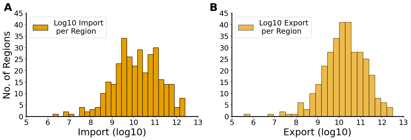
Figure 1: Total import (A) and export (B) distributions across 9 regions from 2017-2020 from the Observatory of Economic Complexity data. Regions include Brazil, Canada, Chile, China, Japan, Mexico, Russia, Spain, and USA.

We note that our data contains export and import information between regions and countries. That is, we know what Barcelona imports from Brazil, or what Sao Paulo imports from Spain, but not what is traded between Barcelona and Sao Paulo.

Finally, we reconcile exports and imports (look for the products to be available in both the exports and import records) and are left with a total of 1,220 HS4 and 5,890 HS6 unique product categories.

In addition, we use the 2021 edition of OECD Inter-Country Input-Output data to fine-tune our model. This is a table containing 45 unique industries based on ISIC Revision 4 (industry, not product categories) for 66 countries. From this data, we produce two tables: OECD specialization and the OECD labeled data. A description of this data can be found at: [14].

3 Trade Theory

Trade theory is the branch of economics studying the patterns in regional and international trade. It has a mathematical tradition of over 200 years, starting with the works of David Ricardo [18]. In this paper, we use trade theory to create some of the basic features for our model.

A key concept in trade theory is the idea of comparative advantage. A location is said to have comparative advantage in the products that it is specialized in. Trade theory tells us that comparative advantages should tell us about the factors that an economy is well endowed with. For instance, we expect economies endowed with vast maritime resources to specialize in the exports of fish and landlocked mountainous economies to specialize in the exports of minerals.

In today’s globalized economy, however, where intermediate inputs are highly mobile, economies often specialize in processes that are not necessarily pinned down by the presence of natural resources but by the availability of knowledge [8]. That is, countries that export cars or furniture do not do so because they are endowed with vast reserves of iron or lumber (they can source these from global markets). This means that countries and regions will tend to import some of the inputs they need to produce the outputs they export. Thus, we should be able to observe value chains implicitly, albeit imperfectly, in international trade flows.

Estimating comparative advantages in practice, however, can be challenging because countries and products can vary greatly in size. Trade theory scholars use indicators of Revealed Comparative Advantage (RCA) [3] (also known as the Location Quotient in urban economics), to measure the level of specialization of a location in a product.

Formally, the Revealed Comparative Advantage of a location in an activity (e.g. a country or region in a product) is simply the double normalization of the export matrix. That is, the $RCA$ of a location $l$ in a product $p$ is defined as:

$$RCA_{lp} =\frac{X_{lp}}{\sum_{p^{\prime}}X_{lp^{\prime}}}/\frac{\sum_{l^{\prime}}X_{l^{\prime}p}}{\sum_{l^{\prime}p^{\prime}}X_{l^{\prime}p^{\prime}}},$$ (1)

where $X_{lp}$ are the exports of location $l$ in product $p$.

$RCA$ can also be interpreted as the ratio between observed and expected exports. When a location has an RCA larger than 1 in a product, we say that the location is specialized in that product since it exports more than what it is expected for a location of the same size and for a product with the same global market.

Going forward, we define two versions of $RCA$. An export $RCA^{export}$, as defined in equation 1, and an import $RCA^{import}$ defined in the same manner, but where $X_{lp}$ represents the imports of location $l$ in product $p$. The $RCA^{import}$ should tell us about the product that a region imports too much. Our hypothesis is that by exploiting specialization patterns across multiple geographies we can generate features that when fed in a machine learning model can recover information about global value chains.

4 Conceptual Model

Formally, our goal is to estimate the tensor $X_{r_{1}p_{1}r_{2}p_{2}}$, representing the flow of product $p_{1}$ coming from region $r_{1}$ and used in region $r_{2}$ to produce product $p_{2}$. The data we have available, however, is much more incomplete and represents two aggregates of the aforementioned tensor. These are: $X_{r_{1}p_{1}c_{2}}$ and $X_{c_{1}p_{1}r_{2}}$, which denote, respectively, the exports of region $r_{1}$ of product $p_{1}$ to country $c_{2}$ (where region $r_{2}$ is located) and the imports of region $r_{2}$ of product $p_{1}$ coming from country $c_{1}$ (where region $r_{1}$ is located).

We estimate $X_{r_{1}p_{1}r_{2}p_{2}}$ using the following proportional allocation model:

$$X_{r_{1}p_{1}r_{2}p_{2}}=\frac{X_{r_{1}p_{1}c_{2}}}{\sum_{r_{1}}X_{r_{1}p_{1}c_{2}}}\underbrace{L_{p_{1}p_{2}}}_{\text{unknown}}\frac{X_{r_{2}p_{2}}}{\sum_{p_{2}}X_{r_{2}p_{2}}}X_{c_{1}p_{1}r_{2}},$$ (2)

where the first fraction represents the share of exports in region $r_{1}$ of product $p_{1}$ to country $c_{2}$ over the total exports of product $p_{1}$ to country $c_{2}$. This term shows us how specialized in export of product $p_{1}$ to country $c_{2}$ is the region $r_{1}$ in comparison with all the other regions from its country $c_{1}$. $L_{p_{1}p_{2}}$ is a binary tensor where 1 represents a positive input-output relationship between the products $p_{1}$ and $p_{2}$ (Figure 2). However, from our available data the $L$ matrix is not known. The second fraction is the share of export of product $p_{2}$ in region $r_{2}$ over all the exports of region $r_{2}$. This term shows us how specialized the region $r_{2}$ is in the export of the product $p_{2}$. Lastly, $X_{c_{1}p_{1}r_{2}}$ is the trade flow in exports of product $p_{1}$ from country $c_{1}$ to region $r_{2}$.

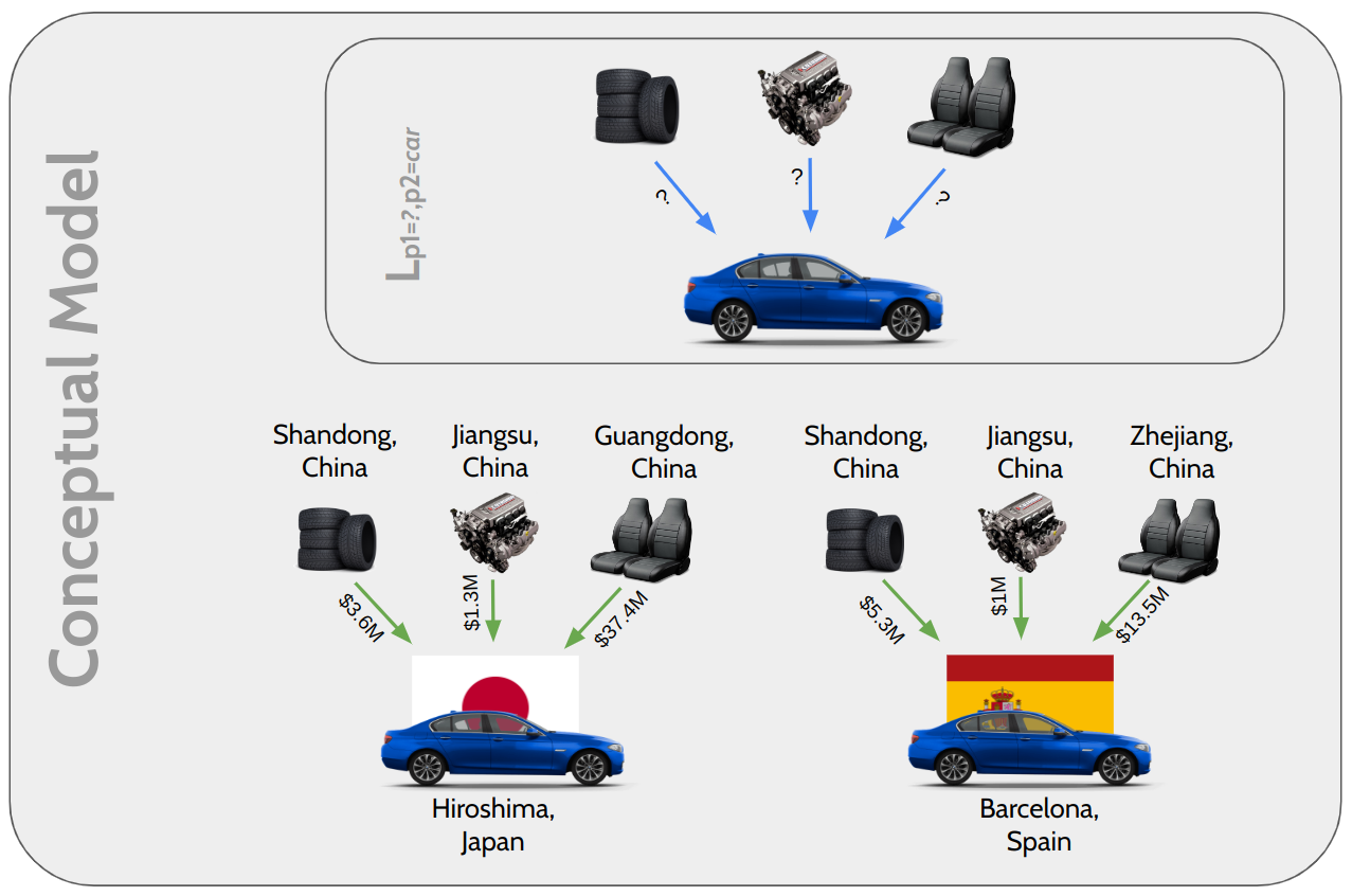
Figure 2: The Conceptual Model utilizes the input-output relationship produced by the L term and further quantifies the trade flow between two regions. In this figure, the term L provides the information that Cars need Rubber Tires, Engine Parts and Seats for their production. Whereas, the Conceptual Model uses the input-output information to quantify the exports of Rubber Tires, Engine Parts and Seats from Hiroshima to Barcelona which would be used for Barcelona’s local production of Cars.

Consider the example where we want to find the trade flow of engine parts from Jiangsu Province (region in China) to Barcelona (region in Spain). In this example, $\frac{X_{r_{1}p_{1}c_{2}}}{\sum_{r_{1}}X_{r_{1}p_{1}c_{2}}}$ is the share of Jiangsu in the export of Chinese engine parts to Spain. The $L_{p_{1}p_{2}}\frac{X_{r_{2}p_{2}}}{\sum_{p_{2}}X_{r_{2}p_{2}}}$ term would be the predicted output products of engine parts (ex. cars, trucks, boats etc.) multiplied by the share of export of Barcelona of those products. And $X_{c_{1}p_{1}r_{2}}$ would be the imports of Chinese engine parts by Barcelona. By multiplying the previously mentioned terms we should be able to estimate how much Barcelona spends in imports of engine parts from Jiangsu Province for i local production of ex. cars, trucks, and boats.

The data that we have access to provides the information to calculate the term $X_{c_{1}p_{1}r_{2}}$, and the two fractions: $\frac{X_{r_{1}p_{1}c_{2}}}{\sum_{r_{1}}X_{r_{1}p_{1}c_{2}}}$ and $\frac{X_{r_{2}p_{2}}}{\sum_{p_{2}}X_{r_{2}p_{2}}}$. However, the terms ${X_{r_{1}p_{1}r_{2}p_{2}}}$ and $L_{p_{1}p_{2}}$ are unknown.
In the next chapter, Methodology, we present a method to calculate the binary matrix $L_{p_{1}p_{2}}$.

5 Methodology

5.1 Backward & Forward Method

A link in a value chain can be traversed in two directions: a downstream or forward direction (from sunflower seeds to sunflower oil) and an upstream or backward direction (from sunflower oil to sunflower seeds) [21].

To estimate the term $L_{p_{1}p_{2}}$ from Equation 2 we introduce the “Backward & Forward” method. The “Backward & Forward” method combines the “Forward” and the “Backward” approaches inspired by the downstream and upstream value chain flows.

In the “Forward” approach, we start by selecting an import product $C$ and then we select the regions that import a disproportionately large number of product $C$ (using an $RCA^{import}$ measure). This provides us with a list of locations sorted by import RCA (e.g. Alabama, Aguascalientes, etc.), which are places that import “too much” of that product. We then look at the export specialization of these regions. The result is a matrix of the exports of the locations that import “too much” of a product. We then attempt to learn the outputs associated with the import from the over-expressed exports of these locations.

In the “Backward” approach we first select an export product $P$ and then identify the locations that export a disproportionately large number of that product. We then analyse what these locations specialize in, in terms of imports. The result is a matrix of the imports of the locations that export “too much” of the selected product. We then attempt to learn the inputs of that product using the values from the matrix.

Every product has an input but not every product has an output. For example, “Rolled Tobacco” (aka cigarette) is a final product that goes directly into consumption. While, raw materials as "Iron Ore" still need excavation machines to be extracted and transported. For that reason, we identify inputs of every product by first applying the “Backward” and then validating with the “Forward” approach. We call this the “Backward & Forward” method.

In pseudo-code (Algorithm 1), we identify the inputs of all of our products $P$ by fixing a product $P_{i}$ ($P_{i}\in P$ where $1\leq i\leq No.\_of\_products$) and apply the “Backward” approach first (“get_n_input_candidates()”). This gives us the top n input candidates $C$ ($C_{j}\in C$ where $1\leq j\leq n$) for the input $P_{i}$. If we find $P_{i}$ as an input to itself in $C$ we remove it (“drop()”). Then, for each $C_{j}$, we apply the “Forward” approach (“get_n_output_candidates()”) to identify the outputs of $C_{j}$, called $T$. We then look for product $P_{i}$ in the outputs ($T$) of $C$. If we find $P_{i}$ in $T$, we take the rank (“getRank()”) of $P_{i}$ in $T$ and add it to the rank of $C_{j}$ in the inputs of $P_{i}$. And if we do not find $P_{i}$ in $T$, then we take the worst ranking which is the one of the last $P_{n}$ candidate product and add plus one, and add it to the rank of $C_{j}$ in the inputs of $P_{i}$. This technique updates (“updateRank()”) the initial ordering of $C_{j}$ as an input of $P_{i}$. We then order the products by ascending order (“order_by_rank_ascending()”). This makes “2” the minimum and best possible rank meaning that $C_{j}$ was the first candidate (rank 1) as an input to $P_{i}$ and $P_{i}$ was the first candidate (rank 1) as an output to $C_{j}$.
By merging both the “Backward” and then the “Forward” method, we are able to first identify and then validate and update our input-product results.

Algorithm 1 Backward & Forward Algorithm

for every $P_{i}\in P$ do

    

    $C\leftarrow get\_n\_input\_candidates(P_{i})$ $\triangleright$ Backward

    if $P_{i}$ in $C$ then

         $C.drop(P_{i})$

    end if

    for every $C_{j}\in C$ do

         

         $T\leftarrow get\_n\_output\_candidates(C_{j})$ $\triangleright$ Forward

         if $P_{i}\in T$ then

             $value\leftarrow T.getRank(P_{i})$

         else

             $value\leftarrow T.getRank(T_{n})+1$

         end if

         $old\_rank\leftarrow C.getRank(C_{j})$

         $new\_rank\leftarrow old\_rank+value$

         $C.updateRank(C_{j},new\_rank)$ $\triangleright$ Update ranking

    end for

    $result\leftarrow C.order\_by\_rank\_ascending()$

end for

5.2 Fine-tuning

In the “Backward & Forward” method we come across a few parameters that we need to optimize: two parameters in the “Backward” and two in the “Forward” approach.

In the “Backward” approach we have the specialization of exporters threshold ($rca\_locations\_1$). This is the minimum $RCA^{export}$ a location needs to have to be considered specialized in the export of a certain product. Then, we have the import specialization of industries/products threshold ($rca\_industries\_1$). This helps us rank the input candidates by counting how many of the specialized export locations, that we identified before, are also specialized in the import of the input candidate.

Similarly, in the “Forward” approach, we have the specialization of importers threshold ($rca\_locations\_2$). This is the minimum $RCA^{import}$ a location needs to have to be considered specialized in the import of a certain product. Then, we have the export specialization of industries/products threshold ($rca\_industries\_2$). This helps us rank the output candidates by counting how many of the specialized import locations, that we identified before, are also specialized in the export of the output candidate.

To optimize the parameters $rca\_locations\_1$, $rca\_industries\_1$, $rca\_locations\_2$ and $rca\_industries\_2$ we feed the OECD ICIO specialization data to the “Backward & Forward" Model. Then we use the OECD labeled data to evaluate the model.

Considering the nature of our value chain problem, the full result would be a sparse matrix with many 0s and very few 1s. Meaning that a big part of all the possible product pairs’ input-output relationships (1488400 HS4 and 34692100 HS6 products) will be false and very few will be true. The model should prioritize identifying the true relationships. For this reason, we use precision as an evaluation metric which tells us how many of our predicted input-output relationships are correctly classified [17].

To optimize the parameters we perform a grid search. Looking at the distributions of RCAs in Figure 3, we test all the combinations of $rca\_locations\_1$, $rca\_industries\_1$, $rca\_locations\_2$ and $rca\_industries\_2$ assigned with a value in the interval of $\left[1,6\right[$ with step of 0.5. For every combination, we calculate the corresponding precision.

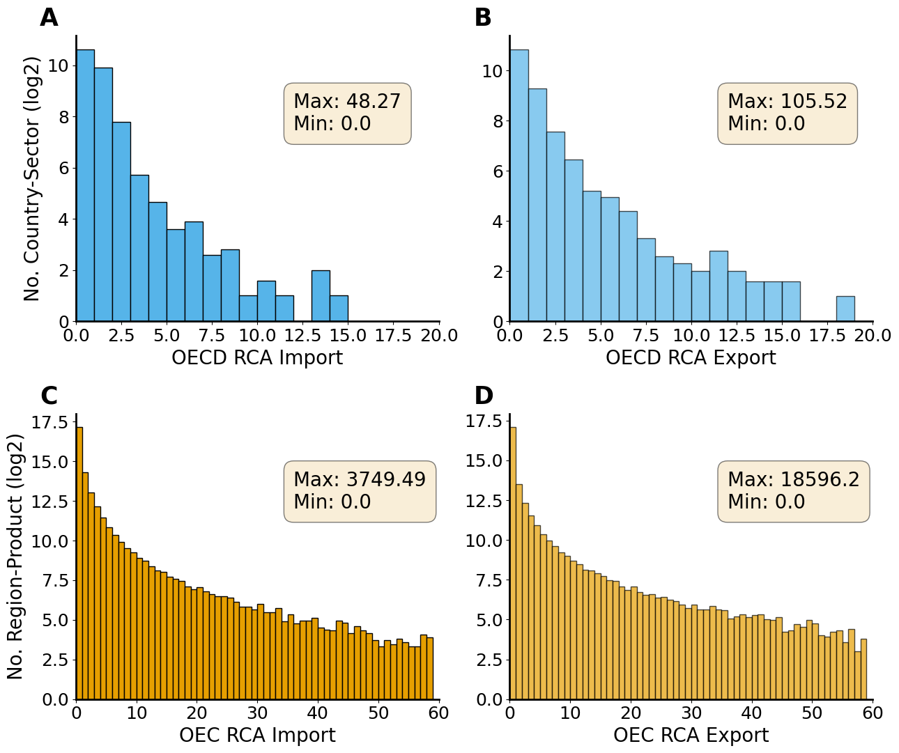
Figure 3: Total OECD RCA import (A), OECD RCA export (B), OEC RCA import (C) and OEC RCA export (D) distribution across all the product-region in the case of the OEC and the sector-country pairs in the case of OECD data between 2017 and 2020.

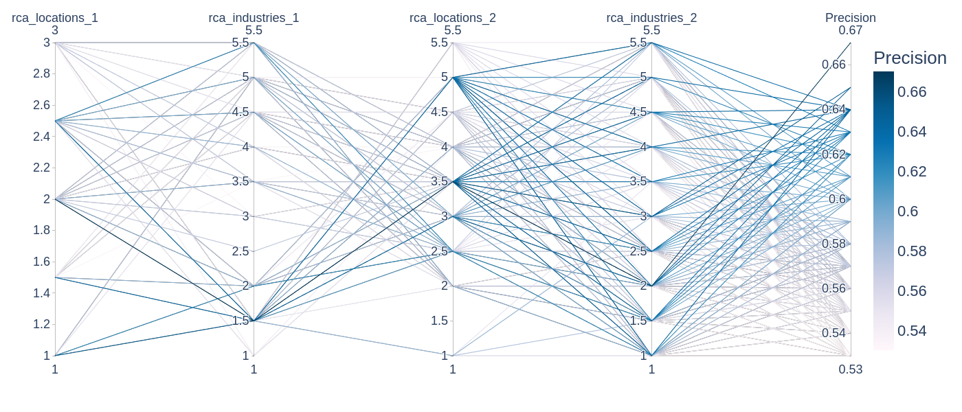
Figure 4: Parallel coordinate plot showing the 500 highest in precision combinations of the parameters: rca_location_1, rca_industries_1, rca_location_2 and rca_industries_2. The precision values are rounded to two decimals.

The Figure 4 shows the 500 combinations that achieved the highest precision. The best precision is 0.67 with the $rca\_locations\_1=2$, $rca\_industries\_1=1.5$, $rca\_locations\_2=3.5$ and $rca\_industries\_2=2$.

In Figure 5 we can see the value chain network produced by the “Backward & Forward” model using the best parameters. With the OECD labeled data, we are able to colour the correct links with green and the incorrect ones with red. There are 84 true-positive and 48 false-positive input-output links.

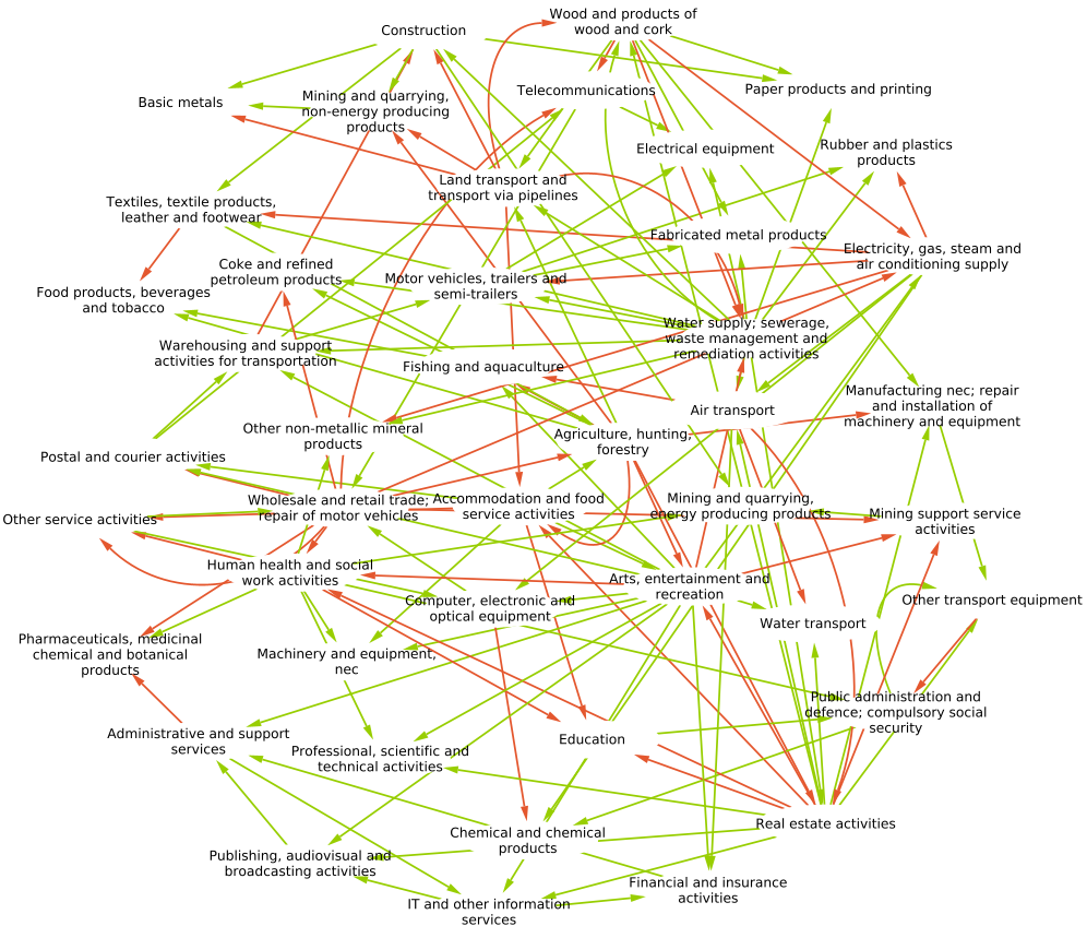
Figure 5: Resultant value chain network that consists of nodes representing industries and directed edges representing the input-output connections between the industries. The edges are labelled using the OECD labelled data, with red edges indicating misclassified links and green edges indicating correctly identified inputs by the Backward & Forward method.

6 Results

To produce our final results, we apply the “Forward & Backward” method on every traded product to get the 3 top input candidates. For the model’s parameters we use $rca\_locations\_1=2$, $rca\_industries\_1=1.5$, $rca\_locations\_2=3.5$ and $rca\_industries\_2=2$.

Our initial application of the “Backward & Forward” method focuses on 1200 HS4 products. In Figure 6 we see part of the value chain networks produced by the “Backward & Forward” method using HS4 trade data. These examples were validated manually. Red edges represent false positive, while the green edges are true positive value chain relationships.
Examples of accurately identified products are the inputs of “Cars” and “Delivery Trucks” where for both we get “Motor vehicle parts and accessories (8701 to 8705)”, “Electrical Lighting and Signaling Equipment” and “Padlocks”. Other examples are “Telephones” and “Computers” where the inputs for the former are “LCDs”, “Electrical Parts” and “Integrated Circuits”, and for the latter are “Photographic Chemicals”, “Machines and apparatus of a kind used solely or principally for the manufacture of semiconductor boules or wafers, semiconductor devices, electronic integrated circuits or flat panel displays” and “Other Measuring Instruments”. The other correct results we can see in the figure are for the products “Processed Tobacco” and “Integrated Circuits”.
However, we also see some false positive results in Figure 6. In the example of “Electrical Ignitions” the model incorrectly predicts as inputs “Audio and Video Recording Accessories” and “Knit Gloves” while it correctly predicts “Electromagnets”. Other examples where our model is able to identify only one correct input are “Military Weapons”, “Jewellery” and “Pig Iron”.

Output	Input	Input	Input
Cars	Motor vehicles parts	Electrical Lighting/Signalling	Padlocks
Delivery Trucks	Motor vehicles parts	Electrical Lighting/Signalling	Padlocks
Processed Tobacco	Raw Tobacco	Scented Mixtures	Conveyor Belt Textiles
Integrated Circuits	Chemicals for Electronics	Apparatus for semiconductors	Oscilloscopes
Telephones	Integrated Circuits	Electrical Parts	LCDs
Computers	Photographic Chemicals	Other Measuring Instruments	Apparatus for semiconductors
Petroleum Coke	Refined Petroleum	Surveying Equipment	Reaction and Catalytic Products
Refined Petroleum	Other Iron Products	Electric Generating Sets	Cranes
Electrical Ignitions	Knit Gloves	Electromagnets	Audio-Video Recording
Leather of Animals	Leather Machinery	Synthetic Tanning Extracts	Synth. Filam. Yarn Woven Fabric
Synthetic Fabrics	Looms	Unprocessed Artificial Staple Fibers	Semi chemical Woodpulp
Corn	Mill Machinery	Iron Radiators	Harvesting Machinery
Jewellery	Cars	Hard Liquor	Pearl Products
Pig Iron	Electric Furnaces	Tensile Testing Machines	Soldering/welding Machinery
Plane, Helicop., Spacecraft	Aircraft Parts	Parts of aircraft and spacecraft	Other Furniture
Military Weapons	Other Furniture	Explosive Ammunition	Light Fixtures

Table 1: HS4 examples produced by the Backward & Forward method where the green cell represents a correctly predicted input candidate and red incorrectly. For readability, some of the product names have been shortened.

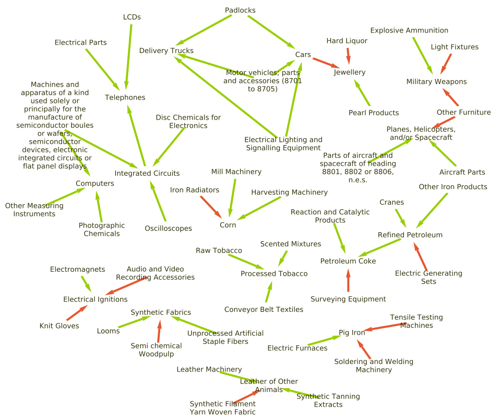
Figure 6: A subset of our resultant value chain network that consists of nodes representing HS4 products and directed edges representing the input-output connections between the products. The edges are manually labelled, with red edges indicating misclassified links and green edges indicating correctly identified inputs.

Next, our method is applied to a more granular product classification, namely the HS6, which consists of over 5000+ distinct products. In Figure 7 we see examples of the value chain networks produced by the “Backward & Forward” method using HS6 products. Notably, our method accurately identifies the inputs of “Medium Sized Cars”, “Cigarettes containing tobacco”, “Telephones for cellular networks or for other wireless networks” and “Electronic integrated circuits: processors and controllers, whether or not combined with memories, converters, logic circuits, amplifiers, clock and timing circuits, or other circuits” even at this more granular level of product classification.
The model predicted false positive results for “Helicopters of an unladen weight $<$ 2,000 kg” with the inputs “Rowing boats, canoes, pleasure boats except sail/powe” and “Almonds,fresh or dried, shelled”. The product “Pig iron, non-alloy, $<$0.5% phosphorus” has no correct inputs.

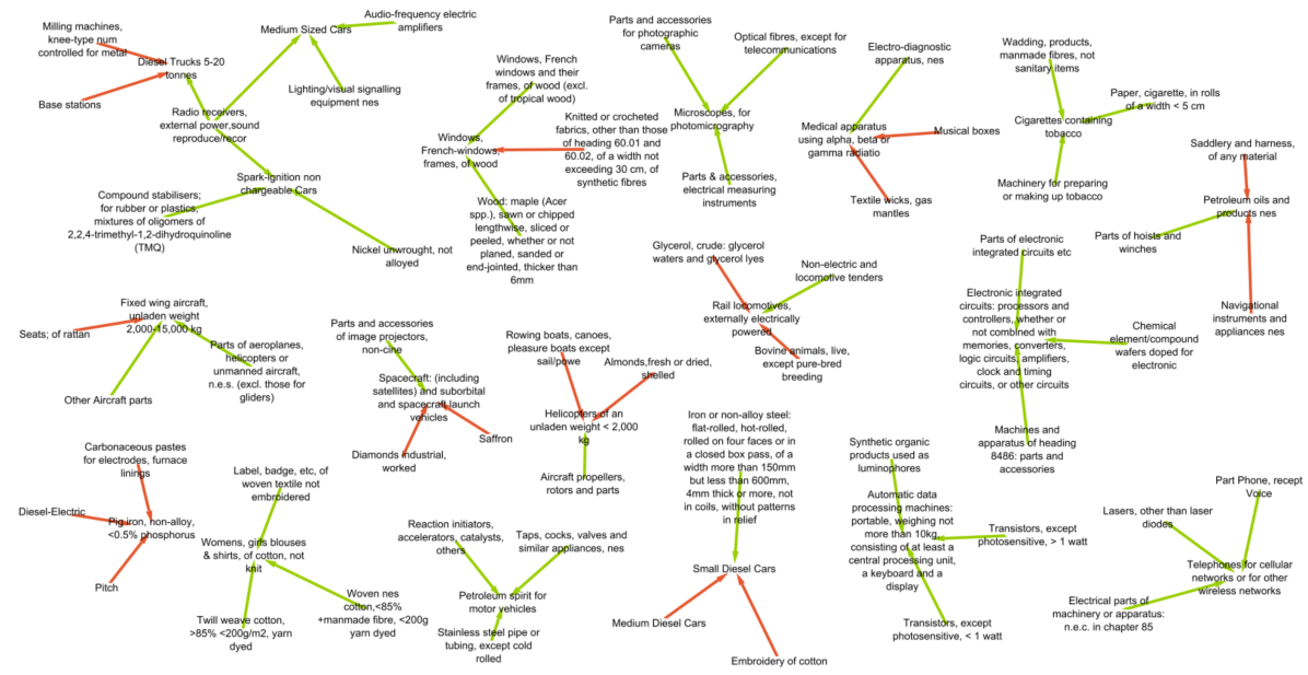
Figure 7: A subset of our resultant value chain network that consists of nodes representing HS6 products and directed edges representing the input-output connections between the products. The edges are manually labelled, with red edges indicating misclassified links and green edges indicating correctly identified inputs.

6.1 Validation

To evaluate our estimation of the $L_{p_{1}p_{2}}$ term using the “Backward & Forward” method we compare it with a baseline model which randomly picks out three inputs for each product. Due to the lack of a benchmark to validate the trade data results produced by the “Backward & Forward”, we perform a random sampling of 50 products. Then we manually label the identified inputs of those 50 products.

Figure 8 shows the percentage of outputs having at least one, two and three inputs correctly identified. On the y-axis we have the different models: “Baseline Model” (B) and “Backward & Forward Model” (BF) using the HS6 and HS4 product classifications. Furthermore, we test the case where the output products are only part of the “Machinery" group (M). In the Figure 8 we see that our model is able to identify at least one of the inputs for 70% of the 50 HS4 products coming from the group of “Machinery", whereas the baseline is able to identify only 30%. We can see similar performance between the “Baseline" and the “Backward & Forward Model" in the other cases as well. With this, we conclude that the “Backward & Forward" performs significantly better than the “Baseline Model".

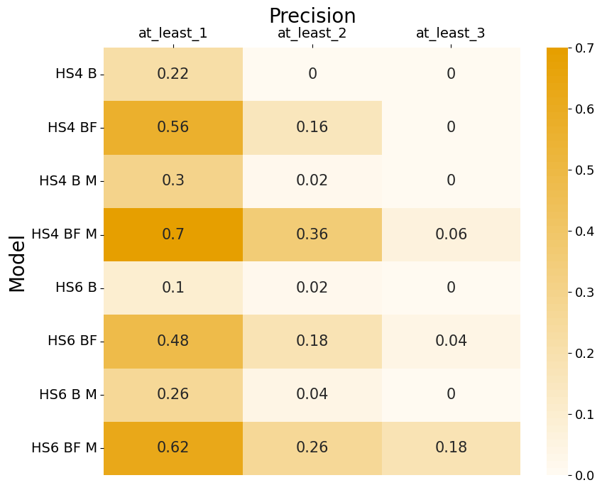
Figure 8: Heatmap showing our manually validated results by randomly sampling 50 input-output relationships. The values represent the percentage of the 50 examples that in the first column had at least one correctly identified input product, in the second column at least two and in the third column all of the input products identified correctly by the Backward & Forward model using the different types of models (B – Baseline and BF – Backward & Forward) and data (HS4, HS6 and M – Machinery products) specified on the y-axis.

7 Conclusion

Here we presented a first attempt to learn value chain relationships and estimate trade flows from trade data, by combining concepts from trade theory with machine learning techniques. While data on global value chains is notoriously aggregated, the "Forward & Backward" method offers a promising solution for mapping global value chains at the product level.

However, it is important to acknowledge that our method is not perfect. Although it operates at the product level, it may provide some false-positive value chain relationships, and it does not offer a complete input-output network. Additionally, optimizing the four different parameters of our method can be a slow and complicated process.

Despite these limitations, the “Backward & Forward” method outperforms the random baseline, identifying at least one correct input for more than 40% of the data, which is more than twice as much as the capabilities of a random baseline model. We also demonstrate that the method identifies correctly three inputs for complex products such as cars, integrated circuits, computers, and telephones. This validates the possibility of using international trade data at the regional level to identify value chain relationships.

Increasing the accuracy of the “Backward & Forward” method represents an interesting avenue for future research. One approach is by fine-tuning the model with input-output tables that have a higher sectoral and geographical resolution than the present OECD ICIO data. Another approach is to expand the regional trade data by linking product codes with different classifications (e.g. SITC, CPC, SIC, GTAP) to HS. Lastly, extending the model to predict more than three inputs per output would bring us closer to obtaining a complete value chain network.

We thank Ron Boschma, the participants of the International PhD course in Economic Geography, Utrecht 2022, and the members of the Center for Collective Learning for their valuable input. This project was supported by the National Institute of Standards and Technology, ANR-19-PI3A-0004 and LearnData ERA Chair Grant agreement ID: 101086712.

8 Appendix

8.1 OEC Trade Data Manipulation

We use regional trade data from the Observatory of Economic Complexity (oec.world) for our results.
We combine the data for the 306 regions into a table containing as columns: “geography”– name of the region, “product”– HS4 product name, “value_imp”– the import trade value, “value_exp”– the export trade value, “geography_exp”– total exports of the region, “geography_imp”– total imports of the region, “product_exp”– total exports of the product, “product_imp”– total imports of the product, and two classical measures of specialization “rca_exp” and “rca_imp.”

$$RCA_{exp}=\frac{\frac{value\_exp}{geography\_exp}}{\frac{product\_exp}{sum(value\_exp)}},$$

$$RCA_{imp}=\frac{\frac{value\_imp}{geography\_imp}}{\frac{product\_imp}{sum(value\_imp)}}$$

In the Table 2 we can see the final look of our trade data.

	geography	value_imp	product	geography_imp	product_imp	rca_imp	value_exp	geography_exp	product_exp	rca_exp
0	Ciudad de México	5882480.0	Other Vegetable Products	4.101108e+11	6.901484e+10	0.011240	1775336.0	3.633443e+11	1.509038e+09	1.057660
1	Guanajuato	2468431.0	Other Vegetable Products	3.754898e+10	6.901484e+10	0.051516	4320249.0	3.447602e+10	1.509038e+09	27.125367
2	Jalisco	9451035.0	Other Vegetable Products	9.338915e+10	6.901484e+10	0.079306	34593964.0	6.327343e+10	1.509038e+09	118.348546
3	Estado de México	508352.0	Other Vegetable Products	6.436369e+10	6.901484e+10	0.006189	2616971.0	3.181877e+10	1.509038e+09	17.803261
4	Nuevo León	3813095.0	Other Vegetable Products	1.256306e+11	6.901484e+10	0.023785	51550913.0	1.262054e+11	1.509038e+09	88.418374
…	…	…	…	…	…	…	…	…	…	…
196117	Metropolitana De Santiago	6178.30	Titanium Ore	2.233049e+11	1.166828e+11	0.000013	551658.00	2.108547e+11	2.649914e+08	3.225070
196118	Metropolitana De Santiago	172.95	Granulated Slag	2.233049e+11	3.079868e+08	0.000136	335812.32	2.108547e+11	4.000072e+10	0.013006
196119	Metropolitana De Santiago	848039.05	Prepared Explosives	2.233049e+11	1.898840e+09	0.108167	38389897.04	2.108547e+11	1.352253e+09	43.980460
196120	Metropolitana De Santiago	483473.53	Railroad Ties	2.233049e+11	4.331550e+09	0.027033	191154.59	2.108547e+11	7.041212e+08	0.420570
196121	Metropolitana De Santiago	274.74	Scrap Aluminium	2.233049e+11	5.365896e+10	0.000001	98316711.65	2.108547e+11	1.346654e+11	1.131025

Table 2: OEC Final Trade Data Table

8.2 OECD Data Manipulation

To fine-tune our “Backward and Forward” method we use the OECD Inter-Country Input-Output (ICIO) Tables. Here, we work with the intermediate use at basic prices data from 2016, 2017 and 2018, and we merge them by summing up the trade flows. To clean the data, we merge the data of China “CN1”, “CN2” and “CHN” into "CHN". We do the same to the Mexico data, “MX1", “MX2" and “MEX" into “MEX". We also remove the country “ROW" which represents “Rest of the World" as it can introduce noise to the model.

Concerning the industries, we remove the industry 97T98 “Activities of households as employers; undifferentiated goods- and services-producing activities of households for own use" as it has not been traded.
We end up with a matrix of 2904x2904 industries-country pairs (44x66).
Moreover, we put the trade flow of reexports, export from and to the same country, to 0.

First, we start by creating the tunning table. For every country-industry pair, we put the country code in "geography" column and the product code in "product" column. Then in “value_imp" column we sum over the columns and for the “value_exp" we sum over the rows. Next, we calculate the “geography_exp" by grouping over “geography" and summing up the “value_exp", and “product_exp" by grouping over "product" and summing up the “value_exp". We do the same to calculate the “geography_imp", by grouping over “geography" and summing up the “value_imp", and “product_imp" by grouping over “product" and summing up the “value_imp". As we did for the Trade Data, using the formula $\frac{\frac{value\_exp}{geography\_exp}}{\frac{product\_exp}{sum(value_{e}xp)}}$ we calculate “rca_exp". And we use the formula $\frac{\frac{value\_imp}{geography\_imp}}{\frac{product\_imp}{sum(value_{i}mp)}}$ to calculate “rca_imp".
Table 3 shows the final look of the training data.

	value_imp	geography	product	geography_imp	product_imp	rca_imp	value_exp	geography_exp	product_exp	rca_exp
0	11619.407384	AUS	01T02	353818.854850	835032.99528	1.440590	22935.551244	595965.513523	768630.020805	1.834052
1	4840.318308	AUT	01T02	321604.777528	835032.99528	0.660220	2193.216844	349635.801449	768630.020805	0.298944
2	7049.627146	BEL	01T02	526307.471482	835032.99528	0.587576	4927.290870	532869.434581	768630.020805	0.440667
3	27917.032198	CAN	01T02	876406.697376	835032.99528	1.397336	37023.829481	909091.443344	768630.020805	1.940874
4	3671.147871	CHL	01T02	93649.791607	835032.99528	1.719620	7221.641047	174677.439401	768630.020805	1.970256
…	…	…	…	…	…	…	…	…	…	…
2899	521.915500	ZAF	94T96	147558.428838	253890.016018	0.510307	1.420904	158225.011733	15681.17867	0.020977
2900	2375.654280	TWN	94T96	576254.654859	253890.016018	0.594791	93.548425	693550.512370	15681.17867	0.315080
2901	4563.273980	THA	94T96	473645.715393	253890.016018	1.390011	0.000000	396945.386345	15681.17867	0.000000
2902	41.091241	TUN	94T96	29409.824719	253890.016018	0.201582	6.295216	21764.013076	15681.17867	0.675669
2903	1962.493248	VNM	94T96	502262.634668	253890.016018	0.563732	1.248322	345511.049333	15681.17867	0.008440

Table 3: Final OECD Table

Then, we move on to creating the labeled data. For this, we take the initial table (country-industry x country-industry pairs and we sum over the industries so that we get a matrix of 44x44 industries with their corresponding trade flows.
Afterwards, we apply the trade intensity formula for every input-output industry and get the Table 4. Trade Intensity (TI). TI index, according to Yamazawa[24], is used to determine whether the value of trade between two countries is greater or smaller than would be expected on the basis of their importance in world trade. It is defined as the share of one country’s exports going to a partner divided by the share of world exports going to the partner.
In our situation we will be using the TI between products (industries).

We calculate it as:

$$TI_{pp^{\prime}}=\frac{X_{pp^{\prime}}/\sum_{p^{\prime}}X_{pp^{\prime}}}{\sum_{p}X_{pp^{\prime}}/\sum_{pp^{\prime}}X_{pp^{\prime}}}$$ (3)

Where $X_{pp^{\prime}}$ and $\sum_{p}X_{pp^{\prime}}$ are the trade flows from industry $p$’s and from all the industries to industry $p^{\prime}$, and where $\sum_{p^{\prime}}X_{pp^{\prime}}$ and $\sum_{pp^{\prime}}X_{pp^{\prime}}$ are industry $p$’s total exports and total export of all industries respectively. An index of more (less) than one indicates a trade flow that is larger (smaller) than expected between the two products (industries).

Then, we binarize the matrix by applying $\begin{dcases}1,&\text{if }TI\geq 1\\ 0,&\text{otherwise}\end{dcases}$.
The labeled data that we get is depicted in Table 4.

When we map the entire input-output network between the industries we get the value chain shown in the Figure 9.

	01T02	03	05T06	07T08	09	…	84	85	86T88	90T93	94T96
01T02	1	1	0	0	0	…	1	1	1	1	1
03	0	1	0	0	0	…	1	1	1	1	1
05T06	0	1	1	1	1	…	1	1	1	1	1
…	…	…	…	…	…	…	…	…	…	…	…
86T88	0	0	0	0	0	…	0	1	1	0	1
90T93	0	0	0	0	0	…	1	1	1	1	1
94T96	0	0	0	0	0	…	0	1	0	0	1

Table 4: Trade Intensity Binary OECD Table

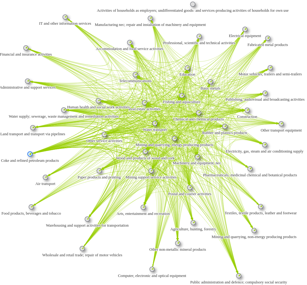
Figure 9: Depicts the full OECD binarized/labeled network that consists of nodes representing sectors and edges representing the input-output connections between the sectors.

References

- [1] Masato Abe and Linghe Ye, ‘Building resilient supply chains against natural disasters: The cases of japan and thailand’, Global Business Review, 14(4), 567–586, (2013).
- [2] Abdelaaziz Ait Ali, Fahd Azaroual, Oumayma Bourhriba, and Uri Dadush, ‘The economic implications of the war in ukraine for africa and morocco’, Policy notes & Policy briefs 1970, Policy Center for the New South, (2022).
- [3] Bela Balassa, ‘Trade liberalisation and “revealed” comparative advantage1’, The Manchester School, 33(2), 99–123, (1965).
- [4] BBC. Suez Canal: Fresh effort to refloat wedged container ship - BBC News, March 2021.
- [5] Peggy Chaplin, ‘An introduction to the harmonized system’, NCJ Int’l L. & Com. Reg., 12, 417, (1987).
- [6] Christian Diem, Andr’as Borsos, Tobias Reisch, J’anos Kert’esz, and Stefan Thurner, ‘Estimating the loss of economic predictability from aggregating firm-level production networks’, Papers 2302.11451, arXiv.org, (February 2023).
- [7] Abhijeet Ghadge, Hendrik Wurtmann, and Stefan Seuring, ‘Managing climate change risks in global supply chains: a review and research agenda’, International Journal of Production Research, 58(1), 44–64, (2020).
- [8] Ricardo Hausmann, César A. Hidalgo, Sebastián Bustos, Michele Coscia, Alexander Simoes, and Muhammed A. Yıldırım, The Atlas of Economic Complexity: Mapping Paths to Prosperity, The MIT Press, 2013.
- [9] Robert C. Johnson, ‘Measuring global value chains’, Annual Review of Economics, 10(1), 207–236, (2018).
- [10] Manfred Lenzen, Keiichiro Kanemoto, Daniel Moran, and Arne Geschke, ‘Mapping the structure of the world economy’, Environmental Science & Technology, 46(15), 8374–8381, (2012). PMID: 22794089.
- [11] Manfred Lenzen, Daniel Moran, Keiichiro Kanemoto, and Arne Geschke, ‘Building eora: A global multi-region input–output database at high country and sector resolution’, Economic Systems Research, 25(1), 20–49, (2013).
- [12] Wassily Leontief, Input-output economics, Oxford University Press, 1986.
- [13] Nik Martin. Suez Canal: One of the biggest trade chokepoints – DW – 03/27/2021, March 2021.
- [14] OECD, ‘Oecd inter-country input-output database’, (2021).
- [15] OECD, Strengthening Economic Resilience Following the COVID-19 Crisis, 2021.
- [16] YoungWon Park, Paul Hong, and James Jungbae Roh, ‘Supply chain lessons from the catastrophic natural disaster in japan’, Business Horizons, 56(1), 75–85, (2013).
- [17] David M. W. Powers, ‘Evaluation: from precision, recall and f-measure to roc, informedness, markedness and correlation’, (2020).
- [18] David Ricardo, ‘From the principles of political economy and taxation’, in Readings in the economics of the division of labor: The classical tradition, 127–130, World Scientific, (2005).
- [19] Michele (ed.) Ruta, ‘The impact of the war in ukraine on global trade and investment. washington, dc. © world bank’, (2022). License: CC BY 3.0 IGO.
- [20] Alexander James Gaspar Simoes and César A. Hidalgo, ‘The economic complexity observatory: An analytical tool for understanding the dynamics of economic development’, in Scalable Integration of Analytics and Visualization, (2011).
- [21] Marcos Singer and Patricio Donoso, ‘Upstream or downstream in the value chain?’, Journal of Business Research, 61(6), 669–677, (2008). Strategic Management in Latin America.
- [22] Konstantin Stadler, Richard Wood, Tatyana Bulavskaya, Carl-Johan Södersten, Moana Simas, Sarah Schmidt, Arkaitz Usubiaga, José Acosta-Fernández, Jeroen Kuenen, Martin Bruckner, et al., ‘Exiobase 3: Developing a time series of detailed environmentally extended multi-regional input-output tables’, Journal of Industrial Ecology, 22(3), 502–515, (2018).
- [23] Marcel P. Timmer, Erik Dietzenbacher, Bart Los, Robert Stehrer, and Gaaitzen J. de Vries, ‘An illustrated user guide to the world input–output database: the case of global automotive production’, Review of International Economics, 23(3), 575–605, (2015).
- [24] Ippei Yamazawa, ‘Intensity analysis of world trade flow’, Hitotsubashi Journal of Economics, 10(2), 61–90, (1970).