Universal Approximation of Linear Time-Invariant (LTI) Systems through RNNs: Power of Randomness in Reservoir Computing

Abstract

Recurrent neural networks (RNNs) are known to be universal approximators of dynamic systems under fairly mild and general assumptions, making them good tools to process temporal information. However, RNNs usually suffer from the issues of vanishing and exploding gradients in the standard RNN training. Reservoir computing (RC), a special RNN where the recurrent weights are randomized and left untrained, has been introduced to overcome these issues and has demonstrated superior empirical performance in fields as diverse as natural language processing and wireless communications especially in scenarios where training samples are extremely limited. On the contrary, the theoretical grounding to support this observed performance has not been fully developed at the same pace. In this work, we show that RNNs can provide universal approximation of linear time-invariant (LTI) systems. Specifically, we show that RC can universally approximate a general LTI system. Building on our previous work, we present a clear signal processing interpretation of RC and utilize this understanding in the problem of simulating a generic LTI system through RC. Under this setup, we analytically characterize the optimal probability distribution function (PDF) for generating (instead of training) the recurrent weights of the underlying RNN of the RC. We provide extensive numerical evaluations to validate the optimality of the derived optimum distribution of the recurrent weights of the RC for the LTI system simulation problem. Our work results in clear signal processing-based model interpretability of RC and provides theoretical explanation/justification for the power of randomness in setting instead of training RC’s recurrent weights. It further provides a complete optimum analytical characterization for the untrained recurrent weights, marking an important step towards explainable machine learning (XML) which is extremely important for applications where training samples are limited.

I Introduction

The rise of deep learning methods [1] in recent times has been unprecedented, owing largely to their remarkable success in fields as diverse as image classification [2], speech recognition [3] and language translation [4], among many others. Specifically, recurrent neural networks (RNNs) are known to be universal approximators for dynamical systems under general conditions [5], lending them well to sequential data processing applications involving temporally correlated data. Therefore, RNNs are well suited to sequential tasks such as sentence sentiment classification [6], language translation [7], video frame analysis [8, 9] as well as recently in receive processing tasks such as symbol detection [10] in wireless communications. Very recently, RNNs have also been adapted to be applied in natural language processing (NLP) tasks to emulate the remarkable success of transformers [11] while avoiding their high computational and memory complexity. However, vanilla RNNs exhibit the problem of vanishing and exploding gradients [12] when trained using the backpropagation through time (BPTT) algorithm [13]. Long short-term memory (LSTM) networks [14] alleviate this problem to a certain degree by incorporating additional internal gating procedures [15, 16] and thus, deliver more robust performance compared to vanilla RNNs [17]. On the other hand, LSTMs require significantly more training data due to their richer modeling capabilities, thereby posing a challenge when the training data is inherently limited, e.g., in the physical (PHY) and medium access control (MAC) layers of modern wireless systems where the over-the-air (OTA) training data is extremely limited. To balance this trade-off, randomized recurrent neural networks [18] have been a topic of active investigation. A general randomized RNN consists of an untrained hidden layer with recurrent units, which non-linearly projects the input vectors into a high dimensional feature space, and a trained output layer which scales and combines the outputs of the hidden layer in a linear fashion. Reservoir Computing (RC) [19] is a specific paradigm within the class of randomized RNN approaches where the echo state network (ESN) [20] is a popular implementation of the general RC framework.

In RC architectures including the ESN, typically only the output layer of the network is trained using pseudo-inversion or Tikhonov regularization, while the weights of the input layers and hidden layers are fixed after initialization based on a certain pre-determined distribution. This particular feature of RC significantly reduces the amount of required training making it uniquely suitable for applications where the number of training samples is extremely limited. Furthermore, since the recurrent weights are randomly generated and fixed, RC completely avoids the issues of vanishing and exploding gradients that commonly occur in the standard RNN training. Despite its limited training, RC has demonstrated impressive performance in many sequential processing applications including NLP tasks, e.g., decoding grammatical structure from sentences [21], learning word-to-meaning mappings [22], in video frame analysis tasks such as event detection in visual content [23], as well as in stock market prediction [24]. Recently, RC has found great appeal in various wireless applications, especially in the PHY/MAC layer receive processing with extremely scarce OTA training data. For example, ESNs and its extensions have been utilized to construct symbol detectors for 5G and Beyond 5G multiple antenna systems in [10, 25, 26, 27]. In addition, the ESN has been applied to effectively combat inter-symbol interference (ISI) and improve detection performance in a chaotic baseband wireless communication system [28]. Furthermore, ESN-based deep reinforcement learning has been introduced for dynamic spectrum access in 5G networks to provide improved sample efficiency and convergence rate over traditional RNN structures [29]. Beyond conventional wireless communications, RC has also found utility in equalization for optical transmission [30] and signal classification in optoelectronic oscillators [31], among other related applications as well.

Although RNNs and its variants including RC have shown superior empirical performance in various sequence processing tasks, a fundamental theoretical understanding of their effectiveness using classical tools remains largely unexplored. As discussed in [32], “lack of explainability” is one of the top five challenges in applying machine learning to training data limited applications such as telecommunication networks, which have been traditionally designed based on a mixture of theoretical analysis, wireless channel measurements, and human intuition and understanding. In fact, the traditional approach has proven amenable for domain experts to resort to either theoretical analysis or computer simulations to validate wireless system building blocks. Therefore, it is desirable for neural network models to have similar levels of explainability especially when designed for wireless systems, and in general for applications characterized by specifications-limited or cost-limited procedures of generating training data.

I-A State-of-the-Art in Explainable Machine Learning

Even though deep neural networks have demonstrated their effectiveness in various applications, they are still largely perceived as black-box functions converting features in input data to classification labels or regression values at their output. With the growing real-world application of neural network models in sensitive areas such as autonomous driving, medical diagnostics and public governance, there is an increasing need to understand the inner workings of such models and be able to attribute the degree of influence of individual input features over the output decisions of the neural network model. This has given birth to the field of Explainable Machine Learning (XML) which has seen important developments in recent times. A useful overview of Layer-Wise Relevance Propagation (LRP), which is an explainability technique for deep neural networks that uses propagation of relevance information from the output to the input layers, is provided in [33]. An information theoretic approach towards opening the black box of neural networks was provided in [34] building upon the information bottleneck (IB) principle. SHAP (SHapley Additive exPlanations), which is a model interpretation framework built on principles of game theory, was introduced in [35]. Outside of neural network models, the work in [36] introduces the concept of local explanation vectors, applying the technique to support vector machines (SVMs). While these works introduce useful interpretation and explanation frameworks, a simple first principles-based approach that utilizes a signal processing understanding is largely missing or not yet fully developed for most neural network architectures.

Among studies exploring the theoretical explanations behind the success of RC in time-series problems, one of the first is [37], which introduces a functional space approximation framework for a better understanding of the operation of ESNs. Another recent work of note is [38] which shows that an ESN without nonlinear activation is equivalent to vector autoregression (VAR). [39] makes the case for ESNs being universal approximators for ergodic dynamical systems. The effectiveness of RC in predicting complex nonlinear dynamical systems such as the Lorenz and the Rössler systems was studied in [40], while [41] investigated the tuning and optimization of the length of the fading memory of RC systems. Our previous work in [42] derived an upper bound on the Empirical Rademacher Complexity (ERC) for single-reservoir ESNs and showed tighter generalization for ESNs as compared to traditional RNNs, while simultaneously demonstrating the utility of the derived bound in optimizing an ESN-based symbol detector in multi-antenna wireless receivers. Other statistical learning theory-based works such as [43] also attempt to bound the generalization error for RC using slightly modified Rademacher-type complexity measures. In our previous work [44], we introduce a signal processing analysis of the echo state network (ESN) and present a complete analytical characterization of the optimum untrained recurrent weight for an ESN with a single neuron when employed in the wireless channel equalization task. While the works in existing literature provide interesting insights using information theoretic or statistical learning theoretic principles, a lucid signal processing understanding coupled with complete analytical characterizations using more conventional tools has not been established yet. To address this gap, in this work, we derive the first fully analytical characterization for the optimal probability distribution to generate the untrained weights of RC and empirically demonstrate its utility in achieving significant performance gains in the LTI system simulation problem.

I-B Our Contributions

The main contributions of this work are summarized below:

1. We formulate the task of using an echo state network to simulate a first-order infinite impulse response (IIR) system as an orthogonal projection problem, thereby making possible the extension of this analysis to simulate any general LTI system.

2. Following a completely analytical (non-heuristic) approach, we derive the optimal probability distribution function (PDF) for initialization of conventionally untrained the reservoir weights and prove its optimality.

3. Through extensive simulations under scenarios of both infinite and limited training data availability, we confirm the optimality of the derived optimal distribution.

The rest of the paper is organized as follows. Sec. II presents the problem formulation for LTI system simulation using an ESN. Sec. III presents our approach and analysis for optimizing the reservoir weights. Sec. IV describes the training procedure of the ESN with finite training data availability and briefly outlines overfitting concerns in this scenario. Numerical evaluations to validate the theoretical findings are presented in Sec. V. Finally, we provide concluding remarks and directions for future work in Sec. VI.

Notation: $\mathbb{R}$: set of real numbers; $\mathcal{U}(a,b)$: uniform distribution with support $[a,b]$; $\mathcal{N}(\mu,\sigma^{2})$: Gaussian (normal) distribution with mean $\mu$ and variance $\sigma^{2}$; $\mathbb{E}[\cdot]$: expectation operator, $\mathbf{c}$ denotes a column vector; $\|\cdot\|_{2}$: $\ell_{2}$-norm; $\langle\mathbf{a},\mathbf{b}\rangle=\mathbf{b}^{T}\mathbf{a}$: inner product of vectors $\mathbf{a},\mathbf{b}\in\mathbb{R}^{n}$. $\mathbf{C}$ denotes a matrix; $(\cdot)^{T}$: matrix transpose; $(\cdot)^{\dagger}$: Moore-Penrose matrix pseudo-inverse. $\rho(\mathbf{C})$ denotes the spectrum (set of eigenvalues) of $\mathbf{C}$. $p_{\mathrm{A}}(\alpha)$ denotes the probability density function (PDF) of a random variable $\mathrm{A}$ in terms of its realization $\alpha$. $P_{\mathrm{A}}(\alpha)$ denotes the corresponding cumulative distribution function (CDF). $\Pr(E)$ denotes the probability of event $E$.

II Problem Formulation

II-A Randomized RNN: RC and The Echo State Network (ESN)

Starting our discussion in the setting of a randomized RNN [18] and more specifically an ESN, a general learning problem can be defined by the tuple $(\mathcal{Z},\mathcal{P},\mathcal{H},\ell)$, where:

• $\mathcal{X}$ and $\mathcal{Y}$ are the input and output spaces respectively. In our case, $\mathcal{X}\in\mathbb{R}^{D\times T}$ represents a time sequence of length $T$. The output space is $\mathcal{Y}\in\mathbb{R}^{K}$ or $\mathcal{Y}\in\{0,1\}^{K}$, depending on whether the network is being employed for a regression or a classification task respectively.

• $\mathcal{Z}=\mathcal{X}\times\mathcal{Y}$ represents the joint input-output space.

• $\mathcal{P}$ is the space of all probability distributions defined on $\mathcal{Z}$.

• $\mathcal{H}$ is the space of all predictors $h:\mathcal{X}\rightarrow\mathcal{Y}$ where $h$ denotes the network function.

• The loss function $\ell(\cdot)$ is defined as $\ell:\mathcal{Y}\times\mathcal{Y}\rightarrow\mathbb{R}$.

Let us define the input and output data along with the details of the ESN structure. Define an input sequence $\mathbf{U}=\big{[}\mathbf{u}[1],\mathbf{u}[2],\cdots,\mathbf{u}[T]\big{]}$ of length $T$ such that $\mathbf{u}[n]\in\mathbb{R}^{D}$ and $\mathbf{U}\in\mathbb{R}^{D\times T}$ for the discrete-time indices $n=1,2,\cdots,T$. Note that each data sample $\mathbf{u}(n)$ in $\mathbf{U}$ is a (column) vector of dimension $D$. For every training sequence $\mathbf{U}$, a label (ground truth) sequence $\mathbf{G}$ is available for training the network, where $\mathbf{G}=\left[\mathbf{g}[1],\mathbf{g}[2],\cdots,\mathbf{g}[T]\right]$ such that $\mathbf{g}[n]\in\mathbb{R}^{K}$ for a regression task and $\mathbf{g}[n]\in\{0,1\}^{K}$ for a classification task. The training set $Z^{N}$ of size $N$ is then defined as the set of input-label tuples $Z^{N}:=\big{\{}(\mathbf{U}_{1},\mathbf{G}_{1}),(\mathbf{U}_{2},\mathbf{G}_{2}),\cdots,(\mathbf{U}_{N},\mathbf{G}_{N})\big{\}}$, where $Z^{N}$ is generated i.i.d. according to some (unknown) probability distribution $P\in\mathcal{P}$. This general setup described above sets us well to consider a time series problem with any recurrent deep learning model. Within the class of randomized RNNs, we consider a single reservoir ESN containing $M$ neurons with random and sparse interconnections and a single output (readout) weights matrix. This structure is depicted in Fig. 1.

Figure 1: An echo state network (ESN) with a single reservoir.

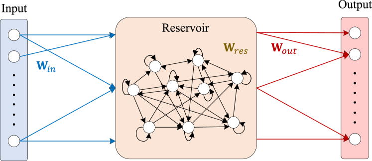
Next, we define the input, output and the model weights of the ESN in the following:

• $\mathbf{x}_{\mathrm{res}}[n]\in\mathbb{R}^{M}$ is the state vector at the time index $n$.

• $\mathbf{X}_{\mathrm{res}}=\big{[}\mathbf{x}_{\mathrm{res}}[1],\cdots,\mathbf{x}_{\mathrm{res}}[T]\big{]}\in\mathbb{R}^{M\times T}$ is defined as the “reservoir states matrix” of the individual states across time from $n=1$ to the end of the input sequence $n=T$ stacked sequentially.

• $\mathbf{x}_{\mathrm{in}}[n]\in\mathrm{R}^{D}$ denotes the ESN input. $\mathbf{y}[n]\in\mathbb{R}^{K}$ denotes the ESN output.

• $\mathbf{W}_{\mathrm{in}}\in\mathbb{R}^{M\times D}$ is the input weights matrix, $\mathbf{W}_{\mathrm{res}}\in\mathbb{R}^{M\times M}$ is the reservoir weights matrix, $\mathbf{W}_{\mathrm{out}}\in\mathbb{R}^{K\times M}$ is the output weights matrix.

If $\sigma(\cdot)$ is a pointwise non-linear activation function, the state update equation and the output equation are respectively:

$$\mathbf{x}_{\text{res}}[n] =\sigma\big{(}\mathbf{W}_{\text{res}}\mathbf{x}_{\text{res}}[n-1]+\mathbf{W}_{\text{in}}\mathbf{x}_{\text{in}}[n]\big{)},$$ (1)

$$\mathbf{y}[n] =\mathbf{W}_{\text{out}}\mathbf{x}_{\text{res}}[n].$$ (2)

In this setup, $\mathbf{W}_{\text{in}}$ and $\mathbf{W}_{\text{res}}$ are initialized from a certain pre-determined distribution, e.g., the uniform or Gaussian (Normal) distributions, and then kept fixed throughout the training and inference (test) stages. Unlike vanilla RNNs and its variants where all network weights are trained using BPTT, the only trainable network parameter in the ESN is $\mathbf{W}_{\text{out}}$, which is trained using a pseudoinverse-based closed-form linear update rule. This greatly reduces the number of trainable parameters as well as the training computational complexity, lending well to applications with limited training data availability. Additionally, the sparsity of $\mathbf{W}_{\text{res}}$ is controlled via the hyperparameter named ‘sparsity’ (denoted as $\kappa$), which represents the probability of an element of $\mathbf{W}_{\text{res}}$ being zero. The internal reservoir structure of Fig. 1 depicts this random and potentially sparse nature of the interconnections between the constituent neurons.

II-B Simulating a basic LTI System with an ESN

Consider the target system as characterized by the following time-domain impulse response

$$\mathbf{s}_{\alpha}[n]= \begin{cases}\alpha^{n},&n\geq 0\\ 0,&n<0\end{cases}=\alpha^{n}u[n],$$ (3)

where $\alpha\in\mathbb{R}$, $\alpha<1$ and $u[n]$ is the discrete-time unit step function. Thus, the target system to be simulated or estimated by the ESN is described by the time-domain impulse response characterized by the infinite-dimensional vector $\mathbf{s}_{\alpha}\in\mathbb{R}^{\infty}$. We choose this as the first case to analyze since the time-domain impulse response of a general LTI system can be written as a linear combination of the impulse response of Eq. (3), i.e.,

$$\mathbf{h}[n]=\sum_{i=1}^{N_{0}}w_{i}\mathbf{s}_{\alpha_{i}}[n],$$ (4)

where $w_{i}\in\mathbb{R}$ are the combining weights, thereby making the extension to the general case feasible given the analysis for the simple case of Eq. (3).

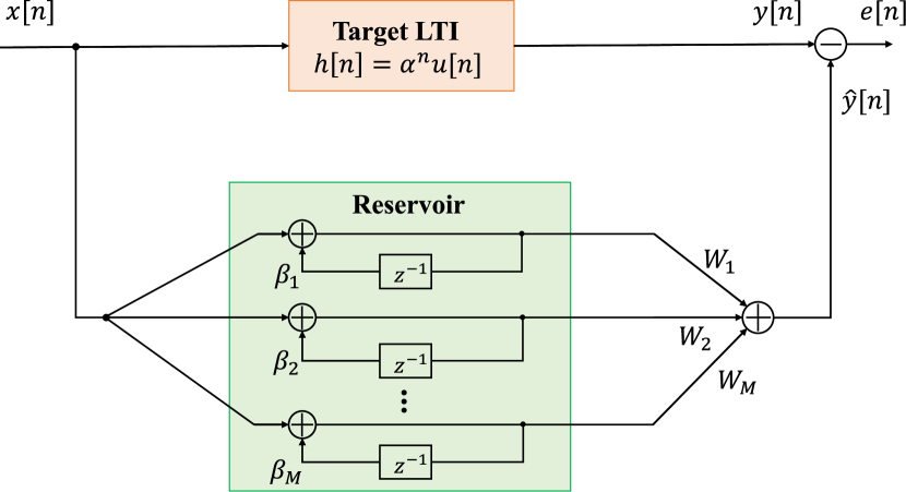
In this work, we consider a simplified version of the more general ESN described in Sec. II-A. Specifically, we consider a simple reservoir construction where the individual neurons are disconnected from each other and only consist of unit delay self-feedback loops. This translates to $\mathbf{W}_{\mathrm{res}}$ being a diagonal matrix. Secondly, for tractability of analysis, we consider linear activation such that $\sigma(\cdot)$ in Eq. (1) is an identity mapping. As shown in our previous work [44], a single neuron with linear activation can be modeled as a first-order infinite impulse response (IIR) filter with a single pole. This is illustrated in Fig. 2, where a single neuron or “node” inside the reservoir simply implements a first-order autoregressive process AR(1) with a feedback weight $a$. The system response for the IIR filter in Fig. 2 is given by

$$H_{0}(z)=\frac{X_{\mathrm{out}}(z)}{X_{\mathrm{in}}(z)}=\frac{1}{1-az^{-1}}.$$ (5)

Finally, we consider the input weights to be unity, as their effect is absorbed in the output weights when the activation employed in the reservoir is linear.

Figure 2: Modeling a neuron in the reservoir with linear activation as a single-pole IIR filter.

With the aforementioned preliminaries laid out, the ESN design problem for LTI system simulation can be articulated as follows. Consider an ESN reservoir as a collection of neurons with corresponding reservoir (recurrent) weights $\{\beta_{1},\beta_{2},\ldots,\beta_{M}\}$, where each $\beta_{m}\in\mathbb{R}$. We would like to choose $\{\beta_{1},\ldots,\beta_{M}\}$ such that their weighted combination approximates the normalized target $\frac{\mathbf{s}_{\alpha}}{\|\mathbf{s}_{\alpha}\|_{2}}$ with a low approximation error, i.e.,

$$\frac{\mathbf{s}_{\alpha}}{\|\mathbf{s}_{\alpha}\|_{2}}\approx\sum_{m=1}^{M}W_{m}\mathbf{s}_{\beta_{m}},$$ (6)

where $\mathbf{s}_{\beta_{m}}[n]=\beta_{m}u[n]$. Note that target normalization is imperative to ensure that the mean approximation error across multiple realizations $\alpha$ of the random variable $\mathrm{A}$ is not dominated by realizations for which $\alpha$ is closer to $1$ or $-1$ over those for which $\alpha$ is closer to $0$. With this formulation, the normalized target has unit norm. This can also be written as the system function in terms of the $z$-transform as

$$S_{\alpha}(z)\approx\sum_{m=1}^{M}W_{m}S_{\beta_{m}}(z),$$ (7)

which can be expanded as

$$\frac{\sqrt{1-\alpha^{2}}}{1-\alpha z^{-1}}\approx\sum_{m=1}^{M}\frac{W_{m}}{1-\beta_{m}z^{-1}}.$$ (8)

Thus, the system being estimated is an infinite impulse response (IIR) system with a single pole $\alpha$, while the ESN attempts to estimate this IIR system with a weighted combination of $M$ IIR systems, each characterized by a pole $\beta_{m}$. This problem can also be characterized as a system “simulation” problem, whereby a linear ESN with a reservoir of non-interconnected neurons attempts to reproduce the output of the unknown LTI system belonging to a known model family, in this case, a single-pole IIR system. This “system simulation” problem is visually depicted in Fig. 3.

Figure 3: Simulating an LTI system belonging to a known model family (e.g., first-order IIR system) with a linear non-interconnected reservoir ESN.

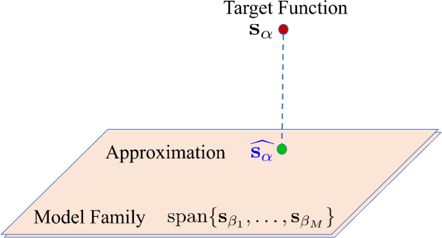
Eq. (6) can be viewed as a projection problem where the best-case approximation of $\mathbf{s}_{\alpha}$ with $\{\mathbf{s}_{\beta_{m}}\}_{m=1}^{M}$ is obtained when $\mathbf{s}_{\alpha}$ is orthogonally projected onto the linear subspace $\operatorname{span}(\mathbf{s}_{\beta_{1}},\ldots,\mathbf{s}_{\beta_{M}})$. This is illustrated in Fig. 4.

Figure 4: Learning a single-pole IIR system viewed as an orthogonal projection problem.

Therefore, the corresponding projection error can be written as the $\ell_{2}$-loss given by

$$\varepsilon=\left\|\frac{\mathbf{s}_{\alpha}}{\|\mathbf{s}_{\alpha}\|_{2}}-\sum_{m=1}^{M}W_{m}^{*}\mathbf{s}_{\beta_{m}}\right\|_{2}^{2},$$ (9)

where

$$\{W_{m}^{*}\}=\operatorname*{arg\,min}_{\{W_{m}\}}\left\|\frac{\mathbf{s}_{\alpha}}{\|\mathbf{s}_{\alpha}\|_{2}}-\sum_{m=1}^{M}W_{m}\mathbf{s}_{\beta_{m}}\right\|_{2}^{2}.$$ (10)

Then, the optimum output weights are given by

$$\mathbf{w}=\mathbf{\Sigma}^{-1}\mathbf{r},$$ (11)

where $\mathbf{w}\overset{\mathrel{\raisebox{-0.43057pt}{\scalebox{0.8}[0.6]{$\vartriangle$}}}}{=}[W_{1}^{*}\;\ldots\;W_{M}^{*}]^{T}\in\mathbb{R}^{M}$, and the projection error can be shown to be

$$\varepsilon=1-\mathbf{r}^{T}\mathbf{\Sigma}^{-1}\mathbf{r}.$$ (12)

Here, $\|\mathbf{s}_{\alpha}\|_{2}^{2}=\sum_{n=0}^{\infty}\alpha^{2n}=\frac{1}{1-\alpha^{2}}$, and $\mathbf{r}\in\mathbb{R}^{M\times 1}$ and $\mathbf{\Sigma}\in\mathbb{R}^{M\times M}$ are respectively defined as

$$\mathbf{r}\overset{\mathrel{\raisebox{-0.43057pt}{\scalebox{0.8}[0.6]{$\vartriangle$}}}}{=}\frac{1}{\|\mathbf{s}_{\alpha}\|_{2}}\begin{bmatrix}\langle\mathbf{s}_{\beta_{1}},\mathbf{s}_{\alpha}\rangle\\ \vdots\\ \langle\mathbf{s}_{\beta_{M}},\mathbf{s}_{\alpha}\rangle\end{bmatrix},$$ (13)

and $[\mathbf{\Sigma}]_{i,j}\overset{\mathrel{\raisebox{-0.43057pt}{\scalebox{0.8}[0.6]{$\vartriangle$}}}}{=}\langle\mathbf{s}_{\beta_{i}},\mathbf{s}_{\beta_{j}}\rangle$, where $[\mathbf{\Sigma}]_{i,j}$ is the element of $\mathbf{\Sigma}$ in the $i^{\text{th}}$ row and the $j^{\text{th}}$ column.

Stated in machine learning terms, the projection error of Eq. (12) can be viewed as a lower bound on both the training loss as well as the test loss. Additionally, it is inherently assumed that an infinite number of samples are available for training such that the weights $\{W_{m}\}$ are set to to their optimum values $\{W_{m}^{*}\}$. Thus, the error of Eq. (12) is the lowest achievable training loss and we can define the training loss $\mathcal{L}(\cdot;\cdot)$ (trained on infinitely many samples) to be the projection error of Eq. (9), i.e.,

$$\mathcal{L}(\alpha;\beta_{1},\ldots,\beta_{M})\overset{\mathrel{\raisebox{-0.43057pt}{\scalebox{0.8}[0.6]{$\vartriangle$}}}}{=}\varepsilon.$$ (14)

The ultimate ESN design goal is to analytically choose the optimal $\{\beta_{1}^{*},\ldots,\beta_{M}^{*}\}$ such that

$$\{\beta_{1}^{*},\ldots,\beta_{M}^{*}\}=\operatorname*{arg\,min}_{\{\beta_{1},\ldots,\beta_{M}\}}\mathbb{E}_{\alpha\sim p_{\mathrm{A}}(\alpha)}\big{[}\mathcal{L}(\alpha;\beta_{1},\ldots,\beta_{M})\big{]},$$ (15)

so that the expected training loss is minimized, where the expectation is taken over multiple realizations of the target function parameter $\alpha$, for which a prior probability distribution $p_{\mathrm{A}}(\alpha)$ is known. Stated explicitly, we model the pole of the first-order IIR system as a random variable $\mathrm{A}$ with a particular realization or observed value denoted as $\alpha$.

Determining the optimum $\{\beta_{m}^{*}\}_{m=1}^{M}$ individually can be intractably challenging. Hence, we take an alternate approach. Instead of finding the optimum reservoir weights individually, we attempt to find the optimal probability distribution $p_{\mathrm{B}}^{*}(\beta)$, from which the poles $\{\beta_{1},\ldots,\beta_{M}\}$ are drawn in an i.i.d. fashion. Therefore, the reservoir optimization problem can be reformulated as determining the optimal ESN pole distribution $p_{\mathrm{B}}^{*}(\beta)$ where

$$p_{\mathrm{B}}^{*}(\beta)$$

$$=\operatorname*{arg\,min}_{p_{\mathrm{B}}(\beta)}\mathbb{E}_{\{\beta_{1},\ldots,\beta_{M}\}\overset{\text{i.i.d.}}{\sim}p_{\mathrm{B}}(\beta)}\bigg{[}\mathbb{E}_{\alpha\sim p_{\mathrm{A}}(\alpha)}\big{[}\mathcal{L}(\alpha;\beta_{1},\ldots,\beta_{M})\big{]}\bigg{]}.$$ (16)

In the next section, we describe a method of solving this optimization problem by using a local approximation.

Figure 5: Projection Error ($\varepsilon$) of Eq. (12) versus $\alpha$ for $M=5,7,9$ ESN poles evenly spaced in $(-1,1)$. The local minima represent the locations of the poles $\{\beta_{m}\}_{m=1}^{M}$ in each case.

III Reservoir Optimization

III-A Nearest Neighbors Approximation

As $M\rightarrow\infty$, the true training loss $\mathcal{L}(\alpha;\beta_{1},\ldots,\beta_{M})$ can be estimated by making a “nearest neighbors approximation”, i.e., in the neighborhood of a given $\alpha$, the approximation error due to $\{\beta_{m}\}_{m=1}^{M}$ is dominated by the two ESN poles closest to $\alpha$. In this treatment, we assume that $\alpha\sim\mathcal{U}(-\alpha_{0},\alpha_{0})\overset{\mathrel{\raisebox{-0.43057pt}{\scalebox{0.8}[0.6]{$\vartriangle$}}}}{=}p_{\mathrm{A}}(\alpha;\alpha_{0})$, where $0<\alpha_{0}<1$. Then, the nearest neighbor approximation states that

$$\mathcal{L}(\alpha;\beta_{1},\ldots,\beta_{M})\approx\widetilde{\mathcal{L}}(\alpha;\beta_{1},\ldots,\beta_{M}),$$ (17)

where the “surrogate loss” $\widetilde{\mathcal{L}}$ is defined as

$$\widetilde{\mathcal{L}}(\alpha;\beta_{1},\ldots,\beta_{M})\overset{\mathrel{\raisebox{-0.43057pt}{\scalebox{0.8}[0.6]{$\vartriangle$}}}}{=}\mathcal{L}(\alpha;\beta^{(1)},\beta^{(2)}).$$ (18)

Here, $\beta^{(1)}$ and $\beta^{(2)}$ are the two ESN poles that are closest to $\alpha\in\mathcal{R}$, i.e., its two nearest neighbors in the small neighborhood $\mathcal{R}$ within $[-\alpha_{0},\alpha_{0}]$, with $\beta^{(1)},\beta^{(2)}\subset\{\beta_{1},\ldots,\beta_{M}\}$. These “neighborhood losses” can be calculated for each value of $\alpha$ as it is swept inside the region $(-\alpha_{0},\alpha_{0})$. With the approximation of Eq. (17), the optimization problem can be stated as

$$p_{\mathrm{B}}^{*}(\beta)$$

$$=\operatorname*{arg\,min}_{p_{\mathrm{B}}(\beta)}\mathbb{E}_{\{\beta_{m}\}_{m=1}^{M}\overset{\text{i.i.d.}}{\sim}p_{\mathrm{B}}(\beta)}\Bigg{[}\mathbb{E}_{\alpha\sim p_{\mathrm{A}}(\alpha;\alpha_{0})}\bigg{[}\widetilde{\mathcal{L}}\left(\alpha;\{\beta_{m}\}_{m=1}^{M}\right)\bigg{]}\Bigg{]}.$$ (19)

If the training loss corresponding to the problem in Eq. (19) is $\varepsilon_{1}$, i.e.,

$$\varepsilon_{1}$$

$$=\min_{p_{\beta}}\mathbb{E}_{\{\beta_{1},\ldots,\beta_{M}\}\overset{\text{i.i.d.}}{\sim}p_{\mathrm{B}}(\beta)}\bigg{[}\mathbb{E}_{\alpha\sim p_{\mathrm{A}}(\alpha;\alpha_{0})}\big{[}\widetilde{\mathcal{L}}(\alpha;\beta_{1},\ldots,\beta_{M})\big{]}\bigg{]},$$

$$=\min_{p_{\beta}}\mathbb{E}_{\{\beta_{1},\ldots,\beta_{M}\}\overset{\text{i.i.d.}}{\sim}p_{\beta}}\bigg{[}\sum_{\mathcal{R}}\int_{\alpha\in\mathcal{R}}p_{\mathrm{A}}(\alpha)\widetilde{\mathcal{L}}(\alpha;\beta_{1},\ldots,\beta_{M})d\alpha\bigg{]},$$

$$=\min_{p_{\beta}}\mathbb{E}_{\{\beta_{1},\ldots,\beta_{M}\}\overset{\text{i.i.d.}}{\sim}p_{\beta}}\bigg{[}\sum_{\mathcal{R}}\int_{\alpha\in\mathcal{R}}p_{\mathrm{A}}(\alpha)\mathcal{L}\left(\alpha;\beta^{(1)},\beta^{(2)}\right)d\alpha\bigg{]},$$

$$=\min_{p_{\beta}}\mathbb{E}_{\{\beta_{1},\ldots,\beta_{M}\}\overset{\text{i.i.d.}}{\sim}p_{\beta}}\bigg{[}\sum_{\mathcal{R}}\Pr(\alpha\in\mathcal{R})\cdot\mathcal{L}\left(\alpha;\beta^{(1)},\beta^{(2)}\right)\bigg{]},$$ (20)

then clearly $\varepsilon_{1}\leq\varepsilon_{2}$, where

$$\varepsilon_{2}=\min_{p_{\beta}}\mathbb{E}_{\{\beta_{m}\}\overset{\text{i.i.d.}}{\sim}p_{\beta}}\bigg{[}\sum_{\mathcal{R}}\Pr(\alpha\in\mathcal{R})\sup_{\alpha\in\mathcal{R}}\big{[}\mathcal{L}(\alpha;\beta^{(1)},\beta^{(2)})\big{]}\bigg{]}.$$ (21)

Since $\Pr(\alpha\in\mathcal{R})$ is the same regardless of the location of the small neighborhood $\mathcal{R}$ in the entire range of $[-\alpha_{0},\alpha_{0}]$ for uniformly distributed $\mathrm{A}$, the optimization problem can be stated as the min-max formulation given by

$$p_{\beta}^{*}=\operatorname*{arg\,min}_{p_{\beta}}\mathbb{E}_{\{\beta_{1},\ldots,\beta_{M}\}\overset{\text{i.i.d.}}{\sim}p_{\beta}}\bigg{[}\sum_{\mathcal{R}}\sup_{\alpha\in\mathcal{R}}\big{[}\mathcal{L}(\alpha;\beta^{(1)},\beta^{(2)})\big{]}\bigg{]}.$$ (22)

Therefore, we would like to balance the supremum of the error within the small neighborhood $\mathcal{R}$ across all such neighborhoods $\mathcal{R}$ in $(-\alpha_{0},\alpha_{0})$. At this point, it is instructive to analyze the behavior of the error $\mathcal{L}\left(\alpha;\beta^{(1)},\beta^{(2)}\right)$ in the small neighborhood $\mathcal{R}$. Specifically, we analyze the projection error $\varepsilon$ with $M=2$ in Eq. (12). This is investigated next.

III-B Optimization with Nearest Neighbor Approximation

We analyze the behavior of the error of Eq. (12) in the small neighborhood $\mathcal{R}$ where the two nearest neighbors of $\alpha\in\mathcal{R}$, $\beta^{(1)}$ and $\beta^{(2)}$ are denoted simply as $\beta_{1}$ and $\beta_{2}$ for clarity of notation, even though the overall actual poles of the ESN have been denoted previously as $\{\beta_{1},\beta_{2},\ldots,\beta_{M}\}$ with $M$ being very large in this nearest neighbors approximation. With this disclaimer, in the following analysis, we denote the projection error of Eq. (12) as $\varepsilon_{(2)}$, where the subscript $(2)$ denotes the fact that we are evaluating a $2$-nearest neighbors error in a small neighborhood $\mathcal{R}$. After substituting for $\mathbf{r}$ and $\mathbf{\Sigma}$ with $M=2$ in Eq. (12) and with further manipulation, $\varepsilon_{(2)}$ can be obtained as

$$\varepsilon_{(2)} =1-\frac{(1-\alpha^{2})(1-\beta_{1}\beta_{2})}{(\beta_{1}-\beta_{2})^{2}}\Bigg{(}\frac{(1-\beta_{1}^{2})(1-\beta_{1}\beta_{2})}{(1-\alpha\beta_{1})^{2}}$$

$$-2\frac{(1-\beta_{1}^{2})(1-\beta_{2}^{2})}{(1-\alpha\beta_{1})(1-\alpha\beta_{2})}+\frac{(1-\beta_{2}^{2})(1-\beta_{1}\beta_{2})}{(1-\alpha\beta_{2})^{2}}\Bigg{)}.$$ (23)

Since our focus is on the small neighborhood $\mathcal{R}$, we quantify the density of packing of the two ESN poles $\beta_{1}$ and $\beta_{2}$ by defining them around a mid-point $\beta$ as $\beta_{1}=\beta-\Delta$ and $\beta_{2}=\beta+\Delta$. Thus, with the width of the small neighborhood $\mathcal{R}$ being $2\Delta$, the average spacing of ESN poles in the entire region $(-\alpha_{0},\alpha_{0})$ is represented by $\Delta$.

We are interested in the trend followed by the maximum value of this error within $\mathcal{R}$ as a function of $\Delta$. However, obtaining an expression for the true maximum error $\varepsilon_{(2)}^{(\mathrm{max})}$ by finding the stationary point inside $\mathcal{R}$ is intractably tedious. Therefore, instead of finding $\varepsilon_{(2)}^{(\mathrm{max})}$, we attempt to find an upper bound $B_{\varepsilon}$ on $\varepsilon_{(2)}^{(\mathrm{max})}$. Our goal is to determine a relationship between $B_{\varepsilon}$ and the average spacing between the poles, characterized by $\Delta$. With this final goal, we state the following proposition.

Proposition 1.

An upper bound on the maximum error in $\mathcal{R}$ is given by

$$B_{\varepsilon}=\varepsilon_{(2)}^{\mathrm{(mid)}}+\Delta\left|\frac{\partial\varepsilon_{(2)}}{\partial\alpha}\bigg{\rvert}_{\alpha=\frac{1}{2}(\beta_{1}+\beta_{2})}\right|,$$ (24)

where $\varepsilon_{(2)}^{\mathrm{(mid)}}\overset{\mathrel{\raisebox{-0.43057pt}{\scalebox{0.8}[0.6]{$\vartriangle$}}}}{=}\varepsilon_{(2)}(\beta)$.

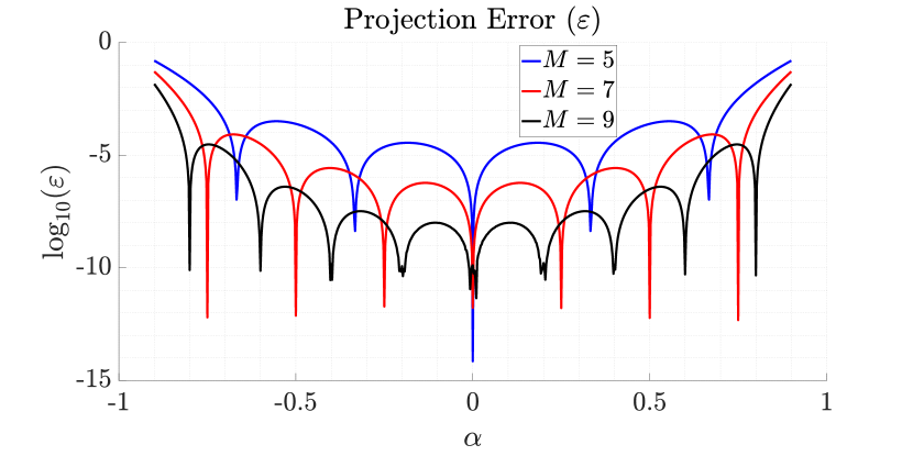
The above can be seen with the help of Fig. 6 which plots the projection error $\varepsilon_{(2)}$ with the nearest neighbors approximation introduced previously. It can be observed that $B_{\varepsilon}$ is one of the possible upper bounds on the true maximum error $\varepsilon_{(2)}\rvert_{\alpha=\alpha_{(\mathrm{max}})}$. Since $\varepsilon_{(2)}$ is a concave function and has exactly one local maximum in the small neighborhood $\mathcal{R}$, the claim of Proposition 1 always holds within $\mathcal{R}$, bounded by exactly one ESN pole on either side.

Figure 6: Projection error $\varepsilon_{(2)}$ plotted in the neighborhood $\mathcal{R}$ with poles $\beta_{1}$ and $\beta_{2}$ on its edges.

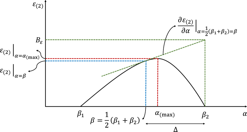
The neighborhood projection error $\varepsilon_{(2)}$ evaluated at the mid-point of $\mathcal{R}$ is expressed in the following lemma.

Lemma 1.

The $2$-nearest neighbors-based projection error $\varepsilon_{(2)}$, evaluated at the mid-point $\alpha=\frac{1}{2}(\beta_{1}+\beta_{2})=\beta$ within the small neighborhood $\mathcal{R}$ is given by

$$\varepsilon_{(2)}^{(\mathrm{mid})}=\frac{1}{(1-\beta^{2})^{4}}\Delta^{4}+O(\Delta^{6}).$$ (25)

The complete proof for this result is provided in Appendix A. This is an important outcome, indicating that the error has a power law scaling with $\Delta$ given by $\Delta^{4}$. Similarly, an expression for $\frac{\partial\varepsilon_{(2)}}{\partial\alpha}\rvert_{\alpha=\beta}$ is given in the following lemma.

Lemma 2.

The rate of change of $\varepsilon_{(2)}$ in $\mathcal{R}$, evaluated at the mid-point $\alpha=\beta$ is given by

$$\frac{\partial\varepsilon_{(2)}}{\partial\alpha}\bigg{\rvert}_{\alpha=\frac{1}{2}(\beta_{1}+\beta_{2})=\beta}=\frac{4\beta}{(1-\beta^{2})^{5}}\Delta^{4}+O(\Delta^{6}).$$ (26)

The complete derivation for this result is given in Appendix B. With these expressions derived and using Eq. (24) of Proposition 1, we can state the following theorem.

Theorem 1.

The upper bound on the worst-case (highest) projection error in $\mathcal{R}$ is governed by the scaling law given by

$$B_{\varepsilon}=\frac{1}{(1-\beta^{2})^{4}}\Delta^{4}+\frac{4|\beta|}{(1-\beta^{2})^{5}}\Delta^{5}+O(\Delta^{6}).$$ (27)

This bound follows directly from substituting Eq. (25) and Eq. (26) in Eq. (24) of Proposition 1. Note that a tighter bound on the true maximum error $\varepsilon_{(2)}^{(\mathrm{max})}$ can be obtained by evaluating the RHS of Eq. (24) at an $\alpha=\alpha^{*}$ that is closer to the true maximizing point $\alpha_{(\mathrm{max})}$ compared to the mid-point $\alpha=\beta$. However, it can be shown that such a tighter bound also exhibits a minimum dependence of $\Delta^{4}$. With either upper bound, the conclusion is that the worst-case projection error in $\mathcal{R}$ obeys a $\Delta$-power scaling law with the minimum exponent $4$ and no lower than that, i.e., the error scales as at least $\Delta^{4}$, which is a significant definitive result. Recognizing that $\Delta\,\propto\,\frac{1}{M}$, where $M$ is the number of neurons in the reservoir, Theorem 1 provides us with a practical scaling law for the ESN training loss, i.e., $\varepsilon_{(2)}^{(\mathrm{max})}\>\propto\>\frac{1}{M^{4}}$. This is a strong statement which directly relates the extent to which the training loss can be lowered by increasing the number of reservoir neurons $M$. Such a direct scaling relationship is currently missing for more traditional neural network architectures.

With an expression for an upper bound on the worst-case projection error derived as in Theorem 1, the optimization problem of Eq. (22) now translates to ensuring the leading term in the upper bound expression stays the same across all neighborhoods $\mathcal{R}$ in $(-\alpha_{0},\alpha_{0})$, i.e., across $\beta\in(-\alpha_{0},\alpha_{0})$. This implies that for a given mid-point $\beta$ of two ESN poles, the spacing $\Delta(\beta)$ must be chosen according to

$$[\Delta(\beta)]^{4}\; \propto\;(1-\beta^{2})^{4},$$

$$\Rightarrow\Delta(\beta)\; \propto(1-\beta^{2}).$$ (28)

Therefore, it follows that the optimal distribution $p_{\mathrm{B}}^{*}(\beta)$ from which the ESN poles $\{\beta_{m}\}_{m=1}^{M}$ are drawn i.i.d. is subject to $p_{\mathrm{B}}^{*}(\beta)\,\propto\,\frac{1}{\Delta(\beta)}$ and thus, can be written as

$$p_{\mathrm{B}}^{*}(\beta)=\frac{1}{C}\frac{1}{(1-\beta^{2})},$$ (29)

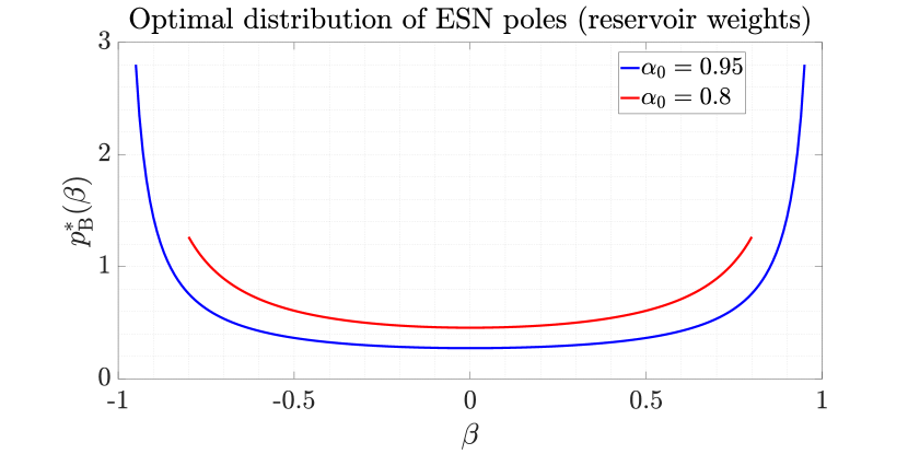
where the normalization constant $C$ is found by solving $\int_{-\alpha_{0}}^{\alpha_{0}}\frac{C}{1-\beta^{2}}d\beta=1$, giving $C=\log(\frac{1+\alpha_{0}}{1-\alpha_{0}})$. As an example for $\alpha=0.95$, $C=3.6636$ and the optimal ESN pole (reservoir weight) distribution $p_{\mathrm{B}}^{*}(\beta)$ is

$$p_{\mathrm{B}}^{*}(\beta)=\frac{0.273}{1-\beta^{2}}.$$ (30)

The optimal probability density function curves for $\alpha_{0}=0.95$ and $\alpha_{0}=0.8$ are plotted in Fig. 7.

Figure 7: Optimal probability density function (PDF) $p_{\mathrm{B}}^{*}(\beta)$ curves shown for $\alpha_{0}=0.95$ and $\alpha_{0}=0.8$.

III-C Incorporating Prior Distributions on pole of LTI system

In our derivation of the optimal ESN pole distribution $p_{\mathrm{B}}^{*}(\beta)$ stated in Eq. (29), the prior on the pole of the unknown LTI system was assumed to be uniformly distributed, i.e., $\mathrm{A}\sim\mathcal{U}(-\alpha_{0},\alpha_{0})$. However, the derived optimal distribution of the poles $\{\beta_{m}\}$ can be adjusted for any other prior distribution given on $\mathrm{A}$. This result is stated in the following corollary.

Corollary 1.1.

Given an optimal probability distribution function $p_{\mathrm{B}}^{*}(\beta)$ of the ESN poles $\{\beta_{m}\}$ for the unknown system pole $\mathrm{A}$ distributed as $\mathrm{A}\sim p_{\mathrm{A}}(\alpha)=\mathcal{U}(-\alpha_{0},\alpha_{0})$, the optimal distribution changes to $q_{\mathrm{B}}^{*}(\beta)\;\propto\;p_{\mathrm{B}}^{*}(\beta)\cdot q_{\mathrm{A}}(\beta)$ if the prior distribution on $\mathrm{A}$ changes to $q_{\mathrm{A}}(\alpha)$.

We proceed to derive the above result via the following sketch of a proof. First, the optimum spacing $\Delta$ between the poles from Eq. (III-B), which is derived for an infinitesimally small neighborhood $\mathcal{R}$, is more accurately written as $\Delta(\mathcal{R})$ and $\beta(\mathcal{R})$. Reverting to the original objective function of Eq. (16) for the projection error to be minimized, we have

$$\min_{p_{\mathrm{B}}(\beta)}\mathbb{E}_{\{\beta_{m}\}\overset{\text{i.i.d.}}{\sim}p_{\mathrm{B}}(\beta)}\bigg{[}\mathbb{E}_{\alpha\sim p_{\mathrm{A}}(\alpha)}\big{[}\mathcal{L}(\alpha;\beta_{1},\ldots,\beta_{M})\big{]}\bigg{]}$$

$$\overset{(a)}{\approx}\min_{p_{\mathrm{B}}(\beta)}\mathbb{E}_{\{\beta_{m}\}}\bigg{[}\sum_{\mathcal{R}}\big{(}p_{\mathrm{A}}(\alpha;\mathcal{R})\cdot\delta\big{)}\frac{1}{(1-\beta(\mathcal{R})^{2})^{4}}[\Delta(\mathcal{R})]^{4}\bigg{]},$$ (31)

where $(a)$ follows from the nearest neighbors approximation and the result of Theorem 1, and $p_{\mathrm{A}}(\alpha;\mathcal{R})\cdot\delta=\Pr(\alpha\in\mathcal{R})$ for a neighborhood $\mathcal{R}$ of width $\delta$. The summation is over a collection of neighborhoods that form a cover of $(-\alpha_{0},\alpha_{0})$. For convenience, we assume that these neighborhoods have equal width $\delta$. $\beta(\mathcal{R})$ and $\Delta(\mathcal{R})$ denote an ESN pole $\beta$ in $\mathcal{R}$ and the spacing between the poles in $\mathcal{R}$ respectively.

Now, it is clear that when designing the optimal pole distribution $p_{\mathrm{B}}^{*}(\beta)$, we would like the summand in Eq. (31) to be balanced in each neighborhood. Specifically, since $p_{\mathrm{A}}(\alpha;\mathcal{R})=p_{\mathrm{A}}(\alpha;\mathcal{R^{\prime}})$ for uniformly distributed $\mathrm{A}$ in any two neighborhoods $\mathcal{R}$ and $\mathcal{R}^{\prime}$, optimality requires

$$\frac{1}{(1-\beta(\mathcal{R})^{2})^{4}}[\Delta(\mathcal{R})]^{4} =\frac{1}{(1-\beta(\mathcal{R}^{\prime})^{2})^{4}}[\Delta(\mathcal{R}^{\prime})]^{4},$$

$$\Rightarrow\frac{1}{1-\beta(\mathcal{R})^{2}}\Delta(\mathcal{R}) =\frac{1}{1-\beta(\mathcal{R}^{\prime})^{2}}\Delta(\mathcal{R}^{\prime}).$$ (32)

Recognizing that $p_{\mathrm{B}}(\mathcal{R})\,\propto\,\frac{1}{\Delta(\mathcal{R})}$, it follows that $p_{\mathrm{B}}^{*}(\mathcal{R})\,\propto\,(1-\beta(\mathcal{R}))^{-1}$. However, when the prior distribution $q_{\mathrm{A}}(\alpha)$ is non-uniform so that $\Pr(\alpha\in\mathcal{R})\neq\Pr(\alpha\in\mathcal{R^{\prime}})$, optimality requires

$$\frac{q_{\mathrm{A}}(\mathcal{R})}{1-\beta(\mathcal{R})^{2}}\Delta(\mathcal{R})=\frac{q_{\mathrm{A}}(\mathcal{R^{\prime}})}{1-\beta(\mathcal{R}^{\prime})^{2}}\Delta(\mathcal{R}^{\prime}).$$ (33)

Since the modified distribution of the poles $q_{\mathrm{B}}(\mathcal{R})$ in $\mathcal{R}$ also follows $q_{\mathrm{B}}(\mathcal{R})\,\propto\,\frac{1}{\Delta(\mathcal{R})}$, the optimal modified pole distribution $q_{\mathrm{B}}^{*}(\mathcal{R})$ satisfies

$$q_{\mathrm{B}}^{*}(\mathcal{R})\,\propto\,\frac{q_{\mathrm{A}}(\mathcal{R})}{1-\beta(\mathcal{R})^{2}}.$$ (34)

Dropping the dependence on the local neighborhood $\mathcal{R}$,

$$q_{\mathrm{B}}^{*}(\beta)\,\propto\,\frac{q_{\mathrm{A}}(\beta)}{1-\beta^{2}}=p_{\mathrm{B}}^{*}(\beta)\cdot q_{\mathrm{A}}(\beta),$$ (35)

giving the result in Corollary 1.1.

III-D Reservoir with Random and Sparse Interconnections

The conventional ESN uses a reservoir that is sparsely connected with random (and randomly weighted) interconnections between the constituent neurons. In the case of non-interconnected neurons in the reservoir, the reservoir weights matrix is $\mathbf{W}_{\mathrm{res}}=\operatorname{diag}\left(\{\beta_{m}\}_{m=1}^{M}\right)$. However, this is not the case for a random and sparsely interconnected reservoir. Performing the eigenvalue decomposition of $\mathbf{W}_{\text{res}}$, we get

$$\mathbf{W}_{\text{res}}=\mathbf{Q}\mathbf{\Lambda}\mathbf{Q}^{-1},$$ (36)

where $\mathbf{Q}\in\mathbb{R}^{M\times M}$ is the matrix containing the eigenvectors of $\mathbf{W}_{\text{res}}$. For a non-interconnected reservoir, $\mathbf{W}_{\text{res}}=\mathbf{\Lambda}$ and $\mathbf{Q}=\mathbf{I}_{M}$. On the other hand, for a random and sparsely interconnected reservoir, the elements of $\mathbf{W}_{\text{res}}$ induce a corresponding distribution in $\mathbf{\Lambda}$ such that the elements of $\mathbf{\Lambda}$ may no longer be independent [45]. However, the projection error due to a general random sparsely interconnected reservoir ESN will always be lower bounded by the projection error due to a non-interconnected reservoir with its weights sampled i.i.d. from $p_{\mathrm{B}}^{*}(\beta)$. Although $p_{\mathrm{B}}^{*}(\beta)$ has been derived for the case of non-interconnected neurons, we will show in this section that even with random and sparse (weighted) interconnections between the neurons, where the recurrent and interconnection weights are drawn from a uniform distribution, the projection error in this case is still lower bounded by the projection error with $\{\beta_{m}\}\overset{\text{i.i.d.}}{\sim}p_{\mathrm{B}}^{*}(\beta)$. This can be seen by invoking the state update and output equations for the linear ESN, i.e.,

$$\mathbf{x}_{\text{res}}[n] =\mathbf{W}_{\text{res}}\mathbf{x}_{\text{res}}[n-1]+\mathbf{W}_{\text{in}}\mathbf{x}_{\text{in}}[n]$$ (37)

$$\mathbf{x}_{\text{out}}[n] =\mathbf{W}_{\text{out}}\mathbf{x}_{\text{res}}[n]$$ (38)

Substituting Eq. (36) in Eq. (37), we get

$$\mathbf{x}_{\text{res}}[n] =\mathbf{Q}\mathbf{\Lambda}\mathbf{Q}^{-1}\mathbf{x}_{\text{res}}[n-1]+\mathbf{W}_{\text{in}}\mathbf{x}_{\text{in}}[n],$$

$$\Rightarrow\widetilde{\mathbf{x}}_{\text{res}}[n] =\mathbf{\Lambda}\widetilde{\mathbf{x}}_{\text{res}}[n-1]+\widetilde{\mathbf{W}}_{\text{in}}\mathbf{x}_{\text{in}}[n],$$ (39)

where $\widetilde{\mathbf{x}}_{\text{res}}[n]\overset{\mathrel{\raisebox{-0.43057pt}{\scalebox{0.8}[0.6]{$\vartriangle$}}}}{=}\mathbf{Q}^{-1}\mathbf{x}_{\text{res}}[n]$ and $\widetilde{\mathbf{W}}_{\text{in}}\overset{\mathrel{\raisebox{-0.43057pt}{\scalebox{0.8}[0.6]{$\vartriangle$}}}}{=}\mathbf{Q}^{-1}\mathbf{W}_{\text{in}}$. Using $\mathbf{Q}\mathbf{Q}^{-1}=\mathbf{I}_{M}$ in Eq. (38), we get

$$\mathbf{x}_{\text{out}}[n]=\widetilde{\mathbf{W}}_{\text{out}}\widetilde{\mathbf{x}}_{\text{res}}[n],$$ (40)

where $\widetilde{\mathbf{W}}_{\text{out}}=\mathbf{W}_{\text{out}}\mathbf{Q}$. Thus, a general linear ESN with random and sparse interconnections between its reservoir neurons can be diagonalized and the analysis for its optimization is the same as that for a reservoir without interconnections, i.e., for $\mathbf{W}_{\text{res}}=\mathbf{\Lambda}$. We will empirically show in Sec. V that a reservoir with random interconnections does not provide additional performance gain and is still bounded by the performance of the non-interconnected reservoir ESN with weights sampled from the optimal $p_{\mathrm{B}}^{*}(\beta)$. This conclusion holds in general for reservoirs with linear activation. The effect of nonlinear activation on random interconnections between neurons will be addressed in our future work.

IV Training with Limited Samples

In the preceding sections, we have considered the orthogonal projection of an LTI system’s impulse response on to the subspace spanned by the reservoir of the ESN, and solved the problem of finding the optimum basis for this subspace. Specifically, given a prior distribution of the pole $\alpha$ of a first-order IIR system, we have derived the optimum probability distribution of the reservoir weights for constructing an approximator or system simulator using a linear ESN. The optimum output weights for the linear combination of these basis functions (each characterized by $\beta_{m}$) are given by Eq. (11). Note that this makes use of the knowledge of $\alpha$ or alternatively requires infinitely many samples to learn the optimum output weights $\mathbf{w}$. In practice, however, we do not observe or know the true model of the system being simulated, but rather only have access to a set of limited number of known (or labeled) output samples from the system (known as ground truth) for the corresponding set of input samples. Under this scenario, we train the output weights $\mathbf{w}$ of the ESN with limited training data using the conventional approach. For a training sequence composed of input-output pairs $\{(x_{1},y_{1}),\ldots,(x_{L},y_{L})\}$, the output weights vector is estimated as

$$\widehat{\mathbf{w}}=\left(\boldsymbol{y}^{T}\mathbf{X}_{\text{res}}^{\dagger}\right)^{T},$$ (41)

where $\boldsymbol{y}\overset{\mathrel{\raisebox{-0.43057pt}{\scalebox{0.8}[0.6]{$\vartriangle$}}}}{=}[y_{1}\>y_{2}\,\ldots\>y_{L}]\in\mathbb{R}^{L}$ is the ground truth to be estimated and $\mathbf{X}_{\text{res}}\in\mathbb{R}^{M\times L}$ is the reservoir states matrix containing the state vector from $n=1$ to $n=L$ in its columns. When multiple sequences are used for training, each containing $L$ samples, the training rule becomes

$$\widehat{\mathbf{w}}=\left(\widebar{\boldsymbol{y}}^{T}\widebar{\mathbf{X}}_{\mathrm{res}}^{\dagger}\right)^{T},$$ (42)

where $\widebar{\boldsymbol{y}}\in\mathbb{R}^{N_{p}L}$ is the concatenated ground truth across $N_{p}$ training sequences, and $\widebar{\mathbf{X}}_{\mathrm{res}}\in\mathbb{R}^{M\times N_{p}L}$ is the concatenated reservoir states matrix. The availability of only finite number of labeled training data samples leads to the conundrum of model selection. In the context of reservoir computing and specifically echo state networks, the model selection problem translates to selecting an optimum value for the reservoir size $M$, i.e., the number of poles such that the test loss is minimized without selecting an excessively large reservoir size that may lead to overfitting. Therefore, a penalty term is usually added to the “training loss” to compensate for overfitting and arrive at an appropriate model size. The Akaike Information Criterion (AIC) [46] is a well-known criterion that penalizes large model sizes. The main result of the AIC-based model selection criterion can be written as

$$\operatorname*{arg\,min}_{M}D\left(p_{X,Y}(x,y;\alpha)||p_{X,Y}(x,y;\beta_{m},W_{m})\right)$$

$$=\operatorname*{arg\,min}_{M}D\left(\widehat{p}_{X,Y}(x,y;\alpha)||p_{X,Y}(x,y;\beta_{m},W_{m})\right)+\frac{M}{N_{p}},$$ (43)

where $p_{X,Y}(x,y;\alpha)$ denotes the true unknown joint distribution with parameter $\alpha$ from which the input-output sample pairs are generated, i.e., the unknown LTI system. $p_{X,Y}(x,y;\beta_{m},W_{m})$ denotes the joint distribution generated by the ESN model with parameters $\{\beta_{m}\}$ and $\{W_{m}\}$ and $D(p||q)$ denotes the Kullback-Leibler (KL) divergence between two probability distributions $p(\cdot)$ and $q(\cdot)$. Since we cannot observe the true distribution $p_{X,Y}(x,y;\alpha)$ in practice and are limited to observing only a finite number of input-output samples from the unknown LTI system, we only have access to the empirical distribution $\widehat{p}_{X,Y}(x,y;\alpha)$. With this setup, the argument of the LHS of Eq. (43) is representative of the test loss, while the argument of the first term on the RHS of Eq. (43) is representative of the training loss computed using a finite number $N_{p}$ of input-output pair sequences, for which we have derived a scaling law as a function of $M$ in Theorem 1. The second term on the RHS $\frac{M}{N_{p}}$ represents the penalty imposed by the AIC. Therefore, for the purpose of order analysis of the model selection problem, we can write

$$\mathcal{L}_{\text{test}}\;\propto\;\frac{1}{M^{4}}+\frac{M}{N_{p}}$$ (44)

With this relationship, we can derive an order for the optimum reservoir size $M^{*}$ which minimizes the test loss $\mathcal{L}_{\text{test}}$. This is obtained by first setting

$$\frac{d\mathcal{L}_{\text{test}}}{dM}\;\propto\;-\frac{4}{M^{5}}+\frac{1}{N_{p}}=0$$ (45)

Solving this, we can obtain an order of magnitude for the optimum reservoir size $M^{*}$ as

$$M^{*}=O\left(N_{p}^{1/5}\right).$$ (46)

Note that this result does not give the exact reservoir size in neurons, but rather is an approximation of the order of the optimum reservoir size needed to minimize the testing loss. Furthermore, the AIC is one of many criteria, e.g., Bayesian Information Criterion (BIC), Generalized Information Criterion (GIC) among many others [47] that can be used for model selection in machine learning models spanning simple linear classifiers to deep learning models. This subject is investigated more generally for deep neural networks in the field of statistical learning theory under the umbrella of generalization error analysis. In our previous work [42], we have derived a generalization error bound for ESNs showing lower generalization gap compared to conventional RNNs and developed a model selection framework using the derived bound in the context of ESNs utilized in wireless symbol detection. A similar framework using information theoretic-tools can be developed for model selection in the context of LTI system simulation with an ESN, however that is outside the scope of this paper.

V Numerical Evaluations

In this section, we provide numerical evaluations to validate the theoretical results derived in the preceding sections. Specifically, we aim to experimentally verify the outcome of Theorem 1 and demonstrate the optimality of the distribution $p_{\mathrm{B}}^{*}(\beta)$ for the reservoir weights under various scenarios.

V-A Sampling from the Optimal Distribution

For the case of uniformly distributed system pole $\mathrm{A}$ with realizations $\{\alpha\}$, we use the Von Neumann rejection sampling method (accept-reject algorithm) [48] to draw i.i.d. samples from the optimal reservoir weights distribution $p_{\mathrm{B}}^{*}(\beta)$. Alternatively for a simpler implementation, its empirical form namely, the empirical supremum rejection sampling method [49] can also be used while avoiding computation of the proportionality constant in the PDF for different values of $\alpha_{0}$.

V-B Projection Error Scaling Law from Theorem 1

The main result of Theorem 1 is a scaling law for the projection error as a function of the reservoir size in neurons. This is a key result that also translates to the rate of decrease in the training loss when training a standard linear ESN under limited training data. The projection error of Eq. (12) is simulated over $10^{5}$ Monte-Carlo runs for $\alpha\sim\mathcal{U}(-0.95,0.95)$ and the resulting plot of the empirical projection error ($\varepsilon$) versus $M$ is shown in Fig. 8. We can observe that the simulated projection error using reservoir weights $\{\beta_{m}\}$ drawn from the derived optimal distribution $p_{\mathrm{B}}^{*}(\beta)$ is significantly lower than the error obtained using reservoir weights drawn from $\mathcal{U}(-0.95,0.95)$.

Figure 8: Validation of the scaling law for the projection error ($\varepsilon$) of Eq. (12)

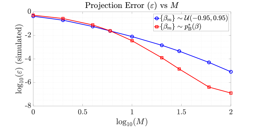
Additionally, it can be empirically observed that $\varepsilon$ approximately displays a $M^{-4}$ dependence on the reservoir size (number of ESN poles) with the weights sampled from the optimal distribution, compared to approximately $M^{-2}$ dependence displayed when the weights are sampled from $\mathcal{U}(-0.95,0.95)$. This indicates a good match between the derived theory and simulation.

In addition to plotting the projection error, we also validate the scaling law via the empirical sequence approximation error $\varepsilon_{\mathrm{seq}}$, defined as

$$\varepsilon_{\mathrm{seq}}=\frac{1}{N_{\mathrm{sim}}L}\sum_{i=1}^{N_{\mathrm{sim}}}\|\mathbf{y}^{(i)}_{\mathrm{LTI}}-\mathbf{y}^{(i)}_{\mathrm{ESN}}\|_{2}^{2},$$ (47)

where $\mathbf{y}^{(i)}_{\mathrm{LTI}}\in\mathbb{R}^{L}$ and $\mathbf{y}^{(i)}_{\mathrm{ESN}}\in\mathbb{R}^{L}$ are the sequences each of length $T$ output by the unknown LTI system being simulated and by the ESN approximation respectively in the $i^{\text{th}}$ Monte-Carlo run. Note that the output weights $\mathbf{w}\in\mathbb{R}^{M}$ for the sequence approximation task are computed using Eq. (11), i.e., they minimize the projection error given the value of the realization $\alpha$ of $\mathrm{A}$ in each run. This simulation result is plotted in Fig. 9 for a sequence length $L=1000$ over $N_{\text{sim}}=10^{5}$ Monte-Carlo runs.

Figure 9: Validation of the scaling law for the sequence approximation error ($\varepsilon_{\mathrm{seq}}$) for sequence length $L=1000$.

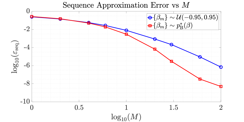
As with the simulated projection error, Fig. 9 shows that the sequence approximation error also exhibits a dependence of approximately $M^{-4}$ for $\{\beta_{m}\}\sim p_{\mathrm{B}}^{*}(\beta)$ and that of approximately $M^{-2}$ for $\{\beta_{m}\}\sim\mathcal{U}(-0.95,0.95)$. In summary, these numerical evaluations provide strong confirmation for the validity of the derived theoretical optimum distribution of the internal reservoir weights.

V-C Error Scaling under Limited Training Data

Although the scaling law for the projection error has been derived under the availability of infinitely many training samples, we can empirically show that a similar trend is also observed in the training loss when the linear ESN is trained with limited data samples, following the standard pseudo-inversion method (with or without regularization) described in Sec. IV. Furthermore, the optimality of the derived distribution $p_{\mathrm{B}}^{*}(\beta)$ is seen in both the empirical training loss as well as the testing loss. The ESN is trained with $N_{p}=1$ training sequence and is tested with $N_{d}=10$ test sequences of length $L=500$ samples. The empirical training loss $\mathcal{L}_{\mathrm{train}}\overset{\mathrel{\raisebox{-0.43057pt}{\scalebox{0.8}[0.6]{$\vartriangle$}}}}{=}\frac{1}{N_{\mathrm{sim}}N_{p}L}\sum_{i=1}^{N_{\mathrm{sim}}}\|\widebar{\mathbf{y}}^{(i)}_{\mathrm{LTI,train}}-\widebar{\mathbf{y}}^{(i)}_{\mathrm{ESN,train}}\|_{2}^{2}$ is plotted in Fig. 10, where $\widebar{\mathbf{y}}^{(i)}_{\mathrm{LTI,train}}\in\mathbb{R}^{N_{p}L}$ is the concatenated training output from the LTI system and $\widebar{\mathbf{y}}^{(i)}_{\mathrm{ESN,train}}\in\mathbb{R}^{N_{p}L}$ is the concatenated ESN output during training respectively in the $i^{\mathrm{th}}$ Monte-Carlo run.

Figure 10: Training loss versus reservoir size $M$ for ESN trained with finite training samples.

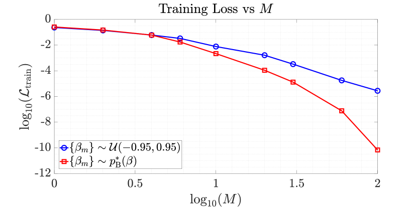
We can observe that the ESN with optimally sampled reservoir weights shows a significantly lower training loss and approximately obeys the $M^{-4}$ scaling law. The more important practical performance metric, namely the empirical test loss $\mathcal{L}_{\mathrm{test}}\overset{\mathrel{\raisebox{-0.43057pt}{\scalebox{0.8}[0.6]{$\vartriangle$}}}}{=}\frac{1}{N_{\mathrm{sim}}N_{d}L}\sum_{i=1}^{N_{\mathrm{sim}}}\|\widebar{\mathbf{y}}^{(i)}_{\mathrm{LTI,test}}-\widebar{\mathbf{y}}^{(i)}_{\mathrm{ESN,test}}\|_{2}^{2}$ is plotted in Fig. 11, where $\widebar{\mathbf{y}}^{(i)}_{\mathrm{LTI,test}}\in\mathbb{R}^{N_{d}L}$ is the concatenated LTI system output during test and $\widebar{\mathbf{y}}^{(i)}_{\mathrm{ESN,test}}\in\mathbb{R}^{N_{d}L}$ is the concatenated ESN output during test respectively in the $i^{\mathrm{th}}$ Monte-Carlo run.

Figure 11: Test loss versus reservoir size $M$ for ESN trained with finite training samples.

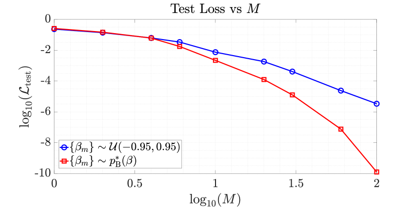
Therefore, the derived optimal probability distribution for the reservoir weights can provide up to $4$ orders of magnitude improvement in the test loss at higher reservoir sizes, indicating a huge performance improvement that can be achieved without any additional training complexity. Note that in the simulation of a simple system such as a first-order IIR system, it would take a model of a significantly larger size, i.e., reservoir with many more neurons to start observing the overfitting effect in the test loss $\mathcal{L}_{\mathrm{test}}$.

V-D Interconnected Reservoir

In order to validate our finding from Sec. III-D that interconnections between neurons in the reservoir is equivalent to a non-interconnected reservoir with modified input and output weights matrices, we replicate the evaluations of Sec. V-C, but with a non-diagonal $\mathbf{W}_{\mathrm{res}}$, i.e., with random and sparse interconnections between the reservoir neurons. The sparsity of connections is controlled via the hyperparameter ‘sparsity’ (denoted as $\kappa$) which represents the probability of each element of $\mathbf{W}_{\mathrm{res}}$ being $0$. Furthermore, the spectral radius of $\mathbf{W}_{\mathrm{res}}$ is set to $0.95$, i.e., $\max|\rho(\mathbf{W}_{\mathrm{res}})|=0.95$ for the cases of random and sparsely interconnected reservoirs.

Figure 12: Training loss versus reservoir size $M$ under finite training samples for ESN with random interconnections between neurons.

Figure 13: Test loss versus reservoir size $M$ under finite training samples for ESN with random interconnections between neurons.

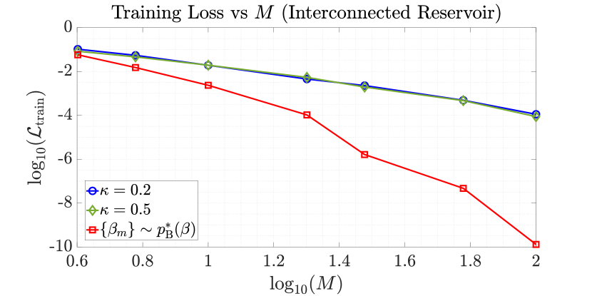
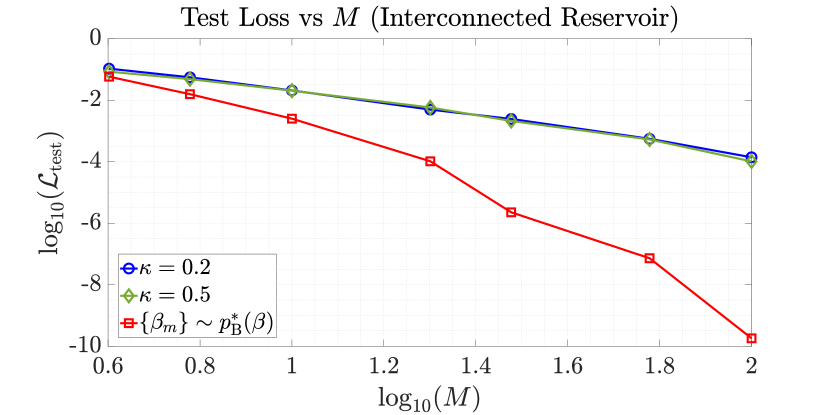
From both Fig. 12 and Fig. 13, we can observe that the training and test losses for the ESN using the optimally sampled reservoir weights outperform the ESN model initialized using state-of-the-art practice by a similar margin as with the non-interconnected reservoir. At higher reservoir sizes, e.g., $M=100$, we can see a gain of up to $6$ orders of magnitude in the test loss with optimally sampled $\{\beta_{m}\}$. Additionally, for a fixed spectral radius, a change in the sparsity of the reservoir from $\kappa=0.2$ to $\kappa=0.5$ does not result in an observable change in the trends of the training and the test losses. These evaluations confirm our hypothesis from Sec. III-D that random interconnections between neurons do not accrue additional performance gain and the test loss with random interconnections is still lower bounded by the test loss achieved with optimally sampled reservoir weights.

V-E Simulating Higher Order IIR Systems

Although the optimal distribution for the reservoir weights has been derived under the scenario of simulating a first-order IIR system, we empirically show that it holds for simulation of a general higher order IIR system as well. This is an important outcome, implying the possibility of extension of the main result derived in this paper to more general LTI systems. We simulate an IIR system given by $H(z)=\frac{1}{1+\sum_{k=1}^{K_{\mathrm{den}}}a_{k}z^{-k}}$, with $K_{\mathrm{den}}=\{3,5\}$. For this evaluation, we use a short sequence length of $L=10$ samples and $N_{p}=1$ sequence for training and $N_{d}=10$ sequences for test. The training and test losses are evaluated across $10^{4}$ Monte-Carlo simulations. The coefficients $\{a_{k}\}\in\mathbb{R}$ of the denominator are chosen such that the poles of $H(z)$ are strictly contained within $(-1,1)$ in order to realize a stable IIR system. Note that a distribution for $\{a_{k}\}$ is induced by first specifying a known distribution namely, $\mathcal{U}(-0.95,0.95)$ for the roots of $1+\sum_{k=1}^{K_{\mathrm{den}}}a_{k}z^{-k}=0$. This is unlike the scenario in the first-order system ($K_{\mathrm{den}}=1$) where the distribution for the aforementioned root and the coefficient is the same. The monotonically decreasing trend expected in the training loss with increasing reservoir size $M$ is empirically validated for both the $3$-rd and the $5$-th order IIR systems, as seen in Fig. 14 and Fig. 15 respectively.

Figure 14: Training loss versus reservoir size $M$ under finite training samples for ESN simulating a $3$-rd order IIR system.

Figure 15: Training loss versus reservoir size $M$ under finite training samples for ESN simulating a $5$-th order IIR system.

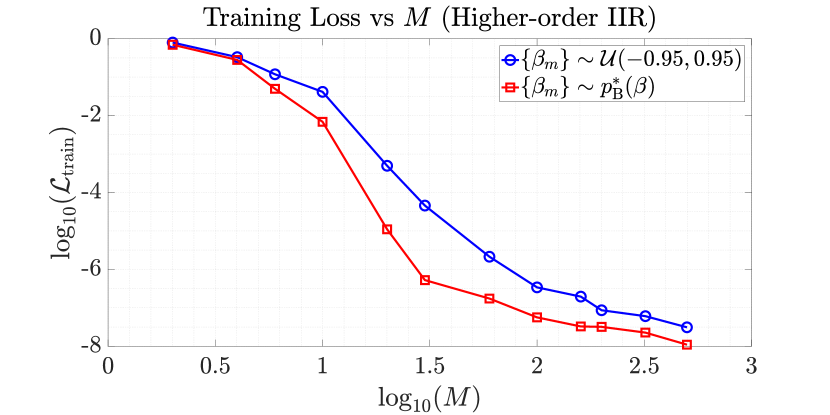
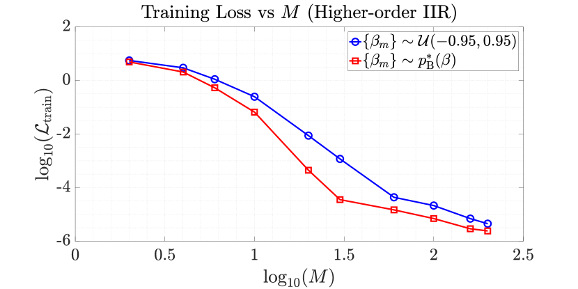
The corresponding test loss curves are also plotted in Fig. 16 and Fig. 17 respectively. We observe empirically that $\mathcal{L}_{\mathrm{test}}$ is minimized at approximately $M=120$, beyond which the ESN model starts to overfit, as evidenced by the plateauing $\mathcal{L}_{\mathrm{test}}$ for the $3$-th order IIR system (Fig. 16) and the increasing $\mathcal{L}_{\mathrm{test}}$ for the $5$-th order IIR system (Fig. 17).

Figure 16: Test loss versus reservoir size $M$ under finite training samples for ESN simulating a $3$-rd order IIR system.

Figure 17: Test loss versus reservoir size $M$ under finite training samples for ESN simulating a $5$-th order IIR system.

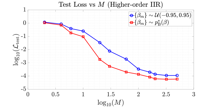
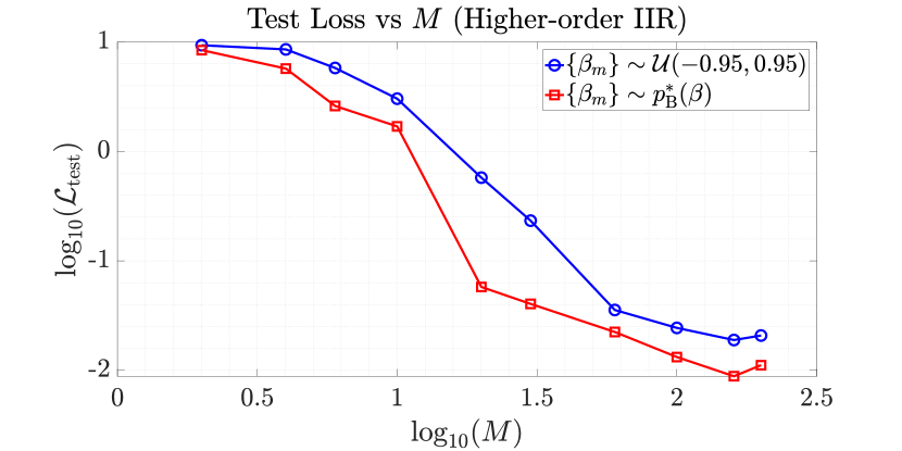
While the improvement in the test loss with the optimally sampled $\{\beta_{m}\}$ is not multiple orders of magnitude, it is still on average (across $M$) $50\%$ lower than for $\{\beta_{m}\}$ sampled from $\mathcal{U}(-0.95,0.95)$. This demonstrates the extensible nature of the optimal distribution derived for the first-order IIR to a higher order IIR system.

VI Conclusion and Future Work

In this work, we have introduced a clear signal processing approach to understand the echo state network (ESN), a powerful architecture of the Reservoir Computing (RC) family, which belongs to the broader class of recurrent neural networks (RNNs). Employing the linear ESN to simulate a simple linear time-invariant (LTI) system, we provide a complete analytical characterization of the optimal probability distribution function (PDF) that can be used initialize the ESN’s reservoir weights, which are otherwise initialized from a pre-determined arbitrary distribution and left untrained in state-of-the-art practice. Numerical evaluations demonstrate the optimality of the derived distribution by showing a gain of up to $4$ orders of magnitude in both the training and test losses at higher reservoir sizes. This indicates the practical applicability and performance gains that can be realized by virtue of the analysis in this work when applying ESNs to simulate a general LTI system. Extension of this analysis to complex-weighted ESNs and an analysis of the benefit of nonlinear activation will be part of future investigation. Additionally, derivation of the optimal reservoir weights distribution for the wireless channel equalization task given statistical knowledge of the channel is also part of future work.

Appendix A Proof of Lemma 1

Proof.

Substituting $\alpha^{*}=\frac{1}{2}(\beta_{1}+\beta_{2})$ in Eq. (23) and the substitution $\beta_{1}=\beta-\Delta$ and $\beta_{2}=\beta+\Delta$, we can arrive at the following expression after some manipulation,

$$\varepsilon_{(2)}^{(\mathrm{mid})} =\frac{\Delta^{4}}{\big{(}1+\beta^{4}-\beta^{2}(2+\Delta^{2})\big{)}^{2}},$$

$$=\frac{\Delta^{4}}{(1-\beta^{2})^{4}\left(1-\frac{2\beta^{2}\Delta^{2}}{(1-\beta^{2})^{2}}+\frac{\beta^{4}\Delta^{4}}{(1-\beta^{2})^{4}}\right)}.$$ (48)

To perform a Taylor series expansion up to the second power for the term $C_{4}^{(\mathrm{mid})}\overset{\mathrel{\raisebox{-0.43057pt}{\scalebox{0.8}[0.6]{$\vartriangle$}}}}{=}\frac{1}{\left(1-\frac{2\beta^{2}\Delta^{2}}{(1-\beta^{2})^{2}}+\frac{\beta^{4}\Delta^{4}}{(1-\beta^{2})^{4}}\right)}$, recall the Taylor series expansion for $\frac{1}{1+x}$ for $x\ll 1$ given by

$$\frac{1}{1+x}\approx 1-x+x^{2}+O(x^{3}).$$ (49)

Applying this to $C_{4}^{(\mathrm{mid})}$, we obtain

$$C_{4}^{(\mathrm{mid})} \approx 1-\left(\frac{\beta^{4}\Delta^{4}}{(1-\beta^{2})^{4}}-\frac{2\beta^{2}\Delta^{2}}{(1-\beta^{2})^{2}}\right)$$

$$+\left(\frac{\beta^{4}\Delta^{4}}{(1-\beta^{2})^{4}}-\frac{2\beta^{2}\Delta^{2}}{(1-\beta^{2})^{2}}\right)^{2},$$

$$=1+\frac{2\beta^{2}\Delta^{2}}{(1-\beta^{2})^{2}}+\frac{3\beta^{4}\Delta^{4}}{(1-\beta^{2})^{4}}+O(\Delta^{6}).$$ (50)

Using this approximation in Eq. (48), we get the result in Lemma 1,

$$\varepsilon_{(2)}^{(\mathrm{mid})}=\frac{1}{(1-\beta^{2})^{4}}\Delta^{4}+O(\Delta^{6}).$$ (51)

∎

Appendix B Proof of Lemma 2

Proof.

With the substitutions $\beta_{1}=\beta-\Delta$, $\beta_{2}=\beta+\Delta$ and a sequence of algebraic manipulations, we can arrive at the following expression for the derivative of the neighborhood error w.r.t. $\alpha$, evaluated at $\alpha_{(\mathrm{mid})}\overset{\mathrel{\raisebox{-0.43057pt}{\scalebox{0.8}[0.6]{$\vartriangle$}}}}{=}\frac{1}{2}(\beta_{1}+\beta_{2})=\beta$,

$$\frac{\partial\varepsilon_{(2)}}{\partial\alpha}\bigg{\rvert}_{\alpha=\alpha_{(\mathrm{mid})}}=\frac{4\beta(1-\beta^{2}+\Delta^{2})}{\big{(}(1-\beta^{2})^{2}-\beta^{2}\Delta^{2}\big{)}^{3}}\Delta^{4}.$$ (52)

Since a power series expansion for $\frac{\partial\varepsilon_{(2)}}{\partial\alpha}\big{\rvert}_{\alpha=\alpha_{(\mathrm{mid})}}$ in terms of $\Delta$ is required, we obtain a Taylor series expansion for the term $\frac{1}{\left((1-\beta^{2})^{2}-\beta^{2}\Delta^{2}\right)^{3}}$ as follows. First, expand

$$\frac{1}{\big{(}(1-\beta^{2})^{2}-\beta^{2}\Delta^{2}\big{)}^{3}}$$

$$=\frac{1}{(1-\beta^{2})^{6}\bigg{(}1-\frac{\beta^{6}\Delta^{6}}{(1-\beta^{2})^{6}}+\frac{3\beta^{4}\Delta^{4}}{(1-\beta^{2})^{4}}-\frac{3\beta^{2}\Delta^{2}}{(1-\beta^{2})^{2}}\bigg{)}}.$$ (53)

Next, we perform an expansion for the term

$$C_{6}^{(\mathrm{bound})}\overset{\mathrel{\raisebox{-0.43057pt}{\scalebox{0.8}[0.6]{$\vartriangle$}}}}{=}\frac{1}{1+\bigg{(}\frac{3\beta^{4}\Delta^{4}}{(1-\beta^{2})^{4}}-\frac{3\beta^{2}\Delta^{2}}{(1-\beta^{2})^{2}}-\frac{\beta^{6}\Delta^{6}}{(1-\beta^{2})^{6}}\bigg{)}},$$ (54)

using the Taylor series $\frac{1}{1+x}\approx 1-x$, for small $x$. Thus, we get

$$C_{6}^{(\mathrm{bound})}\approx 1+\frac{3\beta^{2}\Delta^{2}}{(1-\beta^{2})^{2}}-\frac{3\beta^{4}\Delta^{4}}{(1-\beta^{2})^{4}}+\frac{\beta^{6}\Delta^{6}}{(1-\beta^{2})^{6}}.$$ (55)

Simplifying Eq. (52), we get

$$\frac{\partial\varepsilon_{(2)}}{\partial\alpha}\bigg{\rvert}_{\alpha=\alpha_{(\mathrm{mid})}} =\frac{4\beta(1-\beta^{2})\Delta^{4}+4\beta\Delta^{6}}{(1-\beta^{2})^{6}}C_{6}^{(\mathrm{bound})}.$$ (56)

Substituting with the Taylor expansion for $C_{6}^{(\mathrm{bound})}$ from Eq. (55), we get

$$\frac{\partial\varepsilon_{(2)}}{\partial\alpha}\bigg{\rvert}_{\alpha=\alpha_{(\mathrm{mid})}}\approx\bigg{(}\frac{4\beta(1-\beta^{2})\Delta^{4}+4\beta\Delta^{6}}{(1-\beta^{2})^{6}}\bigg{)}$$

$$\times\bigg{(}1+\frac{3\beta^{2}\Delta^{2}}{(1-\beta^{2})^{2}}-\frac{3\beta^{4}\Delta^{4}}{(1-\beta^{2})^{4}}+\frac{\beta^{6}\Delta^{6}}{(1-\beta^{2})^{6}}\bigg{)},$$

$$=\frac{4\beta}{(1-\beta^{2})^{5}}\Delta^{4}+O(\Delta^{6}),$$ (57)

yielding the result of Lemma 2. ∎

References

- [1] I. Goodfellow, Y. Bengio, and A. Courville, Deep Learning. MIT Press, 2016.
- [2] K. He, X. Zhang, S. Ren, and J. Sun, “Deep Residual Learning for Image Recognition,” in 2016 IEEE Conf. on Comput. Vis. Patt. Recog. (CVPR), June 2016, pp. 770–778.
- [3] A. Graves, A. Mohamed, and G. Hinton, “Speech Recognition with Deep Recurrent Neural Networks,” in 2013 IEEE Intl. Conf. Acoustics, Speech and Signal Process., May 2013, pp. 6645–6649.
- [4] D. Bahdanau, K. Cho, and Y. Bengio, “Neural Machine Translation by Jointly Learning to Align and Translate,” in 3rd Intl. Conf. on Learn. Rep., ICLR 2015, San Diego, CA, USA, May 7-9, 2015, Conference Track Proceedings, 2015.
- [5] K. Funahashi and Y. Nakamura, “Approximation of dynamical systems by continuous time recurrent neural networks,” Neur. Net., vol. 6, no. 6, pp. 801 – 806, 1993.
- [6] M. M. Agüero-Torales, J. I. Abreu Salas, and A. G. López-Herrera, “Deep learning and multilingual sentiment analysis on social media data: An overview,” Applied Soft Computing, vol. 107, p. 107373, 2021.
- [7] K. Cho, B. van Merriënboer, C. Gulcehre, D. Bahdanau, F. Bougares, H. Schwenk, and Y. Bengio, “Learning Phrase Representations using RNN Encoder–Decoder for Statistical Machine Translation,” in Proceedings of the 2014 Conference on Empirical Methods in Natural Language Processing (EMNLP). Association for Computational Linguistics, Oct. 2014, pp. 1724–1734.
- [8] D. Güera and E. J. Delp, “Deepfake Video Detection Using Recurrent Neural Networks,” in 2018 15th IEEE International Conference on Advanced Video and Signal Based Surveillance (AVSS), 2018, pp. 1–6.
- [9] B. Zhao, X. Li, and X. Lu, “CAM-RNN: Co-Attention Model Based RNN for Video Captioning,” IEEE Transactions on Image Processing, vol. 28, no. 11, pp. 5552–5565, 2019.
- [10] S. S. Mosleh, L. Liu, C. Sahin, Y. R. Zheng, and Y. Yi, “Brain-Inspired Wireless Communications: Where Reservoir Computing Meets MIMO-OFDM,” IEEE Trans. Neural Netw. Learn. Syst., vol. 29, no. 10, pp. 4694–4708, 2018.
- [11] B. Peng, E. Alcaide, Q. Anthony, A. Albalak, S. Arcadinho, H. Cao, X. Cheng, M. Chung, M. Grella, K. K. GV, X. He, H. Hou, P. Kazienko, J. Kocon, J. Kong, B. Koptyra, H. Lau, K. S. I. Mantri, F. Mom, A. Saito, X. Tang, B. Wang, J. S. Wind, S. Wozniak, R. Zhang, Z. Zhang, Q. Zhao, P. Zhou, J. Zhu, and R.-J. Zhu, “RWKV: Reinventing RNNs for the Transformer Era,” 2023.
- [12] R. Pascanu, T. Mikolov, and Y. Bengio, “On the difficulty of training recurrent neural networks,” in Intl. Conf. on Machine Learning, 2013, pp. 1310–1318.
- [13] P. Werbos, “Backpropagation Through Time: What It Does and How to Do It,” Proceedings of the IEEE, vol. 78, no. 10, pp. 1550–1560, 1990.
- [14] S. Hochreiter and J. Schmidhuber, “Long Short-Term Memory,” Neural Computation, vol. 9, no. 8, pp. 1735–1780, 11 1997.
- [15] Y. Bengio, P. Simard, and P. Frasconi, “Learning Long-Term Dependencies with Gradient Descent is Difficult,” IEEE Transactions on Neural Networks, vol. 5, no. 2, pp. 157–166, 1994.
- [16] S. Hochreiter and J. Schmidhuber, “LSTM can Solve Hard Long Time Lag Problems,” in Advances in Neural Information Processing Systems, M. Mozer, M. Jordan, and T. Petsche, Eds., vol. 9. MIT Press, 1996.
- [17] A. Sherstinsky, “Fundamentals of Recurrent Neural Network (RNN) and Long Short-Term Memory (LSTM) network,” Physica D: Nonlinear Phenomena, vol. 404, p. 132306, 2020.
- [18] C. Gallicchio, A. Micheli, and P. Tiňo, “Randomized Recurrent Neural Networks,” in The European Symposium on Artificial Neural Networks, 2018.
- [19] M. Lukoševičius and H. Jaeger, “Reservoir computing approaches to recurrent neural network training,” Computer Science Review, vol. 3, no. 3, pp. 127–149, 2009.
- [20] M. Lukoševičius, A Practical Guide to Applying Echo State Networks. Springer Berlin Heidelberg, 2012, pp. 659–686.
- [21] X. Hinaut and P. F. Dominey, “On-Line Processing of Grammatical Structure Using Reservoir Computing,” in Artificial Neural Networks and Machine Learning – ICANN 2012, A. E. P. Villa, W. Duch, P. Érdi, F. Masulli, and G. Palm, Eds. Berlin, Heidelberg: Springer Berlin Heidelberg, 2012, pp. 596–603.
- [22] A. Juven and X. Hinaut, “Cross-Situational Learning with Reservoir Computing for Language Acquisition Modelling,” in 2020 International Joint Conference on Neural Networks (IJCNN), 2020, pp. 1–8.
- [23] A. Jalalvand, G. Van Wallendael, and R. Van De Walle, “Real-Time Reservoir Computing Network-Based Systems for Detection Tasks on Visual Contents,” in 2015 7th International Conference on Computational Intelligence, Communication Systems and Networks, 2015, pp. 146–151.
- [24] W.-J. Wang, Y. Tang, J. Xiong, and Y.-C. Zhang, “Stock market index prediction based on reservoir computing models,” Expert Systems with Applications, vol. 178, p. 115022, 2021.
- [25] Z. Zhou, L. Liu, and H.-H. Chang, “Learning for Detection: MIMO-OFDM Symbol Detection Through Downlink Pilots,” IEEE Trans. Wireless Commun., vol. 19, no. 6, pp. 3712–3726, 2020.
- [26] Z. Zhou, L. Liu, S. Jere, J. Zhang, and Y. Yi, “RCNet: Incorporating Structural Information Into Deep RNN for Online MIMO-OFDM Symbol Detection With Limited Training,” IEEE Trans. Wireless Commun., vol. 20, no. 6, pp. 3524–3537, 2021.
- [27] J. Xu, Z. Zhou, L. Li, L. Zheng, and L. Liu, “RC-Struct: A Structure-based Neural Network Approach for MIMO-OFDM Detection,” IEEE Transactions on Wireless Communications, pp. 1–1, 2022.
- [28] H.-P. Ren, H.-P. Yin, C. Bai, and J.-L. Yao, “Performance Improvement of Chaotic Baseband Wireless Communication Using Echo State Network,” IEEE Transactions on Communications, vol. 68, no. 10, pp. 6525–6536, 2020.
- [29] H.-H. Chang, L. Liu, and Y. Yi, “Deep Echo State Q-Network (DEQN) and Its Application in Dynamic Spectrum Sharing for 5G and Beyond,” IEEE Transactions on Neural Networks and Learning Systems, vol. 33, no. 3, pp. 929–939, 2022.
- [30] F. Da Ros, S. M. Ranzini, H. Bülow, and D. Zibar, “Reservoir-Computing Based Equalization With Optical Pre-Processing for Short-Reach Optical Transmission,” IEEE Journal of Selected Topics in Quantum Electronics, vol. 26, no. 5, pp. 1–12, 2020.
- [31] H. Dai and Y. K. Chembo, “Classification of IQ-Modulated Signals Based on Reservoir Computing With Narrowband Optoelectronic Oscillators,” IEEE Journal of Quantum Electronics, vol. 57, no. 3, pp. 1–8, 2021.
- [32] R. Shafin, L. Liu, V. Chandrasekhar, H. Chen, J. Reed, and J. C. Zhang, “Artificial Intelligence-Enabled Cellular Networks: A Critical Path to Beyond-5G and 6G,” IEEE Wireless Communications, vol. 27, no. 2, pp. 212–217, 2020.
- [33] G. Montavon, A. Binder, S. Lapuschkin, W. Samek, and K.-R. Müller, Layer-Wise Relevance Propagation: An Overview. Cham: Springer International Publishing, 2019, pp. 193–209.
- [34] R. Shwartz-Ziv and N. Tishby, “Opening the Black Box of Deep Neural Networks via Information,” 2017.
- [35] S. M. Lundberg and S.-I. Lee, “A Unified Approach to Interpreting Model Predictions,” in Proceedings of the 31st International Conference on Neural Information Processing Systems, ser. NIPS’17. Red Hook, NY, USA: Curran Associates Inc., 2017, p. 4768–4777.
- [36] D. Baehrens, T. Schroeter, S. Harmeling, M. Kawanabe, K. Hansen, and K.-R. Müller, “How to explain individual classification decisions,” J. Mach. Learn. Res., vol. 11, p. 1803–1831, aug 2010.
- [37] M. C. Ozturk, D. Xu, and J. C. Príncipe, “Analysis and Design of Echo State Networks,” Neural Comput., vol. 19, no. 1, p. 111–138, 2007.
- [38] E. Bollt, “On explaining the surprising success of reservoir computing forecaster of chaos? The universal machine learning dynamical system with contrast to VAR and DMD,” Chaos, vol. 31, p. 013108, 2021.
- [39] A. G. Hart, J. L. Hook, and J. H. Dawes, “Echo State Networks trained by Tikhonov least squares are L2() approximators of ergodic dynamical systems,” Physica D: Nonlinear Phenomena, vol. 421, p. 132882, 2021.
- [40] A. Haluszczynski and C. Räth, “Good and bad predictions: Assessing and improving the replication of chaotic attractors by means of reservoir computing,” Chaos, vol. 29, no. 10, p. 103143, 2019.
- [41] T. L. Carroll, “Optimizing memory in reservoir computers,” Chaos, vol. 32, no. 2, p. 023123, 2022.
- [42] S. Jere, R. Safavinejad, and L. Liu, “Theoretical Foundation and Design Guideline for Reservoir Computing-based MIMO-OFDM Symbol Detection,” IEEE Transactions on Communications, pp. 1–1, 2023.
- [43] L. Gonon, L. Grigoryeva, and J.-P. Ortega, “Risk Bounds for Reservoir Computing,” Jour. Mach. Learn. Res., vol. 21, no. 240, pp. 1–61, 2020.
- [44] S. Jere, R. Safavinejad, L. Zheng, and L. Liu, “Channel Equalization Through Reservoir Computing: A Theoretical Perspective,” IEEE Wireless Communications Letters, vol. 12, no. 5, pp. 774–778, 2023.
- [45] A. Edelman and N. R. Rao, “Random matrix theory,” Acta Numerica, vol. 14, p. 233–297, 2005.
- [46] H. Akaike, Information Theory and an Extension of the Maximum Likelihood Principle. New York, NY: Springer New York, 1998, pp. 199–213.
- [47] P. Stoica and Y. Selen, “Model-Order Selection: A review of information criterion rules,” IEEE Signal Processing Magazine, vol. 21, no. 4, pp. 36–47, 2004.
- [48] C. P. Robert and G. Casella, Monte Carlo Statistical Methods. Springer, 1999, vol. 2.
- [49] B. S. Caffo, J. G. Booth, and A. C. Davison, “Empirical supremum rejection sampling,” Biometrika, vol. 89, no. 4, pp. 745–754, 12 2002.