Contrastive Self-Supervised Learning Based Approach for Patient Similarity: A Case Study on Atrial Fibrillation Detection from PPG Signal

Abstract

In this paper, we propose a novel contrastive learning based deep learning framework for patient similarity search using physiological signals. We use a contrastive learning based approach to learn similar embeddings of patients with similar physiological signal data. We also introduce a number of neighbor selection algorithms to determine the patients with the highest similarity on the generated embeddings. To validate the effectiveness of our framework for measuring patient similarity, we select the detection of Atrial Fibrillation (AF) through photoplethysmography (PPG) signals obtained from smartwatch devices as our case study. We present extensive experimentation of our framework on a dataset of over 170 individuals and compare the performance of our framework with other baseline methods on this dataset.

1 Introduction

Recent advances in wearable devices and the adaptation of these devices in the medical domain for timely and continuous monitoring have led to the generation of a huge volume of patient data as a part of electronic health records (EHR). With the availability of a vast amount of data, patient similarity based diagnostics and analysis have become increasingly crucial in the medical domain. Patient similarity has been applied in several medical domains including generic diagnostics [1, 2, 3, 4], Alzheimer’s disease [5], coronary artery disease [6], precision medicine [7, 8, 9], mortality prediction [10], etc.

The key intuition of EHR based patient similarity comes from the observation that patients suffering from the same diseases or abnormalities generally preserve a common pattern. Among the sources of EHR, sensor based physiological data is one of the most common ones in recent days. For example, ECG signals are used to detect arrhythmia & cardiovascular diseases, EEG signals are used for BCI (Brain Computer Interface), EMG signals are used for speech, prosthesis, & rehabilitation robotics, PPG signals are used for atrial fibrillation (AF), etc. [11] Let us consider an example involving PPG signals. Figure 1 shows the PPG signals for a normal sinus rhythm and atrial fibrillation. Here, varying pulse-to-pulse intervals can be noticed in the PPG signals for AF, and such abnormal patterns in signals can be utilized by similarity based learning. For example, according to Figure 1, if we want to find similar individuals as the one with signal $a$, then similarity based model will return persons with signals $b$ and $c$ as the two most similar ones. Similarly, if signal $d$ is from a query patient, then such model will return patients with signals $e$ and $f$ as the results.

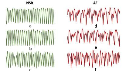
Figure 1: PPG Signals: Normal Sinus Rhythm (NSR) vs Atrial Fibrillation (AF).

Finding the similarities between pair-wise patients is one of the fundamental problems in the medical sector, and this problem has been approached by researchers from different angles over the years [12]. However, most of the research relies on static data (patient background, age, weight, etc.) and longitudinal clinical events data (visit date of patients, symptoms, disease, diagnosis, etc.) [10, 1, 4], rather than physiological signals. Since incorporating time-series data like physiological signals with similarity-based learning is not trivial [13], it has not been explored heavily in the medical domain. However, with the increasing popularity of wearable sensors in capturing physiological signals (e.g., ECG, EEG, etc.), a few recent works have also focused on signal based similarities [14, 15]. The presence of noise, motion artifacts due to a lot of sensors, and missing values in some cases, still continue to pose major challenges in such research.

Researchers have also extensively studied time series data for a number of years. The recent availability of physiological signals in the medical domain has encouraged researchers to apply algorithms and models to such signals. Though statistical methods were primarily used, they suffer from low-adaptivity and robustness due to variations of signals in patients and devices. They also suffer from high time complexity. One such popular algorithm for time series classification, named HIVE-COTE, has good accuracy [16]. However, its time complexity of $O(n^{2}\cdot l^{4})$ (where $n$ is the number of time series in the dataset and $l$ is the length of a time series) makes its use in real-time settings very limited and impractical.

To overcome this challenge, machine learning based approaches have been introduced that can replace the threshold-based statistical detection [17, 18] . However, conventional machine learning based approaches need extraction of pre-selected features which can be labor-intensive. Recent advancements in deep learning is taking over the analysis of time-series data. For example, the deep residual network architecture  [19] can achieve the almost same accuracy of HIVE-COTE. Moreover, such deep neural network (DNN) based methods eliminate the requirement of feature engineering and selection. As a result, there have been multiple works using DNN on time-series data [20, 21, 22, 23, 24]. DNNs on time-series data have been extensively applied to physiological signals in recent times [25, 26, 27, 28, 29, 30]. Though all physiological signals are time-series data, they have different collection processes, features and applications. For example, EMG signal analysis for gesture, speech recognition [31, 28], EEG signal analysis for brain computer interface [32, 33], ECG signal analysis for cardiovascular diseases [26, 27], EOG analysis for eye movements [34, 35]. Among all these signals, ECG signal is the most studied one due to its least noisy nature.

However, the above existing works that used deep learning models in physiological signals are based on supervised learning and hence, suffer from data annotation problems. In the health domain, manual annotation is very time-consuming and expensive which makes it difficult to annotate a large dataset manually. So, obtaining a dataset with 100% accurate ground-truth labeling is not feasible in the physiological signal dataset domain. Moreover, mislabelled training samples affecting the performance and biasing supervised classifiers is a very common issue in this domain.

To solve the above problems, in this paper, we propose a contrastive self-supervised deep learning method for physiological signal based patient similarity detection. Intuitively, contrastive learning is a representation learning framework that learns similar embeddings of positive pairs of samples (e.g., two similar samples in some sense) and ensures that the embeddings of negative pairs (e.g., two very different samples) are different from each other [36].

In our case, the signals from patients of the same disease can be considered as positive pairs and vice versa. Thus, we can use more pairs of samples in self-supervised learning (SSL) than in supervised learning – which can mitigate the data annotation issue of physiological datasets. For example, if a dataset has $n$ and $m$ labeled signals for sick and healthy patients, respectively, a supervised learning method can use $(n+m)$ samples at most, whereas our contrastive learning based approach can use $(n\times m)$ pairs to train the model. Recent work [37] showed that SSL is more robust to dataset imbalance.

In this paper, we first present a generic self-supervised contrastive learning framework for finding physiological signal based patient similarity. To demonstrate the efficacy of our proposed framework, we applied and tested our framework in detecting Atrial Fibrillation (AF)  since it is the most common arrhythmia [38]. Most of the existing approaches to detect AF are based on ECG signals [39, 26, 40, 41, 42]. But such approaches are not applicable to prolonged monitoring with low cost. This motivated us to focus on Photoplethysmography (PPG) signals. Most of the wearables (e.g. smartwatches) nowadays are equipped with low-cost easy-to-implement optical sensors that can measure the PPG signals. As a result, it is possible to monitor patients continuously by analyzing the PPG signals.

PPG signals have been recently used for AF detection using various approaches [18, 43, 44, 17] including DL techniques  [45, 46, 47, 48, 49].  [29] adapted ResNeXt architecture for 1D PPG data to detect AF. However, such a computationally heavy model might not be suitable for low-resource devices which is one of the sole reasons for using PPG signals.  [50] proposed an unsupervised transfer learning through convolutional denoising autoencoders (CADE). But for transfer learning, the parent model they used was trained using supervised learning. Though AF detection using PPG signal is promising, it has major challenges (e.g., noise, motion artifact, intra, and inter-patient variability, etc.). [30] leveraged Bayesian deep learning to mitigate the noise issue PPG signals and provided an uncertainty estimate of the prediction. All the prior works had to use some kind of supervised learning which requires manual labeling of individual signals. To the best of our knowledge, we are the first to use self-supervised contrastive learning on PPG signals to detect AF. In summary, the main contributions of this paper are as follows:

• We propose a novel Contrastive Learning based approach, namely SimSig, for patient similarity search on physiological signal data.

• As a self-supervised approach, SimSig can work on a partially-labeled dataset, which overcomes a key bottleneck of labeling medical data records.

• Our detailed experimental study with real datasets shows that SimSig has achieved better accuracy in AF detection than the existing state-of-the-art approaches.

2 Methods: SimSig

In this section, we first give a formal definition of our problem, and then discuss the key concept of contrastive learning. After that, we provide the formulation of our contrastive learning based patient similarity framework, which we named SimSig. Then we present the network architecture, the training details of SimSig and neighbor selection algorithms.

2.1 Problem Definition

Suppose $P=\{P_{1}^{1},\dots,P_{1}^{n_{1}},\dots,P_{i}^{1},\dots,P_{i}^{n_{i}},\dots,P_{N}^{1},\dots,\\ P_{N}^{n_{N}}\}$ for $i=1,2,...,N$ is a patient database of $N$ individuals, each having multiple time series signal segments obtained from sensors where patient $i$ has $n_{i}$ segments. Each segment $P_{i}^{j}$ for $j=1,2,...,n_{i}$ is of length $l$, i.e., $P_{i}^{j}\in\mathbb{R}^{l}$. Our goal is to predict label $y\in\{0,1\}$ for a query individual $Q$ based on the labels from the patient database.

2.2 Contrastive Representation Learning

Contrastive representation learning or in short, Contrastive learning is a popular form of self-supervised learning that encourages augmentations of the same input to have more similar representations or embeddings compared to augmentations or embeddings from different inputs. The key idea of contrastive representation learning is to contrast semantically similar and dissimilar pairs of data points to make the representation of similar pairs closer, and those of dissimilar pairs more orthogonal by minimizing the contrastive loss [51, 52].

2.3 Model Architecture of SimSig

Inspired by the framework proposed by [52] named SimCLR, we design our network adopting some of the core components of SimCLR. The SimCLR learns representation by maximizing the agreements between different augmentations of similar categories of examples. Since we intend to learn the similarity within the segments (portions) of physiological signals of the same type of patients, we maximize agreements between segments from the same individual and examine how this helps to learn similarities across patients with similar physiological signals. Our adopted framework comprises the following three major components as demonstrated in Figure 2:

• A neural network based encoder $f(.)$ to extract representation vectors from signal segments. We pass input vector $P_{i}^{k}$ to obtain representation vector $h_{i}^{k}=f(P_{i}^{k})$. In our case, we use 1D ResNext50 as our encoder architecture.

• A small neural network projection head $g(.)$ similar to [52] that maps the representation vectors generated by the encoder on which contrastive loss is applied. An MLP with one hidden layer is used to obtain $z_{i}^{k}=g(h_{i}^{k})$

• A contrastive loss function to apply on $z_{i}^{k}$’s. We consider custom defined contrastive loss functions below.

Contrastive Loss Functions

We consider two contrastive loss functions: NT-Xent loss as defined in [52] and another variant of it proposed by us. We name the latter one NT-Xent Multi loss.

In the NT-Xent loss shown in Equation 1, the same sample is augmented to produce a pair, and the model is trained to increase the similarity between the pair. In our case, we only sample two segments from the same individual in a batch and consider them as a pair.

$$l_{\alpha}=-log\frac{exp(sim(z_{\alpha},z_{\beta})/\tau)}{\sum_{\gamma=1}^{N}[1_{[\gamma\notin\{\alpha,\beta\}]}exp(sim(z_{\alpha},z_{\gamma})/\tau)]}$$ (1)

Here, $\beta$ is a segment such that $\beta\neq\alpha$ and $ind(\beta)=ind(\alpha)$. $\tau$ is a hyper-parameter. Note that the similarity function (cosine similarity in our case) has been applied on the output of the projection head i.e. $z$’s. Finally, the total loss is aggregated as:

$$L=\sum_{i=1}^{N}l_{i}$$ (2)

However, this imposes a limit on the batch size. Hence, we designed another loss function, NT-Xent Multi loss. For the NT-Xent Multi loss, we randomly sample a minibatch of $K$ examples. In these $K$ examples, say there are examples from $N_{K}$ unique individuals ($N_{K}\leq K$) and the loss function for $\alpha$-th sample is defined as:

$$l_{\alpha}=-log\frac{\sum_{\beta=1}^{K}[1_{[ind(\beta)=ind(\alpha)]}exp(sim(z_{\alpha},z_{\beta})/\tau)]}{\sum_{\gamma=1}^{K}[1_{[ind(\gamma)\neq ind(\alpha)]}exp(sim(z_{\alpha},z_{\gamma})/\tau)]}$$ (3)

Here, $\tau$ is a hyper-parameter. In summary, the numerator part inside the logarithm function is the summation of exponential similarities between segments from the same individual, which we consider as positive samples. The denominator part is the summation of exponential similarities between segments from different individuals which we consider as negative samples. Finally, the total loss function is defined like the previous one as:

$$L=\sum_{i=1}^{N}l_{i}$$ (4)

The similarity learning network architecture is demonstrated in Figure 2. The encoder network, 1D ResNext50 (in this case), takes 1D signal segments and generates the corresponding embeddings of size 1024. We denote the embedding of $k$-th segment of the $i$-th individual as $h_{i}^{k}$. The embeddings: $h_{i}^{k}$’s are then passed to the projection layer to generate $z_{i}^{k}$’s. The projection layer consists of a linear layer followed by a ReLU activation, then another linear layer to generate $z_{i}^{k}$.

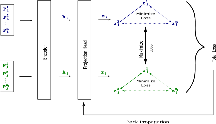
Figure 2: SimSig Contrastive Representation Learning Training Pipeline

2.4 Inference Phase

In this phase, our framework works in two major steps as demonstrated in Figure 3. First, it generates the embeddings of signal segments from an individual using the encoder model we trained earlier using contrastive representation learning. After that, we perform a number of similarity measurements and neighbor selections with the embeddings of individuals we have in our database. Based on the neighbors, we label a new individual.

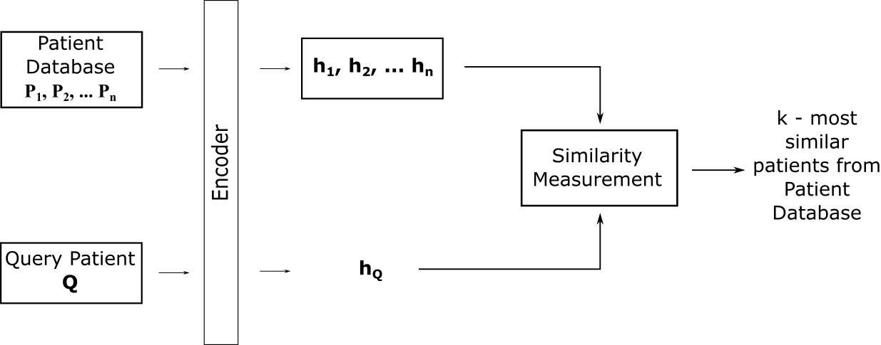
Figure 3: Patient Similarity Detection using Our Model

Once the network is trained by minimizing the contrastive loss, we generate the embeddings of training samples to be later used for patient similarity. We refer to this as Patient Database. Note that in order to achieve the best performance according to [52], we use $h_{i}^{j}$’s for the embeddings. We similarly obtain embedding $q_{i}^{j}$’s for time series segments from a query patient, $Q$ whose label we want to infer.

2.5 Neighbor Selection

From the SimSig Encoder model, we get an embedding vector for each segment. We keep the embeddings of individuals from the training set that we refer to as the Patient Database. During the evaluation, we apply different metrics for this distance calculation between a query individual and an individual from the Patient Database. Figure 3 represents the generic model of distance calculation. In Figure 3, the $P_{i}$ represents the patients with id $i$. The $i$-th patient has $n_{i}$ number of segments of PPG signal, and each segment is represented by ${P}_{i}^{j}$, where $i$ is the patient id and $j$, is the $j$-th segment of a signal. After feeding these segments to our encoder, we get the embedding vector $h_{i}^{j}$ for each ${P}_{i}^{j}$.

To calculate the pair-wise distance between a query patient and a patient from the database, we first calculate the distance between every pair of embedding vectors where one is from a query patient and the other one is from a patient in the patient database. For example, to calculate the distance (or the similarity in our context) from query patient $Q$ to the $i$-th patient $P_{i}$ in our patient database, the $h_{Q}^{j}$ embedding vectors are multiplied with the embeddings of the $i$-th patient i.e. $h_{i}^{k}$’s in the patient database.

After that, we used different metrics to calculate the distance between the two individuals We denote $d_{i}$ as the final distance between the query patient and $i$-th patient where $i$ represents the id of the patient in the patient database with whom the distance is to be calculated. Thus, for a query patient, we calculate the final distance $d_{i}$’s for each patient in our Patient Database where $i=[1,N]$, $N=$ number of individuals in the database. Consider $P_{i}$ to be an individual in database with $n_{i}$ signal embeddings $h_{i}^{1},h_{i}^{2},....,h_{i}^{n_{i}}$. Let $Q$ be a test individual with $M$ embeddings $h_{Q}^{1},h_{Q}^{2},....,h_{Q}^{M}$. We denote $d_{i}^{j,m}$ to be the distance between $h_{i}^{j}$ and $h_{Q}^{m}$. We experimented with the following distance calculation criteria to measure the distance between the signals of two individuals:

Overall Min Distance

Here we consider the minimum distance between two segments where each one is from a separate individual as the distance between those two individuals. We first calculate the pairwise cosine distances between every pair of segments between $P_{i}$ and Q. We calculate $n_{i}\times m$ cosine distances and finally we take distance $d_{i}$ to be:

$$d_{i}=min(d_{i}^{1,1},d_{i}^{1,2},\dots,d_{i}^{j,m},\dots,d_{i}^{n_{i},m})$$

as the distance between the query individual Q and $P_{i}$ with respect to their signal similarity. We get $N$ such distances for the whole database. Finally, we choose the $k$ nearest individuals to $Q$ in terms of distance. We label $Q$ as AF if the majority of the $k$ neighbors are AF individuals, otherwise Non-AF.

Average Min Distance

In this case we consider the average of all the distances between all possible pairs of segments where each one is from a separate individual as the distance between those two individuals. We calculate the $d_{i}^{j,m}$’s similarly to Overall Min Distance criteria. Then finally we take,

$$d_{i}=average(d_{i}^{1,1},d_{i}^{1,2},\dots,d_{i}^{j,m},\dots,d_{i}^{n_{i},m})$$

to be the distance between the query individual Q and $P_{i}$ with respect to their signal similarity. Finally, we label $Q$ as previously discussed.

Weighted Average Min Distance

We also consider a weighted version of the average min distance by weighting the individual label with $1/{d_{i}^{j,m}}^{2}$ i.e. the inverse of the squared distance.

Pct Min Distance

In this setting for an individual, we calculate all possible pairs of distances with every segment from all other neighbors i.e. individuals in the database. Among the neighbors we consider the closest neighbors to be the individuals who have the most number of segments with distances that are below a certain value, which we call the radius. We first choose a hyper-parameter, radius, $r$. Then we calculate a count for every individual in the database. The count for individual $i$ in the database is defined as:

We take the top $k$ individuals with the highest $C_{i}$ values. We infer the label of $Q$ similarly to the aforementioned ones.

3 Experiments

In our experiment, we have selected the Atrial Fibrillation (AF) detection problem to be our case study. In this section, we first give the description of the AF detection problem followed by the description of the dataset that we use as an example to apply our framework. After that we provide the implementation details and training environment configurations for two Simsig versions. Then we define some of the evaluation metrics we use in our experiment. We have run extensive experiments with all the configurations by varying the hyper-parameters, and report them in the Result section.

3.1 AF Detection Problem

Given a set of PPG signal segments of an individual, we want to detect whether the person has atrial fibrillation (AF) or not. Atrial Fibrillation (AF) is a type of abnormality characterized by irregular beating of the two upper chambers of the heart.

For our case-study, we will detect negative (Non-AF) or positive (Atrial Fibrillation) for the individual whose signal segments from $Q$ and our time series data consists of PPG signals obtained from wearable sensors.

3.2 Dataset

We have used the largest publicly available dataset, which we refer to as the Stanford Wearable Photoplethysmography Dataset for training our model and evaluating with the state-of-the-art.  [50] made this dataset public with their work DeepBeat. The dataset contains signal segments collected using wrist-worn wearable devices. There are more than 500K segments from a total of 175 individuals (108 AF subjects and 67 non-AF subjects), each with duration of 25s sampled at 128 Hz and later downsampled to 32 Hz. The starting timestamp of each segment is also provided along with the dataset.

The dataset includes three categories of signal labels, labeled as Poor, Good, and Excellent. However, only a portion of these labels were assigned by humans; the remaining labels were generated by a model trained on the human-labeled portion, resulting in imprecise labels in the dataset. This can cause downstream models to be susceptible to error propagation, as demonstrated in [30].

Table 1: Distribution of the Revised Dataset from [30]

Set	#Individuals	#Samples	#AF Samples	#Non-AF Samples	#AF Individuals	#Non-AF Individuals	Size ratio
Train	132	108171	41511	66660	82	50	0.698
Validation	20	22294	8310	13984	12	8	0.144
Test	23	24579	9703	14876	14	9	0.159

The provided dataset also has some distribution issues present in the original train, validation, test split. This distribution issue has been addressed and a proper redistribution has been provided by [30]. Hence, we adapt the distribution from [30] with a split of 70% as train, 15% as validation, and 15% as test sets where no subject is shared among different sets and all overlapping signal segments from the validation and test sets are removed using the description of the split provided by [30]. The distribution is shown in Table 1

3.3 Implementation Details

The cost function in Equation 4 is optimized by minibatch gradient descent. We have used the Adam optimizer variant since it gives the best performance in our experiments. We sample 512 segments for a minibatch that might contain multiple samples from the same individual and minimize the total loss value according to it. Figure 2 represents the training pipeline for similarity learning. Note that the loss values among $z_{i}^{j}$’s of similar individuals are minimized while loss with other individuals is maximized.

We implement the training pipeline for training our model in PyTorch [53]. We selected $batch\_size=512$ for NT-Xent Multi loss configuration and trained for 50 epochs with a learning rate of $1x10^{-3}$ with Adam [54] as the optimizer using an i7-7700 workstation with 32GB of RAM, and a GTX 1070 GPU for a day.

3.4 Evaluation Metrics and Baselines

We have employed a diverse set of metrics, such as Recall (Sensitivity), Specificity (True Negative Rate, TNR), Precision (Positive Predictive Value, PPV), F1-score, and Accuracy, to evaluate various models. The formal expressions of these metrics are as follows.

$$Recall =\frac{TP}{TP+FN}$$

$$Specificity =\frac{TN}{TN+FP}$$

$$Precision =\frac{TP}{TP+FP}$$

$$F1 =\frac{2*(Precision*Recall)}{Precision+Recall}$$

$$Accuracy =\frac{TP+TN}{TP+TN+FP+FN}$$

In this context, TP (True Positive) refers to the number of positive individuals (AF patients) that the model correctly identified, TN (True Negative) refers to the number of negative individuals (non-AF patients) that the model correctly identified, FP (False Positive) refers to the number of individuals that the model incorrectly classified as positive, and FN (False Negative) refers to the number of individuals that the model incorrectly classified as negative.

Most of the works in this field have been limited to segment wise prediction whereas our work is on individual-level. [29, 50] have been the state-of-the-art works for predicting AF/Non-AF for a PPG segment. We adapted their approach to predict AF/Non-AF for an individual. For an individual, if more than half of the segments results into AF predictions for these models, we label the individual as AF.

4 Results

In this section, we present the results of our experiments. First, we analyze SimSig for various neighbor sizes and configuration parameters.

4.1 Model performance and Ablation Study

First, we present the results on the validation set for the configurations with the topmost performances in Table 2 with five different sub-tables separately for different values of the neighbor size $k$. We have set the value of hyper-parameter, $\tau=0.5$ for both loss functions NT-Xent and NT-Xent Multi loss.

Table 2: Performance of SimSig on Validation for different configurations

((a)) For k=3

Model Loss Function	Configuration	Sensitivity	Specificity	Precision	F1	Accuracy
NT-Xent	Average Min Distance	0.167	1	1	0.286	0.5
	Overall Min Distance	0.667	0.75	0.8	0.727	0.7
	Pct Min Distance	0.333	1	1	0.5	0.6
NT-Xent Multi	Average Min Distance	0.917	1	1	0.957	0.95
	Overall Min Distance	0.917	0.75	0.846	0.88	0.85
	Pct Min Distance	0.5	1	1	0.667	0.7

((b)) For k=5

Model Loss Function	Configuration	Sensitivity	Specificity	Precision	F1	Accuracy
NT-Xent	Average Min Distance	0.167	1	1	0.286	0.5
	Overall Min Distance	0.667	0.75	0.8	0.727	0.7
	Pct Min Distance	0.333	1	1	0.5	0.6
NT-Xent Multi	Average Min Distance	0.917	1	1	0.957	0.95
	Overall Min Distance	0.833	0.75	0.833	0.833	0.8
	Pct Min Distance	0.5	1	1	0.667	0.7

((c)) For k=7

Model Loss Function	Configuration	Sensitivity	Specificity	Precision	F1	Accuracy
NT-Xent	Average Min Distance	0.083	1	1	0.154	0.45
	Overall Min Distance	0.667	0.75	0.8	0.727	0.7
	Pct Min Distance	0.333	1	1	0.5	0.6
NT-Xent Multi	Average Min Distance	0.917	1	1	0.957	0.95
	Overall Min Distance	0.833	0.75	0.833	0.833	0.8
	Pct Min Distance	0.5	1	1	0.667	0.7

((d)) For k=9

Model Loss Function	Configuration	Sensitivity	Specificity	Precision	F1	Accuracy
NT-Xent	Average Min Distance	0.083	1	1	0.154	0.45
	Overall Min Distance	0.667	0.75	0.8	0.727	0.7
	Pct Min Distance	0.333	1	1	0.5	0.6
NT-Xent Multi	Average Min Distance	0.833	1	1	0.909	0.9
	Overall Min Distance	0.75	0.75	0.818	0.783	0.75
	Pct Min Distance	0.583	1	1	0.737	0.75

((e)) For k=11

Model Loss Function	Configuration	Sensitivity	Specificity	Precision	F1	Accuracy
NT-Xent	Average Min Distance	0.167	1	1	0.286	0.5
	Overall Min Distance	0.75	0.75	0.818	0.783	0.75
	Pct Min Distance	0.333	1	1	0.5	0.6
NT-Xent Multi	Average Min Distance	0.833	1	1	0.909	0.9
	Overall Min Distance	0.75	0.75	0.818	0.783	0.75
	Pct Min Distance	0.583	1	1	0.737	0.75

We have tried each configuration by varying neighbor size, $k$ to be 3, 5, 7, 9, and 11, using both loss functions NT-Xent and NT-Xent Multi. The table  2 shows performances separately for all the distance metrics we defined earlier for each configuration. However, weighted versions of Average Min and Overall Min performed exactly the same as the unweighted versions. Hence, we did not report their performance separately.

For the network using NT-Xent loss, we can observe from Table 2 that the neighbor selection criteria ‘Overall Min Distance’ performs the best for all of $k=3,5,7,9~{}and~{}11$. While for the network using NT-Xent Multi loss, the neighbor selection criteria ‘Average Min Distance’ shows the best performance for different $k$ values. Hence, we select the ‘Overall Min Distance’ metric for the network using NT-Xent loss and ‘Average Min Distance’ metric for the network using NT-Xent Multi loss.

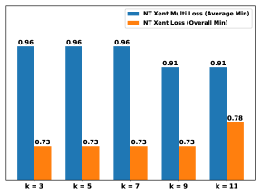
Figure 4: Selection of best neighbor size k

Figure 4 represents the best F1 score for both losses considering the best configuration for each of them. We can observe that NT-Xent Multi loss with ‘Average Min Distance’ outperforms NT-Xent loss with ‘Overall Min Distance’ for every value of $k$. Also for $k=3,5,7$, NT-Xent Multi loss with ‘Average Min Distance‘ provides a similar performance of $0.96$ F1 score which drops down to $0.91$ with higher $k$ values. Therefore, we choose $k=7$ for the ‘Average Min Distance’ metric since it is expected to have a better prediction and more confidence to practitioners because of taking a decision from a higher number of neighbors from the Patient Database. Hence, we choose NT-Xent Multi loss as our SimSig loss function with ‘Average Min Distance’ as the neighbor selection metric with neighbor size $k=7$ to compare it with other baseline methods in the next subsection.

4.2 Comparison with baseline methods

We compare the performance of the SimSig on the test set with two other baseline methods, namely ResNext [29] and DeepBeat [50], that have been adapted to work with individuals. Since these two baselines predict on signal segments, in order to generate individual-wise AF/Non-AF labels we considered an individual as AF if he/she receives more AF labeled signal segments than Non-AF labeled signal segments by the model. We report the results in Table 3.

Table 3: Comparison of Simsig with other baseline models on Revised Stanford Wearable Photoplethysmography Dataset

	Sensitivity	Specificity	Precision	F1	Accuracy
[29] ResNext	0.714	0.889	0.909	0.8	0.783
[50] (Deepbeat)	0.857	0.778	0.857	0.857	0.826
[50] (DeepBeat (Excellent))	0.6	0.714	0.75	0.667	0.647
[50] (DeepBeat (Non-Poor))	0.75	0.714	0.818	0.783	0.737
Simsig (NT-Xent Multi loss, Average Min Distance, $k=7$)	0.929	0.667	0.813	0.867	0.826

Table 3 demonstrates the performance of different methods considering sensitivity (recall), specificity, precision, F1-score, and accuracy of SimSig with those of other baseline methods on the test set of the dataset. We present the performance of SimSig with the configuration of ‘Average Min Distance’ ($k=7$) with NT-Xent Multi loss since it yields the best performance on the validation set. We also show the performance metrics of DeepBeat [50] on three settings based on their signal quality prediction.

We observe that SimSig with the mentioned configuration outperforms other baseline models for overall metrics like F1-score and accuracy. Compared to [29], SimSig has 6.7% higher F1-score and 4.3% higher accuracy. When compared to Deepbeat [50], SimSig outperforms it by 1-20% for F1-score and up to 17.9% for accuracy depending on its settings.

5 Conclusion

In this paper, we proposed a novel framework to learn the similarity between patients from their physiological signals using self-supervised contrastive learning and neighbor selection. Our main focus was to address the data annotation issue that causes the supervised approaches to suffer. As a case study, we have selected the Atrial Fibrillation detection problem from the photoplethysmography signal. We have thoroughly experimented with our framework on the dataset for our case study varying several hyper-parameters: neighbor selection criteria, neighbor size, etc. From the comparison with other baseline methods, we find that our framework for finding patient similarity performed substantially better than those.

6 Code Availability

Trained weights and relevant source codes of SimSig are publicly available at this github link:
https://github.com/Subangkar/Simsig

References

- [1] Zheng Jia, Xian Zeng, Huilong Duan, Xudong Lu, and Haomin Li. A patient-similarity-based model for diagnostic prediction. International journal of medical informatics, 135:104073, 2020.
- [2] Suresh Pokharel, Guido Zuccon, Xue Li, Chandra Prasetyo Utomo, and Yu Li. Temporal tree representation for similarity computation between medical patients. Artificial Intelligence in Medicine, 108:101900, 2020.
- [3] Araek Tashkandi, Ingmar Wiese, and Lena Wiese. Efficient in-database patient similarity analysis for personalized medical decision support systems. Big data research, 13:52–64, 2018.
- [4] Ping Zhang, Fei Wang, Jianying Hu, and Robert Sorrentino. Towards personalized medicine: leveraging patient similarity and drug similarity analytics. AMIA Summits on Translational Science Proceedings, 2014:132, 2014.
- [5] Yuang Shi, Chen Zu, Mei Hong, Luping Zhou, Lei Wang, Xi Wu, Jiliu Zhou, Daoqiang Zhang, and Yan Wang. Asmfs: Adaptive-similarity-based multi-modality feature selection for classification of alzheimer’s disease. Pattern Recognition, 126:108566, 2022.
- [6] Márton Kolossváry, Thomas Mayrhofer, Maros Ferencik, Júlia Karády, Neha J Pagidipati, Svati H Shah, Michael G Nanna, Borek Foldyna, Pamela S Douglas, Udo Hoffmann, et al. Are risk factors necessary for pretest probability assessment of coronary artery disease? a patient similarity network analysis of the promise trial. Journal of Cardiovascular Computed Tomography, 2022.
- [7] Sherry-Ann Brown. Patient similarity: emerging concepts in systems and precision medicine. Frontiers in physiology, 7:561, 2016.
- [8] Shraddha Pai and Gary D Bader. Patient similarity networks for precision medicine. Journal of molecular biology, 430(18):2924–2938, 2018.
- [9] Enea Parimbelli, Simone Marini, Lucia Sacchi, and Riccardo Bellazzi. Patient similarity for precision medicine: A systematic review. Journal of biomedical informatics, 83:87–96, 2018.
- [10] Joon Lee, David M Maslove, and Joel A Dubin. Personalized mortality prediction driven by electronic medical data and a patient similarity metric. PloS one, 10(5):e0127428, 2015.
- [11] Tania Pereira, Nate Tran, Kais Gadhoumi, Michele M Pelter, Duc H Do, Randall J Lee, Rene Colorado, Karl Meisel, and Xiao Hu. Photoplethysmography based atrial fibrillation detection: a review. NPJ digital medicine, 3(1):3, 2020.
- [12] Ahmed Allam, Matthias Dittberner, Anna Sintsova, Dominique Brodbeck, and Michael Krauthammer. Patient similarity analysis with longitudinal health data. arXiv preprint arXiv:2005.06630, 2020.
- [13] Mohammad M. Masud, Kadhim Hayawi, Sujith Samuel Mathew, Ahmed Dirir, and Muhsin Cheratta. Effective patient similarity computation for clinical decision support using time series and static data. In Proceedings of the Australasian Computer Science Week Multiconference, pages 1–8, 2020.
- [14] Filippo Maria Bianchi, Lorenzo Livi, Karl Øyvind Mikalsen, Michael Kampffmeyer, and Robert Jenssen. Learning representations for multivariate time series with missing data using temporal kernelized autoencoders. arXiv preprint arXiv:1805.03473, 2018.
- [15] Fons J Wesselius, Mathijs S van Schie, Natasja MS De Groot, and Richard C Hendriks. An accurate and efficient method to train classifiers for atrial fibrillation detection in ecgs: Learning by asking better questions. Computers in Biology and Medicine, 143:105331, 2022.
- [16] Anthony Bagnall, Jason Lines, Aaron Bostrom, James Large, and Eamonn Keogh. The great time series classification bake off: a review and experimental evaluation of recent algorithmic advances. Data mining and knowledge discovery, 31(3):606–660, 2017.
- [17] Sibylle Fallet, Mathieu Lemay, Philippe Renevey, Célestin Leupi, Etienne Pruvot, and Jean-Marc Vesin. Can one detect atrial fibrillation using a wrist-type photoplethysmographic device? Medical & biological engineering & computing, 57:477–487, 2019.
- [18] Tim Schäck, Yosef Safi Harb, Michael Muma, and Abdelhak M Zoubir. Computationally efficient algorithm for photoplethysmography-based atrial fibrillation detection using smartphones. In 2017 39th Annual International Conference of the IEEE Engineering in Medicine and Biology Society (EMBC), pages 104–108. IEEE, 2017.
- [19] Zhiguang Wang, Weizhong Yan, and Tim Oates. Time series classification from scratch with deep neural networks: A strong baseline. In 2017 International joint conference on neural networks (IJCNN), pages 1578–1585. IEEE, 2017.
- [20] Henry Friday Nweke, Ying Wah Teh, Mohammed Ali Al-Garadi, and Uzoma Rita Alo. Deep learning algorithms for human activity recognition using mobile and wearable sensor networks: State of the art and research challenges. Expert Systems with Applications, 105:233–261, 2018.
- [21] Zhengping Che, Yu Cheng, Shuangfei Zhai, Zhaonan Sun, and Yan Liu. Boosting deep learning risk prediction with generative adversarial networks for electronic health records. In 2017 IEEE International Conference on Data Mining (ICDM), pages 787–792. IEEE, 2017.
- [22] Hassan Ismail Fawaz, Germain Forestier, Jonathan Weber, Lhassane Idoumghar, and Pierre-Alain Muller. Evaluating surgical skills from kinematic data using convolutional neural networks. In Medical Image Computing and Computer Assisted Intervention–MICCAI 2018: 21st International Conference, Granada, Spain, September 16-20, 2018, Proceedings, Part IV 11, pages 214–221. Springer, 2018.
- [23] Yi Zheng, Qi Liu, Enhong Chen, Yong Ge, and J Leon Zhao. Time series classification using multi-channels deep convolutional neural networks. In Web-Age Information Management: 15th International Conference, WAIM 2014, Macau, China, June 16-18, 2014. Proceedings 15, pages 298–310. Springer, 2014.
- [24] Chien-Liang Liu, Wen-Hoar Hsaio, and Yao-Chung Tu. Time series classification with multivariate convolutional neural network. IEEE Transactions on industrial electronics, 66(6):4788–4797, 2018.
- [25] Oliver Faust, Yuki Hagiwara, Tan Jen Hong, Oh Shu Lih, and U Rajendra Acharya. Deep learning for healthcare applications based on physiological signals: A review. Computer methods and programs in biomedicine, 161:1–13, 2018.
- [26] U Rajendra Acharya, Hamido Fujita, Oh Shu Lih, Yuki Hagiwara, Jen Hong Tan, and Muhammad Adam. Automated detection of arrhythmias using different intervals of tachycardia ecg segments with convolutional neural network. Information sciences, 405:81–90, 2017.
- [27] Jen Hong Tan, Yuki Hagiwara, Winnie Pang, Ivy Lim, Shu Lih Oh, Muhammad Adam, Ru San Tan, Ming Chen, and U Rajendra Acharya. Application of stacked convolutional and long short-term memory network for accurate identification of cad ecg signals. Computers in biology and medicine, 94:19–26, 2018.
- [28] Michael Wand and Jürgen Schmidhuber. Deep neural network frontend for continuous emg-based speech recognition. In Interspeech, pages 3032–3036, 2016.
- [29] Yichen Shen, Maxime Voisin, Alireza Aliamiri, Anand Avati, Awni Hannun, and Andrew Ng. Ambulatory atrial fibrillation monitoring using wearable photoplethysmography with deep learning. In Proceedings of the 25th ACM SIGKDD International Conference on Knowledge Discovery & Data Mining, pages 1909–1916, 2019.
- [30] Sarkar Snigdha Sarathi Das, Subangkar Karmaker Shanto, Masum Rahman, Md Saiful Islam, Atif Hasan Rahman, Mohammad M Masud, and Mohammed Eunus Ali. Bayesbeat: Reliable atrial fibrillation detection from noisy photoplethysmography data. Proceedings of the ACM on Interactive, Mobile, Wearable and Ubiquitous Technologies, 6(1):1–21, 2022.
- [31] Weidong Geng, Yu Du, Wenguang Jin, Wentao Wei, Yu Hu, and Jiajun Li. Gesture recognition by instantaneous surface emg images. Scientific reports, 6(1):36571, 2016.
- [32] Robin Tibor Schirrmeister, Jost Tobias Springenberg, Lukas Dominique Josef Fiederer, Martin Glasstetter, Katharina Eggensperger, Michael Tangermann, Frank Hutter, Wolfram Burgard, and Tonio Ball. Deep learning with convolutional neural networks for eeg decoding and visualization. Human brain mapping, 38(11):5391–5420, 2017.
- [33] U Rajendra Acharya, Shu Lih Oh, Yuki Hagiwara, Jen Hong Tan, and Hojjat Adeli. Deep convolutional neural network for the automated detection and diagnosis of seizure using eeg signals. Computers in biology and medicine, 100:270–278, 2018.
- [34] Li-Huan Du, Wei Liu, Wei-Long Zheng, and Bao-Liang Lu. Detecting driving fatigue with multimodal deep learning. In 2017 8th International IEEE/EMBS Conference on Neural Engineering (NER), pages 74–77. IEEE, 2017.
- [35] Xuemin Zhu, Wei-Long Zheng, Bao-Liang Lu, Xiaoping Chen, Shanguang Chen, and Chunhui Wang. Eog-based drowsiness detection using convolutional neural networks. In 2014 International Joint Conference on Neural Networks (IJCNN), pages 128–134. IEEE, 2014.
- [36] HaoChen Jeff Z., Wei Colin, and Tengyu Ma. Understanding deep learning algorithms that leverage unlabeled data, part 2: Contrastive learning. http://ai.stanford.edu/blog/understanding-contrastive-learning/, 2022. Accessed: 2023-03-04.
- [37] Hong Liu, Jeff Z HaoChen, Adrien Gaidon, and Tengyu Ma. Self-supervised learning is more robust to dataset imbalance. arXiv preprint arXiv:2110.05025, 2021.
- [38] Christopher RC Wyndham. Atrial fibrillation: the most common arrhythmia. Texas Heart Institute Journal, 27(3):257, 2000.
- [39] Jinghao Niu, Yongqiang Tang, Zhengya Sun, and Wensheng Zhang. Inter-patient ecg classification with symbolic representations and multi-perspective convolutional neural networks. IEEE journal of biomedical and health informatics, 24(5):1321–1332, 2019.
- [40] Yong Xia, Naren Wulan, Kuanquan Wang, and Henggui Zhang. Detecting atrial fibrillation by deep convolutional neural networks. Computers in biology and medicine, 93:84–92, 2018.
- [41] Zhenjie Yao, Zhiyong Zhu, and Yixin Chen. Atrial fibrillation detection by multi-scale convolutional neural networks. In 2017 20th international conference on information fusion (Fusion), pages 1–6. IEEE, 2017.
- [42] Chan Yuan, Yan Yan, Lin Zhou, Jingwen Bai, and Lei Wang. Automated atrial fibrillation detection based on deep learning network. In 2016 IEEE International Conference on Information and Automation (ICIA), pages 1159–1164. IEEE, 2016.
- [43] Pak-Hei Chan, Chun-Ka Wong, Yukkee C Poh, Louise Pun, Wangie Wan-Chiu Leung, Yu-Fai Wong, Michelle Man-Ying Wong, Ming-Zher Poh, Daniel Wai-Sing Chu, and Chung-Wah Siu. Diagnostic performance of a smartphone-based photoplethysmographic application for atrial fibrillation screening in a primary care setting. Journal of the American Heart Association, 5(7):e003428, 2016.
- [44] Jinseok Lee, Bersain A Reyes, David D McManus, Oscar Mathias, and Ki H Chon. Atrial fibrillation detection using a smart phone. In 2012 Annual International Conference of the IEEE Engineering in Medicine and Biology Society, pages 1177–1180. IEEE, 2012.
- [45] Alireza Aliamiri and Yichen Shen. Deep learning based atrial fibrillation detection using wearable photoplethysmography sensor. In 2018 IEEE EMBS International Conference on Biomedical & Health Informatics (BHI), pages 442–445. IEEE, 2018.
- [46] Maxime Voisin, Yichen Shen, Alireza Aliamiri, Anand Avati, Awni Hannun, and Andrew Ng. Ambulatory atrial fibrillation monitoring using wearable photoplethysmography with deep learning. arXiv preprint arXiv:1811.07774, 2018.
- [47] Supreeth P Shashikumar, Amit J Shah, Gari D Clifford, and Shamim Nemati. Detection of paroxysmal atrial fibrillation using attention-based bidirectional recurrent neural networks. In Proceedings of the 24th ACM SIGKDD International Conference on Knowledge Discovery & Data Mining, pages 715–723, 2018.
- [48] Soonil Kwon, Joonki Hong, Eue-Keun Choi, Euijae Lee, David Earl Hostallero, Wan Ju Kang, Byunghwan Lee, Eui-Rim Jeong, Bon-Kwon Koo, Seil Oh, et al. Deep learning approaches to detect atrial fibrillation using photoplethysmographic signals: algorithms development study. JMIR mHealth and uHealth, 7(6):e12770, 2019.
- [49] Igor Gotlibovych, Stuart Crawford, Dileep Goyal, Jiaqi Liu, Yaniv Kerem, David Benaron, Defne Yilmaz, Gregory Marcus, and Yihan Li. End-to-end deep learning from raw sensor data: Atrial fibrillation detection using wearables. arXiv preprint arXiv:1807.10707, 2018.
- [50] Jessica Torres-Soto and Euan A Ashley. Multi-task deep learning for cardiac rhythm detection in wearable devices. NPJ digital medicine, 3(1):1–8, 2020.
- [51] Aaron Van den Oord, Yazhe Li, and Oriol Vinyals. Representation learning with contrastive predictive coding. arXiv e-prints, pages arXiv–1807, 2018.
- [52] Ting Chen, Simon Kornblith, Mohammad Norouzi, and Geoffrey Hinton. A simple framework for contrastive learning of visual representations. In International conference on machine learning, pages 1597–1607. PMLR, 2020.
- [53] Adam Paszke, Sam Gross, Francisco Massa, Adam Lerer, James Bradbury, Gregory Chanan, Trevor Killeen, Zeming Lin, Natalia Gimelshein, Luca Antiga, et al. Pytorch: An imperative style, high-performance deep learning library. Advances in neural information processing systems, 32, 2019.
- [54] Diederik P Kingma and Jimmy Ba. Adam: A method for stochastic optimization. arXiv preprint arXiv:1412.6980, 2014.