A State-Space Perspective on Modelling and
Inference for Online Skill Rating

Abstract

This paper offers a comprehensive review of the main methodologies used for skill rating in competitive sports. We advocate for a state-space model perspective, wherein players’ skills are represented as time-varying, and match results serve as the sole observed quantities. The state-space model perspective facilitates the decoupling of modeling and inference, enabling a more focused approach highlighting model assumptions, while also fostering the development of general-purpose inference tools. We explore the essential steps involved in constructing a state-space model for skill rating before turning to a discussion on the three stages of inference: filtering, smoothing and parameter estimation. Throughout, we examine the computational challenges of scaling up to high-dimensional scenarios involving numerous players and matches, highlighting approximations and reductions used to address these challenges effectively. We provide concise summaries of popular methods documented in the literature, along with their inferential paradigms and introduce new approaches to skill rating inference based on sequential Monte Carlo and finite state-spaces. We close with numerical experiments demonstrating a practical workflow on real data across different sports.

1 Introduction

In the quantitative analysis of competitive sports, a fundamental task is to estimate the skills of the different agents (‘players’) involved in a given competition based on the outcome of pairwise comparisons (‘matches’) between said players, often in an online setting. Skill estimation facilitates the prediction of various relevant outcomes of subsequent matches, which can then be applied towards high-level decision-making for the competition, including player seeding, fair team matching, and more. There are several established approaches to the task of skill estimation, including among others the Bradley-Terry model (Bradley and Terry, 1952), the Elo rating system (Elo, 1978), the Glicko rating system (Glickman, 1999), and TrueSkill (Herbrich et al., 2006) each with various levels of complexity and varying degrees of statistical motivation.

Skill rating is of paramount importance in the world of competitive sports as it serves as a foundational tool for assessing and comparing the abilities of players and how they vary over time. By accurately quantifying skill levels, skill rating systems enable fair and balanced competition, inform strategic decision-making, and enhance the overall sporting level. Popular skill rating systems applications include chess (FIDE, 2023), online gaming (Herbrich et al., 2006), education (Pelánek, 2016), tennis (Kovalchik, 2016) and team-based sports like football (Hvattum and Arntzen, 2010), basketball (Štrumbelj and Vračar, 2012) and many more (Stefani, 2011). Skill ratings not only facilitate player ranking, but also serve as a basis for dynamic matchmaking and player seeding, ensuring that competitive matches are engaging and well-matched. Moreover, in professional sports, skill rating plays a pivotal role in talent scouting and gauging overall performance, providing data-driven insights for coaches, analysts, bettors and fanatics. As technology and statistical methodologies continue to advance, skill rating systems are expected to evolve further, benefiting an ever-widening spectrum of sports and competitive domains.

In this work, we argue for an explicitly model-based, statistical approach to this task, centred around state-space models. We model the skills of the players in the competition as time-varying, and we model the outcomes of matches between players as indirect observations of these skills. Such models are often left implicit in the presentation of popular approaches to the skill estimation task. Our viewpoint is that by emphasising the role of the underlying models, users can more easily incorporate additional structure into their estimation routines. Moreover, this emphasis encourages the decoupling of the algorithmic aspects of estimation from the modeling aspects, which again affords additional flexibility and robustness.

The paper will proceed as follows. In Section 2, we describe a high-level formalism for state-space formulations of the skill estimation problem. In Section 3, we outline the possible inference objectives for this problem and how they interact as well as the general structure of tractable inference, induced approximations and relevant complexity considerations. In Section 4, we review a variety of concrete procedures for the skill estimation problem, combining probabilistic models and inference algorithms unifying existing approaches and introducing new ones. In Section 5, we perform some numerical experiments, demonstrating and contrasting some of the varied approaches on real data. Finally, in Section 6, we conclude with a discussion on general recommendations and extensions. The paper is accompanied by a python package for reproducibility and extension of discussed techniques, found at github.com/SamDuffield/abile.

2 Model Specification

Throughout, we will use various terminology which is specific to the skill estimation problem. We will use ‘sport’ to denote a sport in the abstract (e.g. football), and will use ‘match’ to denote a specific instance of this sport being played (e.g. a match between two football teams). All matches will be contested between two competing ‘players’ (e.g. a football team is a ‘player’), one of whom is designated as the ‘home’ player, and the other as the ‘away’ player (even for sports in which there is no notion of ‘home ground’ or ‘home advantage’). A ‘competition’ refers to a specific sport, a collection of players of that sport, a set of matches between these players, and a set of results of these matches (e.g. the results of the English Premier League). Each match is also associated to a time $t\in\left[0,\infty\right)$ denoting when the match was played, which we call a ‘matchtime’.

Notationally, given an integer $N\in\operatorname{\mathbf{N}}$ we use $\left[N\right]$ for the set of integers from $1$ to $N$. The total number of players in the competition is denoted $N\in\operatorname{\mathbf{N}}$, and $K\in\operatorname{\mathbf{N}}$ denotes the total number of matches played in the competition. We order the matchtimes as $t_{1}\leqslant t_{2}\leqslant\cdots\leqslant t_{K}$ (noting that matches may take place contemporaneously). Matches are then indexed in correspondence with this ordering, i.e. match $1$ took place at time $t=t_{1}$, etc.; we also adopt the convention that $t_{0}=0$. We explicitly model the skills of all players over the full time window $[0,T]$, even if individual players may enter the competition at a later time.

We now discuss modelling choices. Our key interest is to infer the skills of players in a fixed competition, given access to the outcomes of matches which are played in that competition. We model player skills as taking values in a totally-ordered set $\mathcal{X}$, i.e. skills are treated as ordinal, with the convention that higher skill ratings are indicative of more favourable match outcomes for a player. We model match outcomes as taking values in a finite, discrete set $\mathcal{Y}$, e.g. $\mathcal{Y}=\left\{\text{draw},\text{home win},\text{away win}\right\}$, although the framework is general and can be extended to more complex scenarios. We also assume direct observation of matchtimes, who the home and away players are in a given match, and the outcome of the match.

Our model will consist of the players’ skills, and the match outcomes; we detail here the construction of the full joint likelihood. Players’ skills are allowed to vary with time, and we write $x_{t}^{i}\in\mathcal{X}$ for the skill value of the $i$th player at time $t$ and in an abuse of notation, we will also use $x_{k}^{i}$ to denote the skill value of the $i$th player at observation time $t_{k}$. We will, where possible, index skills with letters $t$ or $k$ so that the continuous/discrete nature of the time index is clear from context. For discrete time indices, we also make use of the notation $x_{0:k}$ or $y_{1:k}$ to denote the joint vector of skills or observations at discrete times.

We assume that the initial skills of the players are all drawn mutually independently of one another, i.e. for $i\in\left[N\right]$, $x_{0}^{i}\sim m_{0}^{i}$ independently for some initial distribution $m_{0}^{i}$. We also assume that the evolution of each player’s skill over time is independent of one another. We further assume that each of these evolutions is Markovian, i.e. for each $i\in\left[N\right]$, there is a semigroup of $\mathcal{X}$-valued Markov transition kernels $\left(M_{t,t^{\prime}}^{i}:t\leqslant t^{\prime}\right)$ such that for $t\leqslant t^{\prime}$,

$$x_{t^{\prime}}^{i}\mid x_{t}^{i}\sim M_{t,t^{\prime}}^{i}\left(x_{t}^{i},\cdot\right),$$

where $t,t^{\prime}$ represent matchtimes. Again, we will often abuse notation to write $M_{k,k^{\prime}}^{i}=M_{t_{k},t_{k^{\prime}}}^{i}$ with $t_{k}\leqslant t_{k^{\prime}}$ and the nature of the index clear from context.

For the $k$th match, we write $h(k),a(k)\in\left[N\right]$ for the indices of the home and away players in that match, and write $y_{k}\in\mathcal{Y}$ for the outcome of the match. We assume that given the skills of players $h(k)$ and $a(k)$ at time $t_{k}$, the match’s outcome $y_{k}$ is conditionally independent of all other player skills and match outcomes (depicted in Fig. 1), and is drawn according to some probability distribution $G_{k}\left(y_{k}\mid x_{{k}}^{h\left(k\right)},x_{{k}}^{a\left(k\right)}\right)$.

Figure 1: On the left, the conditional independence structure of an SSM. On the right, the conditional independence structure of an fSSM (1), with $N=4$ and a pairwise observation model.

Assembling these various assumptions, it follows that the joint law of all players’ skills on all matchtimes, and of all match results, is thus given by the following

$$\begin{split}\mathbf{P}\left(x_{0:K}^{\left[N\right]},y_{1:K}\right)=&\prod_{i\in\left[N\right]}\left\{m_{0}^{i}\left(x_{0}^{i}\right)\cdot\prod_{k=1}^{K}M_{{k-1},{k}}^{i}\left(x_{{k-1}}^{i},x_{{k}}^{i}\right)\right\}\\ &\cdot\prod_{k=1}^{K}G_{k}\left(y_{k}\mid x_{{k}}^{h\left(k\right)},x_{{k}}^{a\left(k\right)}\right).\end{split}$$ (1)

Some simplifications which we will make in all subsequent examples are that i) we will model the initial laws of all players’ skill as being identical across players (i.e. $m_{0}^{i}$ will not depend on $i$), ii) the dynamics of all players’ skills will also be identical across players, i.e. for $t<t^{\prime}$, we can write $M_{t,t^{\prime}}^{i}\left(x,x^{\prime}\right)=M_{t,t^{\prime}}\left(x,x^{\prime}\right)$, and iii) the observation model $G_{k}$ will not depend on $k$ (although we will still use the notation $G_{k}$ to emphasise dependence on $y_{k}$). These simplifications are made for ease of presentation, and deviations from each of these simplifications are typically straightforward to accommodate in the algorithms which we present. Such deviations are often relevant in practical scenarios, e.g. representing the off-season in seasonal sports, different match types (e.g. 3-set and 5-set tennis), and so on.

There are also a number of model features which we insist on, namely i) we insist on modeling player skills as evolving in continuous time, and ii) we insist on the possibility of observations which occur at irregularly-spaced intervals in time. We do this because these settings are of practical relevance, and because they pose particular computational challenges which deserve proper attention.

Terminologically, we use the term ‘state-space model’ (SSM) to denote a model, such as (1), in which there is an unobserved state $x$, taking values in a general space, which evolves in time according to a Markovian evolution, and is observed indirectly. We use the term ‘hidden Markov model’ (HMM) to refer to an SSM where the unobserved state $x$ takes values on a finite state space. The term factorial state-space model (fSSM, or indeed fHMM) refers to a state-space model in which the state $x$ is naturally partitioned into a collection of sub-states, each of which evolve independently of one another (Ghahramani and Jordan, 1995), see Fig. 1.

3 Inference

In this section, we discuss the problem of inference in the skill rating problem, which features of the problem one might seek to understand, and how one might go about representing these features.

3.1 Inference Objectives

Broadly speaking, inference in general state-space models tends to involve the solution of (some subset of) three related tasks, presented in (roughly) increasing order of complexity:

1. Filtering: inferring the current latent states, given the observations thus far, i.e.

   $$\mathrm{Filter}_{k}\left(x_{k}\right):=\mathbf{P}\left(x_{k}\mid y_{1:k}\right),$$

   which is closely related to prediction, i.e. for $t_{k}<t_{k+1}$

   $$\mathrm{Predict}_{k+1\mid k}\left(x_{k+1}\right)=\mathbf{P}\left(x_{k+1}\mid y_{1:k}\right).$$

2. Smoothing: inferring past latent skills, given the observations thus far, i.e. for $t_{k}\leqslant t_{k+1}\leqslant t_{K}$

   $$\mathrm{Smooth}_{k|K}\left(x_{k}\right) =\mathbf{P}\left(x_{k}\mid{y}_{1:K}\right),$$

   $$\mathrm{Smooth}_{k,k+1|K}\left(x_{k},x_{k+1}\right) =\mathbf{P}\left(x_{k},x_{k+1}\mid{y}_{1:K}\right),$$

   $$\mathrm{Smooth}_{0:K|K}\left(x_{0:K}\right) =\mathbf{P}\left(x_{0:K}\mid{y}_{1:K}\right).$$

3. Parameter Estimation: when the dynamical and/or observational structure of the model depend on unknown parameters $\theta$, one can calibrate these models based on the observed data by e.g. maximum likelihood estimation:

   $$\operatorname*{arg\,max}_{\theta\in\Theta}\mathbf{P}\left({y}_{1:K}\mid\theta\right),$$

   where $\mathbf{P}({y}_{1:K}\mid\theta)=\int\mathbf{P}\left(x_{{0:K}}^{\left[N\right]},{y}_{1:K}\mid\theta\right)\,\mathrm{d}x_{0:K}^{\left[N\right]}$. Note that for filtering and smoothing, $\theta$ is treated as constant, hence its omission from the preceding descriptions.

Depending on the application in question, each of these tasks can be of more or less interest. In our setting, because we are interested in using our model to make real-time decisions, filtering is directly relevant towards informing those decisions. However, this does not mean that we can immediately ignore the other two tasks. Firstly, without an accurate estimate of the parameters $\theta$ which govern the dynamical and observation models for our process of interest, our estimate of the filtering distribution can be badly misspecified. As a result, without incorporating some elements of parameter estimation, inference of the latent states can be quite poor. Moreover, obtaining good estimates of these model parameters tends to require developing an understanding of the full trajectory of the latent process; indeed, many algorithms for parameter estimation in SSMs require some form of access to the smoothing distribution, which in turn requires the filtering distributions. As such, the three tasks are deeply interconnected.

In Section 4, we will explicitly consider computational methods for addressing these inference objectives. For the problems considered in this paper, it is rare that the true filtering or smoothing distributions can even be represented, and as such, approximations will be adopted. It bears mentioning that the ‘richness’ of the chosen approximation will play an important role in determining how well the original inference goals are achieved. This will be treated further in Section 4.

3.2 Techniques for Filtering

We first present some generalities on algorithmic approaches to the filtering and smoothing problem, to contextualise the forthcoming developments. For a general SSM on $\mathcal{X}$ with transitions $M_{t,t^{\prime}}$ and observations $G_{k}$, the following abstract filtering recursions hold

$$\mathrm{Predict}_{k+1|k}\left(x_{k+1}\right) =\int\mathrm{Filter}_{k}\left(x_{k}\right)\cdot M_{k,k+1}\left(x_{k},x_{k+1}\right)\,\mathrm{d}x_{k},$$

$$\mathrm{Filter}_{k+1}\left(x_{k+1}\right) \propto{\mathrm{Predict}_{k+1|k}\left(x_{k+1}\right)\cdot G_{k+1}\left(x_{k+1}\right)},$$

or more suggestively,

$$\mathrm{Predict}_{k+1|k} =\mathsf{Propagate}\left(\mathrm{Filter}_{k};M_{k,k+1}\right),$$

$$\mathrm{Filter}_{k+1} =\mathsf{Assimilate}\left(\mathrm{Predict}_{k+1|k};G_{k+1}\right),$$

where we note that the operators $\mathsf{Propagate}$ and $\mathsf{Assimilate}$ act on probability measures. Note that the $\mathsf{Propagate}$ operator can also readily be applied to times which are not associated with matches; this can be useful for forecasting purposes.

The same recursions also allow for computation of the likelihood of all observations so far, using that $\mathbf{P}\left({y}_{1:k+1}\right)=\mathbf{P}\left({y}_{1:k}\right)\cdot\mathbf{P}\left(y_{k+1}\mid{y}_{1:k}\right)$ when $t_{k}\leqslant t_{k+1}$; here, the last term carries the interpretation of a predictive likelihood or in the skill-rating setting, match outcome predictions.

Various algorithms for approximate filtering have been derived by approximating each of these updates in turn. The computational cost varies depending on the algorithm being used; we will discuss these on a case-by-case basis.

3.3 Techniques for Smoothing

Similarly to filtering, there are ‘backward’ recursions which characterise the smoothing laws: if no observations occur in the interval $\left(t_{k},t_{k+1}\right)$, then

$$\mathrm{Smooth}_{k,k+1|K}\left(x_{k},x_{k+1}\right) =\frac{\mathrm{Filter}_{k}\left(x_{k}\right)\cdot M_{k,k+1}\left(x_{k},x_{k+1}\right)\cdot\mathrm{Smooth}_{k+1|K}\left(x_{k+1}\right)}{\mathrm{Predict}_{k+1|k}(x_{k+1})},$$

$$\mathrm{Smooth}_{k|K}\left(x_{k}\right) =\int\mathrm{Smooth}_{k,k+1|K}\left(x_{k},x_{k+1}\right)\,\mathrm{d}x_{k+1},$$

or

$$\mathrm{Smooth}_{k,k+1|K} =\mathsf{Bridge}\left(\mathrm{Filter}_{k},\mathrm{Smooth}_{k+1|K};M_{k,k+1}\right)$$

$$\mathrm{Smooth}_{k|K} =\mathsf{Marginalise}\left(\mathrm{Smooth}_{k,k+1|K};k\right),$$

where, as for filtering, the operators act on probability measures, and noting that $M_{k,k+1}$ is interpreted as a density, rather than as a Markov kernel. Likewise, several algorithms for approximate smoothing are built upon approximation of these recursions.

Smoothing between observation times is possible using the same approach, i.e. for $t_{k}\leqslant t_{k^{\prime}}\leqslant t_{k+1}$ where $t_{k^{\prime}}$ is not associated with an observation, we have

$$\mathrm{Smooth}_{k^{\prime},k+1|K}=\mathsf{Bridge}\left(\mathrm{Predict}_{k^{\prime}|k},\mathrm{Smooth}_{k+1|K};M_{k^{\prime},k+1}\right).$$

In general, exact implementation of any of $\left\{\mathsf{Propagate},\mathsf{Assimilate},\mathsf{Bridge},\mathsf{Marginalise}\right\}$ tends to only be possible in models with substantial conjugacy properties, due to the general difficulty of integration and representation of probability measures of even moderate complexity. If one insists on exact implementation of all of these operations, then one tends to be restricted to working with linear-Gaussian SSMs or HMMs of moderate size. As such, practical algorithms must often make approximations which restore some level of tractability to the model.

Observe also that, given the filtering distributions, the smoothing recursions require no further calls to the likelihood term $G_{k}$, which can be noteworthy in the case that the likelihood is computationally expensive or otherwise complex.

3.4 Standing Approximations and Reductions

We are interested in developing procedures for filtering, smoothing, and parameter estimation whose complexity scales well with respect to the parameters of interest for skill rating. In particular, we want to be able to process competitions involving i) many players, i.e. $N\to\infty$, and ii) many matches, i.e. $K\to\infty$. We will therefore focus on procedures for which the computational cost scales at most linearly in each of $N$ and $K$.

3.4.1 Decoupling Approximation

In seeking procedures with stable behaviour as the number of players grows, there is one approximation which seems to be near-universal in the setting of pairwise comparisons, namely that the filtering (and smoothing) distributions over all of the players’ skills are well-approximated by a decoupled representation. Using superscripts to index player-specific distributions (e.g. $\mathrm{Filter}_{k}^{i}$ denoting the filtering distribution for the skill of player $i$ at time $t_{k}$, and so on), this corresponds to the approximation

$$\mathrm{Filter}_{k}=\mathbf{P}\left(x_{k}^{\left[N\right]}\mid y_{1:k}\right) \approx\prod_{i\in\left[N\right]}\mathbf{P}\left(x_{k}^{i}\mid y_{1:k}\right)=\prod_{i\in\left[N\right]}\mathrm{Filter}_{k}^{i}$$

$$\mathrm{Smooth}_{\circ\mid K}=\mathbf{P}\left(x_{\circ}^{\left[N\right]}\mid y_{1:K}\right) \approx\prod_{i\in\left[N\right]}\mathbf{P}\left(x_{\circ}^{i}\mid y_{1:K}\right)=\prod_{i\in\left[N\right]}\mathrm{Smooth}_{\circ\mid K}^{i},$$

where we have $\circ=\left\{k\right\},\left\{k,k+1\right\}$ or $\{0:K\}$ for the various marginal and joint smoothing objectives. This approximation is largely motivated by the practical difficulty of representing large systems of correlated random variables, and is further supported by the standing assumption that players’ skills evolve independently of one another a priori.

The quality of such approximations depends heavily on the ability to control the strength of interactions between players, that is, the sensitivity of the conditional law of any one player’s skill to perturbations in any single other player’s skill. If such control is possible (which one expects for large-scale, high-frequency competitions, with weakly-informative match outcomes), then one can rigorously establish that the decoupling approximation has good fidelity to the true filtering law (Rebeschini and van Handel, 2015; Rimella and Whiteley, 2022). Whether richer approximations of the filtering and smoothing laws are practically feasible and worthwhile remains to be seen. We thus focus hereafter on inferential paradigms which adopt this decoupling approximation.

3.4.2 Match Sparsity

Our general formulation of the joint model actually includes more information than is strictly necessary. Due to the conditional independence structure of the model, one sees that instead of monitoring the skills of all players during all matches, it is sufficient to keep track of only the skills of players at times when they are playing in matches. Reformulating a joint likelihood which reflects this simplicity requires the introduction of some additional notation, but dramatically reduces the cost of working with the model, and is computationally crucial.

To this end, for $i\in\left[N\right]$, write $L^{i}\subseteq\{0,\dots,K\}$ for the ordered indices of matches in which player $i$ has played, and for $\ell^{i}\in L^{i}$, write $\ell^{i,-}$ for the element of $L^{i}$ immediately before $\ell^{i}$, i.e. $\ell^{i,-}=\sup\{\ell\in L^{i}:\ell<\ell^{i}\}$. It then holds that

$$\mathbf{P}\left(\left\{x_{\ell^{i}}^{i}:\ell^{i}\in L^{i},i\in{[N]}\right\},{y}_{1:K}\right) =\prod_{i\in\left[N\right]}\left\{m_{0}\left({x}_{0}^{i}\right)\cdot\prod_{\ell^{i}\in L^{i}}M_{\ell^{i,-},\ell^{i}}\left({x}_{\ell^{i,-}}^{i},{x}_{\ell^{i}}^{i}\right)\right\}$$

$$\qquad\cdot\prod_{k=1}^{K}G_{k}\left(y_{k}\mid x_{{k}}^{h\left(k\right)},x_{{k}}^{a\left(k\right)}\right).$$ (2)

Some careful bookkeeping reveal that while our original likelihood contained $\operatorname{\mathcal{O}}(N\cdot K)$ terms, this new representation involves only $\operatorname{\mathcal{O}}(N+K)$ terms. Given that the competition consists of $N$ players and $K$ matches, we see that this representation is essentially minimal.

3.4.3 Pairwise Updates

A consequence of these two features is that when carrying out filtering and smoothing computations, only sparse access to the skills of players is required. In particular, consider assimilating the result of the $k$th match into our beliefs of the players’ skills. Since this match involves the players ${h(k)}$ and ${a(k)}$, which we refer to as $h$ and $a$, we have $k\in L^{h}\cap L^{a}$ and the filtering update requires only the following steps:

1. Compute the last matchtime indices on which the two players played $k^{h,-}\in L^{h}$ and $k^{a,-}\in L^{a}$.

2. Retrieve the filtering distributions of the two players’ skills on these matchtimes, i.e. $\mathrm{Filter}_{k^{h,-}}^{h}$ and $\mathrm{Filter}_{k^{a,-}}^{a}$ respectively.

3. Compute the predictive distributions of the two players’ skills prior to the current matchtime by propagating them through the dynamics, i.e. $M_{k^{h,-},k}$ for the home player and $M_{k^{a,-},k}$ for the away player, compute

   $$\left(\begin{array}[]{c}\mathrm{Predict}_{k\mid k^{h,-}}^{h}\\ \mathrm{Predict}_{k\mid k^{a,-}}^{a}\end{array}\right) =\left(\begin{array}[]{c}\mathsf{Propagate}\left(\mathrm{Filter}_{k^{h,-}}^{h};M_{k^{h,-},k}\right)\\ \mathsf{Propagate}\left(\mathrm{Filter}_{k^{a,-}}^{a};M_{k^{a,-},k}\right)\end{array}\right).$$

4. Compute the current filtering distributions of the two players’ skills immediately following the current matchtime by assimilating the new result

   $$\mathrm{Filter}_{k}^{h,a} =\mathsf{Assimilate}\left(\left(\begin{array}[]{c}\mathrm{Predict}_{k\mid k^{h,-}}^{h}\\ \mathrm{Predict}_{k\mid k^{a,-}}^{a}\end{array}\right);G_{k}\right),$$

   where $\mathsf{Assimilate}$ denotes a generic Bayesian procedure for converting predictive distributions for a pair of players and an observation likelihood into a joint filtering distribution.

5. Marginalise to regain the factorial approximation

   $$\left(\begin{array}[]{c}\mathrm{Filter}_{k}^{h}\\ \mathrm{Filter}_{k}^{a}\end{array}\right) =\left(\begin{array}[]{c}\mathsf{Marginalise}\left(\mathrm{Filter}_{k}^{h,a};h\right)\\ \mathsf{Marginalise}\left(\mathrm{Filter}_{k}^{h,a};a\right)\end{array}\right),$$

   where $\mathsf{Marginalise}$ is used for a marginalisation in space and not in time as in Section 3.3.

Note briefly that if at a specific time, multiple matches are being played between a disjoint set of players, then this structure implies that the results of all of these matches can be assimilated independently and in parallel; for high-frequency competitions in which many matches are played simultaneously, this is an important simplification. A key takeaway from this observation is then that the cost of assimilating the result of a single match is independent of both $N$ and $K$.

Similar benefits are also available for smoothing updates. Indeed, the benefits of sparsity are even more dramatic in this case, since the smoothing recursions (Section 3.3) decouple entirely across players, implying that all smoothing distributions can be computed independently and in parallel. Given access to sufficient compute parallelism, this implies the possibility of computing these smoothing laws in time $\operatorname{\mathcal{O}}\left(\max\left\{\mathbf{card}(L^{i}):i\in\left[N\right]\right\}\right)$, which is potentially much smaller than the serial complexity of $\operatorname{\mathcal{O}}\left(K\right)$. For example, if each player is involved in the same number of matches ($\sim K/N$), then the real-time complexity is reduced by a factor of $N$.

For ease of exposition, in what follows, we will present all considered methods with notation corresponding to the $\operatorname{\mathcal{O}}(N\cdot K)$ posterior (1), rather than the memory-efficient $\operatorname{\mathcal{O}}(N+K)$ posterior (3.4.2) which should be applied in practice, e.g. we will describe the $\mathsf{Propagate}$ step as taking us from time $k-1$ to time $k$, and so on.

3.5 Techniques for Parameter Estimation

Recall the goal of parameter estimation is to infer the unknown static (i.e. non-time-varying) parameters $\theta$ of the state-space model. A complete discussion of parameter estimation in state-space models would be time-consuming. In this work, we simply focus on estimation following the principle of maximum likelihood, due to its generality and compatibility with typical approximation schemes. Careful discussion of other approaches (e.g. composite likelihoods, Bayesian estimation, etc.; see e.g. Varin and Vidoni (2008); Varin et al. (2011); Andrieu et al. (2010)) would be interesting but is omitted for reasons of space. Additionally, we limit our attention to offline parameter estimation, where we have access to historical match outcomes and look to find static parameters $\theta$ which model them well, with the goal of subsequently using these parameters in the online setting (i.e. filtering). Techniques for online parameter estimation (with a focus on particle methods) are reviewed in Kantas et al. (2015).

Given the general intractability of the filtering and smoothing distributions, it should not be particularly surprising that the likelihood function of a state-space model is also typically unavailable. Fortunately, many approximation schemes for filtering and smoothing also enable the computation of an approximate or surrogate likelihood, which can then be used towards parameter estimation. That is, in addition to approximating the filtering distribution (for example), an algorithm may also provide access to a tractable approximation $\hat{\mathbf{P}}\left(y_{1:K}\mid\theta\right)$, which can then be optimised directly by numerical methods.

In cases where a ‘direct’ approximate likelihood is not available, a popular option is to adopt an expectation-maximisation (EM) strategy for maximising the likelihood $\mathbf{P}\left(y_{1:K}\mid\theta\right)$; see e.g. Neal and Hinton (1998), Chapter 14 in Chopin and Papaspiliopoulos (2020) for overview. EM is an iterative approach, with each iteration consisting of two steps, known as the E-step and M-step respectively. The usual expectation step (‘E-step’) consists of taking the current parameter estimate $\hat{\theta}$, using it to form the smoothing distribution $\mathbf{P}\left(x_{0:K}^{\left[N\right]}\mid y_{1:K},\hat{\theta}\right)$, and constructing the surrogate objective function

$$\mathbf{Q}\left(\theta\mid\hat{\theta}\right):=\int\mathbf{P}\left(x_{0:K}^{\left[N\right]}\mid y_{1:K},\hat{\theta}\right)\cdot\log\mathbf{P}\left(x_{0:K}^{\left[N\right]},y_{1:K}\mid\theta\right)\,\mathrm{d}x_{0:K}^{\left[N\right]},$$ (3)

which is a lower bound on $\log\mathbf{P}\left(y_{1:K}\mid\theta\right)$. The maximization step (‘M-step’) then consists of deriving a new estimate by maximising this surrogate objective. When these steps are carried out exactly, each iteration of the EM algorithm is then guaranteed to ascend the likelihood $\mathbf{P}(y_{1:K}\mid\theta)$, and will thus typically yield a local maximiser when iterated until convergence.

Depending on the complexity of the model at hand, it can be the case that either the E-step, the M-step, or both cannot be carried out exactly. For the models considered in this work, the intractability of the smoothing distribution means that the E-step cannot be carried out exactly. As such, we will simply approximate the E-step by treating our approximate smoothing distribution as exact (noting that this compromises EM’s usual guarantee of ascending the likelihood function). Similarly, when the M-step cannot be carried out in closed-form, one can often approximate the maximiser of $\theta\mapsto\mathbf{Q}\left(\theta\mid\hat{\theta}\right)$ through the use of numerical optimisation schemes. For a broad perspective on the EM algorithm and its approximations, we recommend Neal and Hinton (1998).

In some cases, constructing the smoothing distribution in a way that provides a tractable M-step may be expensive, and it is cheaper to directly form the log-likelihood gradient. By Fisher’s identity (see e.g. Del Moral et al. (2010)), this gradient takes the following form.

$$\nabla_{\theta}\log\mathbf{P}\left(y_{1:K}\mid\theta\right)=\int\mathbf{P}\left(x_{0:K}^{\left[N\right]}\mid y_{1:K},\theta\right)\cdot\nabla_{\theta}\log\mathbf{P}\left(x_{0:K}^{\left[N\right]},y_{1:K}\mid\theta\right)\,\mathrm{d}x_{0:K}^{\left[N\right]}.$$ (4)

As such, when the smoothing distribution is directly available, this offers a route to implementing a gradient method for optimising $\log\mathbf{P}\left(y_{1:K}\mid\theta\right)$. When only approximate smoothing distributions are available, one obtains an inexact gradient method, which may nevertheless be practically useful.

It is important to note that the logarithmic nature of the expectations in (11-4) means that for many models, the components of $\theta$ can be treated independently. For example, when the parameters which influence $m_{0}$, $M_{t,t^{\prime}}$ and $G_{k}$ are disjoint, the intermediate objective $\mathbf{Q}\left(\theta\mid\hat{\theta}\right)$ will be separable with respect to this structure, which can simplify implementations. Moreover, depending on the tractability of solving each sub-problem, one can seamlessly blend analytic maximisation of some parameters with gradient steps for others, as appropriate.

4 Methods

In this section, we turn to some concrete models for two-player competition as well as natural inference procedures. We here focus on the key components of the approaches, highlighting the probabilistic model used (for model-based methods) and the inference paradigm. Detailed recursions for each approach can be found in the supplementary material. The presented methods alongside some notable features are summarised in Table 1.

Potentially the simplest model for latent skills is a (static) Bradley-Terry model (Bradley and Terry, 1952), wherein skills take values in $\mathcal{X}=\operatorname{\mathbf{R}}$ and (binary) match outcomes are modeled with the likelihood

$$G^{\text{BT}}\left(y\mid x^{h},x^{a}\right)=\begin{cases}\operatorname{\mathbf{sigmoid}}\left({x^{h}-x^{a}}\right)&\text{if }y=\mathrm{h},\\ 1-\operatorname{\mathbf{sigmoid}}\left({x^{h}-x^{a}}\right)&\text{if }y=\mathrm{a},\end{cases}$$

where $\operatorname{\mathbf{sigmoid}}:\operatorname{\mathbf{R}}\to\left[0,1\right]$ is an increasing function which maps real values to normalised probabilities, such that $\operatorname{\mathbf{sigmoid}}(x)+\operatorname{\mathbf{sigmoid}}(-x)=1$. The full likelihood thus takes the form

$$\mathbf{P}\left(x^{\left[N\right]},y_{1:K}\right)=\prod_{i\in\left[N\right]}m_{0}^{i}\left(x^{i}\right)\cdot\prod_{k=1}^{K}G^{\text{BT}}\left(y_{k}\mid x^{h(k)},x^{a(k)}\right),$$

with prior $m_{0}^{i}$. In practice, it is relatively common to neglect the prior and estimate the players’ skills through pure maximum likelihood, see e.g. Kiraly and Qian (2017).

In contrast to the other models considered in this work, this Bradley-Terry model treats player skills as static in time. As such, as the ‘career’ of each player progresses, our uncertainty over their skill level generally collapses to a point mass. We take the viewpoint that in many practical scenarios, this phenomenon is unrealistic, and so we advocate for models which explicitly model skills as varying dynamically in time. This leads naturally to the state-space model framework.

4.1 Elo

The Elo rating system (Elo, 1978), is a simple and transparent system for updating a database of player skill ratings as they partake in two player matches. Elo implicitly represents players skills as real-valued i.e. $\mathcal{X}=\operatorname{\mathbf{R}}$, though typical presentations of Elo tend to eschew an explicit model. Skill estimates are updated incrementally in time according to the rule (for binary match outcomes)

$$\begin{pmatrix}x_{k}^{h}\\ x_{k}^{a}\end{pmatrix}=\begin{pmatrix}x_{k-1}^{h}+K\cdot\left(\mathbb{I}\left[y_{k}=\mathrm{h}\right]-\operatorname{\mathbf{sigmoid}}\left(\frac{x_{k-1}^{h}-x_{k-1}^{a}}{s}\right)\right)\\ x_{k-1}^{a}+K\cdot\left(\mathbb{I}\left[y_{k}=\mathrm{a}\right]-\operatorname{\mathbf{sigmoid}}\left(\frac{x_{k-1}^{a}-x_{k-1}^{h}}{s}\right)\right)\end{pmatrix},$$

where the sigmoid function is usually taken to be the logistic $\operatorname{\mathbf{sigmoid}}_{\mathrm{L}}(x)=\left(1+\exp(-x)\right)^{-1}$. Here $s$ is a scaling parameter and $K$ is a learning rate parameter; these are each typically set empirically each competition, e.g. for Chess (FIDE, 2023), one takes $s=400/\log(10)$ and $K\in\{10,20,40\}$ depending on a player’s level of experience. Note that rescaling $\left(K,s\right)$ by a common factor leads to an essentially-equivalent algorithm; it is thus mathematically convenient to work with $s=1$ for purposes of identifiability. In practice, the ratio $K/s$ is identifiable and carries an interpretation of the speed at which player skills vary on their intrinsic scale per unit time.

The $\operatorname{\mathbf{sigmoid}}$ term can be interpreted as a prediction probability for the match outcome; this enables an interpretation of Elo as a stochastic gradient method with respect to a logistic loss; see e.g. Morse (2019) for details on this connection. The Elo rating system can be generalised to give valid normalised prediction probabilities in the case of draws (i.e. ternary match outcomes) via the Elo-Davidson system (Davidson, 1970; Szczecinski and Djebbi, 2020), the recursions for which we outline in the supplementary material.

The Elo rating system has been used in a variety of settings, most famously in chess (Elo, 1978) but also in a wide variety of other sports (see Stefani (2011) for a review), for many of which it remains the official rating system used for e.g. seeding and matchmaking. The popularity of Elo arguably stems from its simplicity, as it can be well understood without a statistical background. Interestingly, it has also been shown to provide surprisingly hard-to-beat predictions in many cases (Hvattum and Arntzen, 2010; Kovalchik, 2016). However, we emphasise that Elo is not explicitly model-based, and this can make it difficult to extend to more complex scenarios, or to critique the assumptions by which it is underpinned.

4.2 Glicko and Extended Kalman

It was noted in Glickman (1999) that the Elo rating system is reminiscent of a Bradley-Terry model with a dynamic element. This observation lead to the development of the Glicko rating system, which explicitly seeks to take into account time-varying uncertainty over each player’s latent skill ratings, i.e. representing $\text{Filter}_{k}^{i}\approx\operatorname{\mathcal{N}}\left(x_{k}^{i}\mid\mu_{k}^{i},\sigma^{i\,2}_{k}\right)$. This enriches the Elo approach by tracking both the location and spread of player skills at a given instant. The $\mathsf{Propagate}$ and $\mathsf{Assimilate}$ steps used in Glicko invite comparison to a (local, marginal) variant of the (Extended) Kalman filter (see e.g. Chapter 7 of Särkkä and Svensson (2023)), a connection which was made formal in Ingram (2021) and later Szczecinski and Tihon (2023). Further details on Glicko can be found in supplementary material and Glickman (1999).

In Glicko, sports which permit draws are only heuristically permitted by treating them as ‘half-victories’; this implementation does not provide normalised prediction probabilities for sports with draws, which is undesirable. By adopting the Extended Kalman filter perspective, we can readily provide a principled approach to sports with draws by considering the following (non-linear) factorial state-space model (considered in Dangauthier et al. (2008) and Minka et al. (2018))

$$m_{0}\left(x_{0}^{i}\right)=\operatorname{\mathcal{N}} \left(x_{0}^{i}\mid\mu_{0},\sigma_{0}^{2}\right),\qquad M_{t,t^{\prime}}\left(x^{i}_{t},x^{i}_{t^{\prime}}\right)=\operatorname{\mathcal{N}}\left(x^{i}_{t^{\prime}}\mid x^{i}_{t},\tau^{2}\cdot\left(t^{\prime}-t\right)\right),$$ (5)

$$G_{k}\left(y_{k}\mid x^{h},x^{a}\right) =\begin{cases}\operatorname{\mathbf{sigmoid}}\left(\frac{x^{h}-x^{a}+\epsilon}{s}\right)-\operatorname{\mathbf{sigmoid}}\left(\frac{x^{h}-x^{a}-\epsilon}{s}\right)&\text{if }y_{k}=\text{draw},\\ \operatorname{\mathbf{sigmoid}}\left(\frac{x^{h}-x^{a}-\epsilon}{s}\right)&\text{if }y_{k}=\mathrm{h},\\ 1-\operatorname{\mathbf{sigmoid}}\left(\frac{x^{h}-x^{a}+\epsilon}{s}\right)&\text{if }y_{k}=\mathrm{a}.\end{cases}$$

As with Elo, the logistic sigmoid function is typically used. Similarly, the parameters $\mu_{0}$, $\sigma_{0}$, $\tau$ and $s$ are not jointly identifiable, due to a translation and scaling equivariance. For mathematical simplicity, we break this symmetry by setting $\mu_{0}=0$, $s=1$; note that in practice, implementations of Glicko will often use alternative numerical values in service of interpretability, comparability with Elo ratings, and so on.

The state-space model perspective elucidates the interpretation of the parameters $\sigma_{0}$, $\tau$ and $\epsilon$. The initial variance $\sigma_{0}^{2}$ controls the uncertainty over the skill rating of a new player entering the database, $\tau$ is a rate parameter that controls how quickly players’ skill vary over time (note that $\tau=0$ recovers a static Bradley-Terry model) and $\epsilon$ is a draw parameter that dictates how common draws are for the given sport (for sports without draws, $\epsilon=0$).

The original presentation of Glicko in Glickman (1999) observed that smoothing can be easily applied using the standard backward Kalman smoother (Särkkä and Svensson, 2023), which they used in service of ‘pure smoothing’, rather than for parameter estimation. The parameters for Glicko ($\sigma_{0}$ and $\tau$) can be inferred by numerically minimising a cross-entropy-type loss function which contrasts predicted and realised match outcomes (see Glickman (1999), Section 4); this works reasonably in its own context, but does not necessarily scale well to more complex models with a larger parameter set. Adopting the framework described in Section 3.5, we determine maximum-likelihood estimators for the static parameters in a manner which scales gracefully to more complex models and parameter sets. In particular, for (8), the convenient Gaussian form of the smoothing approximation means the maximisation step of EM can be carried out analytically for $\sigma_{0}$ and $\tau$, and efficiently numerically for $\epsilon$.

4.3 TrueSkill and Expectation Propagation/Moment-Matching

It was noted in Herbrich et al. (2006) that if we instead choose the sigmoid function for a static Bradley-Terry model to be the inverse probit function $\operatorname{\mathbf{sigmoid}}_{\mathrm{IP}}\left(x\right)=\Phi\left(x\right)$ (where $\Phi$ is the CDF of a standard Gaussian), then certain integrals of interest become analytically tractable. In particular, we can use the identity

$$\int\operatorname{\mathcal{N}}(z\mid\mu,\sigma^{2})\cdot\Phi(z)\,\mathrm{d}z=\Phi\left(\frac{\mu}{\sqrt{1+\sigma^{2}}}\right),$$ (6)

to analytically calculate the marginal filtering means and variances of the non-Gaussian joint filtering posterior $\text{Filter}^{h,a}_{k}$. This naturally motivates the moment-matching approach of Herbrich et al. (2006), wherein an approximate factorial posterior $\text{Filter}^{h,a}_{k}\approx\text{Filter}^{h}_{k}\cdot\text{Filter}^{a}_{k}$ can be defined by simply extracting the marginal means and variances. This moment-matching strategy can be seen as a specific instance of assumed density filtering (see e.g. Chapter 1 of Minka (2001b) and references therein) or its more general cousin, Expectation Propagation (Minka, 2001a). We provide some details on this connection in the supplementary material. One can also reasonably consider applying other approximate filtering strategies based on Gaussian principles (e.g. Unscented Kalman Filter (Julier and Uhlmann, 2004), Ensemble Kalman Filter (Evensen, 2009), etc.) to the same model class; we do not explore this further here.

In the original TrueSkill (Herbrich et al., 2006), this procedure was applied as an approximate inference procedure in the static Bradley-Terry model. In the follow-up works TrueSkillThroughTime (Dangauthier et al., 2008) and TrueSkill2 (Minka et al., 2018), the model was extended to allow the latent skills to vary over time. The resulting procedure is a treatment of the state-space model in (8), where the filtering distributions are formed by i) applying the decoupling approximation, and ii) assimilating observations with predictions through the aforementioned moment-matching procedure.

Smoothing is handled analogously to the Glicko and Extended Kalman setting, i.e. by running the Kalman smoother backwards from the terminal time. TrueSkill2 (Minka et al., 2018) applies a gradient-based version of the parameter estimation techniques presented in Section 3.5, although there it is not presented explicitly in the state-space model context.

We note that the above description is TrueSkill (Herbrich et al., 2006; Minka et al., 2018) in its most basic form. The TrueSkill approach has been successfully applied in significantly more complex settings, notably for online multiplayer games.

4.4 Sequential Monte Carlo

The preceding strategies all hinge on the availability of a suitable parametric family for approximating the relevant probability distributions. This has clear appeal in terms of enabling explicit computations and general ease of construction. This is counter-balanced by the necessarily limited flexibility of parametric approximations, where even in the presence of an increased computational budget, it is not always clear how to obtain improved estimation performance. This can sometimes be ameliorated by the use of nonparametric approximations, in the form of particle methods. In particular, we will consider a sequential Monte Carlo (SMC) strategy based on importance sampling. SMC can be applied to any state-space model for which we can i) simulate from both the initial distribution $m_{0}$ and the Markovian dynamics $M_{t,t^{\prime}}$ and ii) evaluate the likelihood $G_{k}$. Naturally, in this work, it is of particular interest to consider the application of SMC strategies to the (factorial) state-space model in (8).

SMC encompasses a diverse range of algorithms which exhibit variations through their choice of proposal distribution and resampling scheme. It is out of the scope of this paper to review multiple available variants of SMC. We instead prioritize conciseness by concentrating on the most widely-used instance of SMC, the bootstrap particle filter.

SMC filtering maintains a (potentially weighted) particle approximation to the filtering distributions which in our context has an additional factorial approximation, reminiscent of a ‘local’ or ‘blocked’ SMC approach (Rebeschini and van Handel, 2015):

$$\mathrm{Filter}_{k}^{i}(x_{k}^{i})\approx\sum_{j\in\left[J\right]}w_{k}^{i\,j}\cdot\delta\left(x_{k}^{i}\mid x_{k}^{i\,j}\right),$$

where $\delta(x\mid y)$ is a Dirac measure in $x$ at point $y$, $J$ is the number of particles, and $j$ indexes each particle.

The bootstrap particle filter then executes $\mathsf{Propagate}$ by simply simulating from the dynamics $M_{k,k+1}$ to provide a new particle approximation to $\text{Predict}_{k+1|k}^{i}$. Before applying the $\mathsf{Assimilate}$ step, the distributions $\text{Predict}_{k+1|k}^{h}$ and $\text{Predict}_{k+1|k}^{a}$ are paired together to form a joint distribution $\text{Predict}_{k+1|k}^{h,a}$. The $\mathsf{Assimilate}$ step then consists of a reweighting step and a resampling step (to encourage only high-probability particles to be carried forward). The result is a joint weighted particle approximation to $\text{Filter}_{k}^{h,a}$. The factorial approximation can then be regained by a simple $\mathsf{Marginalise}$ operation which unpairs the joint particles. Note that the factorial approximation is nonstandard in an SMC context, and is adopted here as a natural means of avoiding the well-known curse of dimensionality that affects SMC (Rebeschini and van Handel, 2015).

Smoothing can be applied using a similar iterative importance sampling approach (Godsill et al., 2004) that sweeps backwards for $k=K{-}1,\dots,0$ recycling the filtering approximations $\text{Filter}_{k}^{i}$ into joint smoothing approximations $\text{Smooth}_{0:K|K}^{i}$. This procedure is (embarrassingly) parallel in both the number of players $N$ and the number of particles $J$, given the filtering approximations; see Finke and Singh (2017) for a similar scenario. Parameter estimation can also be achieved by applying general-purpose expectation-maximisation or gradient ascent techniques from Section 3.5, where the integrals (11-4) are approximated using particle approximations to the smoothing law. Full details can be found in the supplementary material and Chopin and Papaspiliopoulos (2020) provides a thorough review of the field.

4.5 Finite State-Space

From a modelling perspective, it is conceptually simple to consider skills which take values in a finite state space. Recalling the general model formulated in (1), by choosing to work with $\mathcal{X}=\left[S\right]$ for some $S\in\operatorname{\mathbf{N}}$, one obtains a factorial hidden Markov model. By varying $S$, one has the freedom to adapt the flexibility of the model to the richness of the data.

In this finite state-space, it is natural to model the skills of player $i$ as evolving according to a continuous time Markov jump process. In the time-homogeneous case, such processes can be specified in terms of their so-called “generator matrix” $Q_{S}$, an $S\times S$ matrix which encodes the rates at which the player’s skill level moves up and down, and is typically sparse. Given such a matrix, it is typically straightforward to construct the corresponding transition kernels $M_{t,t^{\prime}}$ at a cost of $\operatorname{\mathcal{O}}(S^{3})$ by diagonalisation and matrix exponentiation. In many settings, such as filtering, one is not interested in the transition matrix $M_{t,t^{\prime}}$ itself but rather its action on probability vectors. In this case, given appropriate pre-computations, the cost can often be controlled at the much lower $\operatorname{\mathcal{O}}(S^{2})$. We provide further details in the supplementary material.

In these models, the likelihood $G_{k}$ then takes the form of an $S\times S\times\mathbf{card}(\mathcal{Y})$ array, representing the probabilities of observing a certain outcome given a certain pair of player skills. For modeling coherence, it is natural that this array satisfies certain monotonicity constraints, so that i.e. if a player’s skill level increases, then they should become more likely to win matches.

In the context of skill ratings with pairwise comparisons, we can then consider the following fHMM inspired by (8). Writing $Q_{S}$ for the generator matrix of the continuous-time random walk with reflection on $\left[S\right]$ (see the supplementary material) for details and using $\exp$ to denote the matrix exponential, we can define

$$m_{0} =\nu\cdot M_{0,\sigma_{d}},\qquad M_{t,t^{\prime}}=\exp\left(\tau_{d}\cdot\left(t^{{}^{\prime}}-t\right)\cdot Q_{S}\right),$$ (7)

$$G_{k}\left(y_{k}\mid x^{h},x^{a}\right) =\begin{cases}\operatorname{\mathbf{sigmoid}}\left(\frac{x^{h}-x^{a}+\epsilon_{d}}{s_{d}})-\operatorname{\mathbf{sigmoid}}(\frac{x^{h}-x^{a}-\epsilon_{d}}{s_{d}}\right)&\text{if }y_{k}=\text{draw},\\ \operatorname{\mathbf{sigmoid}}\left(\frac{x^{h}-x^{a}-\epsilon_{d}}{s_{d}}\right)&\text{if }y_{k}=\mathrm{h},\\ 1-\operatorname{\mathbf{sigmoid}}\left(\frac{x^{h}-x^{a}+\epsilon_{d}}{s_{d}}\right)&\text{if }y_{k}=\mathrm{a}.\end{cases}$$

The subscript $d$ is appended to all parameters to emphasise their connection to the discrete model. Here $\nu$ is a probability vector whose mass is concentrated on the median state(s) $\left\{\left\lfloor\frac{S}{2}\right\rfloor,\left\lceil\frac{S}{2}\right\rceil\right\}$, so that $m_{0}$ resembles a (discrete) centered Gaussian law with standard deviation of order $\sigma_{d}$ (for $\sigma_{d}\ll\sqrt{S}$). As one takes $\sigma_{d}\to\infty$, this converges towards the uniform distribution on $\left[S\right]$. Similarly to (8), for the dynamical model, we have a rate parameter $\tau_{d}\in\operatorname{\mathbf{R}}^{+}$ which controls how quickly skill ratings vary over time, and for the observation model, we have a scaling parameter $s_{d}\in\operatorname{\mathbf{R}}^{+}$ and a draw propensity parameter $\epsilon_{d}\in\operatorname{\mathbf{R}}^{+}$, which can be set as $\epsilon_{d}=0$ for sports without draws.

For inference, we can follow the procedure described in Rimella and Whiteley (2022), which is well-suited to our highly-localised observation model. For filtering, at time $k$ we can perform the same steps described in Section 3.4.3, which in the fHMM scenario can be implemented in closed form via simple linear algebra operations, representing the filtering laws as normalised probability (row) vectors of length $S$.

Smoothing follows from observing that both the filtering distributions and the transition kernel factorise across players. That is, the equations in Section 3.3 can be applied exactly through matrix multiplications and independently on each player.

Parameter estimation can be performed through the EM algorithm. For parameters not associated to the dynamical model, the $\mathbf{Q}$ function can be formed using only the marginal smoothing laws $\mathrm{Smooth}_{k\mid K}^{i}$, which are available at a cost of $\operatorname{\mathcal{O}}(S^{2})$. EM updates for the dynamical parameter $\tau_{d}$ instead require joint laws of the form $\mathrm{Smooth}_{k,k+1\mid K}^{i}$, which are more costly to assemble; we thus opt to instead update $\tau_{d}$ by a cheaper gradient ascent step. See the supplementary material for additional information on how we conduct filtering, smoothing and parameter estimation in this model.

Table 1: Considered approaches and their features. All approaches are linear in the number of players $\operatorname{\mathcal{O}}(N)$ and the number of matches $\operatorname{\mathcal{O}}(K)$.

Method	Skills	Filtering	Smoothing	Parameter Estimation	Sources of Error (Beyond Factorial)
Elo	Continuous	Location , $\operatorname{\mathcal{O}}(1)$	N/A	N/A	Not model-based
Glicko	Continuous	Location and Spread, $\operatorname{\mathcal{O}}(1)$	Location and Spread, $\operatorname{\mathcal{O}}(1)$	N/A	Not model-based
Extended Kalman	Continuous	Location and Spread, $\operatorname{\mathcal{O}}(1)$	Location and Spread, $\operatorname{\mathcal{O}}(1)$	EM	Gaussian Approximation
TrueSkill2	Continuous	Location and Spread, $\operatorname{\mathcal{O}}(1)$	Location and Spread, $\operatorname{\mathcal{O}}(1)$	EM	Gaussian Approximation
SMC	General	Full Distribution, $\operatorname{\mathcal{O}}(J)$	Full Distribution, $\operatorname{\mathcal{O}}(J)$	EM	Monte Carlo Variance
Discrete	Discrete	Full Distribution, $\operatorname{\mathcal{O}}(S^{2})$	Full Distribution, $\operatorname{\mathcal{O}}(S^{2})$	(Gradient) EM	N/A

5 Experiments

We now turn to the task of applying the aforementioned dynamic skill estimation techniques to some real-life data sets. We consider three sports; Women’s Tennis Association (WTA) results (noting that WTA data is particularly convenient since draws are excluded and all matches have the same 3-set format), football data for the English Premier League (EPL) (as well as international data for Fig. 2) and finally professional (classical format) chess matches.

We structure this section with the goal of replicating a realistic workflow. We start with an exploratory analysis with some trial static parameters, testing against basic coherence checks on how we expect the latent skills to behave. We then turn to parameter estimation and learning the static parameters from historical data. Finally, we describe and analyse how filtering and smoothing can be utilised for online decision-making and historical evaluation respectively.

At each stage of the workflow, we compare and highlight similarities or differences across sports and modelling or inference approaches as appropriate (but not exhaustively). We consider all (dynamic) methods discussed in Section 4. For the Extended Kalman approach, we use the state-space model (8) with the logistic sigmoid function to match the Elo and Glicko approaches. TrueSkill2 requires the inverse probit sigmoid function which we also use for the SMC and fHMM approaches.

We also comment on some global parameter choices. We run SMC with $J=1000$ particles and the fHMM with $S=500$ states. Naturally, increasing these resolution parameters can only increase accuracy at the cost of computational speed, whose complexities are laid out in Table 1. As mentioned previously, for the model (8), the parameters $\mu_{0}$ and $s$ are not identifiable given $\sigma_{0},\tau$ and $\epsilon$; we therefore set $\mu_{0}=0$ and $s=1$. For the fHMM case, we note that the boundary conditions of the dynamics result in the scaling parameter $s_{d}$ being identifiable, and requires scaling with $S$. It would be possible to tune $s_{d}$ with parameter estimation techniques, but for ease of comparison with the continuous state-space approaches, we here fix it to $s_{d}=S/5$, which was found to work well in practice. This leaves the following parameters to be learnt from data: $K$ for Elo, $(\sigma_{0},\tau,\epsilon)$ for Extended Kalman, TrueSkill2 and SMC, and $(\sigma_{d},\tau_{d},\epsilon_{d})$ for fHMM.

A python package permitting easy application of the discussed techniques, as well as code to replicate all of the following simulations, can be found at
github.com/SamDuffield/abile.

5.1 Exploratory Analysis

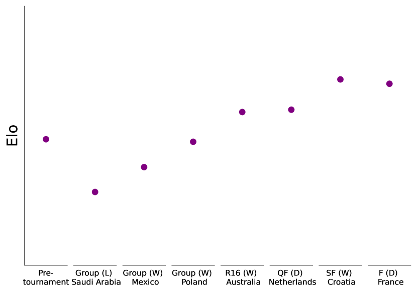
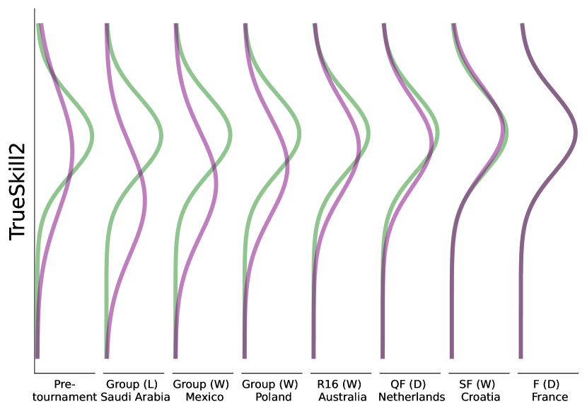
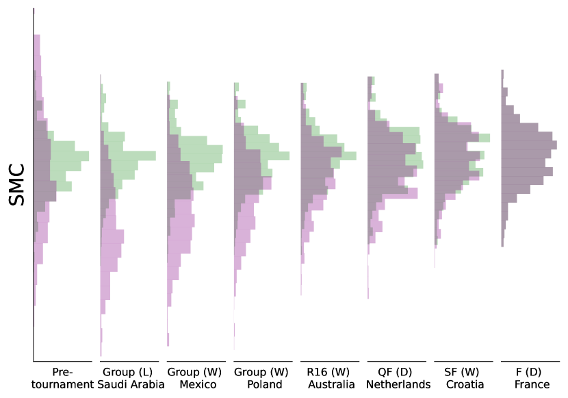
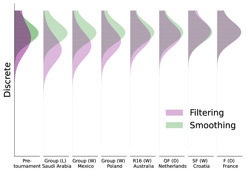
Figure 2: Visualisation of the different (post-match) skill representations for Argentina’s 2023 FIFA World Cup triumph. Each y-axis represents the skill-rating scale for the different approaches (only SMC and TrueSkill2 share the same model and therefore also y-axis scaling).

The first step in any state-space model fitting procedure is to explore the model with some preliminary (perhaps arbitrarily chosen) static parameters. The goal here is not a thorough evaluation of skill ratings, but rather to assess our prior intuitions.

In Fig. 2, we depict Argentina’s 2023 football world cup in terms of the evolution of their skill rating distribution with arbitrarily chosen static parameters (we run on international matches in 2020-2022, with only Argentina’s post-match 2022 world cup ratings displayed). We also take this opportunity to highlight the different approaches to encoding a probability distribution over skill ratings. We first see that Elo stores skill ratings as a point estimate without any uncertainty quantification and that it is a purely forward-based approach without any ability to update skill ratings based on future match results (i.e. smoothing). In contrast, the three model-based SSM approaches encode a (more informative) distribution over skill ratings. In the case of TrueSkill2 (Glicko and Extended Kalman would appear similar and are therefore omitted) a simple location and spread (Gaussian) distribution is used, whereas SMC and the discrete model can encode more complex distributions.

In terms of verifying our intuitions, we can see that Argentine victories increase their skill ratings, draws (against similar sides) have little influence and defeats decrease the ratings. Particularly poignant is Argentina’s defeat to Saudi Arabia (who are a low-ranked side) which in all approaches resulted in a sharp decrease in Argentina’s estimated skill rating.

We can also draw insights from the smoothing distributions. We first note that at the final match in the dataset, the filtering and smoothing distributions match exactly, by definition. We also see that the smoothing distributions show less uncertainty than the filtering distributions; this matches our intuition since smoothing $\mathbf{P}(x_{k}\mid y_{1:K})$ has access to more data than filtering $\mathbf{P}(x_{k}\mid y_{1:k})$. We finally observe that the smoothing distributions are much less reactive to individual results and instead track a smooth trajectory of the team’s skill rating over time.

5.2 Parameter Estimation

Figure 3: Log-likelihood grid and parameter estimation for WTA tennis data. Note that TrueSkill2 and SMC share the same model.

Having verified informally that the algorithms are behaving sensibly, we turn to applying the techniques discussed in Section 3.5 to learn the static parameters from historical data in an offline setting. Our goal is to maximise the log-likelihood $\log\mathbf{P}(y_{1:K}\mid\theta)$.

We initially consider the WTA tennis dataset, which we train on years 2019-2021 and leave 2022 as a test set for later. Draws do not occur in tennis, and therefore we can set $\epsilon=\epsilon_{d}=0$, leaving only two parameters to tune for each (model-based) approach. This two-dimensional optimisation landscape of the log-likelihood can readily be visualised, as in Fig. 3. Indeed, as the static parameter is only two-dimensional the optimisation could be applied using a grid search (as is indeed the most natural option for Elo and Glicko). Furthermore, a filtering sweep provides an estimate of the optimisation objective $\log\mathbf{P}(y_{1:K}\mid\theta)$, and therefore the grid search can be applied directly without running a smoothing routine. For more complex models and datasets, higher dimensional static parameters are inevitable, and a grid search will quickly become prohibitive. We therefore apply iterative expectation-maximisation to the tennis data in Fig. 3 to investigate some of the properties and differences between approaches, indicative of parameter estimation in more complex situations.

For the three approaches considered (we again omit the Extended Kalman approach due to its similarity with TrueSkill2 in all steps beyond filtering), we display 1000 expectation-maximisation iterations starting from three different initialisations.

The TrueSkill2 and SMC approaches share the same model and differ only through their respective Gaussian and particle-based approximations to the skill distributions. The Gaussian approximation induces a significant bias, whereas the particle approximation is asymptotically unbiased, but induces Monte Carlo variance. We can see that the bias from the Gaussian approximation contorts the optimisation landscape for TrueSkill2 relative to SMC, whose landscape is fuzzy due to the stochastic nature of the algorithm. We see that the additional bias from the TrueSkill2 approach results in the EM trajectory evading the global optimum; by contrast, this optimum is successfully identified by both the SMC and discrete approaches, which do not exhibit any systematic bias beyond the factorial approximation.

5.3 Filtering (for online decision-making)

Table 2: Average negative log-likelihood (low is good) for presented models and algorithms across a variety of sports. In each case, the training period was 3 years and the test period was the subsequent year. Note the draw percentages were 0% for tennis, 22% for football and 65% for chess.

Method	Tennis (WTA)		Football (EPL)		Chess
	Train	Test	Train	Test	Train	Test
Elo-Davidson	0.640	0.636	1.000	0.973	0.802	1.001
Glicko	0.640	0.636	-	-	-	-
Extended Kalman	0.640	0.635	0.988	0.965	0.801	0.972
TrueSkill2	0.650	0.668	1.006	0.961	0.802	0.978
SMC	0.640	0.639	0.988	0.962	0.801	0.974
Discrete	0.639	0.636	0.987	0.961	0.801	0.976

Now that we have a principled choice for our static parameters, we can apply the methods to online data. In Table 2, we use static parameters (trained using grid search for Elo and Glicko, and EM for the remaining, model-based approaches). Recall that in the case of sports with draws, Glicko does not provide the normalised outcome predictions required for log-likelihood-based assessment.

For the tennis data, we notice that all models broadly perform quite similarly, with the exception of TrueSkill2; we suspect that this stems from the parameter estimation optimisation issues discussed above. The tennis task without draws represents a simpler binary prediction problem, and it is therefore perhaps not surprising that (with principled parameter estimation) predictive performance saturates. For the more difficult tasks of Football and Chess (where draws do occur), we see that the model-based approaches equipped with uncertainty quantification significantly outperform Elo.

Here we have assessed the accuracy of the approaches in predicting match outcomes, as this is a natural task in the context of online decision-making, and can be useful for a variety of purposes including seeding, scheduling and indeed betting. Predictive distributions can also be used for more sophisticated decision-making such as those based on multiple future matches (competition outcomes, promotion/relegation results, etc.).

5.4 Smoothing (for historical evaluation)

Figure 4: Filtering and smoothing with TrueSkill2 for Tottenham’s EPL matches from 2011-2023. Filtering in purple, smoothing in green (error bars represent one standard deviation) with the other teams’ mean skills in faded grey. Black dashed lines represent a change in Tottenham manager with long-serving ones named.

Smoothing represents an integral subroutine for parameter estimation, though can also be of interest in its own right (Glickman, 1999; Duffield and Singh, 2022). In particular, when analysing the historical evolution of a player’s skill over time, it is more appropriate to consider the smoothing distributions, rather than the filtering distributions which do not update in light of recent match results.

In Fig. 4, we display the historical evolution of Tottenham’s EPL skill rating over time according to (8) and TrueSkill2 inference. When comparing filtering and smoothing, we immediately see that the smoothing distributions are less reactive, and provide a more realistic trajectory of how a team’s underlying skill is expected to evolve over time. Noting that the model permits a certain amount of randomness to occur in each match which can result in surprise results, we observe that the smoothing distributions do a much better job of handling this noise or uncertainty. Fig. 4 only displays the TrueSkill2 method, but of course, similar takeaways hold for all of the aforementioned model-based methods (as is highlighted in Fig. 2).

Historical evaluation of skills can be particularly useful to analyse the impacts of various factors and how they impact the team’s underlying skill level, relative to its competitors. In Fig. 4, we highlight the different managers or head coaches that have served Tottenham during the time period, depicting their competitors’ mean skills in the background. This can be particularly useful in evaluating the ability of the managers and their impact on the team. We observe from the smoothing output that Tottenham’s skill rating was in ascendance under Villas-Boas and early Pochettino, before descending towards the end of the Pochettino era (although perhaps not as sharply as the filtering output would suggest). We note that there are likely many further factors influencing the underlying skill that are not highlighted in Fig. 4, and also that (8) is relatively simple; it may of course be desirable to build a more complex model which can direct account for such additional factors or data.

In practice, one may want to update full smoothing trajectories in an online fashion so that historical evaluation is possible without having to run full $\operatorname{\mathcal{O}}(K)$ backward sweeps. In this setting, a fixed-lag approximation is a natural option (Duffield and Singh, 2022).

6 Discussion

In this work, we have advocated for a model-based approach to the skill rating problem. By taking this perspective, we are able to separate the tasks of modeling and inference. We have detailed a number of basic SSMs which are suitable for tackling the problem. We have also detailed a number of different approximate inference schemes for analysing such models, and discussed their relative strengths and shortcomings. We have conducted a number of case studies on how such methods apply to practical data, highlighting a simple workflow based around the SSM approach, and the different utilities of filtering, smoothing, and parameter estimation in this context.

While we have focused here on relatively simple sporting models, there is of course ample potential to apply the same framework and procedures to more complex models, which we welcome. A simple concrete example would be to model 3-set and 5-set tennis matches with different observation scalings $s_{\text{3-set}}>s_{\text{5-set}}$, to reflect the additional randomness associated with the shorter format. The data and models which we have described have been focused on binary and ternary match outcomes, but the techniques could be easily applied point-by-point or to model margin of victory (Kovalchik, 2020). For example, one could develop a model for cricket skills where the bowler and batter are the two ‘players’ with an asymmetric likelihood based on $\mathcal{Y}=\left\{\text{wicket},\text{extras},0,1,2,3,4,6\right\}$.

Higher-dimensional representations of player skill also represents a natural extension; e.g. home and away strength, surface-dependent strength for tennis players, cricket batter strength v.s. pace/spin, and more. In this setting, the various quantities for a single player may carry significant correlation, suggesting that the factorial approximation ought be applied across player ratings but not within. More broadly, this raises considerations about the scalability of the inference techniques with respect to dimension. These considerations also apply to sports which go beyond pairwise observation models (such as those tackled by TrueSkill (Herbrich et al., 2006; Minka et al., 2018)) although the general joint $\mathsf{Assimilate}$ and $\mathsf{Marginalise}$ framework still applies.

An appealing aspect of our framework is that the user can devote their time to carefully designing their model, and describing their data-generating process in state-space language. Having done this, the general-purpose inference schemes will typically apply directly, enabling the user to easily explore different model and parameter configurations, with the ability to refine the model in an iterative manner (Gelman et al., 2020).

As a result of our specific interests in this problem, we tend to emphasise the role of filtering as a tool for online decision-making, and of smoothing for retrospective evaluation of policies (e.g. assessing coach efficacy, changes in conditions, etc.). For simplicity, we have given a comparatively lightweight treatment of parameter estimation; there are various extensions of our work in this direction which would be worthwhile to examine carefully, e.g. online parameter estimation (Cappé, 2011; Kantas et al., 2015), Bayesian approaches (Andrieu et al., 2010), and beyond.

With regard to practical recommendations, at a coarse resolution we can offer that i) when speed and scalability are of primary interest, Extended Kalman inference offers a good default, whereas ii) when robustness and flexibility are a greater priority, the fHMM model with graph-based inference has many nice properties. We note that the task of evaluating the relative suitability of { Extended Kalman, SMC, HMM, … } approaches is not limited to the skill rating setting, and is relevant across many fields and applications wherein state-space models are fundamental.

Data availability

All data used is freely available online. Tennis data sourced from tennis-data.co.uk.
Football data sourced from football-data.co.uk as well as international football data from github.com/martj42/international_results.
Chess data sourced from github.com/huffyhenry/forecasting-candidates.
Reproducible code can be found at github.com/SamDuffield/abile.

Funding

Sam Power and Lorenzo Rimella were supported by EPSRC grant EP/R018561/1 (Bayes4Health).

Appendix A Algorithm Recursions

We here detail the mathematical recursions underlying the methods in the main text. For brevity, we discuss the recursions in the context of the $\operatorname{\mathcal{O}}(N\cdot K)$ posterior - (1) in the main text. However, any practical implementation should utilise the memory efficient $\operatorname{\mathcal{O}}(N+K)$ match-sparsity posterior - (2) in the main text. Also note that by the factorial approximation, smoothing can be applied independently across players and we therefore omit the player index superscript for the smoothing recursions. A python package with code implementing all of the below can be found at github.com/SamDuffield/abile.

A.1 Elo-Davidson

The Elo-Davidson rating system generalises the original Elo (Elo, 1978) to provide normalised outcome predictions for sports that admit draws (Davidson, 1970). The static parameters are a learning rate $K$, a draw propensity parameter $\kappa$ and a scaling parameter $s$ which we set $s=1$.

A.1.1 Filtering

$$x^{h}_{k}=x_{k-1}^{h}+K\cdot\left(\mathbb{I}[y_{k}=h]+\frac{1}{2}\mathbb{I}[y_{k}=\text{draw}]-g\left(\frac{x_{k-1}^{h}-x_{k-1}^{a}}{s};\kappa\right)\right),$$

$$x^{a}_{k}=x_{k-1}^{a}+K\cdot\left(\mathbb{I}[y_{k}=a]+\frac{1}{2}\mathbb{I}[y_{k}=\text{draw}]-g\left(\frac{x_{k-1}^{a}-x_{k-1}^{h}}{s};\kappa\right)\right),$$

where $g(z;\kappa)=\frac{10^{z}+\kappa/2}{10^{-z}+10^{z}+\kappa}$ and the outcome predictions are given by

$$\mathbf{P}(y_{k}=h) \propto 10^{\frac{x_{k-1}^{h}-x_{k-1}^{a}}{s}}$$

$$\mathbf{P}(y_{k}=a) \propto 10^{\frac{x_{k-1}^{a}-x_{k-1}^{h}}{s}}$$

$$\mathbf{P}(y_{k}=\text{draw}) \propto\kappa.$$

A.1.2 Smoothing and Parameter Estimation

The Elo-Davidson recursions are not explicitly model-based and therefore are not accompanied by smoothing recursions or parameter estimation (beyond optimising the predictive performance objective via grid search on $K$ and $\kappa$, as described in the main paper).

A.2 Glicko

The Glicko rating system (Glickman, 1999) extends Elo to include a time-varying spread variable for each skill rating, i.e. $\operatorname{\mathcal{N}}(x^{i}_{k}\mid\mu^{i}_{k},\sigma^{i\,2}_{k})$.

The static parameters are an initialisation mean $\mu_{0}$ (which we fix as $\mu_{0}=0$), an initialisation spread $\sigma_{0}$, a rate parameter $\tau$, a maximum spread parameter $\sigma_{\text{max}}$ (which we fix to $\sigma_{\text{max}}=\sigma_{0}$) and a scaling parameter $s$ (which we fix as $s=1$).

Glicko does not provide normalised outcome predictions for sports with draws; in the next section, we detail how this can be naturally achieved by adopting a state-space model perspective, and conducting approximate inference by means of the Extended Kalman filter (Ingram, 2021).

A.2.1 Filtering

The Glicko recursions can be thought of as an approximate filtering step (see the main paper for more details on the filtering algorithm)

$$\text{Filter}_{k-1}^{i} =\operatorname{\mathcal{N}}(x_{k-1}^{i}\mid\mu_{k-1}^{i},\sigma_{k-1}^{i\,2}),$$

$$\text{Predict}^{i}_{k} =\operatorname{\mathcal{N}}\left(x_{k}^{i}\mid\mu_{k-1}^{i},\min\left(\sigma_{k-1}^{i\,2}+\tau^{2}\cdot(t_{k}-t_{k-1}),\sigma_{\text{max}}^{2}\right)\right),$$

$$\begin{pmatrix}\text{Filter}_{k}^{h}\\ \text{Filter}_{k}^{a}\end{pmatrix} =\begin{pmatrix}\operatorname{\mathcal{N}}(x_{k}^{i}\mid\mu_{k}^{h},\sigma_{k}^{h\,2})\\ \operatorname{\mathcal{N}}(x_{k}^{i}\mid\mu_{k}^{a},\sigma_{k}^{a\,2})\end{pmatrix}=\mathsf{Assimilate}\left(\begin{pmatrix}\text{Predict}_{k}^{h}\\ \text{Predict}_{k}^{a}\end{pmatrix},y_{k}\right)$$

where the exact form of the $\mathsf{Assimilate}$ equations in the last line, as well as normalised outcome predictions (only for sports without draws), can be found in Section 3.3 of Glickman (1999).

A.2.2 Smoothing and Parameter Estimation

In Glickman (1999), smoothing was conducted by means of the Kalman smoother (which we detail in the next section), and model parameters were specified by numerically minimising the cross-entropy loss between predicted and observed match outcomes.

A.3 Extended Kalman

The Extended Kalman approach allows for the inference procedure of Glicko to be generalised to arbitrary state-space models. Note that for generic SSMs which are either non-linear, non-Gaussian, or both, inference by Extended Kalman methods incurs a systematic bias: the true (non-Gaussian) filtering and smoothing distributions are recursively approximated by Gaussian distributions. This bias is separate to the bias which is incurred throughout by the factorial approximation.

To extend Glicko, we can thus re-use the natural state-space model for pairwise comparisons, (5) in the main text and repeated here

$$m_{0}\left(x_{0}^{i}\right)=\operatorname{\mathcal{N}} \left(x_{0}^{i}\mid\mu_{0},\sigma_{0}^{2}\right),\quad M_{t,t^{\prime}}\left(x^{i}_{t},x^{i}_{t^{\prime}}\right)=\operatorname{\mathcal{N}}\left(x^{i}_{t^{\prime}}\mid x^{i}_{t},\tau^{2}\cdot\left(t^{\prime}-t\right)\right),$$ (8)

$$G_{k}\left(y_{k}\mid x^{h},x^{a}\right) =\begin{cases}\operatorname{\mathbf{sigmoid}}\left(\frac{x^{h}-x^{a}+\epsilon}{s}\right)-\operatorname{\mathbf{sigmoid}}\left(\frac{x^{h}-x^{a}-\epsilon}{s}\right)&\text{if }y_{k}=\text{draw},\\ \operatorname{\mathbf{sigmoid}}\left(\frac{x^{h}-x^{a}-\epsilon}{s}\right)&\text{if }y_{k}=\mathrm{h},\\ 1-\operatorname{\mathbf{sigmoid}}\left(\frac{x^{h}-x^{a}+\epsilon}{s}\right)&\text{if }y_{k}=\mathrm{a}.\end{cases}$$

with static parameters $\theta=(\sigma_{0},\tau,\epsilon)$ and fixed $\mu_{0}=0$ and $s=1$.

A.3.1 Filtering

As with Glicko, we have an analytical $\mathsf{Propagate}$ step

$$\text{Filter}_{k-1}^{i} =\operatorname{\mathcal{N}}(x_{k-1}^{i}\mid\mu_{k-1}^{i},\sigma_{k-1}^{i\,2}),$$

$$\text{Predict}^{i}_{k} =\operatorname{\mathcal{N}}\left(x_{k}^{i}\mid\mu_{k-1}^{i},\sigma_{k-1}^{i\,2}+\tau^{2}\cdot(t_{k}-t_{k-1})\right),$$

noting that we do not synthetically constrain the skill variances as they do.

Due to the non-Gaussian observation model, we cannot conduct the $\mathsf{Assimilate}$ step exactly. Following the Extended Kalman paradigm, we thus proceed by i) computing a second-order Taylor expansion of the log-likelihood $\log G_{k}$ around the predictive means of $x_{k}^{h}$ and $x_{k}^{a}$, ii) converting this into a linear-Gaussian approximate likelihood $\hat{G}_{k}$, i.e.

$$\log\hat{G}_{k}(y\mid x^{h},x^{a}) :=\log G_{k}(y\mid\mu^{h},\mu^{a})$$

$$\quad+(x^{h}-\mu^{h},x^{a}-\mu^{a})\cdot\mathrm{g}_{k}$$

$$\qquad+\frac{1}{2}\cdot(x^{h}-\mu^{h},x^{a}-\mu^{a})\cdot\mathrm{H}_{k}\cdot\begin{pmatrix}x^{h}-\mu^{h}\\ x^{a}-\mu^{a}\end{pmatrix} \in\operatorname{\mathbf{R}},$$

$$\mathrm{g}_{k} =\nabla_{x^{h},x^{a}}\log G_{k}(y\mid x^{h},x^{a})|_{(x^{h},x^{a})=(\mu^{h},\mu^{a})} \in\operatorname{\mathbf{R}}^{2},$$

$$\mathrm{H}_{k} =\nabla_{x^{h},x^{a}}^{2}\log G_{k}(y\mid x^{h},x^{a})|_{(x^{h},x^{a})=(\mu^{h},\mu^{a})} \in\operatorname{\mathbf{R}}^{2\times 2},$$

and then finally iii) exactly assimilating this approximate likelihood, i.e.

$$\text{Filter}^{h,a}_{k}(x^{h}_{k},x^{a}_{k}) \propto\text{Predict}^{h}_{k}(x^{h}_{k})\cdot\text{Predict}^{a}_{k}(x^{a}_{k})\cdot G_{k}(y_{k}\mid x^{h}_{k},x^{a}_{k})$$ (9)

$$\approx\text{Predict}^{h}_{k}(x^{h}_{k})\cdot\text{Predict}^{a}_{k}(x^{a}_{k})\cdot\hat{G}_{k}(y_{k}\mid x^{h}_{k},x^{a}_{k}),$$ (10)

$$\propto\operatorname{\mathcal{N}}\left(\begin{pmatrix}x^{h}_{k}\\ x_{k}^{a}\end{pmatrix}\mid\begin{pmatrix}\mu^{h}_{k}\\ \mu_{k}^{a}\end{pmatrix},\begin{pmatrix}\sigma^{h\,2}_{k}&\rho^{h,a}_{k}\\ \rho^{h,a}_{k}&\sigma^{a\,2}_{k}\end{pmatrix}\right),$$

where the final Gaussian distribution is computed by standard linear-Gaussian conjugacy relations; see Chapter 7 in Särkkä and Svensson (2023).

Note that it would also be possible to make a first-order Taylor approximation if required for higher-dimensional factorial states (i.e. with $\mathrm{H}_{k}=0$). The factorial approximation can then be regained through a $\mathsf{Marginalise}$ step which simply consists of reading off $\mu^{h}_{k},\sigma^{h}_{k}$ and $\mu^{a}_{k},\sigma^{a}_{k}$ and discarding the covariance $\rho^{h,a}_{k}$.

By using the approximate likelihood $\hat{G}_{k}$, this approach can provide normalised outcome predictions, i.e.

$$\hat{\mathbf{P}}(y_{k}\mid y_{1:k-1})=\int\hat{G}_{k}(y_{k}\mid x_{k}^{h},x_{k}^{a})\cdot\text{Predict}^{h}_{k}(x_{k}^{h})\cdot\text{Predict}^{a}_{k}(x^{a}_{k})\;\mathrm{d}x_{k}^{h}\;\mathrm{d}x_{k}^{a}.$$

A.3.2 Smoothing

Given Gaussian filtering approximations and Gaussian dynamics,

$$M_{k,k+1}(x_{k},x_{k+1})=\operatorname{\mathcal{N}}(x_{k+1}\mid x_{k},\tau^{2}\cdot(t_{k+1}-t_{k})),$$

smoothing can carried out analytically using the Kalman smoother; see e.g. Section 7.2 in Chopin and Papaspiliopoulos (2020). That is, given $\text{Filter}_{k}(x_{k})=\operatorname{\mathcal{N}}(x_{k}\mid\mu_{k},\sigma_{k}^{2})$ and $\text{Smooth}_{k+1}(x_{k+1})=\operatorname{\mathcal{N}}(x_{k+1}\mid\mu_{k+1|K},\sigma_{k+1|K}^{2})$, we have the recursions

$$\text{Smooth}_{k|K}(x_{k}) =\operatorname{\mathcal{N}}(x_{k}\mid\mu_{k|K},\sigma_{k|K}^{2}),$$

$$\mathrm{D}_{k} =\sigma_{k}^{2}\cdot(\sigma_{k}^{2}+\tau^{2}\cdot(t_{k+1}-t_{k}))^{-1},$$

$$\mu_{k|K} =\mu_{k}+\mathrm{D}_{k}\cdot(\mu_{k+1|K}-\mu_{k}),$$

$$\sigma^{2}_{k|K} =\sigma^{2}_{k}+\mathrm{D}^{2}_{k}\cdot(\sigma^{2}_{k+1|K}-\sigma^{2}_{k}-\tau^{2}\cdot(t_{k+1}-t_{k})),$$

Additionally, for parameter estimation by expectation-maximisation, it is necessary to compute lag-one autocovariances (i.e. $\mathbf{E}_{\text{Smooth}_{k,k+1|K}}[x_{k}\cdot x_{k+1}]$); these can be recovered from the same output as

$$\mu_{k,k+1|K}:=\mu_{k|K}\cdot\mu_{k+1|K}+\mathrm{D}_{k}\cdot\sigma^{2}_{k+1|K}.$$

The above iterations can then be repeated backwards in time for $k=K-1,\dots,0$, as well as across the $N$ players (independently, according to the factorial approximation).

A.3.3 Parameter Estimation

We can apply an iterative expectation-maximisation algorithm seeking

$$\operatorname*{arg\,max}_{\theta\in\Theta}\mathbf{P}(y_{1:K}\mid\theta).$$

Given a value of the static parameters $\theta_{r}$, we can run our filtering (storing the filtering statistics) and smoothing algorithms to obtain the smoothing statistics

$$\left\{\mu_{0|K}^{i},\sigma_{0|K}^{i},\mu_{0,1|K}^{i},\dots,\mu_{K-1,K|K}^{i},\mu_{K|K}^{i},\sigma_{K|K}^{i}\right\}_{i=1}^{N}.$$

In reality, we only need to obtain $\operatorname{\mathcal{O}}(N+K)$ smoothing statistics (i.e. for players at the matchtimes of matches they were involved in), as described in the section of the main paper on match sparsity. For significant ease of notation, we continue here with the $\operatorname{\mathcal{O}}(N\cdot K)$ description.

We then look to maximise the surrogate objective - (3) in the main text,

$$\mathbf{Q}\left(\theta\mid\hat{\theta}\right):=\int\mathbf{P}\left(x_{0:K}^{\left[N\right]}\mid y_{1:K},\hat{\theta}\right)\cdot\log\mathbf{P}\left(x_{0:K}^{\left[N\right]},y_{1:K}\mid\theta\right)\,\mathrm{d}x_{0:K}^{\left[N\right]},$$ (11)

Using our recursive Gaussian approximation to the smoothing distribution, we can then extract an approximation to the necessary smoothing statistics, yielding a simple approximation to $\mathbf{Q}(\theta\mid\hat{\theta})$. In particular, in the context of our SSM (8) and Gaussian smoothing statistics, we obtain analytically that

$$\hat{\sigma}_{0}^{2} =\frac{1}{N}\sum_{i=1}^{N}\sigma_{0|K}^{i\,2}+\mu_{0|K}^{i\,2},$$

$$\hat{\tau}^{2} =\frac{1}{NK}\sum_{i=1}^{N}\sum_{k=1}^{K}\frac{1}{t_{k}-t_{k-1}}\left[\sigma_{k-1|K}^{i\,2}+\mu_{k-1|K}^{i\,2}-2\mu_{k-1,k|K}^{i}+\sigma_{k|K}^{i\,2}+\mu_{k|K}^{i\,2}\right].$$

For parameters corresponding to the observation density and $\epsilon$ parameter, we are required to evaluate integrals of the form

$$\int\operatorname{\mathcal{N}}(z\mid\mu,\sigma^{2})\cdot\log\left(\operatorname{\mathbf{sigmoid}}(z+\epsilon)-\operatorname{\mathbf{sigmoid}}(z-\epsilon)\right)\,dz,$$

which cannot be evaluated analytically. However, these can be approximated efficiently using e.g. Gauss-Hermite integration, and then $\hat{\epsilon}$ can be found using fast univariate numerical optimisation routines.

We then set $\hat{\theta}\leftarrow(\hat{\sigma}_{0},\hat{\tau},\hat{\epsilon})$ and iterate the above filtering, smoothing, and maximisation steps until convergence.

A.4 TrueSkill2

The TrueSkill2 approach uses the same SSM (8) as the Extended Kalman approach above, but instead using the inverse probit sigmoid function $\operatorname{\mathbf{sigmoid}}_{\text{IP}}(x)=\Phi(x)$ as (inverse) link function.

A.4.1 Filtering

The $\mathsf{Propagate}$ step is again analytically tractable, as in Glicko and the Extended Kalman approach. However, the $\mathsf{Assimilate}$ step is handled differently: instead of Taylor expansion of the log-likelihood, we adopt a moment-matching strategy. In particular, we can use the inverse probit sigmoid and Equation (6) in the main text, repeated here

$$\int\operatorname{\mathcal{N}}(z\mid\mu,\sigma^{2})\Phi(z)\,\mathrm{d}z=\Phi\left(\frac{\mu}{\sqrt{1+\sigma^{2}}}\right).$$ (12)

This allows us to calculate analytically the marginal means and variances of the non-Gaussian joint filtering distribution (10)

$$\mu_{k}^{h}=\mathbf{E}_{\text{Filter}^{h,a}_{k}}\left[x_{k}^{h}\right],\qquad\sigma_{k}^{h\,2}=\mathbf{Var}_{\text{Filter}^{h,a}_{k}}\left[x_{k}^{h}\right]=\mathbf{E}_{\text{Filter}^{h,a}_{k}}\left[\left(x_{k}^{h}-\mu_{k}^{h}\right)^{2}\right],$$

and similarly for $x^{a}_{k}$. That is, the above integrals are analytically tractable. As such, we simply represent our approximate filtering distribution by the Gaussian distribution with this mean and variance, still using the factorial approach to decouple approximations across players. This approach is connected to Assumed Density Filtering (ADF) and Expectation Propagation (EP) methods; see later in this supplement for more details.

The identity in (12) also allows exact computation of the normalised match outcome predictions

$$\mathbf{P}(y_{k}\mid y_{1:k-1})=\int G_{k}(y_{k}\mid x_{k}^{h},x_{k}^{a})\cdot\text{Predict}^{h}_{k}(x_{k}^{h})\cdot\text{Predict}^{a}_{k}(x^{a}_{k})\;\mathrm{d}x_{k}^{h}\;\mathrm{d}x_{k}^{a},$$ (13)

for $y_{k}\in\{\text{draw},\text{home win},\text{away win}\}$.

A.4.2 Smoothing and Parameter Estimation

These steps can be implemented similarly to the Extended Kalman approach above. Note that in Minka et al. (2018), they instead use a gradient step (as opposed to analytical maximisation) within the iterative parameter estimation procedure.

A.5 Sequential Monte Carlo

Sequential Monte Carlo (SMC) (Chopin and Papaspiliopoulos, 2020) takes an importance sampling approach to inference, where a weighted collection of particles is used to approximate otherwise intractable distributions, i.e.

$$p(x)\approx\sum_{j=1}^{J}w^{j}\cdot\delta(x\mid x^{j})$$

for a normalised collection of weights $\sum_{j=1}^{J}w^{j}=1$. SMC is applicable to general SSMs, although in our context of pairwise comparisons, we again focus on (8).

A.5.1 Filtering

For the $\mathsf{Propagate}$ step, we can assume we have a (weighted) particle approximation to the previous filtering distribution

$$\text{Filter}^{i}_{k-1}=\sum_{j=1}^{J}w^{i\,j}_{k-1}\cdot\delta(x_{k-1}^{i}\mid x_{k-1}^{i\,j}).$$

The $\mathsf{Propagate}$ step can then be implemented by simulations, i.e. sampling from the transition kernel $\hat{x}_{k}^{i\,j}\sim M_{k-1,k}\left(x_{k-1}^{i\,j},\cdot\right)$ for $j=1,\dots J$ to give

$$\text{Predict}^{i}_{k|k-1}=\sum_{j=1}^{J}w^{i\,j}_{k-1}\cdot\delta(x_{k}^{i}\mid\hat{x}_{k}^{i\,j}).$$

In certain situations, it can be valuable to instead $\mathsf{Propagate}$ using alternative dynamics, and correct for this discrepancy using importance weighting; we do not pursue this here, but see Doucet et al. (2000) for details.

The $\mathsf{Assimilate}$ step is implemented by i) arbitrarily pairing together particles for the two competing players ii) adjusting the importance weights based on the observation likelihood, iii) normalising and then iv) (optionally) conducting a resampling step. The reweighting (and normalising) gives an approximation to the joint filtering distribution

$$\text{Filter}^{h,a}_{k} =\sum_{j=1}^{J}\hat{w}_{k}^{j}\cdot\delta\left(x^{h}_{k},x^{a}_{k}\mid\hat{x}^{h\,j}_{k},\hat{x}^{a\,j}_{k}\right),$$

$$\hat{w}_{k}^{j} \propto w^{h\,j}_{k-1}\cdot w^{a\,j}_{k-1}\cdot G_{k}\left(y_{k}\mid\hat{x}^{h\,j}_{k},\hat{x}^{a\,j}_{k}\right).$$

This can then be followed by a resampling step, giving

$$\text{Filter}^{h,a}_{k} \approx\sum_{j=1}^{J}w_{k}^{j}\cdot\delta\left(x^{h}_{k},x^{a}_{k}\mid x^{h\,j}_{k},x^{a\,j}_{k}\right),$$

where $w_{k}^{j}\equiv\frac{1}{J}$ and $x^{h}_{k},x^{a}_{k}\sim\text{Filter}^{h,a}_{k}$ if resampling is applied; otherwise $w_{k}^{j}=\hat{w}_{k}^{j}$ and $x^{h}_{k},x^{a}_{k}=\hat{x}^{h}_{k},\hat{x}^{a}_{k}$. The resampling operation ensures that low-probability particles are not carried through to the next iteration and stabilises the weights, thereby ensuring a suitably diverse particle approximation and good long-time stability properties. The simplest resampling approach is to apply multinomial resampling at every $\mathsf{Assimilate}$ step (as used in our experiments); more sophisticated resampling methods including stratified resampling and adaptive approaches are also common in practice (Douc and Cappé, 2005).

The $\mathsf{Marginalise}$ step can then be applied be simply unpairing the joint $\text{Filter}^{h,a}_{k}$ in line with the factorial approximation, i.e.

$$\text{Filter}^{h}_{k}=\sum_{j=1}^{J}w_{k}^{j}\cdot\delta\left(x^{h}_{k}\mid x^{h\,j}_{k}\right),\qquad\text{Filter}^{a}_{k}=\sum_{j=1}^{J}w_{k}^{j}\cdot\delta\left(x^{a}_{k}\mid x^{a\,j}_{k}\right).$$

Note that the $\mathsf{Assimilate}$ step could be made more robust by considering all possible $J^{2}$ pairings (as opposed to the arbitrary $J$ pairings of skills) between the two players.

Normalised match outcome predictions can be obtained by direct particle approximation to (13).

A.5.2 Smoothing

Smoothing can be applied by use of backward simulation (Godsill et al., 2004), which re-uses the filtering particle approximations to provide an approximation to full smoothing trajectories $\text{Smooth}_{0:K|K}\approx\frac{1}{J}\sum_{j=1}^{J}\delta\left(x_{0:K}\mid x^{j}_{0:K|K}\right)$. Assuming that we have an unweighted particle approximation to $\text{Smooth}_{k+1|K}\approx\frac{1}{J}\sum_{j=1}^{J}\delta\left(x_{k+1}\mid x^{j}_{k+1|K}\right)$ and a weighted particle approximation to $\text{Filter}_{k}\approx\sum_{j=1}^{J}w_{k}^{j}\cdot\delta\left(x_{k}\mid x^{j}_{k}\right)$, we can then sample to form an approximation to $\text{Smooth}_{k,k+1|K}$

$$x_{k|K}^{j} \sim\sum_{j^{\prime}=1}^{J}w_{k}^{j^{\prime}\leftarrow j}\cdot\delta\left(x_{k}\mid x^{j^{\prime}}_{k}\right),$$

$$\text{where}\quad w_{k}^{j^{\prime}\leftarrow j} \propto w_{k}^{j^{\prime}}\cdot M_{k,k+1}\left(x^{j^{\prime}}_{k},x^{j}_{k+1|K}\right).$$

This procedure can then be iterated for $k=K-1,\dots,0$ to provide an approximation to $\text{Smooth}_{0:K|K}$. The standard backward simulation detailed above has complexity $\operatorname{\mathcal{O}}(J^{2})$; note however that methods based on rejection sampling (Douc et al., 2011) and MCMC (Dau and Chopin, 2023) have been developed in order to reduce the complexity to $\operatorname{\mathcal{O}}(J)$.

A.5.3 Parameter Estimation

For a particle approximation to $\text{Smooth}_{0:K|K}\approx\frac{1}{J}\sum_{j=1}^{J}\delta\left(x_{0:K}\mid x^{j}_{0:K|K}\right)$, maximisation of the surrogate objective (11) is tractable for $\sigma_{0}$ and $\tau$ (as in the Gaussian approximation case). This yields the updates

$$\hat{\sigma}_{0}^{2} =\frac{1}{NJ}\sum_{i=1}^{N}\sum_{j=1}^{J}x_{0|K}^{i\,j\,2},$$

$$\hat{\tau}^{2} =\frac{1}{NTJ}\sum_{i=1}^{N}\sum_{k=1}^{K}\sum_{j=1}^{J}\frac{1}{t_{k}-t_{k-1}}\left(x^{i\,j}_{k|K}-x^{i\,j}_{k-1|K}\right)^{2}.$$

Similarly to before, we update $\epsilon$ by univariate numerical maximisation methods.

A.6 Factorial Hidden Markov Model

In an HMM approach, the player skill ratings take values in a discrete set $\mathcal{X}=\left[S\right]$ for some $S\in\mathbf{N}$, which leads to a closed form for the operations $\left\{\mathsf{Propagate},\mathsf{Assimilate},\mathsf{Bridge}\right\}$. However, as mentioned in the main text, the cost of these operations might be exponentially large in the dimension of the state space, and so computationally unfeasible. We can then adopt the decoupling approximation and exploit the factorial structure in the dynamics of the fHMM (Rimella and Whiteley, 2022). For the decoupling approximation, the only thing we have to define is the form of $\left\{\mathsf{Propagate},\mathsf{Assimilate},\mathsf{Bridge},\mathsf{Marginalise}\right\}$, which will then lead to the recursive algorithm. Note also that the flexibility of the fHMM means that we are not limited to specific choices of the transition kernel $M_{k-1,k}$ and emission distribution $G_{k}$, and so we keep them general in the following sections. That is, we assume only that $M_{k-1,k}$ is an $S\times S$ stochastic matrix and that for any $y\in\mathcal{Y}$, $G_{k}(y\mid\cdot,\cdot)$ is an $S\times S$ matrix.

A.6.1 Assembling the kernel

Before starting, it is important to briefly explain why explicitly assembling the transition kernel $M_{t,t^{\prime}}$ is inadvisable unless strictly necessary. Recall that we define the dynamics in terms of the generator matrix $Q_{S}$, and as such $M_{t,t^{\prime}}$ is expressible as matrix exponential, i.e.

$$M_{t,t^{\prime}}=\exp\left(\tau_{d}\cdot(t^{\prime}-t)\cdot Q_{S}\right).$$

In principle, computing this matrix for each $t,t^{\prime}$ incurs a cost of $\operatorname{\mathcal{O}}(S^{3})$. However, this is wasteful: for filtering purposes, we only need to access $M_{t,t^{\prime}}$ through its action on probability vectors, which costs only $\operatorname{\mathcal{O}}(S^{2})$ once the matrix is available. We will thus try to describe these matrices in a way which enables these rapid computations.

In particular, when possible, it is worthwhile to instead pre-compute a diagonalisation of $Q_{S}$, i.e. identify an invertible matrix $\Psi_{S}$ and diagonal matrix $\Lambda_{S}$ such that

$$Q_{S}=\Psi_{S}^{-1}\cdot\Lambda_{S}\cdot\Psi_{S},$$

noting that for self-adjoint $Q_{S}$, $\Psi_{S}$ will be orthogonal. For the example considered in the main text, we detail this decomposition in Appendix B.

Given such a decomposition, the transition kernel then takes the form

$$M_{t,t^{\prime}} =\Psi_{S}^{-1}\cdot\exp\left(-\tau_{d}\cdot(t^{\prime}-t)\cdot\Lambda_{S}\right)\cdot\Psi_{S}.$$

We can thus compute expressions like $\pi M_{t,t^{\prime}}$ by

$$\pi_{0} =\pi$$ (14)

$$\pi_{1} =\pi_{0}\cdot\Psi_{S}^{-1}$$ (15)

$$\pi_{2} =\pi_{1}\cdot\exp\left(-\tau_{d}\cdot(t^{\prime}-t)\cdot\Lambda_{S}\right)$$ (16)

$$\pi_{3} =\pi_{2}\cdot\Psi_{S}.$$ (17)

The first and third steps are standard matrix-vector products, costing $\operatorname{\mathcal{O}}(S^{2})$, whereas the second step is a diagonal matrix-vector product, costing only $\operatorname{\mathcal{O}}(S)$. We thus see that a judicious one-off matrix decomposition costing $\operatorname{\mathcal{O}}(S^{3})$ allows us to reduce the cost of all future filtering updates to $\operatorname{\mathcal{O}}(S^{2})$.

Note that in this framework assembling $M_{t,t^{\prime}}$ has a computational cost of $\operatorname{\mathcal{O}}(S^{3})$, while vector matrix multiplication with $M_{t,t^{\prime}}$ remains $\operatorname{\mathcal{O}}(S^{2})$.

In the next sections, we will see that filtering is not an issue as it requires vector-matrix multiplication with the kernel, while vanilla smoothing requires elementwise products with the transition kernel and so does not simplify in a straightforward vector-matrix operation. However, we can modify the smoothing recursions to require vector-matrix operations only.

A.6.2 Filtering

Here we explain the general step $k$ in the filtering recursion in the context of the $\operatorname{\mathcal{O}}(N\cdot K)$ representation. This requires performing a $\mathsf{Propagate}$ step and $\mathsf{Assimilate}$ on players $h,a$.

The $\mathsf{Propagate}$ step at time $k$ consists of propagating the filtering distribution through the transition kernel. In finite state spaces, this is a straightforward matrix-vector operation. In particular, for $i\in[N]$, we do

$$\mathrm{Predict}_{k\mid k-1}^{i} =\mathsf{Propagate}\left(\mathrm{Filter}_{k-1}^{i};M_{{k-1},k}\right)$$

$$=\mathrm{Filter}_{k-1}^{i}\cdot M_{{k-1},k},$$

noting that we represent probability vectors as row vectors.

$\mathsf{Assimilate}$ requires a joint update on both players $h$ and $a$, and so outputs the joint distribution $\mathrm{Filter}^{h,a}_{k}$ in the form of a ${S\times S}$ matrix with elements summing to $1$. Precisely, given the current match outcome $y_{k}$, the joint filter takes the form

$$\mathrm{Filter}^{h,a}_{k} =\mathsf{Assimilate}\left(\left(\begin{array}[]{c}\mathrm{Predict}^{h}_{k|k-1}\\ \mathrm{Predict}^{a}_{k|k-1}\end{array}\right);G_{k}\right)$$

$$\propto\left(\left(\mathrm{Predict}_{k\mid k-1}^{h}\right)^{\mathrm{T}}\cdot\mathrm{Predict}_{k\mid k-1}^{a}\right)\odot G_{k}(y_{k}\mid\cdot,\cdot),$$

where the operation $\odot$ denotes elementwise product between matrices. Observe that on the left hand side of $\odot$ we have the joint prediction on the skill level of $h$ and $a$, while on the right hand side we have the emission score from the match result. It is also important to notice that we have a proportional sign, meaning that we need to normalize our computation to a joint distribution on ${S\times S}$.

Noting that our $\mathsf{Propagate}$ operator acts on player-wise filtering distribution, it remains to convert $\mathrm{Filter}^{h,a}_{k}$ into a product of marginals. To do so, we simply compute the marginals along $h$ and $a$, i.e. sum over the columns and sum over the rows

$$\left(\begin{array}[]{c}\mathrm{Filter}^{h}_{k}\\ \mathrm{Filter}^{a}_{k}\end{array}\right)=\left(\begin{array}[]{c}\mathsf{Marginalise}\left(\mathrm{Filter}^{h,a}_{k};h\right)\\ \mathsf{Marginalise}\left(\mathrm{Filter}^{h,a}_{k};a\right)\end{array}\right)=\left(\begin{array}[]{c}\left(\mathrm{Filter}^{h,a}_{k}\cdot 1_{S}^{\top}\right)^{\top}\\ 1_{S}\cdot\mathrm{Filter}^{h,a}_{k}\end{array}\right),$$

where $1_{S}$ is the $S$-dimensional row vector of ones.

Overall, the computational cost of a filtering step is $\operatorname{\mathcal{O}}(S^{2})$ per each player, as it requires linear algebra operation on $S$-dimensional vectors and $S\times S$-dimensional matrices. Note that the we are omitting the $\operatorname{\mathcal{O}}(S^{3})$ cost of the initial matrix decomposition (as it has a complexity independent of both $N$ and $K$), as well as the $\operatorname{\mathcal{O}}(S^{3})$ cost of assembling the matrices $M_{t,t^{\prime}}$, which (as described above) is not necessary for either filtering or prediction.

Normalised match outcome predictions can be obtained by evaluating the integral (13) exactly via linear algebra.

A.6.3 Smoothing

This section details a general step of the smoothing algorithm. Recall that by our decoupling approximation, smoothing can carried out independently across players. As such, we temporarily drop the player indices from our notation.

To run the $k$th backward step of the smoothing algorithm, we require the row vectors $\mathrm{Filter}_{k}$ and $\mathrm{Smooth}_{k+1\mid K}$, representing the filtering distribution of the skills of a player at time $k$, and the smoothing distribution of the skills of the same player at time $k+1$. For a general smoothing step we need the operations $\left\{\mathsf{Bridge},\mathsf{Marginalise}\right\}$, where $\mathsf{Bridge}$ generates a joint distribution on the skills of the players on time steps $k,k+1$ and $\mathsf{Marginalise}$ converts this joint distribution in a marginal over earlier time step $k$. As for the filtering step, all operations rely only on basic linear algebra routines:

$$\begin{split}\mathrm{Smooth}_{k,k+1\mid K}&=\mathsf{Bridge}\left(\mathrm{Filter}_{k},\mathrm{Smooth}_{k+1\mid K};M_{k,{k+1}}\right)\\ &=\left[\mathrm{Filter}_{k}^{\top}\cdot\left(\mathrm{Smooth}_{k+1\mid K}\fatbslash\mathrm{Predict}_{k+1\mid k}\right)\right]\odot M_{k,k+1}\\ \mathrm{Smooth}_{k\mid K}&=\mathsf{Marginalise}\left(\mathrm{Smooth}_{k,k+1\mid K};k\right)=\left(\mathrm{Smooth}_{k,k+1\mid K}\cdot 1_{S}^{\top}\right)^{\top},\end{split}$$

where $\fatbslash$ denotes elementwise division.

Given access to the transition matrix $M_{k,k+1}$, one sees that the smoothing step has a computational cost of $\operatorname{\mathcal{O}}(S^{2})$; it thus remains to assemble this matrix, at a cost of $\operatorname{\mathcal{O}}(S^{3})$.

However, there is an alternative formulation of the smoothing step which avoids assembling the joint distribution by merging the $\mathsf{Marginalise}$ and $\mathsf{Bridge}$ steps:

$$\begin{split}\mathrm{Predict}_{k+1\mid k}&=\mathrm{Filter}_{k}\cdot M_{k,k+1},\\ \mathrm{Smooth}_{k\mid K}&=\mathrm{Filter}_{k}\odot\left[\left(\mathrm{Smooth}_{k+1\mid K}\fatbslash\mathrm{Predict}_{k+1\mid k}\right)\cdot M_{k,k+1}^{\top}\right].\end{split}$$

The derivation comes from carefully reordering the operations in such a way that we perform the marginalisation on $k+1$ first, indeed

$$\begin{split}&\left[\mathrm{Filter}_{k}^{\top}\cdot\left(\mathrm{Smooth}_{k+1\mid K}\fatbslash\mathrm{Predict}_{k+1\mid k}\right)\right]\odot M_{k,k+1}\\ &=\left(\mathrm{Filter}_{k}^{\top}\cdot 1_{S}\right)\odot M_{k,k+1}\odot\left[1_{S}^{\top}\cdot\left(\mathrm{Smooth}_{k+1\mid K}\fatbslash\mathrm{Predict}_{k+1\mid k}\right)\right]\end{split}$$ (18)

and

$$\begin{split}&\left\{\left(\mathrm{Filter}_{k}^{\top}\cdot 1_{S}\right)\odot M_{k,k+1}\odot\left[1_{S}^{\top}\cdot\left(\mathrm{Smooth}_{k+1\mid K}\fatbslash\mathrm{Predict}_{k+1\mid k}\right)\right]\right\}\cdot 1_{S}^{\top}\\ &=\mathrm{Filter}_{k}^{\top}\odot\left(\left\{M_{k,k+1}\odot\left[1_{S}^{\top}\cdot\left(\mathrm{Smooth}_{k+1\mid K}\fatbslash\mathrm{Predict}_{k+1\mid k}\right)\right]\right\}\cdot 1_{S}^{\top}\right)\\ &=\mathrm{Filter}_{k}^{\top}\odot\left[M_{k,k+1}\cdot\left(\mathrm{Smooth}_{k+1\mid K}\fatbslash\mathrm{Predict}_{k+1\mid k}\right)^{\top}\right]\end{split}$$ (19)

where the first equality follows from noting that $\left(\mathrm{Filter}_{k}^{\top}\cdot 1_{S}\right)$ is constant within rows, and the second from noting that $1_{S}^{\top}\cdot\left(\mathrm{Smooth}_{k+1\mid K}\fatbslash\mathrm{Predict}_{k+1\mid k}\right)$ is constant within columns. This alternative perspective on the smoothing step is crucial, as by avoiding the assembly of the transition kernel, we are able to control the cost of smoothing iterations at the much lower $\operatorname{\mathcal{O}}(S^{2})$.

A.6.4 Parameter Estimation

In this section we make explicit the dependence of the model on the parameters $\theta$. In our setting, the parameters are also decoupled, with respect to their impact initial distribution, transition kernel and emission distribution. That is, with $\theta=(\sigma_{d},\tau_{d},\epsilon_{d})$, only $\sigma_{d}$ influences the initial distribution, only $\tau_{d}$ the transition kernel, and only $\epsilon_{d}$ the emission distribution, with .

Towards implementing the EM algorithm, we recall the definition of $\mathbf{Q}(\theta|\hat{\theta})$ and simply substitute the true smoothing distribution with our decoupled approximation. The resulting $\mathbf{Q}$ function which we seek to maximise may then be expressed as

$$\mathbf{Q}(\theta|\hat{\theta}) =\int\mathbf{P}\left(x_{0:K}^{[N]}\mid{y}_{1:K},\hat{\theta}\right)\cdot\log\mathbf{P}\left(x_{0:K}^{[N]},{y}_{1:K}\mid{\theta}\right)\,\mathrm{d}x_{0:K}^{[N]}$$

$$=\mathbf{Q}_{1}(\sigma_{d}|\hat{\theta})+\mathbf{Q}_{2}(\tau_{d}|\hat{\theta})+\mathbf{Q}_{3}(\epsilon_{d}|\hat{\theta}),$$

where

$$\mathbf{Q}_{1}(\sigma_{d}|\hat{\theta}) =\sum_{i\in[N]}\int\mathbf{P}\left(x_{0}^{i}\mid{y}_{1:K},\hat{\theta}\right)\cdot\log m_{0}\left({x}_{0}^{i}\mid\sigma_{d}\right)\,\mathrm{d}x_{0}^{i}$$

$$\mathbf{Q}_{2}(\tau_{d}|\hat{\theta}) =\sum_{i\in[N]}\sum_{k=1}^{K}\int\mathbf{P}\left(x_{k-1}^{i},x_{k}^{i}\mid{y}_{1:K},\hat{\theta}\right)\cdot\log M_{k-1,k}\left(x^{i}_{k-1},x^{i}_{k}\mid\tau_{d}\right)\,\mathrm{d}x^{i}_{k-1}\,\mathrm{d}x^{i}_{k}$$

$$\mathbf{Q}_{3}(\epsilon_{d}|\hat{\theta}) =\sum_{k=1}^{K}\int\mathbf{P}\left(x_{k}^{h(k)},x_{k}^{a(k)}\mid{y}_{1:K},\hat{\theta}\right)\cdot\log G_{k}\left(y_{k}\mid x_{k}^{h(k)},x_{k}^{a(k)}\mid\epsilon_{d}\right)\,\mathrm{d}{x}_{k}^{h(k)}\mathrm{d}{x}_{k}^{a(k)}.$$

We can then minimise each of these objective functions separately.

One practical difficulty is that in order to construct $\mathbf{Q}_{2}$, we require access to the two-step joint smoothing distributions, i.e. $\mathrm{Smooth}_{k-1,k\mid K}$. Assembling this distribution incurs an undesirable cost of $\operatorname{\mathcal{O}}(S^{3})$, which we prefer to avoid. As such, we proceed with the following hybrid method:

1. Compute the single-step smoothing laws using the $\operatorname{\mathcal{O}}(S^{2})$ algorithm.

2. Use the single-step smoothing laws to update the parameters of the initial distribution and emission distribution in closed form.

3. Compute the gradient of $\mathbf{Q}_{2}(\tau_{d}\mid\hat{\theta})$ with respect to $\tau_{d}$, and

4. Update $\tau_{d}$ by applying a gradient step.

We now detail how this gradient is computed. Focusing on $\mathbf{Q}_{2}$, we expand the joint smoothing distribution to write

$$\begin{split}\frac{\partial\mathbf{Q}_{2}\left(\tau_{d}|\hat{\theta}\right)}{\partial\tau_{d}}&=\sum_{i\in\left[N\right]}\sum_{k=1}^{K}\sum_{a,b\in\left[S\right]}\frac{\frac{\partial}{\partial\tau_{d}}M_{k-1,k}\left(a,b\mid\tau_{d}\right)}{M_{k-1,k}\left(a,b\mid\tau_{d}\right)}\cdot\mathrm{Smooth}_{k-1,k\mid K}^{i}\left(a,b\mid\hat{\theta}\right)\\ &=\sum_{i\in\left[N\right]}\sum_{k=1}^{K}\sum_{a,b\in\left[S\right]}\frac{\frac{\partial}{\partial\tau_{d}}M_{k-1,k}\left(a,b\mid\tau_{d}\right)}{M_{k-1,k}\left(a,b\mid\tau_{d}\right)}\\ &\cdot\frac{\mathrm{Filter}_{k-1}^{i}\left(a\mid\hat{\theta}\right)\cdot\mathrm{Smooth}_{k\mid K}^{i}\left(b\mid\hat{\theta}\right)\cdot M_{k-1,k}\left(a,b\mid\hat{\tau}_{d}\right)}{\sum_{\bar{a},\bar{b}\in\left[S\right]}\mathrm{Filter}_{k-1}^{i}\left(\bar{a}\mid\hat{\theta}\right)\cdot\mathrm{Smooth}_{k\mid K}^{i}\left(\bar{b}\mid\hat{\theta}\right)\cdot M_{k-1,k}\left(\bar{a},\bar{b}\mid\hat{\tau}_{d}\right)}.\end{split}$$

This expression can be simplified further if we consider its value at $\tau_{d}=\hat{\tau}_{d}$. We obtain

$$\begin{split}&\frac{\partial\mathbf{Q}_{2}\left(\tau_{d}|\hat{\theta}\right)}{\partial\tau_{d}}=\sum_{i\in\left[N\right]}\sum_{k=1}^{K}\sum_{a,b\in\left[S\right]}\left[\frac{\partial}{\partial\tau_{d}}M_{k-1,k}\left(a,b\mid\hat{\tau}_{d}\right)\right]\\ &\cdot\frac{\mathrm{Filter}_{k-1}^{i}\left(a\mid\hat{\theta}\right)\cdot\mathrm{Smooth}_{k\mid K}^{i}\left(b\mid\hat{\theta}\right)}{\sum_{\bar{a},\bar{b}\in\left[S\right]}\mathrm{Filter}_{k-1}^{i}\left(\bar{a}\mid\hat{\theta}\right)\cdot\mathrm{Smooth}_{k\mid K}^{i}\left(\bar{b}\mid\hat{\theta}\right)\cdot M_{k-1,k}\left(\bar{a},\bar{b}\mid\hat{\tau}_{d}\right)}.\end{split}$$ (20)

Now, suppose that $Q_{S}=\Psi_{S}^{-1}\cdot\Lambda_{S}\cdot\Psi_{S}$, and that $\tau_{d}=\tau_{d}$ is a rate parameter, i.e.

$$M_{t,t^{\prime}}\left(\cdot\mid\tau_{d}\right)=\exp\left(\tau_{d}\cdot\left(t^{\prime}-t\right)\cdot Q_{S}\right).$$

It then holds that

$$\frac{\partial}{\partial\tau_{d}}M_{k-1,k}\left(a,b\mid\hat{\tau}_{d}\right) =\frac{\partial}{\partial\tau_{d}}\exp\left(\tau_{d}\cdot\left(t_{k}-t_{k-1}\right)\cdot Q_{S}\right)$$

$$=\exp\left(\tau_{d}\cdot\left(t_{k}-t_{k-1}\right)\cdot Q_{S}\right)\cdot\left(t_{k}-t_{k-1}\right)\cdot Q_{S}$$

$$=\Psi_{S}^{-1}\cdot\left[\left(t_{k}-t_{k-1}\right)\cdot\Lambda_{S}\cdot\exp\left(\tau_{d}\cdot\left(t_{k}-t_{k-1}\right)\Lambda_{S}\right)\right]\cdot\Psi_{S},$$

where the term in brackets is again a diagonal matrix. The gradient can then be assembled as follows

$$\mathrm{F}_{k-1}^{i} \leftarrow\left(\mathrm{Filter}_{k-1}^{i}\right)\cdot\Psi_{S}^{-1}$$

$$\mathrm{S}_{k}^{i} \leftarrow\left(\mathrm{Smooth}_{k\mid K}^{i}\right)\cdot\Psi_{S}^{-1}$$

$$\tilde{\Lambda}_{S}^{k} \leftarrow\left(t_{k}-t_{k-1}\right)\cdot\Lambda_{S}\cdot\exp\left(\tau_{d}\cdot\left(t_{k}-t_{k-1}\right)\Lambda_{S}\right)$$

$$\mathrm{N}_{k-1,k}^{i} =\mathrm{F}_{k-1}^{i}\cdot\tilde{\Lambda}_{S}^{k}\cdot\left(\mathrm{S}_{k}^{i}\right)^{\top}$$

$$\mathrm{D}_{k-1,k}^{i} =\mathrm{F}_{k-1}^{i}\cdot\Lambda_{S}\cdot\left(\mathrm{S}_{k}^{i}\right)^{\top}$$

$$\frac{\partial\mathbf{Q}_{2}\left(\tau_{d}|\hat{\theta}\right)}{\partial\tau_{d}} =\sum_{i\in\left[N\right]}\sum_{k=1}^{K}\frac{\mathrm{N}_{k-1,k}^{i}}{\mathrm{D}_{k-1,k}^{i}},$$

wherein the first two terms can be constructed in time $\operatorname{\mathcal{O}}(S^{2})$, and the subsequent three terms in time $\operatorname{\mathcal{O}}(S)$. For generator matrices with more elaborate dependence on parameters, we expect that more specialised routines may be necessary. This is largely a by-product of the non-commutativity of matrices, which complicates the computation of expressions like $\nabla_{\theta}\exp\left(Q\left(\theta\right)\right)$.

Appendix B Continuous time Random Walk for Finite State Spaces

For the fHMM model used in Section 4.5 of the main text, we take our dynamics to be the Continuous-Time Reflected Random Walk on $\left[S\right]$, which we construct as follows. Let $P_{S}$ denote the transition matrix for the Discrete-Time Reflected Random Walk on $\left[S\right]$, i.e.

$$\left(P_{S}\right)_{i,j}=\begin{cases}\frac{1}{2}&1<i,j<S,\left|i-j\right|=1\\ \frac{1}{2}&\left(i,j\right)\in\left\{\left(1,2\right),\left(S,S-1\right)\right\}\\ 0&\text{otherwise},\end{cases}$$

noting that this process admits the normalised uniform measure on $\left[S\right]$ as its unique invariant probability measure, and is even reversible with respect to it. As such, we know that $P_{S}$ admits an eigenvalue decomposition of the form $P_{S}=\Psi_{S}^{\top}\cdot\tilde{\Lambda}_{S}\cdot\Psi_{S}$, where $\Psi_{S}$ is orthogonal, and $\tilde{\Lambda}_{S}$ is diagonal. In fact, $\left(\Psi_{S},\tilde{\Lambda}_{S}\right)$ can be computed analytically as

$$\left(\tilde{\Lambda}_{S}\right)_{i,i} =\cos\left(\frac{2\cdot\pi\cdot\left(i-1\right)}{S}\right)$$

$$\left(\Psi_{S}\right)_{i,j} =\begin{cases}S^{-1/2}&i=1\\ \left(S/2\right)^{-1/2}\cdot\cos\left(\frac{\pi\cdot\left(i-1\right)\cdot\left(2\cdot j-1\right)}{S}\right)&1<i\leqslant S.\end{cases}$$

We now define the continuous-time process as the Poissonisation of the discrete-time process with transition matrix $P_{S}$, whose generator matrix is obtained as $Q_{S}=P_{S}-I_{S}$. One then sees that $Q_{S}$ admits the eigenvalue decomposition $Q_{S}=\Psi_{S}^{\top}\cdot\Lambda_{S}\cdot\Psi_{S}$, with $\Lambda_{S}=\tilde{\Lambda}_{S}-I_{S}$, which is again fully explicit.

Appendix C Expectation-Propagation and Assumed Density Filtering

Assumed Density Filtering (ADF) is a general tool for approximate filtering; see Chapter 1 of Minka (2001b) for some overview and many references. In a particularly narrow form, ADF applies to state-space models for which i) there exists a parametric family $\mathcal{F}$ of distributions which is preserved by the dynamics, but ii) the observation model is not necessarily conjugate to this family. Approximating the filtering and predictive distributions by elements of $\mathcal{F}$, ADF then proceeds by implementing the $\mathsf{Propagate}$ step exactly, and approximating the $\mathsf{Assimilate}$ step. When the parametric family is an exponential family of distributions, this approximation is typically implemented by a moment-matching step based on the sufficient statistics of the exponential family, i.e.

$$\mathrm{ExactFilter} =\mathsf{ExactAssimilate}\left(\mathrm{Predict},G\right)$$

$$\mathrm{Filter} =\mathsf{MomentMatch}_{\mathcal{F}}\left(\mathrm{ExactFilter}\right),$$

so that one might write $\mathsf{Assimilate}=\mathsf{MomentMatch}_{\mathcal{F}}\circ\mathsf{ExactAssimilate}$.

A broader interpretation of ADF would allow for non-conjugate dynamics which are then projected back onto the parametric family, implemented by e.g. $\mathsf{Propagate}=\mathsf{MomentMatch}_{\mathcal{F}}\circ\mathsf{ExactPropagate}$. In general, the feasibility of ADF for any specific model is constrained only by the availability of a suitable parametric family of distributions, and the user’s ability to compute the relevant measure projections (by e.g. computing moments).

Expectation Propagation (EP) is an extension of ADF to graphical models which do not necessarily admit a temporal (or even tree-based) structure; see e.g. Minka (2001a).

For the specific case of inference in the dynamic Bradley-Terry model, ADF-type strategies offer an alternative to the mode-centred linearisation strategy of the Extended Kalman filter. This is potentially appealing, as such linearisation strategies are observed to be problematic for skewed likelihoods, which are commonplace in models with binary observations, as we have. In such settings, moment-matching approaches like ADF are observed to have improved robustness properties. See Kuss et al. (2005) for extensive discussion.

References

- Andrieu et al. (2010) Andrieu, C., A. Doucet, and R. Holenstein (2010). Particle Markov chain Monte Carlo methods. Journal of the Royal Statistical Society Series B: Statistical Methodology 72(3), 269–342.
- Bradley and Terry (1952) Bradley, R. A. and M. E. Terry (1952). Rank Analysis of Incomplete Block Designs: I. The Method of Paired Comparisons. Biometrika 39(3/4), 324–345.
- Cappé (2011) Cappé, O. (2011). Online EM algorithm for hidden Markov models. Journal of Computational and Graphical Statistics 20(3), 728–749.
- Chopin and Papaspiliopoulos (2020) Chopin, N. and O. Papaspiliopoulos (2020). Introduction to Sequential Monte Carlo. Springer International Publishing.
- Dangauthier et al. (2008) Dangauthier, P., R. Herbrich, T. Minka, and T. Graepel (2008). Trueskill Through Time: Revisiting the History of Chess. In J. Platt, D. Koller, Y. Singer, and S. Roweis (Eds.), Advances in Neural Information Processing Systems, Volume 20. Curran Associates, Inc.
- Dau and Chopin (2023) Dau, H.-D. and N. Chopin (2023). On backward smoothing algorithms.
- Davidson (1970) Davidson, R. R. (1970). On Extending the Bradley-Terry model to Accommodate Ties in Paired Comparison Experiments. Journal of the American Statistical Association 65(329), 317–328.
- Del Moral et al. (2010) Del Moral, P., A. Doucet, and S. Singh (2010). Forward smoothing using sequential monte carlo.
- Douc and Cappé (2005) Douc, R. and O. Cappé (2005). Comparison of resampling schemes for particle filtering. In ISPA 2005. Proceedings of the 4th International Symposium on Image and Signal Processing and Analysis, 2005., pp. 64–69. IEEE.
- Douc et al. (2011) Douc, R., A. Garivier, E. Moulines, and J. Olsson (2011). Sequential Monte Carlo smoothing for general state space hidden Markov models. The Annals of Applied Probability 21(6), 2109 – 2145.
- Doucet et al. (2000) Doucet, A., S. Godsill, and C. Andrieu (2000). On sequential Monte Carlo sampling methods for Bayesian filtering. Statistics and computing 10, 197–208.
- Duffield and Singh (2022) Duffield, S. and S. S. Singh (2022). Online Particle Smoothing With Application to Map-Matching. IEEE Transactions on Signal Processing 70, 497–508.
- Elo (1978) Elo, A. (1978). The Rating of Chessplayers, Past and Present. Ishi Press.
- Evensen (2009) Evensen, G. (2009). Data assimilation: the ensemble Kalman filter, Volume 2. Springer.
- FIDE (2023) FIDE (2023). International chess federation.
- Finke and Singh (2017) Finke, A. and S. S. Singh (2017). Approximate smoothing and parameter estimation in high-dimensional state-space models. IEEE Transactions on Signal Processing 65(22), 5982–5994.
- Gelman et al. (2020) Gelman, A., A. Vehtari, D. Simpson, C. C. Margossian, B. Carpenter, Y. Yao, L. Kennedy, J. Gabry, P.-C. Bürkner, and M. Modrák (2020). Bayesian workflow.
- Ghahramani and Jordan (1995) Ghahramani, Z. and M. Jordan (1995). Factorial hidden markov models. In D. Touretzky, M. Mozer, and M. Hasselmo (Eds.), Advances in Neural Information Processing Systems, Volume 8. MIT Press.
- Glickman (1999) Glickman, M. E. (1999). Parameter Estimation in Large Dynamic Paired Comparison Experiments. Journal of the Royal Statistical Society: Series C (Applied Statistics) 48(3), 377–394.
- Godsill et al. (2004) Godsill, S. J., A. Doucet, and M. West (2004). Monte Carlo smoothing for nonlinear time series. Journal of the American statistical association 99(465), 156–168.
- Herbrich et al. (2006) Herbrich, R., T. Minka, and T. Graepel (2006). Trueskill™: A Bayesian Skill Rating System. In B. Schölkopf, J. Platt, and T. Hoffman (Eds.), Advances in Neural Information Processing Systems, Volume 19. MIT Press.
- Hvattum and Arntzen (2010) Hvattum, L. M. and H. Arntzen (2010). Using Elo ratings for match result prediction in association football. International Journal of Forecasting 26(3), 460–470. Sports Forecasting.
- Ingram (2021) Ingram, M. (2021). How to extend Elo: a bayesian perspective. Journal of Quantitative Analysis in Sports 17(3), 203–219.
- Julier and Uhlmann (2004) Julier, S. J. and J. K. Uhlmann (2004). Unscented filtering and nonlinear estimation. Proceedings of the IEEE 92(3), 401–422.
- Kantas et al. (2015) Kantas, N., A. Doucet, S. S. Singh, J. Maciejowski, and N. Chopin (2015). On Particle Methods for Parameter Estimation in State-Space Models. Statistical Science 30(3), 328 – 351.
- Kiraly and Qian (2017) Kiraly, F. J. and Z. Qian (2017). Modelling Competitive Sports: Bradley-Terry-Elo Models for Supervised and On-Line Learning of Paired Competition Outcomes.
- Kovalchik (2016) Kovalchik, S. A. (2016). Searching for the GOAT of tennis win prediction. Journal of Quantitative Analysis in Sports 12(3), 127–138.
- Kovalchik (2020) Kovalchik, S. A. (2020). Extension of the Elo rating system to margin of victory. International Journal of Forecasting 36, 1329–1341.
- Kuss et al. (2005) Kuss, M., C. E. Rasmussen, and R. Herbrich (2005). Assessing Approximate Inference for Binary Gaussian Process Classification. Journal of machine learning research 6(10).
- Minka et al. (2018) Minka, T., R. Cleven, and Y. Zaykov (2018, March). Trueskill 2: An improved Bayesian skill rating system. Technical Report MSR-TR-2018-8, Microsoft.
- Minka (2001a) Minka, T. P. (2001a). Expectation propagation for approximate bayesian inference. In J. S. Breese and D. Koller (Eds.), UAI ’01: Proceedings of the 17th Conference in Uncertainty in Artificial Intelligence, University of Washington, Seattle, Washington, USA, August 2-5, 2001, pp. 362–369. Morgan Kaufmann.
- Minka (2001b) Minka, T. P. (2001b). A family of algorithms for approximate Bayesian inference. Ph. D. thesis, Massachusetts Institute of Technology.
- Morse (2019) Morse, S. (2019). Elo as a statistical learning model.
- Neal and Hinton (1998) Neal, R. M. and G. E. Hinton (1998). A view of the EM algorithm that justifies incremental, sparse, and other variants. In Learning in graphical models, pp. 355–368. Springer.
- Pelánek (2016) Pelánek, R. (2016). Applications of the Elo rating system in adaptive educational systems. Computers and Education 98, 169–179.
- Rebeschini and van Handel (2015) Rebeschini, P. and R. van Handel (2015). Can local particle filters beat the curse of dimensionality? The Annals of Applied Probability 25(5), 2809 – 2866.
- Rimella and Whiteley (2022) Rimella, L. and N. Whiteley (2022). Exploiting locality in high-dimensional Factorial hidden Markov models. Journal of Machine Learning Research 23(4), 1–34.
- Särkkä and Svensson (2023) Särkkä, S. and L. Svensson (2023). Bayesian filtering and smoothing, Volume 17. Cambridge university press.
- Stefani (2011) Stefani, R. (2011). The methodology of officially recognized international sports rating systems. Journal of Quantitative Analysis in Sports 7(4).
- Szczecinski and Djebbi (2020) Szczecinski, L. and A. Djebbi (2020). Understanding draws in Elo rating algorithm. Journal of Quantitative Analysis in Sports 16(3), 211–220.
- Szczecinski and Tihon (2023) Szczecinski, L. and R. Tihon (2023). Simplified kalman filter for on-line rating: one-fits-all approach. Journal of Quantitative Analysis in Sports.
- Varin et al. (2011) Varin, C., N. Reid, and D. Firth (2011). An overview of composite likelihood methods. Statistica Sinica, 5–42.
- Varin and Vidoni (2008) Varin, C. and P. Vidoni (2008). Pairwise likelihood inference for general state space models. Econometric Reviews 28(1-3), 170–185.
- Štrumbelj and Vračar (2012) Štrumbelj, E. and P. Vračar (2012). Simulating a basketball match with a homogeneous Markov model and forecasting the outcome. International Journal of Forecasting 28(2), 532–542.