Quantum chaos without false positives

Abstract

Out-of-time-order correlators are widely used as an indicator of quantum chaos, but give false-positive quantum Lyapunov exponents for integrable systems with isolated saddle points. We propose an alternative indicator that fixes this drawback and retains all advantages of out-of-time-order correlators. In particular, the new indicator correctly predicts the average Lyapunov exponent and the Ehrenfest time in the semiclassical limit, can be calculated analytically using the replica trick, and satisfies the bound on chaos.

Introduction.– Out-of-time-order correlators (OTOCs) enjoy an exceptionally wide range of applications from condensed matter physics to quantum gravity. The most important application of OTOCs is the identification of quantum chaos. This application stems from a generalization of the Lyapunov exponent (LE), which measures the exponential sensitivity to initial conditions in classical chaotic systems [1, 2, 3, 4, 5]. Namely, to extend this property to quantum systems, we rewrite the sensitivity using a Poisson bracket , $\partial z_{i}(t)/\partial z_{j}(0)=\left\{z_{i}(t),z_{j}(0)\right\}$, quantize it, average over a thermal ensemble, and define the OTOC $C(t)$ and the quantum LE $\kappa_{q}$:

$$C(t) =\sum_{i,j}\left\langle\left[\hat{z}_{i}(t),\hat{z}_{j}(0)\right]^{\dagger}\left[\hat{z}_{i}(t),\hat{z}_{j}(0)\right]\right\rangle\sim e^{2\kappa_{q}t}.$$ (1)

This definition implies that classical chaotic systems acquire a positive quantum LE upon quantization, so quantum chaos is naturally associated with $\kappa_{q}>0$.

Furthermore, this definition of quantum chaos is straightforwardly extended to quantum many-body systems and proves to be related to thermalization and information scrambling [7, 8, 9, 10, 11, 12, 13, 14, 15, 16]. The latter property is especially important for large-$N$ quantum systems holographically dual to black holes. Indeed, black holes are the fastest scramblers in nature [17, 18, 19] and impose a bound on the quantum LE [2]. Hence, if a quantum system saturates the bound, it is likely dual to a black hole and provides a qualitative model of its microstates, which opens a way for experimental simulation of black holes [20, 21]. Besides, OTOCs are relatively easy to calculate analytically and measure experimentally [22, 23, 24]. This makes the OTOCs an indispensable tool and explains the ever-growing interest in them in both the condensed matter and high-energy physics communities [25, 26, 27, 28, 29, 30, 31, 32, 33, 34, 35, 36, 37, 38, 39, 40, 41, 42, 43, 44, 45, 46, 47, 48, 49, 50, 51, 52, 53, 54, 55, 56, 57, 58, 59, 60, 61].

Nevertheless, OTOCs have a serious drawback: they grow exponentially in classically integrable systems with isolated saddle points [52, 53, 54, 55, 56, 57, 58, 59, 60, 61]. The primary source of such a false growth is the incorrect order of averaging over the phase space and taking logarithm in the definition of the quantum LE, which magnifies the contribution of nontypical exponentially diverging trajectories in a small vicinity of a saddle point. So, such false positives call into question the use of OTOCs as an indicator of chaos in quantum systems with a well-defined classical limit.

To close this loophole, we suggest an alternative indicator of quantum chaos, which we refer to as the logarithmic OTOC (LOTOC) :

$$L(t)=\left\langle\log\!\bigg{(}\sum_{i,j}\left[\hat{z}_{i}(t),\hat{z}_{j}(0)\right]^{\dagger}\left[\hat{z}_{i}(t),\hat{z}_{j}(0)\right]\bigg{)}\right\rangle.$$ (2)

The refined quantum LE $\bar{\kappa}_{q}$ is extracted from the linear growth of LOTOC up to the Ehrenfest time [63, 64, 65, 66], where semiclassical description fails and $L(t)$ saturates:

$$L(t)\approx 2\bar{\kappa}_{q}t+o(t),\quad 1\ll t\ll t_{E}.$$ (3)

Here, $o(t)$ grows slower than linearly (e.g., $o(t)\sim\log t$).

In this Letter, we argue that the refined quantum LE coincides with the phase-space average of the classical LE in the semiclassical limit. This allows us to reliably distinguish between chaotic ($\bar{\kappa}_{q}>0$) and integrable ($\bar{\kappa}_{q}=0$) quantum systems, including systems with isolated saddle points. In a sense, our definition of quantum chaos generalizes the definition of a Kolmogorov system with positive Kolmogorov-Sinai entropy [67, 68].

Moreover, we show that the LOTOC retains the most important advantages of the conventional OTOC: it can be calculated analytically in the large-$N$ systems and satisfies the bound on chaos [2]. To this end, we rewrite the logarithm in definition (2) using the replica trick:

$$L(t)=\lim_{n\to 0}\frac{\partial C_{n}(t)}{\partial n}\qquad\text{and}\qquad\bar{\kappa}_{q}=\lim_{n\to 0}\frac{\partial\kappa_{n}}{\partial n},$$ (4)

where we introduce the replica OTOC:

$$C_{n}(t)=\left\langle\bigg{(}\sum_{i,j}\left[\hat{z}_{i}(t),\hat{z}_{j}(0)\right]^{\dagger}\left[\hat{z}_{i}(t),\hat{z}_{j}(0)\right]\bigg{)}^{n}\right\rangle,$$ (5)

and the replica LE $\kappa_{n}$:

$$C_{n}(t)=2\kappa_{n}t+o(t),\quad 1\ll t\ll t_{E}.$$ (6)

Similarly to OTOCs, which are naturally defined using the two-fold Keldysh contour [69, 70, 71], replica OTOCs are conveniently calculated using the Schwinger-Keldysh diagram technique on a $2n$-fold contour. Furthermore, in the large-$N$ limit, which is most interesting in the context of holography, the behavior of correlators on the $2n$-fold contour becomes rather distinguished, so the replica OTOCs can be estimated analytically. In the following, we present several examples of such a calculation. For more details on the extended Schwinger-Keldysh technique and calculation of replica OTOCs, see [72].

False chaos.– As an illustrative example of an integrable system with an isolated saddle point, we consider the Lipkin-Meshkov-Glick (LMG) model [54, 55, 56, 57, 73, *LMG-2, *LMG-3]:

$$\hat{H}_{\mathrm{LMG}}=\hat{x}+2\hat{z}^{2},$$ (7)

where $\hat{x},\hat{y},\hat{z}=\hat{S}_{x}/S,\hat{S}_{y}/S,\hat{S}_{z}/S$ are rescaled $SU(2)$ spin operators with total spin $S$. In the classical limit $S\to\infty$, these operators form a classical $SU(2)$ spin that lives on a unit sphere $x^{2}+y^{2}+z^{2}=1$, and the commutation relation $[\hat{x}_{m},\hat{x}_{n}]=i\hbar\epsilon_{mnk}\hat{x}_{k}$ with the effective Planck constant $\hbar=1/S$ is replaced by the corresponding Poisson bracket, $\{x_{m},x_{n}\}=\epsilon_{mnk}x_{k}$. The phase space of the classical LMG model has dimension two, so it is automatically integrable. At the same time, this model has an isolated saddle point $x=1$, where $\partial z_{i}(t)/\partial z_{j}(0)\sim e^{\kappa_{s}t}$ with $\kappa_{s}=\sqrt{3}$.

Let us calculate the OTOC and the LOTOC in the model (7). For simplicity, we parametrize the phase space using $(x,y,z)$ coordinates  and consider the infinite-temperature limit, where the behavior of correlation functions (1) and (2) is most pronounced. The numerical result, Fig. 1, shows that the OTOC grows exponentially up to the “chaotic” Ehrenfest time, $C(t)\sim e^{2\kappa_{q}t}$ for $1\lesssim t\lesssim\log(1/\hbar)$; furthermore, $\kappa_{q}\approx\kappa_{s}/2$. On the contrary, the LOTOC grows logarithmically until it saturates at much larger “integrable” Ehrenfest time, $L(t)\sim\log t$ for $1\lesssim t\lesssim 1/\hbar$. Hence, the definition (3) implies that the refined quantum LE is zero, as it should be in an integrable system. Moreover, this behavior indicates that the semiclassical dynamics of a quantized integrable system is correcly captured by the LOTOC rather than the OTOC (also compare with [57]).

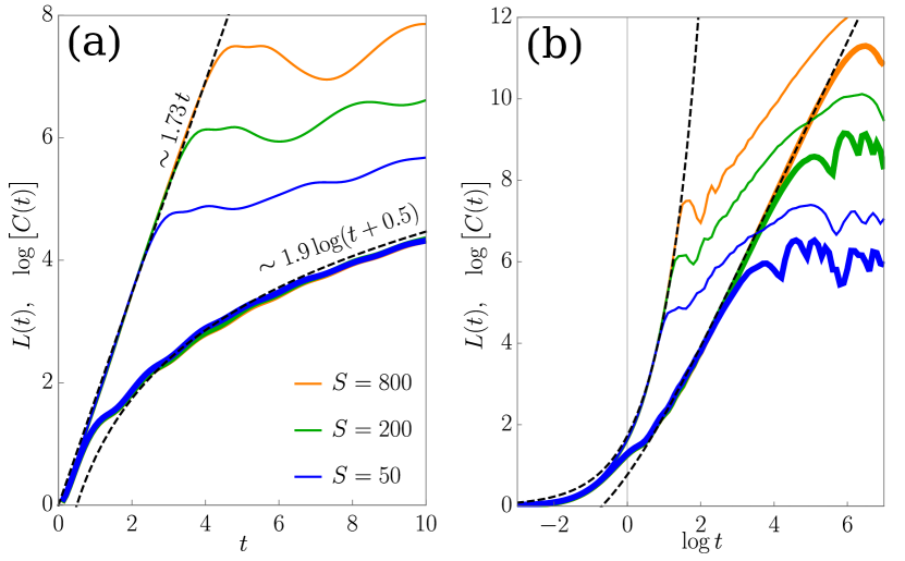
Figure 1: (a) Infinite-temperature OTOCs (thin lines) and LOTOCs (thick lines) in the integrable LMG model. (b) The same plot in the logarithmic timescale.

True chaos.– To study the behavior of the OTOC and the LOTOC in a truly chaotic system, we consider the Feingold-Peres (FP) model [77, 78, 79]:

$$\hat{H}_{\mathrm{FP}}=\hat{x}_{1}+\hat{x}_{2}+4\hat{z}_{1}\hat{z}_{2},$$ (8)

where $(\hat{x}_{i},\hat{y}_{i},\hat{z}_{i})$ are independent rescaled $SU(2)$ spin operators. In the classical limit $S\to\infty$, this model has positive LEs for the majority of initial conditions, see Fig. 2(a). In other words, the phase-space average of classical LEs $\bar{\kappa}_{cl}\approx 0.53>0$, so this system is considered classically chaotic. Moreover, model (8) has two isolated saddle points $x_{1}=x_{2}=\pm 1$, at the vicinity of which $\partial z_{i}(t)/\partial z_{j}(0)\sim e^{\kappa_{s}t}$ with $\kappa_{s}=\sqrt{3}$. We emphasize that $\max\!\left[\kappa_{cl}\right]\approx\kappa_{s}/2>\bar{\kappa}_{cl}$ because “overly chaotic” regions take only a small fraction of the phase space.

The numerical calculation, Fig. 2(b), confirms the qualitative difference between truly chaotic systems and integrable systems with isolated saddle points. In a chaotic system, both OTOC and LOTOC grow according to a chaotic pattern until the “chaotic” Ehrenfest time: $C(t)\sim e^{2\kappa_{q}t}$ and $L(t)\approx 2\bar{\kappa}_{q}t$ for $1\lesssim t\lesssim\log(1/\hbar)$. Furthermore, the LOTOC reproduces the average classical LE, $\bar{\kappa}_{q}\approx\bar{\kappa}_{cl}$, whereas the OTOC grasps only the contribution from the saddle points, $\kappa_{q}\approx\kappa_{s}/2$. This again confirms that the LOTOC correctly describes the semiclassical behavior of a quantized Hamiltonian system.

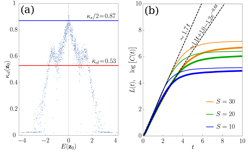
Figure 2: (a) Classical LEs vs. energies for 1250 randomly generated initial conditions in the chaotic classical FP model. (b) Infinite-temperature OTOCs (thin lines) and LOTOCs (thick lines) in the quantum FP model.

Another prominent example of a truly chaotic system is the quantized Arnold cat map [80, 81, 82, 83]. In this model, the LOTOC also correctly reproduces the Ehrenfest time, $t_{E}\sim\log(1/\hbar)$, and the classical LE, $\bar{\kappa}_{q}\approx\bar{\kappa}_{cl}$, see [72].

Many-body chaos.– To illustrate the replica trick (4), we consider the system of $N\gg 1$ nonlinearly coupled oscillators, which is inspired by the spatial reduction of the $SU(2)$ Yang-Mills model [84, 85, 86, 87]:

$$\hat{H}=\left[\frac{1}{2}\hat{p}_{i}^{2}+\frac{1}{2}m^{2}\hat{x}_{i}^{2}+\frac{\lambda}{4N}\hat{x}_{i}^{2}\hat{x}_{j}^{2}\right]-\frac{\lambda}{4N}\hat{x}_{i}^{4},$$ (9)

where we assume the summation over the repeated indices and single out the $O(N)$-symmetric part. The classical counterpart of this model is chaotic for $N\geq 2$, and the average classical LE is estimated as $\bar{\kappa}_{cl}\approx 0.7\sqrt[4]{\lambda T}/N$ in the large-$N$ and high-temperature limit [43].

To estimate replica OTOCs, we write down the tree-level correlation functions on the $2n$-fold Keldysh contour and resum the loop corrections. The leading in $1/N$ corrections preserve the $O(N)$ symmetry; so, in this approximation, model (9) is approximately integrable, and replica OTOCs simply oscillate with time. Nevertheless, the next-to-leading order in $1/N$ contains the contributions from the nonsymmetric vertices that modify the Dyson-Schwinger equation on the resummed replica OTOC. Substituting an exponentially growing ansatz $C_{n}(t)\sim e^{2n\varkappa_{n}t}$ into this equation, we reduce it to the equation on $\varkappa_{n}$:

$$1\approx(2n-1)!!\left[-\frac{1536}{N^{2}}\frac{\lambda^{2}}{(\tilde{\mu}\tilde{m})^{6}}\frac{e^{\tilde{\beta}\tilde{m}}}{\big{(}e^{\tilde{\beta}\tilde{m}}-1\big{)}^{2}}\frac{\tilde{m}^{4}}{\big{(}\tilde{m}^{2}+\varkappa_{n}^{2}\big{)}^{2}}\right]^{n}.$$ (10)

The leading contribution to this equation is ensured by the “mixed multi-rung” ladder diagrams (Fig. 3). For brevity, we introduce short notations for the inverse temperature of the replicated model $\tilde{\beta}=(n+1)/T$, the resummed mass $\tilde{m}$, and the parameter of the resummed vertex $\tilde{\mu}$. The solution to Eq. (10) gives an approximate expression for the replica LE:

$$\kappa_{n}=n\varkappa_{n}\approx n\left[(2n-1)!!\right]^{\frac{1}{2n}}\frac{8\sqrt{6}}{N}\frac{\lambda\tilde{m}}{(\tilde{\mu}\tilde{m})^{3}}\frac{e^{\tilde{\beta}\tilde{m}/2}}{e^{\tilde{\beta}\tilde{m}}-1}.$$ (11)

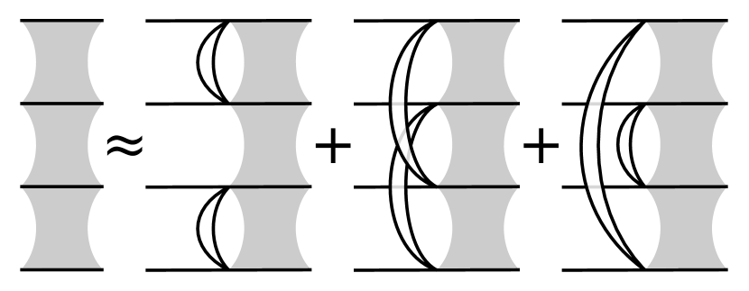
Figure 3: The approximate Dyson-Schwinger equation that sums the leading exponentially growing contributions to $C_{2}(t)$ in model (9). Horizontal lines denote retarded propagators on different folds of the Keldysh contour, and vertical crescents denote resummed bubble chains that connect symmetric and nonsymmetric vertices on different folds.

Finally, employing the replica trick (4), we estimate the refined quantum LE in the high-temperature and weak-coupling limit, $m/T\ll\lambda/m^{3}\ll 1$:

$$\bar{\kappa}_{q}\approx 0.7\sqrt[4]{\lambda T}/N.$$ (12)

We emphasize that the refined quantum LE is approximately two times smaller than the conventional LE, $\kappa_{q}\approx 1.3\sqrt[4]{\lambda T}/N$. From the diagrammatic perspective, the refined quantum LE is reduced by correlations between different replicas, which do not factorize and leave footprints in the behavior of the LOTOC (Fig. 3). From the semiclassical perspective, the discrepancy arises because classical LEs have a nontrivial distribution in the phase space (Fig. 4). The LOTOC measures the fair average of LEs, so $\bar{\kappa}_{q}\approx\bar{\kappa}_{cl}$ as $\hbar\to 0$; on the contrary, the OTOC selects only the points with the largest LEs, so $\kappa_{q}\approx\max\left[\kappa_{cl}(\mathbf{z}_{0})\right]>\bar{\kappa}_{cl}$ as $\hbar\to 0$, where the maximum is taken over all initial conditions $\mathbf{z}_{0}$. In this respect, model (9) is similar to the FP model, where the average and maximum classical LEs also differ, cf. Fig. 2(a).

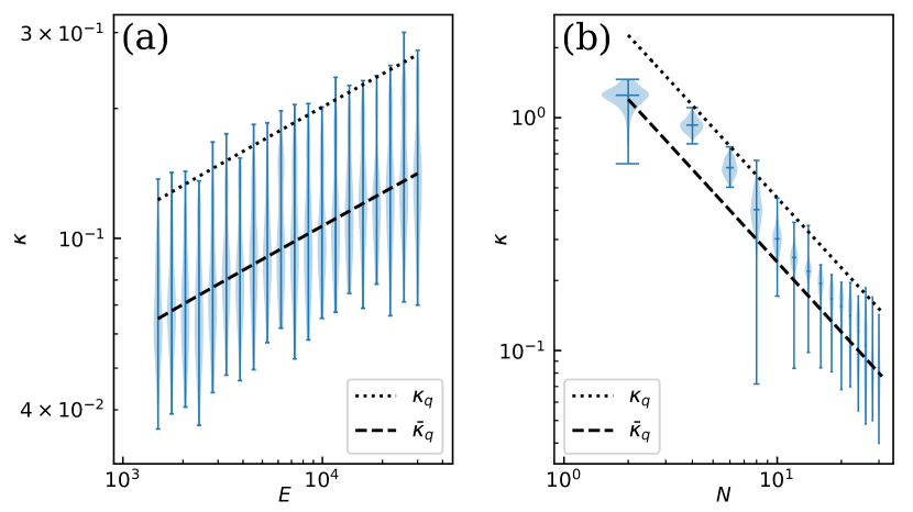
Figure 4: Numerically calculated classical LEs $\kappa_{cl}$ (vertical bars and violins), conventional quantum LEs $\kappa_{q}$, and refined quantum LEs $\bar{\kappa}_{q}$ for a fixed number of oscillators $N=30$ (a) or energy $E=100m^{4}/\lambda$ (b) in model (9).

Maximal chaos.– Maximally chaotic quantum systems, where OTOCs exponentially grow with time and saturate the bound [2], are especially notable for their putative duality to black holes. The Sachdev-Ye-Kitaev (SYK) model is probably the most prominent example of such a system. This is a quantum mechanical model of $N$ Majorana fermions $\chi_{i}$ with all-to-all random couplings [25, 26, 27, 28, 29, 30]:

$$\hat{H}_{\mathrm{SYK}}=i^{q/2}\sum_{1\leq k_{1}\leq\cdots\leq k_{q}\leq N}j_{k_{1}\cdots k_{q}}\chi_{k_{1}}\cdots\chi_{k_{q}},$$ (13)

where numbers $j_{k_{1}\cdots k_{q}}$ are drawn from a Gaussian distribution with zero mean and the following variance:

$$\left\langle j_{k_{1}\cdots k_{q}}^{2}\right\rangle=\frac{2^{q-1}}{q}\frac{J^{2}(q-1)!}{N^{q-1}}\quad\text{(no sum)}.$$ (14)

Let us calculate the refined quantum LE of the SYK model and show that it saturates the bound [2] similarly to the conventional quantum LE. For simplicity, we consider the limit $N\gg q\gg 1$, where the leading contributions to the exact propagators are calculated explicitly. To estimate these contributions, we first solve the Dyson-Schwinger equation on the Euclidean propagator that lives on the imaginary-time part of the $2n$-fold Keldysh contour. In the limit $N\gg q\gg 1$, this equation resums the melonic diagrams and has the following approximate solution:

$$G(\tau)\approx\frac{1}{2}\mathrm{sgn}(\tau)\left[1+\frac{2}{q}\log\frac{\cos\frac{\pi\tilde{v}}{2}}{\cos\left(\frac{\pi\tilde{v}}{2}-\frac{\pi\tilde{v}|\tau|}{\tilde{\beta}}\right)}\right],$$ (15)

where the parameter $\tilde{v}$ is determined from the equation $\tilde{\beta}J=\pi\tilde{v}/\cos\left(\pi\tilde{v}/2\right)$ and $\tilde{\beta}=(n+1)/T$ is the inverse temperature of the replicated model. Analytically continuing propagator (15) to real times, we obtain all propagators on the $2n$-fold Keldysh contour. Then, similarly to model (9), we write down the Dyson-Schwinger equation on the resummed replica OTOC (Fig. 5), substitute the ansatz $C_{n}(t)\sim e^{2n\varkappa_{n}t}$, and obtain the equation on $\varkappa_{n}$:

$$1\approx\left[2\pi\tilde{v}/\tilde{\beta}\varkappa_{n}\right]^{n}.$$ (16)

Note that Eqs. (10) and (16) have different combinatorial prefactors due to the peculiarities of the large-$N$ limits in models (9) and (13). Finally, solving Eq. (16) and substituting the solution into Eq. (4), we obtain the refined quantum LE in the limit in question:

$$\bar{\kappa}_{q}=2\pi Tv,$$ (17)

where the parameter $v$ is determined from the equation $J/T=\pi v/\cos(\pi v/2)$.

We emphasize that in the SYK model, refined and conventional quantum LEs coincide because correlations between different folds of the Keldysh contour are suppressed by the powers of $1/N$, see Fig. 5. Indeed, the replica OTOCs simply factorize, $C_{n}(t)\sim\left[C_{1}(t)\right]^{n}$, so the replica trick (4) yields $\bar{\kappa}_{q}=\lim\varkappa_{n}=\kappa_{q}$. In particular, this implies that the refined quantum LE (17) saturates the bound $\bar{\kappa}_{q}\leq 2\pi T$ in the low-temperature limit $T\ll J$.

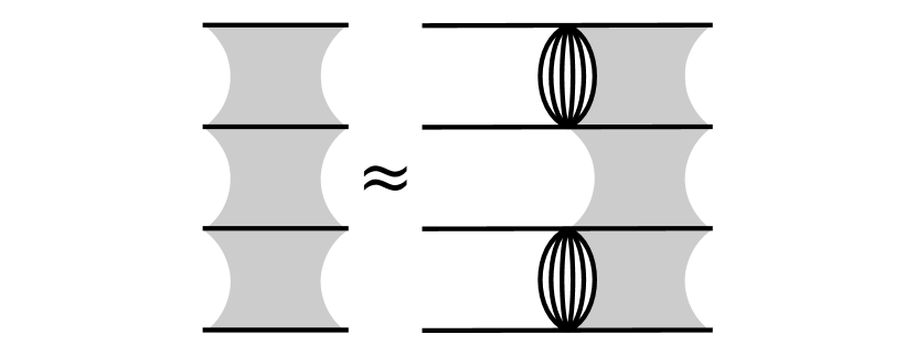
Figure 5: The approximate Dyson-Schwinger equation that sums the leading exponentially growing contributions to $C_{2}(t)$ in the SYK model with $q=8$. Horizontal lines denote retarded propagators, and vertical lines denote Wightman propagators that connect different folds of the Keldysh contour.

A bound on refined chaos.– One of the most important achievements of OTOCs is the bound on quantum LE [2], $\kappa_{q}\leq 2\pi T$, which resolves the cloning paradox [17, 18, 19] and helps to find holographic duals of black holes. We argue that the refined quantum LE also satisfies this bound.

First, the semiclassical picture discussed in the previous sections implies that the refined quantum LE coincides with the phase-space average of classical LEs, whereas the conventional quantum LE approaches the phase-space supremum of classical LEs as $\hbar\to 0$. Since the average cannot be greater than the maximum element of the set, the refined quantum LE is less than or equal to the conventional one. Hence, it automatically satisfies the bound $\bar{\kappa}_{q}\leq\kappa_{q}\leq 2\pi T$.

Second, the replica LEs are proved to satisfy the bound $\kappa_{n}\leq 2\pi Tn$ for any positive integer $n$ [88, 89]. Analytically continuing this inequality to real $n$, keeping in mind that $\kappa_{n}\geq 0$ by definition, and employing a variant of the replica trick (4), $\bar{\kappa}_{q}\to\left(\kappa_{n}-\kappa_{0}\right)/n$ as $n\to 0$, we straightforwardly obtain the bound $\bar{\kappa}_{q}\leq 2\pi T$.

Finally, calculations in the SYK model, which is dual to the nearly-AdS₂ gravity with matter [31, 32, 33, 34, 35], show that the refined and conventional quantum LEs can coincide and saturate the bound [2] together. Hence, the saturation of the inequality $\bar{\kappa}_{q}\leq 2\pi T$ is still a useful indicator of the gauge/gravity duality.

Discussion.– We have shown that the LOTOC correctly describes the semiclassical behavior of quantized Hamiltonian systems. Unlike the conventional OTOC, it correctly reproduces the Ehrenfest time and the average classical LE in both chaotic and integrable systems, including systems with isolated saddle points. Of course, our case studies are by no means exhaustive. In particular, it is very interesting to examine the behavior of the LOTOC after the Ehrenfest time. However, our examples make it sufficiently clear that the LOTOC provides a proper definition of quantum chaos and quantum butterfly effect — the exponential sensitivity to typical small perturbations ensured by $\bar{\kappa}_{q}>0$, — and correctly reproduces the definition of classical chaos in the limit $\hbar\to 0$.

At the same time, the LOTOC retains all advantages of the OTOC. In particular, it can be calculated analytically employing the replica trick and the extended Schwinger-Keldysh diagram technique, which are especially useful for large-$N$ quantum systems dual to black holes. Moreover, the refined quantum LE satisfies the fundamental bound on chaos, $\bar{\kappa}_{q}\leq\kappa_{q}\leq 2\pi T$. So, in a sense, our approach reconciles the definitions of quantum chaos and scrambling separated by the observations of [54]. Besides, the LOTOC and the replica OTOCs can be experimentally measured using the same protocols as conventional OTOCs [20, 21, 22, 23, 24]. Thus, the LOTOC fixes the flaws of conventional OTOCs, where these flaws are important, and has a comparably wide range of applications, from thermalization of quantum systems to teleportation through a traversable wormhole (e.g., see [21, 90, 91]).

Acknowledgments.– We thank Nikita Kolganov and Artem Alexandrov for the collaboration at the initial stage of this project. We are also grateful to Anatoly Dymarsky, Elizaveta Trunina, Andrei Semenov, Vladimir Losyakov, Petr Arseev, Damir Sadekov, and Alexey Rubtsov for valuable discussions. The classical LEs at Fig. 2(a) were calculated using package [92]. This work was supported by the Foundation for the Advancement of Theoretical Physics and Mathematics “BASIS”.

References

- Larkin and Ovchinnikov [1969] A. I. Larkin and Y. N. Ovchinnikov, Quasiclassical method in the theory of superconductivity, Sov. Phys. JETP 28, 1200 (1969), [Zh. Eksp. Teor. Fiz. 55, 2262 (1968)].
- Maldacena et al. [2016a] J. Maldacena, S. H. Shenker, and D. Stanford, A bound on chaos, J. High Energy Phys. 2016 (08), 106, arXiv:1503.01409 .
- [3] A. Kitaev, A simple model of quantum holography, KITP seminar, April 7, 2015 and May 7, 2015.
- Swingle [2018] B. Swingle, Unscrambling the physics of out-of-time-order correlators, Nature Phys. 14, 988 (2018).
- García-Mata et al. [2023] I. García-Mata, R. A. Jalabert, and D. A. Wisniacki, Out-of-time-order correlators and quantum chaos, Scholarpedia 18, 55237 (2023), arXiv:2209.07965 .
- Note [1] We consider a Hamiltonian system and introduce the canonical coordinates on the phase space .
- Shenker and Stanford [2014a] S. H. Shenker and D. Stanford, Black holes and the butterfly effect, J. High Energy Phys. 2014 (03), 067, arXiv:1306.0622 .
- Shenker and Stanford [2014b] S. H. Shenker and D. Stanford, Multiple shocks, J. High Energy Phys. 2014 (12), 046, arXiv:1312.3296 .
- Roberts et al. [2015] D. A. Roberts, D. Stanford, and L. Susskind, Localized shocks, J. High Energy Phys. 2015 (03), 051, arXiv:1409.8180 .
- Shenker and Stanford [2015] S. H. Shenker and D. Stanford, Stringy effects in scrambling, J. High Energy Phys. 2015 (05), 132, arXiv:1412.6087 .
- Swingle et al. [2016] B. Swingle, G. Bentsen, M. Schleier-Smith, and P. Hayden, Measuring the scrambling of quantum information, Phys. Rev. A 94, 040302 (2016), arXiv:1602.06271 .
- Roberts and Swingle [2016] D. A. Roberts and B. Swingle, Lieb-Robinson bound and the butterfly effect in quantum field theories, Phys. Rev. Lett. 117, 091602 (2016), arXiv:1603.09298 .
- Nahum et al. [2018] A. Nahum, S. Vijay, and J. Haah, Operator spreading in random unitary circuits, Phys. Rev. X 8, 021014 (2018), arXiv:1705.08975 .
- Mi et al. [2021] X. Mi et al., Information scrambling in quantum circuits, Science 374, 1479 (2021), arXiv:2101.08870 .
- Xu and Swingle [2019] S. Xu and B. Swingle, Accessing scrambling using matrix product operators, Nature Phys. 16, 199 (2019), arXiv:1802.00801 .
- [16] S. Xu and B. Swingle, Scrambling dynamics and out-of-time ordered correlators in quantum many-body systems: a tutorial, arXiv:2202.07060 .
- Hayden and Preskill [2007] P. Hayden and J. Preskill, Black holes as mirrors: Quantum information in random subsystems, J. High Energy Phys. 2007 (09), 120, arXiv:0708.4025 .
- Sekino and Susskind [2008] Y. Sekino and L. Susskind, Fast scramblers, J. High Energy Phys. 2008 (10), 065, arXiv:0808.2096 .
- Lashkari et al. [2013] N. Lashkari, D. Stanford, M. Hastings, T. Osborne, and P. Hayden, Towards the fast scrambling conjecture, J. High Energy Phys. 2013 (04), 022, arXiv:1111.6580 .
- García-Álvarez et al. [2017] L. García-Álvarez, I. L. Egusquiza, L. Lamata, A. del Campo, J. Sonner, and E. Solano, Digital quantum simulation of minimal AdS/CFT, Phys. Rev. Lett. 119, 040501 (2017), arXiv:1607.08560 .
- Jafferis et al. [2022] D. Jafferis, A. Zlokapa, J. D. Lykken, D. K. Kolchmeyer, S. I. Davis, N. Lauk, H. Neven, and M. Spiropulu, Traversable wormhole dynamics on a quantum processor, Nature 612, 51 (2022).
- Gärttner et al. [2017] M. Gärttner, J. G. Bohnet, A. Safavi-Naini, M. L. Wall, J. J. Bollinger, and A. M. Rey, Measuring out-of-time-order correlations and multiple quantum spectra in a trapped ion quantum magnet, Nature Phys. 13, 781 (2017), arXiv:1608.08938 .
- Li et al. [2017] J. Li, R. Fan, H. Wang, B. Ye, B. Zeng, H. Zhai, X. Peng, and J. Du, Measuring out-of-time-order correlators on a nuclear magnetic resonance quantum simulator, Phys. Rev. X 7, 031011 (2017), arXiv:1609.01246 .
- Green et al. [2022] A. M. Green, A. Elben, C. H. Alderete, L. K. Joshi, N. H. Nguyen, T. V. Zache, Y. Zhu, B. Sundar, and N. M. Linke, Experimental measurement of out-of-time-ordered correlators at finite temperature, Phys. Rev. Lett. 128, 140601 (2022), arXiv:2112.02068 .
- Polchinski and Rosenhaus [2016] J. Polchinski and V. Rosenhaus, The spectrum in the Sachdev-Ye-Kitaev model, J. High Energy Phys. 2016 (04), 001, arXiv:1601.06768 .
- Maldacena and Stanford [2016] J. Maldacena and D. Stanford, Remarks on the Sachdev-Ye-Kitaev model, Phys. Rev. D 94, 106002 (2016), arXiv:1604.07818 .
- Kitaev and Suh [2018] A. Kitaev and S. J. Suh, The soft mode in the Sachdev-Ye-Kitaev model and its gravity dual, J. High Energy Phys. 2018 (05), 183, arXiv:1711.08467 .
- Sárosi [2018] G. Sárosi, AdS2 holography and the SYK model, PoS Modave2017, 001 (2018), arXiv:1711.08482 .
- Rosenhaus [2019] V. Rosenhaus, An introduction to the SYK model, J. Phys. A 52, 323001 (2019), arXiv:1807.03334 .
- Trunin [2021] D. A. Trunin, Pedagogical introduction to the Sachdev-Ye-Kitaev model and two-dimensional dilaton gravity, Phys. Usp. 64, 219 (2021), [Usp. Fiz. Nauk 191, 225 (2021)], arXiv:2002.12187 .
- Maldacena et al. [2016b] J. Maldacena, D. Stanford, and Z. Yang, Conformal symmetry and its breaking in two dimensional nearly anti-de Sitter space, Prog. Theor. Exp. Phys. 2016, 12C104 (2016b), arXiv:1606.01857 .
- Jensen [2016] K. Jensen, Chaos in AdS2 Holography, Phys. Rev. Lett. 117, 111601 (2016), arXiv:1605.06098 .
- Engelsöy et al. [2016] J. Engelsöy, T. G. Mertens, and H. Verlinde, An investigation of AdS2 backreaction and holography, J. High Energy Phys. 2016 (07), 139, arXiv:1606.03438 .
- Gross and Rosenhaus [2017a] D. J. Gross and V. Rosenhaus, The bulk dual of SYK: cubic couplings, J. High Energy Phys. 2017 (05), 092, arXiv:1702.08016 .
- Gross and Rosenhaus [2017b] D. J. Gross and V. Rosenhaus, All point correlation functions in SYK, J. High Energy Phys. 2017 (12), 148, arXiv:1710.08113 .
- Roberts and Stanford [2015] D. A. Roberts and D. Stanford, Two-dimensional conformal field theory and the butterfly effect, Phys. Rev. Lett. 115, 131603 (2015), arXiv:1412.5123 .
- Fitzpatrick and Kaplan [2016] A. L. Fitzpatrick and J. Kaplan, A quantum correction to chaos, J. High Energy Phys. 2016 (05), 070, arXiv:1601.06164 .
- Turiaci and Verlinde [2016] G. Turiaci and H. Verlinde, On CFT and quantum chaos, J. High Energy Phys. 2016 (12), 110, arXiv:1603.03020 .
- Stanford [2016] D. Stanford, Many-body chaos at weak coupling, J. High Energy Phys. 2016 (10), 009, arXiv:1512.07687 .
- Grozdanov et al. [2019] S. Grozdanov, K. Schalm, and V. Scopelliti, Kinetic theory for classical and quantum many-body chaos, Phys. Rev. E 99, 012206 (2019), arXiv:1804.09182 .
- Hashimoto et al. [2017] K. Hashimoto, K. Murata, and R. Yoshii, Out-of-time-order correlators in quantum mechanics, J. High Energy Phys. 2017 (10), 138, arXiv:1703.09435 .
- Akutagawa et al. [2020] T. Akutagawa, K. Hashimoto, T. Sasaki, and R. Watanabe, Out-of-time-order correlator in coupled harmonic oscillators, J. High Energy Phys. 2020 (08), 013, arXiv:2004.04381 .
- Kolganov and Trunin [2022] N. Kolganov and D. A. Trunin, Classical and quantum butterfly effect in nonlinear vector mechanics, Phys. Rev. D 106, 025003 (2022), arXiv:2205.05663 .
- Buividovich et al. [2019] P. V. Buividovich, M. Hanada, and A. Schäfer, Quantum chaos, thermalization, and entanglement generation in real-time simulations of the Banks-Fischler-Shenker-Susskind matrix model, Phys. Rev. D 99, 046011 (2019), arXiv:1810.03378 .
- Buividovich [2022] P. V. Buividovich, Quantum chaos in supersymmetric quantum mechanics: An exact diagonalization study, Phys. Rev. D 106, 046001 (2022), arXiv:2205.09704 .
- Bohrdt et al. [2017] A. Bohrdt, C. B. Mendl, M. Endres, and M. Knap, Scrambling and thermalization in a diffusive quantum many-body system, New J. Phys. 19, 063001 (2017), arXiv:1612.02434 .
- Klug et al. [2018] M. J. Klug, M. S. Scheurer, and J. Schmalian, Hierarchy of information scrambling, thermalization, and hydrodynamic flow in graphene, Phys. Rev. B 98, 045102 (2018), arXiv:1712.08813 .
- Chowdhury and Swingle [2017] D. Chowdhury and B. Swingle, Onset of many-body chaos in the model, Phys. Rev. D 96, 065005 (2017), arXiv:1703.02545 .
- Patel et al. [2017] A. A. Patel, D. Chowdhury, S. Sachdev, and B. Swingle, Quantum butterfly effect in weakly interacting diffusive metals, Phys. Rev. X 7, 031047 (2017), arXiv:1703.07353 .
- Tikhanovskaya et al. [2022] M. Tikhanovskaya, S. Sachdev, and A. A. Patel, Maximal quantum chaos of the critical fermi surface, Phys. Rev. Lett. 129, 060601 (2022), arXiv:2202.01845 .
- Kent et al. [2023] B. Kent, S. Racz, and S. Shashi, Scrambling in quantum cellular automata, Phys. Rev. B 107, 144306 (2023), arXiv:2301.07722 .
- Rozenbaum et al. [2017] E. B. Rozenbaum, S. Ganeshan, and V. Galitski, Lyapunov exponent and out-of-time-ordered correlator’s growth rate in a chaotic system, Phys. Rev. Lett. 118, 086801 (2017), arXiv:1609.01707 .
- Rozenbaum et al. [2020] E. B. Rozenbaum, L. A. Bunimovich, and V. Galitski, Early-time exponential instabilities in nonchaotic quantum systems, Phys. Rev. Lett. 125, 014101 (2020), arXiv:1902.05466 .
- Xu et al. [2020] T. Xu, T. Scaffidi, and X. Cao, Does scrambling equal chaos?, Phys. Rev. Lett. 124, 140602 (2020), arXiv:1912.11063 .
- Pilatowsky-Cameo et al. [2020] S. Pilatowsky-Cameo, J. Chávez-Carlos, M. A. Bastarrachea-Magnani, P. Stránský, S. Lerma-Hernández, L. F. Santos, and J. G. Hirsch, Positive quantum Lyapunov exponents in experimental systems with a regular classical limit, Phys. Rev. E 101, 010202 (2020), arXiv:1909.02578 .
- Wang and Pérez-Bernal [2019] Q. Wang and F. Pérez-Bernal, Probing an excited-state quantum phase transition in a quantum many-body system via an out-of-time-order correlator, Phys. Rev. A 100, 062113 (2019), arXiv:1812.01920 .
- Pappalardi et al. [2018] S. Pappalardi, A. Russomanno, B. Žunkovič, F. Iemini, A. Silva, and R. Fazio, Scrambling and entanglement spreading in long-range spin chains, Phys. Rev. B 98, 134303 (2018), arXiv:1806.00022 .
- Hummel et al. [2019] Q. Hummel, B. Geiger, J. D. Urbina, and K. Richter, Reversible quantum information spreading in many-body systems near criticality, Phys. Rev. Lett. 123, 160401 (2019), arXiv:1812.09237 .
- Hashimoto et al. [2020] K. Hashimoto, K.-B. Huh, K.-Y. Kim, and R. Watanabe, Exponential growth of out-of-time-order correlator without chaos: inverted harmonic oscillator, J. High Energy Phys. 2020 (11), 068, arXiv:2007.04746 .
- [60] M. Steinhuber, P. Schlagheck, J.-D. Urbina, and K. Richter, A dynamical transition from localized to uniform scrambling in locally hyperbolic systems, arXiv:2303.14839 .
- [61] N. Dowling, P. Kos, and K. Modi, Scrambling is necessary but not sufficient for chaos, arXiv:2304.07319 .
- Note [2] Note that the operator under logarithm is Hermitian and positive definite, so the logarithm is well defined.
- Shepelyansky [2020] D. Shepelyansky, Ehrenfest time and chaos, Scholarpedia 15, 55031 (2020).
- Zaslavsky [1981] G. M. Zaslavsky, Stochasticity in quantum systems, Phys. Rep. 80, 157 (1981).
- Chirikov et al. [1988] B. V. Chirikov, F. M. Izrailev, and D. L. Shepelyansky, Quantum chaos: localization vs. ergodicity, Physica D 33, 77 (1988).
- Aleiner and Larkin [1996] I. L. Aleiner and A. I. Larkin, Divergence of classical trajectories and weak localization, Phys. Rev. B 54, 14423 (1996), arXiv:cond-mat/9603121 .
- Tabor [1989] M. Tabor, Chaos and Integrability in Nonlinear Dynamics: an Introduction (Wiley-Interscience, 1989).
- Pesin [1977] Y. B. Pesin, Characteristic Lyapunov exponents and smooth ergodic theory, Russ. Math. Surv. 32, 55 (1977), [Usp. Mat. Nauk 32, 55 (1977)].
- Aleiner et al. [2016] I. L. Aleiner, L. Faoro, and L. B. Ioffe, Microscopic model of quantum butterfly effect: out-of-time-order correlators and traveling combustion waves, Annals Phys. 375, 378 (2016), arXiv:1609.01251 .
- Haehl et al. [2019] F. M. Haehl, R. Loganayagam, P. Narayan, and M. Rangamani, Classification of out-of-time-order correlators, SciPost Phys. 6, 001 (2019), arXiv:1701.02820 .
- Romero-Bermúdez et al. [2019] A. Romero-Bermúdez, K. Schalm, and V. Scopelliti, Regularization dependence of the OTOC. Which Lyapunov spectrum is the physical one?, J. High Energy Phys. 2019 (07), 107, arXiv:1903.09595 .
- [72] D. A. Trunin, Refined quantum Lyapunov exponents from replica out-of-time-order correlators, arXiv:2308.02392 .
- Lipkin et al. [1965] H. J. Lipkin, N. Meshkov, and A. J. Glick, Validity of many-body approximation methods for a solvable model: (I). Exact solutions and perturbation theory, Nucl. Phys. 62, 188 (1965).
- Meshkov et al. [1965] N. Meshkov, A. J. Glick, and H. J. Lipkin, Validity of many-body approximation methods for a solvable model: (II). Linearization procedures, Nucl. Phys. 62, 199 (1965).
- Glick et al. [1965] A. J. Glick, H. J. Lipkin, and N. Meshkov, Validity of many-body approximation methods for a solvable model: (III). Diagram summations, Nucl. Phys. 62, 211 (1965).
- Note [3] On a Kähler manifold, classical LEs do not depend on the space parametrization, and we believe this property to be preserved after the semiclassical quantization.
- Feingold and Peres [1983] M. Feingold and A. Peres, Regular and chaotic motion of coupled rotators, Physica D 9, 433 (1983).
- Feingold et al. [1984] M. Feingold, N. Moiseyev, and A. Peres, Ergodicity and mixing in quantum theory. II, Phys. Rev. A 30, 509 (1984).
- Fan et al. [2017] Y. Fan, S. Gnutzmann, and Y. Liang, Quantum chaos for nonstandard symmetry classes in the Feingold-Peres model of coupled tops, Phys. Rev. E 96, 062207 (2017), arXiv:1709.03584 .
- Esposti and Graffi [2003] M. D. Esposti and S. Graffi, Mathematical aspects of quantum maps, in Mathematical Aspects of Quantum Maps, Lecture Notes in Physics, Vol 618. (Springer-Verlag, Berlin Heidelberg, 2003) p. 49.
- Hannay and Berry [1980] J. H. Hannay and M. V. Berry, Quantization of linear maps on a torus-Fresnel diffraction by a periodic grating, Physica D 1, 267 (1980).
- García-Mata et al. [2018] I. García-Mata, M. Saraceno, R. A. Jalabert, A. J. Roncaglia, and D. A. Wisniacki, Chaos signatures in the short and long time behavior of the out-of-time ordered correlator, Phys. Rev. Lett. 121, 210601 (2018), arXiv:1806.04281 .
- Moudgalya et al. [2019] S. Moudgalya, T. Devakul, C. W. von Keyserlingk, and S. L. Sondhi, Operator spreading in quantum maps, Phys. Rev. B 99, 094312 (2019), arXiv:1808.04889 .
- Matinyan et al. [1981] S. G. Matinyan, G. K. Savvidy, and N. G. Ter-Arutunian-Savvidy, Classical Yang-Mills mechanics. Nonlinear color oscillations, Sov. Phys. JETP 53, 421 (1981), [Zh. Eksp. Teor. Fiz. 80, 830 (1981)].
- Chirikov and Shepelyansky [1981] B. V. Chirikov and D. L. Shepelyansky, Stochastic oscillations of classical Yang-Mills fields, JETP Lett. 34, 171 (1981), [Pis’ma Zh. Eksp. Teor. Fiz. 34, 171 (1981)].
- Savvidy [1984] G. K. Savvidy, Classical and quantum mechanics of nonabelian gauge fields, Nucl. Phys. B 246, 302 (1984).
- Savvidy [2022] G. Savvidy, Maximally chaotic dynamical systems of Anosov–Kolmogorov and fundamental interactions, Int. J. Mod. Phys. A 37, 2230001 (2022), arXiv:2202.09846 .
- Pappalardi and Kurchan [2023] S. Pappalardi and J. Kurchan, Quantum bounds on the generalized Lyapunov exponents, Entropy 25, 246 (2023), arXiv:2212.10123 .
- Tsuji et al. [2018] N. Tsuji, T. Shitara, and M. Ueda, Bound on the exponential growth rate of out-of-time-ordered correlators, Phys. Rev. E 98, 012216 (2018), arXiv:1706.09160 .
- [90] B. Yoshida and A. Kitaev, Efficient decoding for the Hayden-Preskill protocol, arXiv:1710.03363 .
- Gao and Jafferis [2021] P. Gao and D. L. Jafferis, A traversable wormhole teleportation protocol in the SYK model, J. High Energy Phys. 2021 (07), 097, arXiv:1911.07416 .
- Sandri [1996] M. Sandri, Numerical calculation of Lyapunov exponents, Mathematica J. 6, 78 (1996).