Isolated zero mode in a quantum computer from a duality twist

Sutapa Samanta Affiliation: Department of Physics and Astronomy, Western Washington University, Bellingham, Washington 98225, USA    Derek S. Wang Affiliation: IBM Quantum, IBM T.J. Watson Research Center, Yorktown Heights, New York 10598, USA    Armin Rahmani Affiliation: Department of Physics and Astronomy, Western Washington University, Bellingham, Washington 98225, USA Affiliation: Advanced Materials Science and Engineering Center, Western Washington University, Bellingham, Washington 98225, USA    Aditi Mitra Affiliation: Center for Quantum Phenomena, Department of Physics, New York University, 726 Broadway, New York, New York 10003, USA
Abstract

Investigating the interplay of dualities, generalized symmetries, and topological defects beyond theoretical models is an important challenge in condensed matter physics and quantum materials. A simple model exhibiting this physics is the transverse-field Ising model, which can host atopological defect that performs the Kramers-Wannier duality transformation. When acting on one point in space, this duality defect imposes the duality twisted boundary condition and binds a single zero mode. This zero mode is unusual as it lacks a localized partner in the same Z2Z_{2} sector and has an infinite lifetime, even in finite systems. Using Floquet driving of a closed Ising chain with a duality defect, we generate this zero mode in a digital quantum computer. We detect the mode by measuring its associated persistent autocorrelation function using an efficient sampling protocol and a compound strategy for error mitigation. We also show that the zero mode resides at the domain wall between two regions related by a Kramers-Wannier duality transformation. Finally, we highlight the robustness of the isolated zero mode to integrability- and symmetry-breaking perturbations. Our findings provide a method for exploring exotic topological defects, associated with noninvertible generalized symmetries, in digitized quantum devices.

I Introduction

Symmetry is a cornerstone of modern physics. Traditionally, symmetries in quantum systems are realized as unitary representations of a group of transformations that leave the Hamiltonian invariant. Dualities are transformations that relate two different models, or different phases of the same model, and are closely related to symmetry but cannot always be described within the traditional framework Cobanera et al. 2011; Seiberg et al. 2016; Somoza et al. 2021; Lootens et al. 2021. Duality transformations can act as projectors, which do not admit a unitary representation but are examples of noninvertible symmetries Verlinde 1988; Bhardwaj et al. 2023; Aasen et al. 2016; Thorngren and Wang 2019; Aasen et al. 2020. Both unitary (invertible) and noninvertible symmetries are described within the recently developed framework of generalized symmetries Kong et al. 2020; McGreevy 2022, and can manifest through topological defects Gaiotto et al. 2015; Aasen et al. 2016; Aasen et al. 2020; Gaiotto et al. 2021.

Exploring topological defects, encompassing both invertible and noninvertible types, stands at the forefront of research in condensed matter and high-energy physics Cheng and Seiberg 2023; Eck and Fendley 2023. Despite remarkable theoretical progress, detecting exotic topological defects associated with generalized symmetries is challenging in traditional condensed-matter systems, rendering their experimental realization an open question. Here, we realize such a system on a synthetic platform, a small, noisy quantum computer Preskill 2018.

The Kramers-Wannier duality transformation of the transverse-field Ising model (TFIM) is one of the most well-known dualities Kramers and Wannier 1941. The TFIM can support different topological defects, including the familiar unitary spin-flip defect, which captures the Z2Z_{2} symmetry of the model, and the duality defect Aasen et al. 2016; Aasen et al. 2020; Tan et al. 2024 studied here. The duality defect is one of the simplest examples of a noninvertible transformation as it projects out states of a given Z2Z_{2} symmetry Aasen et al. 2016. A duality defect acting at a particular point in space imposes a special “twisted” boundary condition Cardy 1989; Verlinde 1988; Schutz 1993; Oshikawa and Affleck 1997; Petkova and Zuber 2001; Grimm 2002; Fröhlich et al. 2004; Chang et al. 2019. One of the consequences of the duality defect is the emergence of a zero mode, bound to the defect, with distinct characteristics from more well-known edge zero modes occurring in the TFIM with open boundary conditions Aasen et al. 2016; Tan et al. 2024.

It is well-established that the TFIM with open boundary conditions can host Majorana zero modes Kitaev 2001; Fendley 2016 in the topological phase, both in equilibrium and in its Floquet versions Thakurathi et al. 2013; Yates et al. 2019. These modes appear in pairs localized at the two edges of the system, and have a lifetime which grows exponentially with the system size because they hybridize leading to an energy splitting that is exponentially small in the system size. On the other hand, the zero mode appearing due to a duality twist defect is isolated, lacking a localized partner in the same Z2Z_{2} sector. It thus has an infinite lifetime, even in finite systems. In addition, this isolated mode exists for all couplings of the static and Floquet versions of the TFIM, and separates the chain into two parts whose couplings are related by the Kramers-Wannier duality transformation Aasen et al. 2016; Mitra et al. 2023.

Digitized quantum devices have provided a new playground for realizing topological physics Rahmani et al. 2020; Satzinger et al 2021; Stenger et al. 2021; Liu et al. 2022; Kirmani et al. 2022; Andersen et al 2023; Harle et al. 2023; Kirmani et al. 2023. In particular, Floquet versions of the TFIM with open boundary conditions have been studied on current noisy quantum devices Mi and et al 2022; Harle et al. 2023. In this paper, we probe the Floquet version of the TFIM with a duality twist defect. We implement the duality twist defect in a closed chain of 20 qubits on the ibmq_kolkata device and observe signatures of an isolated zero mode. By obtaining the autocorrelation functions of several operators in the quantum device, we demonstrate that the zero mode, with a theoretically infinite lifetime Tan et al. 2024; Mitra et al. 2023, is persistent. We also confirm that weak perturbations, which break both the integrability and the Z2Z_{2} symmetry of the system, do not destabilize the zero mode in finite-length chains.

We further investigate the properties of this mode by applying a local unitary circuit that moves the twist defect. We observe that the zero mode does not follow the defect but remains in its original position. This contrasts sharply with a potential well that binds a localized mode, where moving the potential well would also translate the localized mode. This behavior is a consequence of the fact that the twist defect is topological, meaning that a local unitary transformation can move the defect, while leaving the Hamiltonian invariant when all the couplings are set equal to each other. For unequal couplings, there are still ramifications of the topological properties of the defect, which will be discussed later. Recall that translations do not fall under the category of local unitary transformations, thus this property is not shared by a chain with a local impurity potential.

The paper is organized as follows. In Section II, we introduce the model and define the autocorrelation function utilized for detecting the zero mode. Sections III, IV, and V are focused on results obtained on the IBM quantum computer. In particular, Sec. III discusses the localized zero mode for the integrable model, Sec. IV demonstrates the topological nature of the duality twist and its relation to the Kramers-Wannier duality transformation, Sec. V explores the effects of integrability- and symmetry breaking perturbations, and Sec. VI summarizes our findings. Additional details are provided in three appendices.

II Unpaired zero mode in the Floquet-TFIM with a duality twist

We consider the one dimensional TFIM with LL sites, whose Hamiltonian is given by H=Jj=0L1σjzσj+1z+gj=0L1σjxH=J\sum_{j=0}^{L-1}\sigma_{j}^{z}\sigma_{j+1}^{z}+g\sum_{j=0}^{L-1}\sigma_{j}^{x}. The system has no open ends, and periodic boundary conditions are imposed where the operator at site L+jL+j is identified with the operator at site jj. Under these periodic boundary conditions and spatially homogeneous couplings, there are no edge modes. One can however make the couplings spatially inhomogeneous, and in particular insert a domain wall that separates a region of g>Jg>J from a region of g<Jg<J. Periodic boundary conditions imply that such domain walls have to appear in pairs. A zero mode resides at each domain wall,leading to a pair of zero modes for periodic boundary conditions. Open boundary conditions also lead to zero modes that appear in pairs at the two edges of the system. The modes can be viewed as Majorana operators, in a fermionic model obtained from a Jordan-Wigner transformation on the spin chain. While local in the fermionic model, these modes are nonlocal in terms of the original spin degrees of freedom. In contrast, it has been shown that duality twisted boundary conditions allow one to introduce an odd number of domain walls in the system Aasen et al. 2016, and consequently an odd number of zero modes. We discuss this scenario in more detail below.

Duality-twisted boundary conditions, e.g., on the link between sites r,r1r,r-1, are implemented by changing σr1zσrz\sigma_{r-1}^{z}\sigma_{r}^{z} to σr1zσrx\sigma_{r-1}^{z}\sigma_{r}^{x}, and removing the transverse field gσrxg\sigma_{r}^{x} Aasen et al. 2016, while still preserving periodic boundary conditions with operator LL identified with operator L+jL+j. The duality twisted Hamiltonian then becomes

Ht=Hzz+Hzx+Hx,\displaystyle H_{t}=H_{zz}+H_{zx}+H_{x}, (1)

where

Hzz=Jjr1σjzσj+1z,Hzx=Jσr1zσrx,Hx=gjrσjx.H_{zz}=J\sum_{j\neq r-1}\sigma_{j}^{z}\sigma_{j+1}^{z},\,H_{zx}=J\sigma_{r-1}^{z}\sigma_{r}^{x},\,H_{x}=g\sum_{j\neq r}\sigma_{j}^{x}.

Note that with the periodic boundary conditions, in the absence of a twist, the Z2Z_{2} symmetry is 𝒟ψ=j=0L1σjx{\mathcal{D}}_{\psi}=\prod_{j=0}^{L-1}\sigma^{x}_{j}. With the twist, the Z2Z_{2} symmetry changes to Ωr=iσrz𝒟ψ\Omega_{r}=i\sigma^{z}_{r}\mathcal{D}_{\psi}. A duality twist can also be imposed by considering an infinite chain, and gauging the Z2Z_{2} symmetry for one half of the chain Sinha et al. 2024; Seiberg et al. 2024; Parayil Mana et al. 2024; Chatterjee et al. 2024; Lu et al. 2024; Cao et al. 2024 or by performing a Kramers-Wannier transformation on one half of the chain Yan et al. 2024. One can also derive the above duality twisted Hamiltonian by using techniques from the Ising fusion category Yan et al. 2024.

We now perform a Jordan-Wigner (JW) transformation where the JW string starts from the twist, and in particular from the site that has no transverse field. The 2L2L Majorana fermions are related to the Pauli spins as follows,

γ2(r+j)=σzj+r+1k=rj+rσxk,j=0,1,L2,\displaystyle\gamma_{2(r+j)}=\sigma^{z}_{j+r+1}\prod_{k=r}^{j+r}\sigma^{x}_{k},\,\,j=0,1,\ldots L-2, (2a)
γ2(r+j)+1=σyj+r+1k=rj+rσxk,j=0,1,L2,\displaystyle\gamma_{2(r+j)+1}=-\sigma^{y}_{j+r+1}\prod_{k=r}^{j+r}\sigma^{x}_{k},\,\,j=0,1,\ldots L-2, (2b)
γ2r+2L2=σrz,γ2r+2L1=σry,\displaystyle\gamma_{2r+2L-2}=\sigma^{z}_{r},\,\,\gamma_{2r+2L-1}=-\sigma^{y}_{r}, (2c)
σL+jα=σjα.\displaystyle\sigma_{L+j}^{\alpha}=\sigma_{j}^{\alpha}. (2d)

Above, the last equation imposes periodic boundary conditions. With the twist, the Z2Z_{2} symmetry in terms of the Majorana fermions is

Ωr=iσrz𝒟ψ=γ2r+2L1[(iγ2rγ2r+1)(iγ2r+2γ2r+3)(iγ2r+2L4γ2r+2L3)].\displaystyle\Omega_{r}=i\sigma^{z}_{r}\mathcal{D}_{\psi}=\gamma_{2r+2L-1}\biggl[\left(-i\gamma_{2r}\gamma_{2r+1}\right)\left(-i\gamma_{2r+2}\gamma_{2r+3}\right)\ldots\left(-i\gamma_{2r+2L-4}\gamma_{2r+2L-3}\right)\biggr]. (3)

Note that Ωr\Omega_{r} is a product of 2L12L-1 Majorana fermions as it does not contain the γ2r+2L2\gamma_{2r+2L-2} Majorana fermion. Since it is a string containing odd number of Majorana fermions, we have the following relations

Ωrγ2r+2L2=γ2r+2L2Ωr,\displaystyle\Omega_{r}\gamma_{2r+2L-2}=-\gamma_{2r+2L-2}\Omega_{r}, (4)
Ωrγ2r+2j=γ2r+2jΩr,j=0L2,\displaystyle\Omega_{r}\gamma_{2r+2j}=\gamma_{2r+2j}\Omega_{r},\hskip 46.94687ptj=0\ldots L-2, (5)
Ωrγ2r+2j+1=γ2r+2j+1Ωr,j=0L2.\displaystyle\Omega_{r}\gamma_{2r+2j+1}=\gamma_{2r+2j+1}\Omega_{r},\hskip 28.45274ptj=0\ldots L-2. (6)

The Hamiltonian HtH_{t} in terms of the Majorana fermions becomes

Hzz=iJj=0L2,jL1γ2(j+r)1γ2(j+r),\displaystyle H_{zz}=-iJ\sum_{j=0\ldots L-2,j\neq L-1}\gamma_{2(j+r)-1}\gamma_{2(j+r)}, (7)
Hx=igj=0L2,jL1γ2(r+j)γ2(r+j)+1,\displaystyle H_{x}=-ig\sum_{j=0\ldots L-2,j\neq L-1}\gamma_{2(r+j)}\gamma_{2(r+j)+1}, (8)
Hzx=iJΩrγ2(r+L)3γ2(r+L)1.\displaystyle H_{zx}=-iJ\Omega_{r}\gamma_{2(r+L)-3}\gamma_{2(r+L)-1}. (9)

Even though there are 2L2L Majorana fermions in the Hilbert space, HtH_{t} explicitly contains 2L12L-1 Majorana fermions as γ2(r+L)2\gamma_{2(r+L)-2} does not enter in HtH_{t}. Importantly, although γ2r+2L2\gamma_{2r+2L-2} does not appear in the Hamiltonian, it is not a zero mode as it does not commute with Ωr\Omega_{r} and consequently the Hamiltonian. The string operator appears to make the system interacting, but the problem is still solvable because the 2L12L-1 Majorana fermions entering in HtH_{t} commute with Ωr\Omega_{r}. Thus one may set Ωr=±1\Omega_{r}=\pm 1, after which the Hamiltonian is a bilinear in the Majorana fermions. Thus HtH_{t}, has eigenmodes obtained by diagonalizing a (2L1)×(2L1)(2L-1)\times(2L-1) matrix for each Z2Z_{2} sector. Since the matrix dimension is odd in each Z2Z_{2} sector, this has to yield an odd number of zero modes in each Z2Z_{2} sector.

For the parameters above, a given Z2Z_{2} sector hosts a zero mode that is localized at rr, and has a localization length ξ\xi, where exp[1/ξ]max(g,J)/min(g,J)\exp[1/\xi]\approx\text{max}(g,J)/\text{min}(g,J) Tan et al. 2024. There is nothing special about the sites r,r1r,r-1, and a local unitary transformation can move the twist defect from one pair of sites to the neighboring pair of sites Hauru et al. 2016; Aasen et al. 2016; Mitra et al. 2023 without moving the zero mode Mitra et al. 2023. In particular, after a JW transformation this zero mode is a Majorana mode, with the branch-cut or string associated with the zero mode terminating at the duality defect Aasen et al. 2016. The local unitary transformation just modifies the length of this branch cut as it does not move the zero mode while moving the site of the duality defect.

Some approaches in the literature (see Rogerson et al. 2022; Roy and Saleur 2022 and appendix of Aasen et al. 2016) have also considered a related model that is more physical for fermions, where the string operator is simply dropped to obtain the new model. In this case, there are indeed two zero modes with the second zero mode being γ2(r+L)2\gamma_{2(r+L)-2} which now commutes with the Hamiltonian (as the string operator does not explicitly enter in the Hamiltonian). However, this is a sleight of hand, which is strictly not valid if one is discussing the physics of the original spin chain. In other words, the model with two zero modes where one of them is γ2(r+L)2\gamma_{2(r+L)-2}, is a different model. For the spin chain, a proper treatment always leads to the string operator Ωr\Omega_{r}, and there is no good reason to drop it. In this case γ2(r+L)2\gamma_{2(r+L)-2} is not a zero mode as it does not commute with HtH_{t} due to the string Ωr\Omega_{r}.

In summary, the spin chain, has one zero mode in each Z2Z_{2} sector, thus when looking at both even and odd Z2Z_{2} sectors, Ωr=±1\Omega_{r}=\pm 1, there are two zero modes. In what follows, we will perform simulations that do not mix Z2Z_{2} sectors. In this case, only a single zero mode will manifest. The above method of solving the problem in each Z2Z_{2} sector separately appears in other contexts such as the periodic chain. For this case, the JW transformation to fermions gives a nonlocal term on one bond where the nonlocal term corresponds to fermion parity that serves as the Z2Z_{2} symmetry of the model. Thus, in each symmetry sector, the nonlocal term is replaced by its ±1\pm 1 eigenvalue, making the model local.

We now turn to the Floquet version of the above model, which is also the one that will be simulated on the IBM devices. The Floquet unitary operator for the twisted model can be written as Tan et al. 2024

U=eiHx/2eiHzx/2eiHzz/2.U=e^{-iH_{x}/2}e^{-iH_{zx}/2}e^{-iH_{zz}/2}. (10)

As far as symmetries go, much of what was discussed regarding HtH_{t} is also valid for UU. In particular, in a given Z2Z_{2} sector Ωr=±1\Omega_{r}=\pm 1, UU is exactly solvable as it involves exponentials of fermion bilinears after a JW transformation. In addition, only 2L12L-1 Majorana fermions appear in UU, so that we need to diagonalize a (2L1)×(2L1)(2L-1)\times(2L-1) dimensional matrix. Since the orthogonal matrix that evolves the 2L12L-1 Majoranas only performs proper rotations, its determinant has to be 11. This forces an odd number of eigenvalues to be equal to 11, where the corresponding eigenvectors are the zero modes.

The analytic expression for the zero mode for the above Floquet set-up, i.e., with a duality-twist, was derived in Tan et al. 2024; Mitra et al. 2023. Similar to edge modes with open boundary conditions, the zero mode with a duality twist is a linear superposition of Majoranas all along the chain. For the zero mode with the duality twist, the largest weight in the superposition is with the Majorana in the vicinity of site rr. In contrast, the zero mode pairs with open boundary conditions have their largest weight at the boundaries. In addition, one may introduce a single domain wall in the duality-twisted Floquet set-up by making the couplings g,Jg,J inhomogeneous Tan et al. 2024. In this case, the zero mode resides at the domain wall. As we shall discuss further, a series of local unitary transformations can relate the homogeneous Floquet unitary of (10) to one where a single domain wall is present Mitra et al. 2023.

The Majorana zero mode with a duality twist has important differences with the Majorana pairs that appear for open boundary conditions. While the latter occurs only in the topological phase J>gJ>g, the Majorana zero mode with the duality twist occurs for all values of g,Jg,J, including g>J,g<Jg>J,g<J and even disordered ones. Only its localization length is determined by the strength of the disorder and average values of gg and JJ. Since the zero mode with the duality twist lacks a partner, it never decays in time, i.e., it has an infinite lifetime rather than a lifetime that is exponentially large in the system size. The mathematical reason for this is that the zero mode with the duality twist is a symmetry of the system as it commutes both with the generator of time evolution UU, as well as the Z2Z_{2} symmetry Ωr\Omega_{r}. In contrast, the Majorana pairs with open boundary conditions anticommute with the associated Z2Z_{2} symmetry. We emphasize that a single zero mode in a given Z2Z_{2} sector for the duality twisted model follows from a simple counting argument as summarized above.

In the spin representation, the zero mode at site rr has an overlap with the Pauli operator σry\sigma^{y}_{r} Tan et al. 2024; Mitra et al. 2023. (In the figures, we denote σix,y,z\sigma^{x,y,z}_{i} with Xi,Yi,ZiX_{i},Y_{i},Z_{i} for notational brevity.) In addition, the farther away a Majorana is from the duality twist at rr, the longer is the corresponding Pauli string (this is because, in order to make the model have only local terms, the JW transformation has to start from the twist). To detect the Majorana zero mode, we employ the infinite temperature autocorrelation function, defined as

A𝒪(n)=12LTr[𝒪(n)𝒪],A_{\mathcal{O}}(n)=\frac{1}{2^{L}}\text{Tr}\biggl[\mathcal{O}(n)\mathcal{O}\biggr]\ , (11)

of an operator 𝒪\mathcal{O}, where the Heisenberg operator after nn Floquet steps is given by 𝒪(n)=(U)n𝒪Un\mathcal{O}(n)=\left(U^{\dagger}\right)^{n}\mathcal{O}U^{n}. The signature of the zero mode is the temporal persistence of a nonzero autocorrelation function for σry\sigma^{y}_{r}. In contrast, the autocorrelation function of other operators, with no overlap with a conserved quantity, are expected to decay to zero due to dephasing.

To measure the autocorrelation function, we represent the trace as a sum of expectation values k|𝒪(n)𝒪|k\langle k|\mathcal{O}(n)\mathcal{O}|k\rangle in a basis chosen to be the eigenbasis of 𝒪\mathcal{O}, O|k=λk|kO|k\rangle=\lambda_{k}|k\rangle. Each expectation value in the trace can then be measured by measuring 𝒪(n)\langle\mathcal{O}(n)\rangle at time nn after applying the Floquet circuit to the initial state |k|k\rangle. For operators 𝒪\mathcal{O} corresponding to Pauli operators (or Pauli strings), the states |k|k\rangle can be chosen to be easy-to-prepare direct products of single-qubit states. The detection of the trace can nevertheless seem challenging because we have an exponentially large number of basis states |k|k\rangle. However, a random sampling of a small number of basis states and performing a partial sum yield accurate approximations to the trace (11), as discussed in Appendix A.

Figure 1: Implementation of the unitary (10) for a 4-qubit system in a quantum computer. The duality twist corresponds to modifying the Floquet TFIM by removing the transverse field on qubit 33 and applying a twist exchange interaction σ2zσ3x\sigma^{z}_{2}\sigma^{x}_{3} between qubits 22 and 33. Periodic boundary conditions have been imposed with a σ3zσ0z\sigma^{z}_{3}\sigma^{z}_{0} exchange interaction.
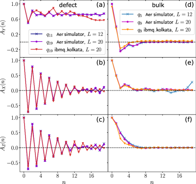
Figure 2: Signature of the zero mode at the defect site for the duality-twisted Floquet-TFIM. The label qiq_{i} denotes the measurement at the iith qubit. Panel (a) shows the nondecaying autocorrelation for σy\sigma_{y} at the defect site r=L1r=L-1, which overlaps with the zero mode. All other autocorrelations both at the twist defect r=L1r=L-1 [panel (b), (c)] and at a bulk site j=1+L/2j=-1+L/2 [panel (d), (e), (f)], far away from the twist defect, decay with stroboscopic time nn. The chosen bulk qubit behaves qualitatively similarly to other bulk qubits. We present data from ibmq_kolkata device for L=20L=20, the longest physical loop of qubits available in the device. There is good qualitative agreement between noiseless simulation and measurements on the noisy quantum device. The noiseless simulations were also performed for a smaller system of 12 qubits. The agreement between the two system sizes L=12,20L=12,20 indicates that we are capturing the behavior in the thermodynamic limit. Date of demonstration at ibmq_kolkata device is 18th April, 2023.

III Detection of the unpaired zero mode in the IBM quantum device

We have chosen the values of the coupling constants to be J=0.75πJ=0.75\pi and g=0.2πg=0.2\pi for all the computations in this paper, although similar results can be obtained for other coupling constants. To create and detect the zero mode in the quantum computer, we apply a quantum circuit that generates the Floquet dynamics by the repeated applications of a circuit block corresponding to the unitary operator in (10). A simple 4-qubit version of this block, corresponding to one Trotter step, is shown in Fig. 1. We compute the autocorrelation (11) for 𝒪=σx,σy\mathcal{O}=\sigma^{x},\sigma^{y}, and σz\sigma^{z} of a 20-qubit system. We perform this calculation on the 27-qubit ibmq_kolkata device with a 20-qubit closed loop. Thus, the device geometry eliminates the need for using swap gates to implement periodic boundary conditions. We used a compound error mitigation method as discussed in Appendix B and described in Refs. Shtanko et al. 2023; Kirmani et al. 2023.

As mentioned above, for a Pauli operator 𝒪\mathcal{O}, we need to create initial states that are eigenstates of the corresponding Pauli operator. Measuring 𝒪=σz\mathcal{O}=\sigma^{z} is the simplest as the input and output in IBM devices are measured in the eigenbasis of σz\sigma^{z} by default. However, both initialization and measurement in a different basis can be implemented through rotation operators Ry(π/2)R_{y}(\pi/2) (Rx(π/2)R_{x}(-\pi/2)) that rotate from the zz to the xx (yy) direction.

In Fig. 2, we present both noiseless simulation and noisy quantum-hardware results for the bulk and defect autocorrelation functions obtained from the partial trace with 20 random basis states. We also show noiseless simulation results from Qiskit Aer simulators for 12-qubit and 20-qubit systems. The simulation results exhibit very small system-size dependence, indicating that the 20-qubit system accurately captures the thermodynamic limit. Furthermore, the results from the ibmq_kolkata device for the 20-qubit system is in good agreement with the noiseless simulations. We observe that the autocorrelation function of 𝒪=σry\mathcal{O}=\sigma^{y}_{r} at the twist defect r=L1r=L-1 does not decay, which overlaps with the emergent Majorana zero mode. In contrast, all other autocorrelators decay to zero in the long time limit. The persistence of the autocorrelation function of the operator corresponding to the unpaired zero mode, during the Floquet dynamics, provides evidence for the dynamical generation of this mode in a digitized quantum device.
IV Unitary translation of twist defect

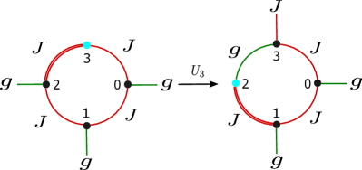
Figure 3: A twist defect that was originally on sites 2 and 3 (left) is moved to sites 1 and 2 (right) by a unitary transformation CZ2,3H2CZ_{2,3}H_{2}. Cyan denotes the site rr at which there is no magnetic field while the double red lines denote a twist interaction σr1zσrx\sigma^{z}_{r-1}\sigma^{x}_{r}. Vertical lines denote a transverse field while solid lines between sites j,j+1j,j+1 denote a σjzσj+1z\sigma^{z}_{j}\sigma^{z}_{j+1} interaction. After the unitary transformation (right), note the Kramers-Wannier duality between sites 2,3 and the rest of the chain where the strength of the transverse field at site 3 is JJ while the exchange interaction between qubits 2 and 3 is gg. The unitary transformation shifts the twist but not the Majorana zero mode which stays localized at site 3. Thus the Majorana zero mode resides at the domain wall across which g,Jg,J exchange roles.
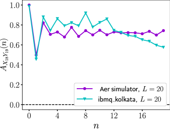
Figure 4: Unpaired Majorana in the ibmq_kolkata device for L=20L=20 after a unitary translation that has moved the twist defect from sites 18,1918,19 to sites 17,1817,18. The Majorana stays localized at site 19 but now has an overlap with the longer Pauli string σ18xσ19y\sigma^{x}_{18}\sigma^{y}_{19}. Date of demonstration is 5th May, 2023.

A hallmark of a topological defect is that it can be moved by local unitary transformations, while leaving the model invariant. Strictly speaking the model is invariant only for g=Jg=J, and in the high frequency limit. Nevertheless, even away from this special case, physical consequences of the topological nature of this defect manifest in the invariance of the position of the zero mode as the twist defect is moved.

A local unitary transformation of the form Ur=CZr1,rHr1U_{r}=CZ_{r-1,r}H_{r-1}, where CZr1,rCZ_{r-1,r} is a controlled-Z gate, and Hr1H_{r-1} is a Hadamard gate, moves the twist-defect from the sites (r1,r)(r-1,r) to sites (r2,r1)(r-2,r-1) Aasen et al. 2016; Mitra et al. 2023. Fig. 3 illustrates this for a 4-qubit system. The unitary UrU_{r} introduces a transverse field at site rr of strength JJ while eliminating the transverse field at site r1r-1. It also changes the terms Jσr2zσr1zJ\sigma_{r-2}^{z}\sigma_{r-1}^{z} and Jσr1zσrxJ\sigma_{r-1}^{z}\sigma_{r}^{x} to Jσr2zσr1xJ\sigma_{r-2}^{z}\sigma_{r-1}^{x} and gσr1zσrzg\sigma_{r-1}^{z}\sigma_{r}^{z}. Thus a Kramers-Wannier duality transformation has been performed on the sites r,r1r,r-1 where the roles of g,Jg,J have been interchanged. Remarkably, the Majorana zero mode stays localized at rr, and now separates two regions of the chain that are related by the Kramers-Wannier duality transformation. Although the Majorana zero mode stays localized at site rr, in the language of Pauli strings, it is a more nonlocal object. In particular, instead of having an overlap with σry\sigma^{y}_{r}, it now has an overlap with σr1xσry\sigma^{x}_{r-1}\sigma^{y}_{r}.

The Majorana zero mode after a translation of the twist defect from (18,19)(18,19) to (17,18)(17,18) for a 20-qubit system is shown in Fig. 4. After one translation, the Majorana is still localized at site r=19r=19, but in the language of Pauli spins, this Majorana zero mode no longer has an overlap with σ19y\sigma^{y}_{19}, but rather with the longer string σ18xσ19y\sigma^{x}_{18}\sigma^{y}_{19}.

V Effects of Interactions

Now we add perturbations to the model (1) through the term

Hxx=Jxjσjxσj+1x.H_{xx}=J_{x}\sum_{j}\sigma_{j}^{x}\sigma_{j+1}^{x}. (12)

In the language of Majorana fermions, the above is a four-fermion and hence interacting term. The Floquet unitary is now given by

Uint=eiHxx/2eiHx/2eiHzx/2eiHzz/2.U_{\text{int}}=e^{-iH_{xx}/2}e^{-iH_{x}/2}e^{-iH_{zx}/2}e^{-iH_{zz}/2}. (13)

Note that HxxH_{xx} not only breaks integrability, but it also does not commmute with the discrete symmetry Ωr\Omega_{r} due to the σr±1xσrx\sigma^{x}_{r\pm 1}\sigma^{x}_{r} terms. We repeat the same quantum simulation for the interacting model with the defect location at site r=L1r=L-1. We find that the σry\sigma^{y}_{r}-correlator at the defect remains constant, while all other correlators decay with time as shown in Fig. 5. We observe a similar behavior to the noninteracting case shown in Fig. 2 for both bulk and defect autocorrelation functions, within the studied number of Floquet cycles.

Figure 5: Signature of the Majorana zero mode at the defect site for duality-twisted interacting Floquet-TFIM. Panel (a) shows the nondecaying autocorrelation for σy\sigma_{y} at the defect site r=L1r=L-1, which overlaps with the zero mode. All other autocorrelations both at the twist defect r=L1r=L-1 [panel (b), (c)] and at a bulk site j=1+L/2j=-1+L/2 [panel (d), (e), (f)], far away from the twist defect, decay with time. The chosen bulk qubit behaves qualitatively similarly to other bulk qubits. We present data from ibmq_kolkata device for L=20L=20, the longest physical loop of qubits available in the device. There is good qualitative agreement between noiseless simulations and measurements on the noisy quantum device. The noiseless simulations were also performed for a smaller system of 12 qubits. The agreement between the two system sizes L=12,20L=12,20 indicates that we capture the behavior in the thermodynamic limit for these times. At longer times, we expect a stronger LL dependence discussed in the main text. The label qiq_{i} indicates measurement of the iith qubit. Date of demonstrations is 22nd April, 2023.

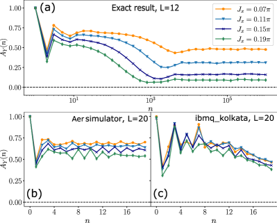
We note, however, that the long time dynamics of the σry\sigma^{y}_{r}-correlator at the defect is not captured in this figure as we can run the Floquet dynamics in the device only for about 20 Floquet cycles before noise takes over. We show the theoretical behavior of the Majorana zero mode by performing exact diagonalization for long times in Fig. 6(a). After the initial decay to the first plataeu, the Majorana mode decays to a second plateau. The plateau heights decrease with increasing interactions JxJ_{x}. We capture only the initial portions of this behavior in the quantum device [see Fig. 6(b) and (c)], i.,e the decay to the first plateau. While the first plateau height is not LL dependent (as seen in the simulations in Fig. 5), we expect that the second plateau height is LL dependent, where as LL\rightarrow\infty, the plateau height decreases to zero. This is because, there is no exact zero mode when we break integrability, with the zero mode decaying via scattering with bulk excitations Yeh et al. 2023. However, a finite size system blocks these scattering processes leading to a partial decay, and hence a plateau height which is inversely related to system size Mitra et al. 2023. A second important observation is that while the interactions now couple the two Z2Z_{2} sectors, yet the zero modes in the two sectors do not efficiently couple to each other as is evident by the appearance of the second plateau, which persists at long times. This is again a finite system size effect.

Figure 6: Stability of the Majorana zero mode to integrability- and symmetry-breaking perturbations in a finite system. The autocorrelation function of σry\sigma^{y}_{r} at the defect r=L1r=L-1, for different values of the perturbation JxJ_{x}, are presented. Panel (a) shows the numerical results for system size L=12L=12 up to large Floquet time steps. After the initial transient corresponding to the appearance of a first plateau, the autocorrelation stabilizes at a second plateau. This is a finite size effect where the height of the second plateau vanishes as LL\to\infty Mitra et al. 2023. While we are not able to access this second plateau in the long-time limit in the ibmq_kolkata device due to noise, panels (b) and (c) show results from the IBM simulator and the ibmq_kolkata device, respectively, for intermediate timescales. At these timescales, the formation of the first plateau is clearly visible. Date of demonstrations is 27th April, 2023.

VI Conclusions

In this paper, we investigated the physics of the duality twist defect and the corresponding emergent zero mode in a periodically driven TFIM loop of 20 qubits on the IBM superconducting quantum device. The interplay of topological effects and symmetries can lead to novel phenomena. The zero mode generated by a duality twist in a TFIM chain commutes with the Z2Z_{2} charge of the model and thus, theoretically, has an infinite lifetime in finite systems Tan et al. 2024 (in contrast to edge states with open boundary conditions that are vulnerable to exponential hybridization). Using efficient random sampling, we obtained an accurate approximation to various autocorrelation functions and provided evidence, on the quantum computer, for the emergence of the unpaired zero mode bound to the duality twist defect. Furthermore, we explored the effects of moving the duality twist defect with unitary gates, and the effect of integrability- and symmetry-breaking perturbations. This work opens a new avenue for physically creating and investigating topological defects in quantum systems, and exploring their ramifications on nonequilibrium dynamics, a topic poorly understood theoretically.

Future improvements in hardware quality and error mitigation may allow accessing longer evolution times with deeper circuits, providing access to the long-time plateaus of persistent autocorrelation functions in the presence of interactions. Exciting directions of future research include implementing topological defects on the quantum computer, not only in ZnZ_{n} spin chains Aasen et al. 2020, but also in two-dimensional Floquet codes Hastings and Haah 2021.

Acknowledgements.
We thank Oles Shtanko for helpful comments and discussions. We acknowledge the use of IBM Quantum services. We also thank the Brookhaven National Laboratory for providing access to IBM devices. This work was supported by the US National Science Foundation under Grants NSF DMR-2018358 (AM) and DMR-1945395 (AR and SS), and in part by the US National Science Foundation under Grant No. NSF PHY-1748958 (AR and AM).

Appendix A Convergence of the partial trace

In this section, we provide evidence for the accurate approximation of the autocorrelation functions (based on the full trace) by a partial trace with a small number of random basis states. In Fig. 7, we show the expectation value with a single random state, and the partial trace with 20 random initial states, and we compare them with the full trace calculated with all 2122^{12} basis states for a system of size L=12L=12. We have calculated these quantities for all three Pauli operators. Even a single expectation value is relatively close to the exact (full trace) autocorrelation function, for both bulk and defect sites, due to the little variation between these expectation values. The results of the partial trace with 20 random states are in excellent agreement with the full trace, supporting the use of the partial trace to approximate the autocorrelation functions.

Figure 7: Autocorrelation functions from computing the partial trace in a classical computer for different sample sizes of random initial states, for system size L=12L=12. The left panels [panel (a), (b), (c)] show the autocorrelation functions at the site of twist defect r=L1r=L-1, while the right panels [panel (d), (e), (f)] are for a site far away from it, j=1+L/2j=-1+L/2.

All expectation values are the same, and correspond to the YY autocorrelation function at the defect site. Thus for this particular observable, the trace is independent of the number of basis states used.

Appendix B Error Mitigation

We employ a composite error mitigation strategy combining error suppression and mitigation techniques Ferris et al. 2022. Noisy bitstrings resulting from each shot are first mitigated by correcting readout errors using the method of Ref. Nation et al. 2021, which utilizes calibration circuits scaling linearly with the number of qubits. Finally, zero-noise extrapolation is applied by extrapolating measured probabilities to the zero-noise value Li and Benjamin 2017; Temme et al. 2017. This is achieved by performing measurements with 8,000 shots at noise factors of 1 (applying the original circuit) and 3 (evolving the system forward by the original circuit, backward by appending the inverse of the original circuit, and finally forward again by reapplying the original circuit Rivero et al. 2022). A line through 1 and 3 on the horizontal axis yield the zero-noise extrapolated value at the intercept with the vertical axis.

Appendix C Layout of the computing device and its characteristics

The layout of ibmq_kolkata device is shown in Fig. 8.

Refer to caption
Figure 8: Qubit layout of ibmq_kolkata device

We use the 20 qubit loop consisting of qubits 1, 2, 3, 5, 8, 11, 14, 16, 19, 22, 25, 24, 23, 21, 18, 15, 12, 10, 7, and 4 for our demonstrations. We choose the link between qubit 12 and qubit 15 to place the twist defect. The readout length for all these runs was 640ns640ns. P01P_{01} (P10P_{10} )is the probability that measuring a qubit gives 0 (1) immediately after preparing it in state 1 (0). The readout error is indicated as RE, and the frequency ff and the anharmonicity aa are both in GHz. The calibration data from 18th April, 2023 for the used qubits are given in Table 1, and the error map is shown in Fig. 9. The calibration data from 22nd April, 2023 for the used qubits are given in Table 2, and the error map is shown in Fig. 10. The calibration data from 27th April, 2023 for the used qubits are given in Table 3, and the error map is shown in Fig. 11. The calibration data from 5th May, 2023 for the used qubits are given in Table 4, and the error map is shown in Fig. 12. The error maps are generated using Qiskit’s visualization library.

Qubit T1(μ\mus) T2(μ\mus) ff aa RE P01P_{01} P10P_{10}
1 81.37 181.74 4.99 0.34-0.34 0.0087 0.0112 0.0062
2 72.9 52.5 5.11 0.34-0.34 0.0155 0.022 0.009
3 126.2 165.5 4.87 0.35-0.35 0.013 0.0122 0.0138
5 128.1 29.5 5.11 0.342-0.342 0.0325 0.0344 0.0306
8 135.2 60.4 4.93 0.345-0.345 0.0427 0.0292 0.0562
11 132.8 43.6 4.87 0.373-0.373 0.1247 0.1182 0.1312
14 58.82 70.08 5.12 0.343-0.343 0.06 0.0216 0.0984
16 78.78 116.12 5.22 0.34-0.34 0.0092 0.0078 0.0106
19 86.69 32.28 5.002 0.345-0.345 0.0383 0.0208 0.0558
22 108.02 39.49 5.127 0.343-0.343 0.0369 0.0352 0.0386
25 253.27 83.23 4.92 0.347-0.347 0.0098 0.0124 0.0072
24 120.36 86.38 5.004 0.346-0.346 0.0092 0.0096 0.0088
23 153.89 48.45 5.138 0.343-0.343 0.0135 0.0214 0.0056
21 83.88 17.18 5.274 0.341-0.341 0.0073 0.0108 0.0038
18 163.04 104.59 5.097 0.344-0.344 0.0102 0.0126 0.0078
15 175.32 207.31 5.041 0.344-0.344 0.0053 0.007 0.0036
12 148.89 137.72 4.96 0.346-0.346 0.0088 0.01 0.0076
10 113.57 44.2 5.178 0.342-0.342 0.0151 0.014 0.0162
7 164.47 33.13 5.031 0.346-0.346 0.0223 0.0208 0.0238
4 87.74 87.38 5.224 0.341-0.341 0.0214 0.0224 0.0204
Table 1: Calibration data for the qubits used for demonstrations on 18th April, 2023.
Qubit T1(μ\mus) T2(μ\mus) ff aa RE P01P_{01} P10P_{10}
1 17.686 106.2 4.99 0.345-0.345 0.0203 0.0272 0.0134
2 42.29 37.02 5.117 0.343-0.343 0.0516 0.078 0.0252
3 143.82 188.71 4.866 0.346-0.346 0.0102 0.0114 0.009
5 103.63 30.41 5.113 0.342-0.342 0.032 0.0332 0.0308
8 163.56 50.83 4.928 0.345-0.345 0.0451 0.032 0.0582
11 139.18 39.37 4.868 0.373-0.373 0.1176 0.1116 0.1236
14 128.15 67.17 5.117 0.343-0.343 0.0629 0.0246 0.1012
16 96.47 92.36 5.222 0.34-0.34 0.0111 0.0084 0.0138
19 112.28 26.24 5.002 0.345-0.345 0.0776 0.0316 0.1236
22 115.85 38.87 5.127 0.343-0.343 0.0411 0.0383 0.0438
25 167.11 81.57 4.92 0.347-0.347 0.0088 0.0122 0.0054
24 122.28 83.58 5.004 0.346-0.346 0.0083 0.0108 0.0058
23 127.04 42.31 5.138 0.343-0.343 0.0143 0.026 0.0026
21 69.81 16.35 5.274 0.341-0.341 0.0069 0.0078 0.006
18 70.17 105.99 5.097 0.344-0.344 0.0087 0.0086 0.0088
15 157.17 192.35 5.041 0.344-0.344 0.0061 0.008 0.0042
12 144.32 174.84 4.961 0.346-0.346 0.0075 0.0092 0.0058
10 88.61 35.82 5.178 0.342-0.342 0.0106 0.0144 0.0068
7 68.69 34.22 5.031 0.345-0.345 0.0242 0.0254 0.023
4 108.36 66.99 5.224 0.341-0.341 0.0216 0.0202 0.023
Table 2: Calibration data for the qubits used for demonstrations on 22nd April, 2023.
Qubit T1(μ\mus) T2(μ\mus) ff aa RE P01P_{01} P10P_{10}
1 249.53 176.45 4.991 0.345-0.345 0.0112 0.012 0.0098
2 10.43 44.90 5.117 0.343-0.343 0.0149 0.019 0.0108
3 75.96 136.94 4.866 0.346-0.346 0.0143 0.0158 0.0128
5 133.18 31.47 5.113 0.342-0.342 0.0323 0.0324 0.0322
8 125.48 49.20 4.928 0.345-0.345 0.0342 0.0328 0.0356
11 149.91 41.34 4.868 0.373-0.373 0.0944 0.0956 0.0932
14 165.77 204.37 5.117 0.343-0.343 0.0657 0.0244 0.107
16 106.17 84.22 5.222 0.34-0.34 0.009 0.007 0.011
19 54.53 23.02 5.002 0.345-0.345 0.0387 0.0252 0.0522
22 138.54 34.42 5.127 0.343-0.343 0.0372 0.037 0.0374
25 222.14 120.88 4.921 0.347-0.347 0.0109 0.0156 0.0062
24 93.44 106.77 5.005 0.346-0.346 0.0094 0.0104 0.0084
23 135.32 52.53 5.138 0.343-0.343 0.0035 0.005 0.002
21 124.1 18.48 5.274 0.341-0.341 0.0047 0.0052 0.0042
18 117.51 148.1 5.097 0.344-0.344 0.0094 0.0112 0.0076
15 129.05 224.34 5.041 0.344-0.344 0.0067 0.0072 0.0064
12 205.67 225.1 4.961 0.346-0.346 0.0075 0.0084 0.0066
10 85.16 38.17 5.178 0.342-0.342 0.00870.0087 0.0094 0.008
7 170.34 45.36 5.031 0.346-0.346 0.0261 0.0202 0.032
4 122.95 100.49 5.224 0.341-0.341 0.0196 0.021 0.0182
Table 3: Calibration data for the qubits used for demonstrations on 27th April, 2023.
Qubit T1(μ\mus) T2(μ\mus) ff aa RE P01P_{01} P10P_{10}
1 176.13 214.04 4.991 0.345-0.345 0.0099 0.0146 0.0052
2 10.9 44.9 5.113 0.343-0.343 0.0149 0.019 0.0108
3 96.79 195.85 4.866 0.346-0.346 0.0128 0.0118 0.0138
5 88.86 29.91 5.113 0.342-0.342 0.0348 0.0348 0.0348
8 129.58 52.25 4.928 0.345-0.345 0.0277 0.0248 0.0306
11 133.31 37.53 4.868 0.373-0.373 0.123 0.1296 0.1164
14 156.54 169.92 5.117 0.343-0.343 0.0660.066 0.022 0.11
16 113.15 103.99 5.222 0.3402-0.3402 0.0079 0.008 0.0078
19 105.14 28.67 5.002 0.345-0.345 0.0699 0.025 0.1148
22 116.19 32.82 5.127 0.343-0.343 0.0382 0.0344 0.042
25 194.42 73.42 4.921 0.347-0.347 0.0056 0.0072 0.004
24 107.53 107.29 5.005 0.346-0.346 0.0097 0.0106 0.0088
23 115.88 50.13 5.138 0.343-0.343 0.0044 0.0058 0.003
21 94.18 19.34 5.274 0.341-0.341 0.0062 0.0062 0.0062
18 145.87 125.4 5.097 0.344-0.344 0.0092 0.0104 0.008
15 91.18 153.23 5.041 0.344-0.344 0.0066 0.0084 0.0048
12 175.97 188.79 4.961 0.346-0.346 0.0078 0.009 0.0066
10 120.79 38.97 5.178 0.342-0.342 0.015 0.0092 0.0208
7 144.69 54.6 5.031 0.346-0.346 0.0239 0.0292 0.0186
4 145.79 139.71 5.225 0.341-0.341 0.02320.0232 0.0248 0.0216
Table 4: Calibration data for the qubits used for demonstrations on 5th May, 2023.
Refer to caption
Figure 9: Error map for qubits and couplings of imbq_kolkata device from 18th April, 2023.
Refer to caption
Figure 10: Error map for qubits and couplings of imbq_kolkata device from 22nd April, 2023
Refer to caption
Figure 11: Error map for qubits and couplings of imbq_kolkata device from 27th April, 2023
Refer to caption
Figure 12: Error map for qubits and couplings of imbq_kolkata device from 5th May, 2023

References

  • Cobanera et al. (2011) E. Cobanera, G. Ortiz, and Z. Nussinov, The bond-algebraic approach to dualities, Adv. Phys. 60, 679 (2011).
  • Seiberg et al. (2016) N. Seiberg, T. Senthil, C. Wang, and E. Witten, A duality web in 2+1 dimensions and condensed matter physics, Ann. Phys. 374, 395 (2016).
  • Somoza et al. (2021) A. M. Somoza, P. Serna, and A. Nahum, Self-dual criticality in three-dimensional z2z_{2} gauge theory with matter, Phys. Rev. X 11, 041008 (2021).
  • Lootens et al. (2021) L. Lootens, C. Delcamp, G. Ortiz, and F. Verstraete, Dualities in one-dimensional quantum lattice models: symmetric hamiltonians and matrix product operator intertwiners, arXiv:2112.09091 (2021).
  • Verlinde (1988) E. Verlinde, Fusion rules and modular transformations in 2d conformal field theory, Nucl. Phys. B 300, 360 (1988).
  • Bhardwaj et al. (2023) L. Bhardwaj, L. E. Bottini, S. Schäfer-Nameki, and A. Tiwari, Non-invertible higher-categorical symmetries, SciPost Phys. 14, 007 (2023).
  • Aasen et al. (2016) D. Aasen, R. S. K. Mong, and P. Fendley, Topological defects on the lattice: I. the ising model, J. Phys. A: Math. Theor. 49, 354001 (2016).
  • Thorngren and Wang (2019) R. Thorngren and Y. Wang, Fusion category symmetry i: Anomaly in-flow and gapped phases, arXiv:1912.02817 (2019).
  • Aasen et al. (2020) D. Aasen, P. Fendley, and R. S. Mong, Topological defects on the lattice: dualities and degeneracies, arXiv:2008.08598 (2020).
  • Kong et al. (2020) L. Kong, T. Lan, X.-G. Wen, Z.-H. Zhang, and H. Zheng, Algebraic higher symmetry and categorical symmetry: A holographic and entanglement view of symmetry, Phys. Rev. Res. 2, 043086 (2020).
  • McGreevy (2022) J. McGreevy, Generalized Symmetries in Condensed Matter, arXiv:2204.03045 (2022).
  • Gaiotto et al. (2015) D. Gaiotto, A. Kapustin, N. Seiberg, and B. Willett, Generalized global symmetries, J. High Energy Phys. 2015 (2), 172.
  • Gaiotto et al. (2021) D. Gaiotto, J. H. Lee, and J. Wu, Integrable kondo problems, J. High Energy Phys. 2021 (4).
  • Cheng and Seiberg (2023) M. Cheng and N. Seiberg, Lieb-schultz-mattis, luttinger, and ’t hooft – anomaly matching in lattice systems, arXiv:2211.12543 (2023).
  • Eck and Fendley (2023) L. Eck and P. Fendley, From the xxz chain to the integrable rydberg-blockade ladder via non-invertible duality defects, arXiv:2302.14081 (2023).
  • Preskill (2018) J. Preskill, Quantum Computing in the NISQ era and beyond, Quantum 2, 79 (2018).
  • Kramers and Wannier (1941) H. A. Kramers and G. H. Wannier, Statistics of the two-dimensional ferromagnet. Part 1., Phys. Rev. 60, 252 (1941).
  • Tan et al. (2024) M. T. Tan, Y. Wang, and A. Mitra, Topological defects in floquet circuits, SciPost 16, 075 (2024).
  • Cardy (1989) J. L. Cardy, Boundary conditions, fusion rules and the verlinde formula, Nucl. Phys. B 324, 581 (1989).
  • Schutz (1993) G. Schutz, ’duality twisted’ boundary conditions in n-state potts models, Journal of Physics A: Mathematical and General 26, 4555 (1993).
  • Oshikawa and Affleck (1997) M. Oshikawa and I. Affleck, Boundary conformal field theory approach to the critical two-dimensional ising model with a defect line, Nuclear Physics B 495, 533 (1997).
  • Petkova and Zuber (2001) V. B. Petkova and J. B. Zuber, Generalized twisted partition functions, Phys. Lett. B 504, 157 (2001).
  • Grimm (2002) U. Grimm, Spectrum of a duality twisted Ising quantum chain, J. Phys. A 35, L25 (2002), arXiv:hep-th/0111157 .
  • Fröhlich et al. (2004) J. Fröhlich, J. Fuchs, I. Runkel, and C. Schweigert, Kramers-wannier duality from conformal defects, Phys. Rev. Lett. 93, 070601 (2004).
  • Chang et al. (2019) C.-M. Chang, Y.-H. Lin, S.-H. Shao, Y. Wang, and X. Yin, Topological defect lines and renormalization group flows in two dimensions, J. High Energy Phys. 01, 026.
  • Kitaev (2001) A. Y. Kitaev, Unpaired majorana fermions in quantum wires, Phys.-Usp. 44 (2001).
  • Fendley (2016) P. Fendley, Strong zero modes and eigenstate phase transitions in the xyz/interacting majorana chain, Journal of Physics A: Mathematical and Theoretical 49, 30LT01 (2016).
  • Thakurathi et al. (2013) M. Thakurathi, A. A. Patel, D. Sen, and A. Dutta, Floquet generation of majorana end modes and topological invariants, Phys. Rev. B 88, 155133 (2013).
  • Yates et al. (2019) D. J. Yates, F. H. L. Essler, and A. Mitra, Almost strong (0,π0,\pi) edge modes in clean interacting one-dimensional floquet systems, Phys. Rev. B 99, 205419 (2019).
  • Mitra et al. (2023) A. Mitra, H.-C. Yeh, F. Yan, and A. Rosch, Nonintegrable floquet ising model with duality twisted boundary conditions, Phys. Rev. B 107, 245416 (2023).
  • Rahmani et al. (2020) A. Rahmani, K. J. Sung, H. Putterman, P. Roushan, P. Ghaemi, and Z. Jiang, Creating and manipulating a laughlin-type ν=1/3\nu=1/3 fractional quantum hall state on a quantum computer with linear depth circuits, PRX Quantum 1, 020309 (2020).
  • Satzinger et al (2021) K. Satzinger et al, Realizing topologically ordered states on a quantum processor, Science 374, 1237 (2021).
  • Stenger et al. (2021) J. P. T. Stenger, N. T. Bronn, D. J. Egger, and D. Pekker, Simulating the dynamics of braiding of majorana zero modes using an ibm quantum computer, Phys. Rev. Res. 3, 033171 (2021).
  • Liu et al. (2022) Y.-J. Liu, K. Shtengel, A. Smith, and F. Pollmann, Methods for simulating string-net states and anyons on a digital quantum computer, PRX Quantum 3, 040315 (2022).
  • Kirmani et al. (2022) A. Kirmani, K. Bull, C.-Y. Hou, V. Saravanan, S. M. Saeed, Z. Papić, A. Rahmani, and P. Ghaemi, Probing geometric excitations of fractional quantum hall states on quantum computers, Phys. Rev. Lett. 129, 056801 (2022).
  • Andersen et al (2023) T. I. Andersen et al, Non-abelian braiding of graph vertices in a superconducting processor, Nature 618, 264 (2023).
  • Harle et al. (2023) N. Harle, O. Shtanko, and R. Movassagh, Observing and braiding topological majorana modes on programmable quantum simulators, Nat. Comm. 14, 2286 (2023).
  • Kirmani et al. (2023) A. Kirmani, D. S. Wang, P. Ghaemi, and A. Rahmani, Braiding fractional quantum hall quasiholes on a superconducting quantum processor, arXiv:2303.04806 (2023).
  • Mi and et al (2022) X. Mi and et al, Noise-resilient edge modes on a chain of superconducting qubits, Science 378, 785 (2022).
  • Sinha et al. (2024) M. Sinha, F. Yan, L. Grans-Samuelsson, A. Roy, and H. Saleur, Lattice realizations of topological defects in the critical (1+1)-d three-state Potts model, JHEP 07, 225, arXiv:2310.19703 [hep-th] .
  • Seiberg et al. (2024) N. Seiberg, S. Seifnashri, and S.-H. Shao, Non-invertible symmetries and LSM-type constraints on a tensor product Hilbert space, SciPost Phys. 16, 154 (2024), arXiv:2401.12281 [cond-mat.str-el] .
  • Parayil Mana et al. (2024) A. Parayil Mana, Y. Li, H. Sukeno, and T.-C. Wei, Kennedy-Tasaki transformation and noninvertible symmetry in lattice models beyond one dimension, Phys. Rev. B 109, 245129 (2024), arXiv:2402.09520 [cond-mat.str-el] .
  • Chatterjee et al. (2024) A. Chatterjee, Ömer M. Aksoy, and X.-G. Wen, Quantum phases and transitions in spin chains with non-invertible symmetries, SciPost Phys. 17, 115 (2024).
  • Lu et al. (2024) D.-C. Lu, Z. Sun, and Y.-Z. You, Realizing triality and pp-ality by lattice twisted gauging in (1+1)d quantum spin systems, arxiv.2405.14939 (2024).
  • Cao et al. (2024) W. Cao, L. Li, and M. Yamazaki, Generating lattice non-invertible symmetries, SciPost Phys. 17, 104 (2024).
  • Yan et al. (2024) F. Yan, R. Konik, and A. Mitra, Duality defect in a deformed transverse-field ising model, arXiv:2410.17317 (2024).
  • Hauru et al. (2016) M. Hauru, G. Evenbly, W. W. Ho, D. Gaiotto, and G. Vidal, Topological conformal defects with tensor networks, Phys. Rev. B 94, 115125 (2016).
  • Rogerson et al. (2022) D. Rogerson, F. Pollmann, and A. Roy, Entanglement entropy and negativity in the ising model with defects, Journal of High Energy Physics 2022, 10.1007/jhep06(2022)165 (2022).
  • Roy and Saleur (2022) A. Roy and H. Saleur, Entanglement entropy in the ising model with topological defects, Phys. Rev. Lett. 128, 090603 (2022).
  • Shtanko et al. (2023) O. Shtanko, D. S. Wang, H. Zhang, N. Harle, A. Seif, R. Movassagh, and Z. Minev, Uncovering local integrability in quantum many-body dynamics, arXiv:2307.07552 (2023).
  • Yeh et al. (2023) H.-C. Yeh, A. Rosch, and A. Mitra, Decay rates of almost strong modes in floquet spin chains beyond fermi’s golden rule, Phys. Rev. B 108, 075112 (2023).
  • Hastings and Haah (2021) M. B. Hastings and J. Haah, Dynamically Generated Logical Qubits, Quantum 5, 564 (2021).

  • Ferris et al. (2022) K. J. Ferris, A. J. Rasmusson, N. T. Bronn, and O. Lanes, Quantum Simulation on Noisy Superconducting Quantum Computers, arXiv:2209.02795[quant-ph] (2022).
  • Nation et al. (2021) P. D. Nation, H. Kang, N. Sundaresan, and J. M. Gambetta, Scalable mitigation of measurement errors on quantum computers, PRX Quantum 2, 040326 (2021).
  • Li and Benjamin (2017) Y. Li and S. C. Benjamin, Efficient variational quantum simulator incorporating active error minimization, Phys. Rev. X 7, 021050 (2017).
  • Temme et al. (2017) K. Temme, S. Bravyi, and J. M. Gambetta, Error mitigation for short-depth quantum circuits, Phys. Rev. Lett. 119, 180509 (2017).
  • Rivero et al. (2022) P. Rivero, F. Metz, A. Hasan, A. M. Brańczyk, and C. Johnson, Zero noise extrapolation prototype, https://github.com/qiskit-community/prototype-zne (2022).