Intensity-free Integral-based Learning of Marked Temporal Point Processes

Abstract

In the marked temporal point processes (MTPP), a core problem is to parameterize the conditional joint PDF (probability distribution function) $p^{*}(m,t)$ for inter-event time $t$ and mark $m$, conditioned on the history. The majority of existing studies predefine intensity functions. Their utility is challenged by specifying the intensity function’s proper form, which is critical to balance expressiveness and processing efficiency. Recently, there are studies moving away from predefining the intensity function – one models $p^{*}(t)$ and $p^{*}(m)$ separately, while the other focuses on temporal point processes (TPPs), which do not consider marks. This study aims to develop high-fidelity $p^{*}(m,t)$ for discrete events where the event marks are either categorical or numeric in a multi-dimensional continuous space. We propose a solution framework IFIB (Intensity-free Integral-based process) that models conditional joint PDF $p^{*}(m,t)$ directly without intensity functions. It remarkably simplifies the process to compel the essential mathematical restrictions. We show the desired properties of IFIB and the superior experimental results of IFIB on real-world and synthetic datasets. The code is available at https://github.com/StepinSilence/IFIB.

1 Introduction

Events have been generated continuously in human activities or observed from natural phenomena. The events can be financial transactions, social media user activities, Web page visits by users, patient visits to clinics, earthquake occurrences in seismology, neural spike trains in neuroscience, the extreme temperature in the weather forecast, and the observations of rare birds in ecology. Temporal point processes (TPP) are generative models of variable-length point sequences which represent the arrival times of events. TPPs are built upon rich theoretical foundations, with early work dating back to many decades ago, where they were used to model the arrival of insurance claims and telephone traffic Shchur et al. [2020], till now widely applied in social network analysis, neural logic inference, and biological activity modeling.

The marked TPP (MTPP) concerns the scenarios where each event comes with an arrival time as well as a mark. The mark can be categorical such as the magnitude of earthquakes, mild/moderate/critical symptoms of patients visiting an emergency, sell/buy in financial transactions, or numeric such as temperature in the weather forecast, the longitude and latitude of observations in ecology. As often encountered in practice, the marked TPP has attracted much attention from the research community Du et al. [2016], Mei and Eisner [2017], Guo et al. [2018], Enguehard et al. [2020], Zuo et al. [2020], Zhang et al. [2020], Mei et al. [2020], Shchur et al. [2020], Charpentier et al. [2019], Chen et al. [2020]. Most studies assume the events in sequence are correlated so that the marked TPPs are conditioned on history, i.e., the events that occurred so far.

A core problem of marked TPP is to parameterize the conditional joint PDF $p^{*}(m,t)$ for inter-event time $t$ and mark $m$, conditioned on the history $\mathcal{H}_{t_{l}}$ Shchur et al. [2020]. Many applications regarding the time and mark of the next event depend on $p^{*}(m,t)$. The widely studied one is to predict when the next event will occur and, given the time, which mark the next event is Du et al. [2016], Mei and Eisner [2017], Guo et al. [2018], Enguehard et al. [2020], Zuo et al. [2020], Zhang et al. [2020], Mei et al. [2020], Shchur et al. [2020]. Moreover, for each mark, if its probability to be the next event is non-zero, it is interesting to predict when the next event will occur conditioned on the fact that the next event is the mark. Besides that, one can report the evolution of probabilities for different marks to be the next event over time Charpentier et al. [2019].

The majority of existing studies model $p^{*}(m,t)$ by defining the intensity function Enguehard et al. [2020], Daley and Vere-Jones [2003], Mei and Eisner [2017], Zuo et al. [2020]. They suffer from the expressiveness issue if the intensity function is simple or encounter the computationally-expensive intensity integral problem if complex. One recent study moves away from specifying the form of the intensity function by exploring a neural network Omi et al. [2019]. The solution known as FullyNN is designed for TPP rather than marked TPP, which does not consider event marks. In another recent study, an intensity-free solution has been proposed Shchur et al. [2020] where $p^{*}(m)$ and $p^{*}(t)$ are modeled separately, still, it does not directly address the challenge of modeling $p^{*}(m,t)$. The intensity function of TPP where marks are locations in a continuous spatial space has been studied recently Chen et al. [2020].

This study aims to develop high-fidelity $p^{*}(m,t)$ for discrete events where the event marks are either categorical or numeric. If numeric, the event mark is represented as a vector in a multi-dimensional continuous space. We propose a solution framework IFIB (Intensity-free Integral-based process) that models conditional joint PDF $p^{*}(m,t)$ directly without intensity functions. It remarkably simplifies the process to compel the essential mathematical restrictions. IFIB has two variants, IFIB-C and IFIB-N, where IFIB-C is IFIB for categorical marks, and IFIB-N is IFIB for numeric marks. To the best of our knowledge, IFIB is the first model of its kind. The superiority of IFIB has been verified by experiments on real-world and synthetic datasets in different applications. The source code and data used in this study will be available upon acceptance.

2 Preliminaries

The marked TPP is a random process whose embodiment is a sequence of discrete events, $\mathcal{S}=\{(\mathtt{m}_{i},t_{i})\}_{i=1}^{l}$, where $i\in\mathbb{Z}^{+}$ is the sequence order, $t_{i}\in\mathbb{R}^{+}$ is the time when the $i$th event occurs, $\mathtt{m}_{i}$ is the mark of the $i$th event, and $t_{i}<t_{j}$ if $i<j$. This paper considers the simple marked TPP, which allows at most one event at every time. The time of the most recent event is $t_{l}$, and the current time is $t>t_{l}$. The time interval between two adjacent events is inter-event time. We assume that the occurrence of an event with a particular mark at a particular time may be triggered by what happened in the past. Let $\mathcal{H}_{t_{l}}$ be the history up to (including) the most recent event, and $\mathcal{H}_{t-}$ be the history up to (excluding) the current time Rasmussen [2018]. In different application scenarios, the mark $\mathtt{m}$ can be either categorical or numeric. If categorical, the mark $\mathtt{m}$ is denoted as $m$ which is in a finite set of labels $\mathrm{M}=\{k_{1},k_{2},\cdots,k_{|\mathrm{M}|}\}$. If numeric, the mark $\mathtt{m}$ is denoted as $\mathbf{m}$ which is a vector $(d_{1},\cdots,d_{n})$ in $\mathbf{M}$, a $n$-dimensional continuous space where the value range is $[a_{i},b_{i}]$ for dimension $i$.

Categorical Mark when $\mathtt{m}$ is the categorical mark, the conditional intensity function of the marked TPP can be defined:

$$\lambda^{*}(m=k_{i},t)=\lambda(m=k_{i},t|\mathcal{H}_{t-})=\lim_{\Delta t\rightarrow 0}\frac{P(m=k_{i},t\in[t,t+\Delta t)|\mathcal{H}_{t-})}{\Delta t}.$$ (1)

With $\lambda^{*}(m,t)$, the conditional joint PDF of the next event can be defined:

$$p^{*}(m,t)=p(m,t|\mathcal{H}_{t_{l}})=\lambda^{*}(m,t)F^{*}(t)=\lambda^{*}(m,t)\exp({-\int_{t_{l}}^{t}{\sum_{n\in\mathrm{M}}\lambda^{*}(n,t)d\tau}}).$$ (2)

where $F^{*}(t)$ is the conditional probability that no event has ever happened up to time $t$ since $t_{l}$.

Numeric Mark When $\mathtt{m}$ is the numeric mark, the conditional intensity function of the marked TPP can be defined:

$$\lambda^{*}(\mathbf{m},t)=\lambda(\mathbf{m},t|\mathcal{H}_{t-})=\lim_{\Delta t\rightarrow 0,|\mathcal{C}(\mathbf{m})|\rightarrow 0}\frac{P(\mathbf{m}\in\mathcal{C}(\mathbf{m}),t\in[t,t+\Delta t)|\mathcal{H}_{t-})}{\Delta t|\mathcal{C}(\mathbf{m})|}.$$ (3)

where $\mathcal{C}(\mathbf{m})$ refers to a small hypercube in $\mathbf{M}$ that centers at $\mathbf{m}$ and $|\mathcal{C}(\mathbf{m})|$ is the volume of $\mathcal{C}(\mathbf{m})$. With $\lambda^{*}(\mathbf{m},t)$, the conditional joint PDF of the next event can be defined:

$$p^{*}(\mathbf{m},t)=p(\mathbf{m},t|\mathcal{H}_{t_{l}})=\lambda^{*}(\mathbf{m},t)F^{*}(t)=\lambda^{*}(\mathbf{m},t)\exp({-\int_{t_{l}}^{t}{\int_{\mathbf{m}\in\mathbf{M}}\lambda^{*}(\mathbf{m},t)d\tau}d\mathbf{m}}).$$ (4)

The detailed elaboration about how we obtain Equation 2 from Equation 1 and obtain Equation 3 from Equation 4 is in Appendix A. In this study, our task is to model the conditional joint PDF $p^{*}(\mathtt{m},t)$ where $\mathtt{m}$ is either categorical or numeric.

The simplest form of TPP is the homogeneous Poisson process whose intensity merely contains a positive number $\lambda^{*}(t)=c$. It is widely used in the thinning algorithm Ogata [1981] for creating synthetic datasets based on almost any predefined intensity functions. Another example is the Hawkes process HAWKES [1971], belonging to the self-exciting point process family. Its conditional intensity function is in the form of $\lambda^{*}(t)=\mu+\sum_{i:t_{i}<t}{\kappa(t,t_{i})}$, $\kappa(t,t_{i})>0$, showing that every event excites the intensity function before it falls. Because it meets the real-world intuition that people’s interest always drastically drops as time passes, the Hawkes process is a widely used prior distribution in various TPP models Cao et al. [2017], Mei and Eisner [2017], Salehi et al. [2019].

3 Related Work

Most studies specify a separate intensity function for each categorical mark $k$ (i.e., the probability that the event of a particular mark will occur at any specific future time) based on which density function $p^{*}(m,t)$ can be formulated Enguehard et al. [2020], Daley and Vere-Jones [2003], Mei and Eisner [2017], Zuo et al. [2020], Du et al. [2016]. All these solutions assume a specific functional form and require the intensity integral to derive the density function. As pointed out in Shchur et al. [2020], this is usually considered their intrinsic shortcomings due to the trade-off between efficiency and effectiveness. For a "simple" intensity function like in Du et al. [2016], the intensity integral has a closed form, which makes the log-likelihood easy to compute. However, such models usually have limited expressiveness. A more sophisticated intensity function like in Mei and Eisner [2017] can better capture the dynamics of the system, but computing log-likelihood will require approximating the intensity integral using a numerical method such as Monte Carlo.

Recent studies Shchur et al. [2020], Omi et al. [2019], Chen et al. [2020] move away from predefining intensity functions. In Shchur et al. [2020], an intensity-free solution has been proposed to infer $p^{*}(t)$ from a simple distribution such as standard normal distribution or mixture Gaussian via a stack of differentiable invertible transformations. In the scenarios of multiple marks, the intensity-free solution factorizes $p^{*}(m,t)$ into a product of two independent distributions $p^{*}(t)$ and $p^{*}(m)$. Even though it is conceptually possible to provide $p^{*}(m,t)$, it remains a challenge to ensure that the $p^{*}(m,t)$ integral across all marks is 1, an essential property of probability density distribution. In Omi et al. [2019], a method known as FullyNN has been proposed to model the intensity integral using a neural network from which the intensity can be derived by differentiation, an operation computationally much easier compared with integral. FullyNN was proposed for TPP rather than marked TPP, which does not consider event marks. Also, FullyNN cannot guarantee essential mathematical restrictions Shchur et al. [2020]. In Chen et al. [2020], the spatio-temporal point processes are investigated by leveraging Neural ODEs as the computational method for modeling discrete events where the marks are locations in a continuous spatial space. It concerns intensity function modeling only.

4 Method

We propose a solution framework IFIB (Intensity-free Integral-based process) that models the relationship between $p^{*}(\mathtt{m},t)$ and its integral. The most relevant method to IFIB is FullyNN Omi et al. [2019] that models the relationship between $\lambda^{*}(\mathtt{m},t)$ and its integral. IFIB constructs $p^{*}(\mathtt{m},t)$ directly instead of using $\lambda^{*}(\mathtt{m},t)$. As a result, IFIB remarkably simplifies the process to compel the essential mathematical restrictions. IFIB has two variants, IFIB-C and IFIB-N, where IFIB-C is IFIB for categorical marks, and IFIB-N is IFIB for numeric marks.

4.1 IFIB-C

Figure 1 sketches the architecture of IFIB-C. Given a categorical mark $m\in\mathrm{M}$, IFIB-C explores the marginal probability distribution of $m$, $p^{*}(m)$, which is the integral of $p^{*}(m,t)$ over time from the last event as shown in Equation 5.

$$p^{*}(m)=\int_{t_{l}}^{+\infty}{p^{*}(m,\tau)d\tau}$$ (5)

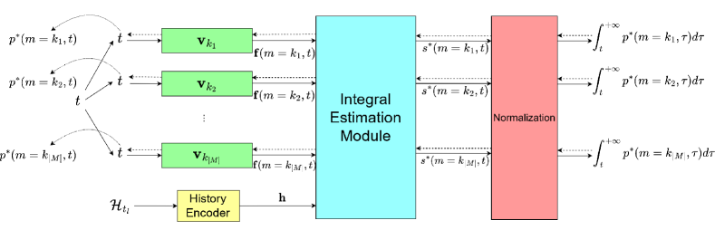
Figure 1: Architecture of IFIB-C. The solid arrows refer to forward propagation, the dashed arrows refer to backpropagation, and the curved dotted arrows refer to retrieving the gradient. The history encoder is an LSTM.

For each mark $m$, we assign a vector $\mathbf{v}_{m}$ to prepare $\mathbf{f}(m,t)=\mathbf{v}_{m}(t-t_{l})$ as input of the integral estimation module (IEM). IEM contains multiple fully-connected layers with non-negative weights and monotonic-increasing activation functions. It ends with a monotonically-decreasing sigmoid function $\sigma^{\prime}(x)=1/(1+e^{x})$ for each mark.

The outputs of IEM are scores $s^{*}(m=k_{1},t),s^{*}(m=k_{2},t),\cdots,s^{*}(m=k_{|\mathrm{M}|},t)$. The value of $\sum_{m\in\mathrm{M}}s^{*}(m,t)$ is not guaranteed to be 1. In order to produce the qualified probability distribution, they need to be normalized. This is achieved by Normalization module in Figure 1 that divides $s^{*}(m,t)$ by the partition function $Z(\mathcal{H}_{t_{l}})=\sum_{m\in\mathrm{M}}{s^{*}(m,t_{l})}$ for each $m\in M$. Finally, IFIB outputs $\Gamma^{*}(m,t)$ for each mark $m$ at the given time $t$:

$$\Gamma^{*}(m,t) =\int_{t}^{+\infty}{p^{*}(m,\tau)d\tau}=\frac{s^{*}(m,t)}{Z(\mathcal{H}_{t_{l}})}$$ (6)

$$p^{*}(m,t) =-\frac{1}{Z(\mathcal{H}_{t_{l}})}\frac{\partial\Gamma^{*}(m,t)}{\partial s^{*}(m,t)}\frac{\partial s^{*}(m,t)}{\partial\mathbf{f}(m,t)}\frac{\partial\mathbf{f}(m,t)}{\partial t}$$ (7)

Note that $p^{*}(m)$ in Equation 5 and $\Gamma^{*}(m,t)$ are distinct integrals. The former starts from $t_{l}$, the time of the last event in history, while the latter starts from time $t$, any time after $t_{l}$. When $t=t_{l}$, $p^{*}(m)$ is equivalent to $\Gamma^{*}(m,t)$ and $\sum_{m\in\mathrm{M}}p^{*}(m)=\sum_{m\in\mathrm{M}}\Gamma^{*}(m,t)=1$. The loss function of IFIB is Equation 8 that is the sum of the negative log-likelihood of $p^{*}(m,t)$ at every event $(m_{i},t_{i})\in\mathcal{S}$.

$$L=-\sum_{(m_{i},t_{i})\in\mathcal{S}}\log p^{*}(m_{i},t_{i}).$$ (8)

where $p^{*}(m_{i},t_{i})$ is the predicted probability after $(i-1)$th event.

4.2 IFIB-N

This section introduces IFIB-N, an IFIB variant for marked TPP where each mark is a vector in an $n$-dimensional continuous space, denoted as $\mathbf{m}=(d_{1},d_{2},\cdots,d_{n})$. IFIB-N outputs $\Gamma^{*}(\mathbf{m},t)$, the integral of $p^{*}(\mathbf{m},t)$ over time from $t$ and over n-dimensional continuous space from $\mathbf{m}$:

$$\Gamma^{*}(\mathbf{m},t) =\int_{\tau=t}^{+\infty}{\int_{r_{1}=d_{1}}^{b_{1}}\int_{r_{2}=d_{2}}^{b_{2}}\cdots\int_{r_{n}=d_{n}}^{b_{n}}{p^{*}(r_{1},r_{2},\cdots,r_{n},\tau)d\tau}dr_{1}dr_{2}\cdots dr_{n}}$$ (9)

where $p^{*}(\mathbf{m},t)$ is defined as follows:

$$p^{*}(\mathbf{m},t)=(-1)^{n+1}\frac{\partial}{\partial t}(\frac{\partial}{\partial d_{1}}(\frac{\partial}{\partial d_{2}}(\cdots(\frac{\partial\Gamma^{*}(\mathbf{m},t)}{\partial d_{n}}))))\\$$ (10)

However, we cannot devise an end-to-end model for estimating $\Gamma^{*}(\mathbf{m},t)$ as Equation 10 because such model’s ($n+1$)-rank derivative must be non-negative. This restriction eliminates most candidate functions while the remaining ones that could fulfill the restriction, like the exponential functions, are prone to enlarge the output and finally lead to the output explosion. Therefore, we propose a trick to split $\Gamma^{*}(\mathbf{m},t)$ into the product of integrals of $n+1$ conditional probability distributions, shown in Equation 11, each of which can be estimated separately. This trick dispenses the $n+1$ differentiation operations into the $n+1$ inputs, i.e., one differentiation operation for each input. Thus, we only need to affirm that the selected model could always estimate a normalized probability distribution.

$$\Gamma^{*}(\mathbf{m},t) =\int_{\tau=t}^{+\infty}{p^{*}(\tau)}d\tau{\int_{d_{1}}^{b_{1}}{p^{*}(r_{1}|\tau)}dr_{1}{\cdots\int_{d_{n}}^{b_{n}}{p^{*}(r_{n}|\tau,r_{1},r_{2},\cdots,r_{n-1})}}}dr_{n}$$ (11)

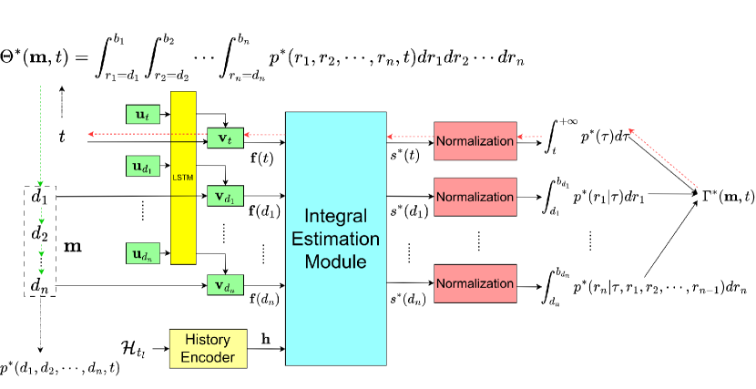
Figure 2: Architecture of IFIB-N. The solid, dashed, and dotted arrows are the same as in Figure 1. The history encoder is an LSTM.

Figure 2 depicts the structure of IFIB-N. For time $t$ and each dimension $i$ of mark $\mathbf{m}$, we allocate exclusive embedding vector $\mathbf{u}_{t}$ and $\mathbf{u}_{d_{i}}$. An LSTM module and a non-negative activation function are applied to produce non-negative $\mathbf{v}_{t}$ and $\mathbf{v}_{d_{i}}$ from $\mathbf{u}_{t}$ and $\mathbf{u}_{d_{i}}$ to disseminate conditional information to each probability distribution in Equation 11. The dot product of $t$ with $\mathbf{v}_{t}$ is $\mathbf{f}(t)$ which represents $p^{*}(\tau)$. The dot product of $d_{i}$ with $\mathbf{v}_{d_{i}}$ is $\mathbf{f}(d_{i})$ where $\mathbf{f}(d_{1})$, $\cdots$, $\mathbf{f}(d_{n})$ represent $p^{*}(r_{1}|\tau)$, $\cdots$, $p^{*}(r_{n}|\tau,r_{1},\cdots,r_{n-1})$, respectively. The IEM stays the same as in IFIB-C. For each of IEM outputs $s^{*}(t)$ and $s^{*}(d_{i})$, it has a Normalization module as in IFIB-C to ensure the output integral is normalized. Then, we multiply the integral of all conditional probabilities to form $\Gamma^{*}(\mathbf{m},t)$.

IFIB-N owns a unique backpropagation process to obtain $p^{*}(\mathbf{m},t)$. We elaborate this process in Algorithm 1. Briefly, it comprises two steps. First, we differentiate the final output by time $t$(represented by red dashed arrows in Figure 2) for $\Theta^{*}(\mathbf{m},t)$. Then, we obtain $p^{*}(\mathbf{m},t)$ by differentiating $\Theta^{*}(\mathbf{m},t)$ with every dimension of $\mathbf{m}$ (represented by grass green dashed arrows in Figure 2).

Algorithm 1 Obtain $p^{*}(\mathbf{m},t)$ from $\Gamma^{*}(\mathbf{m},t)$

  Input: Multi-dimensional Integral $\Gamma^{*}(\mathbf{m},t)$, input time $t$, input mark $\mathbf{m}=(d_{1},d_{2},\cdots,d_{n})$;

  $\Theta^{*}(\mathbf{m},t)=\partial\Gamma^{*}(\mathbf{m},t)/\partial t$;

  grad = $\Theta^{*}(\mathbf{m},t)$;

  for $d_{i}$ in $\mathbf{m}=(d_{1},d_{2},\cdots,d_{n})$ do

     grad = $\partial\text{grad}/\partial d_{i}$;

  end for

  $p^{*}(\mathbf{m},t)=\text{grad}$;

  return  $p^{*}(\mathbf{m},t)$

4.3 Why integral of distribution from $t$ to infinity?

Both IFIB-C and IFIB-N involve the integral of $p^{*}(\mathtt{m},t)$ from $t$ to positive infinity. One might raise questions about this design: what is the advantage of estimating the integral of $p^{*}(\mathtt{m},t)$ from $t$ to positive infinity? Why does not IFIB estimate the integral of $p^{*}(\mathtt{m},t)$ from $t_{l}$ to $t$?

Suppose we choose to estimate the integral of $p^{*}(\mathtt{m},t)$ from $t_{l}$ to $t$. Our model $\mathcal{M}$ must satisfy two restrictions: (1) output 0 when the input is $t_{l}$ as $\mathcal{M}(t_{l})=\int_{t_{l}}^{t_{l}}{p^{*}(\mathtt{m},\tau)d\tau}=0$, and (2) output no bigger than 1 as $t$ increases because $\lim_{t\rightarrow+\infty}{\mathcal{M}(t)}=\int_{t_{l}}^{+\infty}{p^{*}(\mathtt{m},\tau)d\tau}\in[0,1]$ Shchur et al. [2020]. While the latter is relatively easy, achieving the former is difficult since the output must be 0 when the input is $t_{l}$ regardless of the model parameter.

If we estimate the integral of $p^{*}(\mathtt{m},t)$ from $t$ to positive infinity, both restrictions are transformed into different restrictions. That is, our model $\mathcal{M}$ must (1) start from a positive number in $[0,1]$ because $\mathcal{M}(t_{l})=\int_{t_{l}}^{+\infty}{p^{*}(\mathtt{m},\tau)d\tau}\in[0,1]$, and (2) converge to 0 as $t$ goes larger because $\lim_{t\rightarrow+\infty}{\mathcal{M}(t)}=\lim_{t\rightarrow+\infty}\int_{t}^{+\infty}{p^{*}(\mathtt{m},\tau)d\tau}=0$. Such two restrictions are much easier for a model to comply with.

4.4 Applications

Given IFIB-C and IFIB-N, different applications regarding the mark and time of the next event can be performed. The widely studied application is to predict when the next event will occur and, once the time is determined, to predict which mark the next event is. We name it time-event prediction problem. Moreover, for each mark, if its probability of being the next event is non-zero, it is interesting to predict when the next event will occur conditioned on the fact that the next event is the mark. We name it event-time prediction problem. We explain how IFIB-C and IFIB-N solve these tasks in Appendix D.

5 Experiments on IFIB-C

In this section, we evaluate IFIB-C and baselines on four real-world datasets including Bookorder (BO) Du et al. [2016], Retweet Zhao et al. [2015], StackOverflow (SO) Leskovec and Krevl [2014], and MOOC Shchur et al. [2020]) and five synthetic datasets including Hawkes_1, Hawkes_2, Poisson, Self-correct, and Stationary Renewal Omi et al. [2019]. Detailed information about these datasets is available in Section F.1.

5.1 Evaluation Metrics

For real-world datasets, we utilize MAE (Mean Absolute Error) and macro-F1 for the time-event prediction problem and MAE-E (Mean Absolute Error by Event) and macro-F1 for the event-time prediction problem. To measure more reliably, we sort the prediction errors and report Q1, median, Q3 (i.e., $25$th, $50$th, $75$th percentile), denoted as MAE$@25\%$, MAE$@50\%$, MAE$@75\%$, respectively. We do the same for MAE-E. For the synthetic datasets, Spearman’s coefficient, $L^{1}$ distance, and the relative NLL loss are selected to gauge the difference between the learned $\hat{p}^{*}(m,t)$ and the real $p^{*}(m,t)$ as in Omi et al. [2019], Shchur et al. [2020]. Details of evaluation metrics are available in Section F.2.

5.2 Baseline Models

In this paper, we select six classic neural temporal point process models, Recurrent Marked Temporal Point Process(RMTPP) Du et al. [2016], Fully Neural Network(FullyNN)Omi et al. [2019], Fully Event Neural Network (FENN), Transformer Hawkes Process (THP)Zuo et al. [2020], LogNormMixShchur et al. [2020], and Self-Attentive Hawkes Process (SAHP)Zhang et al. [2020] as baselines. Detailed information about these approaches is available in Section F.3.

5.3 Experiment Results

We train IFIB-C and baselines on five synthetic datasets and gauge the gap between $\hat{p}(m,t)$ and $p(m,t)$ using Spearman coefficient and $L^{1}$ distance. The result shows that IFIB-C consistently learns more accurate distributions than all baselines. This conclusion gives us the confidence to apply IFIB-C to real-world datasets. Detailed experiment results are available in Section E.1.

Generally, the real-world data possess complicated temporal patterns and intricate correlations between marks which challenges the marked TPP modeling. This section trains IFIB-C and baselines on the four real-world datasets. They are evaluated by comparing the performances on two prediction problems discussed in Section 4.4, i.e., time-event (Table 3 and Table 4) and event-time (Table 1 Table 2). The numbers in bold or underlined indicate the best or the second-best value. We only report the time related performance of baseline RMTPP and LogNormMix in the time-event task because these models cannot determine the mark based on history $\mathcal{H}_{t_{l}}$ and time $t$. Meanwhile, as THP always returns meaningless outputs on Retweet, MOOC, and Bookorder, no result of THP on these datasets is reported.

5.3.1 Event-Time Prediction Problem

Table 1: Event-time prediction problem on real-world datasets measured by MAE-E$@x\%$($25\%,50\%,75\%$).

	IFIB(Ours)	FENN	FullyNN	SAHP	THP
Retweet	4.6142$\pm$0.0328	10.018$\pm$4.0837	16.092$\pm$7.5513	16.970$\pm$0.1569	/
	28.384$\pm$0.0825	50.755$\pm$15.025	70.959$\pm$28.580	116.05$\pm$5.4806	/
	232.96$\pm$1.0114	354.22$\pm$51.368	367.64$\pm$74.523	636.25$\pm$3.3811	/
SO	0.1179$\pm$0.0004	0.1672$\pm$0.0066	0.1530$\pm$0.0041	0.1377$\pm$0.0039	0.1535$\pm$0.0004
	0.2821$\pm$0.0009	0.4408$\pm$0.0121	0.3519$\pm$0.0052	0.3327$\pm$0.0075	0.3378$\pm$0.0004
	0.7597$\pm$0.0051	0.9103$\pm$0.0177	0.6717$\pm$0.0148	0.6795$\pm$0.0154	0.5531$\pm$0.1525
MOOC	4.2347$\pm$0.1265	1162.9$\pm$318.92	2704.8$\pm$190.60	3380.8$\pm$1782.2	/
	25.504$\pm$0.2938	4157.1$\pm$29.943	4277.2$\pm$6.8777	$>$ 500,000	/
	283.38$\pm$2.9122	4657.1$\pm$11.563	4653.4$\pm$14.971	$>$ 500,000	/
BO	0.0210$\pm$0.0007	200.53$\pm$0.1841	200.17$\pm$1.3407	0.0220$\pm$0.0019	/
	0.0298$\pm$0.0007	203.66$\pm$0.0000	203.66$\pm$0.0000	0.0469$\pm$0.0004	/
	0.2092$\pm$0.0008	203.71$\pm$0.0000	203.71$\pm$0.0000	0.2722$\pm$0.0184	/

In this test, we process each mark $m$ if its probability to be the next event is non-zero. On the condition that the mark of the next event is $m$, the time of the next event is predicted. For the real mark of the next event, the difference between the prediction and real-time is used to measure the performance, i.e., MAE-E. The results are in Table 1.

Table 2: Event-time prediction problem on real-world datasets measured by macro-F1.

	Retweet	SO	MOOC	BO
IFIB-C(Ours)	0.3576$\pm$0.0008	0.1085$\pm$0.0009	0.3684$\pm$0.0019	0.6021$\pm$0.0007
FullyNN	0.2316$\pm$0.0000	0.0121$\pm$0.0000	0.0005$\pm$0.0000	0.3339$\pm$0.0000
FENN	0.3646$\pm$0.0010	0.0930$\pm$0.0020	0.1698$\pm$0.0042	0.3902$\pm$0.0450
SAHP	0.3558$\pm$0.0021	0.1219$\pm$0.0050	0.2572$\pm$0.0312	0.5980$\pm$0.0009
THP	/	0.1373$\pm$0.0025	/	/

We can observe IFIB-C demonstrates superiority over baselines on all datasets. Compared with the results for the time-event prediction problem, the relative advantage of IFIB-C is more significant for the event-time prediction problem. As discussed in Section 4.4, the time prediction for a given mark is derived from Equation 30, which depends on the joint PDF $p^{*}(m,t)$. The well-suited $p^{*}(m,t)$ leads to a better time prediction. The results in Table 1 implicate that IFIB-C can model $p^{*}(m,t)$ in a better way than baselines. Further analysis of results in Table 1 are available in Appendix G.

In addition, the mark of the next event is predicted following Equation 31. The performances of IFIB-C and baselines measured in macro-F1 are reported in Table 2. IFIB-C retains its advantage over other integral-based methods. In summary, the event-time prediction performance further affirms that $\Gamma^{*}(m,t)$ in IFIB-C is a better estimation target than $\Lambda^{*}(t)$ in FENN.

5.3.2 Time-event Prediction Problem

Table 3: Time-event prediction performance on real-world datasets measured by MAE$@x\%$($25\%$, $50\%$, $75\%$).

	IFIB-C(Ours)	FENN	FullyNN	RMTPP	LogNormMix	SAHP	THP
Retweet	4.6309$\pm$0.0422	4.6344$\pm$0.0350	4.6957$\pm$0.0311	4.8436$\pm$0.0161	5.7855$\pm$0.7749	4.6991$\pm$0.0934	/
	28.545$\pm$0.0839	29.136$\pm$0.0352	28.575$\pm$0.1942	30.600$\pm$0.0134	28.380$\pm$1.0108	28.037$\pm$0.4119	/
	238.91$\pm$0.5870	255.62$\pm$2.5578	238.75$\pm$0.8049	269.90$\pm$0.9863	249.68$\pm$2.7573	261.44$\pm$7.6941	/
SO	0.1411$\pm$0.0010	0.1972$\pm$0.0009	0.1443$\pm$0.0011	0.1477$\pm$0.0026	0.1588$\pm$0.0128	0.1463$\pm$0.0014	0.1546$\pm$0.0004
	0.3347$\pm$0.0004	0.4287$\pm$0.0007	0.3352$\pm$0.0011	0.3397$\pm$0.0060	0.3624$\pm$0.0375	0.3422$\pm$0.0017	0.3394$\pm$0.0014
	0.6644$\pm$0.0043	0.6867$\pm$0.0017	0.6527$\pm$0.0013	0.6675$\pm$0.0069	0.7818$\pm$0.0464	0.6660$\pm$0.0007	0.6621$\pm$0.0005
MOOC	6.5689$\pm$0.0996	34.820$\pm$2.4208	5.8824$\pm$0.1621	19.217$\pm$0.9800	8.4106$\pm$0.9752	7.8945$\pm$1.1120	/
	38.795$\pm$1.4440	214.74$\pm$14.587	47.454$\pm$0.2333	147.15$\pm$5.6299	39.622$\pm$7.1465	135.49$\pm$17.609	/
	368.25$\pm$0.8369	825.98$\pm$24.410	386.98$\pm$4.8503	853.24$\pm$29.962	412.06$\pm$11.384	1262.1$\pm$273.55	/
BO	0.0213$\pm$0.0008	0.0138$\pm$0.0005	0.0138$\pm$0.0003	0.0603$\pm$0.0053	0.0167$\pm$0.0000	0.0190$\pm$0.0017	/
	0.0297$\pm$0.0007	0.0415$\pm$0.0006	0.0413$\pm$0.0003	0.1425$\pm$0.0020	0.0333$\pm$0.0000	0.0444$\pm$0.0010	/
	0.2091$\pm$0.0004	0.2391$\pm$0.0186	0.2488$\pm$0.0118	0.5189$\pm$0.0128	0.2112$\pm$0.0079	0.2353$\pm$0.0256	/

Table 4: Time-event prediction performance on real-world datasets measured by macro-F1.

	Retweet	SO	MOOC	BO
IFIB-C(Ours)	0.3530$\pm$0.0016	0.0797$\pm$0.0020	0.3499$\pm$0.0064	0.6002$\pm$0.0016
FENN	0.3468$\pm$0.0010	0.0147$\pm$0.0020	0.0951$\pm$0.0054	0.4006$\pm$0.0530
FullyNN	0.2315$\pm$0.0000	0.0121$\pm$0.0000	0.0005$\pm$0.0000	0.3339$\pm$0.0000
SAHP	0.3544$\pm$0.0020	0.1185$\pm$0.0040	0.3340$\pm$0.0109	0.6011$\pm$0.0006
THP	/	0.1380$\pm$0.0023	/	/

As in Equation 28 and Equation 29, the time-event prediction problem first predicts when the next event will happen, then predicts which mark the next event is most likely to be at the time. The metric for evaluating time prediction is MAE, and the metric for evaluating mark prediction is macro-F1. The test results are in Table 3 and Table 4.

As shown in Table 3, IFIB-C outperforms the integral-based methods (FENN and FullyNN) in general. It means IFIB-C provides more accurate time prediction for more events. Even in situations where IFIB-C does not show the best performance, the performance of IFIB-C is highly comparable. When compared with other baselines, IFIB-C demonstrates more significant advantages. This may be caused by the fact that these baselines are more or less affected by the intensity functions predefined.

In Table 4, IFIB-C beats all baselines in general in terms of macro-F1. It indicates IFIB-C is competent to time-event tasks. Looking closely, IFIB-C consistently defeats FENN. Considering the main difference between IFIB-C and FENN is that IFIB-C outputs $\Gamma^{*}(m,t)$ and FENN outputs $\Lambda^{*}(m,t)$, the test results provide evidence that $\Gamma^{*}(m,t)$ can be better estimated than $\Lambda^{*}(m,t)$.

6 Experiments on IFIB-N

We evaluated IFIB-N on five synthetic datasets, including Hawkes_1, Hawkes_2, Poisson, Self-correct, and Stationary Renewal Omi et al. [2019], and three real-world datasets including Earthquake, Citibike, and COVID-19 Chen et al. [2020]. Detailed information about these datasets is available in Section F.1. Our investigation did not identify proper baselines as most existing studies related to joint distribution $p^{*}(m,t)$ focus on categorical marks.

Since the mark is continuous, we cannot use macro-F1 to measure the mark prediction performance. Instead, we use DV (Distance between the predicted Vector and the ground truth) in pair with MAE and MAE-E mentioned in Section 5.1. We report Q1, Q2, and Q3 of DV, MAE, and MAE-E for reliable measurement. For the synthetic datasets, we use the same metrics, i.e., Spearman coefficient, $L^{1}$ distance, and relative NLL loss, to demonstrate that IFIB-N learns the true distribution $p^{*}(m,t)$ with high fidelity. Detailed information about all mentioned metrics is available in Section F.2, and we present all experiment results on synthetic datasets in Section E.2.

In Table 5 and Table 6, the performance of IFIB-N on three real-world datasets, Citibike, COVID-19, and Earthquake is reported. IFIB-N is the first marked TPP model that explicitly enforces normalized $p^{*}(\mathbf{m},t)$ and $P^{*}(\mathcal{C}(\mathbf{m}),t)$ for marks in a multi-dimensional continuous space. The results prove that IFIB-N could properly model $P^{*}(t)=\int_{t_{l}}^{t}{\int_{m\in\mathbf{M}}{p^{*}(\mathbf{m},\tau)d\mathbf{m}d\tau}}$ and $p^{*}(\mathbf{m},t)$ for the time-event prediction task, and properly model $p^{*}(m)=\int_{t_{l}}^{+\infty}{p^{*}(\mathbf{m},\tau)d\tau}$ and $P^{*}(\mathcal{C}(\mathbf{m}),t)$ for the event-time prediction task.

Table 5: Time-event prediction performance of IFIB-N on real-world datasets

		Citibike	COVID-19	Earthquake
MAE	MAE$@25\%$	0.0293$\pm$0.0000	0.0102$\pm$0.0001	0.0650$\pm$0.0015
	MAE$@50\%$	0.0607$\pm$0.0000	0.0216$\pm$0.0000	0.1646$\pm$0.0007
	MAE$@75\%$	0.1299$\pm$0.0001	0.0560$\pm$0.0004	0.3108$\pm$0.0007
DV	DV$@25\%$	0.5176$\pm$0.0003	3.5627$\pm$0.0361	3.0615$\pm$0.0684
	DV$@50\%$	0.5357$\pm$0.0002	3.7334$\pm$0.0205	6.3055$\pm$0.1422
	DV$@75\%$	0.5515$\pm$0.0004	3.9146$\pm$0.0276	10.379$\pm$0.2032

Table 6: Event-time prediction performance of IFIB-N on real-world datasets

		Citibike	COVID-19	Earthquake
MAE-E	MAE$@25\%$	0.0293$\pm$0.0000	0.0102$\pm$0.0001	0.0650$\pm$0.0015
	MAE$@50\%$	0.0607$\pm$0.0000	0.0216$\pm$0.0000	0.1646$\pm$0.0007
	MAE$@75\%$	0.1299$\pm$0.0001	0.0560$\pm$0.0004	0.3108$\pm$0.0007
DV	DV$@25\%$	0.5176$\pm$0.0003	3.5627$\pm$0.0361	3.0615$\pm$0.0684
	DV$@50\%$	0.5357$\pm$0.0002	3.7334$\pm$0.0205	6.3055$\pm$0.1422
	DV$@75\%$	0.5515$\pm$0.0004	3.9146$\pm$0.0276	10.379$\pm$0.2032

7 Conclusion

This paper proposed a framework IFIB to model joint conditional PDF $p^{*}(\mathtt{m},t)$ by exploring the relationship between $p^{*}(\mathtt{m},t)$ and its marginal probability of mark, i.e., $p^{*}(\mathtt{m})$, with neural networks. The advantages of IFIB have been demonstrated in three aspects. First, since no intensity function is involved, it remarkably simplifies the process to compel the essential mathematical restrictions. Second, it can be naturally applied to model TPP with categorical marks as well as numeric marks in a multi-dimensional continuous space. Third, it supports different applications regarding the time and mark prediction of the next event. In the future study, we plan to extend IFIB to model marked TPP problems that encounter the complex mark with both categorical information and numeric values in a multi-dimensional continuous space, for example, the observations of different species in a spatial region over time.

Appendix A The Conditional Joint PDF

Without loss of generality, we assume the mark is categorical. For mark $m$, we define a conditional intensity function $\lambda^{*}(m,t)$:

$$\lambda^{*}(m=k_{i},t)=\lambda(m=k_{i},t|\mathcal{H}_{t})$$ (12)

$$=\lim_{\Delta t\rightarrow 0}{\frac{P(m=k_{i},t\in[t,t+\Delta t)|\mathcal{H}_{t-})}{\Delta t}}$$

$$=\lim_{\Delta t\rightarrow 0}{\frac{p(m=k_{i},t\in[t,t+\Delta t)|\mathcal{H}_{t_{l}})\Delta t}{P(\forall j\in\mathbb{N}^{+},t_{j}\notin(t_{l},t)|\mathcal{H}_{t_{l}})\Delta t}}$$

$$=\lim_{\Delta t\rightarrow 0}{\frac{p(m=k_{i},t\in[t,t+\Delta t)|\mathcal{H}_{t_{l}})}{P(\forall j\in\mathbb{N}^{+},t_{j}\notin(t_{l},t)|\mathcal{H}_{t_{l}})}}$$

$$=\frac{p(m=k_{i},t\in[t,t+dt)|\mathcal{H}_{t_{l}})}{P(\forall j\in\mathbb{N}^{+},t_{j}\notin(t_{l},t)|\mathcal{H}_{t_{l}})}$$

where $\mathcal{H}_{t_{l}}$ is the history up to (including) the most recent event, $\mathcal{H}_{t-}$ is the history up to (excluding) the current time, $P(\forall j\in\mathbb{N}^{+},t_{j}\notin(t_{l},t)|\mathcal{H}_{t_{l}})$ represents the probability that no event is observed in time interval $(t_{l},t)$ given $\mathcal{H}_{t_{l}}$.

We denote $P^{{}^{\prime}}_{m}((t_{1},t_{2})|\mathcal{H}_{t_{l}})$ for the conditional probability that an event $m$ happens in $(t_{1},t_{2})$. Following the definition of simple TPP that at most one event happens at every timestamp $t$, the probability that no event occurs in $(t_{l},t)$ is:

$$P(\forall j\in\mathbb{N}^{+},t_{j}\notin(t_{l},t)|\mathcal{H}_{t_{l}})$$ (13)

$$=1-\sum_{w\in\mathrm{M}}{P^{{}^{\prime}}_{w}((t_{l},t)|\mathcal{H}_{t_{l}})\prod_{n\in\mathrm{M},n\neq w}({1-P^{{}^{\prime}}_{n}((t_{l},t)|\mathcal{H}_{t_{l}})})}$$

$$=1-\sum_{w\in\mathrm{M}}{\frac{P^{{}^{\prime}}_{w}((t_{l},t)|\mathcal{H}_{t_{l}})}{1-P^{{}^{\prime}}_{w}((t_{l},t)|\mathcal{H}_{t_{l}})}}\prod_{n\in M}({1-P^{{}^{\prime}}_{n}((t_{l},t)|\mathcal{H}_{t_{l}})})$$

$$=1-\sum_{w\in\mathrm{M}}{P(w,t|\mathcal{H}_{t_{l}})}=1-\sum_{w\in\mathrm{M}}{P^{*}(w,t)}$$

where

$$P^{*}(w,t)=\frac{P^{{}^{\prime}}_{w}((t_{l},t)|\mathcal{H}_{t_{l}})}{1-P^{{}^{\prime}}_{w}((t_{l},t)|\mathcal{H}_{t_{l}})}\prod_{n\in\mathrm{M}}({1-P^{{}^{\prime}}_{n}((t_{l},t)|\mathcal{H}_{t_{l}}))}$$ (14)

The conditional joint PDF that the next event is $m$ and occurs in $[t,t+dt)$ is:

$$p(m=k_{i},t\in[t,t+\Delta t)|\mathcal{H}_{t_{l}})=\frac{dP^{*}(m=k_{i},t)}{dt}$$ (15a)

$$\int_{t_{l}}^{t}{p(m=k_{i},t\in[t,t+\Delta t)|\mathcal{H}_{t_{l}})d\tau}=P^{*}(m=k_{i},t)$$ (15b)

In this study, $p^{*}(m,t)$, shorthand of $p(m,t|\mathcal{H}_{t_{l}})$, is the formal representation of $p(m=k_{i},t\in[t,t+\Delta t)|\mathcal{H}_{t_{l}})$. Note $P^{*}(m,t)$ in Equation 14 is the probability that only one event happens in interval $[t,t+dt)$ and the mark is $m$. This ensures the marked TPP represented by $p^{*}(m,t)$ is simple. By integrating Equation 15a and LABEL:eqn:noevent in LABEL:eqn:lambda_i, we have

$$p^{*}(m,t)=\lambda^{*}(m,t)(1-\sum_{w\in\mathrm{M}}{P^{*}(w,t)})$$ (16)

where $\sum_{w\in\mathrm{M}}{P^{*}(w,t)})$ is calculated from the sum of LABEL:eqn:lambda_i over marker $m$:

$$\sum_{w\in\mathrm{M}}{P^{*}(w,t)}=1-\exp(-\int_{t_{l}}^{t}{\sum_{n\in\mathrm{M}}{\lambda^{*}(n,\tau)}d\tau})$$ (17)

Then, we solve $p^{*}(m,t)$:

$$p^{*}(m,t)=\lambda^{*}(m,t)\exp(-\int_{t_{l}}^{t}{\sum_{n\in\mathrm{M}}{\lambda^{*}(n,\tau)}d\tau})$$ (18)

which is equivalent with Equation 2. We won’t go into details about numeric marks but directly provide the expression of joint PDF $p(\mathbf{m},t)$ in Equation 19. One could replace the summation of all categorical marks by the integration over the multi-dimensional continuous space to smoothly adapt the conclusion for categorical marks to the numeric marks.

$$p^{*}(\mathbf{m},t)=\lambda^{*}(\mathbf{m},t)\exp(-\int_{t_{l}}^{t}{\int_{\mathbf{n}\in\mathbf{M}}{\lambda^{*}(\mathbf{n},\tau)}d\tau d\mathbf{n}})$$ (19)

Appendix B Analysis on FullyNN and FENN

The analysis is based on categorical marks only since FullyNN and FENN cannot handle numeric marks in multi-dimensional continuous space.

B.1 Why FullyNN incapable of marked TPP

FullyNN sets the learning target of NNs to $\Lambda^{*}(t)$, the integral of intensity functions $\lambda^{*}(t)$. This idea works when no event mark information is present. However, when we require FullyNN to learn different intensity functions for different event marks, the limitation emerges as FullyNN cannot allocate different computation graphs for different marks.

To understand this, we should recognize how FullyNN calculates the intensity function. Following the definition in Omi et al. [2019], a FullyNN can be written in the following expression:

$$\Lambda^{*}(t)=\operatorname{FullyNN}(t,\mathbf{h})=\operatorname{IEM}(\mathbf{f}(t),\mathbf{h})$$ (20)

where $\mathbf{f}(t)$ represents a monotonic-increasing function mapping the time $t$ into a vector, $\mathbf{h}$ is the history embedding, and $\operatorname{IEM}$ refers to the integral estimation module. From Equation 20, we could derive the intensity function as:

$$\lambda^{*}(t)=\frac{\partial\Lambda^{*}(t)}{\partial t}=\frac{\partial\operatorname{IEM}(\mathbf{f}(t),\mathbf{h})}{\partial\mathbf{f}(t)}\frac{\partial\mathbf{f}(t)}{\partial t}$$ (21)

If one generalizes the FullyNN from mark-agnostic to mark-aware by simply expanding the input time from $t$ to $\mathbf{t}=[t,t,t,\cdots,t]^{\top}$, each for one of the $|\mathrm{M}|$ marks, and they share the same vector $\mathbf{v}$ for generating the same $\mathbf{f}(t)$s as input of IEM. By letting the corresponding intensity integral be $\mathbf{\Lambda}^{*}(\mathbf{t})=[\Lambda^{*}(m=k_{1},t),\Lambda^{*}(m=k_{2},t),\Lambda^{*}(m=k_{3},t),\cdots,\Lambda^{*}(m=k_{|\mathrm{M}|},t)]^{\top}$, we could find the Jacobian Matrix $D_{\mathbf{t}}\mathbf{\Lambda}^{*}(t)$ is:

$$D_{\mathbf{t}}\mathbf{\Lambda}^{*}(\mathbf{t})$$ (22)

$$=\frac{\partial[\Lambda^{*}(m=k_{1},t),\Lambda^{*}(m=k_{2},t),\cdots,\Lambda^{*}(m=k_{|M|},t)]^{\top}}{\partial\mathbf{t}}$$

$$=\begin{pmatrix}\frac{\partial\operatorname{IEM(\mathbf{f}(t),\mathbf{h})}}{\partial\mathbf{f}(t)}\mathbf{v}&0&\cdots&0\\ 0&\frac{\partial\operatorname{IEM(\mathbf{f}(t),\mathbf{h})}}{\partial\mathbf{f}(t)}\mathbf{v}&\cdots&0\\ \vdots&\vdots&\ddots&\vdots\\ 0&0&\cdots&\frac{\partial\operatorname{IEM(\mathbf{f}(t),\mathbf{h})}}{\partial\mathbf{f}(t)}\mathbf{v}\\ \end{pmatrix}$$

which implies that the intensity functions for different marks receive identical distributions, and the event prediction performance would be stuck at $\frac{1}{|\mathrm{M}|}$. We believe this might explain the shockingly bad event prediction performance in Enguehard et al.’s paper Enguehard et al. [2020].

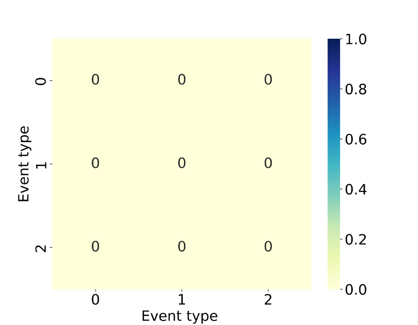
(a) FullyNN on Retweet dataset.

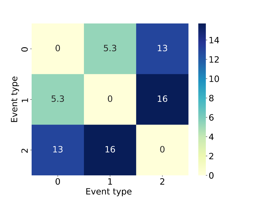
(b) FENN on Retweet dataset.

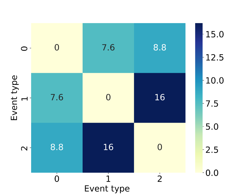
(c) IFIB-C on Retweet dataset.

Figure 3: The $L^{1}$ distance between distribution $p^{*}(m_{i},t)$ and distribution $p^{*}(m_{j},t)$, for each pair of marks ($m_{i},m_{j}$) in $\mathrm{M}$, generated by FullyNN, FENN and IFIB-C on an event sequence in Retweet dataset. FullyNN generates the identical distribution for different marks as the $L^{1}$ distance between $p^{*}(m_{i},t)$ and $p^{*}(m_{j},t)$ is 0 for each pair of marks ($m_{i},m_{j}$) in $\mathrm{M}$. In contrast, FENN and IFIB-C generate different distributions for different marks.

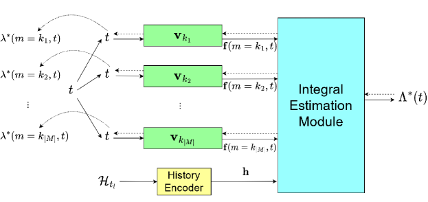
Figure 4: Architecture of Fully Event Neural Network (FENN). The solid arrows refer to forward propagation, the dashed arrows refer to backpropagation, and the curved arrows refer to retrieving the gradient. FENN models $\Lambda^{*}(t)$ and obtains $\lambda^{*}(m,t)$ by backpropagation.

B.2 Fully Event Neural Network

To handle marks in a better way, FullyNN can be extended to FENN (Fully Event Neural Network), which models $p^{*}(m,t)$ based on the conditional intensity $\lambda^{*}(m,t)$ as defined in Equation 2. FENN is sketched in Figure 4. The history $\mathcal{H}_{t_{l}}$ is represented as an embedding $\mathbf{h}$ using a LSTM encoder Omi et al. [2019]. FENN needs to model $|\mathrm{M}|$ conditional intensity functions, i.e., $\lambda^{*}(m,t)$ for all $m\in\mathrm{M}$. The integral of conditional intensity functions across all marks, from the time of the latest event $t_{l}$ to the current time $t$, is denoted as $\Lambda^{*}(t)$. The definition of $\Lambda^{*}(t)$ is given in LABEL:eqn:fete_integral, and the relationship between $\Lambda^{*}(t)$ and $\lambda^{*}(m,t)$ is presented in Equation 23b:

$$\begin{split}&\Lambda^{*}(t)=\int_{t_{l}}^{t}{\sum_{n\in\mathrm{M}}{\lambda^{*}(n,\tau)}d\tau}=\\ &\operatorname{IEM_{FENN}}(\mathbf{f}(m=k_{1},t),t),\cdots,\mathbf{f}(m=k_{|\mathrm{M}|},t),\mathbf{h}),\end{split}$$ (23a)

$$\lambda^{*}(m,t)=\frac{\partial\Lambda^{*}(t)}{\partial\mathbf{f}(m,t)}\frac{\partial\mathbf{f}(m,t)}{\partial t},\ \text{for}\ m\in\mathrm{M}.$$ (23b)

where $\mathbf{f}(m,t)$ is defined as $\mathbf{v}_{m}(t-t_{l})$ for mark $m\in\mathrm{M}$. FENN utilizes $\mathbf{v}_{m}$ to distinguish event marks to avoid sharing the same computation graph as FullyNN. The integral estimation module (IEM) of FENN contains multiple fully-connected layers with non-negative weights and monotonic-increasing activation functions and ends with an unbounded above softplus function $\operatorname{softplus}(x)=\log(1+e^{x})$. IEM receives history embedding $\mathbf{h}$ and $\mathbf{f}(m=k_{1},t),\mathbf{f}(m=k_{2},t),\cdots,\mathbf{f}(m=k_{|\mathrm{M}|},t)$, outputs $\Lambda^{*}(t)$. The loss function of FENN is the negative logarithm of $p^{*}(m,t)$ at every known event $(m_{i},t_{i})\in\mathcal{S}$, as shown in Equation 24.

$$L =\sum_{(m_{i},t_{i})\in\mathcal{S}}{-\log p^{*}(m_{i},t_{i})}$$ (24)

$$=\sum_{(m_{i},t_{i})\in\mathcal{S}}{(-\log\lambda^{*}(m_{i},t_{i})+\int_{t_{l}}^{t_{i}}{\lambda^{*}(m,\tau)d\tau})}$$

FENN inherits from FullyNN the capability to instantaneously provide accurate $\lambda^{*}(m,t)$ and the integral $\Lambda^{*}(t)$, and FENN solves the computation graph overlap issue in FullyNN as evidenced by the test results in Figure 3. However, FENN also inherits the weakness of FullyNN: it violates several essential mathematical restrictions Shchur et al. [2020]. To elaborate on this, we first rewrite LABEL:eqn:fete_integral by expanding $\operatorname{IEM_{FENN}}(\cdot)$.

$$\Lambda^{*}(t) =\sum_{m\in M}{\operatorname{softplus}(\Omega^{*}(m,t)+b)}$$ (25a)

$$\Omega^{*}(m,t) =\mathbf{w}^{\top}\operatorname{tanh}(\mathcal{F}_{l}(\cdots\mathcal{F}_{2}(\mathcal{F}_{1}([\mathbf{v}_{m}(t-t_{l}),\mathbf{h}])))).$$ (25b)

$$\mathcal{F}_{i}(\mathbf{x}) =\operatorname{tanh}(\mathbf{W}_{i}\mathbf{x}+\mathbf{b}_{i})$$ (25c)

where $\mathbf{W}_{i}$ and $\mathbf{w}$ are matrices and vectors, respectively, without negative numbers, $\mathbf{b}_{i}$ and $b$ are biases, and $l$ is the number of non-negative fully-connected layers. With the two expressions above, we reveal the restrictions that FENN fails to compel:

1. The IEM must output 0 when the input is exactly $t_{l}$. Otherwise, the model allows future events to occur before the latest historical event, which is unreasonable. Unfortunately, as $\operatorname{softplus}(x)=\log(1+e^{x})$ is always positive, $\Lambda^{*}(t_{l})$ would be close to, but never be 0.

2. The model’s output must be unbounded, in other words, $\lim_{t\rightarrow+\infty}\Lambda^{*}(t)=+\infty$ because the cumulative distribution function, $P^{*}(t)=\int_{t_{l}}^{t}{\sum_{n\in M}p^{*}(n,\tau)d\tau}=1-\exp(-\Lambda^{*}(t))$, must converge to 1 as $t\rightarrow+\infty$ if assuming the next event always happens. However, similar to FullyNN, because FENN’s activation function between the fully-connected layers is $\tanh(x)$, whose value domain is $(-1,1)$, the upper bound of $\Lambda^{*}(t)$ exists as shown in Equation 26, resulting in an unnormalized probability distribution.

   $$\Lambda^{*}(t)_{max}=\sum_{m\in M}{\operatorname{softplus}(\mathbf{w}_{1}^{\top}\mathbf{1}+b_{1})}<+\infty$$ (26)

Moreover, these restrictions are parameter-independent, meaning that one must directly impose them into the model structure, making them more difficult to deal with. In conclusion, although FENN can provide the conditional joint PDF $p^{*}(m,t)$, its structure is still faulty, which could lead to inferior performance.

Appendix C Analysis on LogNormMix

The intensity-free mindset focuses on directly modelling probability distribution while ignoring the intrinsic theory of TPP. LogNormMix Shchur et al. [2020], powered by this mindset, models the probability of $p^{*}(t)$ by a composition of log-normal distributions, whose means and variances derive from history. This approach performs well on synthetic and real-world TPP tasks with closed-form distributions that help it free from intensity estimation.

These fantastic features propel us to adapt the intensity-free mindset to our task in this paper. Given a categorical mark $m$, the original approach in Shchur et al. [2020] learns a distribution $p^{*}(m)$ independent from the time distribution $p^{*}(t)$ for event prediction. Such a design removes the connection between mark and time, which may harm the model’s performance.

Therefore, it is intuitive to ask whether we could slightly modify LogNormMix to fit the marked TPP by setting up $|\mathrm{M}|$ probability distributions for $|\mathrm{M}|$ categorical markers. Specifically, instead of splitting $p^{*}(m,t)$ into two independent distributions, we want to directly extract $p^{*}(m,t)$ from the training data like what IFIB-C does. Unfortunately, we cannot do that by following the current mindset of LogNormMix.

Why? Unlike TPP, the marked TPP concerns the conditional joint PDF $p^{*}(m,t)$ where the integral over time and marks should be 1, as shown in Equation 27.

$$\sum_{m\in\mathrm{M}}{\int_{t_{l}}^{+\infty}{p^{*}(m,\tau)}d\tau}dm=1$$ (27)

This equation indicates that $p^{*}(m)=\int_{t_{l}}^{+\infty}{p^{*}(m,t)}$ for mark $m$ should dwell in $(0,1)$, and $\sum_{m\in\mathrm{M}}p^{*}(m)$ is always 1. However, the mindset of LogNormMix assigns a complete probability distribution $q_{m}(t)$ to each mark $m$ where $q_{m}(t)$’s integral from $t_{l}$ to infinity is already 1. So $\sum_{m\in\mathrm{M}}{\int_{t_{l}}^{+\infty}{q_{m}(\tau)}d\tau}=|\mathrm{M}|$. This violates Equation 27. For the same reason, since $q_{m}(t)$ is a complete distribution and independent, whenever we optimise $q_{m}(t)$ by minimising its negative logarithm for event $(m_{i},t_{i})$, $q_{m_{i}}(t)$ receives the information to maximize $q_{m_{i}}(t_{i})$ but the information to update $q_{m_{j}}(t)$ is inevitably lost. In conclusion, it is unknown to us how to extend LogNormMix to model $p^{*}(m,t)$ problem without significant effort.

Appendix D Applications of IFIB

In this section, we discuss how IFIB-C and IFIB-N solve the time-event prediction problem and event-time prediction problem in Section 4.4.

D.1 Applications with IFIB-C

To answer the time-event prediction problem with IFIB-C, we first obtain $P^{*}(t)$, the probability of an event happening between $t_{l}$ and $t$, as follows:

$$P^{*}(t) =1-\sum_{m\in\mathrm{M}}{\int_{t}^{+\infty}{p^{*}(m,\tau)d\tau}}$$ (28)

For the time-event prediction problem, we follow the criterion in Omi et al. [2019] by selecting the minimum $t_{p}$ that allows $P^{*}(t_{p})\geqslant 0.5$. Because $P^{*}(t)$ is a monotonical function, we could efficiently obtain $t_{p}$ using the bisection method. Then, the mark of the next event at $t_{p}$ can be predicted.

$$m_{p} =\operatorname*{arg\,max}_{m}{p^{*}(m|t_{p})}=\operatorname*{arg\,max}_{m}{\frac{p^{*}(m,t_{p})}{\sum_{n\in\mathrm{M}}p^{*}(n,t_{p})}}$$ (29)

For the event-time prediction problem, we require the probability of an event marked by $m$ happening between $t_{l}$ and $t$ denoted as $P^{*}(t|m)$. It involves $P^{*}(m)$, the integral of $p^{*}(m,t)$ from $t_{l}$ to positive infinity, and $P^{*}(m,t)$, the integral of $p^{*}(m,t)$ from $t_{l}$ to $t$ given $m$. Equation 30 shows the expression of $P^{*}(t|m)$.

$$P^{*}(t|m)=\frac{P^{*}(m,t)}{P^{*}(m)}=\frac{1}{\int_{t_{l}}^{+\infty}{p^{*}(m,\tau)d\tau}}\int_{t_{l}}^{t}{p^{*}(m,\tau)d\tau}$$ (30)

$$\int_{t_{l}}^{t}{p^{*}(m,\tau)d\tau}=\int_{t_{l}}^{+\infty}{p^{*}(m,\tau)d\tau}-\int_{t}^{+\infty}{p^{*}(m,\tau)d\tau}$$

For each mark $m$, resembling how we obtain $t$ from Equation 29, the minimum $t_{p}$ such that $P^{*}(t_{p}|m)\geqslant 0.5$ is reported as the expected time that the next event will occur on the condition that the mark is $m$. Since $P^{*}(t|m)$ is monotonic, it is also solvable by the bisection method. Meanwhile, we can predict which mark is more likely to be the next event.

$$m_{p} =\operatorname*{arg\,max}_{m}{p^{*}(m)}=\operatorname*{arg\,max}_{m}{\int_{t_{l}}^{+\infty}{p^{*}(m,\tau)}d\tau}$$ (31)

Once $m_{p}$ is known, the time of the next event can be estimated using Equation 30.

D.2 Applications with IFIB-N

IFIB-N solves the time-event prediction problem in a similar way as IFIB-C. It starts from obtaining $P^{*}(t)$, the probability that an event with whatever mark could happen in the time interval $(t_{l},t)$, as follows:

$$P^{*}(t)=1-\int_{t}^{+\infty}{\int_{\mathbf{r}\in\mathbf{M}}{p^{*}(\mathbf{r},\tau)d\tau d\mathbf{r}}}$$ (32)

We then follow the criterion proposed by Omi et al. [2019], determining that an event happens once $P^{*}(t_{p})\geqslant 0.5$. $P^{*}(t)$ is monotonic, so we could employ the bisect method to solve $t_{p}$ efficiently. As for what mark this event would be, we probe the probability distribution $p^{*}(\mathbf{m},t_{p})$ in the $n$-dimensional continuous space and output the mark $\mathbf{m}$ so that $p^{*}(\mathbf{m},t)$ hits the maximum.

$$\mathbf{m}_{p}=\operatorname*{arg\,max}_{\mathbf{m}}{p^{*}(\mathbf{m},t_{p})}$$ (33)

Solving the event-time prediction problem with IFIB-N encounters an issue that the value of $p(\mathbf{m})=\int_{t_{l}}^{t}{p^{*}(\mathbf{m},\tau)d\tau}$ at every $\mathbf{m}$ is infinitesimal because there are infinite marks in the $n$-dimensional continuous space. Computers have difficulty handling infinitesimal. So, we replace $p(\mathbf{m})$ with the probability in a small hypercube $\mathcal{C}(\mathbf{m})$ in $\mathbf{M}$. This cube centers at $\mathbf{m}$ with a very small edge. Now we can write the expression of $P^{*}(t|\mathbf{m})$ as follows:

$$P^{*}(t|\mathbf{m})=\frac{P^{*}(\mathbf{m},t)}{P^{*}(\mathbf{m})}\\ =1-\frac{\int_{t}^{+\infty}\int_{\mathbf{r}\in\mathcal{C}(\mathbf{m})}{p^{*}(\mathbf{r},\tau)}d\tau d\mathbf{r}}{\int_{t_{l}}^{+\infty}\int_{\mathbf{r}\in\mathcal{C}(\mathbf{m})}{p^{*}(\mathbf{r},\tau)}d\tau d\mathbf{r}}\\$$ (34)

For each probed mark $\mathbf{m}$, we apply bisect method to find the minimum $t_{p}$ so that $P^{*}(t_{p}|\mathbf{m})\geqslant 0.5$. Meanwhile, we can effectively find the mark $\mathbf{m}_{p}$ of the next event by, resembling Equation 33, probing where $p^{*}(\mathbf{m},t_{l})$ hits its maximum.

$$\mathbf{m}_{p}=\operatorname*{arg\,max}_{\mathbf{m}}p^{*}(\mathbf{m},t_{l})=\operatorname*{arg\,max}_{\mathbf{m}}{\int_{t_{l}}^{+\infty}{p^{*}(\mathbf{m},\tau)d\tau}}$$ (35)

After replacing $\mathbf{m}$ in Equation 34 with $\mathbf{m}_{p}$ and solving $t_{p}$, we figure out the event-time prediction task by IFIB-N.

Table 7: Performance on synthetic datasets (higher Spearman, lower $L^{1}$, and lower relative NLL loss are better.)

		Hawkes_1	Hawkes_2	Poisson	Self-correct	Stationary Renewal
Spearman	IFIB-C(Ours)	1.0000$\pm$0.0000	0.9999$\pm$0.0000	1.0000$\pm$0.0000	0.9551$\pm$0.0009	0.9999$\pm$0.0000
	FENN	0.9946$\pm$0.0004	0.9964$\pm$0.0002	0.9736$\pm$0.0006	0.9473$\pm$0.0010	0.9998$\pm$0.0000
	FullyNN	0.9952$\pm$0.0004	0.9963$\pm$0.0002	0.9722$\pm$0.0018	0.9477$\pm$0.0001	0.9998$\pm$0.0000
	RMTPP	0.9839$\pm$0.0000	0.8473$\pm$0.0001	1.0000$\pm$0.0000	0.9557$\pm$0.0001	0.0204$\pm$0.0000
	LogNormMix	0.9816$\pm$0.0000	0.9772$\pm$0.0000	0.9685$\pm$0.0002	0.9462$\pm$0.0000	0.9999$\pm$0.0000
	SAHP	0.9959$\pm$0.0047	0.9862$\pm$0.0000	0.9615$\pm$0.0025	0.9492$\pm$0.0014	0.9990$\pm$0.0007
	THP	0.9266$\pm$0.0026	0.7366$\pm$0.0005	1.0000$\pm$0.0000	0.6969$\pm$0.0017	0.0413$\pm$0.0024
$L^{1}$	IFIB-C(Ours)	0.1480$\pm$0.0085	0.3105$\pm$0.0432	0.0133$\pm$0.0091	0.7907$\pm$0.0711	0.0654$\pm$0.0018
	FENN	0.6248$\pm$0.0052	3.0398$\pm$0.0693	0.2919$\pm$0.0051	1.2139$\pm$0.1652	0.0703$\pm$0.0058
	FullyNN	0.6235$\pm$0.0227	3.1048$\pm$0.0763	0.2973$\pm$0.0098	1.1889$\pm$0.0244	0.0710$\pm$0.0099
	RMTPP	5.1690$\pm$0.0028	21.144$\pm$0.0115	0.0469$\pm$0.0111	0.7193$\pm$0.0329	9.7272$\pm$0.0031
	LogNormMix	0.8767$\pm$0.0038	4.2257$\pm$0.0338	0.3861$\pm$0.0036	1.1145$\pm$0.0301	0.0405$\pm$0.0056
	SAHP	1.0245$\pm$0.2967	4.7867$\pm$0.2735	0.6893$\pm$0.0238	1.3363$\pm$0.0196	0.4872$\pm$0.1833
	THP	12.003$\pm$0.2069	25.500$\pm$0.3642	0.0203$\pm$0.0067	10.656$\pm$0.0965	9.9230$\pm$0.0451
Relative NLL	IFIB-C(Ours)	0.0000$\pm$0.0000	0.0001$\pm$0.0000	0.0000$\pm$0.0000	0.0007$\pm$0.0003	0.0000$\pm$0.0000
	FENN	0.0003$\pm$0.0000	0.0009$\pm$0.0001	0.0002$\pm$0.0000	0.0016$\pm$0.0006	0.0000$\pm$0.0000
	FullyNN	0.0003$\pm$0.0000	0.0008$\pm$0.0001	0.0002$\pm$0.0000	0.0015$\pm$0.0001	0.0000$\pm$0.0000
	RMTPP	0.0586$\pm$0.0000	0.3653$\pm$0.0000	0.0000$\pm$0.0000	0.0003$\pm$0.0000	0.0615$\pm$0.0000
	LogNormMix	0.0001$\pm$0.0000	0.0002$\pm$0.0000	0.0000$\pm$0.0000	0.0010$\pm$0.0000	0.0000$\pm$0.0000
	SAHP	0.0086$\pm$0.0017	0.0312$\pm$0.0193	0.0092$\pm$0.0002	0.0072$\pm$0.0009	0.0034$\pm$0.0010
	THP	0.2137$\pm$0.0001	0.6663$\pm$0.0029	0.0000$\pm$0.0000	0.1262$\pm$0.0004	0.0771$\pm$0.0000

Appendix E Experiment results on synthetic datasets

E.1 Results on IFIB-C

Synthetic datasets can help us verify whether a marked TPP model works correctly. To this end, we compare the real $p^{*}(m,t)$ of each synthetic dataset with $\hat{p}^{*}(m,t)$ modeled using IFIB-C and baselines. The selected metrics are Spearman’s coefficient, $L^{1}$ distance, and relative NLL loss. The results are reported in Table 7. The numbers in bold or underlined indicate the best or the second-best value.

IFIB-C, FullyNN, FENN, SAHP, and LogNormMix can consistently return correct $p^{*}(m,t)$ in most situations as their Spearman’s coefficient is close to 1, and their $L^{1}$ distance is also acceptable. On the other hand, RMTPP and THP struggle to learn the correct distribution on some synthetic datasets. The limitation of the presumed fixed-form intensity function may cause this.

The results demonstrate that IFIB-C always learns marked TPP models with high fidelity, which consistently have the best $L^{1}$ distance, negative NLL loss, and Spearman’s coefficient in almost all cases. Only RMTPP and Lognormmix defeat IFIB-C on the self-correct and stationary renewal dataset. FENN and FullyNN also perform strongly from the perspective of relative NLL loss, but the values in $L^{1}$ distance reveal that FENN and FullyNN cannot perfectly estimate $p^{*}(m,t)$ at every $t$. Specifically, $\hat{p}^{*}(m,t)$ around $t_{l}$ might deviate from $p^{*}(m,t)$. In contrast, IFIB-C successfully avoids this issue. This can be observed clearly when we compare $\hat{p}^{*}(m,t)$ and $p^{*}(m,t)$ at every time in a short time period after $t_{l}$, as shown in Figure 5 where $0$ in x-axis is $t_{l}$. More experiments (not reported) prove that such deviations exist in all synthetic datasets.

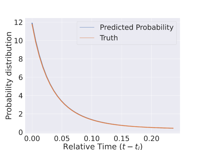
(a) IFIB

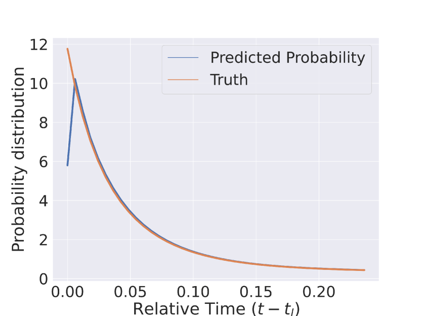
(b) FENN

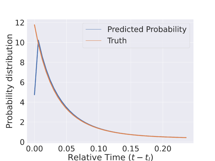
(c) FullyNN

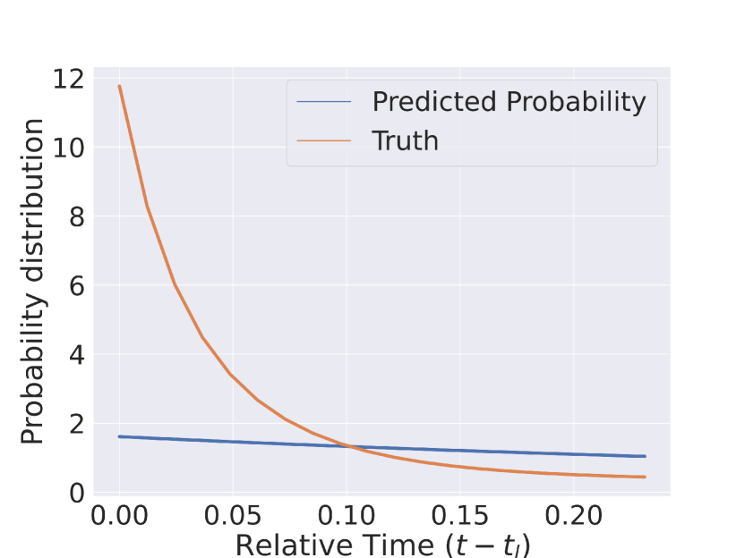
(d) RMTPP

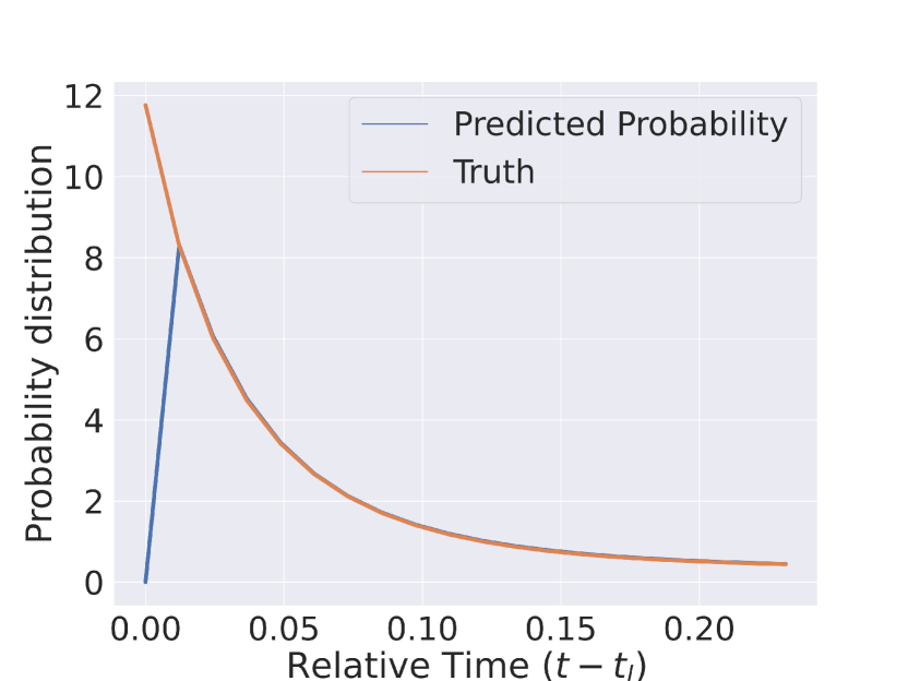
(e) LogNormMix

(f) SAHP

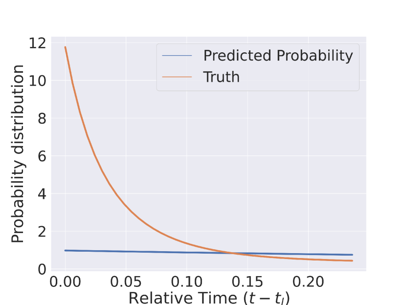
(g) THP

Figure 5: Curves of $\hat{p}^{*}(m,t)$ and $p^{*}(m,t)$ around $t_{l}$ on Hawkes_2. We notice that FullyNN, FENN, and LogNormMix often start from an unusually low value at $t_{l}$ before returning to the correct values, causing a high $L^{1}$ distance and low Spearman’s coefficient. The relative NLL loss, on the other hand, cannot reflect this phenomenon in its value.

E.2 Results on IFIB-N

Table 8 reports IFIB-N’s performance on five synthetic datasets. The metric is Spearman coefficient, $L^{1}$ distance, and relative NLL loss. As illustrated, IFIB-N performs as well as IFIB-C on synthetic datasets in terms of Spearman coefficient and $L^{1}$ distance. It proves that IFIB-N can learn the correct distribution with high fidelity. The relative NLL loss is not reported since it is unsuitable when marks are continuous,

Table 8: Performance of IFIB-N on synthetic datasets (higher Spearman and lower $L^{1}$ are better.)

	Hawkes_1	Hawkes_2	Poisson	Self-correct	Stationary Renewal
Spearman	1.0000$\pm$0.0000	1.0000$\pm$0.0000	1.0000$\pm$0.0000	0.9647$\pm$0.0001	0.9998$\pm$0.0001
$L^{1}$	0.1186$\pm$0.0040	0.2042$\pm$0.0135	0.0415$\pm$0.0108	0.5451$\pm$0.0262	0.0960$\pm$0.0225

Appendix F Experiment Settings

F.1 Datasets

F.1.1 Real-world Datasets

The following four datasets contain discrete marks. We use these datasets to evaluate IFIB-C.

• Bookorder dataset (BO) Du et al. [2016] logs the frequent stock transactions from NYSE. Each event (i.e., transaction) belongs to one of the two event types: buy or sell. The number of events is 400K, and the average sequence length is 3,319 for the training and evaluation set and 829 for the test set.

• Retweet dataset Zhao et al. [2015] records when users retweet a particular message on Twitter. This dataset distinguishes all users into three different types: (1) normal user, whose followers count is lower than the median, (2) influence user, whose followers count is higher than the median but lower than the $95$th percentile, (3) famous user, whose followers count is higher than the $95$th percentile. About 2 million retweets are recorded, and the average sequence length is 108.

• StackOverflow dataset (SO) Leskovec and Krevl [2014] was collected from Stackoverflow, a popular question-answering website about various topics. Users providing decent answers will receive different badges as rewards. This dataset collects the timestamps when people obtain 22 badges from the website, and the average sequence length is 72.

• MOOC Shchur et al. [2020] records users’ interactions on an online course website. These actions include watching online courses, sitting for a quiz, or interacting with other students or teachers. The average length of sequences in this dataset is 57, and as many as 97 marks are available.

The following three datasets have continuous marks. We use these datasets to evaluate the performance of IFIB-N. All three datasets come from Chen et al. [2020].

• Citibike records bike usage behaviors in New York City. There are 6,240 record sequences in the training set, 500 in the validation set, and 500 in the test set. The length of these sequences varies from 9 to 231, and the average length is 113.

• COVID-19 records the daily COVID-19 cases in New Jersey State published by the New York Times. The training set has 2,050 records, and both the validation and test datasets have 100 sequences. The number of sequences ranges from 3 to 323.

• Earthquake contains the time and position of earthquakes and their aftershocks with a magnitude of at least 2.5 in Japan from 1990 to 2020, detected and recorded by the U.S. Geological Survey. The number of sequences in the training, validation, and test set is 1,300, 100, and 100, respectively, and the length of sequences ranges from 19 to 545.

F.1.2 Synthetic Datasets

Hawkes process dataset was generated utilising two different hawkes processes: Hawkes_1: $\lambda^{*}(t)=\mu_{0}+\sum_{t_{i}<t}{a\exp(-b(t-t_{i}))}$ where $\mu=0.2$, $a=0.8$, and $b=1.0$, and 2. Hawkes_2: $\lambda^{*}(t)=\mu_{0}+\sum_{t_{i}<t}{a_{1}\exp(-b_{1}(t-t_{i}))+a_{2}\exp(-b_{2}(t-t_{i}))}$ where $\mu=0.2$, $a_{1}=a_{2}=0.4$, $b_{1}=1.0$, and $b_{2}=20$.

Homogeneous Poisson process dataset was generated using the Homogeneous Poisson process where the conditional intensity function $\lambda^{*}(t)$ is constant over the entire timeline. This paper assumes $\lambda^{*}(t)=1$ for the discrete-marked dataset and $\lambda^{*}(t)=0.75$ for the continuous-marked one.

Self-correct process dataset was generated using the temporal point process whose intensity significantly drops when an event happens. The definition of the conditional intensity function is $\lambda^{*}(t)=\exp(\mu*(t-t_{i})-\alpha*N)$ where $N$ is the number of occurred events, and $\mu$ and $\alpha$ are fixed parameters. In our experiments, we set $\alpha=\mu=1$ for the discrete-marked dataset and $\alpha=1,\mu=1.5$ for the continuous-marked one.

Stationary renewal process dataset was generated using stationary renewal process, which directly defines the probability distribution over time $p^{*}(t)$ as a log-normal distribution as shown in Equation 36.

$$p^{*}(t|\sigma)=\frac{1}{\sigma t\sqrt{2\pi}}\exp(-\frac{\log^{2}(t)}{2\sigma^{2}})$$ (36)

where $\sigma$ is the standard deviation. Here, we set $\sigma=1$. With Equation 36 and TPP’s definition, one could solve the corresponding intensity function by Wolframalpha:

$$\lambda^{*}(t)=\frac{-0.797885*\exp(-0.5*\log^{2}(t))}{-t+t*\operatorname{erf}(0.707107*\log(t))}$$ (37)

where $\operatorname{erf}(x)=\frac{2}{\sqrt{\pi}}\int_{0}^{x}{\exp(-t^{2})dt}$.

Similar to the real-world datasets setup, these five synthetic distributions will cooperate with two synthetic marking methods. One generates discrete marks sampled from a uniform distribution with $N=5$ options, and the other creates continuous marks from a spinning wheel distribution with $N=7$ leaves, as shown in Chen et al. [2020].

F.2 Metric

F.2.1 Metrics for Synthetic Datasets

For synthetic datasets, the real $p^{*}(m,t)$ is known. We can compare the generated $\hat{p}^{*}(m,t)$ against the real one. A smaller discrepancy between $\hat{p}^{*}(m,t)$ and $p^{*}(m,t)$ indicates the marked TPP has been better modelled. Most papers report the relative NLL loss, that is, the average of the absolute difference between $-\log\hat{p}^{*}(m,t)$ and $-\log{p}^{*}(m,t)$, or $-\log\hat{p}^{*}(t)$ and $-\log{p}^{*}(t)$ if markers are unavailable in the synthetic datasets, at event points as the discrepancy Omi et al. [2019], Shchur et al. [2020]. The lower relative NLL loss indicates a better performance. However, such a metric only evaluates performance at discrete event points, which cannot gauge the overall discrepancy between $\hat{p}^{*}(m,t)$ and $p^{*}(m,t)$. To fill the gap, this paper selects Spearman’s Coefficient $\rho$ and $L^{1}$ distance to measure the discrepancy between $\hat{p}^{*}(m,t)$ and $p^{*}(m,t)$ over time, while we also report the relative NLL loss for reference.

Spearman’s Coefficient $\rho(X,Y)$ measures the relationship between two arbitrary value sequences, $X$ and $Y$, as defined by Equation 38. If $X$ and $Y$ are more correlated, $\rho(X,Y)$ is higher; lower otherwise. Compared with the Pearson coefficient which is suitable if the relationship between $X$ and $Y$ is linear, Spearman’s coefficient could better deal with non-linear relationships. Because most probability distributions of TPP are non-linear, we select Spearman’s coefficient.

$$\rho(X,Y)=\frac{\operatorname{Cov}(\operatorname{Rank}(X),\operatorname{Rank}(Y))}{\sigma_{X}\sigma_{Y}}\in[-1,1]$$ (38)

where $\sigma_{X}$ and $\sigma_{Y}$ are the standard deviations of the values in sequence $X=\{x_{1},x_{2},\cdots,x_{n}\}$ and $Y=\{y_{1},y_{2},\cdots,y_{n}\}$, respectively. We expect $\rho$ between $\hat{p}^{*}(m,t)$ and $p^{*}(m,t)$ is close to 1.

$L^{1}$ distance measures how different two arbitrary functions are in interval $[a,b]$.

$$L^{1}(f,g)=\int_{a}^{b}{|f(x)-g(x)|dx}\geqslant 0$$ (39)

The smaller the $L^{1}$ distance is, the more similar $f(x)$ and $g(x)$ are. When $L^{1}(f,g)=0$, $f(x)$ almost equals to $g(x)$ in interval $[a,b]$ for any $f(x)$ and $g(x)$, or $f(x)=g(x)$ at every $x\in[a,b]$ if both $f(x)$ and $g(x)$ are continuous.

F.2.2 Metrics for Real-world Datasets

MAE (Mean Absolute Error) is the absolute value mean of prediction and the ground truth. MAE has been used to measure how good the model could be for predicting when the next event will happen without concerning the event mark. We notice that MAE can be remarkably affected by a few poor predictions. To measure prediction performance more reliably, we sort the prediction errors for all observations and report the $25$th percentile (Q1), $50$th percentile (Median), and $75$th percentile (Q3), denoted as MAE$@25\%$, MAE$@50\%$, MAE$@75\%$, respectively. Comparing the $x$th percentile of two methods, the one with the lower value has the better performance on the $x\%$ best predictions.

MAE-E (MAE by Event) is a variant of MAE with consideration of mark information. Supposing the real mark of the next event is $m$. MAE-E is the absolute value mean of the next event time predicted for mark $m$ and the real-time of the next event. For the same reason, we sort the prediction errors for all observations and report the $25$th, $50$th, and $75$th percentile, denoted as MAE-E$@25\%$, MAE-E$@50\%$, MAE-E$@75\%$, respectively. The lower value indicates better performance.

Macro-F1 is derived from the F1 value. The definition of F1 value is:

$$\operatorname{F1}=\frac{2\times\operatorname{Accuracy}\times\operatorname{Recall}}{\operatorname{Accuracy}+\operatorname{Recall}}$$ (40)

F1 value is only for binary classification, but researchers realize that a multi-class classification can be evaluated by decomposing the original classification task into multiple binary classification tasks. In this study, each mark $m$ is a class, and the binary classification predicts whether the next event is $m$. Let the F1 value of mark $m$ be $\operatorname{F1}_{m}$. The macro-F1 is defined in Equation 41. The macro-F1 ranges from 0 to 1, where 0 is the worst possible score, and 1 is a perfect score indicating that the model predicts each observation correctly.

$$\operatorname{macro-F1}=\frac{1}{|M|}\sum_{m\in M}{\operatorname{F1}_{m}}$$ (41)

DV(Distance between the predicted vector and the ground truth) is the Euclidean distance between the predicted vector $\hat{\mathbf{m}}=(\hat{d_{1}},\hat{d_{2}},\cdots,\hat{d_{n}})$ and the recorded ground truth $\mathbf{m}=(d_{1},d_{2},\cdots,d_{n})$, as shown in Equation 42.

$$DV(\hat{\mathbf{m}},\mathbf{m})=\sqrt{\sum_{i=1}^{n}{(\hat{d_{i}}-d_{i})^{2}}}$$ (42)

In this paper, we report the 25th percentile(Q1, denoted as DV$@25\%$), 50th percentile(Q2, as known as the median number, denoted as DV$@50\%$), and 75th percentile(Q3, denoted as DV$@75\%$) for more reliable prediction performance measurement. Like MAE and MAE-E, lower DV$@x\%$ indicates better performance.

F.3 Baseline Models

This section provides further information about the baseline models used in the experiments for evaluating IFIB-C.

Recurrent Marked Temporal Point Process (RMTPP)Du et al. [2016] uses an RNN encoder to represent history as a hidden state $\mathbf{h}$ based on which the intensity function and the density function are modelled to predict the time of next event. The intensity function is formulated as an exponential function. The RMTPP sets up a dedicated mark generation module to predict the mark of the next event so that it can solve the time-event prediction problem, but not the event-time prediction problem.

Fully Neural Network (FullyNN) Omi et al. [2019] uses a neural network to estimate the integral of $\lambda^{*}(t)$ for the history embedding $\mathbf{h}$ and inter-event time $t$. Then the density function is formulated to predict the time of the next event. FullyNN is designed for TPP without the information of event marks. To work with marked TPP, FullyNN can be simply extended but it has a performance issue. Details are available in Section B.1.

Fully Event Neural Network (FENN) is an extension of FullyNN by changing the shared $\mathbf{v}$ in FullyNN to a set of event-specific vectors. FENN successfully overcomes the computation graph overlap issue yet still inherits FullyNN’s drawback of failing to respect the mathematical restrictions. We believe sometimes such failure might be responsible for the inferior performance of FENN. Detailed information about FENN is available in Section B.2.

Transformer Hawkes Process (THP) Zuo et al. [2020] follows the idea of RMTPP but employs the Transformer-based encoder for more powerful history embeddings and replaces the exponential function with a softplus-based intensity function.

LogNormMix Shchur et al. [2020] directly models the density function $p^{*}(t)$ with a mixture of log-normal distributions. The density function is conditioned on history embedding $\mathbf{h}$ provided by an RNN model. Akin to RMTPP, LogNormMix employs a dedicated module for $p^{*}(m)$. Therefore, it only can solve the time-event prediction problem. More details of LogNormMix is in Appendix C

Self-Attentive Hawkes Process (SAHP) Zhang et al. [2020] is based on the same intuition as Continuous-time LSTM (CTLSTM) Mei and Eisner [2017], which generalizes the classical Hawkes process by parameterizing its intensity function with recurrent neural networks. CTLSTM is an interpolated version of the standard LSTM, allowing us to generate outputs in a continuous-time domain. SAHP further improves performance by replacing LSTM with Transformers. Because the only difference between SAHP and CTLSTM is the history encoder, and SAHP has reported achieving better performance than CTLSTM, we only evaluate SAHP in this paper.

F.4 Data Preprocessing

We prepare synthetic and real-world datasets with two preprocessing methods, i.e., normalization and inception reset. Normalization scales the times of events in the event sequences by their mean $\bar{t}$ and standard deviation $\sigma$. Inception reset ensures the first real event always happens at a predefined time $t_{\text{offset}}$. The former is useful when the time is relatively large, such as in the Retweet dataset. The latter is crucial when the original event sequence always starts from an unexpectedly large time, such as in the stackoverflow dataset. Table 9 shows how the two preprocessing methods are applied on various datasets.

Table 9: Data preprocessing.

Dataset name	Normalization	Resetted inception
Retweet	✓	✗
StackOverflow	✓	✓($t_{\text{offset}}=0.8$)
MOOC	✓	✗
Bookorder	✓	✗
COVID-19	✗	✗
Citibike	✗	✗
Earthquakes	✗	✗
Synthetic(with continuous and discrete marks)	✗	✗

F.5 Model Training

This section lists the hyperparameter settings of all TPP and marked TPP models used in this paper. The two values of "Steps" refers to the number of warm-up steps and total training steps. "BS" refers to batch size, and "LR" refers to the learning rate. Unless otherwise specified, we repeatedly train a model $N=3$ times on an NVIDIA A100-PCIE GPU and an NVIDIA P40 GPU(IFIB-N specific) with different random seeds and report the mean and standard variance of every result to aid any reproducibility concerns. We will release all model checkpoints used upon acceptance.

F.5.1 IFIB-C Configurations

Table 10 lists the IFIB-C’s hyperparameter settings. The three values of "MS" (model structure) refer to the number of dimensions for history embedding $\mathbf{h}$, the number of dimensions for $\mathbf{f}(m,t)$, and the number of non-negative fully-connected layers in the IEM module, respectively.

Table 10: Hyperparameter settings for IFIB-C ($N=10$ for training IFIB-C on the Poisson dataset and $N=3$ on other datasets).

Datasets	Steps	MS	BS	LR
Retweet	[80,000, 400,000]	[32, 64, 3]	32	0.002
MOOC	[80,000, 400,000]	[32, 32, 2]	32	0.002
SO	[40,000, 200,000]	[32, 32, 2]	32	0.002
BO	[4,000, 20,000]	[32, 32, 2]	8	0.002
Synthetic	[1,000, 10,000]	[32, 64, 3]	128	0.002

F.5.2 FullyNN and FENN Configurations

Table 11 shows hyperparameter settings for FullyNN and FENN. The three numbers in column "MS" share the same meaning as in IFIB-C.

Table 11: Hyperparameter settings for FullyNN and FENN.

Datasets	Steps	MS	BS	LR
Retweet	[20,000, 100,000]	[32, 16, 4]	32	0.002
MOOC	[80,000, 400,000]	[32, 32, 2]	32	0.002
SO	[10,000, 50,000]	[32, 32, 2]	32	0.002
BO	[4,000, 20,000]	[32, 32, 2]	8	0.002
Synthetic	[1,000, 10,000]	[32, 64, 3]	128	0.002

F.5.3 RMTPP Configurations

RMTPP’s hyperparameter settings are presented in Table 12. The three values of "MS" refers to the number of dimensions for time embeddings (used by history encoders), for outputs of the history encoder, and for the history embeddings, respectively. The hyperparameters of RMTPP are more conservative because we notice that a large learning rate or training step always leads to training failure.

Table 12: Hyperparameter settings for RMTPP.

Datasets	Steps	MS	BS	LR
Retweet	[20,000, 100,000]	[32, 32, 32]	128	0.002
MOOC	[80,000, 400,000]	[48, 32, 32]	32	0.002
SO	[2,000, 10,000]	[32, 32, 16]	32	0.001
BO	[1,000, 2,500]	[48, 32, 32]	8	0.001
Synthetic	[1,000, 10000]	[32, 32, 16]	128	0.002

F.5.4 LogNormMix Configurations

Table 13 provides the hyperparameters in LogNormMix. The three values of "MS" are the number of dimensions for the history embedding and mark embeddings, and the number of mixed log-norm distributions.

Table 13: Hyperparameter settings for LogNormMix.

Datasets	Steps	MS	BS	LR
Retweet	[80,000, 400,000]	[32, 32, 16]	32	0.002
MOOC	[80,000, 400,000]	[32, 32, 32]	32	0.002
SO	[40,000, 200,000]	[32, 48, 32]	32	0.002
BO	[4,000, 20,000]	[32, 32, 32]	8	0.002
Synthetic	[1,000, 10,000]	[32, 32, 64]	128	0.002

F.5.5 THP Configurations

Table 14 shows all hyperparameter settings of THP. The six values of "MS" are the number of dimensions for the Transformer’s input vectors, the hidden outputs from an RNN which is on top of the Transformer encoder, the vectors used by self-attentions($q$, $k$, and $v$), the number of Transformer layers, and heads.

Table 14: Hyperparameter settings for THP.

Datasets	Steps	MS	BS	LR
Retweet	[40,000, 200,000]	[16, 16, 32, 8, 3, 3]	32	0.002
MOOC	[80,000, 400,000]	[16, 16, 32, 16, 3, 3]	32	0.002
SO	[80,000, 400,000]	[16, 16, 32, 8, 3, 3]	32	0.002
BO	[4,000, 20,000]	[16, 16, 32, 8, 3, 4]	8	0.002
Synthetic	[1,000, 10,000]	[16, 32, 64, 16, 3, 4]	128	0.002

F.5.6 SAHP Configurations

The hyperparameter settings for SAHP are available in Table 15. The first six values of "MS" share the same meaning as in THP, while the last is the dropout rate.

Table 15: Hyperparameter settings for SAHP.

Datasets	Steps	MS	BS	LR
Retweet	[40,000, 200,000]	[16, 16, 32, 8, 3, 3, 0.1]	32	0.002
MOOC	[80,000, 400,000]	[16, 16, 32, 16, 3, 3, 0.1]	32	0.002
SO	[80,000, 400,000]	[16, 16, 32, 8, 3, 3, 0.1]	32	0.002
BO	[4,000, 20,000]	[16, 16, 32, 8, 3, 4, 0.1]	8	0.002
Synthetic	[1,000, 10,000]	[16, 32, 64, 16, 3, 4, 0.1]	128	0.002

F.5.7 IFIB-N Configurations

The hyperparameter settings for IFIB-N are available in Table 16. The four numbers of "MS" mean the dimension of the historic space, the dimension of the conditional probability, namely $\mathbf{u}_{i}$ and $\mathbf{v}_{i}$ in Figure 2, the dimension of $\mathbf{f}(x)$, and the number of non-negative layers in IEM (Integral Estimation Module). We find that probability distribution $p^{*}(d_{i}|t,d_{1},\cdots,d_{i-1})$ might be drastically different from $p^{*}(t)$, so we allocate two IEMs: one for calculating $p^{*}(t)$, and the other for $p^{*}(d_{i}|t,d_{1},\cdots,d_{i-1})$.

Table 16: Hyperparameter settings for IFIB-N.

Datasets	Steps	MS	BS	LR
COVID-19	[20,000, 100,000]	[32, 32, 16, 3]	32	0.002
Citibike	[20,000, 100,000]	[32, 32, 16, 3]	32	0.002
Earthquakes	[20,000, 100,000]	[32, 32, 16, 3]	32	0.002
Synthetic	[1,000, 10,000]	[32, 32, 64, 3]	128	0.002

Appendix G Analysis on Event-time Prediction with IFIB-C

The time-event task has been well-studied while the event-time task is barely discussed. To have a better understanding of the results in Table 1, we review how event mark and time are predicted in the event-time prediction task. First, we recall Equation 30:

$$P^{*}(t|m)=\frac{P^{*}(m,t)}{P^{*}(m)}=\frac{1}{\int_{t_{l}}^{+\infty}{p^{*}(m,\tau)d\tau}}\int_{t_{l}}^{t}{p^{*}(m,\tau)d\tau}$$ (43)

$$\int_{t_{l}}^{t}{p^{*}(m,\tau)d\tau}=\int_{t_{l}}^{+\infty}{p^{*}(m,\tau)d\tau}-\int_{t}^{+\infty}{p^{*}(m,\tau)d\tau}$$

As indicated in Section D.1, we identify mark $m_{p}$ which leads to the largest $\int_{t_{l}}^{+\infty}{p^{*}(m,\tau)d\tau}$, and the corresponding time $t_{p}$ which is the minimum time satisfying $P^{*}(t|m_{p})\geq 0.5$. So, accurate estimation of $\int_{t_{l}}^{+\infty}{p^{*}(m,\tau)d\tau}$ is essential. As shown in Equation 43, $P^{*}(m)=\int_{t_{l}}^{+\infty}{p^{*}(m,\tau)d\tau}$ and it must satisfy:

$$\sum_{\mathrm{M}}{P^{*}(m)=1}$$ (44)

As stated in Section 4, IFIB framework can easily enforce $\sum_{\mathrm{M}}{P^{*}(m)=1}$. In contrast, the marked TPP models (FullyNN, FENN, SAHP, THP) which are capable of the event-time prediction task fail to do so. Table 17 shows $\sum_{\mathrm{M}}{P^{*}(m)}$ estimated by different models. Interestingly, we notice that a close-to-one sum always indicates a better MAE-E in Table 1. For example, IFIB and SAHP manage to keep the sum around 1 on the Bookorder dataset, while FENN and FullyNN do not. In Table 1, IFIB and SAHP’s MAE@$25\%$, MAE@$50\%$ ,and MAE@$75\%$ on bookorder are marginally better than FullyNN and FENN. This help explain why IFIB-C has an outstanding performance in Table 1.

Table 17: $\sum_{n\in\mathrm{M}}{P^{*}(m)}$ by IFIB, FullyNN, FENN, SAHP, and THP.

	Retweet	SO	MOOC	BO
IFIB(Ours)	1.0000$\pm$0.0000	1.0000$\pm$0.0000	1.0000$\pm$0.0000	1.0000$\pm$0.0000
FullyNN	1.2760$\pm$0.2266	1.0730$\pm$0.0048	8.2638$\pm$0.1903	0.6907$\pm$0.0054
FENN	1.1862$\pm$0.1354	0.9977$\pm$0.0160	5.0623$\pm$0.0582	0.6952$\pm$0.0081
SAHP	3.3466$\pm$0.2098	1.0059$\pm$0.0001	3108.4$\pm$2617.9	1.0526$\pm$0.0018
THP	/	1.0043$\pm$0.0000	/	/

Now, we explain why FullyNN, FENN, SAHP, and THP cannot enforce $\sum_{\mathrm{M}}{P^{*}(m)=1}$. FullyNN, FENN, SAHP, and THP use numerical integration methods, such as the Monte-Carlo integration, to calculate the cumulative distribution function $P^{*}(m,t)$ because these models cannot provide closed-form probability distribution $p^{*}(m,t)$. However, numerical integration methods focus on calculating the definite integral. This means that the integration interval must have a finite length. However, $P^{*}(m)=\int_{t_{l}}^{+\infty}{p^{*}(m,\tau)d\tau}$ so that the numerical integration methods are not suitable.

What about replacing the positive infinity in $P^{*}(m)$ with a relative huge number $L$ and calculating the integral of $p^{*}(m,t)$ over $[t_{l},t_{l}+L]$? This idea is feasible because the computer never truly knows infinity. A standard solution is to set up a large number to imitate infinity.

Table 18: $L$ and the number of samples of each real-world dataset used in experiments

	Retweet	SO	MOOC	BO
Average of $\Delta t$	2550.2	0.8167	16865	1.3273
Standard Deviation of $\Delta t$	16230	1.0333	95194	20.240
$L$	164847	11.150	968807	203.73
Number of samples(Average)	113048	2229	16819	18094
Number of samples(Maximum)	200000	2229	77319	18094
Number of samples(Minimum)	37878	2229	781	18094
Average gap between samples	1.4582	0.005	57.602	0.0113

Table 18 shows the value of $L$ and the number of samples we use during evaluation. According to Table 17, $\sum_{\mathrm{M}}{P^{*}(m)}$ on Stackoverflow is much closer to 1 compared with other datasets. The reason is that the sampling points on Stackoverflow are much denser, so the numerical estimation of $P^{*}(m)$ is accurate. On the other hand, insufficient sampling points harm the accuracy of $P^{*}(m)$ estimation. For example, the average gap between samples on MOOC is 57.602, over 10,000 times larger than Stackoverflow’s. Such a colossal gap causes $\sum_{\mathrm{M}}{P^{*}(m)}$ on SAHP to be 1048.2, leading to ridiculous time predictions. Further experiment results about the relation between the number of samples and the sum of $P^{*}(t)$ are reported in Figure 6. Forcing the sampling gap to 0.005 on Retweet and MOOC is also impossible. Basic calculation tells us that we will have 32,969,400 for Retweet or 193,761,400 sampling points for MOOC to calculate one $P^{*}(m)$. No modern computation device can handle that huge amount of calculation.

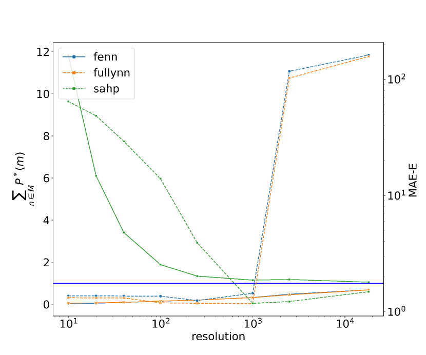
(a) Bookorder

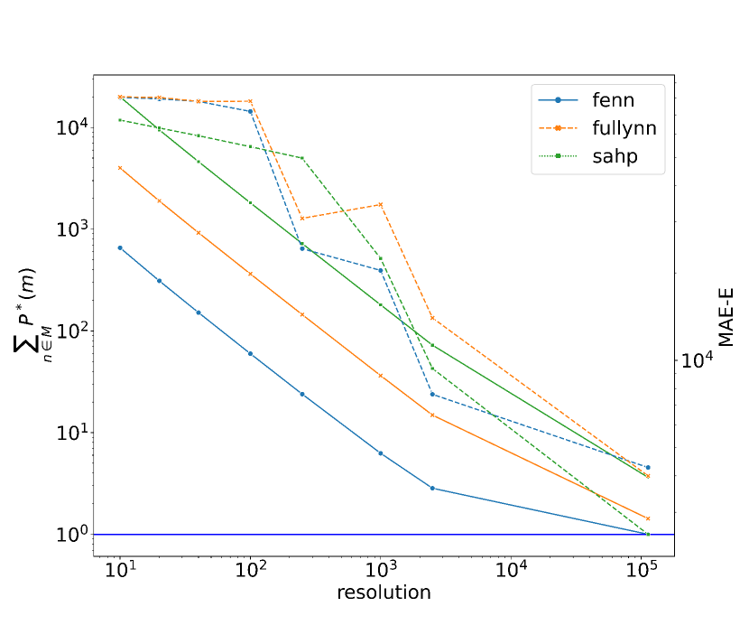
(b) Retweet

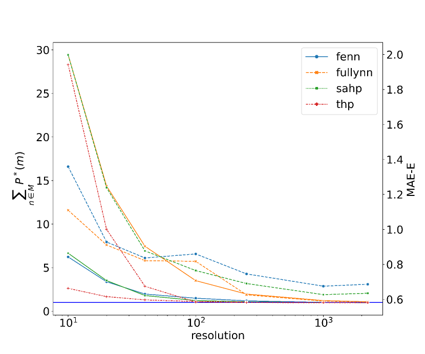
(c) StackOverflow

Figure 6: The value of $\sum_{\mathrm{M}}{P^{*}(m)}$ with different numbers of sampling points. The graph on MOOC is unavailable because of memory issues. The blue line is $y=1$. Solid lines refer to the sum of $P^{*}(m)$, and dashed lines refer to the MAE-E value with the corresponding sampling rate. These three graphs prove that we need plenty of sampling points for calculating every $P^{*}(m)$, and more accurate $P^{*}(m)$ could often result in sensible time predictions for event-time prediction tasks.

One could notice that in Figure 6, FullyNN and FENN give poor time predictions on Bookorder when the number of sampling points is bigger and $\sum_{\mathrm{M}}{P^{*}(m)}$ is closer to 1. After investigating the learning distribution over time, we find these two models might overfit the training set. Such overfitting introduces super high (over 200) yet narrow (around 0.01) spikes into the intensity function, which can only catch with a huge sampling rate. Such spikes severely damage the time prediction performance of FENN and FullyNN on Bookorder. This problem further proves the superiority of the IFIB framework.

Appendix H IFIB-C Result Visualization

We visualize the comparison between predicted $\hat{p}^{*}(m,t)$ using IFIB-C and the ground truth probability distributions $p^{*}(m,t)$ on synthetic dataset, Hawkes_1, in Figure 7(a). The Spearman coefficient $\rho$ and $L^{1}$ distance between $\hat{p}^{*}(m,t)$ and $p^{*}(m,t)$ demonstrate the desirable performance of IFIB-C. We also visualize the predicted $\hat{p}^{*}(m,t)$ using IFIB-C in Figure 7(b). We can observe the consistency between $\hat{p}^{*}(m,t)$ and the occurrence frequency of events along with time.

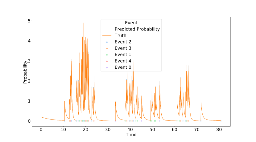
(a) Synthetic dataset - Hawkes_1 (Spearman coefficient $\rho=1.0000$, $L_{1}=0.1301$)

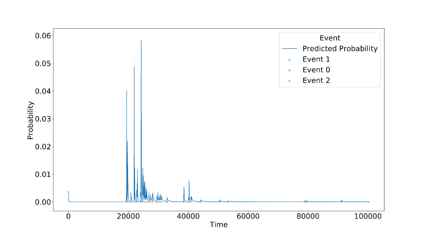
(b) Real-world dataset - Retweet

Figure 7: The comparison between the probability distribution learned by IFIB-C and the ground truth.

References

- Cao et al. [2017] Q. Cao, H. Shen, K. Cen, W. Ouyang, and X. Cheng. DeepHawkes: Bridging the Gap between Prediction and Understanding of Information Cascades. In E.-P. Lim, M. Winslett, M. Sanderson, A. W.-C. Fu, J. Sun, J. S. Culpepper, E. Lo, J. C. Ho, D. Donato, R. Agrawal, Y. Zheng, C. Castillo, A. Sun, V. S. Tseng, and C. Li, editors, Proceedings of the 2017 ACM on Conference on Information and Knowledge Management, CIKM 2017, Singapore, November 06 - 10, 2017, pages 1149–1158. ACM, 2017. doi: 10.1145/3132847.3132973.
- Charpentier et al. [2019] B. Charpentier, M. Bilos, and S. Günnemann. Uncertainty on Asynchronous Time Event Prediction. In H. M. Wallach, H. Larochelle, A. Beygelzimer, F. d’Alché Buc, E. B. Fox, and R. Garnett, editors, Advances in Neural Information Processing Systems 32: Annual Conference on Neural Information Processing Systems 2019, NeurIPS 2019, December 8-14, 2019, Vancouver, BC, Canada, pages 12831–12840, 2019.
- Chen et al. [2020] R. T. Q. Chen, B. Amos, and M. Nickel. Neural Spatio-Temporal Point Processes. In 9th International Conference on Learning Representations, ICLR 2021, Virtual Event, Austria, May 3-7, 2021, Sept. 2020. URL https://openreview.net/forum?id=XQQA6-So14.
- Daley and Vere-Jones [2003] D. J. Daley and D. Vere-Jones. An Introduction to the Theory of Point Processes. Springer, New York, 2 edition, 2003.
- Du et al. [2016] N. Du, H. Dai, R. Trivedi, U. Upadhyay, M. Gomez-Rodriguez, and L. Song. Recurrent Marked Temporal Point Processes: Embedding Event History to Vector. In Proceedings of the 22nd ACM SIGKDD International Conference on Knowledge Discovery and Data Mining, pages 1555–1564, New York, New York USA, 2016. ACM. doi: 10.1145/2939672.2939875.
- Enguehard et al. [2020] J. Enguehard, D. Busbridge, A. Bozson, C. Woodcock, and N. Hammerla. Neural Temporal Point Processes For Modelling Electronic Health Records. In Proceedings of the Machine Learning for Health NeurIPS Workshop, pages 85–113. PMLR, Nov. 2020. ISSN: 2640-3498.
- Guo et al. [2018] R. Guo, J. Li, and H. Liu. INITIATOR: Noise-contrastive Estimation for Marked Temporal Point Process. In J. Lang, editor, Proceedings of the Twenty-Seventh International Joint Conference on Artificial Intelligence, IJCAI 2018, July 13-19, 2018, Stockholm, Sweden, pages 2191–2197. ijcai.org, 2018. doi: 10.24963/ijcai.2018/303.
- HAWKES [1971] A. G. HAWKES. Spectra of some self-exciting and mutually exciting point processes. Biometrika, 58(1):83–90, 1971. ISSN 0006-3444. doi: 10.1093/biomet/58.1.83.
- Leskovec and Krevl [2014] J. Leskovec and A. Krevl. SNAP Datasets: Stanford large network dataset collection. http://snap.stanford.edu/data, June 2014.
- Mei and Eisner [2017] H. Mei and J. Eisner. The Neural Hawkes Process: A Neurally Self-Modulating Multivariate Point Process. In I. Guyon, U. v. Luxburg, S. Bengio, H. M. Wallach, R. Fergus, S. V. N. Vishwanathan, and R. Garnett, editors, Advances in Neural Information Processing Systems 30: Annual Conference on Neural Information Processing Systems 2017, December 4-9, 2017, Long Beach, CA, USA, pages 6754–6764, 2017.
- Mei et al. [2020] H. Mei, T. Wan, and J. Eisner. Noise-Contrastive Estimation for Multivariate Point Processes. In H. Larochelle, M. Ranzato, R. Hadsell, M. F. Balcan, and H. Lin, editors, Advances in Neural Information Processing Systems, volume 33, pages 5204–5214. Curran Associates, Inc., 2020.
- Ogata [1981] Y. Ogata. On Lewis’ simulation method for point processes. IEEE Transactions on Information Theory, 27(1):23–31, Jan. 1981. ISSN 1557-9654. doi: 10.1109/TIT.1981.1056305. Conference Name: IEEE Transactions on Information Theory.
- Omi et al. [2019] T. Omi, N. Ueda, and K. Aihara. Fully Neural Network based Model for General Temporal Point Processes. In H. M. Wallach, H. Larochelle, A. Beygelzimer, F. d’Alché Buc, E. B. Fox, and R. Garnett, editors, Advances in Neural Information Processing Systems 32: Annual Conference on Neural Information Processing Systems 2019, NeurIPS 2019, December 8-14, 2019, Vancouver, BC, Canada, pages 2120–2129, 2019.
- Rasmussen [2018] J. G. Rasmussen. Lecture Notes: Temporal Point Processes and the Conditional Intensity Function. arXiv:1806.00221, 2018.
- Salehi et al. [2019] F. Salehi, W. Trouleau, M. Grossglauser, and P. Thiran. Learning Hawkes Processes from a handful of events. In H. M. Wallach, H. Larochelle, A. Beygelzimer, F. d’Alché Buc, E. B. Fox, and R. Garnett, editors, Advances in Neural Information Processing Systems 32: Annual Conference on Neural Information Processing Systems 2019, NeurIPS 2019, December 8-14, 2019, Vancouver, BC, Canada, pages 12694–12704, 2019.
- Shchur et al. [2020] O. Shchur, M. Bilos, and S. Günnemann. Intensity-Free Learning of Temporal Point Processes. In 8th International Conference on Learning Representations, ICLR 2020, Addis Ababa, Ethiopia, April 26-30, 2020. OpenReview.net, 2020.
- Zhang et al. [2020] Q. Zhang, A. Lipani, O. Kirnap, and E. Yilmaz. Self-Attentive Hawkes Process. In Proceedings of the 37th International Conference on Machine Learning, pages 11183–11193. PMLR, Nov. 2020. ISSN: 2640-3498.
- Zhao et al. [2015] Q. Zhao, M. A. Erdogdu, H. Y. He, A. Rajaraman, and J. Leskovec. SEISMIC: A Self-Exciting Point Process Model for Predicting Tweet Popularity. In L. Cao, C. Zhang, T. Joachims, G. I. Webb, D. D. Margineantu, and G. Williams, editors, Proceedings of the 21th ACM SIGKDD International Conference on Knowledge Discovery and Data Mining, Sydney, NSW, Australia, August 10-13, 2015, pages 1513–1522. ACM, 2015. doi: 10.1145/2783258.2783401.
- Zuo et al. [2020] S. Zuo, H. Jiang, Z. Li, T. Zhao, and H. Zha. Transformer Hawkes Process. In Proceedings of the 37th International Conference on Machine Learning, pages 11692–11702. PMLR, Nov. 2020. ISSN: 2640-3498.