Stability and Generalization of Hypergraph Collaborative Networks

Abstract

Graph neural networks have been shown to be very effective in utilizing pairwise relationships across samples. Recently, there have been several successful proposals to generalize graph neural networks to hypergraph neural networks to exploit more complex relationships. In particular, the hypergraph collaborative networks yield superior results compared to other hypergraph neural networks for various semi-supervised learning tasks. The collaborative network can provide high quality vertex embeddings and hyperedge embeddings together by formulating them as a joint optimization problem and by using their consistency in reconstructing the given hypergraph. In this paper, we aim to establish the algorithmic stability of the core layer of the collaborative network and provide generalization guarantees. The analysis sheds light on the design of hypergraph filters in collaborative networks, for instance, how the data and hypergraph filters should be scaled to achieve uniform stability of the learning process. Some experimental results on real-world datasets are presented to illustrate the theory.

1 Introduction

Many real-world applications involve datasets that exhibit graph structures that depict pairwise relationships between vertices. These applications span a wide range of domains, including text analysis yao-mao-luo18 ; xu-etal:20 , social network analysis chen-li-bruna20 , molecule classification in chemistry gilmer-etal17 , point cloud processing te-etal18 , mesh generation litany-etal18 , and knowledge graphs rui-etal:22 , to name a few. In some applications, the only available data are graphs, while in some other applications, features about the vertices and edges are also available. Very naturally, machine learning algorithms that can exploit both graphs and features often yield better results than algorithms that solely rely on graph structures. Of particular interest is the class of graph convolution network (GCN) methods kipf-welling17 ; li-etal18 ; such-etal17 . These methods use neural network layers whose output at a vertex depends mostly on others that are deemed relevant according to the graph structure. A very common point of view is that GCN is a generalization of the traditional spatial filters, where graphs can represent neighbors that are not limited to spatial closeness.

While graphs can depict pairwise relationships, hypergraphs can represent relationships between multiple vertices. A hypergraph is a graph in which each edge, or hyperedge, can connect to multiple vertices. Hypergraphs can therefore represent more complex relationships. For example, in traditional paper-authorship networks, two articles (vertices) are connected if they share one or more coauthors. In this way, authorship information, which can provide important clues to the topic of the articles, is lost. Hypergraphs come to the rescue by treating each author as a hyperedge and each article as a vertex. Several works have been devoted to hypergraph learning. In zhou-huang-scholkopf06 , spectral clustering and semi-supervised parametric models on graphs were extended to hypergraphs. In gao-etal20 , a tensor representation of hypergraphs was proposed to make the optimization of hypergraphs more amenable. Generalizations of graph convolution networks to hypergraph convolution networks have been studied in feng-etal19 ; bai-zhang-torr21 ; dong-sawin-bengio20 ; yadati-etal19 . The main task is to define a convolution operator in a hypergraph such that the transition probability between two vertices can be measured, and the embeddings (or features) of each vertex can be propagated in a hypergraph convolution network. More propagations should be done between vertices connected by a common hyperedge.

Recently, wu-ng22 and wu-yan-ng22 studied and developed the convolution of vertex and hyperedge features to suitably aggregate values in hypergraphs. It was shown that such hypergraph collaborative networks (HCoN) have obtained superior results in some semi-supervised learning problems compared to other hypergraph neural network models. The proposal is to formulate the learning of vertex and hyperedge embeddings as a joint optimization problem to allow for updating the vertex and hyperedge embeddings simultaneously. The authors showed that the performance can be further boosted by incorporating a hypergraph reconstruction error as one of the objectives.

Apart from the development of machine learning algorithms and applications, efforts on the theory have also been made in the past decades, from general learning theory to specific properties of a class of algorithms. In this paper, we aim to study the algorithmic stability and generalization of the class of HCoN. We show that, in the single-layer case, the HCoN is algorithmically stable. As a result, the generalization gap (difference between training error and testing error) converges to zero as the size of the training set increases. We should explain the notions of training and testing in our context in Section 3.6 below. The analysis sheds light on the design of hypergraph filters in HCoNs, for instance, how the data and filters should be scaled to achieve the uniform stability of the learning process. Our generalization result is also valid for hypergraph convolution networks with the propagation of vertex embeddings only.

The rest of the paper is organized as follows. In Section 2, we review some works related to hypergraph neural networks and generalization guarantee studies. In Section 3, we introduce the HCoN model, some assumptions about the loss function and activation function, and some preliminary results. The results of the algorithmic stability of the HCoN and the generalization guarantee are established in Section 4. In Section 5, we present some experimental studies on the generalization gap to illustrate the theory. Some concluding remarks are given in Section 6.

2 Related Work

Generalization guarantees concern the expected difference between training and testing errors. Bousquet and Elisseeff bousquet-elisseeff02 and Mukherjee et al. mukherjee-etal06 showed that under suitable regularity assumptions, the stability of an algorithm implies generalization. In addition to the general theory, Bousquet and Elisseeff bousquet-elisseeff02 also studied the stability and generalization of the global minimizer of some regularized learning models. Such results are therefore independent of the particular algorithm used to compute an approximate optimizer. Stochastic gradient descent (SGD) is a popular algorithm to obtain a suboptimal solution to optimization problems. Some classical results on the generalization of SGD in the case of a single pass of data are reported in nemirovski-yudin83 . The analysis in the case of multiple passes of SGD is reported in hardt-recht-singer15 .

Stability and generalization analysis of SGD applied to graph convolution networks (GCNs) is studied in verma-zhang19 . The stability is established in terms of the dominant eigenvalue of the graph filter. A difference between verma-zhang19 and bousquet-elisseeff02 is that the former considers the model parameters computed via SGD, whereas the latter considers the theoretical optimal model parameters. Our work generalizes the analysis of GCNs in verma-zhang19 to hypergraph collaborative networks wu-ng22 ; wu-yan-ng22 which also include some edge features. A technical difference between our work and verma-zhang19 is that the latter assumes some Lipschitz conditions on the composition of the loss function and the neural network outputs but we require some Lipschtiz conditions on the loss function only. Ours are therefore easier to verify and more fundamental.

Various kinds of stability have been proposed and studied in the literature bousquet-elisseeff02 ; mukherjee-etal06 . Similar to verma-zhang19 , we use uniform stability which yields tighter bounds than other forms of stability, such as error stability, hypothesis stability and pointwise hypothesis stability bousquet-elisseeff02 . Finally, another related work is belkin-matveeva-niyogi04 , which studied regularized graph learning problems and devised some generalization guarantees. However, the resulting generalization gap is inversely proportional to the second smallest eigenvalue of the graph Laplacian matrix. Thus the bound can grow with the size of the graph. The bounds devised by us and verma-zhang19 are independent of the graph size, and the generalization gap converges to zero with the sample size and the graph size.

3 Hypergraph Convolution Networks

3.1 Hypergraphs

A hypergraph is a graph where a hyperedge can connect to any number of vertices. In the undirected version, each hyperedge is represented by a subset of vertices. A hypergraph is denoted by $\mathcal{G}=(\mathcal{V},\mathcal{E})$ where $\mathcal{V}$ is the set of vertices and $\mathcal{E}=\{e\;:\;e\subset\mathcal{V}\}$ is the set of hyperedges. The number of vertices and the number of hyperedges are denoted by $N=|\mathcal{V}|$ and $M=\rvert\mathcal{E}\rvert$, respectively. A hypergraph can also be represented by an incidence matrix $H\in\mathbb{R}^{N\times M}$, whose $(i,j)$-th equals $1$ if the $j$-th hyperedge is connected to the $i$-th vertex, and equals $0$ otherwise. For simplicity, we consider unweighted graphs, but the weights can be introduced into the hypergraph filters easily as done in feng-etal19 ; bai-zhang-torr21 ; dong-sawin-bengio20 ; yadati-etal19 .

Generalizations of graph convolution networks to hypergraph convolution networks have been studied. Given a feature matrix $X_{V}\in\mathbb{R}^{N\times F_{V}}$ (where $F_{V}$ is the dimension of the vertex features) and the dimension $O$ of the output embeddings, the convolution operator in a hypergraph for the propagation of vertex features (or embeddings) is constructed as follows:

$$f(X_{V}|Q_{V})=\sigma\left(D_{V}^{-\frac{1}{2}}HD_{E}^{-1}H^{\top}D_{V}^{-\frac{1}{2}}X_{V}Q_{V}\right),$$ (1)

where $\sigma(\cdot)$ is an activation function, $Q_{V}\in\mathbb{R}^{F_{V}\times O}$ is a matrix of learnable parameters, $H\in\mathbb{R}^{N\times M}$ is the incident matrix of the hypergraph, and $D_{V}=\mathrm{diag}(H\mathbf{1})$ and $D_{E}=\mathrm{diag}(H^{\top}\mathbf{1})$ are diagonal matrices with the degrees of the vertices and the degrees of the hyperedges on the diagonals. We note in (1) that the operator $D_{V}^{-\frac{1}{2}}HD_{E}^{-1}H^{\top}D_{V}^{-\frac{1}{2}}$ mixes the feature vectors of vertices connected by a common hyperedge. In this way, feature vectors of neighboring vertices of a vertex are propagated into the vertex and aggregated to form a new feature vector for the vertex. This model does not make use of hyperedge features.

3.2 The Hypergraph Collaborative Network Model

Unlike the hypergraph convolution networks in (1), the hypergraph collaborative networks (HCoN) in wu-ng22 and wu-yan-ng22 aim to predict vertex-level and hyperedge-level labels together based on the hypergraph structure and a set of vertex features and hyperedge features. The single-layer hypergraph collaborative network we consider is given by

$$f(X_{V},X_{E}|\theta) = \sigma\left(\tilde{H}\tilde{H}^{\top}X_{V}Q_{V}+\tilde{H}D_{E}^{-\frac{1}{2}}X_{E}Q_{E}\right)$$ (2)

$$g(X_{V},X_{E}|\theta) = \sigma\left(\tilde{H}^{\top}\tilde{H}X_{E}P_{E}+\tilde{H}^{\top}D_{V}^{-\frac{1}{2}}X_{V}P_{V}\right).$$ (3)

In addition to the notations in (1), here $X_{E}\in\mathbb{R}^{M\times F_{E}}$ is a given matrix of hyperedge features, $F_{E}$ is the dimension of the hyperedge features, $P_{V}\in\mathbb{R}^{F_{V}\times O}$, $Q_{E}\in\mathbb{R}^{F_{E}\times O}$ and $P_{E}\in\mathbb{R}^{F_{E}\times O}$ are the additional learnable parameters, $\theta=(Q_{V},Q_{E},P_{V},P_{E})$, and $\tilde{H}=D_{V}^{-\frac{1}{2}}HD_{E}^{-\frac{1}{2}}$ is the normalized incident matrix. The functions $f$ and $g$ are referred to as the vertex encoder and the hyperedge encoder, respectively. They are used to produce labels at vertices and hyperedges, respectively. In the sequel, we focus on the analysis of vertex encoder (2) because the analysis of (3) is essentially the same.

We remark that the HCoN model described in wu-yan-ng22 reads

$$f(X_{V},X_{E}|\theta) = \sigma\left(\alpha\tilde{H}W\tilde{H}^{\top}X_{V}Q_{V}+(1-\alpha)\tilde{H}WD_{E}^{-\frac{1}{2}}X_{E}Q_{E}\right)$$ (4)

$$g(X_{V},X_{E}|\theta) = \sigma\left(\beta\tilde{H}^{\top}U\tilde{H}X_{E}P_{E}+(1-\beta)\tilde{H}^{\top}UD_{V}^{-\frac{1}{2}}X_{V}P_{V}\right).$$ (5)

In this work, we assume that the vertex weights $W$ and hyperedge weights $U$ are set to identity matrices for ease of presentation. We also absorb the constants $\alpha$ and $\beta$ into the parameters $Q_{V}$, $Q_{E}$, $P_{V}$, and $P_{E}$; the degree of freedom of the model remains unchanged.

3.3 The Activation Function

Algorithmic stability concerns the change in the loss function value with respect to the change in the data. Since SGD aggregates gradients, it is very natural that the stability must rely on the regularity of the activation function and the loss function. The activation function $\sigma:\mathbb{R}\to\mathbb{R}$ is assumed to satisfy the following. Standard activations such as sigmoid, ELU, and tanh verify these assumptions. RELU fails the $\sigma$-smoothness. However, one can consider a smoothed RELU to restore the theory: $\sigma(x)=0$ if $x<-\epsilon$, $(x+\epsilon)^{2}/(2\epsilon)^{2}$ if $-\epsilon\leq x\leq\epsilon$, $x$ if $x>\epsilon$.

1. $\sigma$ continuous differentiable

2. $\sigma$-Lipschitz:

   $$|\sigma(x)-\sigma(y)|\leq\alpha_{\sigma}|x-y|\qquad\mbox{for all }x,y\in\mathbb{R}.$$ (6)

   It follows that the derivative $\sigma^{\prime}$ is bounded, i.e. $|\sigma^{\prime}(x)|\leq\alpha_{\sigma}$.

3. $\sigma$-smooth:

   $$|\sigma^{\prime}(x)-\sigma^{\prime}(y)|\leq\nu_{\sigma}|x-y|\qquad\mbox{for all }x,y\in\mathbb{R}.$$ (7)

3.4 The Loss Function

Let $\hat{y}$ be an estimated label and let $y$ be the true label. The loss function $\ell:[y_{\min},y_{\max}]\times[y_{\min},y_{\max}]\to\mathbb{R}^{+}$ is denoted by $\ell(\hat{y},y)$. The following assumptions are made.

1. Continuous w.r.t. $(\hat{y},y)$ and continuously differentiable w.r.t. $\hat{y}$

2. $\ell$-Lipschitz w.r.t. $\hat{y}$:

   $$\left|\ell(\hat{y},y)-\ell(\hat{y}^{\prime},y)\right|\leq\alpha_{\ell}|\hat{y}-\hat{y}^{\prime}|$$ (8)

   for all $\hat{y},\hat{y}^{\prime},y\in[y_{\min},y_{\max}]$. This implies that $|\frac{\partial\ell}{\partial\hat{y}}(\hat{y},y)|\leq\alpha_{\ell}$.

3. $\ell$-smooth w.r.t. $\hat{y}$:

   $$\left|\frac{\partial\ell}{\partial\hat{y}}(\hat{y},y)-\frac{\partial\ell}{\partial\hat{y}}(\hat{y}^{\prime},y)\right|\leq\nu_{\ell}|\hat{y}-\hat{y}^{\prime}|$$ (9)

   for all $\hat{y},\hat{y}^{\prime},y\in[y_{\min},y_{\max}]$.

By the nonnegativity and continuity of $\ell(\cdot,\cdot)$ and the compactness of $[y_{\min},y_{\max}]\times[y_{\min},y_{\max}]$, the loss function is bounded:

$$0\leq\ell(\hat{y},y)\leq\gamma_{\ell}\qquad\mbox{for all }\hat{y},y\in[y_{\min},y_{\max}].$$ (10)

In the case of the binary cross-entropy $\ell(\hat{y},y)=-y\ln\hat{y}$, the Lipschitzity condition does not hold. However, it can be easily remedied by rescaling or clipping $\hat{y}$ to the range of $[\epsilon,1]$ for a $0<\epsilon<1$, so that $\ell(\hat{y},y)\leq-\ln\epsilon$.

We remark that the following Lipschitzity of a composite function is assumed in verma-zhang19 :

$$\left\|\nabla_{\theta}[\ell(f(v|\theta),y)]-\nabla_{\theta}[\ell(f(v|\theta^{\prime}),y)]\right\|_{2} \leq \alpha_{\ell}\|\nabla_{\theta}f(v|\theta)-\nabla_{\theta}f(v|\theta^{\prime})\|_{2}.$$

Here, $\|\cdot\|_{2}$ denotes the Euclidean norm and $f(v|\theta)$ denotes the output of a neural network with parameters $\theta$ at vertex $v$. The $\theta$ and $\theta^{\prime}$ are two sets of parameters for the network. The $\nabla_{\theta}$ denotes the gradient operator w.r.t. $\theta$ (i.e. $\frac{\partial}{\partial\theta}$). Our assumption (9) is solely in terms of $\frac{\partial\ell}{\partial\hat{y}}$ and is more fundamental.

3.5 Network Outputs at a Single Vertex

In this subsection, we provide more details about the characteristics of the network outputs at each vertex and devise a bound of the hypergraph filter outputs that will be useful in the next section. We remark that a similar analysis can also be conducted for network outputs at each hyperedge. Here, we focus on the analysis of vertex propagation (2) only.

For a vertex $v\in\mathcal{V}$, let $\mathbf{e}(v)$ be a binary vector whose $j$-th entry is $1$ if $v$ is the $j$-th vertex and is $0$ otherwise. Denote the learnable parameters with $\theta=(Q_{V}^{\top},Q_{E}^{\top})^{\top}\in\mathbb{R}^{(F_{V}+F_{E})\times O}$. The output (2) for a vertex $v$ is given by

$$f(v|\theta) = \sigma\left(A_{v}Q_{V}+B_{v}Q_{E}\right)\in\mathbb{R}^{1\times O},$$

where $A_{v}:=\mathbf{e}(v)^{\top}\tilde{H}\tilde{H}^{\top}X_{V}$ and $B_{v}:=\mathbf{e}(v)^{\top}\tilde{H}D_{E}^{-\frac{1}{2}}X_{E}$. Note that $A_{v}$ is a linear combination of the vertex feature vectors over the neighboring vertices of $v$ and $B_{v}$ is a linear combination of the edge feature vectors over the hyperedges joining $v$. For notational simplicity, we assume that the output dimension is $O=1$ . The analysis also works for a general $O$ with minor modifications. Let

$$d_{v}=A_{v}Q_{V}+B_{v}Q_{E}.$$

Then, we have

$$f(v|\theta) = \sigma(d_{v})\in\mathbb{R}$$ (11)

$$\nabla_{\theta}f(v|\theta) = \sigma^{\prime}(d_{v})\left(A_{v}\;B_{v}\right)^{\top}\in\mathbb{R}^{(F_{V}+F_{E})\times 1}.$$ (12)

Here, $\nabla_{\theta}$ is the gradient operator w.r.t. $\theta$ and $\sigma^{\prime}$ is the derivative of $\sigma$.

Denote by $\|\cdot\|_{2}$ the matrix $2$-norm. Note that

$$\left\|\left(A_{v}\;B_{v}\right)\right\|_{2}^{2} = \left\|\mathbf{e}(v)^{\top}\tilde{H}\tilde{H}^{\top}X_{V}\right\|_{2}^{2}+\left\|\mathbf{e}(v)^{\top}\tilde{H}D_{E}^{-\frac{1}{2}}X_{E}\right\|_{2}^{2}$$

$$\leq \|X_{V}\|_{2}^{2}\|\tilde{H}\tilde{H}^{\top}\|_{2}^{2}+\|X_{E}\|_{2}^{2}\|\tilde{H}\|_{2}^{2}\|D_{E}^{-\frac{1}{2}}\|_{2}^{2}$$

$$\leq \|X_{V}\|_{2}^{2}\;\mu(\tilde{H})^{4}+\|X_{E}\|_{2}^{2}\;\mu(\tilde{H})^{2},$$

where $\mu(\tilde{H})=\|\tilde{H}\|_{2}$ is the largest singular value of $\tilde{H}$. The last inequality follows from the fact that the diagonal entries of $D_{E}$ are positive integers so that $\|D_{E}^{-\frac{1}{2}}\|_{2}\leq 1$. Let

$$g_{\max}:=\mu(\tilde{H})\sqrt{\|X_{V}\|_{2}^{2}\;\mu(\tilde{H})^{2}+\|X_{E}\|_{2}^{2}}.$$ (13)

It follows that

$$\left\|\left(A_{v}\;B_{v}\right)\right\|_{2}\leq g_{\max}.$$ (14)

Moreover, by (12) and (6), we have

$$\|\nabla_{\theta}f(v|\theta)\|_{2}\leq\alpha_{\sigma}g_{\max}.$$ (15)

Finally, we remark that if the two terms in the sum in (2) are weighted by $\alpha$ and $1-\alpha$ respectively as described in (4) and (5), then (14) and (15) hold with

$$g_{\max}:=\mu(\tilde{H})\sqrt{\alpha^{2}\|X_{V}\|_{2}^{2}\;\mu(\tilde{H})^{2}+(1-\alpha)^{2}\|X_{E}\|_{2}^{2}}.$$ (16)

3.6 The SGD Algorithm

Let $\mathcal{D}$ be an unknown joint distribution of the vertex and the associated label. Let

$$\mathcal{S}=\{(v_{1},y_{1}),(v_{2},y_{2}),\ldots,(v_{n},y_{n})\}$$

be a set of $n$ i.i.d. samples from $\mathcal{D}$. The set $\mathcal{S}$ serves as the training set for the HCoN. The objective function of an HCoN is given by

$$\mathcal{L}(\theta)=\frac{1}{n}\sum_{i=1}^{n}\ell(f(v_{i}|\theta),y_{i}).$$

The learning task is a transductive semi-supervised task. The incident matrix $H$ and the feature matrices $X_{V}$ and $X_{E}$ are considered given. The formation of a training set is a sampling of vertices (and the associated labels) in the network. The training process (or learning process) refers to the minimization of $\mathcal{L}$ via SGD. A testing sample is another i.i.d. sample of a vertex in the network. The testing process refers to taking the output at the testing sample and comparing it to the known label. The sample space is therefore a finite space, to which the concentration inequality we used below applies.

We consider $T$ iterations of the SGD algorithm, where the batch size is $1$. At the $t$-th iteration, a sample $(v_{i_{t}},y_{i_{t}})$ is drawn from $\mathcal{S}$ with replacement. The parameters $\theta=(Q_{V}^{\top},Q_{E}^{\top})^{\top}$ are updated as follows:

$$\theta_{t}=\theta_{t-1}-\eta\nabla_{\theta}\ell(f(v_{i_{t}}|\theta_{t-1}),y_{i_{t}})$$

for $t=1,2,\ldots,T$, where $\eta>0$ is the learning rate. The final parameters learnt are $\theta_{T}$, also denoted by $\theta(\mathcal{S},A)$. The variable $A$ denotes a particular randomization of SGD, i.e. the sequence $(i_{1},i_{2},\ldots,i_{T})$.

Let $\mathcal{S}^{\prime}=\{(v_{1}^{\prime},y_{1}^{\prime}),(v_{2}^{\prime},y_{2}^{\prime}),\ldots,(v_{n}^{\prime},y_{n}^{\prime})\}$ be a training set that differs from $\mathcal{S}$ with one sample. That is, for some $1\leq i^{*}\leq n$,

$$\left\{\begin{array}[]{ll}(v_{i}^{\prime},y_{i}^{\prime})=(v_{i},y_{i}),&\mbox{if }i\neq i^{*}\\ (v_{i}^{\prime},y_{i}^{\prime})\neq(v_{i},y_{i}),&\mbox{if }i=i^{*}.\end{array}\right.$$

Let $\theta^{\prime}=({Q_{V}^{\prime}}^{\top},{Q_{E}^{\prime}}^{\top})^{\top}$ be the parameters learned with $\mathcal{S}^{\prime}$. The SGD update is given by

$$\theta_{t}^{\prime}=\theta_{t-1}^{\prime}-\eta\nabla_{\theta}\ell(f(v_{i_{t}}^{\prime}|\theta_{t-1}^{\prime}),y_{i_{t}}^{\prime})$$

for $t=1,2,\ldots,T$. The initial parameters for $\mathcal{S}$ and $\mathcal{S}^{\prime}$ are set equal, i.e. $\theta_{0}=\theta_{0}^{\prime}$. The parameters learned, using the same randomization $A$ as that for $\mathcal{S}$, are denoted by $\theta_{T}^{\prime}=\theta^{\prime}(\mathcal{S}^{\prime},A)$.

The difference between the parameters $\theta_{t}$ and $\theta_{t}^{\prime}$ at the $t$-th SGD iteration is

$$\Delta\theta_{t}:=\theta_{t}-\theta_{t}^{\prime}=\left[\begin{array}[]{c}Q_{V,t}-Q_{V,t}^{\prime}\\ Q_{E,t}-Q_{E,t}^{\prime}\end{array}\right].$$

Since $\mathcal{S}$ and $\mathcal{S}^{\prime}$ are identical except for the $i^{*}$-th sample, if $t^{*}$ is the first iteration at which $(v_{i^{*}},y_{i^{*}})$ and $(v_{i^{*}}^{\prime},y_{i^{*}}^{\prime})$ are sampled, we have $\Delta\theta_{t}=0$ for all $t<t^{*}$. Note that

$$\Delta\theta_{t} = \Delta\theta_{t-1}-\eta\left[\nabla_{\theta}\ell(f(v_{i_{t}}|\theta_{t-1}),y_{i_{t}})-\nabla_{\theta}\ell(f(v_{i_{t}}^{\prime}|\theta_{t-1}^{\prime}),y_{i_{t}}^{\prime})\right].$$ (17)

4 Main Results

Following the approach of hardt-recht-singer15 and verma-zhang19 , we first establish the uniform stability of SGD and then obtain the generalization guarantees.

4.1 Uniform Stability

Recall that $\mathcal{S}$ and $\mathcal{S}^{\prime}$ are two training sets that differ only by the $i^{*}$-th sample. In Lemma 1 and Lemma 2, we bound the gradient difference when the same sample and different samples are used, respectively. Then, we devise the difference between the SGD updates for $\mathcal{S}$ and $\mathcal{S}^{\prime}$ in Lemma 3. The stability then follows in Theorem 4. Note that $\sigma^{\prime}$ is the derivative of $\sigma$. Other variables with a prime (^′) denote quantities derived from the perturbed training set $\mathcal{S}^{\prime}$.

Lemma 1.

At the $t$-th SGD iteration, we have

$$\left\|\nabla_{\theta}\ell(f(v|\theta_{t-1}),y)-\nabla_{\theta}\ell(f(v|\theta_{t-1}^{\prime}),y)\right\|_{2} \leq (\alpha_{\ell}\nu_{\sigma}+\nu_{\ell}\alpha_{\sigma}^{2})g_{\max}^{2}\|\Delta\theta_{t-1}\|_{2}.$$

Proof: Let $f=f(v|\theta_{t-1})$ and $f^{\prime}=f(v|\theta_{t-1}^{\prime})$. Let

$$d = A_{v}Q_{V,t-1}+B_{v}Q_{E,t-1}$$

$$d^{\prime} = A_{v}Q_{V,t-1}^{\prime}+B_{v}Q_{E,t-1}^{\prime}.$$

By (11) and (12), we have $f=\sigma(d)$, $f^{\prime}=\sigma(d^{\prime})$, and

$$\nabla_{\theta}f = \sigma^{\prime}(d)\left(A_{v}\;B_{v}\right)^{\top}$$

$$\nabla_{\theta}f^{\prime} = \sigma^{\prime}(d^{\prime})\left(A_{v}\;B_{v}\right)^{\top}.$$

Note that

$$d-d^{\prime}=\left(A_{v}\;B_{v}\right)\Delta\theta_{t-1}.$$

Therefore, by (14), we have

$$|d-d^{\prime}|\leq g_{\max}\|\Delta\theta_{t-1}\|_{2}.$$ (18)

Hence,

$$\left\|\nabla_{\theta}\ell(f,y)-\nabla_{\theta}\ell(f^{\prime},y)\right\|_{2} = \left\|\frac{\partial}{\partial\hat{y}}\ell(f,y)\nabla_{\theta}f-\frac{\partial}{\partial\hat{y}}\ell(f^{\prime},y)\nabla_{\theta}f^{\prime}\right\|_{2}$$

$$\leq \left\|\frac{\partial}{\partial\hat{y}}\ell(f,y)\nabla_{\theta}f-\frac{\partial}{\partial\hat{y}}\ell(f,y)\nabla_{\theta}f^{\prime}\right\|_{2}$$

$$+\left\|\frac{\partial}{\partial\hat{y}}\ell(f,y)\nabla_{\theta}f^{\prime}-\frac{\partial}{\partial\hat{y}}\ell(f^{\prime},y)\nabla_{\theta}f^{\prime}\right\|_{2}$$

$$= \left|\frac{\partial}{\partial\hat{y}}\ell(f,y)\right|\left|\sigma^{\prime}(d)-\sigma^{\prime}(d^{\prime})\right|\left\|\left(A_{v}\;B_{v}\right)\right\|_{2}$$

$$+\left|\frac{\partial}{\partial\hat{y}}\ell(f,y)-\frac{\partial}{\partial\hat{y}}\ell(f^{\prime},y)\right|\left|\sigma^{\prime}(d^{\prime})\right|\left\|\left(A_{v}\;B_{v}\right)\right\|_{2}$$

$$\leq \alpha_{\ell}\nu_{\sigma}|d-d^{\prime}|g_{\max}+\nu_{\ell}|f-f^{\prime}|\alpha_{\sigma}g_{\max}$$

$$\leq \alpha_{\ell}\nu_{\sigma}|d-d^{\prime}|g_{\max}+\nu_{\ell}\alpha_{\sigma}^{2}|d-d^{\prime}|g_{\max}$$

$$\leq (\alpha_{\ell}\nu_{\sigma}+\nu_{\ell}\alpha_{\sigma}^{2})g_{\max}^{2}\|\Delta\theta_{t-1}\|_{2}.$$

Lemma 2.

At the $t$-th SGD iteration, we have

$$\left\|\nabla_{\theta}\ell(f(v|\theta_{t-1}),y)-\nabla_{\theta}\ell(f(v^{\prime}|\theta_{t-1}^{\prime}),y^{\prime})\right\|_{2} \leq 2\alpha_{\ell}\alpha_{\sigma}g_{\max}.$$

Proof: Let $f=f(v|\theta_{t-1})$ and $f^{\prime}=f(v^{\prime}|\theta_{t-1}^{\prime})$. By (8) and (15), we have

$$\left\|\nabla_{\theta}\ell(f,y)-\nabla_{\theta}\ell(f^{\prime},y^{\prime})\right\|_{2} = \left\|\frac{\partial}{\partial\hat{y}}\ell(f,y)\nabla_{\theta}f-\frac{\partial}{\partial\hat{y}}\ell(f^{\prime},y^{\prime})\nabla_{\theta}f^{\prime}\right\|_{2}$$

$$\leq \left|\frac{\partial}{\partial\hat{y}}\ell(f,y)\right|\left\|\nabla_{\theta}f\right\|_{2}+\left|\frac{\partial}{\partial\hat{y}}\ell(f^{\prime},y^{\prime})\right|\left\|\nabla_{\theta}f^{\prime}\right\|_{2}$$

$$\leq 2\alpha_{\ell}\alpha_{\sigma}g_{\max}.$$

Lemma 3.

Let $\mathcal{S}$ and $\mathcal{S}^{\prime}$ be two training sets that differ by one sample. Let $\theta=\theta(\mathcal{S},A)$ and $\theta^{\prime}=\theta^{\prime}(\mathcal{S}^{\prime},A)$ be the graph filter parameters of the HCoN models trained using SGD for $T$ iterations on $\mathcal{S}$ and $\mathcal{S}^{\prime}$, respectively. Then, the expected difference in the filter parameters is bounded by,

$$\mathbb{E}_{A}[\|\Delta\theta_{T}\|_{2}]\leq\frac{\kappa_{0}}{n},$$

where

$$\kappa_{0}:=\frac{2\alpha_{\ell}\alpha_{\sigma}\left\{\left[1+\eta(\alpha_{\ell}\nu_{\sigma}+\nu_{\ell}\alpha_{\sigma}^{2})g_{\max}^{2}\right]^{T}-1\right\}}{(\alpha_{\ell}\nu_{\sigma}+\nu_{\ell}\alpha_{\sigma}^{2})g_{\max}}.$$

Proof: Let $1\leq t\leq T$ and let

$$\mathbf{h}=\nabla_{\theta}\ell(f(v|\theta_{t-1}),y)-\nabla_{\theta}\ell(f(v^{\prime}|\theta_{t-1}^{\prime}),y^{\prime}).$$

By (17), we have

$$\mathbb{E}_{A}[\|\Delta\theta_{t}\|_{2}] \leq \mathbb{E}_{A}[\|\Delta\theta_{t-1}\|_{2}]+\eta\mathbb{E}_{A}[\|\mathbf{h}\|_{2}].$$

Note that the probabilities of the two scenarios considered in Lemma 1 and Lemma 2 are $\frac{n-1}{n}$ and $\frac{1}{n}$, respectively. By Lemma 1 and Lemma 2, we have

$$\mathbb{E}_{A}[\|\mathbf{h}\|_{2}] \leq \frac{n-1}{n}\cdot\mathbb{E}_{A}[C\|\Delta\theta_{t-1}\|_{2}]+\frac{1}{n}\cdot\mathbb{E}_{A}[C^{\prime}]$$

$$\leq C\mathbb{E}_{A}[\|\Delta\theta_{t-1}\|_{2}]+\frac{1}{n}\cdot C^{\prime},$$

where $C:=(\alpha_{\ell}\nu_{\sigma}+\nu_{\ell}\alpha_{\sigma}^{2})g_{\max}^{2}$ and $C^{\prime}:=2\alpha_{\ell}\alpha_{\sigma}g_{\max}$. Hence, we have

$$\mathbb{E}_{A}[\|\Delta\theta_{t}\|_{2}] \leq (1+\eta C)\mathbb{E}_{A}[\|\Delta\theta_{t-1}\|_{2}]+\frac{\eta C^{\prime}}{n}.$$

Solving the above recursion with the initial condition $\Delta\theta_{0}=0$ yields

$$\mathbb{E}_{A}[\|\Delta\theta_{T}\|_{2}] \leq \frac{\eta C^{\prime}}{n}\cdot\frac{(1+\eta C)^{T}-1}{\eta C}=\frac{\kappa_{0}}{n}.$$

Next, we prove the uniform stability of the single-layer HCoN model trained using the SGD algorithm. Uniform stability has been introduced in bousquet-elisseeff02 for the study of nonrandomized algorithms, where the algorithms are assumed to be insensitive to the order of the training set. However, SGD is a randomized algorithm that depends on the order of the random samples. In hardt-recht-singer15 , the notion of uniform stability was extended to randomized algorithms. A randomized algorithm is said to be uniformly stable if there exists a constant $\beta$, possibly depending on $n$, such that

$$\sup_{\mathcal{S},\mathcal{S}^{\prime},v,y}|\mathbb{E}_{A}[\ell(f(v|\theta),y)-\ell(f(v|\theta^{\prime}),y)]|\leq\beta.$$

Here, $\theta=\theta(\mathcal{S},A)$ and $\theta^{\prime}=\theta^{\prime}(\mathcal{S}^{\prime},A)$ are the parameters learned with the datasets $\mathcal{S}$ and $\mathcal{S}^{\prime}$, respectively. Thus the difference in the loss function values is averaged over all randomizations. In this paper, we adopt this notion of uniform stability to establish a bound of the generalization gap.

Theorem 4 (Uniform Stability).

The single-layer HCoN model trained using the SGD algorithm for $T$ iterations is uniformly stable:

$$\sup_{\mathcal{S},\mathcal{S}^{\prime},v,y}|\mathbb{E}_{A}[\ell(f(v|\theta),y)-\ell(f(v|\theta^{\prime}),y)]|\leq\frac{\kappa}{n},$$

where

$$\kappa := \alpha_{\ell}\alpha_{\sigma}g_{\max}\kappa_{0}$$ (19)

$$= \frac{2\alpha_{\ell}^{2}\alpha_{\sigma}^{2}\left\{\left[1+\eta(\alpha_{\ell}\nu_{\sigma}+\nu_{\ell}\alpha_{\sigma}^{2})g_{\max}^{2}\right]^{T}-1\right\}}{\alpha_{\ell}\nu_{\sigma}+\nu_{\ell}\alpha_{\sigma}^{2}}.$$

Proof: Let $f=f(v|\theta)$ and $f^{\prime}=f(v|\theta^{\prime})$. By (11), we have $f=\sigma(d)$ and $f^{\prime}=\sigma(d^{\prime})$, where

$$d = A_{v}Q_{V}+B_{v}Q_{E}$$

$$d^{\prime} = A_{v}Q_{V}^{\prime}+B_{v}Q_{E}^{\prime}.$$

Hence, by (8), (6), (18) and Lemma 3, we have

$$\left|\mathbb{E}_{A}\left[\ell(f(v|\theta),y)-\ell(f(v|\theta^{\prime}),y)\right]\right| \leq \mathbb{E}_{A}\left[\left|\ell(f(v|\theta),y)-\ell(f(v|\theta^{\prime}),y)\right|\right]$$

$$\leq \alpha_{\ell}\mathbb{E}_{A}\left[\left|f(v|\theta)-f(v|\theta^{\prime})\right|\right]$$

$$\leq \alpha_{\ell}\alpha_{\sigma}\mathbb{E}_{A}\left[\left|d-d^{\prime}\right|\right]$$

$$\leq \alpha_{\ell}\alpha_{\sigma}g_{\max}\mathbb{E}_{A}\left[\left\|\Delta\theta_{T}\right\|_{2}\right]$$

$$\leq \alpha_{\ell}\alpha_{\sigma}g_{\max}\cdot\frac{\kappa_{0}}{n}=\frac{\kappa}{n}.$$

4.2 Generalization Gap

Consider an HCoN trained on $\mathcal{S}$ with a randomization $A$. Denote the output of the trained network by $f(v|\theta(\mathcal{S},A))$. Let $z=(v,y)$ be a random sample from $\mathcal{D}$. We denote the loss w.r.t. $z$ by

$$\ell(\mathcal{S},A,z):=\ell(f(v|\theta(\mathcal{S},A)),y).$$

The generalization error is defined by

$$R(\mathcal{S},A):=\mathbb{E}_{z}[\ell(\mathcal{S},A,z)].$$

The empirical risk (a.k.a. training error) is defined by:

$$R_{\mathrm{emp}}(\mathcal{S},A):=\frac{1}{n}\sum_{i=1}^{n}\ell(\mathcal{S},A,z_{i}),$$

where $z_{i}=(v_{i},y_{i})$ is the $i$-th sample in $\mathcal{S}$. The generalization gap is given by

$$G(\mathcal{S})=\mathbb{E}_{A}[R(\mathcal{S},A)-R_{\mathrm{emp}}(\mathcal{S},A)].$$

Next, we present a perturbation result for $G$. It is a general result for stable algorithms. The proof can be found in the Appendix of verma-zhang19 . However, we also include the proof here for completeness and we have fixed a few minor typos of verma-zhang19 . Recall that by Theorem 4, we have the uniform stability

$$|\mathbb{E}_{A}[\ell(f(v|\theta),y)-\ell(f(v|\theta^{\prime}),y)]|\leq\frac{\kappa}{n}.$$

Lemma 5 (Gap perturbation).

Let $\mathcal{S}$ and $\mathcal{S}^{\prime}$ be two training sets that differ by their $i^{*}$-th samples. Then,

$$|G(\mathcal{S})-G(\mathcal{S}^{\prime})|\leq\frac{2\kappa+\gamma_{\ell}}{n}.$$

Here, $\kappa$ is given by (19) and $\gamma_{\ell}$ is the upper bound of $\ell$.

Proof: First, consider the perturbation of $R(\mathcal{S},A)$:

$$\left|\mathbb{E}_{A}\left[R(\mathcal{S},A)-R(\mathcal{S}^{\prime},A)\right]\right| = \left|\mathbb{E}_{A}\left[\mathbb{E}_{z}\left[\ell(\mathcal{S},A,z)-\ell(\mathcal{S}^{\prime},A,z)\right]\right]\right|$$

$$= \left|\mathbb{E}_{z}\left[\mathbb{E}_{A}\left[\ell(\mathcal{S},A,z)-\ell(\mathcal{S}^{\prime},A,z)\right]\right]\right|$$

$$\leq \mathbb{E}_{z}\left[\left|\mathbb{E}_{A}\left[\ell(\mathcal{S},A,z)-\ell(\mathcal{S}^{\prime},A,z)\right]\right|\right]\leq\frac{\kappa}{n}.$$

Second, consider the perturbation of $R_{\mathrm{emp}}(\mathcal{S},A)$:

$$\left|\mathbb{E}_{A}\left[R_{\mathrm{emp}}(\mathcal{S},A)-R_{\mathrm{emp}}(\mathcal{S}^{\prime},A)\right]\right| \leq \left|\frac{1}{n}\sum_{j\neq i^{*}}\mathbb{E}_{A}\left[\ell(\mathcal{S},A,z_{j})-\ell(\mathcal{S}^{\prime},A,z_{j})\right]\right|$$

$$+\left|\frac{1}{n}\mathbb{E}_{A}\left[\ell(\mathcal{S},A,z_{i^{*}})-\ell(\mathcal{S}^{\prime},A,z_{i^{*}}^{\prime})\right]\right|$$

$$\leq \frac{1}{n}\sum_{j\neq i^{*}}\left|\mathbb{E}_{A}\left[\ell(\mathcal{S},A,z_{j})-\ell(\mathcal{S}^{\prime},A,z_{j})\right]\right|$$

$$+\frac{1}{n}\mathbb{E}_{A}\left[\left|\ell(\mathcal{S},A,z_{i^{*}})-\ell(\mathcal{S}^{\prime},A,z_{i^{*}}^{\prime})\right|\right]$$

$$\leq \frac{n-1}{n}\cdot\frac{\kappa}{n}+\frac{\gamma_{\ell}}{n}\leq\frac{\kappa+\gamma_{\ell}}{n}.$$

Finally, we have

$$|G(\mathcal{S})-G(\mathcal{S}^{\prime})| \leq \left|\mathbb{E}_{A}\left[R(\mathcal{S},A)-R(\mathcal{S}^{\prime},A)\right]\right|+\left|\mathbb{E}_{A}\left[R_{\mathrm{emp}}(\mathcal{S},A)-R_{\mathrm{emp}}(\mathcal{S}^{\prime},A)\right]\right|,$$

so that the result follows.

For reference, we state the classical McDiarmid’s concentration inequality mcdiarmid89 , which provides the chance of an inequality with respect to a random training set.

Proposition 6 (McDiarmid’s concentration inequality).

If $F(\mathcal{S})=F(z_{1},z_{2},\ldots,z_{n})$ is a function of $n$ i.i.d. random variables that satisfies

$$|F(\mathcal{S})-F(\mathcal{S}^{\prime})|\leq c$$

for all $\mathcal{S}$ and $\mathcal{S}^{\prime}$ that differ by one coordinate, then, for any $\epsilon>0$, we have

$$P\left(F(\mathcal{S})\leq\mathbb{E}_{\mathcal{S}}[F(\mathcal{S})]+\epsilon\right)\geq 1-e^{-\frac{2\epsilon^{2}}{nc^{2}}}.$$

We are now in position to present our main result for the generalization gap.

Theorem 7 (Generalization Gap).

Consider a single-layer HCoN model trained on a dataset $\mathcal{S}$ using the SGD algorithm for $T$ iterations. The following expected generalization gap holds for all $0<\delta<1$, with probability at least $1-\delta$,

$$\mathbb{E}_{A}[R(\mathcal{S},A)-R_{emp}(\mathcal{S},A)]\leq\frac{\kappa}{n}+\frac{2\kappa+\gamma_{\ell}}{\sqrt{n}}\cdot\sqrt{\frac{\ln\frac{1}{\delta}}{2}}.$$

Here, $\kappa$ is given by (19) and $\gamma_{\ell}$ is the upper bound of $\ell$.

Proof: Let $F(\mathcal{S})=G(\mathcal{S})$ be the generalization gap. By Lemma 5 and McDiarmid’s concentration inequality, we have

$$P\left\{G(\mathcal{S})\leq\mathbb{E}_{\mathcal{S}}[G(\mathcal{S})]+\epsilon\right\}\geq 1-e^{-\frac{2\epsilon^{2}}{nc^{2}}},$$

where $c:=\frac{2\kappa+\gamma_{\ell}}{n}$. Let $\delta=e^{-\frac{2\epsilon^{2}}{nc^{2}}}$. Note that

$$\epsilon=c\sqrt{\frac{n\ln\frac{1}{\delta}}{2}}=\frac{2\kappa+\gamma_{\ell}}{\sqrt{n}}\cdot\sqrt{\frac{\ln\frac{1}{\delta}}{2}}.$$

Hence, the following holds with a probability of at least $1-\delta$:

$$\mathbb{E}_{A}[R(\mathcal{S},A)-R_{\mathrm{emp}}(\mathcal{S},A)] \leq \mathbb{E}_{\mathcal{S}}[G(\mathcal{S})]+\frac{2\kappa+\gamma_{\ell}}{\sqrt{n}}\cdot\sqrt{\frac{\ln\frac{1}{\delta}}{2}}.$$

It remains to be shown that $\mathbb{E}_{\mathcal{S}}[G(\mathcal{S})]\leq\kappa/n$. Note that

$$\mathbb{E}_{\mathcal{S}}[G(\mathcal{S})] = \mathbb{E}_{\mathcal{S}}[\mathbb{E}_{A}[R(\mathcal{S},A)-R_{\mathrm{emp}}(\mathcal{S},A)]]$$

$$= \mathbb{E}_{\mathcal{S}}[\mathbb{E}_{A}[\mathbb{E}_{z}[\ell(\mathcal{S},A,z)]]]-\frac{1}{n}\sum_{j=1}^{n}\mathbb{E}_{\mathcal{S}}[\mathbb{E}_{A}[\ell(\mathcal{S},A,z_{j})]]$$

$$= \mathbb{E}_{\mathcal{S},z}[\mathbb{E}_{A}[\ell(\mathcal{S},A,z)]]-\mathbb{E}_{\mathcal{S}}[\mathbb{E}_{A}[\ell(\mathcal{S},A,z_{i})]]$$

$$= \mathbb{E}_{\mathcal{S},z_{i}^{\prime}}[\mathbb{E}_{A}[\ell(\mathcal{S},A,z_{i}^{\prime})]]-\mathbb{E}_{\mathcal{S},z_{i}^{\prime}}[\mathbb{E}_{A}[\ell(\mathcal{S}^{\prime},A,z_{i}^{\prime})]]$$

$$\leq \mathbb{E}_{\mathcal{S},z_{i}^{\prime}}[|\mathbb{E}_{A}[\ell(\mathcal{S},A,z_{i}^{\prime})-\ell(\mathcal{S}^{\prime},A,z_{i}^{\prime})]|]\leq\mathbb{E}_{\mathcal{S},z_{i}^{\prime}}\left[\frac{\kappa}{n}\right]=\frac{\kappa}{n}.$$

The last inequality is due to Theorem 4.

Theorem 7 states that as $n\to\infty$, the gap converges to zero at the rate of $O(1/{\sqrt{n}})$, provided that $\kappa$ in (19) does not grow with $n$ and the network size ($M$ and $N$). It boils down to the requirement that the $g_{\max}$ given in (13) does not grow with $n$, $M$ and $N$. In general, $g_{\max}$ can grow with the size of the network. For example, if the entries of $X_{V}$ and $X_{E}$ are uniformly distributed on the interval $[0,1]$, then $\|X_{V}\|_{2}=O(\sqrt{NF_{V}})$ and $\|X_{E}\|_{2}=O(\sqrt{MF_{E}})$. We therefore normalize each column of $X_{V}$ to a unit vector. Thus, we have $\|X_{V}\|_{2}\leq\|X_{V}\|_{F}=\sqrt{F_{V}}$, which is a constant independent of the graph size. Here, $\|\cdot\|_{F}$ denotes the Frobenius norm. Likewise, we also normalize $X_{E}$ so that $\|X_{E}\|_{2}\leq\sqrt{F_{E}}$. Another factor that may affect the growth of $g_{\max}$ is the incidence matrix $H$. When $H$ is normalized to $\tilde{H}$, it can be shown that the dominant singular value $\mu(\tilde{H})$ is bounded above by $1$ (see wu-yan-ng22 ). In contrast, we have $\mu(H)=O(\sqrt{NM})$. With both kinds of normalization in place, we have

$$g_{\max}\leq\sqrt{F_{V}+F_{E}}=O(1),$$

a constant independent of the graph size. Likewise, $g_{\max}$ in (16) is bounded by $\sqrt{\alpha^{2}F_{V}+(1-\alpha)^{2}F_{E}}=O(1)$.

It is worthwhile to compare our results with some related works. In the study of stable algorithms in bousquet-elisseeff02 , the learnt model $\theta$ is assumed to be a global optimizer of the loss function, which is assumed to be convex. There are no SGD iterations. As such, the corresponding constant $\kappa$ is independent of $T$. However, the assumption of global optimality is impractical. The work in hardt-recht-singer15 considers regression models with $\theta_{1},\ldots,\theta_{T}$ generated with SGD. The constant $\kappa$ is shown to be $O(T)$. However, there are also some rather strong convexity assumptions in the model that are not applicable to neural networks with nonlinearities. The bound in verma-zhang19 for GCNs has the same kind of exponential dependence on $T$ as ours. This is due to the lack of convexity in the model. Moreover, SGD does not guarantee a monotonic reduction of the loss function even when the learning rate is coupled with a line search. Thus the situation encountered in verma-zhang19 and in this paper is more sophisticated but more practical. However, we manage to establish the convergence with respect to the size $n$ of the training set.

The result indicates the consistency between training and testing errors, which is important for the model to be useful. Of course, it relies on the well-known fundamental assumption that the training and testing sets are drawn from the same distribution. In Section 5, we will also numerically study the generalization gap with respect to different parameters.

In the paper by wu-ng22 and wu-yan-ng22 , vertex and hyperedge classification is studied. Experimental results on several benchmark datasets have shown that the performance of the hypergraph collaborative network is better than that of the baseline methods. Our theoretical results for the stability and generalization of hypergraph collaborative networks can further confirm their usefulness.

Finally, we would like to remark that our theoretical analysis is also valid for hypergraph convolution networks (HCNs) in (1), where propagation of embedding is done on vertices only. The HCoN model reduces to an HCN when the hyperedge feature matrix $X_{E}$ is set to the zero matrix and the hyperedge feature dimension $F_{E}$ is set to zero.

Corollary 8 (Generalization Gap).

Consider a single layer HCN model trained on a dataset $\mathcal{S}$ using the SGD algorithm for $T$ iterations. The following expected generalization gap holds for all $0<\delta<1$, with probability at least $1-\delta$,

$$\mathbb{E}_{A}[R(\mathcal{S},A)-R_{emp}(\mathcal{S},A)]\leq\frac{\kappa}{n}+\frac{2\kappa+\gamma_{\ell}}{\sqrt{n}}\cdot\sqrt{\frac{\ln\frac{1}{\delta}}{2}}.$$

Here, $\kappa$ is given by (19) and $\gamma_{\ell}$ is the upper bound of $\ell$.

5 Experiments

The purpose of this section is to numerically study the behavior of the generalization gap of HCoNs. We refer the reader to wu-yan-ng22 for the accuracy of the model.

5.1 Datasets

We use the widely used benchmark datasets of Citeseer citeseer , Cora cora and PubMed pubmed for evaluations. The three networks consist of $1498$, $16313$, and $3840$ vertices, respectively.

Citeseer and PubMed are cocitation datasets. In the hypergraph, each vertex represents a document. The set of citations of a document form a hyperedge. The vertex features for Citeseer and PubMed are the bag-of-words vector representations and the term frequency-inverse document frequency (TF-IDF), respectively. Cora is a coauthorship dataset. Each vertex represents a document and each hyperedge represents an author connecting to documents of the author. The vertex features are the TF-IDF vectors of the documents. A more detailed description of the feature vector generation process can be found in wu-yan-ng22 . In each of the three networks, $30\%$ of the vertices are used as the test set; $30\%$–$70\%$ of the vertices are used as the training set.

5.2 Effect of the Weight

Fig. 1 shows the generalization gap as a function of the size of the training set. The weight $\alpha$ in (4) and (5) is varied to see its effects. The gap values are the average of $10$ different randomizations to serve as a proxy for the expectation $\mathbb{E}_{A}[\cdot]$. As the size of the training set increases, the generalization gap decreases. This is predicted with our theory that the gap decreases as the size of the training set increases. For a fixed size of the training set, the gap is smaller as $\alpha$ increases; this indicates that for these datasets, the vertex features are more important for prediction than the hyperedge features.

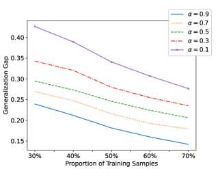
(a) Citeseer dataset

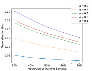
(b) Cora dataset

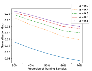
(c) PubMed dataset

Figure 1: Convergence of generalization gap as the training size $n$ increases.

5.3 Effect of the Learning Rate

Fig. 2 shows the generalization gap as a function of the size of the training set for different learning rates. The gap values are the average of $10$ different randomizations. The generalization gap reduces as the size of the training set $n$ increases. Moreover, the gap decreases with the learning rate for each fixed $n$. Such phenomena are consistent with the bound devised in Theorem 7.

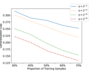
(a) Citeseer dataset

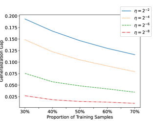
(b) Cora dataset

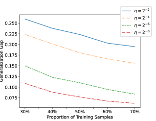
(c) PubMed dataset

Figure 2: Convergence of generalization gap as the training size $n$ increases.

To illustrate the convergence of the training process, we show the training and test loss function values at each epoch in Fig. 3. To avoid overwhelming with too many figures, we show only the result for $70\%$ training sample, $\alpha=0.9$ and $\eta=0.01$. The loss function values are the average of $10$ different randomizations. The graph shows that 1) the training loss function value is monotonically decreasing, and hence, the network fits better to the training data; 2) the test loss function value is also monotonically decreasing, and hence, the generalization error is improving. The starting training and test loss function values are similar because the network parameters are initialized randomly. The difference between the training and the test loss function values at the final epoch constitutes the generalization gap reported in Fig. 1 and Fig. 2. Our theory predicts that the gap at a fixed $T$ decreases as the size $n$ of the training set increases; see Fig. 1 and Fig. 2 for the convergence of the gap as a function of $n$.

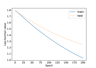
(a) Citeseer dataset

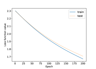
(b) Cora dataset

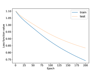
(c) PubMed dataset

Figure 3: Convergence of the training process as the number of iterations $T$ increases.

5.4 Effect of Incidence Matrix Normalization

In the experiment, we demonstrate the effect of normalization of the incidence matrix $H$. The normalized model is given in (4) and (5). The unnormalized model is obtained by replacing $\tilde{H}$ in (4) and (5) with $H$. Fig. 4 shows the generalization gap as the SGD progresses. The size of the training set is fixed to $70\%$. The $\alpha$ is fixed to $0.9$ because it yields the lowest gap and highest accuracy (see wu-yan-ng22 ). Each epoch represents a cycle of iterations over the whole training set. The gap values are obtained from a single randomization. First, the results show that when $H$ is normalized to $\tilde{H}$, the gap reaches a smaller level and converges faster as the number of iterations increases. This is predicted with our theoretical bound of the generalization gap since $\mu(\tilde{H})\leq 1$ whereas $\mu(H)=O(\sqrt{NM})$. The theory thus explains why normalization is important. Second, regarding the results with normalized incidence matrices, although the theoretical bound grows with $T$ (the number of iterations), the gap stabilizes quickly in practice. This is because the bound represents the worst-case scenario, which is pessimistic.

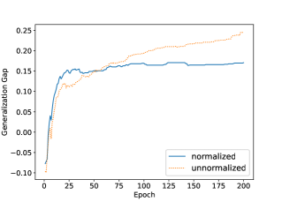
(a) Citeseer dataset

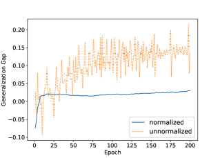
(b) Cora dataset

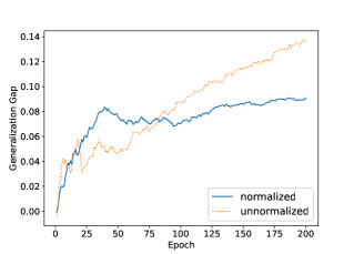
(c) PubMed dataset

Figure 4: Convergence of the generalization gap as the number of iterations $T$ increases.

6 Conclusion

In this paper, we have established uniform stability and generalization guarantee for single-layer hypergraph collaborative networks. The results show the importance of the the normalization of the vertex and hyperedge features and normalization of the hypergraph incidence matrix $H$. With these normalizations, we have a bound of the generalization gap independent of the graph size, and therefore, the generalization gap converges to zero. Some numerical experiments are presented to examine the convergence of the generalization gap in practice.

Several future research directions will be considered. 1) Extend the analysis to multilayer HCoNs, which are more useful in practice. The main challenge is that the gradients of the network become highly nonlinear and are more difficult to estimate. 2) Consider more general first-order stochastic optimization algorithms to include other commonly used algorithms such as SGD with momentum and ADAM. The problem is to devise estimates that can precisely reflect the potential acceleration delivered by these algorithms and study how the acceleration affects the stability and generalization gap. 3) While the present result has an advantage in that it does not assume any specific data distribution, it would also be useful to analyze the generalization gap in the presence of a data distribution. The idea is to improve the estimation of the expectations $\mathbb{E}_{z\sim\mathcal{D}}$ and $\mathbb{E}_{\mathcal{S}}$ in Lemma 5, Proposition 6, and Theorem 7. Specifically, determine the distribution of the gap from the assumed distribution of data, and the devise a special case of McDiarmid’s concentration inequality with an improved bound.

References

- \bibcommenthead
- (1) Yao, L., Mao, C., Luo, Y.: Graph convolutional networks for text classification (2018). https://arxiv.org/abs/1809.05679
- (2) Xu, H., Ma, Y., Liu, H., Deb, D., Liu, H., J., T., Jain, A.K.: Adversarial attacks and defenses in images, graphs and text: A review. International Journal of Automation and Computing 17, 151–178 (2020)
- (3) Chen, Z., Xiang Li, X., Bruna, J.: Supervised community detection with line graph neural networks (2020). https://arxiv.org/abs/1705.08415
- (4) Gilmer, J., Schoenholz, S.S., Riley, P.F., Vinyals, O., Dahl, G.E.: Neural message passing for quantum chemistry. In: Proceedings of the 34th International Conference on Machine Learning. 1263–1272, vol. 70. Sydney, Australia (2017)
- (5) Te, G., Hu, W., Guo, Z., Zheng, A.: RGCNN: Regularized graph CNN for point cloud segmentation (2018). https://arxiv.org/abs/1806.02952
- (6) Litany, O., Bronstein, A., Bronstein, M., Makadia, A.: Deformable shape completion with graph convolutional autoencoders. In: Proceedings of the IEEE Conference on Computer Vision and Pattern Recognition, Salt Lake City, UT, USA, pp. 1886–1895 (2018)
- (7) Rui, Y., Carmona, V.I.S., Pourvali, M., Xing, Y., Yi, W., Ruan, H., Zhang, Y.: Knowledge mining: A crross-disciplinary survey. Machine Intelligence Research 19(2), 89–114 (2022)
- (8) Kipf, T.N., Welling, M.: Semi-supervised classification with graph convolutional networks. In: 5th International Conference on Learning Representations, Toulon, France (2017). https://openreview.net/forum?id=SJU4ayYgl
- (9) Li, R., Wang, S., Zhu, F., Huang, J.: Adaptive graph convolutional neural networks (2018). https://arxiv.org/abs/1801.03226
- (10) Such, F.P., Sah, S., Dominguez, M.A., Pillai, S., Zhang, C., Michael, A., Cahill, N.D., Ptucha, R.: Robust spatial filtering with graph convolutional neural networks. IEEE Journal of Selected Topics in Signal Processing 11(6), 884–896 (2017)
- (11) Zhou, D., Huang, J., Schölkopf, B.: Learning with hypergraphs: Clustering, classification, and embedding. Neural Information Processing Systems 19, 1601–1608 (2006)
- (12) Gao, Y., Zhang, Z., Lin, H., Zhao, X., Du, S., Zou, C.: Hypergraph learning: Methods and practices. IEEE Transactions on Pattern Analysis and Machine Intelligence 44(5), 2548–2566 (2020)
- (13) Feng, Y., You, H., Zhang, Z., Ji, R., Gao, Y.: Hypergraph neural networks. In: Proceedings of the AAAI Conference on Artificial Intelligence, vol. 33, pp. 3558–3565 (2019)
- (14) Bai, S., Zhang, F., Torr, P.H.: Hypergraph convolution and hypergraph attention. Pattern Recognition 110, 107637 (2021)
- (15) Dong, Y., Sawin, W., Bengio, Y.: HNHN: Hypergraph networks with hyperedge neurons. In: Graph Representations and Beyond Workshop at International Conference on Machine Learning (2020)
- (16) Yadati, N., Nimishakavi, M., Yadav, P., Nitin, V., Louis, A., Talukdar, P.: HyperGCN: A new method of training graph convolutional networks on hypergraphs. In: Proceedings of the 33rd International Conference on Neural Information Processing Systems, vol. 135, pp. 1511–1522 (2019)
- (17) Wu, H., Ng, M.K.: Hypergraph convolution on nodes-hyperedges network for semi-supervised node classification. ACM Transactions on Knowledge Discovery from Data 46(4), 80–119 (2022)
- (18) Wu, H., Yan, Y., Ng, M.K.: Hypergraph collaborative network on vertices and hyperedges. IEEE Transactions on Pattern Analysis and Machine Intelligence (2022). Accepted for publication
- (19) Bousquet, O., Elisseeff, A.: Stability and generalization. Journal of Machine Learning Research 2, 499–526 (2002)
- (20) Mukherjee, S., Niyogi, P., Poggio, T., Rifkin, R.: Learning theory: Stability is sufficient for generalization and necessary and sufficient for consistency of empirical risk minimization. Advances in Computational Mathematics 25, 161–193 (2006)
- (21) Nemirovski, A., Yudin, D.B.: Problem Complexity and Method Efficiency in Optimization. Wiley Interscience, New York (1983)
- (22) Hardt, M., Recht, B., Singer, Y.: Train faster, generalize better: Stability of stochastic gradient descent (2015). https://arxiv.org/abs/1509.01240
- (23) Verma, S., Zhang, Z.: Stability and generalization of graph convolutional neural networks. In: 25th ACM SIGKDD International Conference on Knowledge Discovery and Data Mining (KDD 2019), Anchorage, AK, USA, pp. 1539–1548 (2019)
- (24) Belkin, M., Matveeva, I., Niyogi, P.: Regularization and semisupervised learning on large graphs. In: International Conference on Computational Learning Theory, pp. 624–638. Springer, Banff, Canada (2004)
- (25) McDiarmid, C.: On the method of bounded differences. Surveys in Combinatorics, pp. 148–188. Cambridge University Press, Cambridge (1989)
- (26) Bhattacharya, I., Getoor, L.: Collective entity resolution in relational data. ACM Transactions on Knowledge Discovery from Data 1(1), 5 (2007)
- (27) Sen, P., Namata, G., Bilgic, M., Getoor, L., Galligher, B., Eliassi-Rad, T.: Collective classification in network data. AI Magazine 29(3), 93 (2008)
- (28) Namata, G., London, B., Getoor, L., Huang, B.: Query-driven active surveying for collective classification. In: Proceedings of the Workshop on Mining and Learning with Graphs, vol. 8. Edinburgh, Scotland, UK (2012)