Evidence of Scaling Advantage for the Quantum Approximate
Optimization Algorithm on a Classically Intractable Problem

Abstract

The quantum approximate optimization algorithm (QAOA) is a leading candidate algorithm for solving optimization problems on quantum computers. However, the potential of QAOA to tackle classically intractable problems remains unclear. In this paper, we perform an extensive numerical investigation of QAOA on the Low Autocorrelation Binary Sequences (LABS) problem. The rapid growth of the problem’s complexity with the number of spins $N$ makes it classically intractable even for moderately sized instances, with the best-known heuristics observed to fail to find a good solution for problems with $N\gtrapprox 200$. We perform noiseless simulations with up to 40 qubits and observe that out to this system size, the runtime of QAOA with fixed parameters and a constant number of layers scales better than branch-and-bound solvers, which are the state-of-the-art exact solvers for LABS. The combination of QAOA with quantum minimum-finding on an idealized quantum computer gives the best empirical scaling of any algorithm for the LABS problem. We demonstrate experimental progress in compiling and executing QAOA for the LABS problem using an algorithm-specific error detection scheme on Quantinuum trapped-ion processors. Our results provide evidence for the utility of QAOA as an algorithmic component when executed on an idealized quantum computer.

Introduction

Quantum computers have been shown to have the potential to speed up the solution of optimization problems. At the same time, only a small number of algorithmic primitives are known that provide broadly applicable speedups. These include amplitude amplification Christoph Dürr and Peter Høyer (1996); Chakrabarti et al. (2022) and quantum walks more generally, Somma et al. (2008); Wocjan and Abeyesinghe (2008) as well as the recently introduced short path algorithm.Hastings (2018); Dalzell et al. (2023)

The dearth of provable speedups in quantum optimization motivates the development of heuristics. A leading candidate for demonstrating a heuristic speedup in quantum optimization is the quantum approximate optimization algorithm (QAOA).Hogg and Portnov (2000); Farhi et al. (2014) QAOA uses two operators applied in alternation $p$ times to prepare a quantum state such that, upon measuring it, a high-quality solution to the problem is obtained with high probability. A pair of such operators is commonly referred to as one QAOA “layer.” The state is evolved with a diagonal Hamiltonian encoding the optimization problem by the first operator and with a non-diagonal transverse-field Hamiltonian by the second operator. In this work, we consider the evolution times to be hyperparameters that are set by using a fixed, predetermined rule, analogously to the choice of a schedule in simulated annealing.

While QAOA has been studied extensively, Zhou et al. (2020); Basso et al. (2022); Boulebnane and Montanaro (2022); Sureshbabu et al. (2023) little is known about its potential to provide a scaling advantage over classical solvers. A recent numerical study Boulebnane and Montanaro (2022) of random $k$-SAT with $N\leq 20$ variables has shown that the time-to-solution (TTS) of QAOA with fixed parameters and constant depth grows as $1.23^{N}$. When QAOA is combined with amplitude amplification, the quantum TTS grows as $1.11^{N}$,Boulebnane and Montanaro (2022) whereas the best classical heuristic has TTS that grows as $1.25^{N}$.Boulebnane and Montanaro (2022) Our work is motivated by this preliminary numerical evidence on small instances, which indicates that QAOA may potentially scale better than classical solvers when executed on an idealized quantum computer.

We study the scaling of QAOA TTS with the problem size on the Low Autocorrelation Binary Sequences (LABS) problem,Boehmer (1967); Schroeder (1970) also known as the Bernasconi model in statistical physics.Bernasconi (1987); Mertens and Bessenrodt (1998) The LABS problem has applications in communications engineering, where the low autocorrelation sequences are used for designing radar pulses.Boehmer (1967); Golay (1977) To solve LABS, one has to produce a sequence of $N$ bits that minimizes a specific quartic objective.

We choose LABS to study the scaling of QAOA TTS for the following three reasons. First, the complexity of LABS grows rapidly, with optimal solutions known only for $N\leq 66$ and the best heuristics producing approximate solutions of quality decaying with $N$ for $N\gtrapprox 200$. Bošković et al. (2016); Packebusch and Mertens (2016) This makes it a promising candidate problem, since only a few hundred qubits are required to tackle classically intractable instances. Second, the performance of classical solvers for LABS has been benchmarked Bošković et al. (2016); Packebusch and Mertens (2016) in terms of the scaling of their TTS with problem size. We reproduce these results and observe that that the scaling of classical solvers at $N\leq 40$ matches the behavior at large $N$ reported in the literature. This provides evidence that the scaling we observe for QAOA at $N\leq 40$ will similarly extrapolate to large $N$. Third, LABS has only one instance per problem size $N$. Combined with the hardness of LABS, this makes it possible to reliably study the scaling of QAOA at large problem sizes, where simulating tens or hundreds of random instances would be computationally infeasible.

We obtain the scaling by performing noiseless exact simulation of QAOA with fixed schedules. Our results are enabled by a custom algorithm-specific GPU simulator,Lykov et al. which we execute using up to 1,024 GPUs per simulation on the Polaris supercomputer accessed through the Argonne Leadership Computing Facility. We find that the TTS of QAOA with number of layers $p=12$ grows as $1.46^{N}$, which is improved to $1.21^{N}$ if combined with quantum minimum-finding. This scaling is better than that of the best classical heuristic, which has a TTS that grows as $1.34^{N}$. We note that QAOA is a general quantum optimization heuristic with broad applicability, and no specific modifications have been done to adapt it to the LABS problem.

Our numerical evidence indicates that the proposed quantum algorithm scales better than the best classical heuristic in an idealized setting. However, we do not claim that QAOA is the best theoretically possible algorithm for the LABS problem. In particular, it may be possible to quadratically accelerate the best-known classical heuristic (Memetic Tabu Gallardo et al. (2009)) by applying ideas similar to those used in quantum simulated annealing. Somma et al. (2008); Lemieux et al. (2020); Boixo et al. (2015) Nonetheless, our results highlight the potential of QAOA to act as a useful algorithmic component that enables super-Grover quantum speedups.

As a first step toward execution of QAOA for the LABS problem, we implement QAOA on Quantinuum trapped-ion quantum processors Pino et al. (2021); Moses et al. (2023) on problems with up to $N=18$. We further implement an algorithm-specific error detection scheme inspired by Pauli error detection Gonzales et al. (2023); Debroy and Brown (2020) and demonstrate that it can reduce the impact of noise on solution quality by up to $65\%$. Our experiments highlight the continuing improvements to quantum computing hardware and the potential of algorithm-specific techniques to reduce the overhead of error detection and correction.

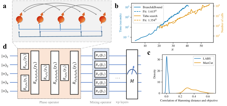
Figure 1: Classical and quantum algorithms applied to the LABS problem. a, Diagram of the LABS problem (with example of $N=5$). The problem involves non-local two-body (black lines) and four-body (blue lines) interactions. b, Time-to-solution (TTS) of classical solvers. For the sizes considered, we observe clear exponential scaling with exponents matching their asymptotic values reported in the literature (see Table 1). c, The distribution over $21\leq N\leq 31$ (for LABS) and $34$ random instances (for MaxCut on random 3-regular graphs with 20 nodes) of Pearson product-moment correlation coefficients relating the Hamming distance of bitstrings from the optimal solution with the objective value of the bitstring. LABS has a much lower correlation between the Hamming distance and objective, indicating that it is much harder than the commonly considered MaxCut problem. d, Diagram of QAOA circuit for a 5-qubit example. Starting from a uniform superposition of the computational basis states, we apply $p$ layers of phase and mixing operators, followed by measurement in the computational basis.

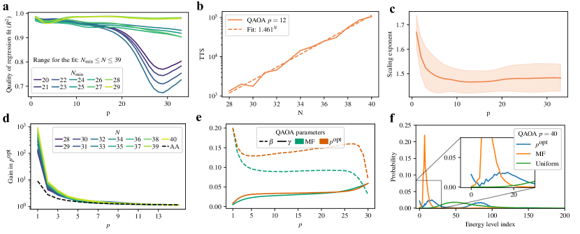
Figure 2: QAOA runtime scaling and dynamics under different parameter schedules. a, The quality of the exponential fit for different choices of minimum $N$ to include in the fit. $N\geq 28$ results in a robust fit, the quality of which does not deteriorate with $p$. $N=40$ is omitted as it was only simulated up to $p=22$. b, TTS of QAOA at $p=12$. Clear exponential scaling is observed. c, The scaling exponent of QAOA runtime for different QAOA depths $p$. Shaded area shows $95\%$ confidence interval. Increasing $p$ beyond $p\approx 12$ does not lead to better scaling. d, The gain in success probability $p^{\text{opt}}$ from applying step $p$ of QAOA and amplitude amplification (AA). The gain is defined as $p^{\text{opt}}_{\text{at step }p}/p^{\text{opt}}_{\text{at step }(p-1)}$. The gain at $p=1$ is over the random guess. Only one line is plotted for amplitude amplification since the lines for the values of $N$ considered are visually indistinguishable. For small $p$, a QAOA layer gives orders of magnitude larger gain than a step of AA. e, Fixed QAOA parameters for $p=30$ chosen with respect to the QAOA energy $\langle C\rangle_{\text{MF}}$ (“MF”) and probability of sampling the optimal solution (“$p^{\text{opt}}$”). Different choice of optimization objective gives different resulting parameters. f. Probability of obtaining a binary string corresponding to a given energy level of the LABS problem (the zeroth energy level is the ground state or optimal solution; lower is better). When parameters are optimized with respect to the expected merit factor (labeled “MF”), the QAOA output state is concentrated around the mean and fails to obtain a high overlap with the ground state. On the other hand, when parameters are optimized with respect to $p^{\text{opt}}$ (labeled “$p^{\text{opt}}$”), the QAOA state has a high overlap with both the ground state and higher energy states. The probability of obtaining the ground state is $27.3$ times greater for QAOA with parameters optimized with respect to $p^{\text{opt}}$ at $p=40$.

Problem statement

We begin by formally defining the LABS problem, discussing the state of the art of classical LABS solvers, and describing how QAOA is applied to solve the problem.

For a given sequence of spins $s_{i}\in\{\pm 1\}$, the autocorrelation is given as

$$\mathcal{A}_{k}(\bm{s})=\sum_{i=1}^{N-k}s_{i}s_{i+k}.$$ (1)

The goal of the LABS problem is to find a sequence of spins that minimizes the so-called “sidelobe” energy,

$$\mathcal{E}_{\text{sidelobe}}(\bm{s})=\sum_{k=1}^{N-1}\mathcal{A}_{k}^{2}(\bm{s}),$$ (2)

or, equivalently, maximizes the merit factor

$$\mathcal{F}(\bm{s})=\frac{N^{2}}{2\mathcal{E}_{\text{sidelobe}}(\bm{s})}.$$ (3)

The time-to-solution (TTS) is defined as the time a solver takes to produce this sequence. The energy $\mathcal{E}_{\text{sidelobe}}(\bm{s})$ is a polynomial containing terms of degree 2 and 4, visualized in Fig. 1a. It can be encoded on qubits by the following Hamiltonian:

$$H_{C}=2\sum_{i=1}^{N-3}\textsc{z}_{i} \sum_{t=1}^{\lfloor\frac{N-i-1}{2}\rfloor}\sum_{k=t+1}^{N-i-t}\textsc{z}_{i+t}\textsc{z}_{i+k}\textsc{z}_{i+k+t}$$ (4)

$$+\sum_{i=1}^{N-2}\textsc{z}_{i}\sum_{k=1}^{\lfloor\frac{N-i}{2}\rfloor}\textsc{z}_{i+2k},$$

where $\textsc{z}_{j}$ is a Pauli z operator acting on qubit $j$.

The runtimes of state-of-the-art classical solvers for the LABS problem scale exponentially, with clear exponential scaling present at $N\leq 40$ as shown in Fig. 1b. The best-known exact solvers are branch-and-bound methods that have a running time that scales as $1.73^{N}$.Packebusch and Mertens (2016) The best-known heuristic for general LABS is tabu search initialized with a memetic algorithm (Memetic Tabu) Gallardo et al. (2009), and has a running time that scales as $1.34^{N}$. Bošković et al. (2017)

To see why LABS is harder to solve than other commonly studied problems such as MaxCut, we can examine the correlation between the Hamming distance to the optimal solution and the objective. The comparison is shown in Fig. 1c. This correlation is one example of problem structure used by both classical and quantum heuristics to solve the problem quickly. Hogg and Portnov (2000) The absence of this correlation highlights the hardness of LABS compared with other commonly considered problems such as MaxCut.

As a consequence of the exponential scaling, the LABS problem becomes classically intractable at moderate sizes. Specifically, the value of the best-known merit factor decreases significantly for high $N$, whereas the asymptotic limit predicts that the merit factor should stay approximately constant. SOM This failure of state-of-the-art heuristics has been observed for $N>200$.Bošković et al. (2016); Packebusch and Mertens (2016) The clear failure of the classical method to obtain high-quality solutions even at small sizes makes LABS an appealing candidate problem for quantum optimization heuristics. SOM

In this work, we tackle the LABS problem using QAOA. As shown in the circuit diagram Fig. 1d, QAOA solves optimization problems by preparing a parameterized state

$$|\bm{\beta},\bm{\gamma}\rangle=\prod_{l=1}^{p}e^{-i\beta_{l}\sum_{j=1}^{N}\textsc{x}_{j}}e^{-i\gamma_{l}H_{C}}|+\rangle^{\otimes N},$$ (5)

where $|+\rangle^{\otimes N}$ is a uniform superposition over computational basis states, $H_{C}$ is the diagonal Hamiltonian encoding the problem, and $\textsc{x}_{j}$ is a Pauli x operator acting on qubit $j$. The operator $e^{-i\gamma H_{C}}$ is commonly referred to as the phase operator and $e^{-i\beta\sum_{j=1}^{N}\textsc{x}_{j}}$ as the mixing operator. The evolution times $\bm{\beta},\bm{\gamma}$ are hyperparameters chosen to maximize some figure of merit, such as the expected quality of the measurement outcomes or the probability of measuring the optimal solution. While $\bm{\beta},\bm{\gamma}$ can be optimized independently for each problem size, we consider them to be hyperparameters and use one fixed set of parameters for the LABS problem with a given QAOA depth $p$ regardless of size. The fixed set of parameters is obtained by optimizing $\bm{\beta},\bm{\gamma}$ numerically for a number of small problem sizes and introducing an averaging and rescaling procedure to extrapolate parameters to any problem size (see the Methods section).

When choosing the parameters $\bm{\beta},\bm{\gamma}$ and evaluating the quality of the solution obtained by QAOA, two figures of merit are commonly considered. The first one is the expected merit factor of the sampled binary strings, given by

$$\langle C\rangle_{\text{MF}}=\langle\bm{\beta},\bm{\gamma}|\frac{N^{2}}{2H_{C}}|\bm{\beta},\bm{\gamma}\rangle=\sum_{\bm{s}\in\{0,1\}^{N}}\mathsf{Pr}(\bm{s})\mathcal{F}(\bm{s}).$$ (6)

We will refer to $\langle C\rangle_{\text{MF}}$ as the “QAOA energy” as a shorthand. The second figure of merit is the probability of sampling the exact optimal solution, denoted by $p^{\text{opt}}$ and equal to the sum of squared absolute values of amplitudes of basis states corresponding to exactly optimal solutions.

In the numerical experiments below, we follow the protocol of Ref. Boulebnane and Montanaro, 2022 and focus on scaling of the QAOA TTS with problem size $N$ as the QAOA depth $p$ is held constant. QAOA TTS is defined as $\frac{1}{p^{\text{opt}}}$, i.e. the expected number of measurements required to obtain an optimal solution from the QAOA state. Ref. Boulebnane and Montanaro, 2022 rigorously shows that, for random $k$-SAT, the runtime of constant-depth QAOA grows exponentially with $N$ at any fixed $p$, with the scaling exponent depending on $p$. While the nature of the LABS problem makes it difficult to obtain analytical results analogous to Ref. Boulebnane and Montanaro, 2022, our numerical results also show clear exponential scaling of TTS. We note that, in practice, TTS of QAOA is $\Theta(N^{2})\frac{1}{p^{\text{opt}}}$, where the $\Theta(N^{2})$ prefactor comes from the cost of implementing the LABS phase oracle. Sanders et al. (2020) However, we do not include it in our analysis because it does not affect the scaling exponent.

Scaling of Quantum Time-to-Solution for LABS problem

We now present the numerical results demonstrating the scaling of TTS of QAOA and QAOA augmented with quantum minimum-finding (“QAOA$+$QMF”). The results are summarized in Table 1. Throughout this section, we present the numerical results obtained using exact noiseless simulations. The runtime scaling is obtained by evaluating QAOA once with fixed parameters $\bm{\beta},\bm{\gamma}$ (i.e., with no overhead of parameter optimization) and computing the value $p^{\text{opt}}$ with high precision. We discuss the parameter setting procedure and the details of simulation in the Methods section.

We are interested in the scaling of the runtime of QAOA for large problem sizes $N$. An important question to address is the choice of the smallest $N$ to include in the scaling analysis, since the algorithm’s behavior at small sizes may not be predictive of its behavior at large sizes. Note that the largest $N$ we include is limited by the capability of the classical simulator. We use the quality of the fit as the criterion for the choice of the cutoff on $N$. Figure 2a shows that if we set the cutoff at $N\geq 28$, we obtain a robust high-quality fit ($R^{2}>0.94$), with the quality of the fit remaining stable as $p$ grows. On the other hand, if smaller $N$ are included, the quality of fit begins to decay with $p$. Therefore we include only $N\geq 28$, obtaining the fit presented in Fig. 2b. We observe that TTS of QAOA grows as $1.46^{N}$ with problem size at constant QAOA depth $p=12$. We present evidence that the scaling exponent for QAOA at $p=12$ is not sensitive to the choice of $N_{\min}$ in Supplementary Information. SOM

	QAOA$+$QMF	QAOA	Memetic Tabu		Branch-and-bound
			Reproduced	Gallardo et al. (2009); Bošković et al. (2017)	Reproduced		TTO Packebusch and Mertens (2016)
					TTS	TTO
Fit	1.21	1.46	1.35	1.34	1.62	1.76	1.73
CI	(1.19, 1.23)	(1.42,1.50)	(1.33,1.38)	N/A	(1.57,1.66)	(1.72,1.79)	N/A

Table 1: Scaling exponents for quantum and classical algorithms. Confidence intervals (CIs) are $95\%$. The reported asymptotic exponential scaling of classical state-of-the-art solvers is reproduced at $N\leq 40$. For branch-and-bound, we include both the time to obtain a certificate of optimality (TTO reported in Ref. Packebusch and Mertens, 2016) as well as the much shorter time to find an optimal solution (TTS). We observe that QAOA with constant depth of $p=12$ augmented with quantum minimum-finding (“QAOA$+$QMF”) has better time-to-solution scaling than the best known classical heuristics.

As a quantum optimization heuristic with constant depth, on a fault-tolerant quantum computer the QAOA performance can be improved by using amplitude amplification Boulebnane and Montanaro (2022); Sanders et al. (2020) or, more specifically, quantum minimum-finding van Apeldoorn et al. (2020) (see Methods). The resulting scaling of TTS of QAOA augmented with quantum minimum-finding (“QAOA$+$QMF”) is $1.21^{N}$.

We observe that, beyond a certain value ($p\approx 12$), increasing QAOA depth does not lead to better scaling of TTS. This behavior is demonstrated in Fig. 2c. Consequently, running QAOA with $p$ higher than $12$ does not give any scaling advantage over amplitude amplification. This behavior is illustrated in Fig. 2d, which shows the increase in the success probability $p^{\text{opt}}$ from applying a given step of QAOA and amplitude amplification. For amplitude amplification, at step $p$ we have $p^{\text{opt}}=\left(\sin((2p+1)\arcsin{\sqrt{p_{0}}})\right)^{2}$, where $p_{0}=\frac{8}{2^{N}}$ is the initial (random guess) success probability. Boyer et al. (1998) Note that the $8$ in the numerator is a consequence of a dihedral group symmetry, namely, $D_{4}$. While asymptotically equivalent, amplitude amplification performs better than a realistic generalized minimum-finding algorithm, van Apeldoorn et al. (2020) as the formula used here considers the scenario where we know which states to amplify (i.e., the optimal merit factor is known). We observe that for small $p$, a step (layer) of QAOA gives orders of magnitude larger increase in success probability than does a step of amplitude amplification, implying an even larger improvement over direct application of quantum minimum-finding. We provide additional details on comparison between QAOA and amplitude amplification in the Supplementary Information. SOM

We observe that the QAOA dynamics with parameters optimized for expected solution quality $\langle C\rangle_{\text{MF}}$ and success probability $p^{\text{opt}}$ are different. We plot the optimized parameters in Fig. 2e. We note that the parameters optimized with respect to one metric give performance that is far from optimal with respect to the other metric. This can be seen in Fig. 2f, which plots the energy distribution (with respect to the cost Hamiltonian) of the states appearing in the QAOA wavefunction weighted by probability. With the parameters optimized for $\langle C\rangle_{\text{MF}}$, the QAOA output distribution is concentrated around its mean, and the overlap with the ground state or $p^{\text{opt}}$ is very small. On the other hand, when the parameters are optimized with respect to $p^{\text{opt}}$, the wavefunction is not concentrated and has large probability weight on the target ground state (i.e., high $p^{\text{opt}}$). This comes at the cost of significant overlap with high-energy states, which leads to poor expected solution quality. In the Supplementary Information SOM , we discuss the behavior of QAOA with parameters optimized with respect to different objectives.

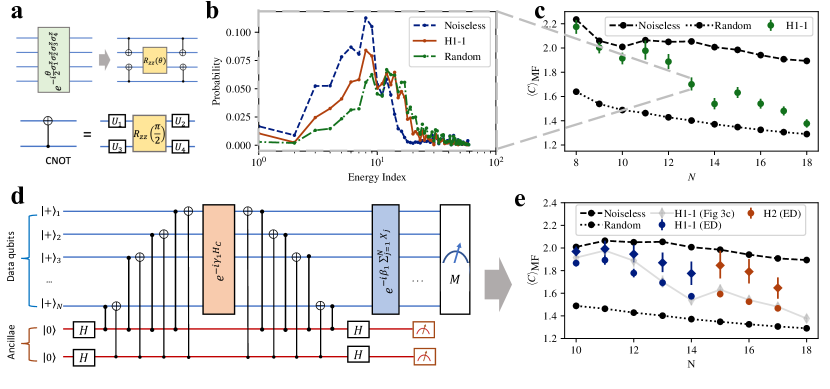
Figure 3: Experimental results on trapped-ion system. a, Decomposition of four-body interaction terms into a two-body $R_{\textsc{z}\textsc{z}}$ gate and four two-body cnot gates, which can be realized via native $R_{\textsc{z}\textsc{z}}$ gates. b, Energy density plot from experimental measured bitstrings for $N$=13. Energy index is arranged in energy ascending order. As a comparison, the distributions for noiseless $p=1$ QAOA simulation and random guess (assuming uniform distribution of all possible bitstrings) are shown. c, Experimental results up to 18 qubits on a trapped-ion quantum device (H1-1) with QAOA layer $p=1$ with optimized QAOA parameters. The error bars are calculated with 99% confidence intervals hereafter. d, Illustration of parity check circuit. The z and x parities of states are mapped to ancillary qubits after implementation of full (or part of) phase operators via cz and cnot gates, respectively, followed by mid-circuit measurement on the ancillary qubits to extract the parity syndrome result. e, Experimental results for circuit with parity check. Three mid-circuit z-parity and x-parity checks were performed using six ancillary qubits. The ancillae can also be reused after appropriate reset during the circuit. The red data points were run on the Quantinuum H2 hardware while the blue data were from the H1-1 device. Data run on the H1-1 device without any ancillary qubits are shown in grey. Circles (diamonds) are the data without (with) post-selection. The abbreviation ED refers to the error detection via the parity checks. Number of mid-circuit parity checks is fixed to be two for $N=10,11$ and three for all other $N$. Improvement in expected merit factor after post-selection according to parity syndrome measurement is observed.

Experiments on trapped-ion system

We now present the experimental results demonstrating the algorithmic and hardware progress toward the practical implementation of QAOA. Implementation of the phase operator is especially challenging for currently available quantum processors. It requires a large number of geometrically nonlocal two-qubit gates, demanding high gate fidelity.

Recent progress in trapped-ion platforms based on the QCCD architecture Moses et al. (2023); Pino et al. (2021); SOM has led to a rapid increase in the number of qubits while maintaining high fidelity, enabling large-scale QAOA demonstrations. Shaydulin and Pistoia (2023); He et al. (2023) These systems implement two-qubit gates between arbitrary pairs of qubits by transporting ions into physically separate gate zones, resulting in high-fidelity two-qubit gates with low crosstalk. We leverage this progress to execute QAOA circuits for the LABS problem on Quantinuum H-series trapped-ion systems.

To implement the QAOA circuit shown in Fig. 1d, we have to implement the phase operator. The four-body terms in the phase operator are decomposed into cnot gates and the native $R_{\textsc{z}\textsc{z}}(\theta)=e^{-i\frac{\theta}{2}\textsc{z}\textsc{z}}$ rotation as shown in Fig. 3a. To reduce the cost of implementing both the two-qubit and four-qubit interaction terms, we optimize the circuit by greedily canceling cnot gates (for algorithm details and gate count reduction see the Supplementary Information SOM ). The resulting circuit containing cnots and $R_{\textsc{z}\textsc{z}}$s is then transpiled into the two-qubit $R_{\textsc{z}\textsc{z}}$ gates and single-qubit gates that can be natively implemented by the trapped-ion system. SOM We remark that the number of two-qubit gates is $\approx 10^{3}$ at $N=18$, putting our experiments among the largest quantum optimization demonstrations on quantum hardware to date.Pelofske et al. (2023a, b); Niroula et al. (2022); He et al. (2023); Shaydulin and Pistoia (2023)

In this work we execute QAOA circuits with $p=1$ using parameters $\bm{\beta}$, $\bm{\gamma}$ optimized in noiseless simulation, followed by a projective measurement in the computational basis. In Fig. 3b, we show the energy probability distribution of measured bitstrings for $N=13$. We observe a broad distribution due to the limited number of layers and experimental imperfections. Nevertheless, even at high $N$, where two-qubit gate count is high and the gate errors can be significant, we observe a clear signal that indicates that QAOA is outperforming random guess. This is shown in Fig. 3c, which presents the experimentally obtained expected merit factors for various problem size up to $N=18$. We note that the merit factor drops quickly for larger $N$ and is approaching random guess because of experimental imperfections. We also note that at this scale LABS is easy for classical heuristics, which obtain optimal merit factors in $<1$ second. SOM Implementing QAOA for LABS instances that are hard for classical solvers would likely require error correction as the current implementation leads to an estimated two-qubit gate count of $\approx 7.5\times 10^{5}$ already at $N=67$ and $p=12$. SOM

To improve the performance in the presence of noise, we implement an algorithm-specific error detection scheme. Since only the phase operator requires two-qubit gates, we focus on detecting errors that occur in the corresponding part of the circuit. Our scheme is based on the Pauli sandwiching error-detecting procedure of Ref. Gonzales et al., 2023, which uses pairs of parity checks to detect some but not necessarily all errors that occur in a given part of the circuit. Following Refs. Shaydulin and Galda, 2021; Kakkar et al., 2022, we use the symmetries of the optimization problem to construct the parity checks. Specifically, we note that the LABS Hamiltonian preserves both z and x parities, that is, $[H_{C},\otimes_{i}^{N}\textsc{z}_{i}]=[H_{C},\otimes_{i}^{N}\textsc{x}_{i}]=0$. We compute the parities onto ancillary qubits and perform mid-circuit measurement to determine whether an odd number of z- or x-flip errors occur during the circuit execution. The circuit with one check is shown in Fig. 3d. In the hardware experiments shown in Fig. 3e, we use up to three parity checks and observe consistent improvements in QAOA performance after postselecting on their outcomes. After postselection, the difference of merit factor between experimental results and noiseless simulation is reduced by $54\%$ on average and up to $65\%$ for specific $N$. In the Supplementary Information SOM we present additional details on the error-detecting scheme performance, including how performance improves with the number of parity checks and the reduction in the algorithm runtime. We note that while error detection does not directly give samples with better merit factors, the potential improvement in runtime can be translated into performance gains at the algorithm level, for example by being able to take more samples within a given time budget. SOM In our experiments, in all but two cases the optimal bitstring could be found within the post-selected sample, and in all cases within the total sample. SOM

Discussion

Our main finding is that quantum minimum-finding enhanced with QAOA scales better than the best known classical heuristics for the LABS problem. This provides evidence for the potential of QAOA to act as a building block that provides algorithmic speedups on an idealized fault-tolerant quantum computer. We envision QAOA being used in a variety of algorithmic settings, similarly to how amplitude amplification acts as a subroutine in quantum algorithms for backtracking, branch-and-bound and so on.

We take the first step toward the execution of QAOA for the LABS problem by implementing an algorithm-specific error-detection scheme on a trapped-ion quantum processor. However, further improvements in quantum error correction and hardware are necessary to implement the quantum minimum-finding augmented with QAOA. In particular, the overheads of fault-toleranceBabbush et al. (2021) must be significantly reduced to realize the quantum speedup.

Methods

Quantum minimum-finding enhanced with QAOA

In this work, we present the scaling results for QAOA combined with amplitude amplification (AA), or, more specifically, with quantum minimum-finding (“QAOA$+$QMF” in Table 1). This reduces the scaling exponent by half as compared to directly sampling QAOA output. We now discuss in detail how QAOA is combined with the generalized quantum minimum-finding algorithm of Ref. van Apeldoorn et al., 2020 to obtain the stated scaling.

We begin by noting that standard AA is not sufficient. This is because the LABS problem is framed as optimization and not search, i.e. there is no oracle for marking a global minimum. The trick for handling optimization is to perform a standard reduction from optimization to feasibility. The reduction is performed by introducing a threshold on the cost as a constraint and performing a binary search using AA as a subroutine. The oracle used by AA marks the elements below the current threshold. This reduction was first introduced by Dürr and Høyer (DH). Christoph Dürr and Peter Høyer (1996) However, the quantum minimum-finding algorithm of Dürr and Høyer utilizes standard Grover search, i.e. it requires the initial state to be the uniform superposition. A modification to it is required to leverage the improved success probability afforded by QAOA.

Ref. van Apeldoorn et al., 2020 provided a simple extension of DH that allows arbitrary initial states, with the overall cost scaling inversely with overlap between the initial state and state encoding the optimal solution. We leverage this extension in our quantum algorithm. We use constant-depth QAOA to prepare the initial state for the quantum minimum-finding algorithm. As QAOA state has overlap with the optimal state that is much larger than that of uniform superposition SOM and scales more favorably, we obtain better performance than the direct minimum-finding of Dürr and Høyer. Specifically, we provide numerical evidence that our algorithm obtains a super-Grover speedup over exhaustive search for the LABS problem, and scales better than the best known classical heuristics. We present our modification to include QAOA for outputting an optimal solution $x^{*}$ to the LABS problem in Algorithm 1 below. It is based on the generalized minimum-finding procedure outlined in Lemma 48 of Ref. van Apeldoorn et al., 2020. To keep the current work self-contained, we include the analysis of the algorithm below. We will use the following standard quantum subroutine based on Grover search that searches for an element with unknown probability in a quantum state.

Lemma 1 (Exponential Quantum Search, Ref. Brassard et al., 2002).

Let $|\psi\rangle=U|0\rangle^{\otimes N}$ be a quantum state in a $2^{N}$-dimensional Hilbert space with computational basis elements indexed by $N$-bit bitstrings, and $m\colon\{0,1\}^{N}\to\{0,1\}$ be a marking function such that $\sum_{\{x|m(x)=1\}}|\langle\psi|x\rangle|^{2}\geq p$. There exists a quantum algorithm $\mathbf{EQSearch}(U,m,\delta)$ that outputs an element $x^{*}$ such that $m(x^{*})=1$ with probability at least $\delta$ using $O\left(\frac{1}{\sqrt{p}}\log\left(\frac{1}{\delta}\right)\right)$ applications of $U$ and $m$.

Algorithm 1 QAOA Enhanced with Quantum Minimum-Finding

Unitary $U_{\text{QAOA}}$ acting on $\mathbb{C}^{2^{N}}$ such that $\lvert\langle x^{*}|U_{\text{QAOA}}|0\rangle^{\otimes N}\rvert\geq 1/\sqrt{p_{\text{opt}}}$ for unknown $p_{\text{opt}}$, $V_{\text{LABS}}$ for computing $\mathcal{E}_{\text{sidelobe}}$ into a register, and $\delta\in(0,1)$, positive number $M\leq 2^{N}$, $C$ is the constant corresponding to the $O(\cdot)$ in Lemma 1

If $M$ is greater than $1/\sqrt{p_{\text{opt}}}$, output $x^{*}$ with $\geq 1-\delta$ probability using $O(\log(1/\delta)M)$ calls to $U_{\text{QAOA}}$ and $V_{\text{LABS}}$ (and their inverses).

$x_{\text{res}}$ is set to an empty list.

for $i\leftarrow 1$ to $\lceil\log(1/\delta)\rceil$ do

     $t\leftarrow 0$; $s_{0}\leftarrow\infty$

     while number of calls to $U_{\text{QAOA}}$ & $V_{\text{LABS}}$ is $<$ $3CMN$ do

         $t\leftarrow t+1$

         Define $m_{t}\colon\{0,1\}^{N}\to\{0,1\}$ such that $m_{t}(x)=1$ if and only if $\mathcal{E}_{\text{sidelobe}}(x)<s_{t-1}$. Note that $m_{t}$ can be coherently evaluated using one query to $V_{\text{LABS}}$.

         Set $s_{t}=\mathbf{EQSearch}(U_{\text{QAOA}},m_{t},1/(6\cdot 2^{N}))$.

     end while

     Append $s_{t}$ to $x_{\text{res}}$.

end for

Output minimum of $x_{\text{res}}$.

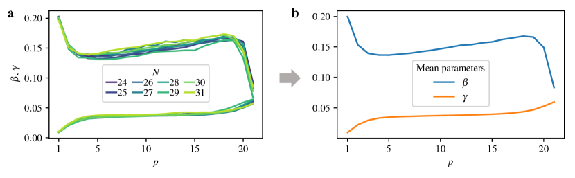
Figure 4: Visualization of how the fixed parameters are obtained. a, Optimized QAOA parameters $\bm{\beta}$ (top lines) and $\bm{\gamma}$ (bottom lines) for $p=21$. $\bm{\gamma}$ is multiplied by $N/24$ (constant factor of $\frac{1}{24}$ added for figure readability in both subfigures). b, Fixed parameters obtained by taking the arithmetic mean over the optimized parameters.

Theorem 1.

Suppose a constant-depth QAOA circuit $U_{\text{QAOA}}$ prepares a state $|\psi\rangle=U_{\text{QAOA}}|0\rangle^{\otimes N}$ with $N\geq 3,$ such that we have $\lvert\langle x^{*}|\psi\rangle\rvert\geq 1/\sqrt{p_{\text{opt}}}$, where $|x^{*}\rangle$ encodes an optimal solution to the $N$-bit LABS problem in a computational basis state, and we assume that $p_{\text{opt}}\geq 1/N$. Then, running Algorithm 1 with parameters $M\geq 1/\sqrt{p_{\text{opt}}}$ and failure probability $\delta$, runs with a gate complexity of $O(\text{poly}(N)\log(1/\delta)M)$ and finds $x^{*}$ with probability at least $1-\delta$.

Proof.

See Supplementary Information. SOM ∎

Choice of QAOA parameters $\beta,\gamma$

Our strategy for setting the QAOA parameters $\bm{\beta}$, $\bm{\gamma}$ used in our experiments is twofold. First, we optimize QAOA parameters for small $N$ using the FOURIER reparameterization scheme of Ref. Zhou et al., 2020. Second, we use the optimized parameters for small $N$ to compute fixed QAOA parameters that are then used for larger $N$. To apply the fixed parameters to an instance with a given size $N$, we rescale the parameters $\bm{\gamma}$ by $N$. SOM We discuss the parameter optimization scheme and the parameter rescaling in the Supplementary Information. SOM We note that the results presented above can be improved if better parameter setting strategies are used.

The procedure for obtaining the set of fixed QAOA parameters is visualized in Fig. 4. Specifically, we optimize QAOA parameters for a set of small instances with sizes $\{N_{j}\}_{j=1}^{M}$ attainable in simulation and set the fixed parameters to be the mean over the optimized parameters:

$$\bm{\beta}^{\text{Fixed}} =\frac{1}{M}\sum_{j=1}^{M}\bm{\beta}^{*}_{N_{j}},$$ (7)

$$\bm{\gamma}^{\text{Fixed}} =\frac{1}{M}\sum_{j=1}^{M}N_{j}\bm{\gamma}^{*}_{N_{j}},$$ (8)

where $\bm{\beta}^{*}_{N_{j}}$, $\bm{\gamma}^{*}_{N_{j}}$ are the QAOA parameters optimized for the LABS instance of size $N_{j}$ and $M$ is the number of optimized instances. Then the parameters used in QAOA for size $N$ are given by $\bm{\beta}^{\text{Fixed}},\frac{\bm{\gamma}^{\text{Fixed}}}{N}$. We use $24\leq N_{j}\leq 31$ ($M=8$).

Error detection by symmetry verification

The error detection scheme relies on the symmetry of phase operator defined by Eq. 2. As it commutes with both $\otimes_{i}^{N}\textsc{z}_{i}$ and $\otimes_{i}^{N}\textsc{x}_{i}$ operators, one can measure the value of these operators and perform postselection on the measurement outcomes. That is, the state after the phase operator should have the same z and x parity as before it. In the presence of an odd number of bit flip or phase flip errors that occur during the implementation of phase operators, the resulting state will not be in the +1 eigenspace of the two syndrome operators.

Experimentally, we divide the whole phase operator into $m$ splits such that each split has approximately the same number of two-qubit gates, and we perform syndrome checks at the end of each split to detect errors. The syndrome operators are mapped to ancillary qubits via sequential controlled-x or controlled-z gates and Hadamard gates applied before and after the partial phase operator. Since the number of two-qubit gates for the phase operators is higher than the number of gates used for the mapping by 2–3 orders of magnitude, additional errors introduced by ancillae are negligible. Furthermore, the crosstalk error probability during mid-circuit measurements is on the order of $10^{-5}$, considerably lower than the typical two-qubit-gate infidelity of $2\times 10^{-3}$ for the trapped-ion systems we used. Moses et al. (2023) As a result, our error detection scheme leads to large improvements in QAOA performance on hardware at the cost of the number of repetitions growing exponentially with the number of checks. Gonzales et al. (2023) We note that the performance of the error detection scheme can be further improved by implementing parity checks using fault-tolerant constructions. Self et al. (2022)

Scaling of classical solvers

All scaling coefficients are obtained by fitting a least-squares linear regression on the logarithm of TTS. The confidence intervals on the scaling coefficients are obtained by using the Student’s $t$-distribution and are reported with $95\%$ confidence.

We use commercial state-of-the-art branch-and-bound solvers in numerical experiments. Figure 1b and Table 1 show results obtained using Gurobi, Gur although we obtain similar results for CPLEX IBM ILOG CPLEX (see the Supplementary Information). The use of commercial branch-and-bound solvers is motivated by the observation that their scaling closely matches that reported in Ref. Packebusch and Mertens, 2016. Specifically, we observe that for both solvers the time to produce a certificate of optimality (TTO) scales with an exponent within a $95\%$ confidence interval of the $1.73$ exponent reported in Ref. Packebusch and Mertens, 2016. We note that unlike the solver presented in Ref. Packebusch and Mertens, 2016, commercial solvers are not parallelizable and can take advantage of only one CPU with at most tens of cores. Since QAOA is a heuristic and does not guarantee optimality, we additionally run branch-and-bound solvers until a solution with an exactly optimal merit factor is found, at which point the execution is stopped. The resulting TTS scales more favorably: for Gurobi, the scaling is $1.615^{N}$, with a $95\%$ confidence interval of $(1.571,1.659)$. All the numbers reported correspond to the mean CPU time, with the mean taken over 100 random seeds for $N\leq 32$ and 10 random seeds for $N>32$. We present additional details of classical solver benchmarking in the Supplementary Information. SOM

Branch-and-bound algorithms are the best-known exact solvers for the LABS problem. In the regime where proving optimality is out of reach and the goal is simply to efficiently obtain sequences with high merit factors, heuristic algorithms are preferable. The best runtimes and runtime scaling reported in the literature Gallardo et al. (2009) are from an algorithm known as Memetic Tabu. Memetic Tabu is a memetic algorithm, that is, an evolutionary algorithm augmented by local search. Specifically, an evolutionary algorithm is used to find initializations for tabu search, a metaheuristic that augments local neighborhood search with a data structure (known as the tabu list) that filters possible local moves if the potential solutions have been recently visited or diversification rules are violated. Glover and Laguna (1997) In terms of the runtime required to find optimal solutions in the regime where exact solutions have been found using branch-and-bound methods, Packebusch and Mertens (2016) Memetic Tabu has been observed to outperform both non-evolutionary methods as well as memetic algorithms that use simpler neighborhood search schemes such as steepest descent. To verify the scaling of tabu search on the regime of interest for comparison with QAOA, we use the implementation of Memetic Tabu in Ref. Bošković et al., 2016. For each length, we average the runtime over 50 random seeds, obtaining the scaling of the time-to-solution of $1.35^{N}$ with a $95\%$ confidence interval of $(1.33,1.38)$. This scaling closely matches the one reported in Ref. Bošković et al., 2017. We also note that solvers based on self-avoiding random walks Bošković et al. (2016) have been shown to be competitive with or outperform Memetic Tabu when the task is to find skew-symmetric SOM sequences with the lowest autocorrelation. These solvers are specialized to search for skew-symmetric sequences and do not naturally extend to the unrestricted LABS problem.

High-performance simulation of QAOA

Our numerical results are enabled by a custom scalable high-performance algorithm-specific QAOA simulator. We briefly describe the simulator here; for additional details and benchmarks comparing the developed simulator with the state-of-the-art methods for simulating QAOA the reader is referred to Ref. Lykov et al., .

In this work, the main goal of the numerical simulation of QAOA is to evaluate the expectation of the cost Hamiltonian $\langle C\rangle_{\text{MF}}$ and the success probability $p^{\text{opt}}$. Since $p^{\text{opt}}$ is exponentially small, it has to be evaluated with high precision. While many techniques can be leveraged for exact simulation, we opt to directly simulate the full quantum state as it is propagated through the QAOA circuit. We note in particular that tensor network techniques do not provide a benefit in this case since the circuit we simulate is deep and fully connected (see Ref. Lykov et al., for detailed comparison).

First, we leverage the observation that the cost Hamiltonian and hence the phase-separation operator are diagonal. This allows us to precompute the cost function evaluated at every binary input and multiply the exponentiated costs elementwise with the statevector to simulate the application of the phase-separation operator. This operation can be easily parallelized since it is an elementwise operation local to each element in the statevector. The same precomputed vector of cost function values is used to compute $\langle C\rangle_{\text{MF}}$ by taking the inner product with the final QAOA state. The cost of precomputation is amortized over the large number of objective evaluations performed during parameter optimization and is thereby negligible.

Second, we note that the mixing operator consists of an application of a uniform x rotation applied on each qubit. Therefore, each rotation operation can be computed by multiplying a fixed $2\times 2$ unitary matrix with a $2\times 2^{n-1}$ matrix constructed from reshaping the statevector. This step is parallelized by grouping the pairs of indices on which the $2\times 2$ unitary is applied.

We perform the simulations on the Polaris supercomputer located in Argonne Leadership Computing Facility. We distribute the simulation to 256 Polaris nodes with four NVIDIA A100 GPUs on each node and one AMD EPYC CPU. The CPU is used to manage the communication and the assembly of final results. Each GPU hosts a chunk of the full statevector and a chunk of the integer cost operator vector. Application of the cost operator does not require any communication since it is local to each element. The grouping in the mixing operator depends on index $i$ of the operator $\textsc{x}_{i}$ analogous to the grouping in the fast Walsh–Hadamard transform. Fino and Algazi (1976) For $i\leq n-\log_{2}(1024)=29$ the pairing is local within each GPU. For $i>29$ we use CUDA-enabled MPI to distribute full chunks between nodes, which requires space to be reserved for two statevector chunks on each GPU.

Author contributions

R. Shaydulin devised the project. J. Larson, N. Kumar, and R. Shaydulin implemented QAOA parameter optimization and the parameter setting schemes. R. Shaydulin and Y. Sun implemented the single-node version of the QAOA simulator. D. Lykov implemented the distributed version of the QAOA simulator and executed the large-scale simulations on Polaris. R. Shaydulin analyzed the simulation results. D. Herman and S. Hu developed the circuit optimization pipeline. C. Li implemented and analyzed the error detection scheme. M. DeCross and D. Herman executed the experiments on trapped-ion hardware, and C. Li analyzed the results. S. Chakrabarti, D. Lykov and P. Minssen benchmarked classical solvers. S. Chakrabarti, D. Herman and R. Shaydulin analyzed the generalized quantum minimum-finding enhanced with QAOA. J. Dreiling, J.P. Gaebler, T.M. Gatterman, J.A. Gerber, K. Gilmore, D. Gresh, N. Hewitt, C.V. Horst, J. Johansen, M. Matheny, T. Mengle, M. Mills, S.A. Moses, B. Neyenhuis, and P. Siegfried built, optimized, and operated the trapped-ion hardware. M. Pistoia led the overall project. All authors contributed to technical discussions and the writing of the manuscript.

Data availability

The data presented in this paper can be found at https://doi.org/10.5281/zenodo.8190275.

Code availability

The code used to produce the results in this paper can be found at https://github.com/jpmorganchase/QOKit.

Disclaimer

This paper was prepared for informational purposes with contributions from the Global Technology Applied Research center of JPMorgan Chase & Co., Argonne National Laboratory and Quantinuum LLC. This paper is not a product of the Research Department of JPMorgan Chase & Co. or its affiliates. Neither JPMorgan Chase & Co. nor any of its affiliates makes any explicit or implied representation or warranty and none of them accept any liability in connection with this position paper, including, without limitation, with respect to the completeness, accuracy, or reliability of the information contained herein and the potential Legal, compliance, tax, or accounting effects thereof. This document is not intended as investment research or investment advice, or as a recommendation, offer, or solicitation for the purchase or sale of any security, financial instrument, financial product or service, or to be used in any way for evaluating the merits of participating in any transaction.

The submitted manuscript includes contributions from UChicago Argonne, LLC, Operator of Argonne National Laboratory (“Argonne”). Argonne, a U.S. Department of Energy Office of Science laboratory, is operated under Contract No. DE-AC02-06CH11357. The U.S. Government retains for itself, and others acting on its behalf, a paid-up nonexclusive, irrevocable worldwide license in said article to reproduce, prepare derivative works, distribute copies to the public, and perform publicly and display publicly, by or on behalf of the Government. The Department of Energy will provide public access to these results of federally sponsored research in accordance with the DOE Public Access Plan http://energy.gov/downloads/doe-public-access-plan.

References

- Christoph Dürr and Peter Høyer (1996) Christoph Dürr and Peter Høyer, arXiv:quant-ph/9607014 (1996).
- Chakrabarti et al. (2022) S. Chakrabarti, P. Minssen, R. Yalovetzky, and M. Pistoia, arXiv:2210.03210 (2022).
- Somma et al. (2008) R. D. Somma, S. Boixo, H. Barnum, and E. Knill, Physical Review Letters 101 (2008).
- Wocjan and Abeyesinghe (2008) P. Wocjan and A. Abeyesinghe, Physical Review A 78 (2008).
- Hastings (2018) M. B. Hastings, Quantum 2, 78 (2018).
- Dalzell et al. (2023) A. M. Dalzell, N. Pancotti, E. T. Campbell, and F. G. Brandão, in Proceedings of the ACM Symposium on Theory of Computing (2023).
- Hogg and Portnov (2000) T. Hogg and D. Portnov, Information Sciences 128, 181 (2000).
- Farhi et al. (2014) E. Farhi, J. Goldstone, and S. Gutmann, arXiv:1411.4028 (2014).
- Zhou et al. (2020) L. Zhou, S.-T. Wang, S. Choi, H. Pichler, and M. D. Lukin, Physical Review X 10, 021067 (2020).
- Basso et al. (2022) J. Basso, E. Farhi, K. Marwaha, B. Villalonga, and L. Zhou, Proceedings of the Conference on the Theory of Quantum Computation, Communication and Cryptography 7, 1 (2022).
- Boulebnane and Montanaro (2022) S. Boulebnane and A. Montanaro, arXiv:2208.06909 (2022).
- Sureshbabu et al. (2023) S. H. Sureshbabu, D. Herman, R. Shaydulin, J. Basso, S. Chakrabarti, Y. Sun, and M. Pistoia, arXiv:2305.15201 (2023).
- Boehmer (1967) A. Boehmer, IEEE Transactions on Information Theory 13, 156 (1967).
- Schroeder (1970) M. Schroeder, IEEE Transactions on Information Theory 16, 85 (1970).
- Bernasconi (1987) J. Bernasconi, Journal de Physique 48, 559 (1987).
- Mertens and Bessenrodt (1998) S. Mertens and C. Bessenrodt, Journal of Physics A: Mathematical and General 31, 3731 (1998).
- Golay (1977) M. Golay, IEEE Transactions on Information Theory 23, 43 (1977).
- Bošković et al. (2016) B. Bošković, F. Brglez, and J. Brest, “A GitHub Archive for Solvers and Solutions of the LABS problem,” (2016).
- Packebusch and Mertens (2016) T. Packebusch and S. Mertens, Journal of Physics A: Mathematical and Theoretical 49, 165001 (2016).
- (20) D. Lykov, R. Shaydulin, Y. Sun, Y. Alexeev, and M. Pistoia, “Fast simulation of high-depth QAOA,” In preparation.
- Gallardo et al. (2009) J. E. Gallardo, C. Cotta, and A. J. Fernández, Applied Soft Computing 9, 1252 (2009).
- Lemieux et al. (2020) J. Lemieux, B. Heim, D. Poulin, K. Svore, and M. Troyer, Quantum 4, 287 (2020).
- Boixo et al. (2015) S. Boixo, G. Ortiz, and R. Somma, The European Physical Journal Special Topics 224, 35 (2015).
- Pino et al. (2021) J. M. Pino, J. M. Dreiling, C. Figgatt, J. P. Gaebler, S. A. Moses, M. S. Allman, C. H. Baldwin, M. Foss-Feig, D. Hayes, K. Mayer, C. Ryan-Anderson, and B. Neyenhuis, Nature 592, 209 (2021).
- Moses et al. (2023) S. A. Moses et al., arXiv:2305.03828 (2023).
- Gonzales et al. (2023) A. Gonzales, R. Shaydulin, Z. H. Saleem, and M. Suchara, Scientific Reports 13 (2023).
- Debroy and Brown (2020) D. M. Debroy and K. R. Brown, Physical Review A 102 (2020).
- Bošković et al. (2017) B. Bošković, F. Brglez, and J. Brest, Applied Soft Computing 56, 262 (2017).
- (29) Supplementary Information: Evidence of Scaling Advantage for the Quantum Approximate Optimization Algorithm on a Classically Intractable Problem.
- Sanders et al. (2020) Y. R. Sanders, D. W. Berry, P. C. Costa, L. W. Tessler, N. Wiebe, C. Gidney, H. Neven, and R. Babbush, PRX Quantum 1 (2020).
- van Apeldoorn et al. (2020) J. van Apeldoorn, A. Gilyén, S. Gribling, and R. de Wolf, Quantum 4, 230 (2020).
- Boyer et al. (1998) M. Boyer, G. Brassard, P. Høyer, and A. Tapp, Fortschritte der Physik 46, 493 (1998).
- Shaydulin and Pistoia (2023) R. Shaydulin and M. Pistoia, arXiv:2303.02064 (2023).
- He et al. (2023) Z. He, R. Shaydulin, S. Chakrabarti, D. Herman, C. Li, Y. Sun, and M. Pistoia, arXiv:2305.03857 (2023).
- Pelofske et al. (2023a) E. Pelofske, A. Bärtschi, J. Golden, and S. Eidenbenz, arXiv:2306.03238 (2023a).
- Pelofske et al. (2023b) E. Pelofske, A. Bärtschi, and S. Eidenbenz, in Lecture Notes in Computer Science (Springer Nature Switzerland, 2023) pp. 240–258.
- Niroula et al. (2022) P. Niroula, R. Shaydulin, R. Yalovetzky, P. Minssen, D. Herman, S. Hu, and M. Pistoia, Scientific Reports 12 (2022).
- Shaydulin and Galda (2021) R. Shaydulin and A. Galda, in IEEE International Conference on Quantum Computing and Engineering (2021).
- Kakkar et al. (2022) A. Kakkar, J. Larson, A. Galda, and R. Shaydulin, in IEEE International Conference on Quantum Computing and Engineering (2022).
- Babbush et al. (2021) R. Babbush, J. R. McClean, M. Newman, C. Gidney, S. Boixo, and H. Neven, PRX Quantum 2 (2021).
- Brassard et al. (2002) G. Brassard, P. Høyer, M. Mosca, and A. Tapp, Contemporary Mathematics , 53 (2002).
- Self et al. (2022) C. N. Self, M. Benedetti, and D. Amaro, arXiv:2211.06703 (2022).
- (43) Gurobi Optimization, www.gurobi.com.
- (44) IBM ILOG CPLEX, International Business Machines Corporation .
- Glover and Laguna (1997) F. Glover and M. Laguna, Tabu Search (Kluwer Academic Publishers, Norwell, MA, USA, 1997).
- Fino and Algazi (1976) Fino and Algazi, IEEE Transactions on Computers C-25, 1142 (1976).