Generative Image Priors for MRI Reconstruction Trained from Magnitude-Only Images

Abstract

1 Purpose

In this work, we present a workflow to construct generic and robust generative image priors from magnitude-only images. The priors can then be used for regularization in reconstruction to improve image quality.

2 Methods

The workflow begins with the preparation of training datasets from magnitude-only MR images. This dataset is then augmented with phase information and used to train generative priors of complex images. Finally, trained priors are evaluated using both linear and nonlinear reconstruction for compressed sensing parallel imaging with various undersampling schemes.

3 Results

The results of our experiments demonstrate that priors trained on complex images outperform priors trained only on magnitude images. Additionally, a prior trained on a larger dataset exhibits higher robustness. Finally, we show that the generative priors are superior to $\ell^{1}$-wavelet regularization for compressed sensing parallel imaging with high undersampling.

4 Conclusion

These findings stress the importance of incorporating phase information and leveraging large datasets to raise the performance and reliability of the generative priors for MRI reconstruction. Phase augmentation makes it possible to use existing image databases for training.

5 Introduction

Regularizing the inverse problem for parallel MRI reconstruction is an effective and flexible approach for improving image quality, especially when the obtained k-space is highly undersampled in order to shorten the scan time. The prior knowledge that images are sparse in a transform domain as used in compressed sensing is known as $\ell^{1}$-norm regularization^{1, 2}. Combined with incoherent sampling, this allows recovery of images from moderately undersampled k-space data with clinically acceptable quality^{3, 4}.

The application of deep learning makes it possible to further increase undersampling without compromising image quality by leveraging the learned prior information from a training dataset. Popular methods can be classified into three main categories: supervised methods^{5, 6}, where the neural network is a result of unrolling an iterative algorithm trained with labels and used to predict the reconstruction, self-supervised methods^{7, 8} that involve splitting the acquired k-space data of a scan into two disjoint sets where only the first set is used for reconstruction and the second set provides supervision, and decoupled methods^{9, 10, 11}, where a generative model or a denoiser is trained to learn the empirical distribution of data which is then used in a conventional iterative reconstruction method. In the following, we will refer to a generative model also as a prior.

Training in supervised methods based on unrolled iterative algorithms requires not only fully sampled k-space data, but also pre-defined sampling patterns and precomputed coil sensitivities. The prior knowledge learned in this way then pertains to these pre-defined settings. However, protocol settings for clinical and research are changed often, and the preparation of reference data, which is used as labels for training, is costly. Decoupled methods are able to avoid these constraints, and the learned prior can even be transferred to new scenarios such as different contrasts¹².

As a crucial part of decoupled methods, the use of generative models, such as variational autoencoders and autoregressive models, was investigated previously by formulating the linear reconstruction problem for accelerated MRI from the Bayesian perspective and solving it via maximum a posterior (MAP) estimation ^{9, 11}. More recently, diffusion models emerged as effective priors for MRI reconstruction and were combined with Monte Carlo methods that sampling the posterior^{13, 14, 12}. However, their performance is heavily dependent on the size and quality of the training dataset and the computational resources available.

For this reason, it is desirable to use existing databases of MR images for training. But as shown here, training from magnitude-only images leads to inferior priors. This work therefore proposes a new approach to construct priors using magnitude-only training images as illustrated in Figure 1. The workflow begins with the preparation of training datasets from magnitude-only MR images. This dataset is then augmented with phase information and used to train generative priors on complex images. Finally, trained priors can be used with both linear and nonlinear reconstruction for compressed sensing parallel imaging. The contributions of our work are:

1. We demonstrate that priors trained on complex images are superior to priors trained only on magnitude images.

2. We leverage a diffusion model trained on a small dataset (~1000 images) of complex images to augment a much larger dataset (~80k images) for which the phase information of the image is not available.

3. We show that we can train more robust generative priors by incorporating knowledge from a larger training dataset, which contains a diverse range of images. Such a database can be obtained by phase augmentation of magnitude images which are readily available.

4. By integrating the priors as regularization terms into existing reconstruction techniques, we maintain the flexibility of existing reconstruction algorithms that can be used with various undersampling schemes and receive coils.

Parts of this work have been presented in Refs. Luo__2022a, Luo__2021.

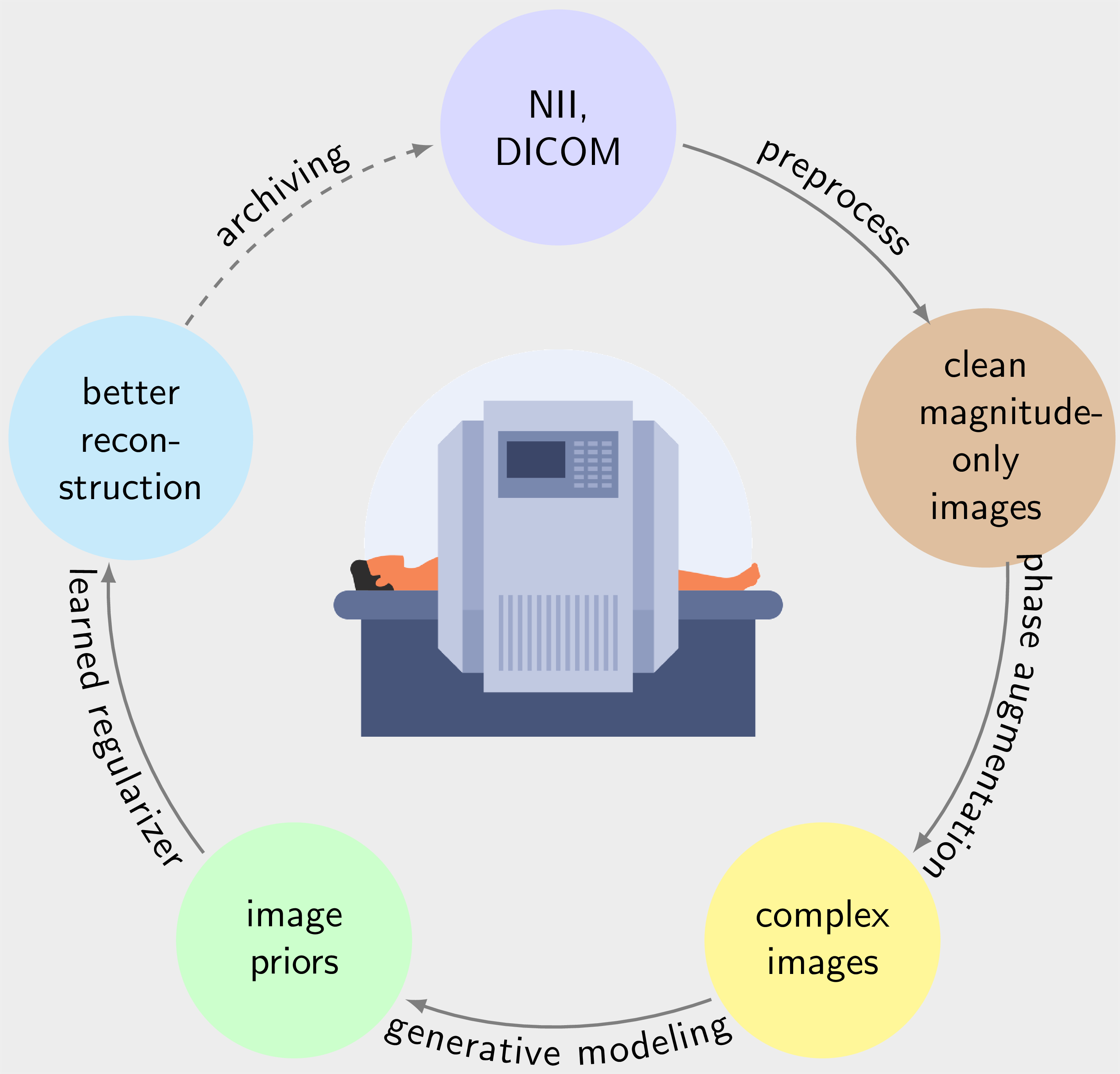
Figure 1: The proposed workflow for extracting prior knowledge and using it for regularization in image reconstruction. It comprises data preparation, phase augmentation, generative modeling, and concludes with the use as learned regularizers in reconstruction.

6 Theory

6.1 Linear and nonlinear reconstruction

The reconstruction in parallel imaging can be formulated as an inverse problem

$$F(\mathbf{x},\mathbf{c})\coloneqq(\mathcal{F}_{S}(\mathbf{x}\odot c_{1}),\cdots,\mathcal{F}_{S}(\mathbf{x}\odot c_{N}))=\mathbf{y}~{},$$ (1)

where $\mathcal{F}_{S}$ is an undersampled multi-channel Fourier transform operator and the correspondingly obtained k-space data is $\mathbf{y}=(y_{1},\cdots,y_{nc})^{T}$; $\mathbf{y}\in\mathbb{C}^{d\times nc}$, $\mathbf{x}\in\mathbb{C}^{n\times n}$ denotes the image content and $\mathbf{c}=(c_{1},\cdots,c_{nc})^{T}$; $\mathbf{c}\in\mathbb{C}^{n\times n\times nc}$ denotes the coil sensitivities. Equation 1 can be solved in the following two ways.

One common way for MR image reconstruction is to predetermine the coil sensitivities $\mathbf{c}$ from a reference scan or from a fully sampled k-space center. Following coil estimation, we can solve the linear inverse problem using by optimization regularized least-squares functional

$$\underset{\mathbf{x}}{\min}\frac{1}{2}\|F_{\mathbf{c}}(\mathbf{x})-\mathbf{y}\|^{2}+\alpha R(\mathbf{x}),$$ (2)

where $F_{\mathbf{c}}(\mathbf{x}):=F(\mathbf{x},\mathbf{c})$ is a linear operator and $R(\mathbf{x})$ is the regularization term employing prior knowledge about the image, such as $\ell^{2}$ regularization¹⁷, total variation², $\ell^{1}$-sparsity¹, or a learned log-likelihood function¹¹.

Alternatively, both image and coil sensitivities can be jointly estimated from the same acquired data^{18, 19}. Ref. Uecker_Magn.Reson.Med._2008 formulates MR image reconstruction as a nonlinear inverse problem and proposes to solve Equation Equation 1 using the Iteratively Regularized Gauss Newton Method (IRGNM). This method linearizes the nonlinear inverse problem at each Gauss Newton step $k$, and estimates the update $\delta\mathbf{m}\coloneqq(\delta\mathbf{x},\delta\mathbf{c})$ for the pair $\mathbf{m}^{k}\coloneqq(\mathbf{x}^{k},\mathbf{c}^{k})$ by minimizing a regularized least-squares functional for the linearized sub-problem

$$\underset{\delta\mathbf{m}}{\min} \frac{1}{2}\|F^{\prime}(\mathbf{m}^{k})\delta\mathbf{m}~{}+~{}F(\mathbf{m}^{k})~{}-~{}\mathbf{y}\|^{2}$$

$$~{}+~{}\beta^{k}\mathcal{W}(\mathbf{c}^{k}~{}+~{}\delta\mathbf{c})~{}+~{}\alpha^{k}{R}(\mathbf{x}^{k}~{}+~{}\delta\mathbf{x})~{}.$$ (3)

Here, $\mathcal{W}(\mathbf{c})=\|w\odot\mathcal{F}\mathbf{c}\|^{2}$ is a penalty on the high Fourier coefficients of the coil sensitivities and $R(\mathbf{x})$ is a regularization term on the image $\mathbf{x}$, e.g., $\ell_{2}$-norm¹⁹, $\ell_{1}$-sparsity in the wavelet domain²⁰, or total variation²¹. The $\alpha_{k}$ and $\beta_{k}$ are decreasing in each iteration step.

6.2 Learned priors as regularization

Learned prior knowledge can be used for regularization in image reconstruction. Generative priors, such as variational autoencoder, autoregressive models (e.g., PixelCNN), and diffusion models, are used to incorporate empirical knowledge about images into iterative optimization algorithms. We want to use generative priors directly as a drop-in replacement for conventional priors in existing image reconstruction algorithms, which are often based on proximal methods.

The proximal operator for the log-prior $\log p(\mathbf{x})$ is defined as

$$\operatorname{prox}_{t}(\mathbf{z})~{}=~{}\underset{\mathbf{x}}{\arg\min}~{}\frac{1}{2t}\|\mathbf{x}-\mathbf{z}\|^{2}+\log p(\mathbf{x})~{}.$$ (4)

When the mapping above is not analytically computable, the proximal operator could be approximated by minimizing Equation 4 using gradient descent. Note that the minimization problem for the proximal operator is the same as for a denoising problem for complex Gaussian noise²². Assuming some regularity of the prior and noise-like properties of the error during reconstruction, the gradient can be expected to always point in the same directions towards denoised images. Therefore, the optimality condition at the solution is approximately

$$0\approx\frac{1}{t}(prox_{t}(\mathbf{z})-\mathbf{z})+\nabla_{\mathbf{x}}\log p(\mathbf{x})~{}.$$

The solution is then equivalent to a single gradient-descent step with an arbitrary initial guess and unit step size

$$\operatorname{prox}_{t}(\mathbf{z}) \approx\mathbf{z}-t\nabla_{\mathbf{x}}\log p(\mathbf{x})~{},$$

which simply yields a gradient-descent step for the log-prior in the overall algorithm. In this work, two types of log-priors are used which are described below.

1. This prior is formulated using a joint distribution over the elements of an image vector

   $$\log p(\mathbf{x};\mathrm{NET}(\hat{\Theta},\mathbf{x}))=\log p(x^{(1)})\prod_{i=2}^{n^{2}}p(x^{(i)}\mid x^{(1)},..,x^{(i-1)})~{},$$ (5)

   where the neural network $\mathrm{NET}(\hat{\Theta},\mathbf{x})$ predicts the distribution parameters of a mixture of logistic distributions that is used to describe every pixel and where the dependencies between the channels for the real and imaginary parts are described with nonlinear dependencies¹¹. All these parameters used to probabilistically model the image are predicted by a causal network²³ that encodes the relationship between pixels as formulated in Equation 5. The gradient of $\log p(\mathbf{x};\mathrm{NET}(\hat{\Theta},\mathbf{x}))$ with respect to $\mathbf{x}$ can be computed by back-propagation through the neural network.

2. The diffusion probabilistic model proposed in Ref. Sohldickstein_ICML_2015 is constructed with a forward Markovian process and a learned reverse process. The forward process is to gradually transfer a data distribution $q(\mathbf{x}_{0})$ to a smoother known distribution $q(\mathbf{x}_{N})$, e.g., a Gaussian distribution, by adding noise to data points. The reverse process is to undo this forward process with learned reverse transitions, which are described as

   $$p_{\theta}(\mathbf{x}_{i-1}\mid\mathbf{x}_{i}) =\mathcal{CN}(\mathbf{x}_{i-1}\mid\mu_{\theta}(\mathbf{x}_{i},i),\tau_{i}^{2}\mathbf{I})\,,$$ (6)

   where $\tau_{i}$ can be computed from the noise scales $\sigma_{i}$ at each step and $\mu_{\theta}(\mathbf{x}_{i},i)$ can be understood as a denoised image based on the smoothed prior at each noise level. Instead of learning this distribution directly, the gradient of the log-prior is learned for all noise scales

   $$\nabla_{\mathbf{x}_{i}}\log p_{\boldsymbol{\theta}}\left(\mathbf{x}_{i-1}\mid\mathbf{x}_{i}\right) =\frac{1}{\tau_{i}^{2}}\left(\sigma_{i}^{2}-\sigma_{i-1}^{2}\right)\mathbf{s}_{\boldsymbol{\theta}}\left(\mathbf{x}_{i-1},i\right)~{},$$

   where $\mathbf{s}_{\theta}(\mathbf{x}_{i},i)$ is a trained score network²⁵, which is computationally efficient because it avoids backpropagation. We refer the reader to Ref. Luo_Magn.Reson.Med._2023 for details about this method. The reverse transitions start with $\sigma_{max}$ and end at a $\sigma_{min}\approx 0$. In this work we use $\sigma_{max}=0.3$ and $\sigma_{min}=0.01$, and

   $$\sigma_{i}=\sigma_{min}+\sigma_{max}\cdot\log(1+(1-i/N)\cdot(\mathsf{e}-1))~{}.$$

   Here, $\mathsf{e}$ is Euler constant and $N$ is the number of noise scales which in this work also corresponds to the total number of iterations of the reconstruction algorithm.

For linear reconstruction, the two regularization terms can be directly plugged into proximal optimization algorithms available in image reconstruction frameworks, such as the Fast Iterative Soft-Thresholding Method (FISTA)²⁶, or the Alternating Direction Methods of Multipliers (ADMM)²⁷.

Similarly, for nonlinear inverse problems, we can apply the regularization terms to the linearized sub-problem in Equation 3. In nonlinear reconstruction, the image content $\mathbf{x}$ is usually smooth at early Gauss Newton steps and the distribution of $\mathbf{x}$ is far from the learned empirical distribution. Correspondingly, in this work, the Gauss Newton optimization is split into two stages. In the first stage, an $\ell_{2}$-norm regularization is applied, and the method of conjugate gradients (CG) is used to minimize Equation 3. In the second stage, i.e., the later Gauss-Newton steps, FISTA is utilized with the proximal operators. The entire algorithm is outlined in Algorithm 1.

Algorithm 1 Two-stage IRGNM for NLINV reconstruction

1:Inputs:

2:      y - kspace data, n - MaxIter, r - RegIter

3:Initialization:

4:      $\mathbf{x}^{0}=\mathbf{1},~{}\mathbf{c}^{0}=\mathbf{0},~{}\alpha^{0}=1,~{}\beta^{0}=1$

5:for $k~{}\mathrm{in}~{}\{0,\>\dots,\>\mathrm{n-1}\}$ do

6:     if  $k<\mathrm{n-r}$ then

7:         $R(\mathbf{x})~{}=~{}\|\mathbf{x}\|^{2}$

8:         Estimate $\delta\mathbf{x},~{}\delta\mathbf{c}$ in Equation 3 with CG

9:     else

10:         $R(\mathbf{x})~{}=~{}\mathrm{log~{}p}(\mathbf{x})$  or  $\|\Psi\mathbf{x}\|^{1}$

11:         Estimate $\delta\mathbf{x},~{}\delta\mathbf{c}$ in Equation 3 with FISTA

12:     end if

13:     $\mathbf{x}^{k+1}=\mathbf{x}^{k}+\delta\mathbf{x},\>\mathbf{c}^{k+1}=\mathbf{c}^{k}+\delta\mathbf{c}$

14:     $\alpha^{k+1}=\max(\alpha_{\min},\>\alpha^{k}/2)$

15:     $\beta^{k+1}=\beta^{k}/2$

16:end for

7 Methods

In this section, we first describe how we implemented the proposed workflow, as shown in Figure 1, for extracting prior knowledge from an image dataset and then how we use the learned prior for regularization in image reconstruction. We detail how we evaluated the performance of the priors used for image regularization in different settings.

7.1 Preprocessing of the training dataset

As for training data, we use human brain images from the Autism Brain Imaging Data Exchange (ABIDE)^{28, 29}. After we downloaded the dataset, which comes in 3D volumes in NII format, we performed the following steps to preprocess it.

1. Load each 3D volume and resample it with the conform function of NiBabel³⁰ to make its axial plane have a size of 256 $\times$ 256.

2. Split the volume into 2D image slices that are oriented in axial plane.

3. Add background Gaussian noise ($\mu=0.003,\sigma=5$) to all slices, and then normalize every slice by dividing by its maximum pixel value.

4. Crop a 30 $\times$ 30 patch from the XY-corner of each normalized slice and compute the mean $\mu$ and standard deviation $\sigma$ over all pixels of the patch.

5. Exclude slices from phase augmentation when mean $\mu<0.04$ and standard deviation $\sigma<0.0061$.

7.2 Phase augmentation

ABIDE images are provided solely as magnitude images without phase information. The magnitude of an MR image is determined by the proton density, relaxation effects, and receive fields, while the phase is affected by the phase of the receive field, inhomogeneities of the static field, eddy currents, and chemical shift. Phase augmentation can be used to add a phase to obtain more realistic complex-valued images. Here, we describe a procedure to obtain new samples with phase information from magnitude images using a prior previously trained prior for complex-valued images. The method is based on previous research²⁴ for the sampling of a posterior. Given the likelihood term of the magnitude $p(\mathbf{m}|\mathbf{x})$ and a prior for complex-valued images $p(\mathbf{x})$, the posterior of the complex image is proportional to $p(\mathbf{x}|\mathbf{m})\propto p(\mathbf{x})\cdot p(\mathbf{m}|\mathbf{x})$ where

$$\bar{\mathbf{m}}=\sqrt{\mathbf{x}_{r}^{2}+\mathbf{x}_{i}^{2}}\ ,$$

and $\mathbf{x}_{r}$ and $\mathbf{x}_{i}$ are the real part and imaginary part, respectively. The likelihood term for a given magnitude image $\mathbf{m}$ is $p(\mathbf{m}|\mathbf{x})=\delta(\mathbf{m}-\sqrt{\mathbf{x}_{r}^{2}+\mathbf{x}_{i}^{2}})$. To be able to apply gradient-based methods, we approximate this with a narrow Gaussian distribution

$$p(\mathbf{m}|\mathbf{x})\propto\exp\bigl{(}-\epsilon\bigl{\|}\mathbf{m}-\sqrt{\mathbf{x}_{r}^{2}+\mathbf{x}_{i}^{2}}\bigr{\|}_{2}^{2}\bigr{)}.$$

Specifically, we initialize samples with random complex Gaussian noise and then transfer them gradually to the distribution of complex images with learned transition kernels ${p}_{\theta}(\mathbf{x}_{n}|\mathbf{x}_{n+1})$. We run unadjusted Langevin iterations sequentially at each intermediate distribution

$$\mathbf{x}_{n}^{k+1}\leftarrow\mathbf{x}_{n}^{k}+\frac{\gamma}{2}\nabla_{\mathbf{x}}\log{p}_{\theta}(\mathbf{x}_{n}^{k}\mid\mathbf{x}_{n+1}^{\mathrm{K}})+\frac{\gamma}{2}\nabla_{\mathbf{x}}\log p(\mathbf{m}|\mathbf{x}_{n}^{k})+\sqrt{\gamma}\mathbf{z}~{}.$$

Here, $\mathbf{z}$ is complex Gaussian noise, which introduces random fluctuations and $\gamma$ controls the step size of the Langevin algorithm. The sampling algorithm was implemented with TensorFlow and used with the pre-trained generative model $\mathrm{NET}_{1}$ from Ref. Luo_Magn.Reson.Med._2023, which was trained on the small dataset from Ref. Luo_Magn.Reson.Med._2020. For each magnitude image five complex images were generated.

7.3 Training of priors

Table 1: Datasets and computational resources used to train the fix different priors used in this work.

Prior		Model	Phase	Nr. of Images	MR Contrasts	GPUs	Parameters	Time $\times$ epochs
PSC	(small, complex)	PixelCNN	preserved	1000	T1, T2, T2-FLAIR, T${}^{*}_{\mathrm{2}}$	4$\times$A100, 80G	~22M	~40s $\times$ 500
PSM	(small, magnitude)	PixelCNN	not available	1000	T1, T2, T2-FLAIR, T${}^{*}_{\mathrm{2}}$	4$\times$V100, 32G	~22M	~144s $\times$ 500
PLM	(large, magnitude)	PixelCNN	not available	23078	MPRAGE	4$\times$A100, 80G	~22M	~748s $\times$ 100
PLC	(large, complex)	PixelCNN	generated	23078	MPRAGE	3$\times$A100, 80G	~22M	~1058s $\times$ 100
DSC	(SMLD, complex)	Diffusion	generated	79058	MPRAGE	4$\times$A100, 80G	~8M	~2330s $\times$ 50
DPC	(DDPM, complex)	Diffusion	generated	79058	MPRAGE	8$\times$V100, 32G	~8M	~1430s $\times$ 200

In total, we trained six priors in this work. The PixelCNN priors, P_SC and P_SM, were trained on the small brain image dataset used in Ref. Luo_Magn.Reson.Med._2020 using complex and magnitude images, respectively. P_LM and P_LC were trained on a subset of the preprocessed ABIDE dataset corresponding of 500 volumes and the corresponding phase-augmented complex images, respectively. We also trained two diffusion priors, SMLD (D_SC) and DDPM (D_PC) with phase-augmented images using the full ABIDE dataset with 1206 volumes.

During the training, images were normalized to have a maximum magnitude of one and then subjected to random mirroring, flipping, and rotation prior to being fed into the neural network. Complex images were fed as two-channel maps (i.e., real and imaginary), and magnitude images were fed as single-channel maps. The networks used for PixelCNN and the diffusion models were implemented with TensorFlow (TF) and the optimizer ADAM was used for all training tasks, which was performed using multi-GPU systems using different GPUs (Nvidia Corporation, Santa Clara, CA, USA).

1. We trained this generative model by maximizing the probability of the joint distribution over all the pixels in the image using the discretized logistic mixture distribution loss proposed in Ref. Salimans_ICLR_2017.

2. There exist two types of diffusion models that are based on the denoising score matching method³¹, namely, denoising Score Matching with Langevin Dynamics (SMLD)³² and Denoising Diffusion Probabilistic Models (DDPM)³³. Both are unified in a common framework described in Ref. Song_ICLR_2021. We train diffusion priors using both SMLB and DDPM with the same Refine-Net³⁴ architecture also used in Ref. Luo_Magn.Reson.Med._2023. The loss function used to train the score network $\mathbf{s}_{\theta}(\mathbf{x}_{i},i)$ is given by

   $$\theta^{\ast}=\underset{\theta}{\arg\operatorname*{min}}~{}\sum_{i}\mathbb{E}_{\mathbf{x}_{0}}\mathbb{E}_{\mathbf{x}_{i}|\mathbf{x}_{0}}\bigl{[}\lambda_{i}\bigl{\|}\mathbf{s}_{\theta}(\mathbf{x}_{i},i)-\nabla_{\mathbf{x}_{i}}\log p\left(\mathbf{x}_{i}\mid\mathbf{x}_{0}\right)\bigr{\|}_{2}^{2}\bigr{]}\,$$

   where $\lambda_{i}$ is the weighting function described in Ref. Song_ICLR_2021.

Information about priors and training is detailed in Table 1.

7.4 Experimental evaluation

In this section, we use Berkeley Advanced Reconstruction Toolbox (BART)³⁵ to evaluate the trained priors using Parallel Imaging Compressed Sensing (PICS) and Nonlinear Inversion (NLINV). The corresponding commands have an option for loading an exported TensorFlow computation graph and using it for regularization. The exported graph was wrapped into a nonlinear operator and then used in the proximal mapping step³⁶. For the linear reconstruction using PICS, the coil sensitivities are estimated with ESPIRiT³⁷. In the nonlinear reconstruction using NLINV, Algorithm 1 was implemented with the nonlinear operator framework³⁶.

We then performed different experiments using PICS and NLINV for the six priors using different sampling patterns in comparison to zero-filled, $\ell_{2}$, $\ell_{1}$-wavelet reconstructions and coil-combined images form fully sampled data. Here, we used a T₁-weighted k-space from the test dataset used in Ref. Luo_Magn.Reson.Med._2020. We additionally performed a study using quantitative image quality metrics using 3D MPRAGE data to evaluate the impact of the size of the training dataset, and performed an evaluation study with human readers for six fully sampled 3D TurboFLASH datasets as described below.

1. We performed retrospective reconstruction using all six priors. Three types of undersampling pattern were used in this retrospective experiment, including five-fold acceleration along phase direction, two-times and three times acceleration along frequency and phase direction, respectively, and 8.2-times undersampling using Poisson-disc sampling. While the acceleration along frequency-encoding direction is not realistic, we use it to explore how the priors handle different 2D different patterns. In a later experiment below, we then use 3D k-space acquisitions where these sampling pattern are feasible.

2. We performed the reconstruction using P_SC and P_LC. The k-space data were acquired from the brain of a healthy volunteer using MPRAGE sequence on 3T Siemens Skyra scanner (Siemens Healthineers, Erlangen, Germany) with 16-channel head coils. The protocol parameters were: TE = 2.45 ms, flip angle $\alpha=8$°, TI = 900 ms, and TR = 2000 ms, 4/5 partial parallel Fourier imaging, and 2-fold acceleration along one phase encoding direction. This acquired 3D volume has dimensions 256 $\times$ 256 $\times$ 224 and isotropic voxel size of 1 mm. We further undersampled the acquired 3D k-space data two and three times along two phase-encoding directions with the central region of size 30 $\times$ 25 reserved. The reconstruction was performed slice-by-slice in a 2D plane. To quantitatively assess the robustness of the priors, we computed PSNR and SSIM for the P_LC-regularized reconstruction from 4 and 6-times undersampled k-space against the P_LC-regularized reconstruction from 2-times undersampled k-space and compared it to PSNR and SSIM for the $\ell_{2}$-wavelet regularization and the prior P_SC.

3. For reconstruction of 3D data sets, we chose the two diffusion models (D_SC and D_PC) that are less computationally expensive than PixelCNN. The k-space data was acquired from 6 volunteers using a 3D TurboFLASH sequence (TE = 3.3 ms, TR = 2250 ms, TI = 900 ms, flip angle $\alpha=9$°) using a 3T Siemens Prisma scanner and a 64-channel head-coil. These acquired 3D volumes have dimensions 256 $\times$ 256 $\times$ 176 and isotropic size of 1 mm. We undersampled the acquired 3D k-space data using a prospectively feasible Poisson-disc pattern with 8.2-time undersampling. When applying the prior during reconstruction, all slices in the axial plane are padded to a size of 256 $\times$ 256 Following this, the prior is applied on all slices in parallel and the computed gradient will be resized to the original image size. The reconstructed volumes were blindly evaluated by three clinicians with variable experience in neuroimaging (~20 years, ~10 years, ~5 years). $\ell_{1}$-wavelet reconstructions and a reference reconstructed from fully sampled k-space data by coil-combination were included in this evaluation study. The grading scale used in this study ranged from 5 to 1, where a score of 5 represents "excellent" image quality and a 1 denotes "bad" image quality.

8 Results

Figure 2(a) shows three magnitude images of different quality from the ABIDE dataset and the corresponding magnitude and phase maps of complex-valued images generated by phase augmentation. The magnitude part of the generated images stays very close to the original image but exhibits a bit less noise. The phase of the generated images maps is smooth and looks realistic with some random variations as expected.

In Figure 2(b), we present the magnitude and phase from images reconstructed using PICS with ESPIRiT sensitivities and NLINV using the same P_SC prior for 8.2-times undersampled Poisson-disc k-space data in comparison to a zero-filled image and fully-sampled reference. For both methods, similar reconstructions with excellent quality can be obtained for this prior for linear and non-linear reconstruction. This prior trained from a small dataset of complex-valued images will serve as a baseline for the other learned priors.

(a)
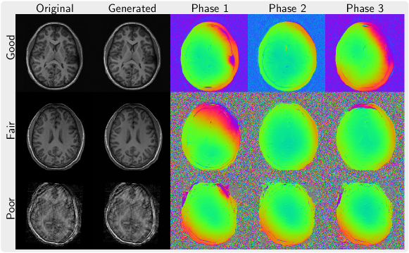
(b)

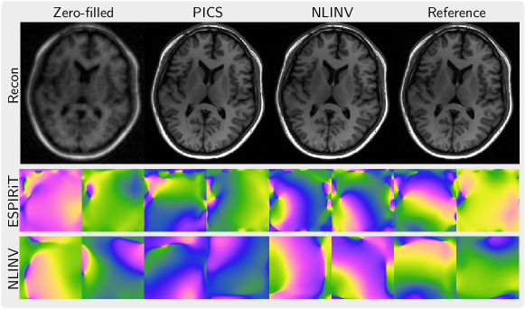
Figure 2: (a) Human brain images of different quality are shown (rows). On the left, the original magnitude-only images are compared to the magnitude of a corresponding image generated using phase augmentation. On the right, the phase maps of three different generated images are shown. (b) Linear (PICS) and nonlinear (NLINV) reconstruction using a prior for complex-valued images trained from a dataset of images with preserved phase P_SC in comparison to zero-filled image and a fully-sampled reference. The magnitude and coil sensitivity maps estimated with ESPIRiT and NLINV are shown below.

8.1 The influence of phase maps

Figure 3 presents the magnitude and phase of images that are reconstructed using PICS with priors trained from magnitude image, complex images with preserved phase, and complex images with generated using our phase augmentation method While the priors P_SM and P_LM trained from magnitude images can remove folding artifacts introduced by undersampling, they exhibit over-smoothing of the magnitude as indicated by its lower PSNR and SSIM values and also demonstrates poor capabilities in denoising the phase. In contrast, the prior P_SC trained on complex-valued images performs much better. Furthermore, the priors P_LC and D_SC trained on phase-augmented images and perform almost as well. Very similar results were obtained for NLINV as shown in Figure 4. In Figure 5, the k-space is sampled using 2 $\times$ 3 pattern. We observed artifacts (red arrow) introduced by the priors trained from magnitude-only images reconstructed with PICS method, but not with NLINV method. Under all investigated conditions, the priors trained on complex-valued images outperform the reconstruction with $\ell_{1}$-wavelet regularization.

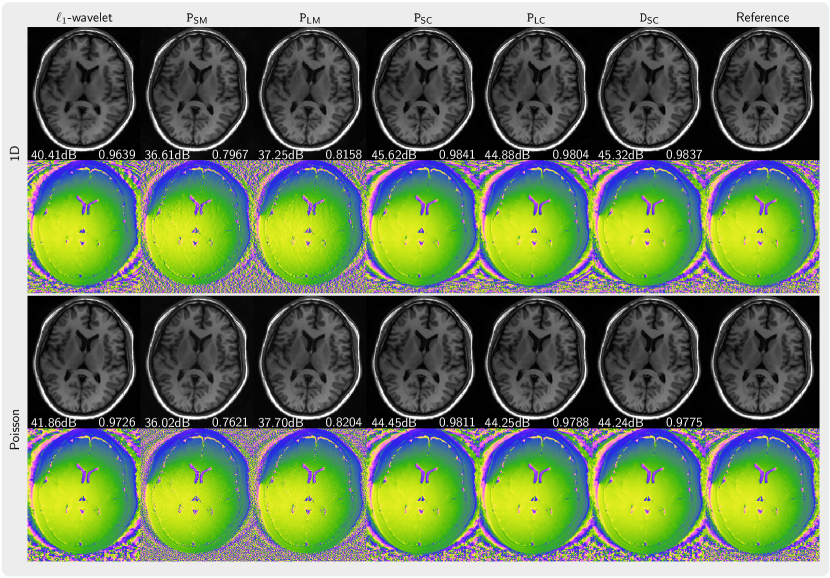
Figure 3: Comparison of images reconstructed using PICS using the priors P_SM, P_LM, P_SC, P_LC, D_SC in comparison to an $\ell_{1}$-wavelet reconstruction and a reference. The top two rows (1D) present the results for 5-fold acceleration along phase-encoding direction with 30 calibration lines. The bottom two rows (Poisson) show the results using a Poisson-disc acquisition of 8.2x-undersampling. PSNR and SSIM values are shown in white text.

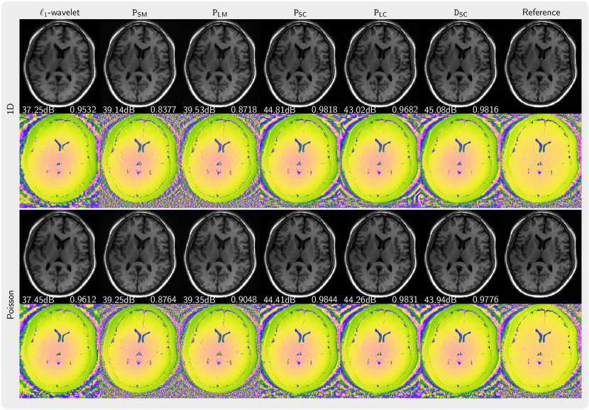
Figure 4: Comparison of images reconstructed using NLINV using the priors P_SM, P_LM, P_SC, P_LC, D_SC in comparison to an $\ell_{1}$-wavelet reconstruction and a reference. The top two rows (1D) present the results for 5-fold acceleration along phase-encoding direction with 30 calibration lines. The bottom two rows (Poisson) show the results using a Poisson-disc acquisition of 8.2x-undersampling. PSNR and SSIM values are shown in white text.

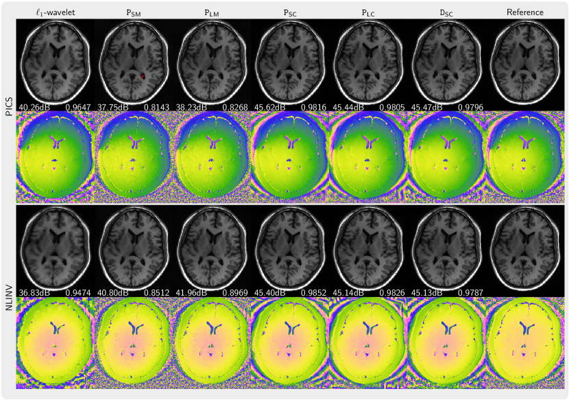
Figure 5: Comparison of images reconstructed using NLINV and PICS using the priors P_SM, P_LM, P_SC, P_LC, D_SC for a 2 $\times$ 3 sampling pattern in comparison to an $\ell_{1}$-wavelet reconstruction and a reference. PSNR and SSIM values are shown in white text. Artifacts (red arrow) are introduced by the priors trained on magnitude images reconstructed with PICS.

8.2 The influence of the size of dataset

Figure 6 presents the images regularized by the priors (P_SC and P_LC) trained on small and large datasets, respectively. When using PICS with the prior P_SC artifacts become apparent in the background and in the brain, whereas no such artifacts are observed when applying the prior P_LC. Furthermore, image details appear to be better preserved with high undersampling for the prior P_LC.

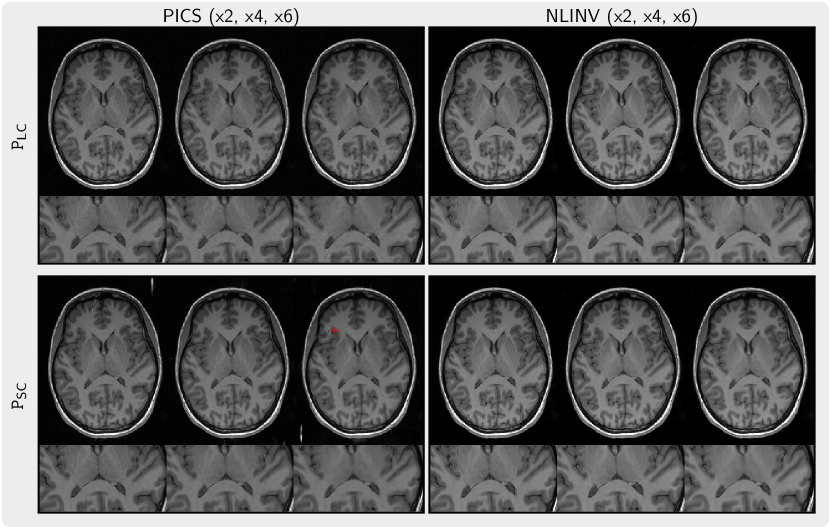
Figure 6: Comparison of images reconstructed with PICS (left) and NLINV (right) using priors P_SC (top) and P_LC (bottom) trained on small and large datasets. We observed artifacts (red arrow) when using PICS with the prior P_SC trained on the small dataset. The images in each column are reconstructed from k-space undersampled with factors ranging from 2 to 6 (left to right).

These observations can be confirmed quantitatively. We display the three sets of PSNR and SSIM metrics for $\ell_{2}$, P_SC, and P_DC with boxplots in Figure 7 for 4x and 6x undersampling relative to a reconstruction from 2x undersampled k-space and using P_LC. Here, the $\ell_{2}$-regularization serves as a baseline reconstruction which is not influenced by the properties of a learned prior. For the P_LC prior learned from a large dataset there are only a few outliers above the average when using PICS and NLINV. However, when using the P_SC prior learned from a small dataset there are many outliers below the average, especially when the undersampling factor is high in the case of PICS.

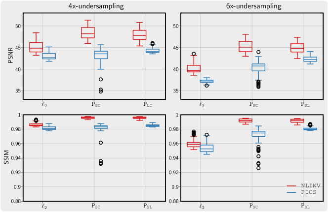
Figure 7: PSNR (top) and SSIM (bottom) metrics for images reconstructed with PICS (blue) and NLINV (red) when using $\ell_{2}$-regularization and when using the priors P_SC and P_LC for 4x (left) and 6x (right) undersampling relative to a reconstruction from 2x undersampled k-space and using P_LC.

8.3 3D reconstruction using diffusion priors

As an example, Figure 8 presents three slices in the sagittal, axial, and coronal planes for a 3D volume reconstructed using the diffusion prior D_SC using PICS and NLINV in comparison to $\ell_{1}$-wavelet regularization and a reconstruction by coil combination of Fourier-transformed fully-sampled k-space data. By visual inspection, the $\ell_{1}$-regularized images appear to have reduced sharpness compared to the images regularized by the diffusion prior D_SC while also having more noise.

Figure 9 shows the results from the evaluation by clinical readers. The diffusion prior D_SC outperforms $\ell_{1}$-wavelet regularization leveraging the learned knowledge. Here, D_SC demonstrates better performance when using PICS method compared to NLINV method. With the relatively high acceleration factor of 8.2 used, none of the reconstructions matches the quality of the reference. The images reconstructed using D_PC were very close to those using D_SC and are not shown.

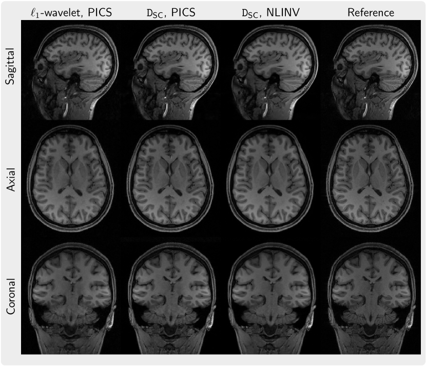
Figure 8: Slices in three orientations (Sagittal, Axial, Coronal, from top to bottom) from a 3D volume reconstructed using PICS from 8.2x-undersampled k-space with Poisson-disc sampling with $\ell_{1}$-wavelet regularization and the diffusion prior D_SC and using NLINV with diffusion prior D_SC (from left to right).

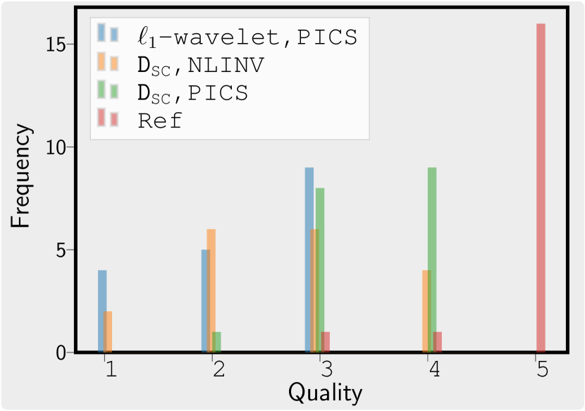
Figure 9: Blind evaluation by three clinicians of the volumes that are reconstructed with PICS using $\ell_{1}$-wavelet regularization, PICS with diffusion prior D_SC, NLINV with the diffusion prior, and using coil combination of Fourier-transformed fully-sampled k-space data. The grading scale ranges from 5 (excellent) to 1 (bad).

9 Discussion

A practical workflow was presented for extracting prior information from a set of magnitude-only images. It starts with the preparation of the training dataset, then followed by the generative modelling of complex-valued images and ends with the application of generative priors for regularization in image reconstruction. The effectiveness of the prior in boosting image quality was assessed by clinicians. Different aspects of this work are discussed below.

To exploit the information in magnitude-only images, the prediction of phase maps using an U-net was reported in Ref. Luo__2022a. Different to that, we prepared a training dataset of phase-augmented images through conditional generation using a complex diffusion prior that is first trained on a small dataset of complex-valued images. The prior trained on a large dataset of phase-augmented images exhibits high robustness, as shown in Figure 7. The proposed approach will allow us to leverage the information in the large number of DICOM images already available in the archives of radiology departments.

In Ref. Deveshwar_MDPI_BIOENG_2023, the authors applied a conditional generative adversarial network (GAN) to produce phase maps based on magnitude images and then used them to synthesize k-space data. They reported the comparable performance to raw k-space data when the synthetic k-space data were utilized to train a variational network⁶ for reconstruction. However, this still required running ESPIRiT on prior ground truth data from fastMRI³⁹ to obtain sensitivity maps for simulations. Ref. Zijlstra__2023 expanded this idea by generating coil sensitivity phase maps based on magnitude images. This was achieved through a three-stage approach, involving the generation of low-resolution coil sensitivity phase maps based on magnitude images with a GAN, upsampling of low-resolution maps to high-resolution ones, and transformation of the coil images to k-space data. Our work proposes a simple and less computationally intensive approach based on phase augmentation using a generic diffusion prior trained on complex-valued images. The advantage of this framework is that the learned prior is independent of k-space sampling patterns and coil sensitivities, and that it can be used as a regularization term in conventional reconstruction algorithms.

Training a prior is computationally expensive. For example, it took around 18 minutes to train P_LC per epoch through data parallelism using three A100 80G GPUs (Nvidia Corporation, Santa Clara, CA, USA). In contrast, use of the prior in conventional reconstruction algorithms is computationally efficient. While previous reports indicate that up to 2000 evaluations of a diffusion prior are needed for reconstructing a single image¹⁴, the number of evaluations required for a conventional linear reconstruction algorithm as used in this work is only about 100.

10 Conclusion

This work focuses on how to extract prior knowledge from existing magnitude-only image datasets using phase augmentation with generative models. The extracted prior knowledge is then applied as regularization in image reconstruction. The effectiveness of this approach in improving image quality is systematically evaluated across different settings. Our findings stress the importance of incorporating phase information and leveraging large datasets to raise performance and reliability of generative priors for MRI reconstruction.

11 Data Availability

In the spirit of reproducible research, the code used to preprocess the dataset and to generate complex-valued images by phase augmentation using the diffusion prior, and the shell scripts for the reconstruction are made available in our repository. The Python library spreco used to train priors is available in this repository. Pre-trained models are made available at Zenodo. We refer readers to the webpage of our repository for additional information on the released materials.

12 Acknowledgement

We acknowledge funding by the "Niedersächsisches Vorab" funding line of the Volkswagen Foundation.

References

- 1 Lustig M., Donoho D., Pauly J. M.. Sparse MRI: The application of compressed sensing for rapid MR imaging. Magn. Reson. Med.. 2007;58(6):1182–1195.
- 2 Block K. T., Uecker M., Frahm J.. Undersampled radial MRI with multiple coils. Iterative image reconstruction using a total variation constraint. Magn. Reson. Med.. 2007;57(6):1086–1098.
- 3 Vasanawala Shreyas S., Alley Marcus T., Hargreaves Brian A., Barth Richard A., Pauly John M., Lustig Michael. Improved Pediatric MR Imaging with Compressed Sensing. Radiology. 2010;256(2):607-616.
- 4 Feng Li, Benkert Thomas, Block Kai Tobias, Sodickson Daniel K., Otazo Ricardo, Chandarana Hersh. Compressed sensing for body MRI. Journal of Magnetic Resonance Imaging. 2017;45(4):966-987.
- 5 Yang Yan, Sun Jian, Li Huibin, Xu Zongben. Deep ADMM-Net for Compressive Sensing MRI. In: Advances in Neural Information Processing SystemsCurran Associates, Inc.; 2016.
- 6 Hammernik Kerstin, Klatzer Teresa, Kobler Erich, et al. Learning a variational network for reconstruction of accelerated MRI data. Magn. Reson. Med.. 2017;79(6):3055-3071.
- 7 Yaman Burhaneddin, Hosseini Seyed Amir Hossein, Moeller Steen, Ellermann Jutta, Uğurbil Kâmil, Akçakaya Mehmet. Self-supervised learning of physics-guided reconstruction neural networks without fully sampled reference data. Magnetic Resonance in Medicine. 2020;84(6):3172-3191.
- 8 Blumenthal Moritz, Luo Guanxiong, Schilling Martin, Haltmeier Markus, Uecker Martin. NLINV-Net: Self-Supervised End-2-End Learning for Reconstructing Undersampled Radial Cardiac Real-Time Data. In: Proc. Intl. Soc. Mag. Reson. Med.:0499; 2022; London, UK.
- 9 Tezcan Kerem C, Baumgartner Christian F, Luechinger Roger, Pruessmann Klaas P, Konukoglu Ender. MR image reconstruction using deep density priors. IEEE transactions on medical imaging. 2019;38(7):1633-1642.
- 10 Liu Qiegen, Yang Qingxin, Cheng Huitao, Wang Shanshan, Zhang Minghui, Liang Dong. Highly undersampled magnetic resonance imaging reconstruction using autoencoding priors. Magnetic Resonance in Medicine. 2020;83(1):322-336.
- 11 Luo Guanxiong, Zhao Na, Jiang Wenhao, Hui Edward S., Cao Peng. MRI reconstruction using deep Bayesian estimation. Magn. Reson. Med.. 2020;84(4):2246–2261.
- 12 Luo Guanxiong, Blumenthal Moritz, Heide Martin, Uecker Martin. Bayesian MRI reconstruction with joint uncertainty estimation using diffusion models. Magn. Reson. Med.. 2023;90(1):295-311.
- 13 Jalal Ajil, Arvinte Marius, Daras Giannis, Price Eric, Dimakis Alexandros G, Tamir Jon. Robust Compressed Sensing MRI with Deep Generative Priors. In: Ranzato M., Beygelzimer A., Dauphin Y., Liang P.S., Vaughan J. Wortman, eds. Advances in Neural Information Processing Systems:14938–14954Curran Associates, Inc.; 2021.
- 14 Chung Hyungjin, Ye Jong Chul. Score-based diffusion models for accelerated MRI. Medical Image Analysis. 2022;80:102479.
- 15 Luo Guanxiong, Blumenthal Moritz, Wang Xiaoqing, Uecker Martin. All you need are DICOM images. In: Proc. Intl. Soc. Mag. Reson. Med.:1510; 2022; London, UK.
- 16 Luo Guanxiong, Wang Xiaoqing, Roeloffs Volkert, Tan Zhengguo, Uecker Martin. Joint estimation of coil sensitivities and image content using a deep image prior. In: Proc. Intl. Soc. Mag. Reson. Med.:280; 2021; Virtual Conference.
- 17 Ying L., Xu D., Liang Z.-P.. On Tikhonov regularization for image reconstruction in parallel MRI. In: The 26th Annual International Conference of the IEEE Engineering in Medicine and Biology Society:1056-1059; 2004.
- 18 Ying L., Sheng J.. Joint image reconstruction and sensitivity estimation in SENSE (JSENSE). Magn. Reson. Med.. 2007;57(6):1196–1202.
- 19 Uecker M., Hohage T., Block K. T., Frahm J.. Image reconstruction by regularized nonlinear inversion-joint estimation of coil sensitivities and image content. Magn. Reson. Med.. 2008;60(3):674–682.
- 20 Uecker M., Block K. T., Frahm J.. Nonlinear Inversion with L1-Wavelet Regularization - Application to Autocalibrated Parallel Imaging. In: Proc. Intl. Soc. Mag. Reson. Med.:1479; 2008; Toronto.
- 21 Knoll F., Clason C., Bredies K., Uecker M., Stollberger R.. Parallel imaging with nonlinear reconstruction using variational penalties. Magn. Reson. Med.. 2012;67(1):34–41.
- 22 Romano Yaniv, Elad Michael, Milanfar Peyman. The Little Engine That Could: Regularization by Denoising (RED). SIAM J. Img. Sci.. 2017;10(4):1804–1844.
- 23 Salimans Tim, Karpathy Andrej, Chen Xi, Kingma Diederik P.. PixelCNN++: Improving the PixelCNN with Discretized Logistic Mixture Likelihood and Other Modifications. In: 5th International Conference on Learning Representations, ICLR Toulon, FranceOpenReview.net; 2017.
- 24 Sohl-Dickstein Jascha, Weiss Eric, Maheswaranathan Niru, Ganguli Surya. Deep Unsupervised Learning using Nonequilibrium Thermodynamics. In: Bach Francis, Blei David, eds. Proceedings of the 32nd International Conference on Machine Learning Proceedings of Machine Learning Research, vol. 37: :2256–2265PMLR; 2015; Lille, France.
- 25 Song Yang, Sohl-Dickstein Jascha, Kingma Diederik P, Kumar Abhishek, Ermon Stefano, Poole Ben. Score-Based Generative Modeling through Stochastic Differential Equations. In: International Conference on Learning Representations; 2021.
- 26 Beck A., Teboulle M.. A Fast Iterative Shrinkage-Thresholding Algorithm for Linear Inverse Problems. SIAM J. Img. Sci.. 2009;2(1):183–202.
- 27 Venkatakrishnan Singanallur V., Bouman Charles A., Wohlberg Brendt. Plug-and-Play priors for model based reconstruction. In: 2013 IEEE Global Conference on Signal and Information ProcessingIEEE; 2013.
- 28 Di Martino A., Yan C-G, Li Q., et al. The autism brain imaging data exchange: towards a large-scale evaluation of the intrinsic brain architecture in autism. Molecular Psychiatry. 2014;19(6):659–667.
- 29 Di Martino Adriana, O’connor David, Chen Bosi, et al. Enhancing studies of the connectome in autism using the autism brain imaging data exchange II. Scientific Data. 2017;4:170010.
- 30 Brett Matthew, Markiewicz Christopher J., Hanke Michael, et al. nipy/nibabel: 5.1.0. 2023.
- 31 Pascal Vincent. A Connection Between Score Matching and Denoising Autoencoders. Neural Computation. 2011;23(7):1661-1674.
- 32 Song Yang, Ermon Stefano. Generative Modeling by Estimating Gradients of the Data Distribution. In: Wallach Hanna M., Larochelle Hugo, Beygelzimer Alina, d’Alché-Buc Florence, Fox Emily B., Garnett Roman, eds. Advances in Neural Information Processing Systems 32: Annual Conference on Neural Information Processing Systems 2019, NeurIPS 2019, December 8-14, 2019, Vancouver, BC, Canada:11895–11907; 2019.
- 33 Ho Jonathan, Jain Ajay, Abbeel Pieter. Denoising Diffusion Probabilistic Models. In: Larochelle H., Ranzato M., Hadsell R., Balcan M.F., Lin H., eds. Advances in Neural Information Processing Systems:6840–6851Curran Associates, Inc.; 2020.
- 34 Lin Guosheng, Milan Anton, Shen Chunhua, Reid Ian. RefineNet: Multi-Path Refinement Networks for High-Resolution Semantic Segmentation. arXiv. 2016;.
- 35 Uecker M., Ong F., Tamir J. I., et al. Berkeley advanced reconstruction toolbox. In: Proc. Intl. Soc. Mag. Reson. Med.:2486; 2015; Toronto.
- 36 Blumenthal Moritz, Luo Guanxiong, Schilling Martin, Holme H. Christian M., Uecker Martin. Deep, deep learning with BART. Magn. Reson. Med.. 2023;89(2):678-693.
- 37 Uecker M., Lai P., Murphy M. J., et al. ESPIRiT—an eigenvalue approach to autocalibrating parallel MRI: where SENSE meets GRAPPA. Magn. Reson. Med.. 2014;71(3):990–1001.
- 38 Deveshwar Nikhil, Rajagopal Abhejit, Sahin Sule, Shimron Efrat, Larson Peder E. Z.. Synthesizing Complex-Valued Multicoil MRI Data from Magnitude-Only Images. Bioengineering. 2023;10(3).
- 39 Zbontar Jure, Knoll Florian, Sriram Anuroop, et al. fastMRI: An Open Dataset and Benchmarks for Accelerated MRI. arXiv. 2019;.
- 40 Zijlstra Frank, While Peter T. Deep-learning-based transformation of magnitude images to synthetic raw data for deep-learning-based image reconstruction. In: Proc. Intl. Soc. Mag. Reson. Med.:0825; 2023; Toronto, Canada.