On the stability around Chariklo and the confinement of its rings

Abstract

Context. Chariklo has two narrow and dense rings, C1R and C2R, located at 391 km and 405 km, respectively.

Aims. In the light of new stellar occultation data, we study the stability around Chariklo. We also analyse three confinement mechanisms, to prevent the spreading of the rings, based on shepherd satellites in resonance with the edges of the rings.

Methods. This study is made through a set of numerical simulations and the Poincaré surface of section technique.

Results. From the numerical simulation results we verify that, from the current parameters referring to the shape of Chariklo, the inner edge of the stable region is much closer to Chariklo than the rings. The Poincaré surface of sections allow us to identify the first kind periodic and quasi-periodic orbits, and also the resonant islands corresponding to the 1:2, 2:5, and 1:3 resonances. We construct a map of $a_{eq}$ versus $e_{eq}$ space which gives the location and width of the stable region and the 1:2, 2:5, and 1:3 resonances.

Conclusions. We found that the first kind periodic orbits family can be responsible for a stable region whose location and size meet that of C1R, for specific values of the ring particles’ eccentricities. However, C2R is located in an unstable region if the width of the ring is assumed to be about 120 m. After analysing different systems we propose that the best confinement mechanism is composed of three satellites, two of them shepherding the inner edge of C1R and the outer edge of C2R, while the third satellite would be trapped in the 1:3 resonance.

1 Introduction

The amazing rings of Saturn were discovered in the seventeen century by Galileo Galilei, although he died before knowing he had discovered a unique planetary ring system. Only three centuries later, the rings around the giant planets Jupiter, Uranus and Neptune were revealed by the spacecraft Voyager I and II and by stellar occultations.

A new class of objects sheltering a ring system was discovered in 2014 by Braga Ribas and colleagues [2014, BR14 hereafter]BragaRibas2014 through stellar occultation. They discovered a ring system around the largest Centaur (10199) Chariklo. This Centaur object could originate in the trans-Neptunian region and could be deflected to the Centaur region probably due to a close encounter with Neptune within the last 20 Myr (Wood et al., 2017).

The two dense rings, 2013C1R and 2013C2R, in orbit around Charilko are very narrow rings with widths of about 7 km and 3 km and optical depths of 0.4 and 0.06, respectively (BR14). They are located very close to Chariklo, their orbital radii are 391 km and 405 km. BR14 speculated three scenarios for the origin of the two rings, one of them relies on a collision between a satellite onto the surface of Chariklo. This collision could release material from Chariklo and forms the rings, or the impactor satellite could be destroyed originating the rings.

Regarding the composition of the rings, Duffard et al. (2014) obtained that silicates, tholins and water ice may be present in C1R and C2R, while Sicardy (2020) claimed that the presence of icy water, shown in the spectrum of the rings, may be caused by Chariklo.

A set of five stellar occultations presented in Leiva et al. (2017) between 2013 and 2016 helped to constrain the size and shape of Chariklo. The shape of an object can help to analyse the dynamical behaviour that nearby particles can perform, and in this particular case, could help to understand the origin and evolution of the rings. They considered four possible models for Chariklo: a sphere with radius equal to $129$ km, a MacLaurin spheroid with about $a=b=143$ km and $c=96$ km, a triaxial ellipsoid with $a=157$ km, $b=132$ km and $c=102$ km, and a Jacobi ellipsoid with $a=157$ km, $b=139$ km and $c=86$ km, where $a$, $b$ and $c$ are the semi-axes. With the derived mass range for Chariklo of $6-8\times 10^{18}$ kg, they pointed out that the 1:3 resonance between the rotation of Chariklo and the orbital motion of the particles is at $408\pm 20$ km, close to the location of the rings.

A paper by Morgado et al. (2021) – M21 hereafter – presents new stellar occultation data obtained between 2017 and 2020. These new data helped to improve Chariklo and the rings parameters. The parameters of C1R and C2R can be consulted in Table 1. They also concluded that these rings may contain particles larger than $1\leavevmode\nobreak\ \mu$m in size. An important result concerns the shape of Chariklo, from these stellar occultations data Chariklo is consistent with a triaxial ellipsoid with semi-axes $a=143.8$ km, $b=135.2$ km and $c=99.1$ km (M21).

The relation between the inner ring of Chariklo and the 1:3 spin-orbit resonance (resonance between Chariklo’s rotation period and the mean motion of the particles) was explored in Madeira et al. (2022) by assuming Chariklo as a spherical body with a mass anomaly at its equator. Such an assumption is based on observational data that suggests the presence of topographic features in the Centaur (Sicardy et al., 2019). Through a set of Poincaré surface of sections, Madeira et al. (2022) obtain that the non-spherical shape of Chariklo is responsible for an unstable region extending from its surface to an orbital radius of $\sim$320 km, far inside the ring system. Despite the proximity between the 1:3 spin-orbit resonance and the inner ring, the authors verify that such resonance would be responsible for eccentricities $\sim 10^{-2}$, higher than expected for the ring particles. Their results show that Chariklo rings are probably associated with first kind orbits.

Several papers analysed the rings dynamics. El Moutamid et al. (2014) and Melita et al. (2017) discussed the possibility that the ring was formed from the disruption of an old satellite, which can occur if the satellite crosses the Roche limit of Chariklo. The location of the Roche limit depends on the physical parameters of both objects, and for this to match the current locations of the rings, the satellite must be porous, with a density much lower than Chariklo. In addition, the satellite must have a minimum radius of $\sim 7$ km (Melita et al., 2017). However, a problem with this hypothesis is the absence of mechanisms to bring the satellite to this limit. Tidal dissipation, the primary mechanism that could be responsible for this, is not a plausible option. Chariklo’s corotation radius is within the locations of the rings. Therefore a satellite beyond the Roche limit would migrate farther away from Chariklo unless it rotated much slower in the past.

Another possibility ruled out by Melita et al. (2017) is that the disruption is caused by a destructive impact of an old satellite with an external projectile, because the estimated timescale for such an event to occur is longer than Chariklo’s lifetime. The authors also analysed the impactor flux in the Chariklo region and conclude that the ring formation due to an impact of a projectile with Chariklo is improbable.

Pan & Wu (2016) proposed that the close encounter that brought Chariklo to the Centaur region would enormously increase its temperature, being responsible for the sublimation of CO material. They estimated that Chariklo re-accretes part of this material, while the rest settles in the equation plane after multiple collisions. The latter has dust sizes and mechanically sticks together, forming a material disk that spreads out and forms the Chariklo system. More data on the Chariklo composition are needed to verify if such a process can produce the amount of material observed in the rings.

Hyodo et al. (2016) propose that the ring material may have formed by the partial tidal disruption of Chariklo during an extreme close encounter. Their model assumed a differenciated Chariklo with an ice mantle and it was analysed using hydrodynamic simulations. According to them, the planet’s tidal effects instantly remove material from Chariklo’s surface. Over time, such material settles in the equatorial plane mainly within the Roche limit and viscously spreads out. Finally, the material outside the Roche limit accretes into moons that destructively collide with each other, forming the rings and shepherd satellites (Hyodo & Ohtsuki, 2015). This model has the advantage of explaining the ice composition of the rings (Duffard et al., 2014), while it does not require the presence of an old satellite. However, it does require extremely rare close encounters (Araujo et al., 2016; Wood et al., 2017). Furthermore, Chariklo composition is uncertain and more data is needed to verify the most plausible mechanism for the formation of Chariklo system.

While several relevant works analysed possible scenarios for the origin of Chariklo rings, our focus in this work is to analyse the stability of the region face to the new parameters obtained for Chariklo (M21) in order to verify if the rings are located in a stable region and/or close to a resonance. This analysis was performed through a set of numerical simulations and also through the powerful technique of the Poincaré surface of section. Furthermore, we explore several confinement models for constrain these rings.

Our paper is divided into 6 sections. Section 2 deals with the dynamical system and also presents the results obtained from the numerical simulations, while in section 3 the periodic and quasi-periodic orbits are studied in light of the Poincaré surface of sections. In section 4 we analyse the location of the rings in the $a_{eq}$ versus $e_{eq}$ map. In section 5 we discusses different confinement models to constrain the rings. Conclusions on this work is presented in section 6.

Table 1: The orbital radii, the width and the optical depth of both rings, C1R and C2R, are shown here. This table also includes the semi-axes ($a,b,$ and $c$), the mass and the rotation period of Chariklo (BR14; Leiva et al. (2017); M21).

	C1R	C2R
Orbital radii (km)	385.9	399.8
Width (km)	4.8-9.1	0.117
Optical depth	0.4	0.06
	Chariklo
${\rm a\times b\times c}$ (km)	143.8 $\times$ 135.2 $\times$ 99.1
Mass (kg)	${\rm 6.3\times 10^{18}}$
Rotation period (h)	7.004

2 Dynamical System

The equations of motion of a massless particle around Chariklo, considering a body-fixed frame (O$xy$) uniformly rotating with the same spin period of Chariklo, can be given by (Hu & Scheeres, 2004)

$$\ddot{x}-2\omega\dot{y}=\omega^{2}x+U_{x},$$ (1)

and

$$\ddot{y}+2\omega\dot{x}=\omega^{2}y+U_{y}$$ (2)

where $U_{x}$ and $U_{y}$ are the gravitational potential partial derivatives for Chariklo and $\omega$ is its spin velocity. Here, we assume Chariklo represented by a second degree and order gravity field. The oblateness ($C_{20}$) and the ellipticity ($C_{22}$) are gravitational potential coefficients whose values can be computed from the ellipsoidal semi-axes $(a,b,c)$ as (Balmino, 1994)

$$C_{20}=(2c^{2}-a^{2}-b^{2})/10{R_{e}}^{2}$$ (3)

and

$$C_{22}=(a^{2}-b^{2})/20{R_{e}}^{2}$$ (4)

where $a>b>c$ and $R_{e}=(a\,b\,c)^{1/3}$. The gravitational potential can be expressed as (Hu & Scheeres, 2004)

$$U(x,y)=\frac{\mu}{r}\left(1-\left(\frac{R_{e}}{r}\right)^{2}\left[\frac{C_{20}}{2}-\frac{3C_{22}}{r^{2}}(x^{2}-y^{2})\right]\right),$$ (5)

where $\mu$ is the gravity parameter and $r=\sqrt{x^{2}+y^{2}}$. Note that the physical major axis of the body is aligned with the O$x$ axis of the rotating system.

In this section the system (Chariklo-ring particle) described by Equations (1) and (2) will be analysed into two different ways: i) through a set of numerical simulation and ii) through the technique of Poincaré surface of sections.

2.1 Numerical Results

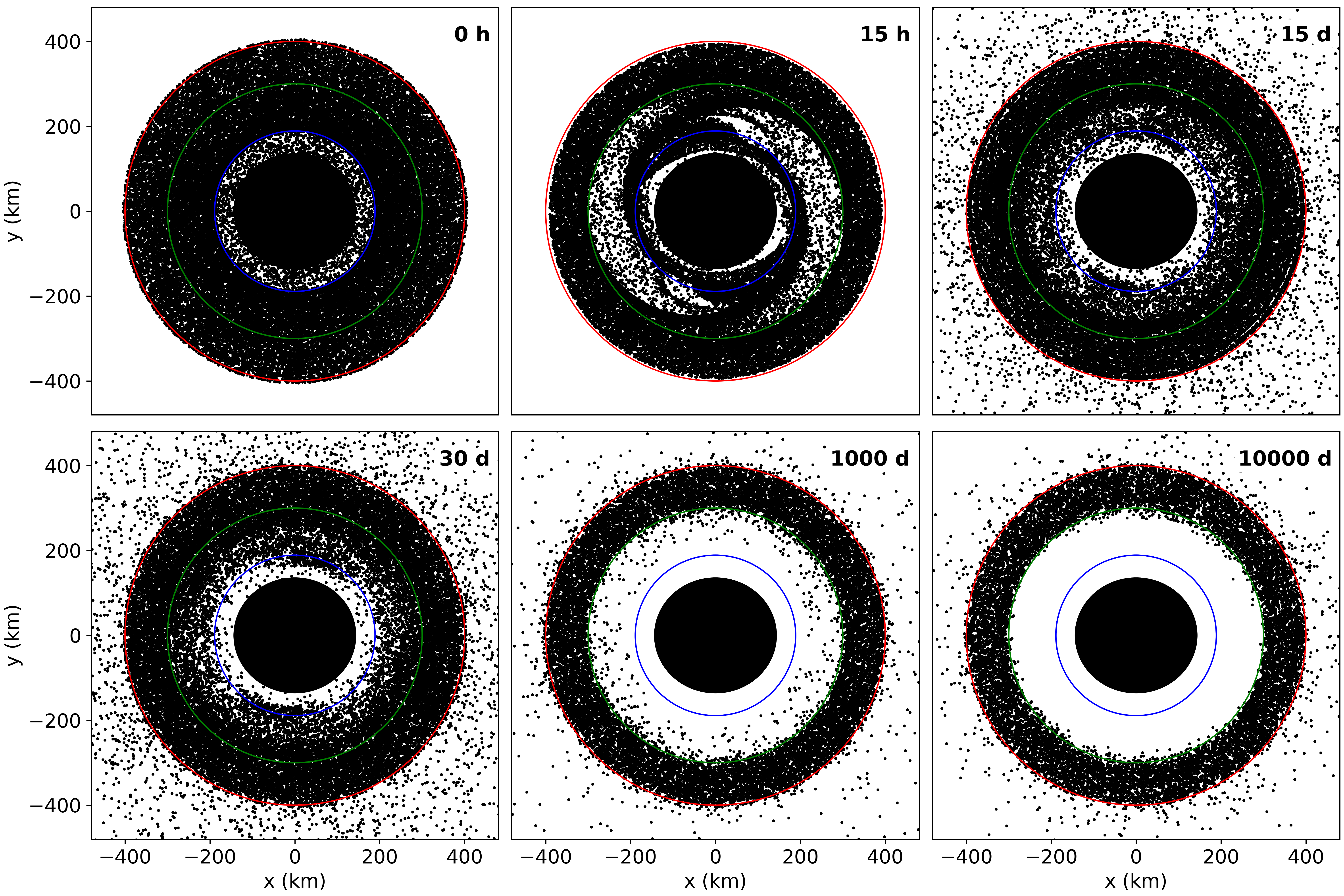
Figure 1: These snapshots show the orbital evolution (in the rotational frame with Chariklo) of a set of test particles under the effects of $C_{20}$ and $C_{22}$, the gravitational coefficients of Chariklo (black circle). The blue circle shows the location of the corotation radius, while the green and red circles show the semi-major axes of the 1:2 and 1:3 resonances, respectively.

Our first goal is to find the inner edge of the stable region around Chariklo. For that we performed numerical simulations using a disc of non-interacting massless particles moving around Chariklo. In the gravitational potential of Chariklo we take into account the contributions of its oblateness ($J_{2}$) and ellipticity ($C_{22}$). After some changes to include the $C_{22}$ contribution in the equations of motion (Celletti et al., 2017), a N-body simulation in the Rebound package (Rein & Liu, 2012) with the IAS15 integrator (Rein & Spiegel, 2015) was used to numerically integrate the system.

The particles were distributed with random values of the true longitude between $0^{\circ}-360^{\circ}$ from the equivalent radius ($R_{eq})$ of the central body ($\approx$ 124 km) to the position of its main ring ($\approx$ 400 km). Knowing that the inner edge of the disc suffers large perturbations due to the azimuthal asymmetry of the central body, the amount of initial particles in this region is low, since most of them will be ejected or will collide with the central body, consuming unnecessary computing resources. This region that extends from the $R_{eq}$ to the corotational radius ($\approx$ 189 km, Sicardy et al., 2019) has a set of 1000 particles, while the remaining part of the disc is composed by 40000 particles.

All adopted parameters of Chariklo are given in Table 1. A collision is detected when the orbital radius of the particle is smaller than the equivalent radius of Chariklo, while those particles with a semi-major axis larger than five times the orbital radius of the main ring are removed from the system. The numerical simulation has been carried out for 10000 years.

Figure 1 shows the initial positions of the particles (0 h), and the positions after 15 hours, 15 days (15 d), 30 days, 1000 days and after the complete time span of the numerical simulation (10,000 days). One day corresponds approximately to 3.43 Chariklo’s rotation period. The blue circle shows the corotation semi-major axis, the green and the red circles show the location of the 1:2 and 1:3 spin-orbit resonances, respectively.

Under the effects of Chariklo’s non-axisymmetric gravity field, the particles are removed from the inner region through collisions with Chariklo and ejections from the system. As can be seen, after 10000 days, Chariklo’s elongation clears a region up to the location of the 1:2 spin-orbit resonance (green circle), where the stable region begins.

This result shows the size of the unstable region for the recent refined physical parameters of Chariklo [M21]. Comparing our results with those presented by Sicardy et al. (2019), there is a difference in the location of the inner edge of the stable region. This is mainly due to the assumed value of $C_{22}$, which is derived from the semi-axes ($a$, $b$ and $c$). The value of $C_{22}$ obtained from the semi-axes given by M21 is almost half of the value assumed by Sicardy et al. (2019), which can explain the decreasing in the unstable region.

2.2 Poincaré Surface of Section

It is known that the system has an integral of motion, the Jacobi constant ($C_{j}$). This conserved quantity, given by (Hu & Scheeres, 2004)

$$C_{j}=\omega^{2}(x^{2}+y^{2})+2U(x,y)-\dot{x}^{2}-\dot{y}^{2}$$ (6)

is used in the construction of the Poincaré surface of section. In order to unequivocally determine a particle in the phase space it is necessary to have four elements: two for the position $(x,y)$ and two for the velocity $(\dot{x},\dot{y})$. Fixing a value for the Jacobi constant $C_{j}$ it becomes necessary to have just three of the four elements, for example, $x$, $y$ and $\dot{x}$. Defining the section as being $y=0$, all points of the trajectory that cross this section in a given direction ($\dot{y}_{0}<0$) can be plotted in the plane $(x,\dot{x})$, producing the Poincaré surface of section. Several works also used the Poincaré surface of section technique to study a two-body problem system with a central body with non-spherical distribution of mass (Scheeres et al., 1996; Jiang et al., 2016; Feng & Hou, 2017; Borderes-Motta & Winter, 2018; Winter et al., 2019; Madeira et al., 2022).

This is a numerical procedure where the equations of motion (1) and (2) were integrated using the Bulirsh-Stoer integrator (Bulirsch & Stoer, 1966). The Newton-Raphson method was used to obtain the points of the trajectory that cross the section defined by $y=0$, with an error of at most $10^{-13}$. For each Jacobi constant, $C_{j}$, we considered between 20 and 30 initial conditions. The choice of initial conditions is carried out into two stages:

• firstly, we distribute a set of initial conditions equally spaced on the O$x$ axis, with $x=0$ and $\dot{y}>0$. The $\dot{y}$ velocity is calculated using Equation 6. These first initial conditions can generate the chaotic regions, the family of the first type orbits and the families of resonant orbits that have islands passing through the $\dot{x}=0$ axis on the Poincaré surface of section.

• For the resonant orbits that do not have islands crossing the $\dot{x}=0$ axis in the Poincaré surface of section, a second distribution of initial conditions equally spaced in $x\neq 0$ is needed. This distribution occurs in the region where the resonance is found in the Poincaré surface of section.

The results of a surface of section are geometrically interpreted in a simple way, since periodic orbits produce a number of fixed points, while quasi-periodic orbits generate islands (closed curves) around the fixed points. Points spread over an area of the section are identified as chaotic trajectories.

As a reminder, we consider the Jacobi ellipsoid shape model proposed by M21, see Table 1 . Since $C_{22}$ is different from zero, resonances between the spin of Chariklo and the orbital motion of the particle appear in the system.

The 1:3 spin-orbit resonance is of particular interest once it is close to the location of the ring (Leiva et al., 2017). Through the Poincaré surface of sections, we explored a wide range of $C_{j}$ values in order to identify the islands associated with the 1:3 resonance. These islands exist for $7.337\times 10^{-3}\,{\rm km}^{2}{\rm s}^{-2}<C_{j}<7.525\times 10^{-3}\,{\rm km}^{2}{\rm s}^{-2}$. The 1:3 resonance is shown in the plots of Figure 2 (in green and purple colours).

It is important to notice that, formally, this 1:3 resonance is a fourth order 2:6 resonance, since the potential (Equation 5) is invariant under a rotation of $\pi$ (Sicardy et al., 2019; Sicardy, 2020), which is a doubled resonance that produces a pair of periodic orbits and their associated quasi-periodic orbits. Consequently, there are two pairs of mirrored sets of islands in the Poincaré surface of sections (one pair in green and other in purple), since each one of the periodic orbits generates two fixed points with their islands of quasi-periodic orbits around them. From now on we will refer to 1:3 resonance, instead of 2:6 resonance. It is also valid for the 1:2 (2:4) resonance.

Once this resonance is doubled in the phase space, a separatrix appears between the two families of periodic/quasi-periodic orbits, producing a chaotic region whose size depends on the Jacobi constant value.

In the Poincaré surface of sections shown in Figure 2, pairs of islands in green and pairs of islands in purple indicate the quasi periodic orbits associated with the 1:3 resonance. For $C_{j}=7.337\times 10^{-3}\,{\rm km}^{2}{\rm s}^{-2}$ they are small and distant from the red islands centre. As the value of $C_{j}$ increases their size grows and gets closer to the red islands centre. The green and purple islands are bigger for $C_{j}\sim 7.374\times 10^{-3}\,{\rm km}^{2}{\rm s}^{-2}$, when they are near to the red islands. As the $C_{j}$ value keeps increasing, the 1:3 resonance islands start to reduce their sizes and get closer to the red islands centre, being surrounded by red islands ($C_{j}=7.525\times 10^{-3}\,{\rm km}^{2}{\rm s}^{-2}$). The evolution continues as they approach to the red islands centre, always getting smaller. A family of periodic orbits of the first kind (Poincaré, 1895) is responsible for the red islands. This will be discussed in details in the following section.

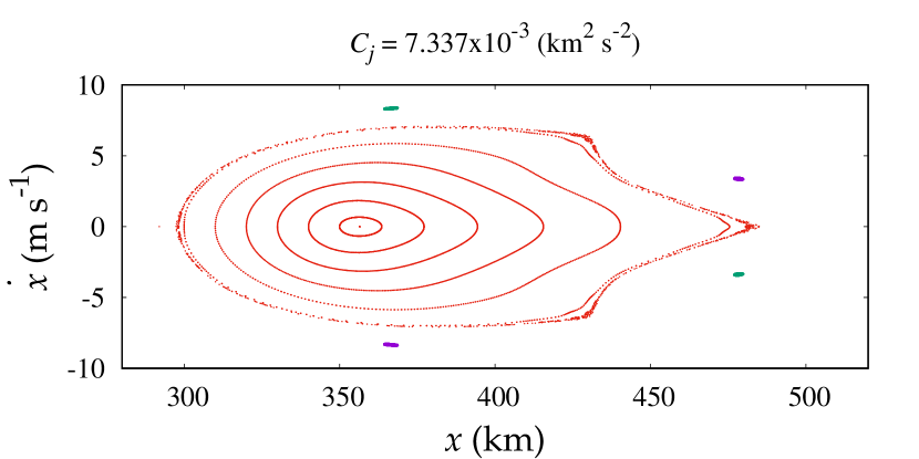
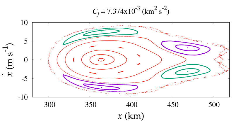
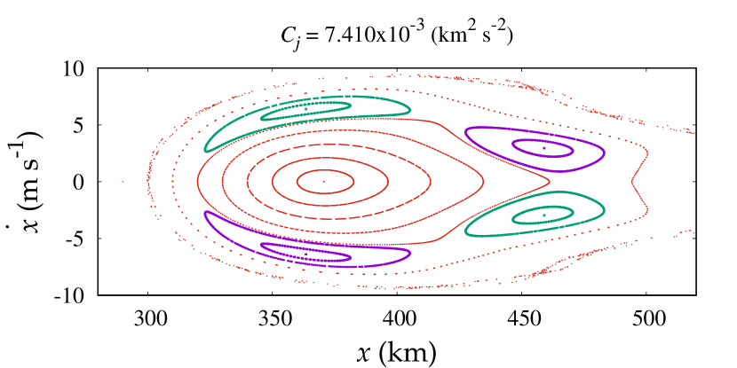
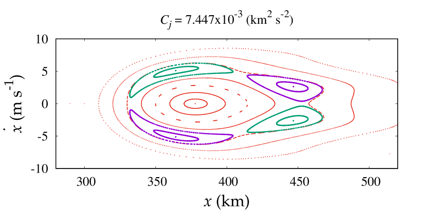
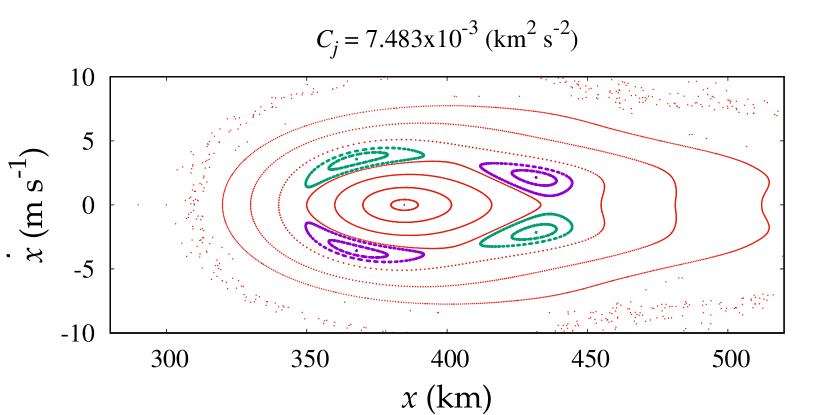
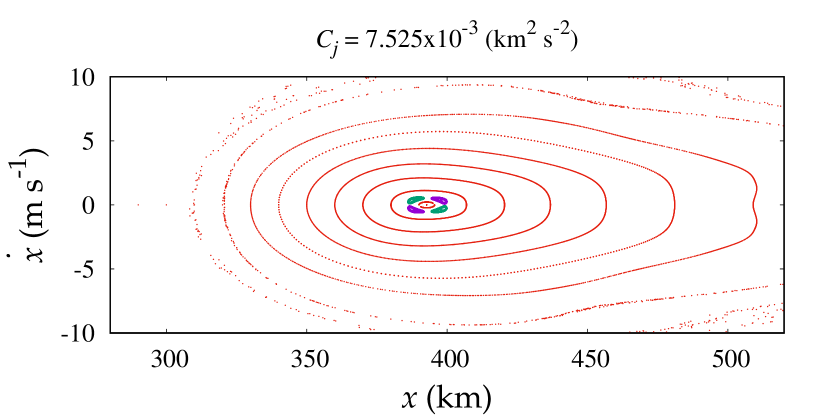
Figure 2: Set of Poincaré surface of sections covering the whole 1:3 resonance evolution. There are two families of 1:3 resonant periodic orbits indicated with different colours, purple and green. A family of first kind periodic orbits is responsible for the quasi-periodic orbits shown as red islands.

3 Periodic Orbits

Traditionally, periodic orbits in the planar, circular, restricted three-body problem have been classified as periodic orbits of the first kind and of the second kind (Poincaré, 1895; Szebehely, 1967). The so-called resonant periodic orbits are the periodic orbits of the second kind, whose particles are in eccentric orbits in a mean motion resonance. The less well known are the periodic orbits of the first kind, which are those originated from particles initially in circular orbits in the unperturbed system (simple two-body problem).

Families of periodic orbits of the first kind have being studied in several systems. For example, in the restricted three-body problem, Broucke (1968) considered the Earth-Moon case, Winter & Murray (1997) studied in the Sun-Jupiter system, and Giuliatti Winter et al. (2013) found them in the Pluto-Charon system. Now, considering the restricted two-body problem, where the primary is a rotating non-spherical triaxial body, Borderes-Motta & Winter (2018) and Winter et al. (2019) showed examples of both kinds of periodic orbits.

From the set of Poincaré surface of sections shown in Figure 2, the dynamical structure of the region where are located the rings of Chariklo is determined by two families of 1:3 resonant periodic orbits (in purple and in green colours) and by a family of periodic orbits of the first kind (in red colour). We will explore some features of these periodic orbits.

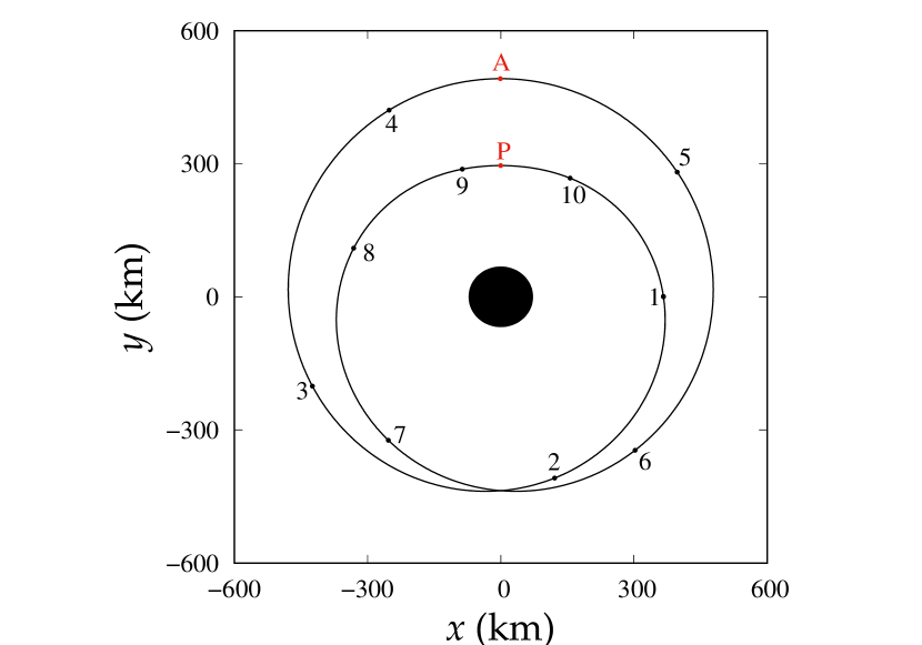
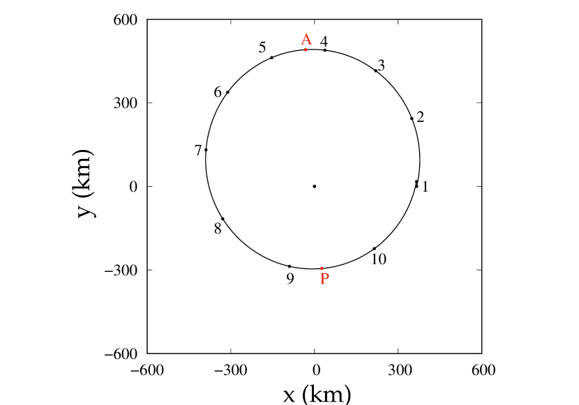
Figure 3: Example of a 1:3 resonant periodic orbit whose Jacobi constant value is $C_{j}=7.337\times 10^{-3}\,{\rm km}^{2}/{\rm s}^{2}$ and its period in the rotating frame is $T=21.01$ h. The points at the centre of the islands, in purple, shown in the Poincaré surface of section of Figure 2 (first plot) correspond to this periodic orbit. In the top plot is the trajectory in the rotating frame, while the trajectory in the inertial frame is shown in the middle plot. The temporal evolution of the orbital radius is shown in the bottom plot. The numbers in the top and middle plots show the locations equally spaced in time, indicating the time evolution of the trajectory. The letters $P$ and $A$ indicate the location of the pericentre and the apocentre, respectively.

Figure 4: Example of a first kind periodic orbit with $C_{j}=7.337\times 10^{-3}\,{\rm km}^{2}/{\rm s}^{2}$ and the period of the periodic orbit in the rotating frame is $T=11.5$ h. The point at the centre of the islands in red, shown in the Poincaré surface of section of Figure 2 (first plot), corresponds to this periodic orbit. In the top plot is shown the trajectory in the rotating frame, while the trajectory in the inertial frame is in the middle plot. The temporal evolution of the orbital radius is shown in the bottom plot. The numbers in the top and middle plots show the locations equally spaced in time, indicating the time evolution of the trajectory.

Since the 1:3 resonance is doubled, we selected just one of the resonant periodic orbits to study. The other orbit is a mirrored image of this one. Considering the Jacobi constant $C_{j}=7.337\times 10^{-3}\,{\rm km}^{2}{\rm s}^{-2}$, in Figure 3 is shown a 1:3 resonant periodic orbit. This is the periodic orbit shown in the Poincaré surface of section of Figure 2 (first plot), which corresponds to the points at the centre of the islands shown in purple.

The top plot shows the trajectory in the rotating frame. The numbers indicate the time evolution of the trajectories and show the locations equally spaced in time. In the rotating frame the trajectory is retrograde and symmetric with respect to the line $x=0$, where are located the pericentre ($P$) and apocentre ($A$) of the trajectory. The period of this periodic orbit is $T=21.01$ h, which is very close to three periods of rotation of Chariklo. In the inertial frame, the trajectory is prograde (middle). The temporal evolution of the orbital radii of the trajectory (bottom) also helps to visualise the trajectory shape.

The angle of the 1:3 resonance is given by $\phi_{1:3}=\lambda_{C}-3\lambda+2\varpi$, where $\varpi$ and $\lambda$ are the longitude of the pericentre and mean longitude of the particle, respectively, and $\lambda_{C}$ is the orientation angle of Chariklo. For all resonant trajectories shown in Figure 2, the resonant angle oscillates around $\pi$ (orbits in purple) or $-\pi$ (orbits in green).

In Figure 4 is presented an example of a first kind periodic orbit, with $C_{j}=7.337\times 10^{-3}\,{\rm km}^{2}{\rm s}^{-2}$. Through a careful analysis, we verified that the trajectory of a particle in the rotating frame always follows a shape similar to the shape of Chariklo. The closest points of the trajectory (indicated by numbers 2 and 4) are aligned with the short axis of Chariklo, while the furthest points of the trajectory (indicated by numbers 1 and 3) are aligned with its long axis.

The period of this periodic orbit is $T=11.5$ h, a little more than 1.5 times the spin period of Chariklo. Note that, at the same time it completes one period in the rotating frame, the trajectory completed only a little more than half of its orbit around Chariklo in the inertial frame. The temporal evolution of the radial distance (bottom plot of Figure 4) clearly shows that the trajectory has a pair of minima and a pair of maxima. This trajectory is not a usual Keplerian ellipse, with the central body at one of the foci. Actually, the trajectory is like an ellipse with the central body at its centre.

A comparison between the radial amplitudes of oscillation of this periodic orbit of the first kind (bottom plot of Figure 4) and the resonant periodic orbit given in the bottom plot of Figure 3 shows a huge difference. Note that the resonant periodic orbit shows a radial oscillation of more than 190 km while the periodic orbit of the first kind oscillates less than 1 km. Such difference will be analysed for the whole set of periodic orbits in the next section.

A striking difference between a periodic orbit of the first kind and a resonant periodic orbit is that the period (in the rotating frame) of a periodic orbit of the first kind varies significantly, in a range that might cross several values that are commensurable without becoming resonant. The period of the periodic orbits in the rotating frame as a function of their Jacobi constant, $C_{j}$, is shown in Figure 5. Note that the resonant periodic orbits 1:3 (in purple) exist only nearby the period commensurable with the spin period of Chariklo, while the period of the periodic orbits of the first kind covers a wide range of values (red), crossing some periods that are commensurable with the spin period of Chariklo.

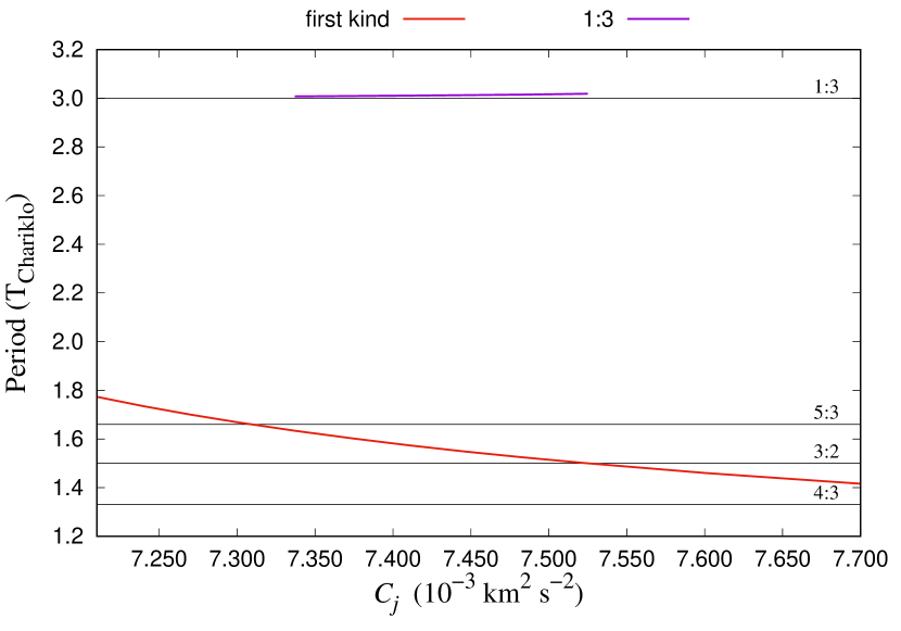
Figure 5: Period of the periodic orbits in the rotating frame as a function of their Jacobi constant, $C_{j}$. In red are the periods for the first kind periodic orbits, while in purple are the values for the 1:3 resonant periodic orbits. Some periods that are commensurable with Chariklo’s spin period ($T_{\rm Chariklo}$), in the rotating frame, are indicated by the black straight lines.

4 Location of the Rings

Following the approach developed by Winter et al. (2019), we look for a correlation between the locations and sizes of the rings of Chariklo and the locations of the stable regions associated with the periodic orbits analysed in the last section.

As seen in Figure 4, in the rotating frame, the first kind periodic orbits have an ellipsoidal shape with Chariklo at its centre, with a radial extent going from a minimum ($r_{\rm min}$) to a maximum ($r_{\rm max}$) radial distance from Chariklo. This same radial extent can be obtained by a Keplerian ellipse with a pair of equivalent semi-major axis and eccentricity ($a_{\rm eq},e_{\rm eq}$), where $a_{\rm eq}=(r_{\rm min}+r_{\rm max})/2$ and $e_{\rm eq}=1-(r_{\rm min}/a_{\rm eq})$ (Winter et al., 2019).

Adopting this same idea, each one of the rings of Chariklo can be represented by a set of Keplerian ellipses with equivalent semi-major axis $a_{\rm eq}$ and eccentricity $e_{\rm eq}$, covering the same radial extent of the ring. Figure 6a shows a comparison of this region covered by these Keplerian ellipses and our results on the stable region around Chariklo, adopting the Jacobi ellipsoid shape model proposed by M21. The pink colour refers to the region of periodic and quasi-periodic orbits of the first kind (red islands in the Poincaré surface of sections in Figure 2). This region is bounded by two red lines: bottom, which corresponds to the semi-major axis and eccentricity of the first kind periodic orbits, and upper, which refers to the quasi-periodic orbits of largest libration, for each value of $C_{j}$. The yellow, blue, and green regions correspond to the widths of the 1:2, 2:5, and 1:3 resonances, respectively. Resonance width limits are obtained by calculating the pair ($a_{eq}$, $e_{eq}$) of the quasi-periodic orbits with the largest libration for each value of $C_{j}$. The black dashed lines indicate the centre of each of these resonances.

Additionally, the dark blue and coral regions indicate the equivalent region covered by C1R and C2R, respectively. The width of each ring was derived from the observations (M21) and they are represented by dashed lines (we assumed the upper limit of C1R width provided by M21, $W=9.1$ km). A particle located on the inner or outer edge of the C1R can assume any values of the eccentricity and semi-major axis defined in the dark blue region which will guarantee that the width of C1R will be about 9 km (M21).

The width of the dark blue region changes due to the fact that a ring particle with a non-zero value of eccentricity needs to be located in a particular semi-major axis in order to keep the width of the ring (shown as dashed lines in dark blue and coral colours representing C1R and C2R, respectively). As the eccentricity of the particle increases, the values of the semi-major axis that this particle can be located decrease. For larger values of $e$ ($>0.015)$ the excursions of the ring particle will lead to a value larger than the width of the ring. Figure 6b shows a zoom of the C1R region, with the horizontal dotted lines placing the limits of C1R eccentricity obtained by M21, eccentricities equal to 0.005 and 0.022.

From a certain value of the eccentricity ($0.0006$), it can be noted that the dark blue region enters the stable region of the orbits of the first kind, indicating that the C1R particles need to have a minimum value of eccentricity to be located in a stable region. The upper limit of eccentricity (0.022), in turn, is outside the dark blue region. This value was obtained by M21 by adjusting the observed data from Chariklo centre, corresponding to the upper bound for a 3-sigma confidence level. For 1-sigma confidence level, the upper bound is 0.014, a value pretty similar to the maximum eccentricity in the dark blue region (0.012). Therefore, our equivalent region of stability is consistent with the observed location of C1R.

Note that if a particle on the outer/inner edge of a ring located in the 1:3 resonance region, for example, for the values $e=0.0205$ and $a=392.55$ km (bottom point of the green area), the radial excursion of the particle would be very large, about 16 km.

For C2R the situation is different. Since it has a very small width, around $0.117$ km (M21), the eccentricity of the particles must be very small ($<0.00013$). However, for C2R to be in a stable region (pink region), its eccentricity must be larger than 0.0006. Consequently, its width has to be larger than $\sim 120$ m (M21). This poses a problem with the stability of this ring.

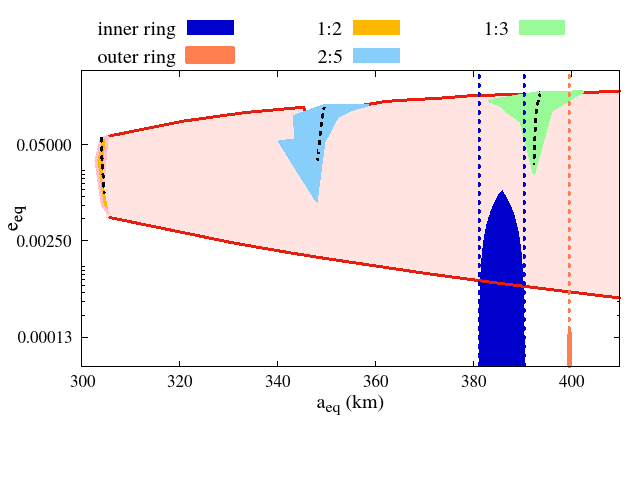
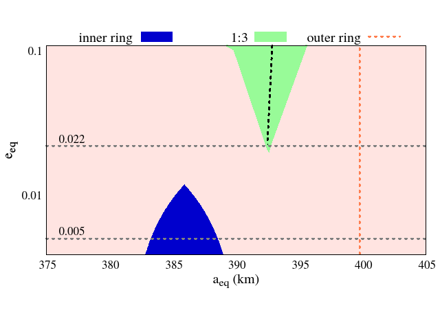
Figure 6: (a) Map of the stable region around Chariklo in $a_{eq}$ versus $e_{eq}$ space. The stable region indicated by the pink colour is due to the first kind orbits. This region is limited by two red lines: bottom, which corresponds to the semi-major axis and eccentricity of the first kind periodic orbits, and upper, which refers to quasi-periodic orbits. The yellow, blue, and green regions are related to 1:2, 2:5, and 1:3 resonances, respectively. Black dashed lines indicate the centres of each resonance, determined through the geometry of the resonant orbits. The dark blue and coral regions show the ranges ($a_{eq}$, $e_{eq}$) that correspond to the locations of the inner (C1R) and outer (C2R) rings of Chariklo, respectively. The dashed dark blue and coral lines show the edges of the rings. A zoom in the bottom plot (b) shows two horizontal lines which marks the limits of the eccentricities given by M21.

5 Chariklo rings

The dynamics of Chariklo rings has been discussed since their discovery, with the similarities of these rings with the narrow rings of Saturn (e.g.: Titan, Maxwell, Huygens ringlets, Colwell et al., 2009) and Uranus (e.g.: $\alpha$, $\beta$, $\eta$ rings, French et al., 1991) being highlighted by several works. In fact, the most recent data on Chariklo system (M21) show that C1R and Uranus $\epsilon$ ring share the characteristics of being narrow, dense, and eccentric. These analogies are positive, as they enable us to build on our prior knowledge of narrow rings, being a good start to understanding Chariklo inner ring.

In Section 5.1, we use classic planetary ring theory to extract some quantities about Chariklo rings, while in Section 5.2 we estimate the timescale of material removal in the ring, in the absence of confinement. In Section 5.3 we propose some confinement models for the rings.

5.1 Structure of the rings

Data from M21 show that C1R and C2R are both dense narrow rings, with C1R corresponding to an eccentric structure, while C2R is probably a low eccentricity ring. In the C2R case, the maximum eccentricity of the particles can be estimated as the ring half-width over its radial location. From this calculation we obtained $e\sim 1.5\times 10^{-4}$.

Now, C1R must have a positive eccentricity gradient ($\delta e$) and some kind of alignment of the pericentres of both edges is necessary in order to maintain its observed eccentric configuration. Assuming the simplest streamline mode for C1R and an initial alignment of the apse in the ring, the minimum $W_{-}$ and maximum $W_{+}$ radial widths of the ring are given by (Nicholson et al., 1978)

$$W_{\mp}=\delta a(1\pm q),$$ (7)

where $\delta a$ is the semi-major axis width of the ring (or mean width) and $q$ is the dimensionless eccentricity gradient. Taking the limit values obtained by M21 (Table 1), we find $\delta a=6.95$ km and $q=0.31$. From $q\approx a\leavevmode\nobreak\ \delta e/\delta a$ (French et al., 1986) we obtain a positive eccentric gradient for the ring of $\delta e=0.0056$.

Observational data from the narrow rings of Uranus and Saturn show that these structures show apse alignment, possibly caused by a combination of internal torques in the ring (Goldreich & Tremaine, 1979a; Borderies et al., 1983; Chiang & Goldreich, 2000; Mosqueira & Estrada, 2002; Papaloizou & Melita, 2005). When the ring is narrower in periapse than in apoapse (which is true for $\delta e>0$), the self-gravity effects would be increased in the periapse. In this position, the outer half of the ring would be radially pulled by the inner half, resulting in a differential precession that (almost) cancels out the effect caused by the central body. Consequently, the ring would have a rigid precession, as a single entity (Goldreich & Tremaine, 1979a; Borderies et al., 1983)

Additionally, a large amount of collisions occurs at each orbital period in the ring, producing impulses that contribute to the differential precession. Inside the ring, the timescale of precession caused by collisions is much longer than that caused by the central body, and can be disregarded. However, if shepherd satellites are confining the ring, they will generate pressure-induced acceleration in the particles, producing a double-peak profile in the ring (Chiang & Goldreich, 2000).

Melita & Papaloizou (2020) obtain a double-peak profile for the rings of Chariklo, which is roughly consistent with the W-shape of C1R observed by M21. Furthermore, Melita & Papaloizou (2020) found that Chariklo rings require surface densities of $\sim 10^{2}$ kg/m², one order of magnitude lower than the values estimated by BR14, and a minimum eccentricity gradient of $q=0.01$. This value is smaller than the value obtained by us, indicating that C1R is more eccentric than predicted by the theory.

We get an estimate of the rings surface density by invoking the fact that a collisional disc under the effects of the pressure, self-gravity, and rotation is stable when its Toomre parameter is of the order of unity. Toomre parameter is given by (Toomre, 1964):

$$Q=\frac{\Omega_{k}c_{s}}{\pi G\Sigma},$$ (8)

where $\Omega_{k}$ is the angular frequency, $c_{s}$ is the dispersion velocity in the disc, $G$ is the gravitational constant, and $\Sigma$ is the surface density.

The dispersion velocity is related to the ring scale height $H$ by $c_{s}=H\Omega_{k}$ (Adachi et al., 1976), where we take the latter as a radially dependent function $H=r_{\rm orb}\sin{i}$, where $r_{\rm orb}$ is the orbital radius at Chariklo and $i$ is the inclination of the rings, taken as $i=5\times 10^{-4}$ deg. This value was chosen to obtain rings of few meters in height, as proposed by BR14. Taking $Q=1$, we find the following relation for surface density

$${\Sigma\approx\frac{\Omega_{k}^{2}r_{\rm orb}\sin{i}}{\pi G},}$$ (9)

getting $\Sigma\approx 110$ kg/m² for Chariklo rings, which is in agreement with the values obtained by Melita & Papaloizou (2020).

The surface density for each ring is given in Table 2 along with the other values that will be estimated in this section. It should be noted that all quantities presented in Table 2 are obtained following classic prescriptions that assume a spherical central body. Therefore, they must be interpreted as very rough estimates, as we are not aware of how these prescriptions are affected by the shape of Chariklo.

Table 2: Quantities $\Sigma$, $m_{\rm r}$, $\overline{s}$, $\tau_{\rm dp}$, $\tau_{\rm dp}$ and $\tau_{\rm pr}$ estimated for C1R and C2R.

	Symbol	C1R	C2R	Comments
Surface density (kg/m2)	$\Sigma$	118	109	see Equation 9
Ring mass (kg)	$m_{\rm r}$	${\rm 2\times 10^{12}}$	${\rm 3\times 10^{10}}$	see Equation 10
Mean radius of particles (cm)	$\overline{s}$	22	140	see Equation 11
Differential precession timescale (yr)	$\tau_{\rm dp}$	0.001	0.06	see Equation 12
Inter-particle collisions timescale (yr)	$\tau_{\rm ic}$	4000	7.3	see Equation 13
Poynting-Robertson timescale (yr)	$\tau_{\rm pr}$	109	108	see Equation 14

With the surface density in hand, we can estimate the ring mass $m_{r}$ by (Goldreich & Tremaine, 1979c)

$${m_{r}=2\pi r_{c}W\Sigma,}$$ (10)

where $r_{c}$ is the ring’s central position and $W$ is its width. As a result, we obtain that if each ring was originated from the disruption of an ancient body made of ice, it must have a radius of at least $R_{\rm pb}=780$ m and $200$ m to produce the masses of C1R and C2R, respectively.

Another quantity that can be obtained is the mean radius $\overline{s}$ of the particles in the ring (Goldreich & Tremaine, 1982)

$$\overline{s}=\frac{3\Sigma}{4\rho\tau}$$ (11)

where $\rho$ is the density of the particles assumed to be made of ice ($\rho=10^{3}$ kg/m³) and $\tau$ is the optical depth. The radius $\overline{s}$ corresponds to the radius of the ring particles if they all had a single size. This quantity will be used as a fiducial value in later relations that require particle radius. We find $\overline{s}=22$ cm and $140$ cm for C1R and C2R, respectively.

Such quantities can be used to evaluate the necessity for confinement, which we will be discussed below. This can be done by estimating the spreading timescales of a ring, which must be equal to or greater than the age of the Solar System. If the spreading timescale is less than the age of the Solar System, the ring is either a recent feature or it is confined by some effect that prevents the spreading. The first possibility is very unlikely since as it would mean that we are at a privileged moment in the Solar System’s history, making the second possibility the most likely.

5.2 Ring timescales

Several effects spread an unconstrained ring, such as differential precession, inter-particle collisions, and Poynting-Robertson drag. For each of these effects, we obtain a typical timescale that will be used to assess the need for confinement mechanisms. Due to the lack of data, other effects that may contribute to the ring spreading are not considered, such as plasma drag, Yarkovsky effects and tidal dissipation.

Differential precession results from the effects of the non-sphericity of the central body on the ring particles. Despite the difficulty of working with the classic osculating orbital elements in a system around a prolate body (Ribeiro et al., 2021), we do a simple estimation of differential precession timescale $\tau_{\rm dp}$ by assuming the apsidal precession of the orbits caused by Chariklo oblateness (modified from Murray & Dermott, 2000)

$${\tau_{\rm dp}=\frac{2\pi}{3J_{2}\Omega_{k}R_{e}^{2}}\frac{\left(r_{c}^{2}-\frac{W^{2}}{4}\right)^{2}}{r_{c}W}}$$ (12)

where $J_{2}$ is the first seasonal harmonic ($C_{20}$). For Chariklo case, we estimate $J_{2}\approx 0.13$, giving a precession timescale for Chariklo rings of $\sim$days.

The loss of energy due to collisions causes the continuous diffusion of particles, and the inter-particle collisions timescale $\tau_{\rm ic}$ can be estimated as the time for a particle walks cross the ring under the gravitational effect of other ring particles (Brahic, 1977; Borderies et al., 1985; Salmon et al., 2010)

$${\tau_{\rm ic}\approx\frac{\Omega_{k}}{\tau}\left(\frac{\rho W}{c_{s}}\right)^{2}.}$$ (13)

We find $\tau_{\rm ic}\sim 10^{3}$ yr and $\sim 10$ yr for C1R and C2R, respectively.

A ring particle constantly absorbs radiation from the Sun and re-emits part of it. Due to the particle’s orbital motion, the re-emission is not isotropic, which gives rise to a drag force that causes the particle’s orbital decay. The Poynting-Robertson drag timescale $\tau_{\rm pr}$ for a ring is given by (Goldreich & Tremaine, 1979c; Burns et al., 1979)

$${\tau_{\rm pr}=\frac{W}{r_{c}}\frac{4\rho sc^{2}}{9\Phi}}$$ (14)

where $s$ is the particle radius, $c$ is the speed of light and $\Phi$ is the solar density flux at Chariklo. For C1R and C2R, we obtain $\tau_{\rm pr}\sim 10^{5}\times{\rm s(\mu m)}$ yr and $10^{4}\times{\rm s(\mu m)}$ yr, respectively.

When we assume $\overline{s}=s$, we find $\tau_{\rm pr}$ of the order of the age of the Solar System (Table 2), meaning that the rings could survive in the absence of confinement, when only under the Poynting-Robertson effect. However, in the real ring, where there are particles of various sizes, micrometre and sub-centimetre particles would be removed on much smaller timescales, only larger particles would remain in the ring after a few millions of years. By analysing mostly the differential precession and inter-particle collisions, the outer ring would spread in a timescale much shorter than the Solar System age, demonstrating that, in fact, Chariklo rings must be confined by any physical process.

The shape and dynamics of a ring are strongly affected by the mass distribution of the central body (Tiscareno, 2013), so it would be natural to assume the non-spherical shape of Chariklo as a possible confinement source for the system. Chariklo mass distribution is responsible for material depletion in Chariklo vicinity region, however, the latter does not extend to the ring location, as verified in Section 4 and also in Sicardy et al. (2019).

The simplest known confinement mechanism is the confinement of particles around the Lagrangian points of a satellite, in the context of the restricted planar 3-body problem (Brown, 1911). Such a mechanism actually corresponds to a 1:1 mean motion resonance (MMR), and here we are interested in the horseshoe orbits, which are orbits that surround the satellite’s $L_{3}$, $L_{4}$, and $L_{5}$ Lagrangian points. The total radial width $W_{\rm hso}$ of the region where particles are confined in horseshoe orbits is (Weissman & Wetherill, 1974)

$$W_{\rm hso}=a_{s}\left(\frac{m_{s}}{M}\right)^{1/3}$$ (15)

where $a_{s}$ and $m_{s}$ are the semi-major axis and mass of the satellite, respectively, and $M$ is the central body mass.

Around the horseshoe orbits, there is a region where the particles exhibit chaotic behaviour and are lost by collisions. The chaos in the system arises from the overlap of first-order MMRs with the satellite (Wisdom, 1980), and may be a possible explanation for the apparent gap between C1R and C2R. The width of the gap $W_{\rm gap}$ corresponds to (Duncan et al., 1989)

$$W_{\rm gap}=2.6a_{s}\left(\frac{m_{s}}{M}\right)^{2/7}$$ (16)

Another mechanism that can confine an eccentric ring, especially its edges, is the eccentric resonance (ER) with a satellite. This type of resonance corresponds to an e-type MMR and is responsible for exchanging of angular momentum between satellite and particle. In the case of an isolated particle, the ER reduces to the Lindblad resonance, for which angular momentum variations are responsible for affecting the particle’s eccentricity (Madeira & Giuliatti Winter, 2020, 2022). When we are dealing with a ring as an entity, the variations on the angular momentum act by balancing the viscous effects resulting from particle collisions. Thus, the ER acts by preventing the segment from spreading.

First-order resonances are stronger than higher-order resonances being more likely to confine the rings. The leading term of the torque of a circular satellite $\mathcal{T}_{\rm ER}$ on particles in an isolated $m+1$:$m$ ER is given by (Goldreich & Tremaine, 1979b; Longaretti, 2018)

$${\mathcal{T}_{\rm ER}=\mp 3.76\left(\frac{m_{s}}{M}\right)^{2}\left|\frac{a_{s}}{x_{e}}\right|^{2}\Omega_{k}^{2}r_{c}^{4}\Sigma,}$$ (17)

where the upper and lower signs apply to the case where the satellite is internal and external to the ring particles, respectively, and $x_{e}$ is the distance between the satellite and the ring edge. To confine the ring segment, the torque must be at least equal to the viscous torque $\mathcal{T}_{\rm vis}$ that is given by (Lissauer et al., 1981)

$${\mathcal{T}_{\rm vis}=3\pi\Sigma\left(\frac{\Omega_{k}r_{c}\Sigma}{\rho}\right)^{2}.}$$ (18)

and the minimum satellite mass that confines the ring edge is (Longaretti, 2018)

$${m_{s}=1.58\frac{\Sigma}{a_{s}\rho}\left|\frac{x_{e}}{a_{s}}\right|M}$$ (19)

As we approach the ring, we have the overlap of the first-order ERs with the ring edge, a satellite in such region would give rise to a chaotic region, as already discussed. The torque produced by a circular satellite in this condition is given by (Goldreich & Tremaine, 1980; Longaretti, 2018)

$$\mathcal{T}_{\rm ER,c}=\mp 3.35\left(\frac{m_{s}}{M}\right)^{2}\left|\frac{a_{s}}{x_{e}}\right|^{4}\Omega_{k}^{2}r_{c}^{4}\Sigma,$$ (20)

we can obtain, by assuming the satellite inside the ring, that the mass for the object to keep open a gap of width $W$ in the ring is (Longaretti, 2018)

$$m_{s}=1.19\frac{\Sigma}{a_{s}\rho}\left(\frac{W}{a_{s}}\right)^{3/2}M$$ (21)

In the following section, we make use of these confinement mechanisms to analyse and propose confinement models for Chariklo rings.

5.3 Confinement models

5.3.1 Confinement by one pair of shepherd satellites

Table 3: Locations of hypothetical satellites that may hold an edge of a Chariklo ring, due to ER. From left to right, we show the semi-major axis $a_{s}$ of the satellites, $m+1$:$m$ ER which they are involved in, their minimum radius $R_{s}$, and which edge they confine. We emphasise in slanted style the satellites that can simultaneously confine a C1R edge and a C2R edge.

$a_{s}$ (km)	$m+1$:$m$	$R_{s}$ (m)	shepherding
314.7	4:3	540	C1R inner edge
348.2	8:7	420	C1R inner edge
364.1	16:15	330	C1R inner edge
	8:7	390	C2R inner edge
366.0	18:17	320	C1R inner edge
368.0	21:20	300	C1R inner edge
	9:8	380	C2R inner edge
407.7	12:13	320	C1R outer edge
	25:26	230	C2R outer edge
408.6	23:24	240	C2R outer edge
415.8	14:15	290	C2R outer edge
429.3	8:9	350	C2R outer edge
447.6	4:5	450	C1R outer edge
	5:6	410	C2R outer edge

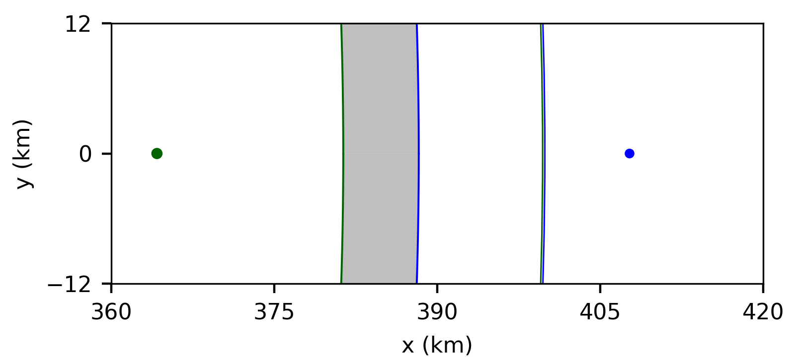
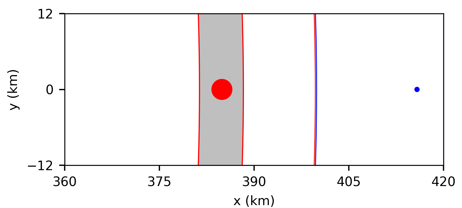
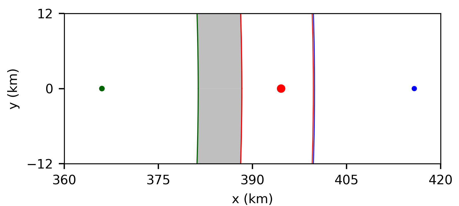
Figure 7: Confinement models for Chariklo rings. The top panel corresponds to a model in which the inner/outer edges of both rings are held by the same inner/outer shepherd satellite. In the middle panel, a satellite confines C1R in its horseshoe region and holds C2R inner edge, while a shepherd satellite confines C2R outer edge. The bottom panel corresponds to a model with the innermost and outermost edges of the system are confined by a pair of satellites and the gap maintained by a third satellite. Satellites are given by dots with colours matching those of the edges they confine, while the grey regions represent the width of the rings. For location and physical radius of the satellites, refer to Table 3.

Figure 7a shows an envisioned confinement model for the rings, in which the same inner satellite confines the inner edges of both rings, and an outer one confines the outer edges. To obtain the radius and position of the shepherd satellites, we followed an approach similar to Murray & Thompson (1990) and calculated the location of the $m+1$:$m$ ERs associated with a hypothetical satellite, checking if any matches the edges of the rings. For the inner edges, we look for resonances in the range $1\leq m\leq 30$ and varied the satellite position from $a_{s}=160$ km until the C1R inner edge, keeping a semi-major axis interval of 100 m. For the outer edges, we assumed the range of $-30\leq m\leq-1$, with the satellite position varying by steps of 100 m from the C2R outer edge until $a_{s}=500$ km.

The resonance location is obtained numerically following the prescription given in Sicardy (2020) for an ellipsoidal object, with the resonance condition given by

$$m(\Omega_{k,s}-\Omega_{k})=\kappa$$ (22)

where $\Omega_{k,s}$ is the angular frequency of the satellite and $\kappa$ is the radial frequency at the edge. After identifying a resonance between satellite and edge, we calculate the satellite’s mass using equation 19. For simplicity, we will assume the satellite with the same bulk density as the ring particles, that is, a satellite made of ice ($\rho=10^{3}$ kg/m³). For denser materials (e.g. silicates) without porosity, satellites smaller in radius are able to confine the ring, which means that our results correspond to an upper limit on the size of a possible shepherd satellite.

Table 3 shows some possible locations for the shepherd satellites, along with the ER that confines the edge, the minimum satellite radius, and which edge is confined. Due to the proximity between first and second-order resonances for larger values of $m$, there is a possibility that $m+2$:$m$ ERs with the shepherd satellites reside within the ring. These resonances are also responsible for angular momentum exchanges and, if they are inside a ring, they act to excite the particles. Seen that, we present in Table 3 only the cases where the satellite generates a second-order resonance residing within C1R. In slanted style, we emphasise the hypothetical satellites that could confine two edges simultaneously due to discrete ERs, corresponding to cases that could produce the confinement envisioned in this subsection. In Figure 7a, we present only one of the possible satellite configurations capable of confining the rings: the inner edges of C1R and C2R are supported by a $390$ m-sized satellite due to a 16:15 and 8:7 ERs, respectively. The outer edges are confined by a satellite of $320$ m of radius due to 12:13 (C1R) and 25:26 (C2R) ERs.

Cordelia and Ophelia straddle the $\epsilon$ ring, but also confine the $\delta$ (23:22 ER) and $\gamma$ (6:5 ER) rings, respectively (French et al., 1991; Nicholson et al., 2018). It is interesting to see that a similar mechanism can occur for Chariklo rings. Based on the numerical simulations of Hänninen & Salo (1994, 1995), Goldreich et al. (1995) show that extremely narrow rings can be held by a single satellite in eccentric resonance, which we can envision to be the mechanism confining C2R. In this case, we would need only one satellite simultaneously in ER with one edge of each ring.

This single-sided shepherding is the mechanism that confine some ringlets of the C ring (Lewis et al., 2011) and occurs when the satellite torque is sufficient to reverse the angular momentum integrated over the ring streamlines (see Borderies et al., 1989). Sickafoose & Lewis (2019) explored the single-sided shepherding for Chariklo rings and obtained encouraging results indicating that a single satellite might model both rings.

Rappaport (1998) show that the torque originating from a dense narrow ring can confine the edge of another ring, which can lead us to speculate more complex confinement scenarios, such as satellites confining C2R and the inner edge C1R, while C2R holds the outer edge of C1R. However, such scenarios are only possible under specific conditions, and the confinement by a pair of satellites is a more credible mechanism.

The confinement by only one pair of shepherd satellites has the facility to spare a satellite in comparison to the classic model discussed in Section 5.3.3. However, it leaves the system without a mechanism for removing material from the gap. The absence of material between the rings can be explained without additional effects only if the two rings formed independently. Now, if they formed in a single event, an additional mechanism must have acted in the system removing material and helping to define the sharp edges of both rings.

5.3.2 Confinement by a co-orbital satellite

In this section, we rescued the works of Dermott et al. (1979, 1980) for narrow rings and proposed a model where C1R would be confined to the horseshoe region of a satellite. The interesting point is that such a model has the convenience of explaining the eccentric shape of C1R since the ring will have the same eccentricity as the satellite (Dermott et al., 1979). From equation 15, we obtain that C1R is confined by a satellite with 2 km of radius, shown in Figure 7b by the red dot. An external satellite is required to hold C2R outer edge. In the figure, the blue dot corresponds to a satellite holding C2R at 14:15 ER (Table 3).

A satellite with 2 km of radius would be responsible for generating a chaotic region of half-width of $15$ km (eq. 16). Given that, the gap has an extension of $13.9$ km, therefore the C2R would be wholly embedded in the chaotic region, which could be an argument to invalidate this model. However, we remind the reader that the recipe to get the chaotic region was developed assuming objects such as mass point. When considering Chariklo as a non-spherical body and the gravitational effects of other nearby satellites, the extension of the chaotic region may change, perhaps allowing a regular motion in the C2R region. In this line of thought, the C2R would reside at the edge of the chaotic region, and therefore a single satellite would confine C1R and produce the gap.

5.3.3 Classic confinement model

An already classic confinement model for Chariklo rings was proposed in BR14, in which C1R inner edge and C2R outer edge would be confined by an ER with an inner and outer shepherd satellites, respectively. Additionally, a third satellite would be responsible for the gap between the structures, in analogy, for example, to the satellite Daphnis, responsible for maintaining the Keeler Gap in the A ring of Saturn (Weiss et al., 2009).

We qualitatively explore this model using the most recent observational data provided in M21, first estimating the mass needed for a satellite to hold the gap. Assuming an object made of ice and located at $a_{s}=392.9$ km, we obtain from equation 21 a radius of $\sim 150$ m.

Equation 21 gives the width of the gap opened by a satellite in a ring implying that C1R and C2R in the past were a single ring that were separated by this satellite. This is compatible, for example, with a scenario in which the disruption of an object originated a ring of material with the satellite being the largest fragment, or with a scenario whose satellite was formed in situ from material from an ancient ring.

As previously shown in Section 4, the 1:3 spin-orbit resonance with Chariklo is located between the two rings for large values of eccentricity. A satellite trapped in this resonance can open a gap between the rings and prevent them from spreading. If in 1:3 spin-orbit resonance, a satellite in the gap will have a minimum eccentricity of $0.02$ – and maximum eccentricity of $0.29$ (Figure 6) – and this, can contribute to C1R eccentricity (Colwell et al., 2009). Therefore, it is possible that the inner edge of C1R and the outer edge of C2R are being held by shepherd satellites, while a satellite in 1:3 spin-orbit resonance with Chariklo maintains the gap between the rings.

An example of a system in this confinement model is shown in Figure 7c. The innermost satellite (green dot) has $320$ m of radius and confines C1R inner edge (solid green line) due to a 18:17 ER. The outer edge of C2R (solid blue line) in the figure is confined by 14:15 ER with a $290$ m-sized satellite (blue dot), while the C1R outer edge and C2R inner edge (red solid lines) result from the gap caused by a $500$ m-sized satellite (red dot).

The fact that the satellites involved in the confinement have radii less than one kilometre makes the classic model quite attractive, since a set of reasonable origins can be imagined for these satellites. Some examples are capture or disruption of an ancient satellite. The detection by occultation of angularly tiny objects near a ring is highly unlikely (Sicardy et al., 2015), explaining why these objects were not detected if they actually exist. Finally, the possibility of C1R and C2R having been a single entity in the past is a very appealing point for formation models.

A pragmatic analysis of the models presented here requires more extensive investigations, as it is still unknown how the physical processes discussed here are affected by the ellipsoidal shape of Chariklo. Our intention in this section is not to explain the dynamics of the Chariklo rings but only present some discussions that can be useful for future works on rings around non-axisymmetric bodies.

6 Discussion

The discovery of Chariklo’s rings (C1R and C2R) brought new insight into planetary ring dynamics. A set of particles orbiting around small objects (compared to the giant planets) asymmetrically shaped is a new topic to be explored. According to the most recent data (M21) the mean width of C1R is about 7 km (a narrow ring), while its eccentricity is between 0.005 to 0.022. C2R is an even narrower ring, 120 m. Our work aims to bring new insights into the dynamics of this unusual ring system. Through a set of numerical simulations and an analysis of periodic and quasi-periodic orbits, we derived the following main results. The width of the unstable region, due to the irregular shape of Chariklo, is smaller when compared with the results presented in Sicardy et al. (2019). This difference is caused by the new parameters derived for the shape of Chariklo.

The presence of gravitational interaction between the ring particles will cause larger damping due to collisions, making the disk more circular (decreasing in the eccentricity). Although it probably will not change the size of the unstable region. Analysis of massive bodies with self-gravity is under investigation.

Through a detailed analysis of a sample of Poincaré surface of sections we derived the size and location of the stable region in a diagram $a_{eq}$ versus $e_{eq}$. For a given ring width (9 km for C1R), we computed values of $e$ and $a$ that a particle located on the inner or outer edge of the ring could assume. This places the inner ring (C1R) in the stable region if its eccentricity is larger than $6\times 10^{-4}$, which corroborates with the recent results. However, C2R is located outside the stable region. To be in the stable region, C2R needs to have a larger eccentricity value, and consequently a larger width. Therefore, the last data regarding the width of C2R needs to be revisited.

Three confinement mechanisms are discussed in light of the theory of the known narrow planetary rings of the giant planets. The classical confinement model seems to be the most suitable. This model requires three small moonlets to confine the edges of the rings. Two small moonlets, interior to the inner edge of C1R and exterior to the outer edge of C2R, prevent the spreading in the rings through ERs (mean motion resonance). The gap between the rings would be opened by a third satellite located in the 1:3 spin-orbit resonance.

Due to the small satellites sizes required by the confinement models, it is possible to form the shepherd satellites in situ from an old ring or directly by disruption of an older object, which would also give rise to a ring of material. Both scenarios share similarities of requiring an ancient ring from which C1R and C2R were carved due to satellites gravitational effects.

The eccentric and narrow shape of Chariklo rings seems to indicate that the system around the Centaur is more complex than we know, probably hosting shepherd satellites.

During the review of this paper two rings (Q1R and Q2R) were discovered by Morgado et al. (2023) and Pereira et al. (2023) around the trans-Neptunian object (5000) Quaoar located at 43.3 au. Besides the rings, a satellite, Weywot, orbits Quaoar at about 24 radii of the central body. Both rings are well located interior to the orbit of Weywot. Q1R, at 7.4 radii from Quaoar, is a dense and irregular ring, resembling the clumpy F ring of Saturn (Morgado et al., 2023). The intriguing fact regarding this system is that Quaoar’s rings are outside to its Roche limit, where dense rings are expected to accrete into satellites. Morgado et al. (2023) claimed that collisions may keep the ring even outside the Roche limit.

More data on rings around Centaurs are needed to assess whether Chariklo is a rule or an exception among this class of objects, what will allow us to trace the plausibility of the mechanisms discussed. In fact, new data regarding different ring systems around different primary bodies will help us to unravel the dynamics involved in each system.