Unified theory of classical and quantum signal sensing with a qubit

Abstract

Quantum sensing protocols typically uses a quantum sensor to sense classical signals with the standard Ramsey inteferometry measurements. The classical signals are often real numbers determining the sensor Hamiltonian. However, for a senor embedded in a quantum environment, the signal to detect may be a quantum operator on a target quantum system. There is still no systematic method to detect such a quantum signal. Here we provide a general framework to sense static quantum signals with a qubit sensor by the Ramsey interferometry measurements, with the static classical signal sensing incorporated as a special case. This framework is based on a novel approach to simultaneously estimating the eigenvalues of the quantum signal operator with sequential projective measurements of the sensor, which can extract useful information about the target quantum system. The scheme can also be extended to sense ac quantum signals with dynamical decoupling control of the sensor. As an example, we show that a qubit sensor can simultaneously detect the individual coupling strengths with multiple target qubits in a spin-star model.

Quantum sensing concerns the task of measuring physical quantities with a quantum sensor Degen2017 ; Giovannetti2004 ; Giovannetti2011 ; Pirandola2018 . Quantum properties, such as quantum coherence or entanglement, can make the quantum sensor have better measurement sensitivity or precision than classical sensors Bollinger1996 ; Giovannetti2006 ; Balasubramanian2008 ; Maze2008 ; Rondin2014 ; Barry2020 . Quantum sensing protocols often follow the generic steps including sensor initialization, interaction with the signal, sensor measurement and signal estimation. A canonical sensing protocol is the Ramsey interferometry measurement (RIM) Ramsey1950 ; Lee2002 ; Taylor2008 ; Liu2019 , where a classical signal acts as a static parameter in the qubit sensor Hamiltonian [Eq. (1)] (this signal is classical in the sense that it is only a real number). With the RIM sequence, the classical signal influences the probabilities of the measurement results in a single RIM. The measurement outcomes of different RIMs are assumed to be independent and identically distributed. So by repeating the RIMs sequentially and averaging over the measurement results, the classical signal can be accurately estimated within standard quantum limit. Various other schemes based on sequential or continuous measurements have been proposed to estimate unknown parameters in open quantum systems Mabuchi1996 ; Gambetta2001 ; Catana2012 ; Guta2011 ; Gammelmark2013 ; Gammelmark2014 ; Horssen2015 ; Kiilerich2015 ; Burgarth2015 ; Demkowicz2017 ; Zhou2018 .

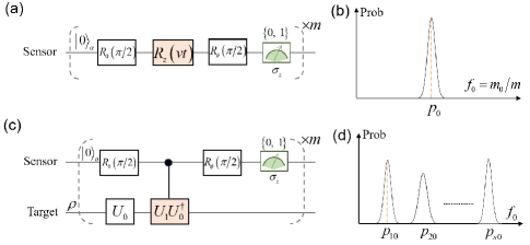
Figure 1: Quantum circuits and measurement statistics of classical and quantum signal sensing with sequential RIMs. (a) Quantum circuit for sensing a classical signal $v$ [$R_{z}(vt)=e^{-ivt\sigma_{z}}$] with a qubit sensor. Each measurement has two outcomes $\{0,1\}$. The probability to obtain outcome 0 is $p_{0}=[1-\cos(2vt+\phi)]/2$, and the number of outcome 0 in $m$ measurements is denoted as $m_{0}$. (b) The probability of the frequency $f_{0}=m_{0}/m$ of outcome 0 for classical signal sensing, which obeys a binomial distribution around $p_{0}$. (c) Quantum circuit for sensing a quantum signal $V$ ($U_{0}=e^{-iVt}$ and $U_{1}=U_{0}^{\dagger}$) with the set of eigenvalues $\{v_{k}\}_{k=1}^{s}$. (d) The probability distribution of $f_{0}$ for quantum signal sensing, which can display multiple binomial distributions around $\{p_{10},\cdots,p_{s0}\}$ with $p_{k0}=[1-\cos(2v_{k}t+\phi)]/2$.

In practice, a quantum sensor is embedded in a quantum environment, with the target system as part of this quantum environment, such as a nitrogen-vacancy (NV) electron spin to detect some nuclear spins in a spin bath Zhao2011 ; Zhao2012 ; Kolkowitz2012 ; Taminiau2012 ; Shi2014 ; Abobeih2019 . So generally the signal to detect should be a quantum signal, that is, a Hermitian operator on the target system [Eq. (6)]. The quantum signal operator can be either static or time-varying. For a time-varying quantum signal operator, its influence on the sensor can sometimes be approximated by a classical stochastic noise Abobeih2019 ; Cywinski2008 ; Witzel2014 ; Ma2015 , but exploiting the quantum nature of the signal operator enables the detection of high-order quantum correlations and quantum non-linear spectroscopy Wang2019 ; Wu2022 ; Wang2021 ; Meinel2022 ; Shen2023 . A more basic problem is to fully sense a static quantum signal operator (such as its eigenvalues), which corresponds exactly to the static classical signal sensing with RIMs. This poses several interesting questions: can we design a scheme to sense such static quantum signals? What information about the signals can we detect? What is the relationship between the classical and quantum signal sensing in this sense?

In this paper, we answer these questions by developing a unified framework to sense both classical and quantum signals with a qubit senor. The important finding is that the sequential RIM protocol generally works for sensing the eigenvalues of static quantum signals, with the static classical signal sensing as a special case. But in contrast to classical signal sensing, the measurement statistics of sequential RIMs are not independent and identically distributed. Each RIM of the sensor induces a quantum channel (or generalized quantum measurement) on the target quantum system. For sequential RIMs of the sensor, the target system is gradually steered to the fixed points of the quantum channel, corresponding to the states in different eigenspaces of quantum signal operator. Conversely, the gradual state change of the target system will influence the sensor measurement statistics. Surprisingly, the sensor measurement statistics can display multiple binomial distributions [Eq. (19)], with each distribution concentrating around some value determined by the eigenvalues of the quantum signal operator. When the target system initially start from an eigenstate of the quantum signal Hamiltonian, the measurement statistics shows a single binomial distribution and is thus equivalent to the case of classical signal sensing [Eq. (5)]. With dynamical decoupling (DD) control of the sensor, the sequential RIM scheme can also detect ac quantum signals. As an example, we show sequential RIMs can be utilized to estimate the individual coupling strengths in a spin-star model.

RIMs for sensing classical signals. We start by reviewing the standard RIM for sensing a classical signal [Fig. 1(a)]. A sensor qubit is directly coupled to a static classical signal with a sensing Hamiltonian

$$H_{c}=v\sigma_{z}=v(|0\rangle_{a}\langle 0|-|1\rangle_{a}\langle 1|),$$ (1)

where $v$ is the classical signal amplitude and $\sigma_{i}$ is the Pauli-$i$ operator of the ancilla qubit ($i=x,y,z$). Hereafter we denote the sensor rotation along the axis in equatorial plane as $R_{\phi}(\theta)=e^{-i(\cos\phi\sigma_{x}+\sin\phi\sigma_{y})\theta/2}$ with $\phi$ denoting the rotation axis and $\theta$ being the rotation angle. In a single RIM sequence, the qubit initialized to state $|0\rangle_{a}$, first undergoes a rotation $R_{\phi_{1}}(\pi/2)$, then evolves with the sensor Hamiltonian $H$ for time $t$, undergoes another rotation $R_{\phi_{2}}(\pi/2)$ with the resultant state

$$R_{\phi_{2}}(\pi/2)R_{z}(vt)R_{\phi_{1}}(\pi/2)|0\rangle_{a}$$

$$= \frac{1}{2}\left[{\begin{array}[]{*{20}{c}}{{e^{-ivt}-e^{i(\Delta\phi+vt)}}}\\ {-ie^{i\phi_{2}}\left({e^{-ivt}+e^{i(\Delta\phi+vt)}}\right)}\end{array}}\right]_{a},$$ (4)

where $R_{z}(vt)=e^{-ivt\sigma_{z}}$, and $\Delta\phi=\phi_{1}-\phi_{2}$. Finally a projective measurement (PM) is performed on the sensor with the readout basis $\{|0\rangle,|1\rangle\}$. The probability distribution for the outcomes $\{0,1\}$ is $F^{\prime}=(p_{0},p_{1})$ with $p_{0}=[1-\cos(2vt+\Delta\phi)]/2$ and $p_{1}=1-p_{0}$.

The RIM are repeated $m$ times, and the frequencies of measurement outcomes are recorded as $F=(f_{0},f_{1})$. Then $F$ obeys a binomial distribution Bengtsson2017

$$p_{c}(F)=\frac{m!}{(mf_{0})!(mf_{1})!}p_{0}^{mf_{0}}p_{1}^{mf_{1}}\approx e^{-mS(F\|F^{\prime})},$$ (5)

where $S(F\|F^{\prime})=\sum_{i=0,1}f_{i}\ln(f_{i}/p_{i})$ is the relative entropy between $F$ and $F^{\prime}$. For large $m$, the above probability distribution is concentrated around $F^{\prime}$ as a Gaussian distribution since $S(F\|F^{\prime})\approx\sum_{i=0,1}(f_{i}-p_{i})^{2}/(2p_{i})=(f_{0}-p_{0})^{2}/(2p_{0}p_{1})$ [Fig. 1(b)]. Therefore, $F^{\prime}$ can be approximated by the most probable $F$ with the standard deviation $\sqrt{p_{0}p_{1}/m}$, and the classical signal $v$ can be inferred from $F$ with a known free evolution time $t$.

RIMs for sensing quantum signals. We provide a basic model to sense a static quantum signal [Fig. 1(c)]. Suppose the sensor is coupled to a $d$-dimensional target quantum system with the coupling Hamiltonian Degen2017

$$H_{q}=\sigma_{z}\otimes V=\sum_{k=1}^{s}v_{k}\sigma_{z}\otimes P_{k},$$ (6)

where $V$ is a Hermitian operator on the target system, $\{v_{k}\}_{k=1}^{s}$ is the set of eigenvalues of $V$, and $\{P_{k}\}_{k=1}^{s}$ is the set of projection operators satisfying $\sum_{k=1}^{s}P_{k}=\mathbb{I}$ with $\mathbb{I}$ being the identity operator on the target system. Our objective is to characterize the quantum signal $V$ by estimating the set of eigenvalues $\{v_{k}\}_{k=1}^{s}$.

With the target system prepared in an eigenstate with eigenvalue $v_{k}$, the quantum signal Hamiltonian [Eq. (6)] can be replaced by a classical one [Eq. (1)]. So we can estimate $v_{k}$ by RIMs, with the same steps as those in sensing classical signals. This is quite analogous to the quantum phase estimation algorithm Nielsen2010 ; Cleve1998 , which is also designed to estimate eigenvalues of a unitary.

For the target system in an arbitrary state $\rho$, a single RIM on the sensor induces a quantum channel Wolf2010 ; Caruso2014 ; Watrous2018 on the target system, which can be represented in the Stinespring representation as Stine1955

$$\Phi(\rho)={\rm Tr}_{a}[U(t)(\rho_{a}\otimes\rho)U^{\dagger}(t)],$$ (7)

where $U(t)=e^{-iH_{q}t}=|0\rangle_{a}\langle 0|\otimes U_{0}+|1\rangle_{a}\langle 1|\otimes U_{1}$ with $U_{0}=\sum_{k=1}^{s}e^{-iv_{k}t}P_{k}$ and $U_{1}=U_{0}^{\dagger}$, $\rho_{a}=|\psi\rangle_{a}\langle\psi|$ with $|\psi\rangle_{a}=R_{\phi_{1}}(\pi/2)|0\rangle_{a}$, and ${\rm Tr}_{a}$ denotes the partial trace over the sensor. This quantum channel can also be transformed to the Kraus representation as Kraus1983

$$\Phi(\rho)=M_{0}\rho M_{0}^{\dagger}+M_{1}\rho M_{1}^{\dagger},$$ (8)

with the Kraus operators $M_{0}=(U_{0}-e^{i\Delta\phi}U_{1})/2$ and $M_{1}=(U_{0}+e^{i\Delta\phi}U_{1})/2$. Note that $\Phi$ is independent of the second rotation $R_{\phi_{2}}(\pi/2)$, while $M_{0}$ and $M_{1}$ depend on the phase difference $\Delta\phi$ between $R_{\phi_{1}}(\pi/2)$ and $R_{\phi_{2}}(\pi/2)$. The probability to obtain result 0 is $p_{0}={\rm Tr}(M_{0}\rho M_{0}^{\dagger})=[1-\sum_{k=1}^{s}{\rm Tr}(P_{k}\rho)\cos(2v_{k}t+\Delta\phi)]/2$.

If the probability distributions of each RIM are assumed to be independent and identical, we can still repeat the RIMs, estimate $\{v_{k}\}_{k=1}^{s}$ by recording $p_{0}(t)$ as a function of $t$ and then perform Fourier analysis to find the frequency components. This is the method to perform spectral analysis of a unitary in the model of deterministic quantum computation with one quantum bit (DQC1) Knill1998 ; Datta2005 ; Datta2008 ; Cable2016 . However, this method neglects the backaction of sensor measurements on the target system state in the sequential RIM scheme. Actually the target system undergoes different state jumps with different measurement outcomes of the sensor in a single RIM, which will influence the statistics of the next RIM. Therefore, the statistics of sequential RIMs will show some non-classical features. The main finding in this paper is that such non-classical features of measurement statistics can be utilized to efficiently estimate $\{v_{k}\}_{k=1}^{s}$. Below we exactly solve the backaction and measurement statistics of sequential RIMs for sensing quantum signals.

Backaction of sequential RIMs. To analyse the backaction of sequential RIMs on the target system, it is illuminating to study the behaviors of sequential applications of the quantum channel $\Phi$. Previous works have studied the asymptotic behaviors of sequential quantum channels Albert2019 ; Burgarth2013 ; Novotny2018 ; Blume2010 . Our recent work shows that sequential quantum channels with normal and commuting Kraus operators can simulate a PM in the asymptotic limit Ma2023 . Our derivations below make use of this recent theoretical finding.

First we introduce the natural representation of a quantum channel on the Hilbert-Schmidt (HS) space of the target system Bengtsson2017 ; Watrous2018 . The space of operators on the Hilbert space of the target system form a linear vector space called the HS space, as can be seen by the matrix reshaping, $X=\sum_{i,j=1}^{d}x_{ij}|i\rangle\langle j|\leftrightarrow|X\rangle\rangle=\sum_{i,j=1}^{d}x_{ij}|ij\rangle\rangle$. The inner product in the HS space is defined as $\langle\langle Y|X\rangle\rangle={\rm Tr}(Y^{\dagger}X)$. Then the superoperator $X(\cdot)Y$ on the Hilbert space is equivalent to a linear operator $X\otimes Y^{T}$ on the HS space, so the channel $\Phi$ can be naturally represented as $\hat{\Phi}=\hat{\mathcal{M}}_{0}+\hat{\mathcal{M}}_{1}$ with $\hat{\mathcal{M}}_{\alpha}=M_{\alpha}\otimes M_{\alpha}^{*}$ with $\alpha\in\{0,1\}$ (note that we add hats for operators acting on the HS space). With the HS space, the probability to get the $\alpha$th outcome is $\langle\langle\mathbb{I}|\hat{\mathcal{M}}_{\alpha}|\rho\rangle\rangle={\rm Tr}(M_{\alpha}\rho M_{\alpha}^{\dagger})$.

The channel $\hat{\Phi}$ can be recast into a neat form if we rewrite the Kraus operators as Ma2023

$$\left[{\begin{array}[]{*{20}{c}}{{M_{0}}}\\ {{M_{1}}}\end{array}}\right]=\left[{\begin{array}[]{*{20}{c}}{{\bm{\lambda}_{1}}}&\cdots&{{\bm{\lambda}_{s}}}\end{array}}\right]\left[{\begin{array}[]{*{20}{c}}{{P_{1}}}\\ \vdots\\ {{P_{s}}}\end{array}}\right],$$ (15)

where $\bm{\lambda}_{k}=[e^{-iv_{k}t}-e^{i(\Delta\phi+v_{k}t)},-ie^{i\phi_{2}}(e^{-iv_{k}t}+e^{i(\Delta\phi+v_{k}t)})]^{T}/2$ is a unit column vector satisfying $\langle\bm{\lambda}_{k},\bm{\lambda}_{k}\rangle=1$, with $\langle\cdot,\cdot\rangle$ denoting the Euclidean inner product in the complex vector space. Then $\{\bm{\lambda}_{k}\}_{k=1}^{s}$ is a set of such unit vectors. Intriguingly, $\bm{\lambda}_{k}$ is similar to the sensor wavefunction in Eq. (Unified theory of classical and quantum signal sensing with a qubit). Then $\hat{\Phi}$ becomes a diagonal operator in the HS space as

$$\hat{\Phi}=\sum_{k,l=1}^{s}\langle\bm{\lambda}_{l},\bm{\lambda}_{k}\rangle P_{k}\otimes P_{l},$$ (16)

with the eigenvalues $\{\langle\bm{\lambda}_{l},\bm{\lambda}_{k}\rangle\}_{k,l=1}^{s}$. Since $|\langle\bm{\lambda}_{l},\bm{\lambda}_{k}\rangle|\leq\langle\bm{\lambda}_{l},\bm{\lambda}_{l}\rangle\langle\bm{\lambda}_{k},\bm{\lambda}_{k}\rangle=1$ due to the Cauthy-Schwarz inequality Garcia2017 , all the eigenvalues of $\hat{\Phi}$ lie within the unit disk of the complex plane. The eigenvectors of $\hat{\Phi}$ with eigenvalue 1 are called fixed points Arias2002 , and and those with eigenvalues $e^{i\varphi}$ with $\varphi\neq 0$ are rotating points Albert2019 . The HS subspace spanned by the fixed points and rotating points are called asymptotic subspace (also known as peripheral or attractor subspace). If any two unit vectors in $\{\bm{\lambda}_{k}\}_{k=1}^{s}$ are not parallel, then the asymptotic subspace contains only the fixed points, which are all eigenstates of $V$. With sequential applications of $\hat{\Phi}$, the projections to the asymptotic subspace remain unchanged, while the projections to the other eigenspaces gradually vanish Albert2019 ; Burgarth2013 ; Novotny2018 ; Blume2010 . So for large $m$, $\hat{\Phi}^{m}\approx\sum_{k=1}^{s}\hat{\mathcal{P}}_{k}$ approximates a PM on the target system Ma2023 ; Ma2018 ; Wang2023 ; Liu2017 ; Rao2019 ; Dasari2022 , with $\hat{\mathcal{P}}_{k}=P_{k}\otimes P_{k}$ corresponding to the projection superoperator $P_{k}(\cdot)P_{k}$.

Measurement statistics of sequential RIMs. The normal and commuting Kraus operators [Eq. (15)] also allow an exact solution of the measurement statistics for sequential RIMs. Since $[\hat{\mathcal{M}}_{0},\hat{\mathcal{M}}_{1}]=0$, we can expand $\hat{\Phi}^{m}$ according to the binomial theorem, $\hat{\Phi}^{m}=\sum_{F}\hat{\Phi}^{m}(F)$ with

$$\hat{\Phi}^{m}(F)=\frac{m!}{(mf_{0})!(mf_{1})!}\hat{\mathcal{M}}_{0}^{mf_{0}}\hat{\mathcal{M}}_{1}^{mf_{1}}.$$ (17)

With a reasoning similar to that in Eq. (5), we get

$$\hat{\Phi}^{m}(F)\approx\sum_{k=1}^{s}e^{-mS(F\|F_{k})}\hat{\mathcal{P}}_{k},$$ (18)

where $F_{k}=(p_{k0},p_{k1})$ with $p_{k0}=[1-\cos(2v_{k}t+\Delta\phi)]/2$. If $\bm{\lambda}_{k}$ is regarded as a wavefunction [Eq. (Unified theory of classical and quantum signal sensing with a qubit)], $F_{k}$ is just the probability amplitude distribution. Then the probability distribution for the measurement result $F$ is

$$p_{q}(F)=\langle\langle\mathbb{I}|\hat{\Phi}^{m}(F)|\rho\rangle\rangle\approx\sum_{k=1}^{s}e^{-mS(F\|F_{k})}{\rm Tr}(P_{k}\rho),$$ (19)

where we have used $\langle\langle\mathbb{I}|\hat{\mathcal{P}}_{k}|\rho\rangle\rangle={\rm Tr}(P_{k}\rho)$.

Eq. (19) represents a summation of at most $s$ different binomial distributions around $F_{1},\cdots,F_{s}$ [Fig. 1(d)]. The weight of the $k$th binomial distribution is ${\rm Tr}(P_{k}\rho)$, that is, the projection of the initial target system $\rho$ on the $k$th eigenspace of the quantum signal operator $V$. So if the target system starts from an eigenstate of $V$, the single binomial distribution [Eq. (5)] in classical signal sensing is recovered. Interestingly, the initial maximally mixed state of the target system is desirable for quantum sensing, since then all the binomial distributions can appear, and integration of the measurement results for $k$th distribution also heralds a selective PM $\hat{\mathcal{P}}_{k}$ on the target system Ma2023 . Any two binomial distributions around $F_{k}$ and $F_{l}$ can are well separated if the distance between $F_{k}$ and $F_{l}$ is larger than the sum of the respective half widths of the distribution. This requires $m>2|\ln\eta|(\sqrt{p_{k0}p_{k1}}+\sqrt{p_{l0}p_{l1}})/|p_{k0}-p_{l0}|$, where $\eta$ is the ratio of the minimum hight to the maximum hight within the distribution width. Then for large $m$, all the binomial distributions can be well distinguished and therefore the eigenvalue set $\{v_{k}\}_{k=1}^{s}$ of the quantum signal operator $V$ can be accurately estimated within the standard quantum limit.

Extension to ac quantum signal sensing. So far we have assumed that the quantum signal is static and determinant, but the RIM scheme can also sense a time-dependent quantum signal operator. First recall that for a classical time-dependent signal $v(t)$, the RIM scheme can detect the integration of such a signal $\int_{0}^{t}v(t^{\prime})dt^{\prime}$. For quantum signal sensing, it is crucial to note that the RIM scheme actually detect the eigenvalues of the unitary operator $U_{0}^{\dagger}U_{1}$ with the condition $[U_{0},U_{1}]=0$. For a time-dependent quantum signal operator $V(t)$, $U_{0}=\mathcal{T}e^{-i\int_{0}^{t}V(t^{\prime})dt^{\prime}}$ and $U_{1}=\mathcal{T}e^{i\int_{0}^{t}V(t^{\prime})dt^{\prime}}$ with $\mathcal{T}$ being the time-ordering operator. If $U_{0}$ and $U_{1}$ can be well approximated by the first-order Magnus expansion, i.e., $U_{0}\approx e^{-i\int_{0}^{t}V(t^{\prime})dt^{\prime}}\approx U_{1}^{\dagger}$, then $[U_{0},U_{1}]=0$ and the RIM scheme can approximately detect the eigenvalues of the operator $\int_{0}^{t}V(t^{\prime})dt^{\prime}$.

In particular, the RIM scheme can perform ac quantum signal sensing with DD control of the sensor. The $N$-pulse DD control of the sensor consists of a sequence of $\pi$ flips at times $\{t_{1},t_{2},\cdots,t_{N}\}$ for the sensor evolution from 0 to $t$. If the target system has a free Hamiltonian and the sensor is under DD control within each RIM cycle, the Hamiltonian becomes

$$H^{\prime}_{q}=f(t)\sigma_{z}\otimes V+H_{0},$$ (20)

where $H_{0}=\sum_{i=1}^{d}\varepsilon_{i}|i\rangle\langle i|$ is the free Hamiltonian, $V=\sum_{i,j=1}^{d}V_{ij}|i\rangle\langle j|=\sum_{\omega}V(\omega)$ with $V(\omega)=\sum_{\varepsilon_{i}-\varepsilon_{j}=\omega}V_{ij}|i\rangle\langle j|$, and $f(t)$ is the DD modulation function jumping between $+1$ and $-1$ every time the sensor is flipped by a DD pulse. If $[V,H_{0}]=0$, the quantum signal is still static and thus the above RIM scheme works. However, if $[V,H_{0}]\neq 0$, the quantum signal becomes $V(t)=e^{iH_{0}t}Ve^{-iH_{0}t}=\sum_{\omega}e^{i\omega t}V(\omega)$ in the interaction picture, which can be termed as an ac quantum signal. Then DD control of the sensor can select some specific component $V(\omega)$ and filter out the other parts in $V$, if $f(t)$ is periodic and its frequency matches $\omega$. Then $U_{0}^{\dagger}U_{1}\approx{\rm exp}\{2i[F(\omega,t)V(\omega)+F^{*}(\omega,t)V^{\dagger}(\omega)])\}$ with $F(\omega,t)=\int_{0}^{t}f(t^{\prime})e^{i\omega t}dt^{\prime}$, whose eigenvalues can be estimated with sequential RIM sequences.

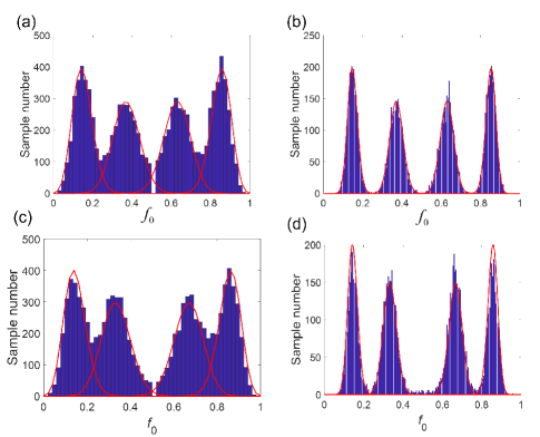
Figure 2: Monte Carlo simulation of quantum signal sensing in a spin-star model. (a,b) For the model in Eq. (21) with $\omega\neq 0$, the histogram of the number of samples as a function of the frequency $f_{0}$ for different repetition times in sequential RIMs: (a) $m$ = 50, (b) $m$ = 200. The parameters are $A_{1}t=0.13$ rad, $A_{2}t=0.26$ rad. (c,d) is similar to (a,b) but corresponds to the model in Eq. (21) with $\omega/A_{1}=2\omega/A_{2}=10$, $\mathbf{n}_{1}=(0.50,0.50,0.71)$, $\mathbf{n}_{1}=(0.10,0.10,0.99)$ and the CPMG pulse number $N=4$. The red solid lines represent the exact probability distribution in Eq. (19), and the initial state of the target qubits are an equal superposition of all the four eigenstates of the quantum signal operator. All the Monte Carlo simulations contain $10^{4}$ samples with $\phi=\pi/2$.

Example: quantum signal sensing in a spin-star model. As an example, we consider a spin-star model with the Hamiltonian

$$H_{\rm star}=\sigma_{z}\otimes\sum_{j=1}^{J}\frac{A_{j}}{4}(\bm{\sigma}_{j}\cdot\mathbf{n}_{j})+\frac{\omega}{2}\sum_{j=1}^{J}\sigma_{j}^{z},$$ (21)

where $\bm{\sigma}_{j}=(\sigma_{j}^{x},\sigma_{j}^{y},\sigma_{j}^{z})$is the Pauli vector for the $j$th target spin and $\mathbf{n}_{j}=(n_{j}^{x},n_{j}^{y},n_{j}^{z})$ is a unit vector. Here the first term denotes the inhomogeneous coupling between the sensor and $N$ target spins, and the second term is an homogeneous Zeeman term of the target spins induced by an external magnetic field.

We consider two cases of this model for quantum signal sensing: (i) Without the Zeeman term ($\omega=0$), the quantum signal is a static operator $V=\sum_{j=1}^{J}A_{j}(\bm{\sigma}_{j}\cdot\mathbf{n}_{j})$ with eigenvalues $v_{k}=\sum_{j=1}^{J}\xi_{jk}A_{j}/4$ for $\xi_{jk}\in\{1,-1\}$, so we can fully determine $\{v_{k}\}_{k=1}^{2^{J}}$ with sequential RIMs and thus the coupling strengths $\{A_{j}\}_{j=1}^{J}$. (ii) With the Zeeman term ($\omega\neq 0$), we can apply the $N$-pulse Carr-Purcell-Meiboom-Gill (CPMG) control to the sensor with the flip pulses at times $\{t_{l}=(2l-1)\tau\}_{l=1}^{N}$ ($2\tau=t/N$). With the resonant DD condition ($2\tau=\pi/\omega$), $U_{0}^{\dagger}U_{1}\approx\prod_{j=1}^{J}{\rm exp}[iA_{j}^{\perp}N(\cos\kappa_{j}\sigma_{j}^{x}-\sin\kappa_{j}\sigma_{j}^{y})/(2\omega)]$ with $A_{j}^{\perp}=A_{j}[(n_{j}^{x})^{2}+(n_{j}^{y})^{2}]$ and $\kappa_{j}={\rm arg}(F(\omega,t))+{\rm arctan}(A_{j}^{y}/A_{j}^{x})$, so by sequential RIMs we can estimate $\{A_{j}^{\perp}\}$, which are the components of the interaction fields $\{A_{j}\mathbf{n}_{j}\}$ perpendicular to the external magnetic field. With several different directions of the external magnetic field, we can estimate both $\{A_{j}\}$ and $\{\mathbf{n}_{j}\}$ Ma2016 .

For both cases of the spin-star model, we perform Monte Carlo calculations to simulate the measurement statistics of sequential RIMs for two target spins. The results in Fig. 2 show four distinct binomial distributions as the repetition number $m$ of RIMs increases, which correspond to the four different eigenvalues of the quantum signal operators.

Conclusions and outlooks. We develop a unified theoretical framework to sense both classical and quantum signals with sequential RIMs. For quantum signal sensing, the measurement statistics can display multiple distribution peaks, which can be used to precisely estimate the eigenvalues of the quantum signal operator on a target quantum system. The measurement statistics of classical signal sensing can be recovered when the target system starts from an eigenstate of the quantum signal operator. The concept and proposal of quantum signal sensing greatly broaden the scope of quantum sensing concerning mostly about classical signals before. The unified framework also raises further problems to explore, which can be inspired by topics in classical signal sensing. In particular, it will be interesting to consider a more complex sensor (such as a sensor with multiple qubits, a qudit or even a harmonic oscillator) for quantum signal sensing, and explore the role of quantum coherence and entanglement in improving the sensitivity beyond the standard quantum limit.

- (1) C. L. Degen, F. Reinhard, and P. Cappellaro, Quantum Sensing, Rev. Mod. Phys. 89, 035002 (2017).
- (2) V. Giovannetti, S. Lloyd, and L. Maccone, Quantum-Enhanced Measurements: Beating the Standard Quantum Limit, Science 306, 1330 (2004).
- (3) V. Giovannetti, S. Lloyd, and L. MacCone, Advances in Quantum Metrology, Nat. Photonics 5, 222 (2011).
- (4) S. Pirandola, B. R. Bardhan, T. Gehring, C. Weedbrook, and S. Lloyd, Advances in Photonic Quantum Sensing, Nat. Photonics 12, 724 (2018).
- (5) J. J. Bollinger, W. M. Itano, D. J. Wineland, and D. J. Heinzen, Optimal Frequency Measurements with Maximally Correlated States, Phys. Rev. A 54, R4649 (1996).
- (6) V. Giovannetti, S. Lloyd, and L. MacCone, Quantum Metrology, Phys. Rev. Lett. 96, 010401 (2006).
- (7) G. Balasubramanian et al., Nanoscale Imaging Magnetometry with Diamond Spins under Ambient Conditions, Nature 455, 648 (2008).
- (8) [1] J. R. Maze et al., Nanoscale Magnetic Sensing with an Individual Electronic Spin in Diamond, Nature 455, 644 (2008).
- (9) L. Rondin, J.-P. Tetienne, T. Hingant, J.-F. Roch, P. Maletinsky, and V. Jacques, Magnetometry with nitrogenvacancy defects in diamond, Rep. Prog. Phys. 77, 056503 (2014).
- (10) J. F. Barry, J. M. Schloss, E. Bauch, M. J. Turner, C. A. Hart, L. M. Pham, and R. L. Walsworth, Sensitivity optimization for NV-diamond magnetometry, Rev. Mod. Phys. 92, 015004 (2020).
- (11) N. F. Ramsey, A Molecular Beam Resonance Method with Separated Oscillating Fields, Phys. Rev. 78, 695 (1950).
- (12) H. Lee, P. Kok, and J. P. Dowling, A Quantum Rosetta Stone for Interferometry, J. Mod. Opt. 49, 2325 (2002).
- (13) J. M. Taylor, P. Cappellaro, L. Childress, L. Jiang, D. Budker, P. R. Hemmer, A. Yacoby, R. Walsworth, and M. D. Lukin, High-Sensitivity Diamond Magnetometer with Nanoscale Resolution, Nat. Phys. 4, 810 (2008).
- (14) Y. X. Liu, A. Ajoy, and P. Cappellaro, Nanoscale Vector Dc Magnetometry via Ancilla-Assisted Frequency Up-Conversion, Phys. Rev. Lett. 122, 100501 (2019).
- (15) H. Mabuchi, Dynamical Identification of Open Quantum Systems, Quantum Semiclassical Opt. 8, 1103 (1996).
- (16) J. Gambetta and H. M. Wiseman, State and Dynamical Parameter Estimation for Open Quantum Systems, Phys. Rev. A 64, 042105 (2001).
- (17) C. Cǎtanǎ, M. Van Horssen, and M. Gutǎ, Asymptotic Inference in System Identification for the Atom Maser, Philos. Trans. R. Soc. A Math. Phys. Eng. Sci. 370, 5308 (2012).
- (18) M. Gutǎ, Fisher Information and Asymptotic Normality in System Identification for Quantum Markov Chains, Phys. Rev. A 83, 062324 (2011).
- (19) S. Gammelmark and K. Mølmer, Bayesian Parameter Inference from Continuously Monitored Quantum Systems, Phys. Rev. A 87, 032115 (2013).
- (20) S. Gammelmark and K. Mølmer, Fisher Information and the Quantum Cram r-Rao Sensitivity Limit of Continuous Measurements, Phys. Rev. Lett. 112, 170401 (2014).
- (21) M. van Horssen and M. Gutǎ, Sanov and Central Limit Theorems for Output Statistics of Quantum Markov Chains, J. Math. Phys. 56, 022109 (2015).
- (22) A. H. Kiilerich and K. Mølmer, Quantum Zeno Effect in Parameter Estimation, Phys. Rev. A 92, 032124 (2015).
- (23) R. Demkowicz-Dobrzański, J. Czajkowski, and P. Sekatski, Adaptive Quantum Metrology under General Markovian Noise, Phys. Rev. X 7, 041009 (2017).
- (24) S. Zhou, M. Zhang, J. Preskill, and L. Jiang, Achieving the Heisenberg Limit in Quantum Metrology Using Quantum Error Correction, Nat. Commun. 9, 78 (2018).
- (25) D. Burgarth, V. Giovannetti, A. N. Kato, and K. Yuasa, Quantum Estimation via Sequential Measurements, New J. Phys. 17, 113055 (2015).
- (26) N. Zhao, J.-L. Hu, S.-W. Ho, T. K. Wan, and R. B. Liu, Atomic-scale magnetometry of distant nuclear spin clusters via nitrogen-vacancy spin in diamond, Nat. Nanotechnol. 6, 242 (2011).
- (27) N. Zhao, J. Honert, B. Schmid, M. Klas, J. Isoya, M. Markham, D. Twitchen, F. Jelezko, R. B. Liu, H. Fedder, and J. Wrachtrup, Sensing single remote nuclear spins, Nat. Nanotechnol. 7, 657 (2012).
- (28) S. Kolkowitz, Q. P. Unterreithmeier, S. D. Bennett, and M. D. Lukin, Sensing Distant Nuclear Spins with a Single Electron Spin, Phys. Rev. Lett. 109, 137601 (2012).
- (29) T. H. Taminiau, J. J. T. Wagenaar, T. van der Sar, F. Jelezko, V. V. Dobrovitski, and R. Hanson, Detection and Control of Individual Nuclear Spins Using a Weakly Coupled Electron Spin, Phys. Rev. Lett. 109, 137602 (2012).
- (30) F. Shi, X. Kong, P. Wang, F. Kong, N. Zhao, R. Liu, and J. Du, Sensing and atomic-scale structure analysis of single nuclear-spin clusters in diamond, Nat. Phys. 10, 21 (2014).
- (31) M. H. Abobeih, J. Randall, C. E. Bradley, H. P. Bartling, M. A. Bakker, M. J. Degen, M. Markham, D. J. Twitchen, and T. H. Taminiau, Atomic-Scale Imaging of a 27-Nuclear-Spin Cluster Using a Quantum Sensor, Nature 576, 411 (2019).
- (32) Ł. Cywiński, R. M. Lutchyn, C. P. Nave, and S. Das Sarma, How to enhance dephasing time in superconducting qubits, Phys. Rev. B 77, 174509 (2008).
- (33) W. M. Witzel, K. Young, and S. Das Sarma, Converting areal quantum spin bath to an effective classical noise acting on a central spin, Phys. Rev. B 90, 115431 (2014).
- (34) W.-L. Ma, G. Wolfowicz, S.-S. Li, J. J. L. Morton, and R.-B. Liu, Classical nature of nuclear spin noise near clock transitions of Bi donors in silicon, Phys. Rev. B 92, 161403(R) (2015).
- (35) P. Wang, C. Chen, X. Peng, J. Wrachtrup, and R. B. Liu, Characterization of Arbitrary-Order Correlations in Quantum Baths by Weak Measurement, Phys. Rev. Lett. 123, 50603 (2019).
- (36) Z. Wu, P. Wang, T. Wang, Y. Li, R. Liu, Y. Chen, X. Peng, R.-B. Liu, and J. Du, Detection of Arbitrary Quantum Correlations via Synthesized Quantum Channels, arXiv: 2206, 05883 (2022).
- (37) P. Wang, C. Chen, and R. B. Liu, Classical-Noise-Free Sensing Based on Quantum Correlation Measurement, Chin. Phys. Lett. 38, 010301 (2021).
- (38) J. Meinel, V. Vorobyov, P. Wang, B. Yavkin, M. Pfender, H. Sumiya, S. Onoda, J. Isoya, R. B. Liu, and J. Wrachtrup, Quantum Nonlinear Spectroscopy of Single Nuclear Spins, Nat. Commun. 13, 5318 (2022).
- (39) Y. Shen, P. Wang, C. T. Cheung, J. Wrachtrup, R. Liu, and S. Yang, Detection of Quantum Signals Free of Classical Noise via Quantum Correlation, Phys. Rev. Lett. 130, 70802 (2023).
- (40) I. Bengtsson and K. Życzkowski, Geometry of Quantum States: An Introduction to Quantum Entanglement (Cambridge University Press, Cambridge, England, 2017).
- (41) M. A. Nielsen and I. L. Chuang, Quantum Computation and Quantum Information (Cambridge University Press, Cambridge, England, 2010).
- (42) R. Cleve, A. Ekert, C. Macchiavello, and M. Mosca, Quantum Algorithms Revisited, Proc. R. Soc. A Math. Phys. Eng. Sci. 454, 339 (1998).
- (43) M. M. Wolf, Quantum Channels & Operations Guided Tour, 2010.
- (44) F. Caruso, V. Giovannetti, C. Lupo, and S. Mancini, Quantum channels and memory effects, Rev. Mod. Phys. 86, 1203 (2014).
- (45) J. Watrous, The Theory of Quantum Information (Cambridge University Press, Cambridge, England, 2018).
- (46) W. F. Stinespring, Positive functions on -algebras, Proc. Am. Math. Soc. 6, 211 (1955).
- (47) K. Kraus, States, Effects, and Operations: Fundamental Notions of Quantum Theory, Lecture Notes in Physics Vol. 190 (Springer-Verlag, Berlin, 1983).
- (48) E. Knill and R. Laflamme, Power of One Bit of Quantum Information, Phys. Rev. Lett. 81, 5672 (1998).
- (49) A. Datta, S. T. Flammia, and C. M. Caves, Entanglement and the Power of One Qubit, Phys. Rev. A 72, 042316 (2005).
- (50) A. Datta, A. Shaji, and C. M. Caves, Quantum Discord and the Power of One Qubit, Phys. Rev. Lett. 100, 050502 (2008).
- (51) H. Cable, M. Gu, and K. Modi, Power of One Bit of Quantum Information in Quantum Metrology, Phys. Rev. A 93, 040304(R) (2016).
- (52) V. V. Albert, Asymptotics of quantum channels: conserved Quantities, an adiabatic Limit, and matrix product states, Quantum 3, 151 (2019).
- (53) D. Burgarth, G. Chiribella, V. Giovannetti, P. Perinotti, and K. Yuasa, Ergodic and mixing quantum channels in finite dimensions, New J. Phys. 15, 073045 (2013).
- (54) J. Novotný, J. Maryška, and I. Jex, Quantum Markov processes: From attractor structure to explicit forms of asymptotic states: Asymptotic dynamics of quantum Markov processes, Eur. Phys. J. Plus 133, 310 (2018).
- (55) R. Blume-Kohout, H. K. Ng, D. Poulin, and L. Viola, Information-Preserving Structures: A General Framework for Quantum Zero-Error Information, Phys. Rev. A 82, 062306 (2010).
- (56) W.-L. Ma, S.-S. Li, and R.-B. Liu, Sequential Generalized Measurements: Asymptotics, Typicality, and Emergent Projective Measurements, Phys. Rev. A 107, 012217 (2023).
- (57) S. R. Garcia and R. A. Horn, A Second Course in Linear Algebra (Cambridge University Press, Cambridge, England, 2017).
- (58) A. Arias, A. Gheondea, and S. Gudder, Fixed Points of Quantum Operations, J. Math. Phys. 43, 5872 (2002).
- (59) W. -L. Ma, P. Wang, W. H. Leong, and R. B. Liu, Phase Transitions in Sequential Weak Measurements, Phys. Rev. A 98, 012117 (2018).
- (60) G. -Q. Liu, J. Xing, W. -L. Ma, P. Wang, C. -H. Li, H. C. Po, Y. -R. Zhang, H. Fan, R. -B. Liu, and X. -Y. Pan, Single-Shot Readout of a Nuclear Spin Weakly Coupled to a Nitrogen-Vacancy Center at Room Temperature, Phys. Rev. Lett. 118, 150504 (2017).
- (61) P. Wang, W. Yang, and R. Liu, Using Weak Measurements to Synthesize Projective Measurement of Nonconserved Observables of Weakly Coupled Nuclear Spins, Phys. Rev. Appl. 19, 054307 (2023).
- (62) D. D. Bhaktavatsala Rao, S. Yang, S. Jesenski, E. Tekin, F. Kaiser, and J. Wrachtrup, Observation of nonclassical measurement statistics induced by a coherent spin environment, Phys. Rev. A 100, 22307 (2019).
- (63) D. B. R. Dasari, S. Yang, A. Chakrabarti, A. Finkler, G. Kurizki, and J. Wrachtrup, Anti-Zeno Purification of Spin Baths by Quantum Probe Measurements, Nat. Commun. 13, 7527 (2022).
- (64) W. -L. Ma and R. B. Liu, Angstrom-Resolution Magnetic Resonance Imaging of Single Molecules via Wave-Function Fingerprints of Nuclear Spins, Phys. Rev. Appl. 6, 024019 (2016).