Minimum-Latency Scheduling For Partial-Information Multiple Access Schemes

Abstract

Partial-information multiple access (PIMA) is an orthogonal multiple access (OMA) uplink scheme where time is divided into frames, each composed of two parts. The first part is used to count the number of users with packets to transmit, while the second has a variable number of allocated slots, each assigned to multiple users to uplink data transmission. We investigate the case of correlated user activations, wherein the correlation is due to the retransmissions of the collided packets, modeling PIMA as a partially observable-Markov decision process. The assignment of users to slots is optimized based on the knowledge of both the number of active users and past successful transmissions and collisions. The scheduling turns out to be a mixed integer non-linear programming problem, with a complexity exponentially growing with the number of users. Thus, sub-optimal greedy solutions are proposed and evaluated. Our solutions show substantial performance improvements with respect to both traditional OMA schemes and conventional PIMA.

I Introduction

The extremely demanding requirements imposed by beyond-fifth-generation (B5G) Internet-of-things (IoT) networks call for substantial improvements in multiple access techniques. While uncoordinated random access (RA) paradigms such as non-orthogonal multiple access (NOMA) [1, 2, 3] and unsourced random access (URA) [4, 5, 6] have gained significant attention in recent years, they require advanced pairing and power allocation techniques, as well as powerful channel coding and interference cancellation. Consequently, coordinated RA techniques remain the preferred solutions for low-complexity multiple access. These solutions generally divide time into slots, each meant for the transmission of one packet. Slotted ALOHA (SALOHA), wherein users transmit at the beginning of the first available slot after packet generation, is the simplest and most widely adopted coordinated RA protocol. In case of collisions, it introduces a random delay before the re-transmission of the collided packets. Typically, the random delay follows the same statistics for all users, and the coordination is limited to slot synchronization [7]. Collisions (leading to the accumulation of packets in user buffers) may induce correlated transmissions among users, which in turn increases collisions, but that can also be leveraged for indirect coordination in RA. Recently, correlation-based schedulers have gained attention as potential breakthroughs for multiple access in IoT. Such schemes typically rely either on the knowledge of traffic generation statistics [8], or on its learning by hidden Markov models (HMMs) [9] or reinforcement learning techniques [10, 11]. Additionally, compressive random access (CRA) [12, 13], wherein active users are first identified in the first sub-frame, upon the transmission of a preamble known at the base station (BS), has been shown to be effective in the adaptation of the instantaneous traffic condition. However, such schemes lack scalability, as they need different preamble lengths in different traffic conditions, and typically require either multiple input-multiple output (MIMO) receivers or multiple transmission steps to perform compressed sensing optimally.

In [14], we introduced partial-information multiple access (PIMA), a semi-grant-free (GF) coordinated RA protocol, wherein time is organized into frames of variable length, each divided into two sub-frames. During the partial information acquisition (PIA) subframe, active users (having packets in their buffers) send a signal to the BS, which enumerates them through a compute-over-the-air approach [15]. Based on this knowledge, the BS then assigns one slot to each user in the system for the transmissions in the data transmission (DT) sub-frame, according to the optimization of the frame efficiency, i.e., the ratio between the expected number of successful transmissions and the frame length.

In this paper, we propose a Markov model-based analysis of PIMA, formalizing the case of correlated activations introduced in [16]. In particular, we model PIMA as a partially observable-Markov decision process (PO-MDP) problem, which is solved by the Bellman equation. Then, to address the excessive complexity of the PO-MDP solution, we propose a sub-optimal approach that determines the frame length iteratively, while performing the user scheduling, based on the frame efficiency metric.

The rest of the paper is organized as follows. Section II, introduces the packet generation process and the general PIMA protocol framework. In Section III, we model PIMA as a PO-MDP and we derive the users’ activation statistics. Section IV presents two greedy scheduling solutions. Section V show the numerical results of the proposed and existing solutions. Finally, in Section VI we draw some conclusions.

Notation. Scalars are denoted by italic letters, vectors, and matrices by boldface lowercase and uppercase letters, respectively. Sets are denoted by calligraphic uppercase letters and $|\mathcal{A}|$ denotes the cardinality of the set $\mathcal{A}$. $\mathbb{P}(\cdot)$ denotes the probability operator and $\mathbb{E}[\cdot]$ denotes the statistical expectation.

II System Model

According to the PIMA setup of [14], we consider the uplink of a multiple access scenario with $N$ users transmitting to a common BS, with $N$ known at the BS.

Time is split into frames, each comprising an integer number of slots for the DT and an additional short time interval for the PIA phase. Each slot has a fixed duration $T_{\rm s}$. The whole system is assumed to be perfectly synchronized and each user transmits packets of the duration of one slot, at most once per frame. In the following analysis, $\tau$ denotes a generic time instant, $t$ the frame index, and $\tau_{0}(t)$ the starting time of frame $t$. The same slot is in general assigned to multiple users for transmission.

When a slot is subject to collisions, all the packets in that slot are lost. This is the only source of communication errors. We let $z_{n}(t)=1$, if a successful transmission of user $n$ occurs at frame $t$, and $z_{n}(t)=0$ otherwise. The case $z_{n}(t)=0$ includes also the event wherein user $n$ does not transmit at frame $t$. Successful transmissions are acknowledged by the BS at the end of the current frame. Vector $\bm{z}(t)=[z_{1}(t),\ldots,z_{N}(t)]$ collects values for all the users.

II-A Packet Generation and Buffering

Packets generated at frame $t$ by user $n$ are stored in its buffer and transmitted at frame $t+1$, according to a first in-first out (FIFO) policy. For user $n$, let $K_{n}(\tau)$ the number of packets in its buffer at time $\tau$. If $K_{n}(\tau)>0$, the buffer of user $n$ is non-empty at time $\tau$, and the user is active, instead, if $K_{n}(\tau)=0$, its buffer is empty and the user is inactive. The total number of active users at $\tau_{0}(t)$ is denoted as $\nu(t)$, and the activation probability of user $n$ at frame $t$ is

$$\phi_{n}(t)=\mathbb{P}(K_{n}(\tau_{0}(t))>0).$$ (1)

Note that, due to the presence of buffers and retransmissions, users’ activations are in general correlated. Indeed, users colliding at frame $t$ will deterministically retransmit in the following frames, although in general in a different slot. In the following, we assume that buffers are not limited. The traffic generation, also denoted as packet arrival process, at each user follows a Poisson distribution with parameter $\lambda$.

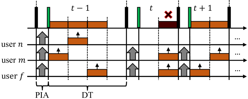
Figure 1: Example of PIMA protocol operations and its frame structure. The RB and the SB are represented by black and green rectangles, respectively; grey arrows represent the uplink signals for the user enumeration at the BS and data packets are represented by orange rectangles.

II-B Partial-Information Multiple Access Protocol

As shown in Fig. 1, each frame is divided into two sub-frames, namely the PIA sub-frame and the DT sub-frame. The PIA sub-frame is used to estimate (at the BS) the number of currently active users. Based on this information and the past statistics of successful transmissions and collisions the BS sets the duration (in slots) of the DT sub-frame and assigns each user to one slot, for possible uplink data transmission. Such scheduling information is transmitted in broadcast at the end of the PIA sub-frame. We now briefly detail the PIMA protocol, while in Section III we analyze its performance to derive policies for the slot assignment in the DT sub-frame.

Partial Information Acquisition Sub-Frame. At $\tau_{0}(t)$, the BS transmits in broadcast the RB, triggering the beginning of the PIA sub-frame and carrying the acknowledgments of correctly received packets in the previous frame. Moreover, RBs provide each user an estimate of its channel to the BS, which is subsequently used for the user enumeration. Two approaches for the PIA sub-frame are described in [16] and [14], based on a different knowledge of the channel state information at the user, and readers are referred to these papers for more details on the PIA sub-frame. Here we only recall that at the end of this phase, the BS knows (possibly with errors) the number of active users, but not their identity. Then, the BS schedules users’ transmissions for the next DT sub-frame. Let $\bm{q}(t)=[q_{1}(t),\ldots,q_{N}(t)]$ be the slot selection vector, collecting the slot indices assigned to each user. The slot selection vector is transmitted by the BS in the SB, which triggers the beginning of the following DT sub-frame. Note that the length $L_{2}(t)$ of the DT sub-frame can be derived from $\bm{q}(t)$ as $L_{2}(t)=\max_{\begin{subarray}{c}n\end{subarray}}q_{n}(t)$.

For the sake of simplicity, in the following, we assume fixed PIA sub-frame length $L_{1}$, comprehensive of both the enumeration task and the beacon transmissions, and assume an error-free user enumeration.

Data Transmission Sub-Frame. In the DT sub-frame, users transmit their buffered packets, according to the scheduling set by the BS in the SBs.

III PIMA Protocol Analysis

In this section, we describe the PIMA protocol as a PO-MDP and we introduce the latency as a penalty function to be minimized by the scheduler.

PO-MDP generalize the Markov decision processs (MDPs) by combining such models with the key features of HMMs. An HMM is defined by a Markov process, which is not directly observable (hidden process), and an observable random quantity depending only on the current state of the process (observation). PO-MDPs add the concepts of actions and penalties associated with the state transition-action couples, which are the fundamental features of MDPs. At each time period, the environment, represented here by the communication system, is in some state $i$. The agent, which is responsible to interact with the environment, takes an action, $a$, which causes the transition to state $j$ with probability $p_{i,j}(a)$. At the same time, the agent receives an observation $\bm{\beta}$ which depends on the new state of the environment $j$, and on the just taken action $a$, with emission probability $e_{\bm{\beta}}=\mathbb{P}(\bm{\beta}|a,j)$. Finally, when the system moves from state $i$ to state $j$ due to action $a$ at time $t$, the agent receives a penalty $P(t)=P(i,j,a)$, where $P(\cdot,\cdot,\cdot)$ is the penalty function. Then, the process is iterated. The goal of the agent, at each time step, aims at minimizing its expected future penalty $\mathbb{E}\left[\sum_{t=0}^{\infty}P(t)\right]$. A discount factor may be also added to balance the impact of immediate and future penalties.

Note that, differently from conventional MDP, wherein the process state is known to the agent, in PO-MDP the agent does not directly observe it, thus its actions are taken under uncertainty of the hidden state. However, by interacting with the environment and receiving observations, the agent may update its belief in the hidden state, i.e., the state probability distribution based on the observations. Therefore, as the system evolves and the environment is observed, actions are taken with a more accurate estimation of the current state.

III-A PO-MDP Model for The PIMA Protocol

In the following, we map the PIMA protocol features to each of the discussed components of a PO-MDP. For the following analysis, we assume negligible error probability in the PIA sub-frame, i.e., perfect knowledge of the number of active users, thus $\hat{\nu}(t)=\nu(t),\forall t$.

Hidden States. The hidden system state is the set of the arrival time of the packets in the buffers of all users. At time $\tau$, the state is $\bm{\mathcal{X}}(\tau)=\{x_{n,h},\forall n,h\}$, where $x_{n,h}$ is the instant of the generation of the $h$-th packet, for all packets currently in its buffer. The state space of the PO-MDP $\mathcal{Y}=\{\bm{\mathcal{X}}(\tau),\;\forall\tau\}$ has infinite cardinality, due to the infinite buffer length assumption. The buffer state evolves at each transmission attempt or packet generation, however, only the state probability at the beginning of the DT sub-frame is relevant for scheduling.

Actions. The scheduling vector $\bm{q}(t)$ is the action performed by the agent BS at frame $t$ based on its belief on the current system state. For simplicity, in the following, we denote the state at the end of the PIA sub-frame as $\bm{\mathcal{X}}(t)$.

Observations. Observations are acquired at the end of the PIA sub-frame of frame $t$ as

$$\bm{\bm{\beta}}(t)=\{\nu(t),\bm{z}(t-1),\mathcal{C}(t-1)\}\in\mathcal{O},$$ (2)

where set $\mathcal{C}(t)$ collects all slots wherein a collision is detected in frame $t$, and $\mathcal{O}$ is the set of possible observations. Note that acknowledgment and collision vectors are referred to the previous frame, as we are at the beginning of the DT sub-frame of frame $t$. The cardinality of $\mathcal{O}$ is finite, as only a limited number of combinations of successes, collisions, and number of active users may occur.

Conditional Transition Probabilities. The underlying Markov process evolves from state $\bm{\mathcal{I}}\in\mathcal{Y}$ at frame $t-1$ to state $\bm{\mathcal{J}}\in\mathcal{Y}$ with posterior conditional transition probability

$$p_{\bm{\mathcal{I}}\bm{\mathcal{J}}}(\bm{a})=\mathbb{P}\left[\bm{\mathcal{X}}(t)=\bm{\mathcal{J}}|\bm{\mathcal{X}}(t-1)=\bm{\mathcal{I}},\bm{q}(t-1)=\bm{a}\right].$$ (3)

We observe that, by imposing the condition on the observations and the previous action, transitions occur only according to the packet generation and transmission processes.

Emission Probabilities. For each state, different observations may be acquired in general. The emission probability of observing $\bm{\beta}^{\prime}$ by visiting state $\bm{\mathcal{J}}$ is defined as

$$e_{\bm{\beta}^{\prime}}(\bm{\mathcal{J}},\bm{a})=\mathbb{P}[\bm{\beta}(t)=\bm{\beta}^{\prime}|\bm{\mathcal{X}}(t)=\bm{\mathcal{J}},\bm{q}(t)=\bm{a}].$$ (4)

Beliefs. We first observe that the information at the end of the PIA sub-frame of frame $t$ is both the observations and the actions up to that frame, i.e.,

$$\mathcal{E}(t)=\{\bm{\beta}(t),\bm{\beta}(t-1),\ldots,\bm{\beta}(0),\bm{q}(t-1),\ldots,\bm{q}(0)\}.$$ (5)

Now, the belief of state $\bm{\mathcal{X}}$ is the conditional probability of being in state $\bm{\mathcal{X}}(t)$ at frame $t$, given the information available at the BS

$$\rho(\bm{\mathcal{J}},t)={\mathbb{P}}[\bm{\mathcal{X}}(t)=\bm{\mathcal{J}}|\mathcal{E}(t)].$$ (6)

The belief is recursively computed by exploiting the conditional independence of the hidden Markov chain, observing that $\mathcal{E}(t)=\{\bm{\beta}(t),\mathcal{E}(t-1)\}$ and setting the initial system conditions as

$$\rho(\bm{\mathcal{I}},0)=\begin{cases}1\quad\bm{\mathcal{I}}=\bm{0},\\ 0\quad\text{otherwise}.\end{cases}$$ (7)

The belief at the end of the PIA sub-frame of frame $t$ is computed as

$$\rho(\bm{\mathcal{J}},t)=e_{\bm{\beta}}(\bm{\mathcal{J}},\bm{a})\sum_{\bm{\mathcal{I}}:\bm{\beta}(t)=\bm{\beta}}p_{\bm{\mathcal{I}}\bm{\mathcal{J}}}(\bm{q}(t-1))\rho(\bm{\mathcal{I}},t-1).$$ (8)

Let also $\bm{\rho}(t)$ be the vector collecting $\rho(\bm{\mathcal{J}},t)$ for all $\bm{\mathcal{J}}$.

Penalty. When moving from state $\bm{\mathcal{I}}$ to state $\bm{\mathcal{J}}$ with action $\bm{a}$, the penalty is $P(\bm{\mathcal{I}},\bm{\mathcal{J}},\bm{a})$, where the penalty function depends only on the states and action.

III-B Latency As Penalty Function

As a performance metric, we consider the packet latency, which measures the time a packet spends in the buffer before successful transmission. Such time includes the delay introduced by collisions and retransmissions.

In formulas, the latency of packet $h$ in user $n$ buffer is defined as

$$D_{n,h}=\tau_{n,h}-x_{n,h},$$ (9)

where $\tau_{n,h}$ is the instant of the successful delivery of the packet to the BS. Note that all packets in user $n$ buffer at time $\tau_{0}(t)$ increase their latency by $L(t)=L_{1}+L_{2}(t)$ if they are not successfully transmitted at frame $t$. Instead, a successful transmission provides an increment of $L_{1}+q_{n}(t)$.

We consider the latency increment penalty associated with action $\bm{a}$ when in state $\bm{\mathcal{I}}$ at frame $t$, defined as

$$P(\bm{\mathcal{I}},\bm{\mathcal{J}},\bm{q}(t))=\sum_{n=1}^{N}\sum_{h=1}^{K_{n}(\tau_{0}(t))}d_{n,h}(t),$$ (10)

where the incremental latency of packet $h$ in user $n$ buffer is

$$d_{n,h}(t)=\begin{cases}L_{1}+q_{n}(t-1),&h=1,\;z_{n}(t-1)=1,\\ L(t-1),&z_{n}(t-1)=0,\\ \tau_{0}(t)-x_{n,h}&\text{otherwise},\end{cases}$$ (11)

and we note that from the couple of subsequent states $\bm{\mathcal{I}},\bm{\mathcal{J}}$ at frames $t$ and $t+1$ we can compute $\bm{z}(t)$. Since we consider FIFO buffers, $h=1$ refers to the oldest packet in the buffer, which is also the first scheduled for transmission in the buffer.

III-C PO-MDP Solution

As for conventional MDPs, the solution of the PO-MDP minimizes the expected future penalty $\mathbb{E}\left[\sum_{t=0}^{\infty}P(t)\right]$. Note that, since the agent does not directly observe the environment’s state, it must make decisions based on its belief of the current state. For this reason, the PO-MDP is typically formulated as a conventional infinite-states MDP by moving from space $\mathcal{Y}$ to the continuous space of all distributions of the beliefs, thus all possible values of $\rho(\bm{\mathcal{J}})$, for all $\bm{\mathcal{J}}\in\mathcal{Y}$. Both the observations and actions are the same of the original PO-MDP, and the policy function maps each belief state to an action,

$$\pi:\bm{\rho}(t)\rightarrow\bm{q}(t).$$ (12)

The optimal policy, i.e, the one minimizing the long-term penalty, is the solution of the Bellman equation applied to the belief MDP, as detailed in [17].

IV Frame-Efficiency Optimization

The direct PO-MDP solution is, in general, very challenging, due to the infinite number of hidden states of the PO-MDP model. Therefore, we consider a sub-optimal solution that determines the frame length $L_{2}(t)$ iteratively, while performing the user assignments. To this end, we first resort to the frame efficiency metric [14], which can be extended to the correlated activation case exploiting the PO-MDP formulation.

Let $l\in\{1,\ldots,L_{2}(t)\}$ be the slot index within frame $t$ (in the DT sub-frame), and let $c_{l}=1$ if a successful transmission occurs at slot $l$ and $c_{l}=0$ otherwise. The conditional frame efficiency is defined as

$$\eta(t)=\frac{1}{L_{2}(t)}\sum_{l=1}^{L_{2}(t)}\mathbb{E}[c_{l}|\mathcal{E}(t)],$$ (13)

where, with respect to the definition in [14], the condition on $\mathcal{E}(t)$ accounts for the transmission outcomes history.

At frame $t$, immediately after the end of the PIA sub-frame, the BS solves the following optimization problem:

$$\max_{\begin{subarray}{c}\bm{q}(t)\end{subarray}}\eta(t),$$ (14a)

$${\rm s.t.\;}\;\;q_{n}(t)\in\{1,\ldots,L_{2}(t)\}.$$ (14b)

Still, problem (14) is one of mixed integer non-linear programming (MINLP), and its solution quickly becomes for large numbers of users. Therefore, to simplify the analysis, we resort to a greedy scheduling solution.

IV-A Greedy Frame Efficiency Optimizer Algorithm

The proposed algorithm is denoted as greedy frame efficiency optimizer (GFEO) algorithm, and it iteratively adjusts the frame length $L_{2}(t)$, while performing the user assignments $\bm{q}(t)$. First, note that, due to the assumption of buffering packets generated during frame $t$ and single slot assignment to each user, each hidden state/action couple leads to a single possible observation $\bm{\beta}^{*}$. Thus, the emission probability is $e_{\bm{\beta}}(\bm{\mathcal{J}},\bm{a})=1$, for $\bm{\beta}=\bm{\beta}^{*}$, and $e_{\bm{\beta}}(\bm{\mathcal{J}},\bm{a})=0$ otherwise. Hence, (8) can be rewritten and recursively computed as

$$\rho(\bm{\mathcal{J}},t)=\sum_{\bm{\mathcal{I}}:\bm{\beta}(t)=\bm{\beta}^{*}}p_{\bm{\mathcal{I}}\bm{\mathcal{J}}}(\bm{q}(t-1))\rho(\bm{\mathcal{I}},t-1).$$ (15)

Now, let $\eta(L_{2}(t),\bm{q}(t))=\eta(t)$ be the expected conditional frame efficiency, where we now highlight its dependence on the DT sub-frame length and the user assignment. Let us also introduce the activation probability of user $n$ conditioned to the current belief states, i.e., from (15),

$$\phi_{n}(t)=\sum_{\bm{\mathcal{I}}:K_{n}(\tau_{0}(t))>0}\rho(\bm{\mathcal{I}},t).$$ (16)

Finally suppose, without loss of generality, that users’ indices are ordered with decreasing activation probability, i.e.,

$$\phi_{1}(t)\geq\phi_{2}(t)\geq\ldots\geq\phi_{N}(t).$$ (17)

The GFEO algorithm includes $N$ iterations (one per user), assigning user $n$ to a specific time slot at iteration $n$. At the first iteration ($n=1$), user 1 is assigned to the first DT slot of the frame, i.e., $q_{1}(t)=1$.

The algorithm compares the frame efficiency obtained by assigning the current user to each of the already allocated slots, or to a new slot, thus increasing $L_{2}(t)$. Then, the best solution among those explored is chosen, and the algorithm moves to the scheduling of the next user. Specifically, at iteration $n\geq 2$, the algorithm computes the conditional frame efficiency obtained by assigning user $n$ to each slot $l\in\{1,\ldots,L_{2}(t)\}$. Letting $q_{m}(t)$, $m=1,\ldots,n-1$, be the indices of the slots assigned to the previous $n-1$ users, the GFEO assigns user $n$ to the slot with index

$$\begin{split}q_{n}(t)=\operatorname*{\arg\!\max}_{\ell}\left\{\max\left[\eta(L_{2}(t),\tilde{\bm{q}}_{n}(l,t)),\right.\right.\\ \left.\left.\eta(L_{2}(t)+1,\tilde{\bm{q}}_{n}(l,t))\right]\right\},\end{split}$$ (18)

where $\tilde{\bm{q}}_{n}(l,t)=[q_{1}(t),\ldots,q_{n-1}(t),l,0,\ldots,0]$. The frame length $L_{2}(t)$ is updated at each iteration, depending on the frame efficiency provided by each assignment. Note that the BS exploits only the partial information acquired through the observation history, while the instantaneous state of the hidden Markov process is never exploited, as the BS has no knowledge of the buffers conditions. Thus, in general, this algorithm provides a sub-optimal policy.

Practical MDP Considerations. Due to the potentially infinite state space provided by the arrival instants of the packets in the users’ buffers, it is impossible to compute (16) in practice. As a first approximation, instead of considering the state of the arrival instants, we consider the state of the buffers load, i.e., the state is described by the number of packets in each user’s buffer. Still, under the assumption of infinite buffer capacities, the state space remains infinite. Nevertheless, we can assume finite buffers of length $C$ and analyze the system in stability conditions, wherein the number of packets in each user is always less than $C$ in practice. Under this further assumption, the total number of PO-MDP states is $|\mathcal{Y}|=(C+1)^{N}$.

IV-B Simplified GFEO

Although being extremely accurate in the estimation of the users’ buffer states and their correlation, due to the memory of the previous observations, the PO-MDP model quickly becomes unfeasible with the increasing number of users in the system. In particular, as the number of states increases exponentially with $N$, the complexity of the computation of the posterior probabilities (15) drastically increases.

To overcome this limitation, we further simplify the state space and consider a low-complexity variant of the proposed greedy scheduler, named simplified GFEO (S-GFEO). With S-GFEO, at frame $t$ the recursion in (15) is removed by considering $\mathcal{E}(t)=\{\bm{\beta}(t),\nu(t-1)\}$, i.e., only the observation of frame $t-1$ and not the entire history of actions and observations. Under this assumption, the memory of the state transitions is not kept, and the computation of $\rho(\bm{\mathcal{I}},t-1)$ is avoided by setting a uniform distribution of the states compatible with the current observation $\mathcal{E}(t)$. Let $\mathcal{Z}(t)=\{\bm{\mathcal{I}}:\mathcal{E}(t)=\bm{\beta}^{*}\}$ be the set of state compatible with observation $\bm{\beta}^{*}$, the posterior probabilities at frame $t$ are computed from (8) and (15) as

$$\rho(\bm{\mathcal{J}},t)=\sum_{\bm{\mathcal{I}}\in\mathcal{Z}}p_{\bm{\mathcal{I}}\bm{\mathcal{J}}}(\bm{q}(t-1))\frac{1}{|\mathcal{Z}(t)|}.$$ (19)

Then, S-GFEO proceeds with the users’ scheduling as GFEO.

V Numerical Results

In this section, we present the numerical results, comparing the GFEO and S-GFEO schedulers with a) the time-division multiple-access (TDMA), providing fixed-duration frames of $N$ slots with one user assigned per slot deterministically, b) the Rivest’s stabilized SALOHA [7], wherein users generating packets are backlogged with the same probability, and c) the PIMA protocol of [14]. For all schemes, we adopt the third numerology of the new radio (NR) specification, which provides DT time slots of $T_{\rm s}=0.125$ ms [18]. Moreover, for PIMA, GFEO, and S-GFEO, we assume an error-free user enumeration with a fixed $L_{1}$.

The performance is assessed in terms of average frame efficiency $\bar{\eta}$ (conditioned on $\nu(t)>0$), and average latency $\bar{D}=\mathbb{E}[D_{n,h}]$, computed from all successfully delivered packets.

Figure 2: Average frame efficiency versus the total arrival rate for $N=5$. The zoom plot inside the figure highlights the performance gap between the PIMA-based schedulers.

Figure 3: Average packet latency versus the packet arrival rate for $N=5$.

Firstly, we consider a scenario with $N=5$ users with traffic intensity $0.01\leq\Lambda\leq 0.5$, which corresponds to the queues’ stability regime of the GFEO algorithm, which has been derived empirically from the simulations. The length of the PIA sub-frame is set to $L_{1}=T_{\rm s}/10$, which is sufficient to guarantee negligible enumeration error probability [14]. Fig. 2 shows the average frame efficiency $\bar{\eta}$ as a function of the total packet generation rate. Note that the performance of SALOHA is not reported, as the frame efficiency cannot be defined for frame-less protocols SALOHA. TDMA, adopting the constant maximum frame length, provides a very low frame efficiency, while the PIMA-based schedulers attain close-to-optimal performance in the whole considered range of traffic intensity. Among these schedulers, GFEO, which exploit the correlation knowledge at best, achieve the highest frame efficiency providing approximately up to 5% gain with respect PIMA. However, the results also show that the gap between GFEO and S-GFEO is almost negligible, therefore the approximations introduced with S-GFEO have a very limited negative impact on the system performance. Finally, while the frame efficiency is increasing with the traffic intensity for TDMA due to the reduced unused time slots, it is slightly decreasing for the PIMA-based schemes due to the increasing chances of collisions.

The comparison of the average packet latency is shown in Fig. 3. At low traffic, TDMA provides the larger latency due to the frame length fixed to $N$, while SALOHA achieves extremely low latency due to the absence of collisions. Instead, at high traffic intensity, the SALOHA backlogging mechanism prevents the users to transmit their buffered packets immediately, therefore increasing the average latency. The PIMA-based schemes, due to their better capability of adapting to traffic conditions, outperform both schemes when the traffic intensity is moderately large. In particular, both GFEO and S-GFEO achieve the lowest latency, still with an almost negligible gap between these greedy solutions.

Figure 4: Average packet latency versus the packet arrival rate for $N=30$.

Finally, we consider a scenario with $N=30$ users and a fixed PIA sub-frame length $L_{1}=T_{\rm s}/4$. Here, the performance of GFEO is not reported due to its extremely high complexity for a large number of users. However, we have observed that its low-complexity variant S-GFEO scales better at the cost of a negligible loss in performance. Fig. 4 depicts the average packet latency achieved by the compared schemes. First, note that similarly to Fig. 3, the results show a huge latency reduction of the PIMA-based solutions with respect to the other considered schenes. We stress that the average latency counts only for the successfully delivered packets and that we are considering values of $\Lambda$ such that the queues’ stability is verified for PIMA and GFEO. Therefore, while TDMA seems to outperform PIMA at high traffic, this is only due to the instability conditions of TDMA, which drops the oldest packets in the users’ queues when the maximum capacity is reached. Still, we observe that S-GFEO achieves the lowest latency among all the compared schemes.

VI Conclusions

To minimize the latency of our recently proposed PIMA scheme, we proposed to model the protocol with a PO-MDP. The scheduling is optimized based on the knowledge of both the number of active users and past transmission outcomes, which are mapped to the observation of a hidden Markov process. To overcome the huge complexity of the scheduling problem, we proposed two sub-optimal greedy schedulers namely GFEO and S-GFEO, both aiming at dynamically maximizing the frame efficiency. Numerical results show the effectiveness of both GFEO and S-GFEO in attaining extremely low latency over a wide range of traffic intensity.

References

- [1] Y. Saito, Y. Kishiyama, A. Benjebbour, T. Nakamura, A. Li, and K. Higuchi, “Non-orthogonal multiple access (NOMA) for cellular future radio access,” in Proc. VTC Spring, 2013, pp. 1–5.
- [2] L. Dai, B. Wang, Z. Ding, Z. Wang, S. Chen, and L. Hanzo, “A survey of non-orthogonal multiple access for 5G,” IEEE Commun. Surveys Tuts., vol. 20, no. 3, pp. 2294–2323, 2018.
- [3] Y. Chen et al., “Toward the standardization of non-orthogonal multiple access for next generation wireless networks,” IEEE Commun. Mag., vol. 56, no. 3, pp. 19–27, Mar. 2018.
- [4] Y. Polyanskiy, “A perspective on massive random-access,” in Proc. IEEE ISIT, 2017, pp. 2523–2527.
- [5] A. Decurninge, I. Land, and M. Guillaud, “Tensor-based modulation for unsourced massive random access,” IEEE Wireless Commun. Lett., vol. 10, no. 3, pp. 552–556, Oct. 2020.
- [6] A. Rech, A. Decurninge, and L. G. Ordóñez, “Unsourced random access with tensor-based and coherent modulations,” arXiv preprint arXiv:2304.12058, 2023.
- [7] R. Rivest, “Network control by bayesian broadcast,” IEEE Trans. Inf. Theory, vol. 33, no. 3, pp. 323–328, May 1987.
- [8] A. E. Kalør, O. A. Hanna, and P. Popovski, “Random access schemes in wireless systems with correlated user activity,” in Proc. IEEE SPAWC, 2018, pp. 1–5.
- [9] F. Moretto, A. Brighente, and S. Tomasin, “Greedy maximum- throughput grant-free random access for correlated IoT traffic,” in Proc. VTC Fall, 2021, pp. 1–5.
- [10] A. Rech and S. Tomasin, “Coordinated random access for industrial IoT with correlated traffic by reinforcement-learning,” in Proc. IEEE GLOBECOM WKSHPS, 2021, pp. 1–6.
- [11] A. Destounis, D. Tsilimantos, M. Debbah, and G. S. Paschos, “Learn2MAC: Online learning multiple access for URLLC applications,” in Proc. IEEE INFOCOM WKSHPS, vol. Apr., 2019, pp. 1–6.
- [12] G. Wunder, P. Jung, and C. Wang, “Compressive random access for post-LTE systems,” in Proc. IEEE ICC WKSHPS, 2014, pp. 539–544.
- [13] J. Choi, “On throughput of compressive random access for one short message delivery in IoT,” IEEE Internet Things J., vol. 7, no. 4, pp. 3499–3508, Jul. 2020.
- [14] A. Rech, S. Tomasin, L. Vangelista, and C. Costa, “Partial-information multiple access protocol for orthogonal transmissions,” Proc. International Conference on Ubiquitous and Future Networks (ICUFN), 2023. [Online]. Available: arXiv preprint arXiv:2304.12057
- [15] M. Goldenbaum and S. Stanczak, “Robust analog function computation via wireless multiple-access channels,” IEEE Trans. Commun., vol. 61, no. 9, pp. 3863–3877, Sep. 2013.
- [16] A. Rech, S. Tomasin, L. Vangelista, and C. Costa, “Semi-grant-free orthogonal multiple access with partial-information for short packet transmissions,” arXiv preprint arXiv:2307.14846, 2023.
- [17] L. P. Kaelbling, M. L. Littman, and A. R. Cassandra, “Planning and acting in partially observable stochastic domains,” Artificial Intelligence, vol. 101, no. 1, pp. 99–134, Jan. 1998.
- [18] 3GPP, “5G-NR; physical channels and modulation,” 3rd Generation Partnership Project (3GPP), Technical Report (TR) 38.211, 7 2020, version v.16.2.0.