Thermodynamics of interacting systems: the role of the topology and collective effects

Abstract

We will study a class of system composed of interacting unicyclic machines placed in contact with a hot and cold thermal baths subjected to a non-conservative driving worksource. Despite their simplicity, these models showcase an intricate array of phenomena, including pump and heat engine regimes as well as a discontinuous phase transition. We will look at three distinctive topologies: a minimal and beyond minimal (homogeneous and heterogeneous interaction structures). The former case is represented by stark different networks (“all-to-all” interactions and only a central interacting to its neighbors) and present exact solutions, whereas homogeneous and heterogeneous structures have been analyzed by numerical simulations. We find that the topology plays a major role on the thermodynamic performance for smaller values of individual energies, in part due to the presence of first-order phase-transitions. Contrariwise, the topology becomes less important as individual energies increases and results are well-described by a system with all-to-all interactions.

I Introduction

The study of thermal engines has always been a central part of thermodynamics Carnot (1978); Curzon and Ahlborn (1975). In particular, the last couple of decades have seen a surge of interest in the thermodynamics of thermal engines due to the emergence of stochastic thermodynamics Seifert (2012); Van den Broeck and Esposito (2015). One can for example think about the maximization of power and efficiency Verley et al. (2014); Schmiedl and Seifert (2007); Cleuren et al. (2015); Van den Broeck (2005); Esposito et al. (2010); Seifert (2011); Izumida and Okuda (2012); Golubeva and Imparato (2012); Holubec (2014); Bauer et al. (2016); Proesmans et al. (2016a); Tu (2008); Ciliberto (2017); Bonança (2019); Mamede et al. (2022); Proesmans et al. (2016b); and the influence of studies of system-bath coupling Noa et al. (2021); Harunari et al. and the level of control Guéry-Odelin et al. (2019); Deffner and Bonança (2020); Pancotti et al. (2020); Zhao et al. (2022).

One particularly interesting idea is that systems performance might be enhanced by collective effects such as phase-transitions Hooyberghs et al. (2013); Campisi and Fazio (2016). These types of collective behavior, e.g., order-disorder phase transitions Yeomans (1992) and synchronization Torres et al. (2005); Tönjes et al. (2021), have been observed in a broad range of systems such as complex networks Bonifazi et al. (2009); Schneidman et al. (2006); Buzsáki and Mizuseki (2014); Gal et al. (2017), biological systems Rapoport (1970); Gnesotto et al. (2018); Lynn et al. (2021); Smith and Schuster (2019) and quantum systems Mukherjee and Divakaran (2021); Niedenzu and Kurizki (2018); Kurizki et al. (2015); Lee et al. (2022); Campisi and Fazio (2016); Mukherjee et al. (2020); Halpern et al. (2019); Kim et al. (2022); Kolisnyk and Schaller (2023); Latune et al. (2019); Chen et al. (2019).This has inspired the development of theoretical models of thermodynamic engines, in which the performance can be boosted via collective effects. Most of these models, however, focus on either one-dimensional systemsMamede et al. (2022); Fogedby and Imparato (2017); Imparato (2021); Suñé and Imparato (2019) or mean-field like models Vroylandt et al. (2017, 2020); Herpich et al. (2018); Herpich and Esposito (2019); Filho et al. (2023). Little is known about the influence that network topology might have on system performance.

This paper aims to partially fill this gap, by studying the influence of topology of a simple class of system, composed of interacting units, referred to here as a collection of nanomachines, placed in contact with a hot and cold ther- mal baths subjected to a non-conservative driving worksource. The approach to be considered here is akin to the commonly referred to as ”lattice-gas” models in the realm of equilibrium statistical mechanics. They have a longstanding importance in the context of collective effects and serving as the corner- stone for numerous theoretical, experimental, and technological breakthroughs, encompassing the ferromagnetism, liquid phases, the topology effect, the fluctuation-driven generation of new phases and others, highlighting that distinct systems have been described/characterized via Hamiltonian of the fundamental models (e.g., the Ising, Potts, XY and Heisenberg models). The all-to-all version for our model has been investigated previously Cleuren and Van den Broeck (2001); Vroylandt et al. (2017, 2020) for finite and infinite number of interacting units, in which the cooperative effect gives rise to a rich behavior, including the enhancement of the power and efficiency at optimal interactions, the existence of distinct operation models and a discontinuous phase transition. Furthermore, systems with all-to-all interaction can be solved analytically, which makes them easier to analyze. There are, however, also many systems where systems only interact locally (nearest-neighbor like).

In this paper, we present a detailed study on the influence of the topology in aforementioned class of interacting units. We will focus on two distinctive approaches: minimal models, which can be treated analytically, and more complicated systems, where we will focus on numerical analysis. In the former class, we will focus on systems with all-to-all interaction and a one-to-all interaction (also known as stargraph), in which a single central spin is interacting with all other units. After that, we go beyond the minimal models by considering the influence of homogeneous and heterogeneous interaction topologies. We will show that, for small values of individual energies $\beta_{\nu}\epsilon$ of each occupied unit, the lattice topology can have a significant influence on the system performance, in which the increase of interaction $V$ among units can give rise to a discontinuous phase transition. Conversely, as $\beta_{\nu}\epsilon$ increases, the phase transition is absent and the topology plays no crucial role and the models seem mutually similar. In this case one can get approximate expressions for thermodynamic quantities through a phenomenological two-state model.

The paper is structured as follows: in Section II, we introduce the model and its thermodynamics. Section III describes the lattice topologies which will be analysed. In Section IV, the aforementioned minimal models are studied. In Section V, the more complicated topologies are studied. Conclusions are drawn in Section VI.

II Model and Thermodynamics

We are assuming a system composed of $N$ interacting two-state nanomachines. The two states of each individual machine are denoted as $\sigma_{i}=0(1)$ according to whether it occupies the lower(upper) state with energy $0(\epsilon)$. We will consider that the system is in contact with two thermal baths at different temperatures. Furthermore, there will be a non-conservative force (described below) that extracts work from the system, in this way creating a thermal engine. The state of the full system is then described by $\sigma\equiv(\sigma_{1},\sigma_{2},...,\sigma_{i},...,\sigma_{N})$, where $\sigma_{i}$ describes the state of the $i$’th machine. Throughout this paper, we shall restrict our analysis on transitions between configurations $\sigma$ and $\sigma^{i}$ differ by the state of one machine, namely that of unit $i$. In this case, the time evolution of probability $p(\sigma,t)$ satisfies a master equation,

$${\dot{p}}(\sigma,t)=\sum_{\nu=1}^{2}\sum_{i=1}^{N}\{\omega_{i}^{(\nu)}(\sigma^{i})p(\sigma^{i},t)-\omega_{i}^{(\nu)}(\sigma)p(\sigma,t)\},$$ (1)

where $\sigma^{i}\equiv(\sigma_{1},...,1-\sigma_{i},...,\sigma_{N})$ and index $\nu=1(2)$ accounts for transitions induced by the cold (hot) thermal bath. The transition rate due to the contact with the $\nu$-th thermal bath are assumed to be of Arrhenius form

$$\omega_{i}^{(\nu)}(\sigma)=\Gamma e^{-\frac{\beta_{\nu}}{2}\{E_{a}+{\Delta E}_{i}(\sigma)+F_{\nu}\}},$$ (2)

where ${\Delta E}_{i}(\sigma)$ is the difference of energy between states $\sigma^{i}$ and $\sigma$ and $\Gamma e^{-\beta_{\nu}E_{a}/2}$ accounts to the coupling between the QD and thermal bath, expressed in terms of the activation energy $E_{a}$ and $\beta_{\nu}=1/T_{\nu}$, [hereafter we shall adopt $k_{B}=1$]. As stated previously, the interaction among units will depend on the lattice topology, whose energy of system is given by the generic expression:

$$E(\sigma)=\epsilon n+\sum_{i=1}^{N}\frac{V}{\langle k\rangle}\sum_{j=1}^{k_{i}}(\delta_{\sigma_{i},1-\sigma_{i+j}}+\delta_{1-\sigma_{i},\sigma_{i+j}}),$$ (3)

where $n=\sum_{i=1}^{N}\sigma_{i}$ denotes the total number of units in the state of energy $\epsilon$, $V$ is the interaction strength ($\delta$ being the Kronecker delta) and $\langle k\rangle$ is the average number of neighbours to which each unit is connected. Eq. (3) has been inspired by earlier studies about interacting system, in which a similar type of interaction is consider to describe the interaction between nanomachines in distinct states Vroylandt et al. (2017, 2020). Also, this interaction shares some similarities with recent papers Prech et al. (2023); Cuetara and Esposito (2015) in which the tunneling between two quantum-dots is investigated via the inclusion of a similar term. We will both look at topologies where $k_{i}$, the number of nearest neighbors of the unit $i$ is independent of $i$, $\langle k\rangle=k_{i}$ (all-to-all interactions and homogeneous systems) and cases where $k_{i}$ depends on $i$ (stargraph and heterogeneous systems). One of these earlier studies also used similar types of work sources: we consider the worksource given by $F_{\nu}$ with $F_{\nu}=(-1)^{\nu}(1-2\sigma_{i})F$, in such a way that transitions $0\rightarrow 1$ ($1\rightarrow 0$) are favored according to whether the system is placed in contact with the cold (hot) thermal baths. This type of interaction can also be mapped on other types of systems such as kinesin Liepelt and Lipowsky (2007, 2009), photo-acids Berton et al. (2020) and ATP-driven chaperones De Los Rios and Barducci (2014).

From Eq. (1) together transition rates given by Eq. (2), the time evolution of mean density $\rho=\langle\sigma_{i}\rangle$ and mean energy $\langle E(\sigma)\rangle=\sum_{\sigma}E(\sigma)p(\sigma,t)$ obey the following expressions:

$${\dot{\rho}}=\langle(1-2\sigma_{i})(\omega^{(1)}_{i}(\sigma)+\omega^{(2)}_{i}(\sigma))\rangle,$$ (4)

and

$$\frac{d}{dt}\langle E(\sigma)\rangle={\cal P}+\langle\dot{Q}_{1}\rangle+\langle\dot{Q}_{2}\rangle,$$ (5)

respectively, where ${\cal P}$ and $\langle\dot{Q}_{\nu}\rangle$ denote the mean power and the heat exchanged with the $\nu$-th thermal bath and are given by Vroylandt et al. (2017); Filho et al. (2023):

$${\cal P}=F\sum_{i=1}^{N}\left\langle\omega^{(1)}_{i}(\sigma)-\omega^{(2)}_{i}(\sigma)\right\rangle,\\$$ (6)

and

$$\langle\dot{Q}_{\nu}\rangle=\langle(\Delta E_{i}(\sigma)+F(-1)^{(\nu)})\omega_{i}^{(\nu)}(\sigma)\rangle,$$ (7)

the standard stochastic thermodynamics expressions for power and heat respectively Seifert (2012).

Throughout this paper, we will assume that the system has relaxed to a steady state, $p(\sigma,t)\rightarrow p^{st}(\sigma)$, i.e., ${\cal P}+\langle\dot{Q}_{1}\rangle+\langle\dot{Q}_{2}\rangle=0$. In this case, one can also write the entropy production as

$$\langle{\dot{\sigma}}\rangle=\sum_{\nu=1}^{2}\sum_{\sigma}\sum_{i=1}^{N}\,{J}^{(\nu)}(\sigma^{i})\log\frac{\omega^{(\nu)}_{i}(\sigma^{i})}{\omega^{(\nu)}_{i}(\sigma)},$$ (8)

with ${J}^{(\nu)}(\sigma^{i})=\omega^{(\nu)}_{i}(\sigma^{i})p^{\rm st}(\sigma^{i})-\omega^{(\nu)}_{i}(\sigma)p^{\rm st}(\sigma)$. One can verify from Eq. (2) that the entropy production, Eq. (8) assumes the classical form $\langle{\dot{\sigma}}\rangle=-\beta_{1}\langle\dot{Q}_{1}\rangle-\beta_{2}\langle\dot{Q}_{2}\rangle$, in similarity with equilibrium thermodynamics.

Under the correct choice of parameters, an amount of heat extracted from the hot bath $\langle\dot{Q}_{2}\rangle>0$ can be partially converted into power output ${\cal P}<0$ and the system can be used as a heat engine. The efficiency is then defined as $\eta=-{\cal P}/\langle\dot{Q}_{2}\rangle$, which satisfy the classical relation $\eta\leq\eta_{c}=1-\beta_{2}/\beta_{1}$.

III Lattice Topologies

As stated in the previous section, we intend to study the differences in thermodynamic quantities between topologies. We will focus on two classes of systems: Minimal structures, namely stargraph and all-to-all interacting systems, and beyond minimal structures, comprising homogeneous and heterogeneous systems. In stargraph systems the interactions are restricted to a central unit(hub) which interacts with its all nearest neighbor sites (leaves).

Homogeneous and heterogeneous structures present remarkably different properties and has been subject of extensive investigation. While the former case have been largely studied for addressing the main properties of graphs, the latter describes a broad class of systems, such as ecosystems, the Internet, the spreading of rumors and news, citations and others, in which the agents form heterogeneous networks and are approximately scale-free, containing few nodes (called hubs) with unusually high degree as compared to the other nodes of the network. For the homogeneous case, we shall consider those characterized by a fixed neighborhood per unit, being grouped out in two categories, including a regular arrangement (interaction between nearest neighbors) or a random-regular structure, in which all units have the same number of nearest neighbors, but they are randomly distributed. Such latter case is commonly generated through a configurational by Bollobás Bollobás (1980). Finally, among the distinct heterogeneous structures, we will consider the Barabasi–Albert scale-free network, being probably the most well-known example of heterogeneous networks Barabási and Albert (1999). The Barabási–Albert (BA) model is based on a preferential attachment mechanism, in which the degree distribution follows a power-law with scaling exponent $\gamma=3$ Barabási and Albert (1999).

IV Minimal models for collective effects: All-to-all interactions versus stargraph

We will first look at the thermodynamic properties of “all-to-all” and stargraph minimal topologies. There are several reasons for this. First, both of these models can in principle be solved exactly. Second, these structures can be seen as each others opposite. Third, the thermodynamic properties stargraph topologies can give some insights about heterogeneous networks (e.g. Barabasi-Albert), in a which some nodes are highly connected and most the remaining ones have few connections Barrat et al. (2008); Tönjes et al. (2021); Vlasov et al. (2015).

IV.1 Steady-state distribution

For an all-to-all topology, the state of the system is fully characterized by the number of units in the upper state, $n=\sum_{i=1}^{N}\sigma_{i}$. In terms of total occupation, the master equation for the all-to-all system simplifies to

$$\centering\dot{p}(n,t)=\sum_{\nu=1}^{2}\sum_{\alpha\in\{-1,1\}}[\omega^{(\nu)}_{n,n+\alpha}p(n+\alpha,t)-\omega^{(\nu)}_{n+\alpha,n}p(n,t)],\@add@centering$$ (9)

The steady-state distribution for $p^{st}(n)$ then satisfies Vroylandt et al. (2017)

$$\centering p^{st}(n)=\frac{1}{Z}\left[\prod_{m=0}^{n-1}\omega_{m+1,m}\right]\left[\prod_{m=n+1}^{N}\omega_{m-1,m}\right],\@add@centering$$ (10)

where $Z$ is the normalization factor and $\omega_{ij}=\sum_{\nu=1}^{2}\omega^{(\nu)}_{ij}$, with transition rates solely expressed in terms of $n$ by $\omega_{m+1,m}^{(\nu)}=\Gamma(N-m)e^{-\frac{\beta_{\nu}}{2}\{E_{a}+\epsilon+{\Delta E}+(-1)^{\nu}F\}}$ and $\omega_{m-1,m}^{(\nu)}=\Gamma me^{-\frac{\beta_{\nu}}{2}\{E_{a}-\epsilon-{\Delta E}-(-1)^{\nu}F\}}$ with $\Delta E=Vm(N-m)/N$. The thermodynamic quantities can be evaluated from the probability distribution such that,

$${\cal P} = F\sum_{n=0}^{N-1}(J^{(1)}_{n+1,n}-J^{(2)}_{n+1,n}),$$ (11)

$$\langle\dot{Q}_{\nu}\rangle = \sum_{n=0}^{N-1}\left[\epsilon+\Delta E+(-1)^{\nu}F\right]J^{(\nu)}_{n+1,n},$$ (12)

expressed in terms of the probability current $J^{(\nu)}_{n+1,n}=\omega_{n+1,n}^{(\nu)}p^{st}(n)-\omega_{n,n+1}^{(\nu)}p^{st}(n+1)$. An overview of the model features in all-to-all topologies will be depicted next (see e.g. Figs. 2 and Refs.Vroylandt et al. (2017, 2020)), being strongly dependent on the interplay between individual $\epsilon$ and interaction $V$ parameters. For $\beta_{\nu}\epsilon<<1$, the increase of interaction strength $V$ favors a full occupation of units in the upper state $\rho\rightarrow 1$, whereas $\rho$ exhibits a monotonous decreasing behavior upon $V$ is raised for $\beta_{\nu}\epsilon>>1$. The crossover between above regimes yields for finite $\epsilon$ and depends on $E_{a},\beta_{1}/\beta_{2}$ and $F$. Another important point to be highlighted concerns that as $E_{a}$ is increased and $\beta_{\nu}\epsilon$ is small, the interaction marks two distinct trends of the density: its decreasing behavior of prior the threshold interaction followed by sharp increase towards $\rho\rightarrow 1$ at $V=V_{0}$ [see also e.g. Fig.2$(a)$]. Such behavior corresponds to a discontinuous phase transition (see e.g. Fig. 6)$(a)$. In Sec. IV.2, we shall investigate these consequences over the system performance.

It is in principle possible to calculate the exact steady-state distribution for a finite-size star-graph by diagonalising the evolution matrix. However, some insights into the dynamics can be obtained by doing appropriate approximations, as we will show now. First, we note that the state of the system can be written in terms of $n$ and $c$, denoting the number of leaves and the hub in the upper state, respectively. The associated probability distribution, $p(n,c,t)$, satisfies

$$\centering\dot{p}(c,n,t)=\sum_{\nu=1}^{2}\sum_{\alpha\in\{-1,1\}}\left(\mathcal{J}^{(c,\nu)}_{n,\alpha}(t)+\mathcal{K}^{(n,\nu)}_{c}(t)\right),\@add@centering$$ (13)

where

$$\centering\mathcal{J}^{(c,\nu)}_{n,\alpha}(t)\equiv\omega^{(c,\nu)}_{n,n+\alpha}p(c,n+\alpha,t)-\omega^{(c,\nu)}_{n+\alpha,n}p(c,n,t),\@add@centering$$ (14)

and

$$\centering\mathcal{K}^{(n,\nu)}_{c}(t)=\kappa^{(n,\nu)}_{c,1-c}p(1-c,n,t)-\kappa^{(n,\nu)}_{1-c,c}p(c,n,t),\@add@centering$$ (15)

with $n=0,1,...,N-1$ and transition rates rewritten in the following way

$$\omega^{(c,\nu)}_{n+1,n} = \Gamma(N-1-n)e^{-\frac{\beta_{\nu}}{2}\left[E_{a}+\epsilon+V(1-2c)+F(-1)^{\nu}\right]},$$ (16)

$$\omega^{(c,\nu)}_{n-1,n} = \Gamma ne^{-\frac{\beta_{\nu}}{2}\left[E_{a}-\epsilon-V(1-2c)-F(-1)^{\nu}\right]},$$ (17)

$$\kappa^{(n,\nu)}_{1-c,c} = \Gamma e^{-\frac{\beta_{\nu}}{2}\left\{E_{a}+(1-2c)[V(N-1-2n)+\epsilon]+F(-1)^{\nu}\right\}}.$$ (18)

We assume that the hub dynamics evolves into a faster time-scales than the relaxation of the surrounding leaves, in such a way that it can be assumed/treated as thermalized at a local leaf transition $n\pm 1$. In other words transitions are such that $(\kappa^{(n,1)}_{0,1}+\kappa^{(n,2)}_{0,1})p(1|n)=(\kappa^{(n,1)}_{1,0}+\kappa^{(n,2)}_{1,0})p(0|n)$ and hence, the joint probability $p^{st}(1|n)$ is given by:

$$p^{st}(1|n)=\frac{\kappa^{(n,1)}_{1,0}+\kappa^{(n,2)}_{1,0}}{\kappa^{(n,1)}_{1,0}+\kappa^{(n,2)}_{1,0}+\kappa^{(n,1)}_{0,1}+\kappa^{(n,2)}_{0,1}},$$ (19)

where $p^{st}(0|n)=1-p^{st}(1|n)$. By summing Eq. (13) over $c$, together the property $p(n,c)=p(c|n)p(n)$, one arrives at the following equation for the time evolution of probability $p(n,t)$

$${\dot{p}}(n,t)=\sum_{\nu=1}^{2}\sum_{\alpha\in\{-1,1\}}\mathbf{\pi}^{(\nu)}_{n,n+\alpha}p(n+\alpha,t)-\mathbf{\pi}^{(\nu)}_{n+\alpha,n}p(n,t),$$ (20)

where

$$\mathbf{\pi}^{(\nu)}_{n+\alpha,n}=p^{st}(0|n)\omega^{(0,\nu)}_{n+\alpha,n}+p^{st}(1|n)\omega^{(1,\nu)}_{n+\alpha,n}.$$ (21)

Since Eq. (20) is analogous to Eq. (9) for the all-to-all case, the probability distribution of leaves $p^{st}(n)$ is given by

$$p^{st}(n)=\frac{1}{Z}\left[\prod_{m=0}^{n-1}\mathbf{\pi}_{m+1,m}\right]\left[\prod_{m=n+1}^{N-1}\mathbf{\pi}_{m-1,m}\right],$$ (22)

in which $\mathbf{\pi}_{i,j}\equiv\sum_{\nu=1}^{2}\mathbf{\pi}^{(\nu)}_{i,j}$ and $Z$ is again the corresponding normalization factor. Thermodynamic properties can be directly evaluated from Eqs. (19) and (22), such as the system density given by $\rho=\sum_{n=0}^{N-1}[n+p^{st}(1|n)]p^{st}(n)/N$, where the probability $p_{h}$ of hub to bein the upper state with individual energy $\epsilon$ reads $p_{h}=\sum_{n=0}^{N-1}p^{st}(1|n)p^{st}(n)$. As previously, from the probability distribution, thermodynamic quantities are directly evaluated and given by

$$\centering\mathcal{P}=F\sum_{n=0}^{N-1}\left[\mathcal{L}^{(1)}_{n+1,n}-\mathcal{L}^{(2)}_{n+1,n}+\mathcal{K}^{(n,1)}_{1}-\mathcal{K}^{(n,2)}_{1}\right],\@add@centering$$ (23)

where $\mathcal{L}^{(\nu)}_{n+1,n}=\mathbf{\pi}^{(\nu)}_{n+1,n}p^{st}(n)-\mathbf{\pi}^{(\nu)}_{n,n+1}p^{st}(n+1)$ and $p^{st}(c,n)=p^{st}(c|n)p^{st}(n)$ was considered. Likewise, each heat component $\left\langle\dot{{Q}}_{\nu}\right\rangle$ is given by

$$\centering\left\langle\dot{{Q}}_{\nu}\right\rangle\@add@centering = \sum_{n=1}^{N-1}\sum_{c}\left[\epsilon+V(1-2c)+(-1)^{\nu}F\right]\mathcal{J}^{(c,\nu)}_{n+1,-1}$$

$$+ \sum_{n=0}^{N-1}[V(N-1-2n)+\epsilon]+F(-1)^{\nu}]\mathcal{K}^{(n,\nu)}_{1},$$

where $\mathcal{J}^{(c,\nu)}_{n+1,-1}$ and $\mathcal{K}^{(n,\nu)}_{1}$ are evaluated from Eqs. (14) and (15) in the NESS.

Fig. 1 compares the evaluation of system density $\rho$ from the exact (continuous lines) method with the approximate (symbols) method. Both curves agree remarkably well.

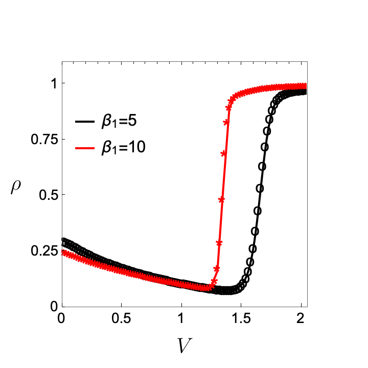
Figure 1: For the stargraph, the comparison between the exact system density $\rho$, obtained by diagonalising the evolution matrix (continuous lines), and the approximation Eqs. (19) and (22) (symbols). Circles and stars correspond to $\beta_{1}=5$ and $\beta_{1}=10$, respectively. Parameters: $N=30,F=1,E_{a}=2$ and $\beta_{2}=1$.

IV.2 General features and heat maps for finite $N$

To reduce the number of parameters, we will assume that $\beta_{2}=1$ unless specified otherwise. Furthermore, we will look at $\epsilon=0.1$ and $1$ and vary $\beta_{1}$. Figs. 2 and 3 summarize the main findings about minimal models for interacting for a small system of size $N=20$.

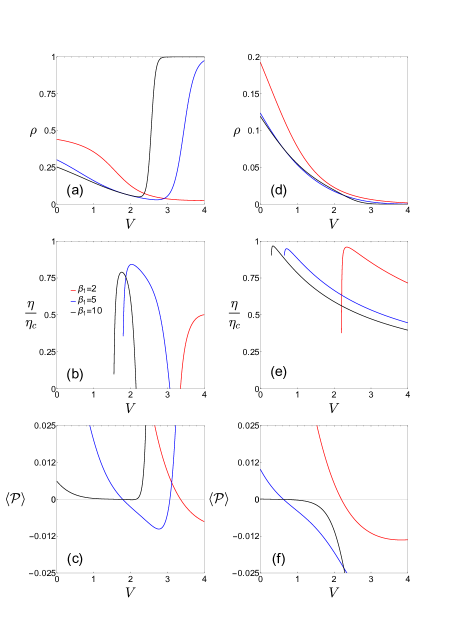
Figure 2: System density $\rho$ (top), efficiency $\eta/\eta_{c}$ (center) and power $\langle{\cal P}\rangle\equiv{\cal P}/N$ per particle (bottom) versus $V$ for the all-to-all case, for $\epsilon=0.1$ (left panels) and $\epsilon=1$ (right panels). Discontinuities in the efficiency correspond to crossovers from pump-dud and dud-engine regimes. Parameters: $F=1,E_{a}=2$ and $\beta_{2}=1$.

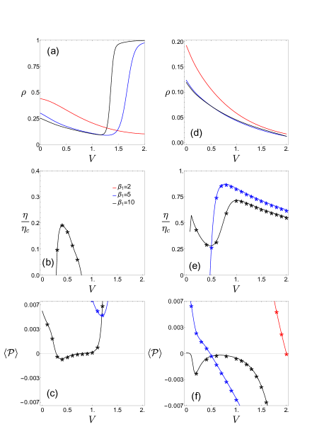
Figure 3: System density $\rho$ (top), efficiency $\eta/\eta_{c}$ (center) and power $\langle{\cal P}\rangle\equiv{\cal P}/N$ per particle (bottom) versus $V$ for the stargraph case, for $\epsilon=0.1$ (left panels) and $\epsilon=1$ (right panels). Symbols denote results from numerical simulations. Parameters: $F=1,E_{a}=2$ and $\beta_{2}=1$.

As the all-to-all, the increase of interaction strength $V$ also changes $\rho$ significantly for the stargraph and, consequently, affects the engine performance. While intermediate densities favor the system operation as a pump, their emptying when $V$ is increased changes the operation regime, from a pump to a heat engine and also increases the engine performance, whose performances are meaningfully different for $\epsilon=0.1$ (smaller) and $1$ (larger) individual $\beta_{\nu}\epsilon$’s. The maximal reachable efficiency $\eta_{ME}$ is always lower than $\eta_{c}$ for finite $N$, as expected.

Another common behavior in both cases is the fact that large $V$ favors a full occupation of the upper state when $\beta_{\nu}\epsilon$ is small (see e.g. panels $(a)$ in Figs. 2 and 3), implying that the system operates dudly when most of units are in the upper state, whose crossover from heat to dud regime is marked by a discontinuous phase transition. Conversely, the increase of $\epsilon$ marks the absence of phase transition for a broader range of $V$ and consequently not only extends the engine regime but also improves system performance. Despite closely dependent on parameters, both $\eta$ and ${\cal P}$ exhibit similar trends as $\beta_{1}$ is raised for the all to all case. Although having inferior performance than the all-to-all (at least for the chosen set of parameters), the stargraph yield some striking features for smaller $N$ (see e.g. in Figs. 3, 5 and 6), including an intermediate sets of $V$ in which both $\eta$ and ${\cal P}$ do not behave monotonously, characterized by a local and global maximum ($\eta_{MP}$) and minimum (${\cal P}_{mP}$), as can be seen in Figs. 3 $(e)-(f)$. In all cases, exact results (continuous) agree very well with numerical simulations (symbols).

A global phase-portrait is depicted in Figs. 4 and 5 for $N=20$. These results are in agreement with the aforementioned and reinforce previous findings, including larger maximum efficiencies and power for all-to-all interactions than stargraph ones for small $N$’s, but such later one presents two distinct regions (for lower and larger $V$’s) which the heat engine operates more efficiently. Similar findings are shown in Sec. .1 for ${\cal P}$’s.

In Secs. IV.3 and IV.4, remarkable aspects about both minimal structures, including the existence of a discontinuous transition for smaller individual energies as well as its suppression as $\epsilon$ increases, shall be described.

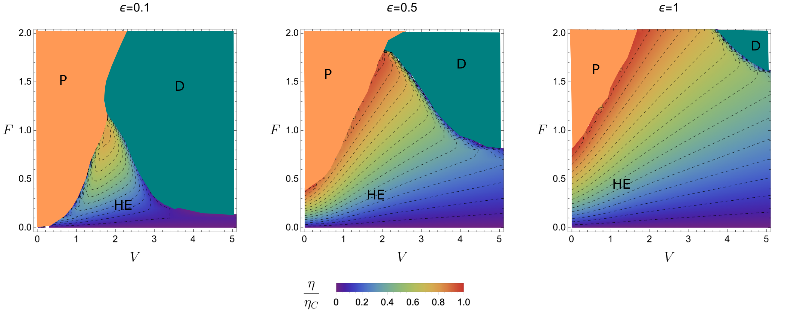
Figure 4: For the all-to-all topology, the efficiency heat maps for various choices of $\epsilon$’ as in Fig. 3. HE, P and D denote the heat engine, pump and dud regimes, respectively. Parameters: $N=20$, $E_{a}=2$, $\beta_{1}=10$, $\beta_{2}=1$.

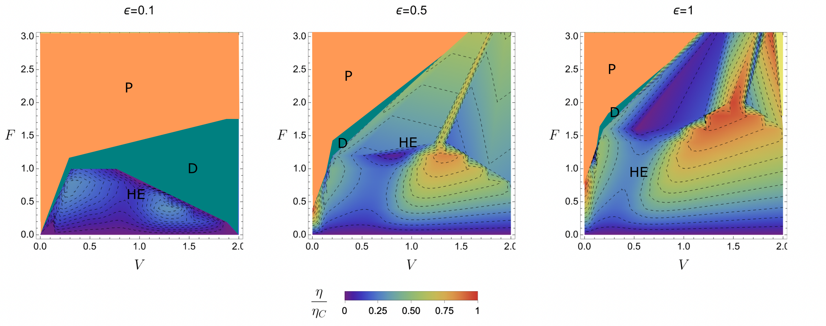
Figure 5: For the stargraph topology, the efficiency heat maps for various choices of $\epsilon$, as in Fig. 3. Parameters: $N=20$, $E_{a}=2$, $\beta_{1}=10$, $\beta_{2}=1$.

IV.3 Effect of system sizes and phase transitions

The first common aspect regarding the behavior of stargraph and all-to-all interaction structures is that the increase of interaction $V$ (for smaller values of $\beta_{\nu}\epsilon$) not only influences the system properties and the engine’s performance but also gives rise to a phase transition characterized by a full occupancy of units in the upper state as $N\rightarrow\infty$. However, the behavior of finite systems provides some clues about the classification of phase transition, as described by the finite size scaling theory Ódor (2008); Henkel (2008); Fiore and da Luz (2011); Fiore (2011); Fiore and Carneiro (2007); de Oliveira et al. (2015, 2018). In the present case, the existence of a crossing among curves for distinct (finite) system sizes $N$ reveals a discontinuous phase transition de Oliveira et al. (2015, 2018), as depicted in Fig. 6.

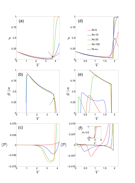
Figure 6: The effect of system size in minimal collectively models: Left and right panels depict the behavior of density (top), $\eta/\eta_{c}$ (center) and $\langle{\cal P}\rangle\equiv{\cal P}/N$ (bottom) for the all-to-all and the stargraph, respectively. Arrows indicate the discontinuous phase transitions, characterized by the crossing among curves. The inset in the right bottom panel indicates the hub density for the stargraph model. Dashed lines: Results for $N\rightarrow\infty$. Parameters: $F=1,E_{a}=2,\epsilon=0.5,\beta_{1}=10$ and $\beta_{2}=1$.

More specifically, the density curves $\rho$ strongly depend on the system size near phase-transition $V_{0}$ ($V_{0}=3.712(3)$ and $1.942(2)$ for the all-to-all and stargraph, respectively), whose intersection among curves is consistent to a density jump for $N\rightarrow\infty$. Such features are also manifested in the behavior of both $\eta$ and ${\cal P}$ (see arrows in Figs. 6), marking the coexistence between heat engine and dud regimes. The opposite scenario is verified by raising $\epsilon$, as depicted in Fig. 7 for $\epsilon=1$ for both all-to-all and stargraph topologies. Unlike the behavior of $\epsilon=0.5$, the phase transition is absent for both structures and as a consequence, the heat engine regime is broader.

We close this section by stressing that, although discontinuous phase transition have already been reported for similar systems Vroylandt et al. (2017), the existence of a phase transition in the stargraph structure is revealing and suggests that a minimal interaction structure is sufficient for introducing collective effects that are responsible for the phase transition.

IV.4 The $N\rightarrow\infty$ limit and phenomenological descriptions

A question which naturally arises concerns the system behavior in the thermodynamic limit $N\rightarrow\infty$ for both all-to-all and stargraph structures. The former case is rather simple and can be derived directly from transition rates, in which system behavior is described by a master equation with non linear transition rates. Since the all-to-all dynamics is fully characterized by the quantity $n$, the macroscopic dynamics is given by the probability of occupation $p_{1}$, corresponding to $\rho$ in the thermodynamic limit $p_{1}={\lim}_{N\rightarrow\infty}\sum_{i=1}^{N}ip^{st}(i)/N$ ($p_{0}=1-p_{1}$) Vroylandt et al. (2017); Filho et al. (2023) and described by the master equation that has the form ${\dot{p}}_{1}=\sum_{\nu=1}^{2}J^{(\nu)}_{10}$, such that:

$${\dot{p}}_{1}=\sum_{\nu=1}^{2}[\omega^{(\nu)}_{10}(1-p_{1})-\omega^{(\nu)}_{01}p_{1}],$$ (25)

where transition rates $\omega^{(\nu)}_{10}$ and $\omega^{(\nu)}_{01}$ denote the transition the lower to the higher stateand vice versa, respectively, and are listed below:

$$\omega^{(1)}_{10}=\Gamma e^{-\frac{\beta_{1}}{2}\{E_{a}+\Delta E_{10}-F\}},$$

$$\omega^{(2)}_{01}=\Gamma e^{-\frac{\beta_{2}}{2}\{E_{a}-\Delta E_{10}+F\}},$$ (26)

where $\Delta E_{10}=V(1-2p_{1})+\epsilon$. For $N\rightarrow\infty$, expressions for the power $\langle{\cal P}\rangle\equiv{\cal P}/N$ and heat per unit $\langle\dot{\mathcal{Q}}_{\nu}\rangle\equiv\langle\dot{{Q}}_{\nu}\rangle/N$ from Eqs. (11) and (12) read

$$\langle{\cal P}\rangle=F(J_{10}^{(1)}-J_{10}^{(2)})\quad{\rm and}\quad$$ (27)

$$\langle\dot{\mathcal{Q}}_{\nu}\rangle=\left(\Delta E_{10}+(-1)^{\nu}F\right)J_{10}^{(\nu)}$$ (28)

respectively. $p_{1}$ is obtained by solving Eq. (25). As shown in Sec. IV.3, small and large values of individual energy $\beta_{\nu}\epsilon$ mark different behaviors a $N$ increases, the former yielding a discontinuous phase transition. Unlike the behavior of finite $N$, the discontinuous phase transition is featured by the existence of a hysteretic branch in which the system has a bistable behavior Vroylandt et al. (2017). We shall focus on $\epsilon=1$ which describes the behavior of large $\beta_{\nu}\epsilon$’s, as depicted in Fig. 7, together with a comparison with different $N$’s. As can be seen in this figure, in both cases, maximum efficiencies $\eta_{ME}$’s (for coupling strength V=$V_{ME}$’s) and (absolute) minimum powers ${\cal P}_{mP}$’s (for coupling strength $V=V_{mP}$’s) increase as $N$ is raised and approaching to the $N\rightarrow\infty$, consistent with enhancing collective effects. However, contrasting with the power, the efficiency for smaller system sizes is larger for $V>V_{ME}$. This can be understood from the interplay between power and $\langle\dot{Q}_{2}\rangle$. For $V>V_{mP}$, the power mildly changes with $N$, whereas $\langle\dot{Q}_{2}\rangle/N$ monotonically increases with $N$. Likewise for ${V_{ME}}<V<V_{mP}$, but in this case $\langle\dot{Q}_{2}\rangle/N$ increases “faster” than $\langle{\cal P}\rangle$.

Although Eq. (25) can be solved numerically for any set of parameters, its nonlinear shape makes it impossible to obtain analytical results. However, it is possible to get some insights about the system in the heat engine regime when $p_{1}<<1$ (and $p_{0}$ is close to $1$). In this case, the terms $p_{1}$ and $p_{0}$ appearing in transition rates can be neglected and treated as $p_{0}\approx 1$, respectively, in such a way one arrives at the followingformula:

$$p_{1}\approx\frac{\omega^{(1)}_{10}+\omega^{(2)}_{10}}{\omega^{(1)}_{01}+\omega^{(2)}_{01}+\omega^{(1)}_{10}+\omega^{(2)}_{10}}.$$ (29)

By inserting transition rates from Eq. (26) into Eq. (29), we arrive at the following approximate expression for $p_{1}$:

$$\centering p_{1}\approx\frac{\mathcal{A}_{1}e^{-\frac{1}{2}\beta_{1}\left(V+\epsilon-F\right)}+\mathcal{A}_{2}e^{-\frac{1}{2}\beta_{2}\left(V+\epsilon+F\right)}}{\mathcal{A}_{1}e^{\frac{1}{2}\beta_{1}\left(V+\epsilon-F\right)}+\mathcal{A}_{2}e^{\frac{1}{2}\beta_{2}\left(V+\epsilon+F\right)}},\@add@centering$$ (30)

where $\mathcal{A}_{\nu}=e^{-\frac{\beta_{\nu}}{2}E_{a}}$. Approximate expressions for ${\cal P}$ and $\langle Q_{\nu}\rangle$’s in the heat engine are promptly obtained inserting Eq. (30) into Eqs. (27) and (28), respectively. Although they are cumbersome, they solely depend on the model parameters $\beta_{1},\beta_{2},E_{a},\epsilon,F$ and $V$. The comparison between exact and approximate results is also shown in top panels from Fig. 7 (symbols) for $\epsilon=1$, in which no phase transition yields (at least for limited $V$’s). As can be seen, the agreement is very good for $p_{1}<<1$.

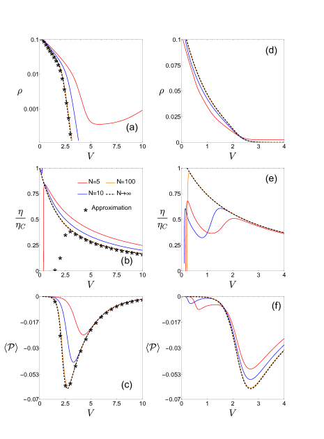
Figure 7: Depiction of system density (top), $\eta/\eta_{c}$ (center) and $\langle{\cal P}\rangle\equiv{\cal P}/N$ (bottom) for distinct system sizes and also for the $N\rightarrow\infty$ limit for all-to-all(left) and stargraph(right). The monolog plot of $\rho$ in $(a)$ has been considered in order to validate Eq.(29). Dotted lines: the phenomenological description for the all-to-all case. Parameters: $\beta_{1}=10$, $\beta_{2}=1$, $E_{a}=2$, $\epsilon=1$ and $F=1$.

The limit $N\rightarrow\infty$ for the stargraph is obtained in a similar way, but leaves and hub are treated separately. Given that Eqs. (9) and (22) present similar forms, the density of leaves $p_{1}={\lim}_{N\rightarrow\infty}\sum_{i=1}^{N-1}ip^{st}(i)/N$ also has the form of Eq. (29) and are given by

$$p_{1}=\frac{\omega^{(c,1)}_{10}+\omega^{(c,2)}_{10}}{\omega^{(c,1)}_{10}+\omega^{(c,1)}_{01}+\omega^{(c,2)}_{10}+\omega^{(c,2)}_{01}},$$ (31)

where transition rates given by

$$\omega^{(c,\nu)}_{10} = \Gamma e^{-\frac{\beta_{\nu}}{2}\left[E_{a}+\epsilon+V(1-2c)+F(-1)^{\nu}\right]},$$ (32)

$$\omega^{(c,\nu)}_{01} = \Gamma e^{-\frac{\beta_{\nu}}{2}\left[E_{a}-\epsilon-V(1-2c)-F(-1)^{\nu}\right]}.$$ (33)

Since $p_{1}$ is dependent on the hub occupation, it is worth investigating its behavior when $N\rightarrow\infty$. From Eq. (19), $p^{st}(1|n)\rightarrow 0$ and $1$ for $n<N/2$ and $n>N/2$, respectively, as $N\rightarrow\infty$. Also, $p_{h}=\sum_{n=0}^{N-1}p^{st}(1|n)p^{st}(n)/N\rightarrow 0$ and $1$ when $p_{1}$ is small and large, respectively. From Eqs. (23) and (IV.1), expressions for the power $\langle{\cal P}\rangle\equiv{\cal P}/N$ and heat $\langle\dot{\mathcal{Q}}_{\nu}\rangle\equiv\langle\dot{{Q}}_{\nu}\rangle/N$ are obtained by noting that the hub contribution vanishes as limit $N\rightarrow\infty$ and hence they read

$$\langle{\cal P}\rangle=F\left[(\pi_{10}^{(1)}-\pi_{10}^{(2)})(1-p_{1})-(\pi_{01}^{(1)}-\pi_{01}^{(2)})p_{1}\right],$$ (34)

and

$$\centering\left\langle\dot{\mathcal{Q}}_{\nu}\right\rangle\@add@centering = \left[\epsilon+V(1-2c)+(-1)^{\nu}F\right]\left[\pi_{10}^{(\nu)}-(\pi_{10}^{(\nu)}+\pi_{01}^{(\nu)})p_{1}\right],$$ (35)

respectively, where $\pi_{10}^{(\nu)}=\omega^{(0,\nu)}_{10}$ and $\pi_{10}^{(\nu)}=\omega^{(1,\nu)}_{10}$ provided $p_{h}=0$ and $1$, respectively. Efficiency $\eta$ is straightforwardly evaluated using the above equations

$$\eta=-\frac{F\left[(\pi_{10}^{(1)}-\pi_{10}^{(2)})(1-p_{1})-(\pi_{01}^{(1)}-\pi_{01}^{(2)})p_{1}\right]}{\left[\epsilon+V(1-2c)+F\right]\left[\pi_{10}^{(2)}-(\pi_{10}^{(2)}+\pi_{01}^{(2)})p_{1}\right]}.$$ (36)

We pause again to make a few comments about Eq. (36). For small values of $\beta_{\nu}\epsilon$, in which a discontinuous phase transition yields at $V_{0}$, $p_{h}$ jumps from $0$ to $1$ for $V<V_{0-}$ and $V>V_{0+}$, respectively, and $p_{h}=1/2$ precisely at $V=V_{0}$. Second, from the hub behavior, it follows that $p_{1}$ jumps from $p_{1-}$ to $p_{1+}$, where $p_{1-}$($p_{1+}$) are obtained from Eq. (31) evaluated at $c=0$ (for $V\rightarrow V_{0-}$) and $c=1$ (for $V\rightarrow V_{0+}$), respectively. Third, the order-parameter jump is also followed by discontinuities in the behavior of thermodynamic quantities, such as $\langle{\cal P}\rangle$ and $\eta$. They are evaluated from Eqs. (34) and (36) at $c=0$ and $V=V_{0-}$ to $c=1$ and $V=V_{0+}$, respectively. Fourth and last, large $\beta_{\nu}\epsilon$’s mark no phase transitions for limited values of $V$ and hence the power and efficiency are evaluated at $c=0$ (since $p_{h}=0$). All above findings, together the reliability of Eqs. (31), (34) and (36) for small and large values of $\beta_{\nu}\epsilon$, are depicted in bottom panels from Figs. 6 and 7 for $\epsilon=0.5$ and $1$, respectively. As for the all-to-all, thermodynamics quantities for finite $N$ approach to the $N\rightarrow\infty$ limit as $N$ is increased.

We close this section by drawing a comparison between all-to-all and stargraph performances in the heat engine regime for the same set of parameters in Figs. 6 and 7. While the former structure is more efficient, stargraph ones present larger power outputs.

V Beyond the minimal models: Homogeneous and Heterogeneous topologies

In this section, we will go beyond the minimal models and look at both homogeneous and heterogeneous structures. Unlike minimal models, it is not possible to obtain analytical expressions and our analysis will focus on numerical simulations using the Gillespie method Gillespie (1977). Due to the existence of several parameters ($\beta_{1},\beta_{2},F,\epsilon,V$ and $E_{a}$), we shall center our analysis on $F=1,\beta_{1}=5$ and $\beta_{2}=1$, in which results minimal models predict a marked engine regime as $V$ is varied. Fig. 8 and 9 depict some results for homogeneous and heterogeneous structures, respectively.

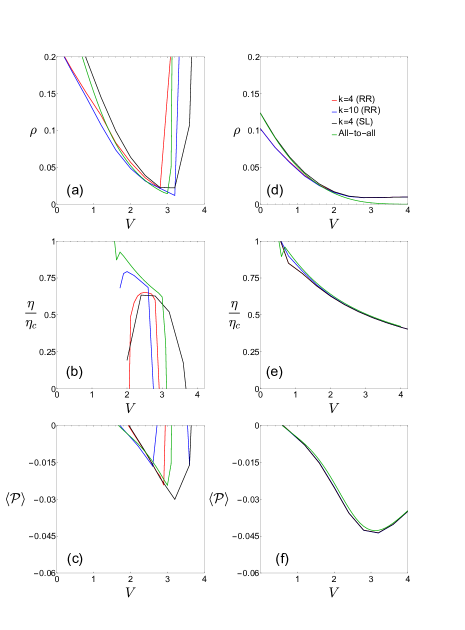
Figure 8: Results for homogeneous topologies with distinct connectivities $k$’s. Depiction of density $\rho$ (top), efficiency $\eta/\eta_{c}$ (center) and $\langle{\cal P}\rangle\equiv{\cal P}/N$ (bottom) versus coupling for $\epsilon=0.1$ (left) and $1$ (right). Symbols RR and SL denote square-lattice and random-regular topologies, respectively. Parameters: $\beta_{1}=5,\beta_{2}=1,F=1$ and $E_{a}=2$.

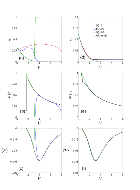
Figure 9: Results for heterogeneous topologies with distinct mean connectivities $\langle k\rangle$. Depiction of $\rho$ (top), efficiency $\eta/\eta_{c}$ (center) and $\langle{\cal P}\rangle\equiv{\cal P}/N$ (bottom) versus coupling for $\epsilon=0.1$ (left) and $1$ (right). Parameters: $\beta_{1}=5,\beta_{2}=1,F=1$ and $E_{a}=2$.

Starting our analysis for $\epsilon=0.1$ (top panels) and homogeneous arrangements, we see [Fig. 8(a) and (c)] that the system performance increases by increasing the connectivity $k$ and there are small differences between regular and random-regular arrangements. Unlike the homogeneous case, differences between $\langle k\rangle$’s are particularly clear for heterogeneous structures, where the heat engine is absent for $\langle k\rangle=4$. In this case, the system only operates as a pump, similarly to the stargraph, see e.g. Fig. 3 for $N=20$. On the other hand, the heat engine is present for $\langle k\rangle=10$ and $40$. A possible explanation is that the former and latter cases are closer to the stargraph and the all to all structures, respectively.

The results for $\epsilon=1$ (bottom panels) are remarkably different. We see that the heat engine regime becomes much larger in terms of $V$ (with $\rho$ monotonously decreasing as $V$ goes up). Furthermore, one can see that the influence of the lattice topology and neighborhood becomes negligible and the results become very similar to those of the all-to-all topology, revealing that the role of topology is not so important for larger $\beta_{\nu}\epsilon$’s.

VI conclusions

In this paper, we studied the role of topology of interactions on the performance of thermal engines. We investigated four distinct topologies for a simple setup composed of interacting unicyclic machines, each one allowed to be in two states: all-to-all, stargraph, homogeneous and heterogeneous structures. Different findings can be extracted from the present study. Interestingly, the interplay among parameters (individual $\beta_{\nu}\epsilon$, interaction energies $V$ and temperatures) provides two opposite scenarios, in which the role of topology is important and less important respectively, depending on whether $\beta_{\nu}\epsilon$ is small or large. The former case not only shows a discontinuous phase transition as the interaction is raised, but also how the increase of neighborhood (both homogeneous and heterogeneous) increases the efficiency but in contrast its power is inferior. Since a majority fraction of are empty in the latter case, the topology of interactions plays no major role.

As a final comment, we mention some ideas for future research. It might be interesting to study the the full statistics of power and efficiency in different lattice topologies, in order to tackle the influences of fluctuations. Also, it might be interesting to compare the performance of different engine projections, such as those composed interacting units placed in contact with only one thermal bath in instead of two, in order to compare the system’s performances as well a the influence of lattice topology in those cases. Finally, it shall be interesting to investigate the inclusion of interactions between units in the same sate (as considered in Ref. Prech et al. (2023)) as its competition with interactions given by Eq. (3).

VII Acknowledgments

We acknowledge the financial support from Brazilian agencies CNPq and FAPESP under grants 2021/03372-2, 2021/12551-8 and 2023/00096-0.

Appendix

.1 Power-output heat maps for the minimal models

In this appendix, we show in Figs. A1 and A2 the heat maps for the power output for both all-to-all and stargraph cases for $N=20$ for the same parameters from figs. 4 and 5.

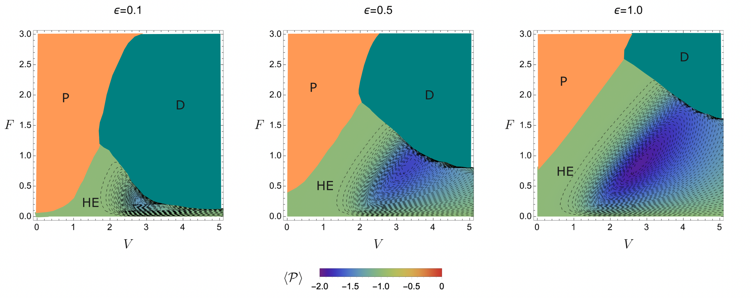
Figure A1: For the all-to-all case, $\left\langle\mathcal{P}\right\rangle$ heat maps for the same $\epsilon$ in Fig. 3. Parameters: $N=20$, $E_{a}=2$, $\beta_{1}=10$, $\beta_{2}=1$.

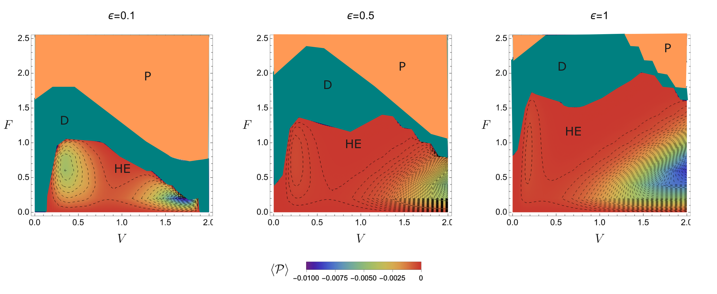
Figure A2: Heat maps for the power of the stargraph model for different values of $\epsilon$.Parameters: $N=20$, $E_{a}=2$, $\beta_{1}=10$, $\beta_{2}=1$

Finally, Fig. A3 draws a global comparison among all structures for $\epsilon=1$. As can be seen, there is small difference among structures, conferring some somewhat superior efficiencies for large connectivities.

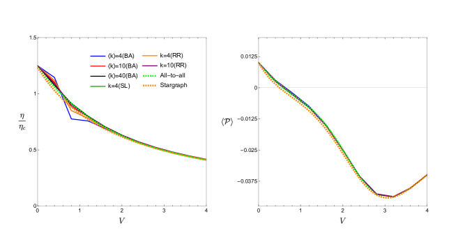
Figure A3: Depiction of $\eta/\eta_{c}$ and $\left\langle\mathcal{P}\right\rangle$ for all the topologies. Symbols RR, SL and BA denote square-lattice, random-regular and heterogeneous (Barabasi-Albert) topologies, respectively.Parameters:$\beta_{1}=5,\beta_{2}=1,E_{a}=2,\epsilon=1$ and $F=1$.

References

- Carnot (1978) S. Carnot, Réflexions sur la puissance motrice du feu, 26 (Vrin, 1978).
- Curzon and Ahlborn (1975) F. Curzon and B. Ahlborn, American Journal of Physics 43, 22 (1975).
- Seifert (2012) U. Seifert, Reports on progress in physics 75, 126001 (2012).
- Van den Broeck and Esposito (2015) C. Van den Broeck and M. Esposito, Physica A: Statistical Mechanics and its Applications 418, 6 (2015).
- Verley et al. (2014) G. Verley, M. Esposito, T. Willaert, and C. Van den Broeck, Nature Communications 5, 4721 (2014).
- Schmiedl and Seifert (2007) T. Schmiedl and U. Seifert, EPL (Europhysics Letters) 81, 20003 (2007).
- Cleuren et al. (2015) B. Cleuren, B. Rutten, and C. Van den Broeck, The European Physical Journal Special Topics 224, 879 (2015).
- Van den Broeck (2005) C. Van den Broeck, Physical Review Letters 95, 190602 (2005).
- Esposito et al. (2010) M. Esposito, R. Kawai, K. Lindenberg, and C. Van den Broeck, Physical Review E 81, 041106 (2010).
- Seifert (2011) U. Seifert, Physical Review Letters 106, 020601 (2011).
- Izumida and Okuda (2012) Y. Izumida and K. Okuda, Europhysics Letters 97, 10004 (2012).
- Golubeva and Imparato (2012) N. Golubeva and A. Imparato, Physical Review Letters 109, 190602 (2012).
- Holubec (2014) V. Holubec, Journal of Statistical Mechanics: Theory and Experiment 2014, P05022 (2014).
- Bauer et al. (2016) M. Bauer, K. Brandner, and U. Seifert, Physical Review E 93, 042112 (2016).
- Proesmans et al. (2016a) K. Proesmans, B. Cleuren, and C. Van den Broeck, Physical review letters 116, 220601 (2016a).
- Tu (2008) Z. Tu, Journal of Physics A: Mathematical and Theoretical 41, 312003 (2008).
- Ciliberto (2017) S. Ciliberto, Physical Review X 7, 021051 (2017).
- Bonança (2019) M. V. S. Bonança, Journal of Statistical Mechanics: Theory and Experiment 2019, 123203 (2019).
- Mamede et al. (2022) I. N. Mamede, P. E. Harunari, B. A. N. Akasaki, K. Proesmans, and C. E. Fiore, Phys. Rev. E 105, 024106 (2022).
- Proesmans et al. (2016b) K. Proesmans, B. Cleuren, and C. Van den Broeck, Physical review letters 116, 220601 (2016b).
- Noa et al. (2021) C. E. F. Noa, A. L. L. Stable, W. G. C. Oropesa, A. Rosas, and C. E. Fiore, Phys. Rev. Research 3, 043152 (2021).
- (22) P. E. Harunari, F. S. Filho, C. E. Fiore, and A. Rosas, arXiv:2012.09296 .
- Guéry-Odelin et al. (2019) D. Guéry-Odelin, A. Ruschhaupt, A. Kiely, E. Torrontegui, S. Martínez-Garaot, and J. G. Muga, Rev. Mod. Phys. 91, 045001 (2019).
- Deffner and Bonança (2020) S. Deffner and M. V. Bonança, EPL (Europhysics Letters) 131, 20001 (2020).
- Pancotti et al. (2020) N. Pancotti, M. Scandi, M. T. Mitchison, and M. Perarnau-Llobet, Physical Review X 10, 031015 (2020).
- Zhao et al. (2022) X.-H. Zhao, Z.-N. Gong, and Z. C. Tu, “Microscopic low-dissipation heat engine via shortcuts to adiabaticity and shortcuts to isothermality,” (2022).
- Hooyberghs et al. (2013) H. Hooyberghs, B. Cleuren, A. Salazar, J. O. Indekeu, and C. Van den Broeck, The Journal of chemical physics 139 (2013).
- Campisi and Fazio (2016) M. Campisi and R. Fazio, Nature communications 7, 1 (2016).
- Yeomans (1992) J. M. Yeomans, Statistical mechanics of phase transitions (Clarendon Press, 1992).
- Torres et al. (2005) J. Torres, L. Bonilla, C. J. P. Vicente, F. Ritort, R. Spigler, et al., Reviews of Modern Physics 77, 137 (2005).
- Tönjes et al. (2021) R. Tönjes, C. E. Fiore, and T. Pereira, Nature Communications 12, 1 (2021).
- Bonifazi et al. (2009) P. Bonifazi, M. Goldin, M. A. Picardo, I. Jorquera, A. Cattani, G. Bianconi, A. Represa, Y. Ben-Ari, and R. Cossart, Science 326, 1419 (2009).
- Schneidman et al. (2006) E. Schneidman, M. J. Berry, R. Segev, and W. Bialek, Nature 440, 1007 (2006).
- Buzsáki and Mizuseki (2014) G. Buzsáki and K. Mizuseki, Nature Reviews Neuroscience 15, 264 (2014).
- Gal et al. (2017) E. Gal, M. London, A. Globerson, S. Ramaswamy, M. W. Reimann, E. Muller, H. Markram, and I. Segev, Nature neuroscience 20, 1004 (2017).
- Rapoport (1970) S. I. Rapoport, Biophysical Journal 10, 246 (1970).
- Gnesotto et al. (2018) F. S. Gnesotto, F. Mura, J. Gladrow, and C. P. Broedersz, Reports on Progress in Physics 81, 066601 (2018).
- Lynn et al. (2021) C. W. Lynn, E. J. Cornblath, L. Papadopoulos, M. A. Bertolero, and D. S. Bassett, Proceedings of the National Academy of Sciences 118, e2109889118 (2021).
- Smith and Schuster (2019) P. Smith and M. Schuster, Current Biology 29, R442 (2019).
- Mukherjee and Divakaran (2021) V. Mukherjee and U. Divakaran, Journal of Physics: Condensed Matter 33, 454001 (2021).
- Niedenzu and Kurizki (2018) W. Niedenzu and G. Kurizki, New Journal of Physics 20, 113038 (2018).
- Kurizki et al. (2015) G. Kurizki, P. Bertet, Y. Kubo, K. Mølmer, D. Petrosyan, P. Rabl, and J. Schmiedmayer, Proceedings of the National Academy of Sciences 112, 3866 (2015).
- Lee et al. (2022) Y. Lee, E. Bersin, A. Dahlberg, S. Wehner, and D. Englund, npj Quantum Information 8, 1 (2022).
- Mukherjee et al. (2020) V. Mukherjee, U. Divakaran, A. del Campo, et al., Physical Review Research 2, 043247 (2020).
- Halpern et al. (2019) N. Y. Halpern, C. D. White, S. Gopalakrishnan, and G. Refael, Physical Review B 99, 024203 (2019).
- Kim et al. (2022) J. Kim, S.-h. Oh, D. Yang, J. Kim, M. Lee, and K. An, Nature Photonics 16, 707 (2022).
- Kolisnyk and Schaller (2023) D. Kolisnyk and G. Schaller, Phys. Rev. Appl. 19, 034023 (2023).
- Latune et al. (2019) C. L. Latune, I. Sinayskiy, and F. Petruccione, Phys. Rev. Res. 1, 033192 (2019).
- Chen et al. (2019) Y. Chen, G. Watanabe, Y. Yu, X. Guan, and A. del Campo, “An interaction-driven many-particle quantum heat engine and its universal behavior, npj quant,” (2019).
- Fogedby and Imparato (2017) H. C. Fogedby and A. Imparato, EPL (Europhysics Letters) 119, 50007 (2017).
- Imparato (2021) A. Imparato, Journal of Statistical Mechanics: Theory and Experiment 2021, 013214 (2021).
- Suñé and Imparato (2019) M. Suñé and A. Imparato, Phys. Rev. Lett. 123, 070601 (2019).
- Vroylandt et al. (2017) H. Vroylandt, M. Esposito, and G. Verley, EPL (Europhysics Letters) 120, 30009 (2017).
- Vroylandt et al. (2020) H. Vroylandt, M. Esposito, and G. Verley, Physical Review Letters 124, 250603 (2020).
- Herpich et al. (2018) T. Herpich, J. Thingna, and M. Esposito, Phys. Rev. X 8, 031056 (2018).
- Herpich and Esposito (2019) T. Herpich and M. Esposito, Phys. Rev. E 99, 022135 (2019).
- Filho et al. (2023) F. S. Filho, G. A. Forão, D. M. Busiello, B. Cleuren, and C. E. Fiore, arXiv preprint arXiv:2301.06591 (2023).
- Cleuren and Van den Broeck (2001) B. Cleuren and C. Van den Broeck, EPL (Europhysics Letters) 54, 1 (2001).
- Prech et al. (2023) K. Prech, P. Johansson, E. Nyholm, G. T. Landi, C. Verdozzi, P. Samuelsson, and P. P. Potts, Phys. Rev. Res. 5, 023155 (2023).
- Cuetara and Esposito (2015) G. B. Cuetara and M. Esposito, New Journal of Physics 17, 095005 (2015).
- Liepelt and Lipowsky (2007) S. Liepelt and R. Lipowsky, Phys. Rev. Lett. 98, 258102 (2007).
- Liepelt and Lipowsky (2009) S. Liepelt and R. Lipowsky, Phys. Rev. E 79, 011917 (2009).
- Berton et al. (2020) C. Berton, D. M. Busiello, S. Zamuner, E. Solari, R. Scopelliti, F. Fadaei-Tirani, K. Severin, and C. Pezzato, Chemical Science 11, 8457 (2020).
- De Los Rios and Barducci (2014) P. De Los Rios and A. Barducci, Elife 3, e02218 (2014).
- Bollobás (1980) B. Bollobás, European Journal of Combinatorics 1, 311 (1980).
- Barabási and Albert (1999) A.-L. Barabási and R. Albert, science 286, 509 (1999).
- Barrat et al. (2008) A. Barrat, M. Barthelemy, and A. Vespignani, Dynamical processes on complex networks (Cambridge university press, 2008).
- Vlasov et al. (2015) V. Vlasov, Y. Zou, and T. Pereira, Phys. Rev. E 92, 012904 (2015).
- Ódor (2008) G. Ódor, Universality in nonequilibrium lattice systems: theoretical foundations (World Scientific, 2008).
- Henkel (2008) M. Henkel, Non-equilibrium phase transitions (Springer, 2008).
- Fiore and da Luz (2011) C. E. Fiore and M. G. E. da Luz, Phys. Rev. Lett. 107, 230601 (2011).
- Fiore (2011) C. E. Fiore, The Journal of chemical physics 135 (2011).
- Fiore and Carneiro (2007) C. E. Fiore and C. E. I. Carneiro, Phys. Rev. E 76, 021118 (2007).
- de Oliveira et al. (2015) M. M. de Oliveira, M. G. E. da Luz, and C. E. Fiore, Phys. Rev. E 92, 062126 (2015).
- de Oliveira et al. (2018) M. M. de Oliveira, M. G. E. da Luz, and C. E. Fiore, Phys. Rev. E 97, 060101 (2018).
- Gillespie (1977) D. T. Gillespie, The journal of physical chemistry 81, 2340 (1977).