On the Calibration of Uncertainty Estimation in LiDAR-based Semantic Segmentation

Abstract

The confidence calibration of deep learning-based perception models plays a crucial role in their reliability. Especially in the context of autonomous driving, downstream tasks like prediction and planning depend on accurate confidence estimates. In the point-wise multiclass classification tasks of sematic segmentation the model naturally has to deal with heavy class imbalances. Due to their underrepresentation, the confidence calibration of classes with smaller instances is challenging but essential, especially for safety reasons. We propose a metric to measure the confidence calibration quality of a semantic segmentation model with respect to individual classes. It utilizes the computation of sparsification curves based on uncertainty estimates. With the help of this classification calibration metric, uncertainty estimation methods can be evaluated with respect to their confidence calibration of any given classes. We furthermore suggest a method to automatically find label problems using this metric to improve the quality of hand- or auto-annotated datasets.

I Introduction

Environment perception is a prerequisite for most autonomous driving systems. It allows the vehicle to detect and understand the behavior of other participants and enables it to adapt its own behavior accordingly. Deep learning methods took performance in evironment perception to a new level by constructing models which can evaluate large amounts of data. These data are gathered by various sensors with different modalities, such as cameras, radar and LiDAR sensors. In the past few years, the LiDAR sensor gained relevance in the context of environment perception for autonomous vehicles due to the added value of highly precise depth information.

Besides perception tasks like object detection and tracking, semantic segmentation plays a crucial role in scene understanding for autonomous vehicles. The task of a semantic segmentation model is to classify every measurement individually to obtain a detailed representation of the environment including e.g. drivable space, vulnerable road users or non-movable objects. The point-wise multi-class semantic segmentation of semi-dense LiDAR data based on deep learning has been studied thoroughly during the last years [1], [2]. Despite major advances in this field, the task of semantic segmentation comes with the challenge of handling severely imbalanced data [3]. This is due to the natural distribution of spaces and objects, i.e. in a traffic scene there always will be significantly more measurements of the road or buildings than of persons or bicyclists.

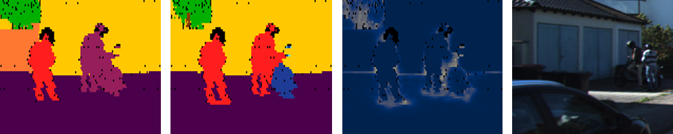
semantic segmentation: vegetation trunk building fence person motorcyclist motorcycle bicycle
uncertainty estimation: low, high

Figure 1: Example of the semantic segmentation of a person and a motorcyclist captured in a projected LiDAR-scan. From left to right: ground-truth label, model prediction, estimated predictive uncertainty. In this case, the model does not predict the label motorcyclist but instead both person and motorcycle with a high confidence. This is technically not incorrect and renders the labeling questionable in this case.

Althought the current state-of-the-art methods reach a high performance, a deeper understanding of underrepresented classes within the model weights is still challenging. In addition, although deep learning is a powerful tool and successful at generalizing within a known domain, it is prone to failure in situations they have rarely encountered before. Uncertainty estimation can help to address both of these challenges since it allows the model to to detect its own boundaries by providing confidence estimations with their predictions or classifications and it increases the transparency of the classification. Furthermore, in the context of LiDAR-based computer vision it is especially important to harvest all available information, due to the natural sparsity of the data. Uncertainty estimation helps to gather additional insights of the learning process, especially in the case of imbalanced data.

Downstream tasks rely on well calibrated confidence estimates, which match the actual performance. This allows the sensor fusion or behavior planning to reliably interpret the models abilities. In the past, the softmax probabilities were sometimes interpreted as the model confidence, which leads to overconfident estimates [4]. This indicates the need of alternative uncertainty estimation techniques as well as for suitable evaluation metrics to assess their performance.

There are a number of well established methods to estimate uncertainty in deep learning models [5], [6], [7], [8]. These approaches describe different takes on measuring data and model uncertainty respectively, indicating that the exact definition and measurement of the different uncertainty types is still an ongoing research topic [9].

To make a step towards understanding the confidence calibration of underrepresented classes in semantic segmentation tasks, we elaborate in this paper how the different uncertainty estimation methods behave under different training conditions. For that, we propose a metric to appropriately capture the confidence calibration of a semantic segmentation model and demonstrate its relevance with a series of experiments. Our proposed metric can furthermore be used to uncover questionable labels (compare Fig. 1) and paves the path for a qualitative inspection of potentially insufficient label representation.

The contributions of this paper can be concluded as:

• a flexible metric to assess the uncertainty estimation abilities of semantic segmentation models

• an evaluation of underrepresented classes in the context of LiDAR-based semantic segmentation

• a novel method to detect label problems based on calibrated deep learning models

II Related Work

The following chapter introduces existing literature related to the uncertainty estimation and its assessment in classification tasks like semantic segmentation.

II-A Semantic Segmentation of LiDAR point clouds

In the last years, various approaches on the semantic segmentation of point clouds have been proposed. Some operate in 3D space by utilizing voxels [10], [11] or unordered point clouds [12], [13], [14]. Other approaches project the point cloud into the 2D space in order use Convolutional Neural Networks for the semantic segmentation of the range view [15], [16], [17], [18].

Class imbalance is a problem which needs to be adressed in semantic segmentation. The well-established mean Intersection over Union (IoU) evaluation metric accounts for this issue and ensures that underrepresented classes are taken into account appropriately. The metric is widely used to assess the performance of a semantic segmentation model. Common ways to deal with that imbalance is to weight the loss function in favor of underrepresented classes [19], [15] or to construct an architecture which is able to overcome the issues imposed by smaller instances [1], [20], [21].

II-B Uncertainty Estimation in Classification Tasks

Generally speaking, there are two different kinds of uncertainty: the epistemic (model) uncertainty and the aleatoric (data) uncertainty [22]. The model uncertainty reflects the uncertainty about the model’s own learned parameters, which is due to lack of data, underrepresented effects or hidden information. The data uncertainty reflects the statistical uncertainty, which is due to noise inherent in all processes and effects. Both uncertainties combined compose the overall predictive uncertainty.

In the past years, several approaches on estimating the different uncertainty types emerged. Two popular well-established ones are Monte-Carlo Dropout (MCD) [23], [24], [25] and deep ensembles [6] [26], [27]. Both followed the idea of Bayesian deep learning and proposed methods which allow the models to infer probability distributions over the available classes. Thus, the model approximates the true posterior of the data distribution. Yarin Gal [5] stated that the model uncertainty then can be extracted from the Monte-Carlo samples by calculating the Mutual Information between the prediction and the model parameters posterior. The predictive uncertainty is indicated by the entropy over all classes.

Complementary to that, Kendall et al. [7] introduced a technique to model uncertainty estimation during training by sampling from the logits before applying the softmax function for classification. Thereby they demonstrated that the data uncertainty can be learned directly from the input, since it can be seen as a function of the data itself. This helps the model to measure and deal with data uncertainty by introducing a certain robustness into the classification.

II-C Evaluation of Uncertainty Estimations

Guo et al. [4] proposed the Expected Calibration Error (ECE) to assess the confidence calibration of a given neural network. It is defined as the expectation between the confidence and the accuracy of the model and is calculated by binning the confidence values, computing the according accuracies and taking the weighted average of the difference between the accuracy and the confidence. While this works well for tasks which actually use the accuracy as a performance metric, this approach tends to overestimate the performance for underrepresented classes [1]. The authors of [28] adapt this approach to multiclass settings, which in theory make it possible to calculate this metric for semantic segmentation tasks and weighting out the class-imbalances in the final score. Nevertheless, the previously described problem of an overestimated performance still persists.

Mukhoti et al. [29] suggested a metric to capture particular parts of the confidence calibration abilities of a semantic segmentation model. Their developed technique divides each frame into single patches, from which a confusion matrix is constructed. It contains the number of patches which are accurate and certain, accurate and uncertain, inaccurate and certain and inaccuracte and uncertain. The conditional probabilities $p(\text{accurate}|\text{certain})$, $p(\text{uncertain}|\text{inaccurate})$ and their combination Patch Accuracy vs. Patch Uncertainty (PAvPU) can then be calculated. These metrics are able to catch two properties:

• accuracy in case of confident predictions

• uncertainty in case of inaccurate predictions

Nevertheless, with respect to subsequent algorithms which rely on well calibrated outputs of a semantic segmentation model, this should be extended to:

• confidence in case of accurate predictions

Ideally, if it is possible to train the model well enough to reduce the epistemic uncertainty as far as possible so that e.g. the entropy only reflects the actual data uncertainty, a confidence calibration evaluation metric should also be able to capture this effect. Our proposed method has this desired property.

[30] proposes a confidence calibration metric for optical flow models. It is derived from Sparsification Plots, which have previously been used to evaluate uncertainty estimates. Through its point-wise nature it can easily be adapted to other point-wise perception tasks, like semantic segmentation. The authors of [31] have used it in combination with the Brier Score to determine the confidence calibration performance of semantic segmentation models. Yet, the inherent problem with the Brier Score is that it punishes deviations from the one-hot encoding, which contradicts the aim to combat overconfidence in classification models.

III Methods

The trainings presented in the following section were conducted on the training sequences of SemanticKITTI dataset [32], projected into the 2D sensor view representation [33].

III-A Semantic Segmentation Model and Training

To train a semantic segmentation model, a simplified version of the SalsaNext architecture is used [34]. It should be noted here that any semantic segmentation backbone will work in this context, especially those which come with an improved performance on imbalanced data [35].

To evaluate different training strategies, we trained our model once with the uncertainty-aware loss function for classification tasks as proposed in [7] and once we extended it to a weighted cross-entropy loss function to account for class imbalances [19]. The weights for each class are calculated according to their percentage of points $f_{c}$ compared to the total points:

$$weight_{c}=\frac{1}{\text{log}(1.02+f_{c})}$$ (1)

Following this equation (taken from [19]), underrepresented classes like motorcyclist receive higher weights than well represented classes, e.g road. For further analysis on the distribution of data-points and -labels in the SemanticKITTI dataset, see [36].

III-B Uncertainty Estimation Technique

To capture the data and the model uncertainty, both the MCD [5] (30 samples) and logit sampling (10 samples) [7] are used. In sum three uncertainty estimation methods are evaluated:

• learned aleatoric uncertainty (cf. Equation 2)

• MCD-based model uncertainty $\mathbb{I}$  (cf. Equation 4)

• MCD-based predictive uncertainty $\mathbb{H}$  (cf. Equation 3)

The aleatoric uncertainty estimation is directly incorporated into the training process by implementing a mean and standard deviation for every class instead of one single logit score:

$$\begin{split}x_{i,s}&=f_{i}^{w}+\sigma_{i}^{w}\epsilon_{t},\quad\epsilon_{s}\sim\mathcal{N}(0,I)\\ Loss_{x}&=\sum_{i}\text{log}\frac{1}{S}\sum_{s}\exp(x_{i,s,c}-\text{log}\sum_{c^{\prime}}\exp x_{i,s,c^{\prime}})\end{split}$$ (2)

with $i$ denoting the data points, $S$ the logit samples and $c$ the classes. The logit vector $x_{i},s$ is sampled from a Gaussian distribution defined through the models outputs $f_{i}^{w}$ and $\sigma_{i}^{w}$ given the current mode weights $w$ and input frame $x\in D_{train}$. The model samples 10 times from these Gaussian distributions and then outputs the class with the highest mean softmax score. This softmax probability is proven to be more calibrated than the regular softmax [7].

For the MCD process the model is trained with dropout. At test time, multiple forward passes are conducted with dropout enabled, which imitates approximating the posterior over the model weights. The Shannon Entropy ($\mathbb{H}$) over the class scores then denotes the predictive uncertainty:

$$\mathbb{H}[y|x,D_{train}]=\\ -\sum_{c}\left(\frac{1}{T}\sum_{t}p(y=c|x,w_{t})\right)\text{log}\left(\frac{1}{T}\sum_{t}p(y=c|x,w_{t})\right)$$ (3)

with $c$ ranging over all classes and $p(y=c|x,w_{t})$ being the softmax probability of input $x$ being in class $c$ given the current set of model weights $w_{t}$. $T$ denotes the number of MCD samples. The Mutual Information ($\mathbb{I}$) between this posterior and the predictive (softmax) distribution isolates the model uncertainty. It is calculated as follows:

$$\mathbb{I}[y,w|x,D_{train}]=\mathbb{H}[y|x,D_{train}]\\ +\frac{1}{T}\sum_{c,t}p(y=c|x,w_{t})\text{log}p(y=c|x,w_{t})$$ (4)

Both formulas to approximate $\mathbb{H}$ and $\mathbb{I}$ are based on [29]. To convert these two uncertainty metrics into interpretable probabilities in terms of confidence, we normalized them with their respective theoretical maximum. This is only done for visualization purposes and to achieve comparable estimates.

III-C Confidence Calibration Evaluation Metric

The design of a novel metric to assess a the uncertainty estimation performance of a semantic segmentation model is driven by the need to have a metric which fully captures all aspects of the confidence calibration. Ideally, a well calibrated model is able to predict high uncertainties when it’s predictions are inaccurate and low uncertainties when they are accurate, and vice versa.

This can be explained with an example: usually, the class person is not well represented in large datasets for the semantic segmentation task, because in traffic situations there are less measurements on people than on e.g. roads or buildings. Furthermore, under natural circumstances the human species has a broad variety of outward appearances and humans can find themselves in plentiful different situations (contrary to cars which have a somewhat predefined appearance and a very restricted set of situations in which they can appear). Now if a model correctly predicts the presence of a person, it is not helpful when it always outputs a high predictive uncertainty because the class person was not well represented within its training. The confidence outputs of every class, no matter how well it is represented in the data, should still be meaningful, not only in terms of incorrect but also in terms of correct classifications.

The metric we propose is based on the idea of the Area Under the Sparsification Error Curve (AUSE) [30]. Contrary to the ECE, which is restricted to measure the expected performance in terms of accuracy, this metric is directly applicable to any given task and thus any appropriate performance metric. By allowing a per-class evaluation, its user is able to catch more systematic uncertainty-related phenomena instead of only local relations. It has been used based on the Brier Score [31], which is a proper scoring rule for evaluating probabilistic predictions. Yet, we avoid using the Brier Score as it indirectly encourages overconfident predictions by evaluating the deviation from the one-hot encoding. Instead, we suggest using the mIoU directly, which is the common metric to evaluate semantic segmentation models.

The idea of sparsification plots is to evaluate the pointwise uncertainty estimation by creating a ranking of the uncertainty values. The pixels with the highest uncertainty are then gradually removed and the performance (i.e. the mIoU for semantic segmentation) is evaluated in the process. If the uncertainty measure actually reflects the true performance (which it should), the mIoU should monotonically increase. Ilg et al. [30] furthermore suggest a normalization based on the best possible ranking according to the ground truth labels to remove the dependence on the model performance. They refer to it as the oracle curve, which allows a fair comparison between the different classes. The difference between the sparsification and the oracle curve is called Sparsification Error. Finally, the AUSE is defined as the area under the resulting curve. The closer the sparsification curve is to the ground-truth-based oracle curve, the smaller are the AUSE values and the better is the respective confidence calibration.

We want to emphasize that through the normalization with the oracle, the AUSE isolates the calibration from the model’s classification performance. In some corner cases, when the model is not able to properly learn a class and never predicts it correctly, the respective IoU will constantly be $0.0$. In that case the AUSE will always indicate a perfect confidence calibration, because there is no difference between the oracle and the sparsification curve. Combining the AUSE metric with the sparsification plots and the IoU values provides additional information and insights about the model calibration and prevent incomplete interpretations.

We evaluate this metric on every class (per-class AUSE) for the two different training settings described in Sec. III-A. Calculating the average of all curves results in a combined metric for the given semantic segmentation model.

IV Results

In the following, we present he results from our experiments.

IV-A Uncertainty Estimation Evaluation with AUSE

For our experiments, we calculated the sparsification plot and the AUSE across the full validation dataset (sequence 8 for the SemanticKITTI dataset [32]) for both models to gain a comprehensive and representative measure.

The AUSE value gives an interpretable quantitative measure of the model’s confidence calibration. It gives first insights about the overall uncertainty estimation performance (average value for all classes combined) as well as indicators for the different classes. The lower the value, the better the calibration of the uncertainty estimates. For the model trained with the regular cross-entropy loss function, the values for all three uncertainty estimation methods are given in Tab. I. The values indicate a very good confidence calibration for well represented classes like car or road, a good confidence calibration for classes like trunk or traffic sign and a moderate confidence calibration for classes like motorcycle or person.

class	IoU		predictive		model		(learned) data
			uncertainty		uncertainty		uncertainty
	XE	wXE	XE	wXE	XE	wXE	XE	wXE
car	0.93	0.95	0.05	0.02	0.05	0.02	0.05	0.02
bicycle	0.21	0.38	2.60	1.58	3.56	2.13	2.48	1.49
motorcycle	0.24	0.35	2.94	2.34	3.27	2.70	2.92	2.38
truck	0.51	0.66	1.19	1.10	1.24	1.06	1.18	1.10
other vehicle	0.36	0.45	2.53	1.69	2.75	1.88	2.56	1.68
person	0.29	0.56	2.90	0.88	3.70	1.03	2.80	0.86
bicyclist	0.00	0.55	0.00	1.88	0.00	2.23	0.00	1.87
motorcyclist	0.00	0.00	0.00	0.00	0.00	0.00	0.00	0.00
road	0.95	0.95	0.02	0.03	0.02	0.03	0.02	0.02
parking	0.45	0.41	2.97	3.08	3.02	3.06	2.94	3.03
sidewalk	0.83	0.82	0.38	0.41	0.38	0.41	0.38	0.41
other ground	0.02	0.06	0.89	1.62	0.92	1.80	0.88	1.57
building	0.90	0.88	0.08	0.16	0.08	0.15	0.08	0.16
fence	0.54	0.49	1.87	2.37	1.85	2.34	1.86	2.35
vegetation	0.89	0.88	0.15	0.19	0.16	0.21	0.15	0.18
trunk	0.63	0.60	1.26	0.79	1.62	0.92	1.29	0.77
terrain	0.79	0.79	0.45	0.49	0.46	0.51	0.45	0.49
pole	0.59	0.54	1.39	0.96	1.46	1.03	1.37	0.95
traffic sign	0.36	0.41	1.78	1.56	1.93	1.65	1.86	1.62
all	0.50	0.56	1.23	1.12	1.39	1.22	1.23	1.11

TABLE I: AUSE values ($\downarrow$) for all classes in the dataset for different models and different types of uncertainty estimation. XE stands for the model trained with cross-entropy, wXE for the model trained with weighted cross-entropy.

Noteworthy are the AUSE values for the classes bicyclist and motorcyclist which are exactly $0.0$ for the model trained with regular cross entropy. Here, we can observe the effect described in Sec. III-C: the IoU for those classes is $0.0$ due to only faulty predictions. This can also be observed in the respective IoU values and sparsification plots (2(d)).

The sparsification plots and uncertainty estimates for some exemplary classes are given in Fig. 2. Additionally, the mean and standard deviation of the uncertainty values are given in the plots as well. The y-axis denotes the fraction of the removed points based on their uncertainty. Step by step, the points with the highest uncertainty are removed from the calculations of the mIoU and the mean uncertainty. Resulting, at $y=0.0$ all points and at $y=1.0$ none are included, and at intermediate steps the corresponding percentage. On the x-axis the mIoU is depicted. Overall, the sparsification plot shows the development of the mIoU when gradually removing the points with the highest uncertainty values.

For class car in Fig. 2(a) an almost perfect detection performance and confidence calibration can be observed. The oracle curve shows a large quantity of correctly classified car points (mIoU is almost constantly 1.0) and the sparsification curve follows that trend exactly. The average uncertainty values support the assumption that the class is well learned and properly calibrated.

In Fig. 2(b) the sparsification plot for the class terrain is shown. It displays a typical sparsification plot for a well represented class. The oracle curve indicates, that about $80\%$ of the predicted terrain points are correct and the sparsification curve is monotonically increasing. Thereby, uncertainty and its standard deviation is gradually decreasing until it reaches $0.0$.

Fig. 2(c) shows the sparsification plot of the class bicycle, which is not well learned during the training process due to its systematic underrepresentation. This is indicated by the sparsification curve: it is barely increasing while the oracle curve shows that only about $25\%$ of the classifications are correct. Compared to the terrain class, the oracle curve is lower and rises later, which indicates a lower IoU for the class bicycle. The fact that the sparsification curve is almost constant combined with the relatively high uncertainty shows that this class is not well represented in the models weights and that there is probably a very high model uncertainty (compare Tab. I).

Finally, in Fig. 2(d) we observe a border-case for the sparsification plots and the AUSE metric. From the IoU and oracle curve we can conclude that for this particular validation set the model was not able to make any correct classification. This imposes a problem: no matter which point will be removed first for the plot, the resulting AUSE will always be $0.0$. Although, this anomaly points out that there is a general problem with this class in particular. From this plot we can conclude the model had problems to learn typical bicyclist features, which might be due to either an underrerpresentation or an incoherent representation of the data, or both. Also it could indicate that the architecture or training procedure needs optimization.

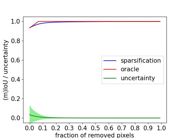
(a) Class car

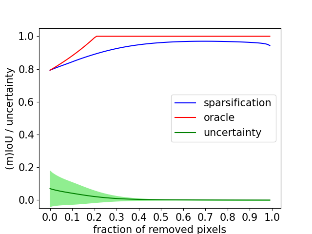
(b) Class terrain

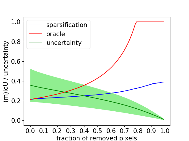
(c) Class bicycle

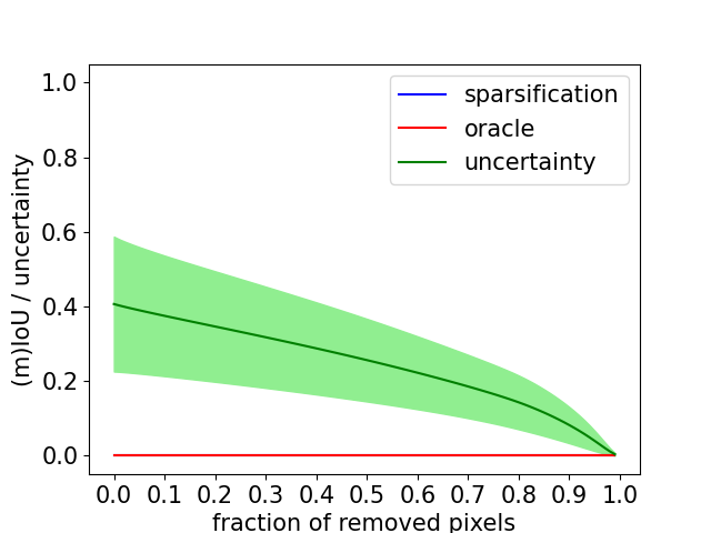
(d) Class bicyclist

Figure 2: Sparsification plots of predictive entropy for several classes with the cross-entropy-trained model. The mean and standard deviation of the uncertainty is given in green.

IV-B Model Training Adaption

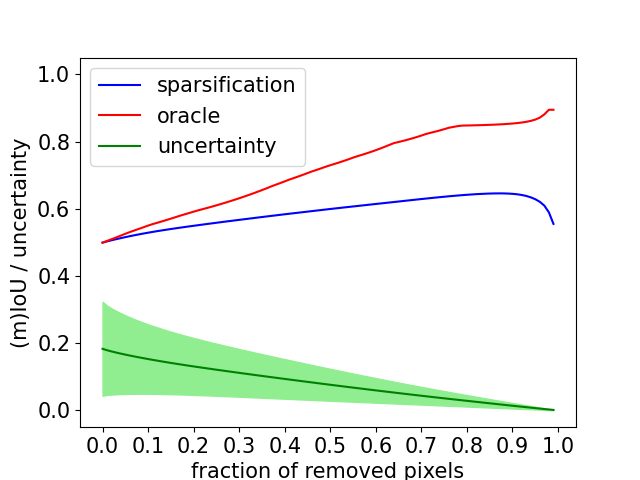
(a) Cross-entropy

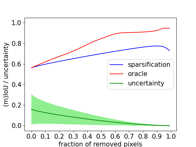
(b) Weighted cross-entropy

Figure 3: Sparsification plots of the predictive entropy over all classes of two models trained with the cross-entropy loss and the weighted cross-entropy loss, respectively. The mean and standard deviation of the uncertainty is given in green.

The above analysis reveals a bad confidence calibration for classes which are generally underrepresented in the data and thus not well learned by the model. To verify this assumption, we conducted the same evaluations on a model which is trained with a weighted loss: the cross-entropy loss is weighted with the respective classes inverse log-frequency within the dataset. We expected a reduced model uncertainty about the underrepresented classes and at the same time a better confidence calibration of them.

When comparing the overall AUSE and sparsification plots (Fig. 3) for the predictive uncertainty, a major improvement of the confidence calibration can be observed. As can be seen in Tab. I, the AUSE for several underrepresented classes improved drastically, though at the expense of other classes which performed well before (e.g. parking, fence).

As Fig. 4 reveals, previously well calibrated classes like car (Fig. 4(a)) still exhibits a reasonable uncertainty estimation. Classes like terrain went through a slight decline of the calibration performance, likely due to the confusion with some underrepresented classes which were given more weight in the calculation of the loss during the training. In the sparsification plot in Fig. 4(b) this is reflected in the curves and can also be seen in the slope of the mean uncertainty of the terrain class points.

For the case of the bicyclist class (Fig. 4(d)), the AUSE increased but solely because the oracle curve is not constantly at an IoU of $0.0$ (compare Tab. I). The previously poor performing classes like bicyclist and even bicycle experienced a major detection improvement (IoU) through the change of the loss function and thus a reduction of the (model) uncertainty, as can be seen in Fig. 4(c). These insights can be used to balance this tradeoff with respect to the desired model performance, e.g. to carefully tune the detection of more safety-critical classes in the context of autonomous driving.

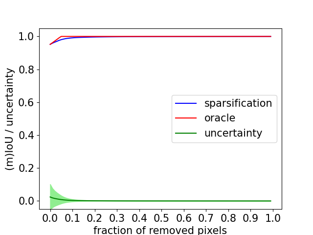
(a) Class car

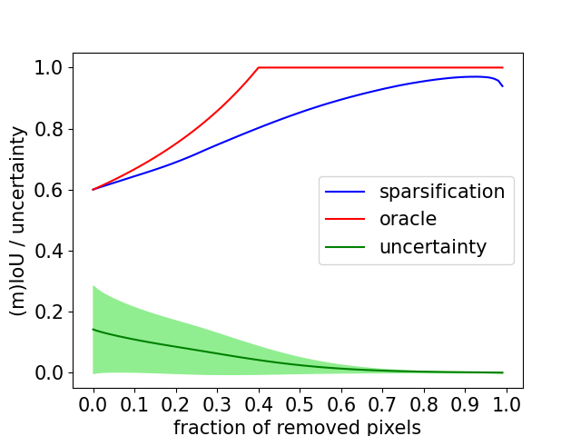
(b) Class terrain

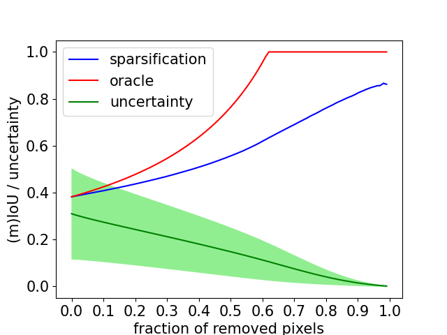
(c) Class bicycle

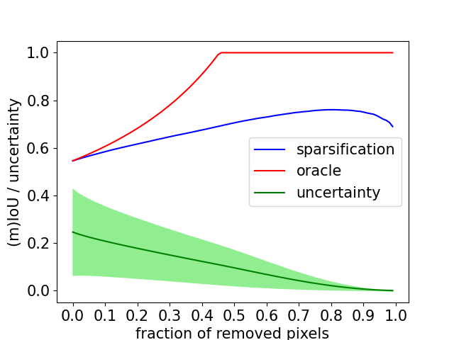
(d) Class bicyclist

Figure 4: Sparsification plots of predictive entropy for several classes with the weighted cross-entropy-trained model. The mean and standard deviation of the uncertainty is given in green.

IV-C Detection and Analysis of Label Problems

For datasets with given labels, a mask can be created which filters only incorrect classifications accompanied by a low uncertainty estimate. This allows us to quickly identify potential label issues which can be further analyzed.

IV-C1 Problems Concerning the Label Hierarchy

The first case can be observed when closely analyzing the detection and calibration performance of the class bicyclist. Despite the detection improvement of the class bicyclist a little drop of the sparsification curve can be observed in Fig. 4(d). This indicates that the model made some wrong predictions (either false positives or false negatives) of the class bicyclist but was at the same time quite confident about its prediction (low uncertainty). Further investigations of all the models’ predictions concerning the class bicyclist reveal that indeed the model had problems with the label hierarchy in this case. Fig. 5 shows a projected LiDAR scan that illustrates this phenomenon. In the left white circle, we find representatives of the classes bicycle and person, in the right one a bicyclist. Nevertheless, since CNNs primarily learn typical local class features, it is understandable when the model predicts a bicycle and a person separately. While in this frame the uncertainty for the two examples are (correctly) high, another example demonstrates the problem resulting from this way of labeling. Fig. 6 shows a rider on a bicycle, labeled as bicyclist (6(a)), which he clearly is but the bicycle is not fully visible. The model predicts a person with a very high confidence, which can be seen Fig. 6(b) and 6(c). These kind of point clusters lead to a drop in the sparsification curve and thus to a worse confidence calibration, despite the rider on the bicycle is also a person without any doubt.

(a) Ground truth labels

(b) Model predictions

(c) Predictive uncertainty

semantic segmentation: road sidewalk parking building vegetation car person fence bicycle trunk bicyclist pole terrain otherground
uncertainty estimation: low high

Figure 5: Example of a confusion of the classes bicycle / person and bicyclist (right circle, compared to left circle). Instead of recognizing the bicyclist as one entity, the model predicts the rider as person and the bicycle as bicyclist, both with high predictive uncertainties.

(a) Ground truth labels

(b) Model predictions

(c) Predictive uncertainty

semantic segmentation: vegetation terrain trunk road bicyclist person pole motorcycle bicycle
uncertainty estimation: low high

Figure 6: Example of a confusion of the classes bicycle / person and bicyclist. Although the person is definitively riding a bicycle, the model predicts the rider as person with a high confidence.

IV-C2 Problems concerning the label

For the second case we found examples of classes which where inconsistently defined. Two examples can be seen in Fig. 7 and Fig. 8. The first one shows a generic sign that is wrongly labeled as traffic sign (Fig. 7(a)), the model assumes it partially belongs to the pole behind it (Fig. 7(b)), in lack of a more suitable class. In the second figure the model detects a fence embedded in a hedge (Fig. 8(b)). This fence is not labeled accordingly, instead it is incorrectly labeled as part of the hedge (Fig. 8(a)). In both cases, the models’ predictive uncertainty is low (Fig. 7(c) and Fig. 8(c)), indicating that there is probably a problem with the provided labels in this region. In these cases, a further inspection helps to identify and mitigate label errors.

(a) Ground truth labels

(b) Model predictions

(c) Predictive uncertainty

(d) Camera image

semantic segmentation: road terrain sidewalk pole trafficsign trunk vegetation building bicyclist motorcycle parking car fence
uncertainty estimation: low high

Figure 7: Example of a wrongly labeled traffic sign. The sign in question is a advertising poster, which can be seen in the camera footage. The model erroneously predicts one side as part of the pole behind it with a low uncertainty.

(a) Ground truth labels

(b) Model predictions

(c) Predictive uncertainty

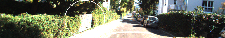
(d) Camera image

semantic segmentation: vegetation trunk sidewalk road car building vegetation fence trafficsign
uncertainty estimation: low high

Figure 8: Example of a gate wrongly labeled as vegetation. The model recognizes a fence with high confidence, which is backed up by the uncertainty image and the camera footage.

V Discussion

Our analyses demonstrated how our proposed metric allows a qualitative and quantitative evaluation of the confidence calibration of a semantic segmentation model. It has several advantages compared to existing confidence calibration metrics for semantic segmentation models:

• Since it is based on the mIoU metric, it does not neglect underrepresented classes and allows an independent confidence calibration evaluation of all classes.

• It does not require any parameter tuning (like accuracy and uncertainty thresholds of the PAvPU metric).

• It does not depend on a specific normalization method of the uncertainty estimates (which is necessary for many uncertainty estimation methods).

From the sparsification plots we know that our model made wrong predictions with low uncertainties. These highly confident but wrong predictions manifest in more or less grave drops in the sparsification curve. Ideally, a well calibrated model would exhibit strictly increasing curves, indicating that the model meets all previously mentioned (compare Sec. II-C) properties:

• accuracy in case of confident predictions

• uncertainty in case of inaccurate predictions

• confidence in case of accurate predictions

There are three possible reasons for highly confident but wrong predictions: 1. the situation is difficult to interpret and the models performance is insufficient, 2. there are problems with the label hierarchy or definition, 3. there are problems with the labels.

In the former situation, the problem does not lie within the labels but rather the model performance. In this case, it is worth analyzing whether the failure case is critical and how to mitigate it. We demonstrated one example measure in Sec. IV-B: adjusting the loss function in favor of underrepresented classes. This can be further adjusted and refined until the model performance meets the requirements. Nevertheless, the other two cases cannot be eliminated by adjusting the model but by questioning the training data (as elaborated in Sec. IV-C).

The second case describes conceptual problems with the labels and their definitions. When there is a problem with the label hierarchy, the model is not able to distinguish between two usually seperated components and the new entity they built when combined. Inconststent labeling in ambiguous situations also falls into this category. Examples for both cases can be observed in Fig. 1. The model detects the rider as a person and the vehicle as a motorcycle, which is not wrong. Despite not riding on a road, the labels define it as one entity, a motorcyclist. Furthermore, the wall on the left side is labeled as fence but the model predicts it as part of the building instead. In both cases it is debatable which definition is closer to the real situation and, above all, which definition is desireable and suitable for downstream tasks.

The third case describes label errors which might be due to weaknesses in the labeling process or human mistakes. Once found they can easily be corrected accordingly.

After identifying problematic classes with the help of the AUSE and sparsification curves, measures can be taken to eliminate the three reasons as far as possible.

In the rare case that the model is not able to learn a representation of a class, the AUSE reaches its limits. As mentioned in Sec. IV-A, the AUSE alone is hard to evaluate. Nevertheless, in this case the respective IoU and the sparsification plots help to detect and alleviate the underlying problem.

VI Conclusion

In this paper we proposed a novel calibration metric for point-wise multi-class classification models. We demonstrated its capabilities in finding limitations in the training process and problems in the label structure. By closely analyzing the results we were able to point out unclear and problematic class definitions and label inconsistencies.

This illustrates how crucial the quality of the database is for the model training and uncertainty estimation, especially when it comes to imbalanced data. When evaluating a models’ calibration, we have to bear in mind the way how the labeling effects the models uncertainty estimation. Thus, we have to be careful with the way, concepts and classes are represented in the labels and the label hierarchy.

Concluding, our analyses yielded important insights about uncertainty estimation in semantic segmentation models, their calibration and the role the data representation plays.

To further advance in this field of research, it is important to entangle the different types of uncertainty and gain a deeper understanding of their role in model training. This might provide access to identifying and alleviating limiting factors within the process, such as data underrepresentation or inconsistent class definitions and might even have an impact on related tasks like domain adaptation or outlier detection.

References

- [1] F. P. J. Piewak, “LiDAR-based Semantic Labeling (Automotive 3D Scene Understanding),” Ph.D. dissertation, Karlsruher Institut für Technologie, 2020.
- [2] Y. He, H. Yu, X. Liu, Z. Yang, W. Sun, Y. Wang, Q. Fu, Y. Zou, and A. Mian, “Deep Learning based 3D Segmentation: A Survey,” arXiv, 2021.
- [3] J. Behley, M. Garbade, A. Milioto, J. Quenzel, S. Behnke, J. Gall, and C. Stachniss, “Towards 3D LiDAR-based Semantic Scene Understanding of 3D Point Cloud Sequences-The SemanticKITTI,” in Int. J. Robot. Res., 2021.
- [4] C. Guo, G. Pleiss, Y. Sun, and K. Q. Weinberger, “On Calibration of Modern Neural Networks,” in ICML, 2017.
- [5] Y. Gal, “Uncertainty in Deep Learning,” Ph.D. dissertation, University of Cambridge, 2016.
- [6] B. Lakshminarayanan, A. Pritzel, and C. Blundell, “Simple and Scalable Predictive Uncertainty Estimation using Deep Ensembles,” in NIPS, 2017.
- [7] A. Kendall and Y. Gal, “What Uncertainties do we Need in Bayesian Deep Learning for Computer Vision?” in NIPS, 2017.
- [8] F. Arnez, H. Espinoza, A. Radermacher, and F. Terrier, “A Comparison of Uncertainty Estimation Approaches in Deep Learning Components for Autonomous Vehicle Applications,” in IJCAI - Workshop, 2020.
- [9] J. Mukhoti, A. Kirsch, J. V. Amersfoort, P. H. S. Torr, and Y. Gal, “Deterministic Neural Networks with Appropriate Inductive Biases Capture Epistemic and Aleatoric Uncertainty,” arXiv, 2021.
- [10] J. Huang and S. You, “Point Cloud Labeling using 3D Convolutional Neural Network,” in ICPR, 2016.
- [11] H.-Y. Meng, L. Gao, Y. Lai, and D. Manocha, “VV-Net: Voxel VAE Net with Group Convolutions for Point Cloud Segmentation,” in ICCV, 2018.
- [12] C. R. Qi, L. Yi, H. Su, and L. J. Guibas, “PointNet++: Deep Hierarchical Feature Learning on Point Sets in a Metric Space,” in NIPS, 2017.
- [13] Y. Li, R. Bu, M. Sun, W. Wu, X. Di, and B. Chen, “PointCNN: Convolution On X-Transformed Points,” in NIPS, 2018.
- [14] J. Yang, Q. Zhang, B. Ni, L. Li, J. Liu, M. Zhou, and Q. Tian, “Modeling Point Clouds with Self-Attention and Gumbel Subset Sampling,” in CVPR, 2019.
- [15] A. Milioto, I. Vizzo, J. Behley, and C. Stachniss, “RangeNet++: Fast and Accurate LiDAR Semantic Segmentation,” in IROS, 2019.
- [16] E. E. Aksoy, S. Baci, and S. Cavdar, “SalsaNet: Fast Road and Vehicle Segmentation in LiDAR Point Clouds for Autonomous Driving,” in IV, 2019.
- [17] B. Wu, A. Wan, X. Yue, and K. Keutzer, “SqueezeSeg: Convolutional Neural Nets with Recurrent CRF for Real-Time Road-Object Segmentation from 3D LiDAR Point Cloud,” in ICRA, 2017.
- [18] C. Xu, B. Wu, Z. Wang, W. Zhan, P. Vajda, K. Keutzer, and M. Tomizuka, “SqueezeSegV3: Spatially-Adaptive Convolution for Efficient Point-Cloud Segmentation,” in ECCV, 2020.
- [19] A. Paszke, A. Chaurasia, S. Kim, and E. Culurciello, “ENet: A Deep Neural Network Architecture for Real-Time Semantic Segmentation,” arXiv, 2016.
- [20] J. Xu, R. Zhang, J. Dou, Y. Zhu, J. Sun, and S. Pu, “RPVNet: A Deep and Efficient Range-Point-Voxel Fusion Network for LiDAR Point Cloud Segmentation,” arXiv, 2021.
- [21] R. Cheng, R. Razani, E. Taghavi, E. Li, and B. Liu, “(AF)2-S3Net: Attentive Feature Fusion with Adaptive Feature Selection for Sparse Semantic Segmentation Network,” in CVPR, 2021.
- [22] E. Hüllermeier and W. Waegeman, “Aleatoric and epistemic uncertainty in machine learning: an introduction to concepts and methods,” Machine Learning, 2021.
- [23] Y. Gal and Z. Ghahramani, “Dropout as a Bayesian Approximation: Representing Model Uncertainty in Deep Learning,” in ICML, 2015.
- [24] Y. Gal, J. Hron, and A. Kendall, “Concrete Dropout,” in NIPS, 2017.
- [25] A. Kamath, D. Gnaneshwar, and M. Valdenegro-Toro, “Know Where To Drop Your Weights: Towards Faster Uncertainty Estimation,” arXiv, 2020.
- [26] J. Z. Liu, J. Paisley, M.-A. Kioumourtzoglou, and B. A. Coull, “Accurate Uncertainty Estimation and Decomposition in Ensemble Learning,” arXiv, 2019.
- [27] S. Cygert, B. Wróblewski, K. Woźniak, R. Słowiński, and A. Czyżewski, “Closer Look at the Uncertainty Estimation in Semantic Segmentation under Distributional Shift,” in IJCNN, 2021.
- [28] J. Nixon, M. Dusenberry, G. Jerfel, T. Nguyen, J. Liu, L. Zhang, and D. Tran, “Measuring Calibration in Deep Learning,” arXiv, 2019.
- [29] J. Mukhoti and Y. Gal, “Evaluating Bayesian Deep Learning Methods for Semantic Segmentation,” arXiv, 2021.
- [30] E. Ilg, Özgün Çiçek, S. Galesso, A. Klein, O. Makansi, F. Hutter, and T. Brox, “Uncertainty Estimates and Multi-Hypotheses Networks for Optical Flow,” in ECCV, 2018.
- [31] F. K. Gustafsson, M. Danelljan, and T. B. Schon, “Evaluating scalable bayesian deep learning methods for robust computer vision,” in CVPR, June 2020.
- [32] J. Behley, M. Garbade, A. Milioto, J. Quenzel, S. Behnke, C. Stachniss, and J. Gall, “SemanticKITTI: A Dataset for Semantic Scene Understanding of LiDAR Sequences,” in CVPR, 2019.
- [33] L. T. Triess, D. Peter, C. B. Rist, and J. M. Zöllner, “Scan-based Semantic Segmentation of LiDAR Point Clouds: An Experimental Study,” in IV, 2020.
- [34] T. Cortinhal, G. Tzelepis, and E. E. Aksoy, “SalsaNext: Fast, Uncertainty-aware Semantic Segmentation of LiDAR Point Clouds for Autonomous Driving,” arXiv, 2020.
- [35] F. Piewak, P. Pinggera, M. Schäfer, D. Peter, B. Schwarz, N. Schneider, M. Enzweiler, D. Pfeiffer, and M. Zöllner, “Boosting LiDAR-based semantic Labeling by Cross-Modal Training Data Deneration,” in ECCV, 2019.
- [36] L. Triess. (2019) Scripts for SemanticKITTI Dataset Statistics. [Online]. Available: https://github.com/ltriess/semantic˙kitti˙stats