The Signum-Gordon shock waves in 2+1 and 3+1 dimensions

Abstract

We investigate shock wave solutions in the Signum-Gordon model with field discontinuity at the light cone. The exact solutions to this problem in the dimensions 2+1 and 3+1 are given. We show that the volume of the disk/ball with radius $t$ multiplied by the value of the field discontinuity on the surface of the light cone equals the energy of the solution inside the light cone at time $t$. In contrast to shock waves in one spatial dimension, the non-homogeneous signum-Gordon equation with the Dirac’s delta force supports solutions in higher dimensions. We examine the degradation of the shock wave after turning off the delta-force.

I Introduction

The signum-Gordon (SG) model is perhaps the most straightforward scalar field model with non-analytic potential. The model gets its name from the fact that the sign function, $\frac{dV}{d\phi}=\lambda\;{\rm sgn}(\phi)$, determines the force term in the equation of motion Arodz et al. (2007). In contrast to the Klein-Gordon (KG) model, which has a quadratic potential $\frac{dV}{d\phi}=m^{2}\phi$, the force in the SG model does not disappear for arbitrarily small deviation from the minimum $\phi=0$. Because of this, the force is known as a threshold force. The SG potential is piecewise linear, with the potential $V(\phi)=\lambda\;|\phi|$. Despite its apparent simplicity, the model has extremely complex dynamics, Hahne et al. (2020a).

Potentials in conventional field theoretic models have quadratic minima. The dynamics of the KG field can be used to estimate how these fields behave at minima in various physical applications. The solutions of the KG equations (within an approximation domain) can approximate the solutions of various physical models. A similar relationship exists between models with non-analytic potentials at their minima and the SG model. In other words, the dynamics of small-amplitude oscillations is a general phenomenon that may be observed in other models of the same class, also known as models with V-shaped potentials, Arodz et al. (2005). The first example of this type of model was given in Arodz (2002), which addressed a modified mechanical system of inverted pendulums and their field theoretic limit. Mechanical models of this type with only a few degrees of freedom were previously well-known in the literature as models that support chaotic behavior that emerges in grazing biffurcation; for instances, see Thompson and Ghaffari (1983); Nusse et al. (1994); Chin et al. (1994). They are also discussed in Rodriguez-Coppola’s 1992 paper on dynamics of the electron gas in two dimensions Rodriguez-Coppola and Perez-Alvarez (1992) and in the article on plasma physics Ishiguro et al. (1997). It was recently proved in Adam et al. (2018) that the Skyrme model decomposes into two coupled BPS submodels, one of which has a V-shaped potential. This is a crucial example because it demonstrates how a model with a V-shaped potential may emerge from a model with no potential.

The SG model has a few common characteristics. One of these is the scaling symmetry, which permits the existence of self-similar solutions Arodz et al. (2007). Another very characteristic mark of such models is the presence of compactons, i.e. solutions with strictly compact support. The presence of compactons, or solutions with strictly compact support, is another defining trait of these models. Topological compactons, such as the compact kink Arodz (2002), as well as non topological compactons, such as the precise compact oscillon Arodz et al. (2008); Arodz and Swierczynski (2011); Świerczyński (2021) or compact Q-balls Arodz and Lis (2008, 2009); Klimas and Livramento (2017); Klimas et al. (2019), are both possible. Finally, a quadratic potential cannot be used to mimic the V-shaped potential near its minimum. This indicates that oscillations with modest amplitudes are inherently nonlinear. In other words, for models with V-shaped potentials, the harmonic oscillator paradigm does not apply.

In this study, we look into the shock waves family of SG model solutions. To obtain this unique family of solutions, the model’s partial differential equations are reduced to an ordinary equation. The SG model in 1+1 dimensions is the model being discussed, and exact solutions of this kind were originally provided in Arodz et al. (2005). The waves have two fronts that move in opposite directions at the speed of light. The field is nontrivial within the light cone and zero outside of it. The field is not continuous at the surface of the light cone. The SG model in 1+1 dimensions with quadratic perturbation provides exact shock wave solutions as well Klimas (2007). We recently explored these solutions numerically and analytically, and we discovered that non-exact configurations break down into a series of compact oscillons Hahne et al. (2020b). Shock wave-like structures of this type can be generated during the scattering process of compact oscillons, as demonstrated in Hahne et al. (2020a). This scattering is a mechanism that transfers the energy of some SG configurations into smaller structures that produce a radiation field.

In this paper, we extend the concept of shock waves in the SG model to include two and three spatial dimensions. Using analytical and numerical techniques, we investigate solutions with discontinuities at the light cone. The paper is organized as follows: is Section (II) we develop a generic analytic solution to the shock wave field and its total energy. We also address the delta force at the light cone, which is a nonhomogeneous term in the SG equation. Section (III) focuses on the numerical solution of a full-time dependent problem. Then, in Section (IV), we give our comments and remarks.

II Exact shock waves

II.1 The shock wave equation in $n+1$ dimensions

In $n+1$ dimensions, the SG equation takes the form of a Klein-Gordon equation with the mass term substituted by the ${\rm sgn}(\phi)$ function, i.e.

$$(\partial^{2}_{t}-\nabla^{2})\phi(t,\vec{x})+{\rm sgn}\phi(t,\vec{x})=0.$$ (II.1)

The vacuum configuration $\phi=0$ is an explicit solution of equation (II.1) if ${\rm sgn}(0):=0$. In this study, we will use this definition of the signum function. Using spherical coordinates, one obtains (II.1) of the type

$$\left(\partial^{2}_{t}-\partial^{2}_{r}-\frac{n-1}{r}\partial_{r}-\frac{1}{r^{2}}\nabla^{2}_{S^{n-1}}\right)\phi(t,\vec{x})+{\rm sgn}(\phi(t,\vec{x}))=0,$$ (II.2)

where $r=\sqrt{x_{1}^{2}+\ldots+x_{n}^{2}}$ is the radial coordinate and the operator $\nabla^{2}_{S^{n-1}}$ is determined by the set of angular variables. We are looking for solutions with spherical symmetry, which means they do not depend on the angles. As a result, $\nabla^{2}_{S^{n-1}}\phi(t,r)=0$, and the field equation has the following form

$$\left(\partial^{2}_{t}-\partial^{2}_{r}-\frac{n-1}{r}\partial_{r}\right)\phi(t,r)+{\rm sgn}(\phi(t,r))=0.$$ (II.3)

New variables can be chosen as $x_{\pm}:=\frac{1}{2}(r\pm t)$. These are the coordinates of the light cone. As a result, the scalar field $\phi=\phi(x_{+},x_{-})$ satisfies the equation

$$-\partial_{+}\partial_{-}\phi-\frac{n-1}{2}\frac{\partial_{+}\phi+\partial_{-}\phi}{x_{+}+x_{-}}+{\rm sgn}(\phi)=0.$$ (II.4)

This equation has a subset of solutions that obey an ordinary differential equation. Such solutions depend on a single variable that is a product of light cone coordinates $z:=x_{+}x_{-}$, and so take the form

$$\phi(x_{+},x_{-})=W(z)\qquad{\rm where}\qquad z=\frac{1}{4}(r^{2}-t^{2}).$$ (II.5)

The partial equation (II.4) is simplified to the following one

$$-zW^{\prime\prime}-\frac{n+1}{2}W^{\prime}+{\rm sgn}(W)=0$$ (II.6)

under the assumption regarding the class of solutions. We shall assume that the function $W(z)$ is nontrivial inside the light cone $z<0$ and equal to zero outside the light cone $z>0$. Since ${\rm sgn}(0):=0$ the constant solution $W(z)=0$ solves the equation for the region $z>0$.

We will investigate functions with it discontinuities at the light cone $r=t$ because we are interested in shock waves. In Arodz et al. (2006), such shock wave solutions in one spatial dimension were investigated. Following this paper, we will look at expressions

$$\phi(z)=\theta(-z)W(z)$$ (II.7)

where $\theta(-z)$ is the Heaviside step function. The left hand side of the SG equation (II.4) (in variable $z$) will be denoted by

$$F(\phi):=-\big{(}z\phi^{\prime}(z)\big{)}^{\prime}-\frac{n-1}{2}\phi^{\prime}(z)+{\rm sgn}(\phi(z))$$ (II.8)

According to Vladimirov (1971), the result of a distribution $f(z)$ (generalized function) on a test function $\varphi(z)$ is represented by $(f,\varphi)\equiv\int_{-\infty}^{\infty}dzf(z)\varphi(z)$. The Dirac’s delta distribution, in particular, acts on a test function according to $(\delta,\varphi)=\int_{-\infty}^{\infty}dz\;\delta(z)\varphi(z)=\varphi(0)$. When (II.7) is plugged into (II.8), the expression

$$(F(\phi),\varphi(z))=\frac{n-1}{2}W(0)\varphi(0)+\int_{-\infty}^{\infty}dz\theta(-z)\left[-(zW^{\prime}(z))^{\prime}-\frac{n-1}{2}W^{\prime}(z)+{\rm sgn}(W(z))\right]\varphi(z)$$

is obtained. Given that $W(z)$ is an (II.6) solution, this expression yields a term proportional to Dirac’s delta

$$(F(\phi),\varphi(z))=\left(C_{n}\,\delta(z),\varphi(z)\right),\qquad C_{n}\equiv\frac{n-1}{2}W(0).$$ (II.9)

It should be noted that this results can also be obtained by using the effective formulas

$$\theta^{\prime}(-z)=-\delta(z),\quad z\delta(z)=0,\quad z\delta^{\prime}(z)=-\delta(z),\quad{\rm sgn}(\theta(-z)W(z))=\theta(-z){\rm sgn}(W(z)).$$

We conclude that the expression (II.7) is a solution of the homogeneous equation $F(\phi)=0$ for $n=1$, ($C_{1}=0$). The solution is derived by solving an ordinary equation (II.6) with the radial coordinate $r\geq 0$ replaced by $x\in{\mathbb{R}}$. For $n\neq 1$, on the other hand, the term $F(\phi)$ does not disappear ($C_{n}\neq 0$), and so the expression (II.7) is proportional to the fundamental solution $D(z)$ of the distributional equation

$$\Big{(}F(D(z)),\varphi(z)\Big{)}=(\delta(z),\varphi(z))$$ (II.10)

where $\phi(z)=D(z)$ holds true for $W(0):=\frac{2}{n-1}$.

There are solutions of the SG equation (or perturbed equations of this kind, Klimas (2007)) in $n=1$ spatial dimension in the form of shock waves, i.e. solutions with fixed value of discontinuity on the surface of the light cone, as illustrated in Arodz et al. (2005). Similar-in-form solutions can occur in higher dimensions $n\geq 2$ if an extra force exists on the surface of the light cone. They are, in other words, solutions to a non-homogeneous SG equation (II.9) with a delta term proportional to the value of a discontinuity $W(0)$.

Furthermore, if we do not fix $W(0)$, we can find a one parameter family of solutions that represent a generalization of shock waves in 1+1 dimensions. It is believed that such solutions exist in higher dimensions $n\geq 2$. Of course, one can look at numerical solutions to the problem, but it is much more intriguing to look at analytical solutions first. We will discuss briefly on these new solutions below. More information is provided in (II.3) and (II.4).

The shock wave is made up of analytical solutions with domains on small segments. When such solutions (patches) are matched on $z<0$, they produce the function $W(z)$. They are known as partial solutions. To derive exact formulas for partial solutions, we assume $W(z)$ to be a non-constant expression, that is, it can be equal to zero only in specific isolated places along the $z$ axis. With the exception of these places where $W(z)$ vanishes, we have either $W>0$ or $W<0$. In this situation, it is easier to rewrite the expression ${\rm sgn}(W)=\pm 1$ as ${\rm sgn}(W_{k})=(-1)k$, where $k=0,1,\ldots$ labels consecutive partial solutions $W_{k}$. (II.6) is equivalent to a collection of non-homogeneous linear equations

$$-zW_{k}^{\prime\prime}-\frac{n+1}{2}W_{k}^{\prime}+(-1)^{k}=0.$$ (II.11)

There are two groups of solutions to the equation (II.11), namely

$$W_{k}(z)=\alpha_{k}+\beta_{k}\ln(-z)+(-1)^{k}z\qquad{\rm for}\qquad n=1$$ (II.12)

and

$$W_{k}(z)=\alpha_{k}+\beta_{k}(-z)^{-\frac{n-1}{2}}+\frac{2(-1)^{k}}{n+1}z,\qquad{\rm for}\qquad n\geq 2.$$ (II.13)

The first kind, (II.12), has been widely explored Hahne et al. (2020b); Arodz et al. (2006), whereas the second type, (II.13), is the focus of this paper.

The free constant $\alpha_{0}=W_{0}(0)$ parametrizes the solutions. Using $\beta_{0}=0$, one obtains a partial solution $W_{0}$ on the segment $-a_{0}<z<0$, where $a_{0}>0$. For $n=1$, one obtains $\alpha_{0}=a_{0}$, and for $n\geq 2$, one gets $\alpha_{0}=\frac{n+1}{2}a_{0}$. The solution $W_{1}(z)$ corresponds to $W_{0}(-a_{0})$, i.e. it satisfies $W_{1}(-a_{0})=0$ as well as $W^{\prime}_{1}(-a_{0})=W^{\prime}_{0}(-a_{0})$. These conditions allow us to calculate $\alpha_{1}$, $\beta_{1}$, and the next zero $z=-a_{1}$, $W_{1}(-a_{1})=0$. This procedure can be repeated indefinitely. The answer is found by formulating and solving several recurrence relations. Sections (II.3) and (II.4) discuss a concrete form of partial solutions; see Figures 1 and 2. Now we shall look at some general shock wave energy properties.

II.2 The shock wave’s energy

II.2.1 The distribution of energy within a shock wave

The zone where the scalar field is excited expands with time as the shock wave spreads. The wave’s energy is contained within the light cone $r<t$. The form of the integral representing energy is

$$E(t)=\int_{K(0,t)}d^{n}x\left[\frac{1}{2}(\partial_{t}\phi)^{2}+\frac{1}{2}(\partial_{i}\phi)^{2}+|\phi|\right]$$ (II.14)

where the solution’s support $K(0,t)$ is a $n-$sphere with a center at $\vec{r}=0$ and a radius $r$. It should be noted that this integral excludes the wave’s discontinuity, which is located at the light cone $r=t$. In summary, we compute wave energy by dividing it into three distinct zones related by the light cone:

1. $r<t$: inner field, where energy behaves well. This is covered in Section (II.2.2);

2. $r=t$: on the cone surface, where the energy is undefined due to the field discontinuity and the leading delta term (see equation II.10). This is addressed in Section (II.2.3);

3. $r>t$: outside the cone, trivial vacuum.

The idealized exact solution has infinite gradient energy associated with the field discontinuity at the light cone. It results in a significant and sensitive discrepancy between the numerical simulation and the analytical solutions corresponding to an idealized situation. Even still, physical applications exist for exact solutions with unlimited energy (such as shock waves and self-similar solutions). Field configurations that are very close to such solutions (often over finite time intervals) are observed in certain physical processes, such as the scattering of compact oscillons Hahne et al. (2020a). In Hahne et al. (2020b), we compare the radiation field obtained during a scattering process to shock-like waves obtained for some specific starting data. The similarity between the two configurations is extremely striking.

II.2.2 Energy inside the light-cone

Because $\phi$ is just a function of $t$ and $r$, the expression (II.14) reduces to

$$E(t)=\int_{\mathcal{S}_{n}}d\Omega\int_{0}^{t}dr\,r^{n-1}\sum_{k=0}^{k_{\rm max}(t)}H_{k}(t,r)$$ (II.15)

where $W_{k}(z)$ solutions are supplied by (II.12) and (II.13), and $W^{\prime}_{k}(z):=\frac{dW_{k}(z)}{dz}$. The contributions to energy density from partial solutions are of the form

$$H_{k}(t,r)=\dfrac{r^{2}+t^{2}}{8}W_{k}^{\prime 2}(z)+(-1)^{k}W_{k}(z),\qquad z=\frac{1}{4}(r^{2}-t^{2}).$$

In (II.15), $k_{\rm max(t)}$ represents the greatest index of partial solution $W_{k}(z)$ that fits inside the light cone at given $t$. The number of partial solutions that constitute the shock wave at time $t$ is finite and grows with time. The area of a unit sphere in $n$ spatial dimensions is represented by the integral $\int_{\mathcal{S}_{n}}d\Omega$.

The expressions $W_{k}(z)$ and $W^{\prime}_{k}(z)$ are non zero on the open segment $-a_{k}<z<-a_{k-1}$ but equal zero outside this segment. As a result, $W(-a_{k})=0$. The algebraic representation of zeros $a_{k}$ varies with the number of spatial dimensions. We will denote $i\equiv k_{\rm max}(t)$ to simplify the notation. The $i-$th zero appears at $r=0$ at the instant $t_{i}=2\sqrt{a_{i}}$. The wave has $i+1$ partial solutions identified by $k=0,1,\ldots,i$ in the interval $t_{i-1}<t<t_{i}$. The energy (II.15) can be written in a way that makes explicit the contribution of each partial solution

$$E(t)=\sum_{k=0}^{i}E_{k}(t).$$ (II.16)

Expressions $E_{k}(t)$, $k=0,1,\ldots,i-1$ are energies of first $i$ partial solutions localized inside shells with radii $c_{k}(t)\leq r\leq c_{k-1}(t)$ and $E_{i}(t)$ represents the energy of a central partial solution inside the ball $0\leq r\leq c_{i-1}(t)$, where scalar field radial running zeros $\phi(t,r)$ have the form

$$c_{k}(t):=\sqrt{t^{2}-4a_{k}}.$$ (II.17)

The crucial thing to remember about (II.16) is that the sum has numerous cancelations before reducing to a simple formula.

$$E(t)=\int_{\mathcal{S}_{n}}d\Omega\int drr^{n-1}[\phi]_{z=0}={\rm vol}_{n}(t)[\phi]_{z=0}$$

with ${\rm vol_{n}(t)}$ denoting the volume of a $n$-dimensional ball of radius $t$ and $[\phi]_{z}=0$ denoting the field discontinuity at the light cone. Sections (II.3) for $n=2$ and (II.4) for $n=3$ demonstrate this reduction. It is worth noting that shock waves in one spatial dimension have energy that may be expressed in a similar way, with ${\rm vol_{1}}(t)=2t$ and $[\phi]_{z}=0=a_{0}$. It means that the energy of a wave inside the light cone increases as time passes

$$E(t)={\rm vol}_{n}(t)\;[\phi]_{z=0},\qquad{\rm for}\qquad n=1,2,3.$$ (II.18)

II.2.3 Energy on the light cone’s surface

The energy estimated thus far is contained within the wave’s light-cone and does not account for its surface. This is dealt with in this section. In The one-dimensional shock wave has been thoroughly studied in Hahne et al. (2020b), the one-dimensional shock wave has been thoroughly explored. The field discontinuities at the cone surface provide a problem, resulting in an infinite gradient in the $phi$ profile. For $n=1$, we have $\partial_{x}\phi(t,x)|_{x\sim{}\pm t}\simeq\delta(x\mp t)$, which is squared inside the energy functional and hence meaningless as a distribution. Still, this leads to an intriguing field dynamic: the undefined spike serves as a reservoir from which the inner-cone field pulls energy, expanding as in the expression (II.18). Of course, the energy of the discretized (numerical) system must not only be clearly characterized, but it must also be conserved. From an analytic and numerical standpoint, regularization of the delta is sufficient to ensure both Hahne et al. (2020b).

Although regularization is a method of having a well-defined energy density, it adds an extra parameter $\varepsilon$ to the energy, which has certain consequences. First, the regularization ’$\varepsilon$’ appears in the final computed energy as a denominator, indicating that it does not converge for $\varepsilon\rightarrow 0$. Second, it smoothes out the field discontinuity (turning it into a slope), affecting the gradient term of the energy density. It is what defines and limits it. Third, because the field is no longer discontinuous, the cone surface is now localized in a narrow region $(t-\varepsilon)<x<(t+\varepsilon)$ rather than at $x=t$. As a result, its surface acquires one dimension: it is no longer $(n-1)$-dimensional (the number of spatial dimensions of the system being $n$), but $n$-dimensional. We show that a lower value of $\varepsilon$ results in a steeper slope of field values and a higher density of energy, whereas a higher value results in a gentler slope and a lower density of energy. Fourth, it implies that the reservoir is finite (although orders of magnitude larger in energy density than the remaining field depending on the value of $\varepsilon$). Because wave expansion consumes energy, it can only continue as long as the reservoir is not drained. As a result, the inner-field only has so much energy to increase, implying that it will only be a shock-wave for so long.

We studied the anatomy of the discontinuity and how energy from the reservoir is transferred to the wave at initial moments of evolution (up to about $t=a/\varepsilon$) in $n=1$ spacial dimensions using numerical simulations and analytic solutions to regularized initial conditions (quasi-shock-waves) Hahne et al. (2020b).

II.3 Shock waves in $2+1$ dimensions

II.3.1 Partial solutions and recurrence relations

The formula

$$W_{k}(z)=\alpha_{k}+\frac{\beta_{k}}{\sqrt{-z}}+\frac{2}{3}(-1)^{k}z,\qquad{\rm where}\qquad z<0$$ (II.19)

gives the partial solutions in $n=2$ spatial dimensions. The parameter $\beta_{0}=0$ is used to avoid the field’s singularity at the light cone $z=0$. The first zero $z=-a_{0}$ is such that $W_{0}(-a_{0})=0$, implying that $\alpha_{0}=\frac{2}{3}a_{0}$. It gives

$$W_{0}(z)=\frac{2}{3}(z+a_{0}).$$ (II.20)

This parameter determines the field discontinuity at the light cone

$$[\phi]_{z=0}:=\lim_{z\rightarrow 0-}\phi(z)-\lim_{z\rightarrow 0+}\phi(z)=\lim_{z\rightarrow 0-}W_{0}(z)=\frac{2}{3}a_{0}.$$ (II.21)

Alternatively, the discontinuity can be specified as an independent parameter that determines the value of $a_{0}$. Recurrence relations can be used to determine all of the other parameters and zeros. The initial zero $z=-a_{0}$ is also a $W_{1}(z)$ zero. In terms of $a_{0}$, $\alpha_{1}$ can be eliminated. Similarly, using the constraint $W_{k}(-a_{k}-1)=0$ parameters $\alpha_{k}$ can be eliminated. It provides

$$W_{k}(z)=(-1)^{k}\left[\frac{2}{3}(z+a_{k-1})+b_{k}\left(\frac{1}{\sqrt{-z}}-\frac{1}{\sqrt{a_{k-1}}}\right)\right],\qquad k=1,2,\ldots$$ (II.22)

where $b_{k}\equiv(-1)^{k}\beta_{k}$. The first derivative of the solution $W(z)$ is continuous $W^{\prime}(z):=\frac{dW}{dz}$ at the corresponding points, i.e. $W^{\prime}_{k}(-a_{k}-1)=W^{\prime}_{k}-1(-a_{k}-1)$. It leads to the recurrence relations

$$b_{k}=-b_{k-1}-\frac{8}{3}a_{k-1}^{3/2}\qquad{\rm where}\qquad b_{0}=0.$$ (II.23)

As a result, coefficients $b_{k}$ are given in terms of a sum of all parameters $a_{n}$ with $n<k$.

$$b_{k}=\frac{8}{3}\sum_{n=0}^{k-1}(-1)^{n+k}a_{n}^{3/2},\qquad k=1,2,\ldots.$$ (II.24)

The $k-$th zero $z=-a_{k}$ is achieved by solving the equation $W_{k}(-a_{k})=0$, which may be expressed as a second order equation for $\sqrt{a_{k}}$

$$(\sqrt{a_{k}})^{2}+\sqrt{a_{k-1}}\sqrt{a_{k}}+\frac{3}{2}\frac{b_{k}}{\sqrt{a_{k-1}}}=0,\qquad k=1,2,\ldots$$ (II.25)

When one solves this equation with regard to $\sqrt{a_{k}}$ and takes the square of the result, one obtains

$$a_{k}=s_{k}a_{k-1}=\left(\prod_{i=0}^{k}s_{i}\right)a_{0},\qquad k=1,2,\ldots$$ (II.26)

where

$$s_{0}\equiv 1,$$ (II.27)

$$s_{k}\equiv\frac{1}{2}\Big{(}1-\xi_{k}-\sqrt{1-2\xi_{k}}\Big{)},\qquad k=1,2,\ldots.$$ (II.28)

The expression $\xi_{k}$ is as follows:

$$\xi_{k}\equiv 8\sum_{n=0}^{k-1}(-1)^{n+k}\left(\frac{a_{n}}{a_{k-1}}\right)^{3/2}=8\sum_{n=0}^{k-1}(-1)^{n+k}\left(\frac{\prod_{i=0}^{n}s_{i}}{\prod_{j=0}^{k-1}s_{j}}\right)^{\frac{3}{2}}.$$ (II.29)

It is worth noting that each zero $a_{k}$ is proportionate to $a_{0}$. We can cast partial solutions $W_{k}(z)$ in the form

$$W_{0}(z) =\frac{2}{3}(z+a_{0}),$$ (II.30)

$$W_{k}(z) =\frac{2}{3}(-1)^{k}\frac{\sqrt{d_{k}}+\sqrt{-z}}{\sqrt{-z}}\Big{(}\sqrt{a_{k}}-\sqrt{-z}\Big{)}\Big{(}\sqrt{-z}-\sqrt{a_{k-1}}\Big{)},\qquad k=1,2,\ldots$$ (II.31)

where their zeros are clear by defining expression

$$d_{k}\equiv\frac{1}{2}\Big{(}1-\xi_{k}+\sqrt{1-2\xi_{k}}\Big{)}a_{k-1},\qquad k=1,2,\ldots$$

where $\sqrt{a_{k-1}}<\sqrt{-z}<\sqrt{a_{k}}$. The expressions (II.26)-(II.29) are recurrence relations that determine the zeros of the function $W(z)$. In contrast to shock waves in one spatial dimension, the zeros of waves in two dimensions are supplied by analytical expressions. We plot the function $W(z)$ as well as the shock wave in $n=2$ spatial dimensions in Fig.1.

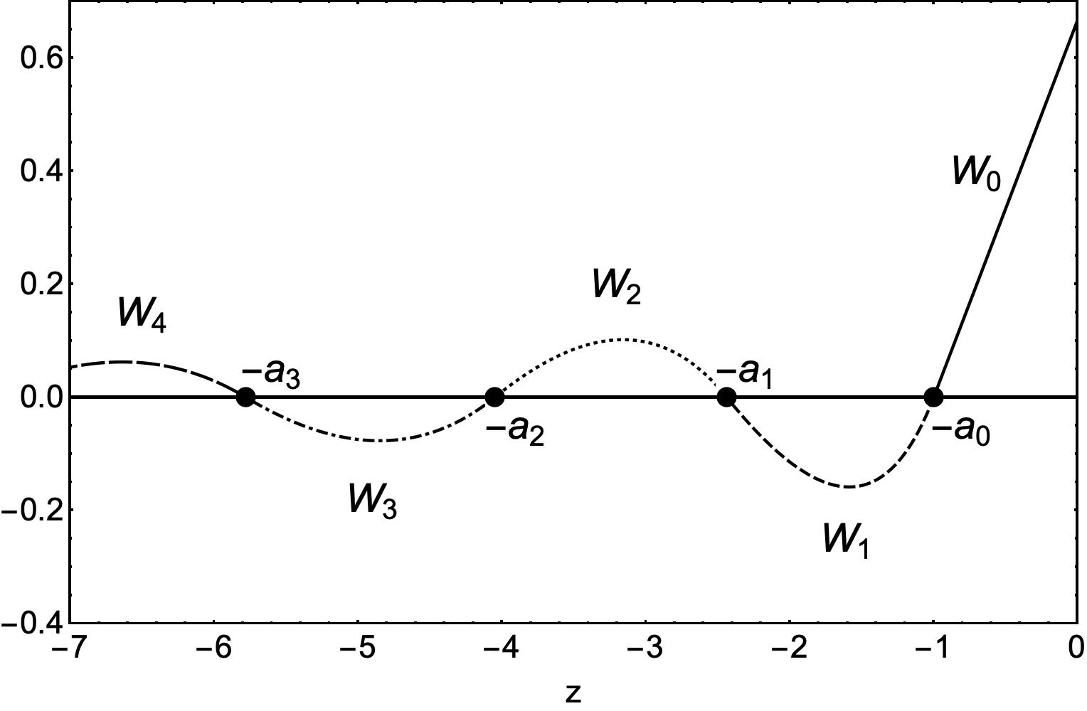
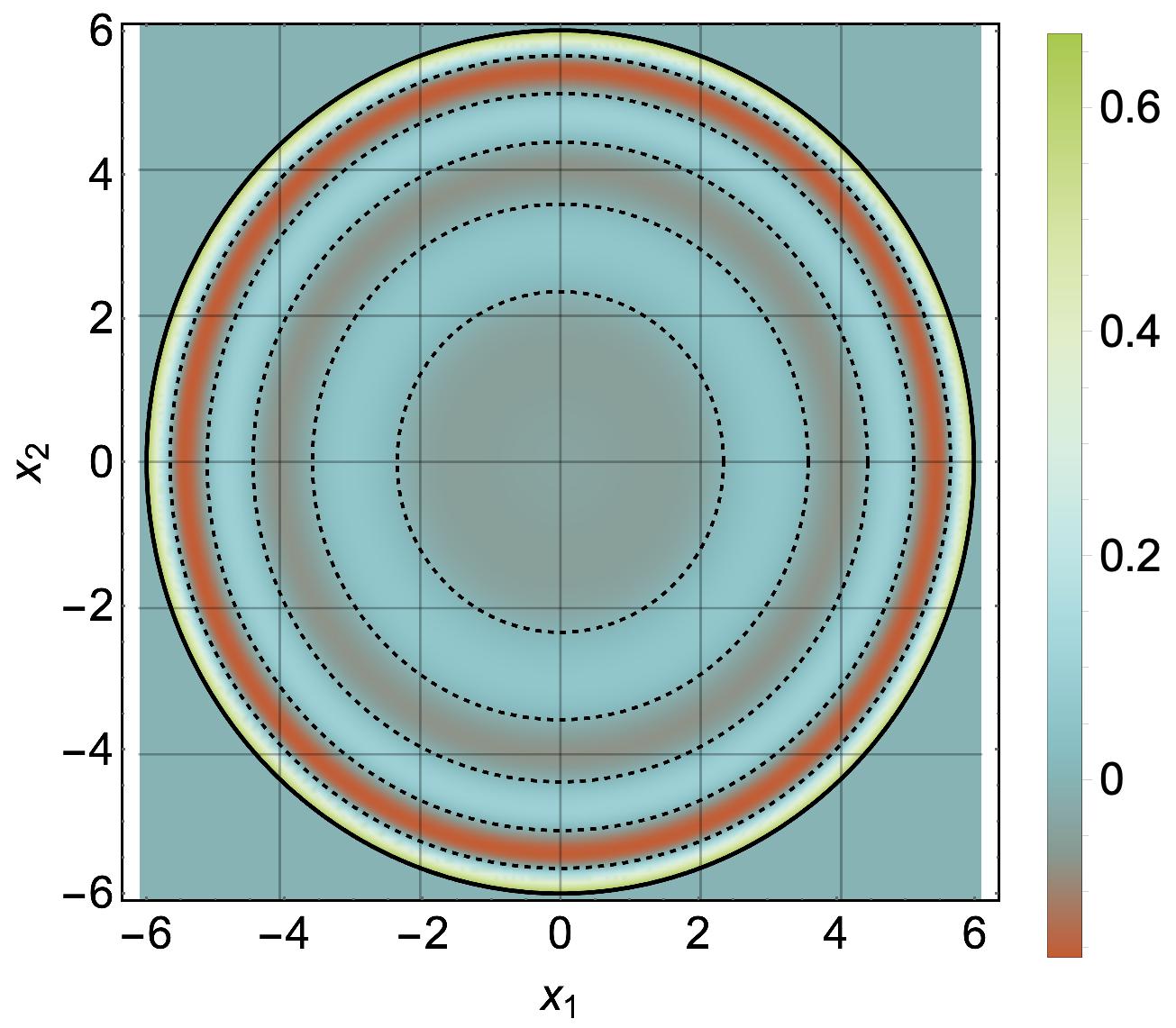
Figure 1: Partial solutions $W_{k}(z)$ (a) and the shock wave at $t=6.0$ (b).

II.3.2 Shock wave energy in (2+1) dimensions

In (2+1) dimensions, the expressions for $W_{k}(t)$ are supplied by (II.20) and (II.19), respectively, while the equation for $W^{\prime}_{k}(z)$ is given by

$$W^{\prime}_{0}(z) =\dfrac{2}{3}$$ (II.32)

$$W^{\prime}_{k}(z) =(-1)^{k}\left(\dfrac{2}{3}+\dfrac{b_{k}}{2(-z)^{3/2}}\right),\qquad k=1,2,\ldots.$$ (II.33)

The sum

$$E(t)=2\pi\Big{[}\int_{0}^{c_{i-1}}dr\;r\,H_{i}(t,r)+\sum_{k=1}^{i-1}\int_{c_{k}}^{c_{k-1}}dr\;r\,H_{k}(t,r)+\int_{c_{0}}^{t}dr\;r\,H_{0}(t,r)\Big{]}$$ (II.34)

gives the energy (II.15), where $t>2\sqrt{a_{i-1}}$. The sum (II.34) has just one term for $t<2\sqrt{a_{0}}$ (before $c_{0}(t)$ occurs)

$$E(t)=2\pi\int_{0}^{t}dr\;r\,H_{0}(t,r)=\pi t^{2}\frac{2a_{0}}{3}={\rm vol}_{2}(t)[\phi]_{z=0}.$$ (II.35)

Now we will prove that (II.34) produces an expression that is exactly similar to ${\rm vol}_{2}(t)[\phi]_{z=0}$. As a result, we write the integrals (II.34) in the following way

$$2\pi\int_{0}^{c_{i-1}}dr\;r\,H_{i}(t,r) \equiv X_{i}$$

$$2\pi\int_{c_{k}}^{c_{k-1}}dr\;r\,H_{k}(t,r) \equiv\overbrace{2\pi\int_{c_{k}}^{0}dr\;r\,H_{k}(t,r)}^{Y_{k}(t)}+\overbrace{2\pi\int_{0}^{c_{k-1}}dr\;r\,H_{k}(t,r)}^{X_{k}(t)}$$

$$2\pi\int_{c_{0}}^{t}dr\;r\,H_{0}(t,r) \equiv\overbrace{2\pi\int_{c_{0}}^{0}dr\;r\,H_{0}(t,r)}^{Y_{0}(t)}+\overbrace{2\pi\int_{0}^{t}dr\;r\,H_{0}(t,r)}^{X_{0}(t)}.$$

The sum of terms can be structured as follows

$$E(t)=X_{i}(t)+\sum_{k=0}^{i-1}\Big{(}X_{k}(t)+Y_{k}(t)\Big{)}=X_{0}(t)+\sum_{k=1}^{i}\Big{(}X_{k}(t)+Y_{k-1}(t)\Big{)}.$$ (II.36)

When the analytical form of the solution is entered into these formulas, one obtains

$$X_{0}(t) =\frac{2}{3}a_{0}\pi t^{2},$$ (II.37)

$$X_{k}(t) =\frac{\pi}{72}\frac{c_{k-1}^{2}}{a_{k-1}^{2}}\left[3b_{k}+4a_{k-1}^{3/2}\right]^{2},\qquad k=1,2,\ldots$$ (II.38)

$$Y_{k}(t) =-\frac{\pi}{72}\frac{c_{k}^{2}}{a_{k}^{2}}\left[48a_{k-1}a_{k}^{2}-32a_{k}^{3}+96b_{k}a_{k}^{3/2}-72a_{k}^{2}\frac{b_{k}}{\sqrt{a_{k-1}}}+9b_{k}^{2}\right],\qquad k=0,1,2,\ldots$$ (II.39)

The expression (II.39) can be stated in a somewhat different manner using the relations (II.23) and $\frac{b_{k}}{\sqrt{a_{k-1}}}=-\frac{2}{3}[a_{k}+\sqrt{a_{k-1}}\sqrt{a_{k}}]$ is the result of (II.25). Following some algebra, one finds

$$Y_{k}(t)= -\frac{\pi}{72}\frac{c_{k}^{2}}{a_{k}^{2}}\Big{[}3b_{k+1}+4a_{k}^{3/2}\Big{]}^{2}$$ (II.40)

$$+\frac{3\pi}{2}c_{k}^{2}\Big{[}a_{k+1}+a_{k-1}-4a_{k}+\sqrt{a_{k}}\Big{(}\sqrt{a_{k+1}}+\sqrt{a_{k-1}}\Big{)}\Big{]}.$$ (II.41)

The first term, (II.40), equals $-X_{k+1}$, whereas the second term, (II.41), is proportional to $W_{k}(-a_{k})$ and so vanishes because $z=-a_{k}$ is a zero of $W_{k}(z)$. Indeed, plugging $z=-a_{k}$ into (II.22) yields the equation

$$-a_{k}+a_{k-1}+\frac{3}{2}\frac{b_{k}}{\sqrt{a_{k}}}-\frac{3}{2}\frac{b_{k}}{\sqrt{a_{k-1}}}=0.$$

In the following, $b_{k}$ is replaced with $b_{k}+1$ by (II.23), and then $\frac{b_{k+1}}{\sqrt{a_{k}}}$ and $\frac{b_{k}}{\sqrt{a_{k-1}}}$ disappear via (II.25). It gives

$$a_{k+1}+a_{k-1}-4a_{k}+\sqrt{a_{k}}\Big{(}\sqrt{a_{k+1}}+\sqrt{a_{k-1}}\Big{)}=0.$$

This outcome demonstrates that we have the following identity

$$X_{k+1}(t)+Y_{k}(t)=0,\qquad k=0,1,2,\ldots$$ (II.42)

Finally, (II.36) gives the energy of the (2+1)-dimensional shock wave

$$E(t)=\frac{2}{3}\pi a_{0}\,t^{2}={\rm vol}_{2}(t)\,[\phi]_{z=0}$$ (II.43)

where ${\rm vol}_{2}(t)=\pi\,t^{2}$ and the discontinuity term $[\phi]_{z=0}$ is given by the (II.21) expression.

II.4 Shock waves in $3+1$ dimensions

II.4.1 Partial solutions and recurrence relations

The partial solutions that generate shock waves in $n=3$ dimensions take the following form:

$$W_{k}(z)=\frac{1}{2}(-1)^{k}z+\alpha_{k}+\frac{\beta_{k}}{z}$$ (II.44)

where $\beta_{0}=0$. A $W_{k}(-a_{k}-1)=0$ condition enables the elimination of $alpha_{k}$ yielding

$$W_{0}(z) =\frac{1}{2}(z+a_{0}),$$ (II.45)

$$W_{k}(z) =(-1)^{k}\left[\frac{1}{2}(z+a_{k-1})+b_{k}\left(\frac{1}{z}+\frac{1}{a_{k-1}}\right)\right],\ldots k=1,2,\ldots$$ (II.46)

where $\beta_{k}=(-1)^{k}b_{k}$. The partial solutions $W_{k-1}(z)$ and $W_{k}(z)$ satisfy the matching condition $W^{\prime}_{k}(-a_{k-1})=W^{\prime}_{k-1}(-a_{k-1})$ which resulting in a recurrence relation

$$b_{k}=-b_{k-1}+a^{2}_{k-1}\qquad{\rm where}\qquad b_{0}=0.$$

As a result, we obtain

$$b_{k}=-\sum_{n=0}^{k-1}(-1)^{n+k}a^{2}_{n}.$$ (II.47)

Finally, the condition $W_{k}(-a_{k})=0$ is imposed. We obtain the recurrence relation $a_{k}=\frac{2b_{k}}{a_{k-1}}$ which, when combined with (II.47), yields

$$a_{k}=\frac{2}{a_{k-1}}\sum_{n=0}^{k-1}(-1)^{n+k-1}a^{2}_{n}.$$ (II.48)

The recurrence (II.48) has a straightforward exact solution

$$a_{k}=(k+1)a_{0}.$$ (II.49)

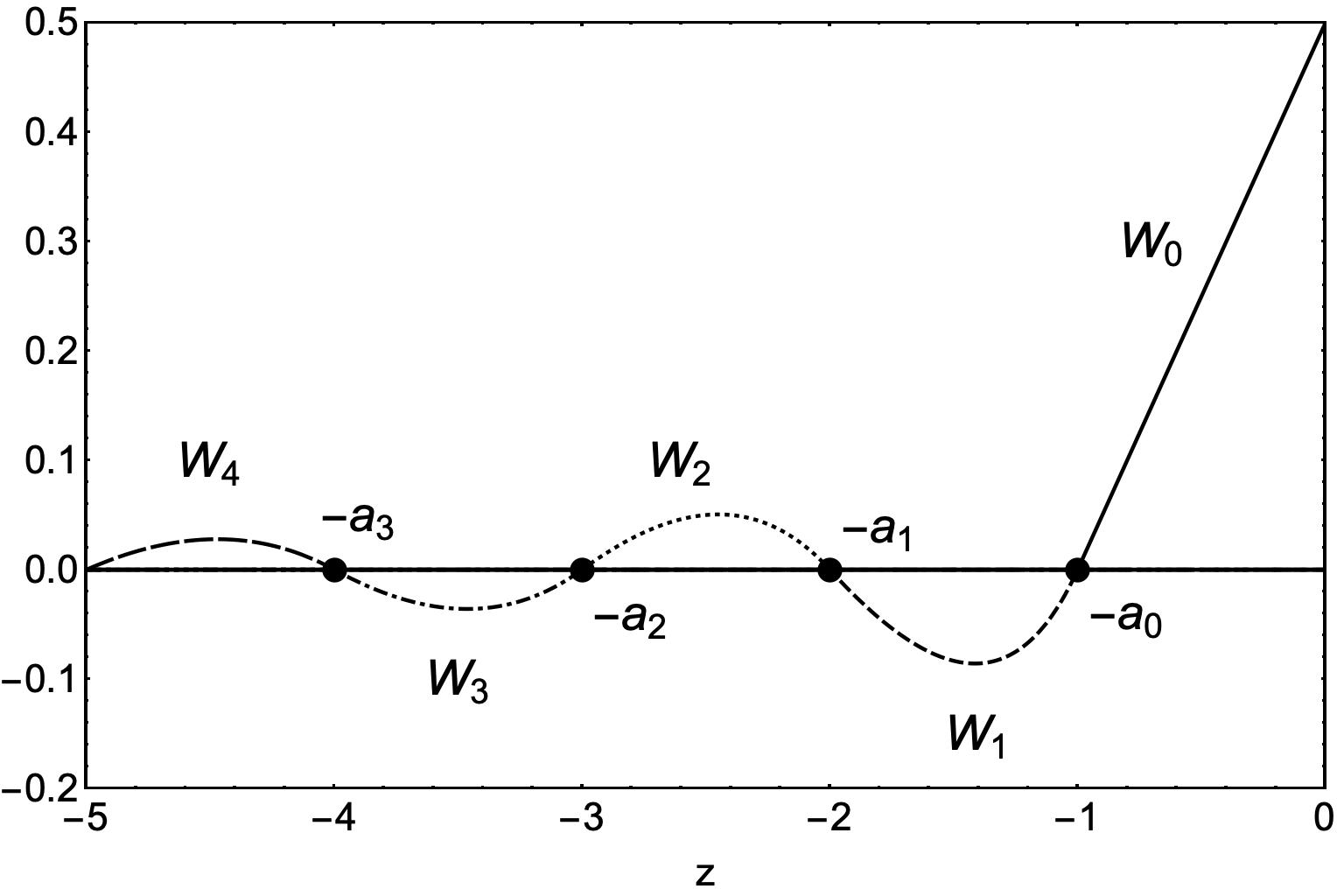
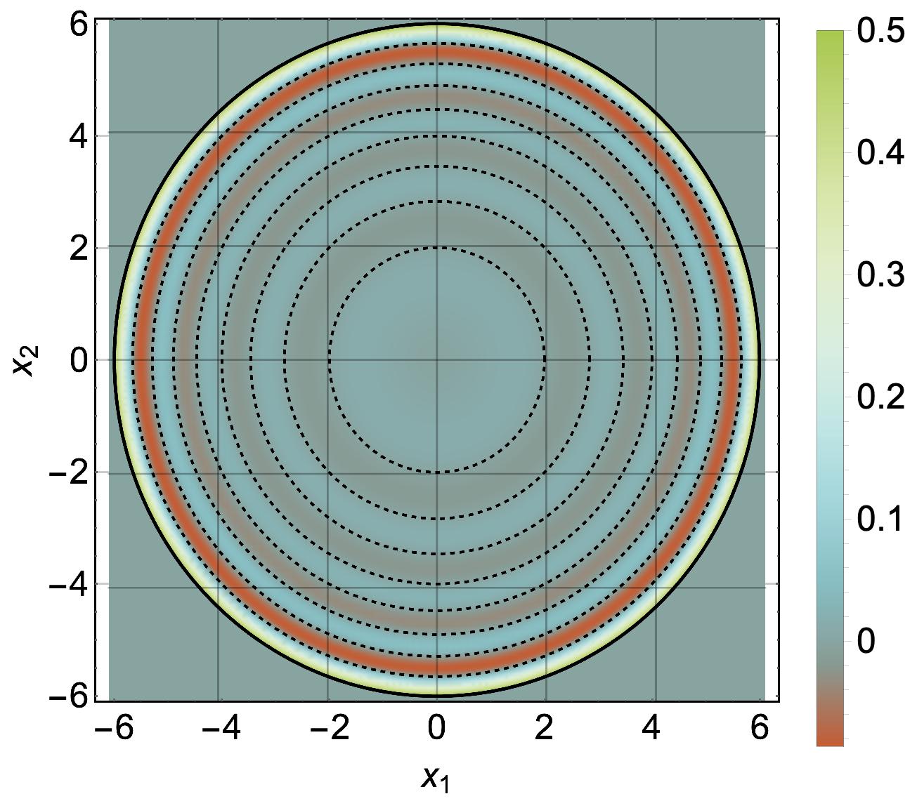
Figure 2: Partial solutions $W_{k}(z)$ (a) and the shock wave section $x^{3}=0$ at $t=6.0$ (b).

It may be verified through plugging it into (II.48) and applying the formula $\sum_{m=1}^{k}(-1)^{m+k}m^{2}=\frac{k(k+1)}{2}$. The exact form of the zeros is really useful. In particular, the explicit formulas for partial solutions (II.45) and (II.46) can be obtained.

$$W_{k}(z)=\frac{(-1)^{k}}{2z}\Big{(}z+ka_{0}\Big{)}\Big{(}z+(k+1)a_{0}\Big{)},\qquad k=0,1,2,\ldots.$$ (II.50)

We displayed a few first partial solutions $W_{k}(z)$ in Fig.2.

II.4.2 Shock wave energy in (3+1) dimensions

The energy of a shock wave in (3+1) dimensions is given by the following expression (II.36) where

$$X_{0}(t) \equiv 4\pi\int_{0}^{t}dr\;r^{2}\,H_{0}(t,r),$$ (II.51)

$$X_{k}(t) \equiv 4\pi\int_{0}^{c_{k-1}}dr\;r^{2}\,H_{k}(t,r),\qquad k=1,2,\ldots$$ (II.52)

$$Y_{k}(t) \equiv 4\pi\int_{c_{k}}^{0}dr\;r^{2}\,H_{k}(t,r),\qquad k=0,1,2,\ldots.$$ (II.53)

which is similar to the preceding example.

(II.50) gives the expression $W_{k}(z)$, whereas $W^{\prime}_{k}(z)$ takes the form

$$W^{\prime}_{k}(z)=\frac{(-1)^{k}}{2z^{2}}\Big{(}z^{2}-k(k+1)a_{0}^{2}\Big{)}.$$ (II.54)

Plugging these formulas into (II.51), (II.52) and (II.53) yields

$$X_{0}(t) =4\pi\left(\frac{a_{0}}{6}t^{3}\right),$$ (II.55)

$$X_{k}(t) =4\pi\left(\frac{a_{0}}{24k}c_{k-1}^{3}(t)\right), k=1,2,\ldots$$ (II.56)

$$Y_{k}(t) =4\pi\left(-\frac{a_{0}}{24(k+1)}c_{k}^{3}(t)\right), k=0,1,2,\ldots.$$ (II.57)

It follows from (II.56) and (II.57) that $X_{k}(t)=-Y_{k-1}(t)$ and thus the energy (II.36) in $(3+1)$ dimensions simplifies to the formula $E(t)=X_{0}(t)$, which is true for any $t$. We conclude that the wave energy inside the light cone grows as a third power of time. The discontinuity of the field at the light cone in three spatial dimensions is given by

$$[\phi]_{z=0}=\lim_{z\rightarrow 0-}W_{0}(z)=\frac{a_{0}}{2}.$$ (II.58)

By denoting a volume of the sphere occupied by the wave with ${\rm vol_{3}}(t):=\frac{4\pi}{3}t^{3}$, we find that the energy of the wave is given by a product of the volume of the sphere and the magnitude of discontinuity. This energy manifests itself as

$$E(t)={\rm vol}_{3}(t)[\phi]_{z=0}.$$ (II.59)

II.5 Numerical solution of a non-homogeneous equation

We argued in Section (II) that a solution with propagating and fixed discontinuity at the light-cone solves the ordinary differential equation with the Dirac’s delta force $F(\phi(z))=C_{n}\delta(z)$, where $F(\phi)$ is supplied by (II.8) and $C_{n}=\frac{n-1}{2}W(0)$. This solution is provided by (II.7), which contains the Heaviside step function. The goal of this section is to obtain a numerical approximation of the solution $\phi(z)$ as a result of the Dirac’s delta force $\delta(z)$.

To be more didactic before proceeding to the problem, we briefly review a well-known result for a harmonic oscillator. The fundamental solutions for a harmonic oscillator are functions that satisfy the following equation $D^{\prime\prime}(t)+\omega^{2}D(t)=\delta(t)$. There are two types of solutions: retarded $D_{R}(t)=\theta(t)\frac{\sin(\omega t)}{\omega}$ and advanced $D_{A}(t)=-\theta(-t)\frac{\sin(\omega t)}{\omega}$. To obtain numerical solutions, we must substitute the Dirac’s delta with its regularized approximation:

$$\delta_{\epsilon}(t)=\frac{1}{\sqrt{2\pi\epsilon}}e^{-\frac{t^{2}}{2\epsilon}}$$ (II.60)

which tends to $\delta(t)$ as $\epsilon$ tends to zero. To obtain a retarded solution, we select initial conditions at $t_{0}$: $D(t_{0})=0$ and $D^{\prime}(t_{0})=0$, and then solve the equation for $t\geq t_{0}$. The outcome is shown in Fig.3, where we choose $t_{0}=-2$, $\omega=2$, and $\epsilon=0.005$. We also plotted the regularized delta divided by factor 10 to avoid changing the scale of the image. Figure 3 shows a similar result for $D_{A}(t)$ for $t_{0}=2.0$. The given result demonstrates that the system receives energy within a limited interval around $t=0$, causing oscillations. Out of this interval, the force is practically nil, and oscillations are regulated by the same homogeneous equation that governs the case of a nontrivial initial condition.

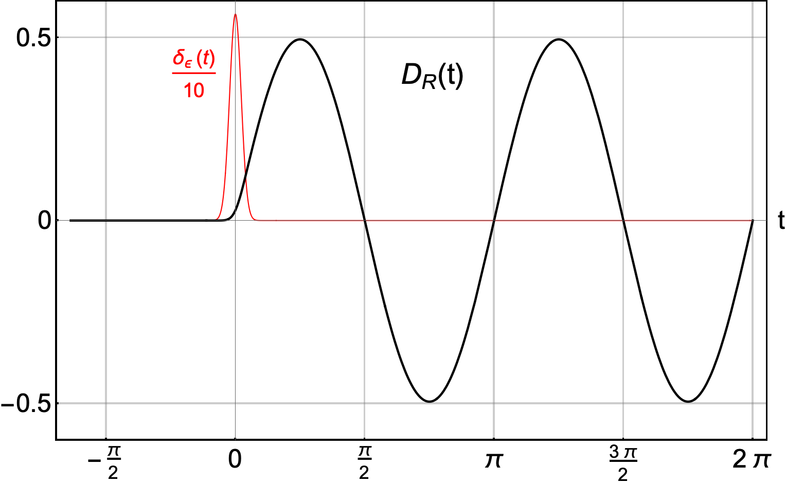
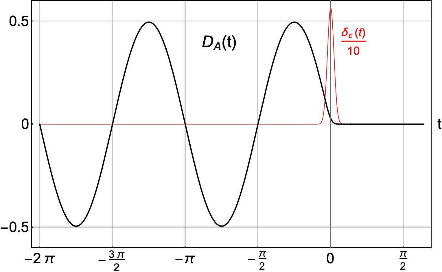
Figure 3: Fundamental harmonic oscillator numerical solutions: (a) retarded solution $D_{R}(t)$ and (b) advanced solution $D_{A}(t)$ for $\epsilon=0.005$. In both figures, the regularized delta force $\delta_{\epsilon}(t)$ is divided by 10.

Now we return to the subject of shock waves. The main difference in the shock wave problem is that the variable $z$ is not a time, and so delta force does not act at a single instant of time, but is present constantly at the surface of the light cone. It signifies that the system is continuously getting energy. The exact solution’s form $\phi=\theta(-z)W(z)$ suggests that we take the ”initial” condition $\phi(z_{0})=0$, $\phi^{\prime}(z_{0})=0$ at some $z_{0}>0$ and numerically solve the equation for $z\leq z_{0}$. However, finding a solution is not easy since there is an obstacle at $z=0$, which is related with unlimited growth of $\phi(z)$ and its derivative. From an analytical standpoint, as shown in (II.12) and (II.13), the equation (II.11) comprises solutions with singular expressions $\ln(-z)$, ${(-z)^{-1/2}}$, and $(-z)^{-1}$ in $1+1$, $2+1$, and $3+1$ dimensions, respectively. These expressions have been eliminated from $W_{0}(z)$ by using the free parameter $\beta_{0}=0$. As a result, the partial solutions around $z=0$ are linear functions, i.e. $W^{\prime\prime}_{0}=0$. It implies that by restricting the numerical analysis to the vicinity of the point $z=0$, the troublesome term containing the second derivative can be eliminated. This step must be handled with caution. Let us divide (II.8) into two expressions: $F(\phi)=F_{2}(\phi)+F_{1}(\phi)$, where $F_{2}(\phi)=-z\phi^{\prime\prime}$ and $F_{1}(\phi)=-\frac{n+1}{2}\phi^{\prime}+{\rm sgn}(\phi)$. Because the second derivative term acting on a function $\theta(-z)W(z)$ yields the Dirac’s delta term

$$F_{2}(\theta(-z)W(z))=-W(0)\delta(z)-\theta(-z)zW^{\prime\prime}(z)$$

the coefficient multiplying delta force on the right hand side of the equation must be changed simultaneously. We can observe that $F_{1}(\phi)$ evaluated on $\theta(-z)W(z)$ yields

$$F_{1}(\theta(-z)W(z))=\frac{n+1}{2}W(0)\delta(z)+\theta(-z)\Big{[}-\frac{n+1}{2}W^{\prime}(z)+{\rm sgn}(W)\Big{]}.$$

It indicates that replacing $F(\phi)$ with $F_{1}(\phi)$ on the left side of the equation $F(\phi)=\frac{n-1}{2}W(0)\delta(z)$ implies replacing the coefficient $\frac{n-1}{2}$ with $\frac{n+1}{2}$ on the right side. As a result, we have the equation

$$-\frac{n+1}{2}\phi^{\prime}+{\rm sgn}(\phi)=\frac{n+1}{2}W(0)\delta(z)$$ (II.61)

in vicinity of $z=0$. It is worth noting that this approach demonstrates that even when $n=1$, we end up with a nonhomogeneous equation near to $z=0$, implying that we can obtain a nontrivial solution for $\phi(z_{0})=0$ as well as $\phi^{\prime}(z_{0})=0$. It also implies that our strategy is correct. In what follows, we solve numerically equation (II.61) with $W(0)$ as a free parameter and (II.60) to replace the precise Dirac’s delta distribution.

We consider the case $n=2$. First we chose a point outside the light cone $z_{0}=0.3$ and take the initial conditions $\phi(z_{0})=0$ and $\phi^{\prime}(z_{0})$. In the absence of the delta force, the only solution to the equation (II.61) with such initial conditions would be zero. For regularized delta force, we use $\epsilon=10^{-6}$ and fix a free parameter $W(0)=\frac{2}{3}$. Then we numerically solve equation (II.61) on the symmetric interval $-z_{0}\leq z\leq z_{0}$.

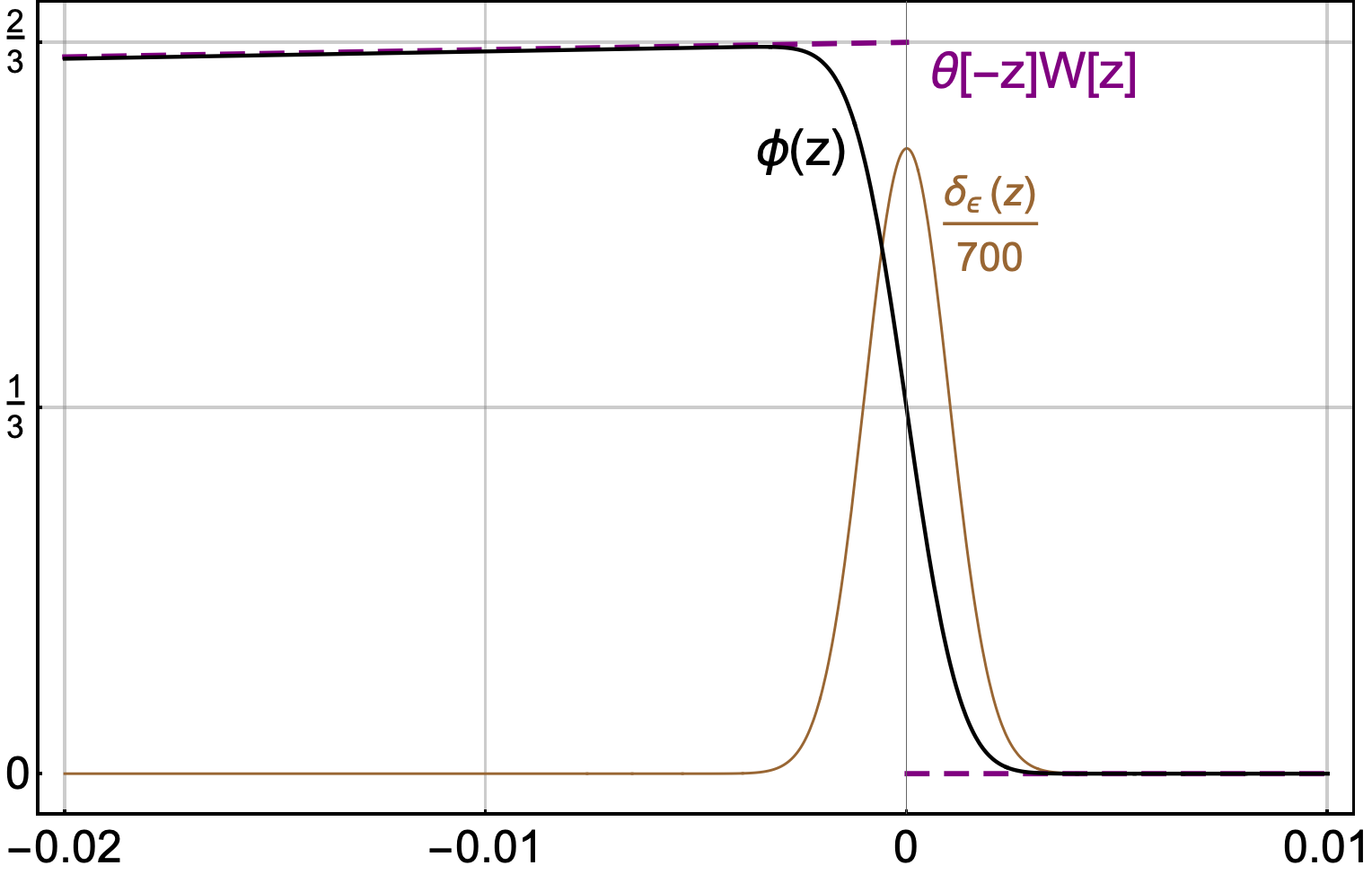
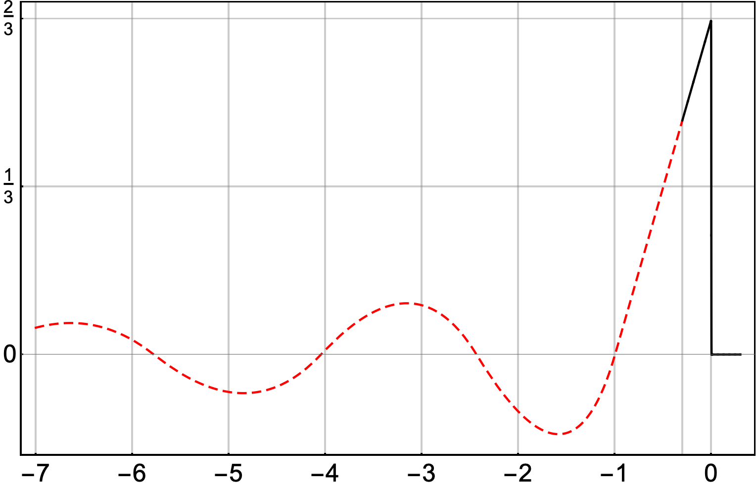
Figure 4: Numerical solution $\phi(z)$ of (II.9) for $n=2$, $W(0)=\frac{2}{3}$ and $\delta(z)\approx\delta_{\epsilon}(z)$ where $\epsilon=10^{-6}$. (a) an enlarged image of a solution close to $z=0$, and (b) a complete solution achieved by first solving (II.61) and then (II.9). The matching point is chosen as $z_{m}=-0.3$.

Figure 4 depicts only a tiny element of this solution. We have also displayed a delta force to indicate the region where it is relevant. To keep the plot’s scale, the delta $\delta_{\epsilon}(z)$ was shown after being divided by some arbitrary factor. We also plot a piece of the $\theta(-z)W_{0}(z)$ solution to compare it to a numerical solution. In a tiny region about $z=0$, when delta force is significantly different from zero, the numerical solution exhibits nonlinear behavior. It fast approaches the analytical partial solution $W_{0}=\frac{2}{3}(z+1)$, which is denoted by a dashed line. In Fig.4, we additionally depict a part of a numerical curve at $z<-z_{0}$, which requires solving the whole equation (II.9). We use as the initial data $\phi(-z_{0})$ and $\phi^{\prime}(-z_{0})$ given by solution of (II.61). The red dashed curve denotes the second part of the curve. As can be seen, the numerical solution closely approximates the actual answer shown in Fig.1. It is straightforward to show numerically that a different choice of a free parameter $W(0)$ that multiplies the delta force allows for the achievement of the required maximum (discontinuity in the exact solution) at the light cone. We will skip the other cases and go to a more in-depth investigation based on the numerical solution of a homogeneous PDE equation. In this work, we will examine mimicking the influence of delta force through explicit implementation of boundary conditions.

II.6 Generalization of energy expression

In this section we propose that expression (II.18) can, as might seem intuitive by its very simple form, be generalized to arbitrary positive integer values of $n$. Equation (II.9) already suggests that, because $W(0)$ is a free parameter, a solution theoretically similar to the analytic shock waves can be obtained by using $\phi(t,r)|_{z}=0={\rm const}$ as a Dirichlet boundary condition. That has been demonstrated by special treatment of the region $z\simeq 0$, which leads to equation (II.61) and then its validation via numerical regularization and integration of the delta distribution.

Given that $\phi(t,r)|_{z}=0$ is fixed and that the system conserves energy in all other regions of space, we can generalise energy expression of the system. Instead of suddently raising the value of the field to $W(0)$, we now consider that the whole field (to spatial infinity) is raised to that value (see Fig. 5), and that inside the light cone of the event $(t,r)=(0,0)$, we release the field to allow its dynamic. Now, because when the field is released from region (both in time and space) where it is flat, it has all its partial derivates set to null (including its time derivative), then no gradient or kinetic energy is forced in the field, leaving only the “gravitational” energy term $V[\phi(t,r)]_{z=0}=|W(0)|$ as a source (one possible mechanical representation of the system in 2+1 dimensions is an elastic membrane in a gravitational field over a rigid plane). As the field is released, of course, this potential energy is converted to kinetic and gradient energy according to the $n$-dimensional SG equation. However, no new energy was introduced outside that from $|W(0)|$ at this point, implying that all additional energy is derived from the released potential energy. When this heuristic is used to illustrate how energy is poured into the future light cone of the $(0,0)$ event, it becomes evident that the amount of energy inside it is its (hyper) space integral, weighted by the potential of the previous value of the field. In other words, it is the length of a light cone time slice multiplied by $|W(0)|$. This measure is the area/volume/hipervolume/etc. of the disc/sphere/hipersphere/etc. contained inside the future light cone at a time $t$, already presented in this paper as ${\rm vol}_{n}(t)$. Also, in this context, the $|W(0)|$ term is no different than the field discontinuity $[\phi]_{z=0}$, which, together with ${\rm vol}_{n}(t)$ reproduce, for arbitrary $n$, the expression (II.18).

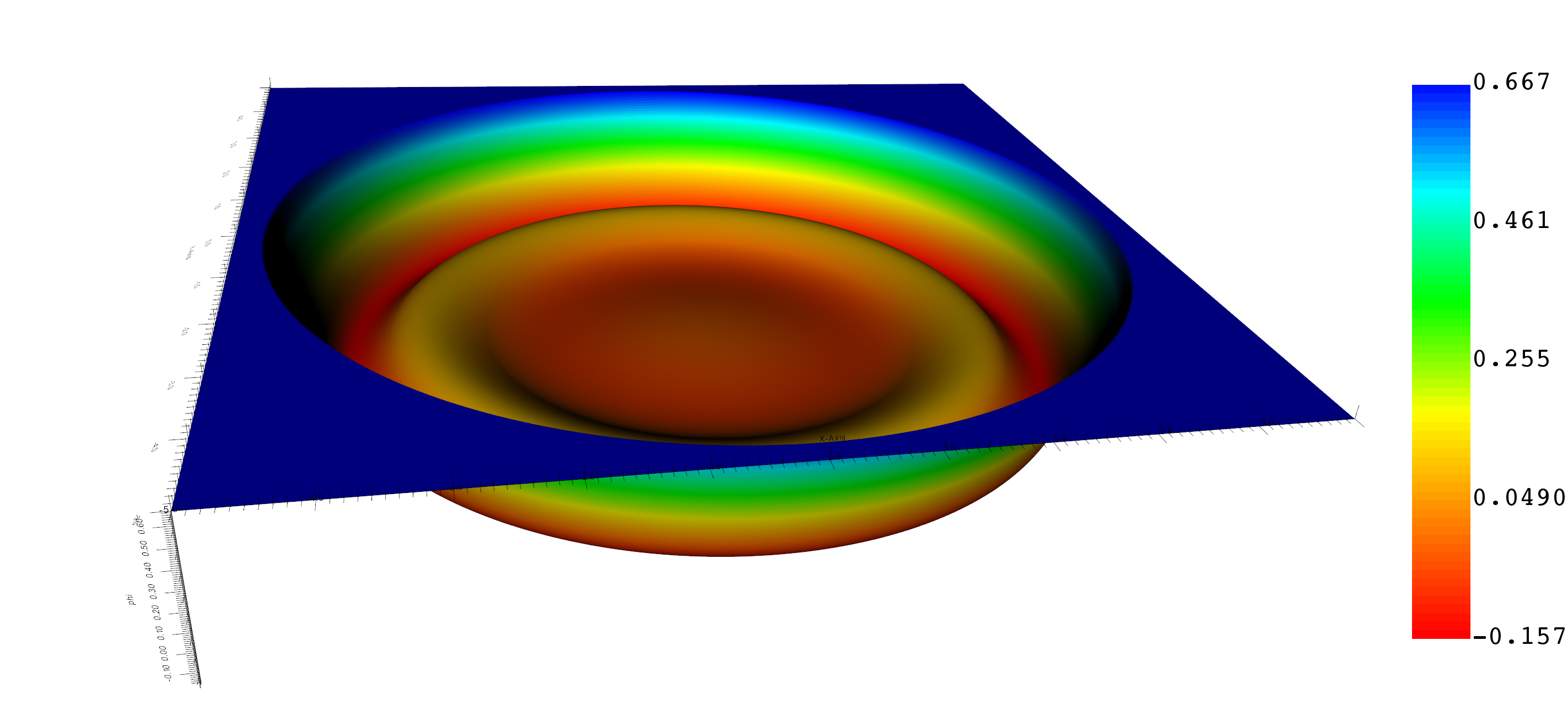
Figure 5: The whole field starting from value $W(0)=2/3$ (the plateau visible in the image), and its dynamic being allowed to happen within the light-cone of event $(t,r)=(0,0)$.

III Numeric evolution of shock waves

III.1 General remarks

This section demonstrates numerically how shock-waves in $(2+1)$ dimensions develop. The exact solutions do not conserve energy, as shown in sections (II.2), (II.3.2) and (II.4.2), i.e. the energy of the solution inside the light cone expands with time (see (II.18)). In other words, the exact solution occurs if there is continuous energy transfer into the region within the light cone where the solution assumes its nontrivial form. The increase has its origins in the limitless reservoir of gradient energy carried by the discontinuity of the field at the wave front (at the border of its light-cone) in one spatial dimension, $n=1$. The wave’s profile function $W(z)$ is a solution of the homogeneous second order differential equation (it lacks the leading-delta term).

To obtain shock waves in higher dimensions ($n>1$) that are similar to one-dimensional shock waves, an additional non-homogeneous term must be included in the field equation. The Dirac’s delta term is proportional to this term. It follows that the existence of such waves necessitates the presence of a $\delta$-force, the support for which is concentrated at the light cone $z=0$ (see (II.9)). As a result, solutions $\phi(z)=\theta(-z)W(z)$ can have a stable value at $z=0$, i.e. $\lim_{z\rightarrow 0-}\phi(z)=a_{0}$. In (II.3) and (II.4), the exact form of such solutions has been obtained. In the previous subsection (II.5), we addressed the difficulty of numerically solving a nonhomoheneous ODE equation, and we learnt that there are technical problems with numerically solving the equation in the vicinity of the light cone due to the $-z\phi^{\prime\prime}$ element in the equation. We do not expect this problem to disappear when we apply the full 2+1 solution on discretized spacetime. As a result, we will solve numerically the PDE homogeneous equation while explicitly applying the Dirichlet condition at the light cone $\lim_{r\rightarrow t-}\phi(t,\vec{x})=W(0)$. The boundary condition mimics the effect of the Dirac’s delta force in such an approach. The whole time dependent simulation allows us to investigate the issue of shock wave desintegration after turning off the external source of energy at some point. This is accomplished by switching the boundary condition at some point in time.

The integrations are performed using the standard explicit Runge-Kutta method, with 4${}^{\text{th}}$ order time oversampling (explicit RK4). Field state is a typical numeric double-precision representation of space dispersed over a rectangular mesh discretized representation. The field region is a square with side length $L$ that was chosen as a subset of the simultaneity surface whose center coincides with the shock wave’s in its frame of reference. It is divided into an integer number $N$ of discrete cells in each direction, defining the area $h^{2}$ of each mesh site such that $h=L/N$, for a total of $N^{2}$ cells forming the representation. The entire distribution is advanced through an RK4 step to obtain incremental advances of field state from time $t$ to time $t+\delta t$. The fixed timestep is specified, as is the fixed value $\delta t=h/10$.

The differential Laplace operator is represented by a matrix, and it is computed over the space mesh using a convolution with the kernel shown below

$$[\Delta^{2}]_{kern}=\dfrac{1}{h^{2}}\begin{bmatrix}0\quad&1\quad&0\\ 1\quad&-4\quad&1\\ 0\quad&1\quad&0\end{bmatrix}.$$ (III.1)

It is worth noting that neither the square form of space nor its mesh is discretized in the most appropriate representation for radially-symmetric solutions. This permits an isotropic analytic (continuous) input (the boundary conditions) to evolve in an anisotropic (and discontinuous) numerical space – which is theoretically isotropic in the limit $N\rightarrow\infty$ – resulting in a break in the input’s radial symmetry. This split reflects numerical error accumulation and is used as a measure of simulation validity. In our scenario, the contour of the space is ignored: once the border is reached by a non-vacuum field, we consider the simulation to have reached its maximum time. With this in mind, we show our reference simulation for a shock wave with discontinuity $W(0)=2/3$ up to time $t=7.5$ in Fig. 6.

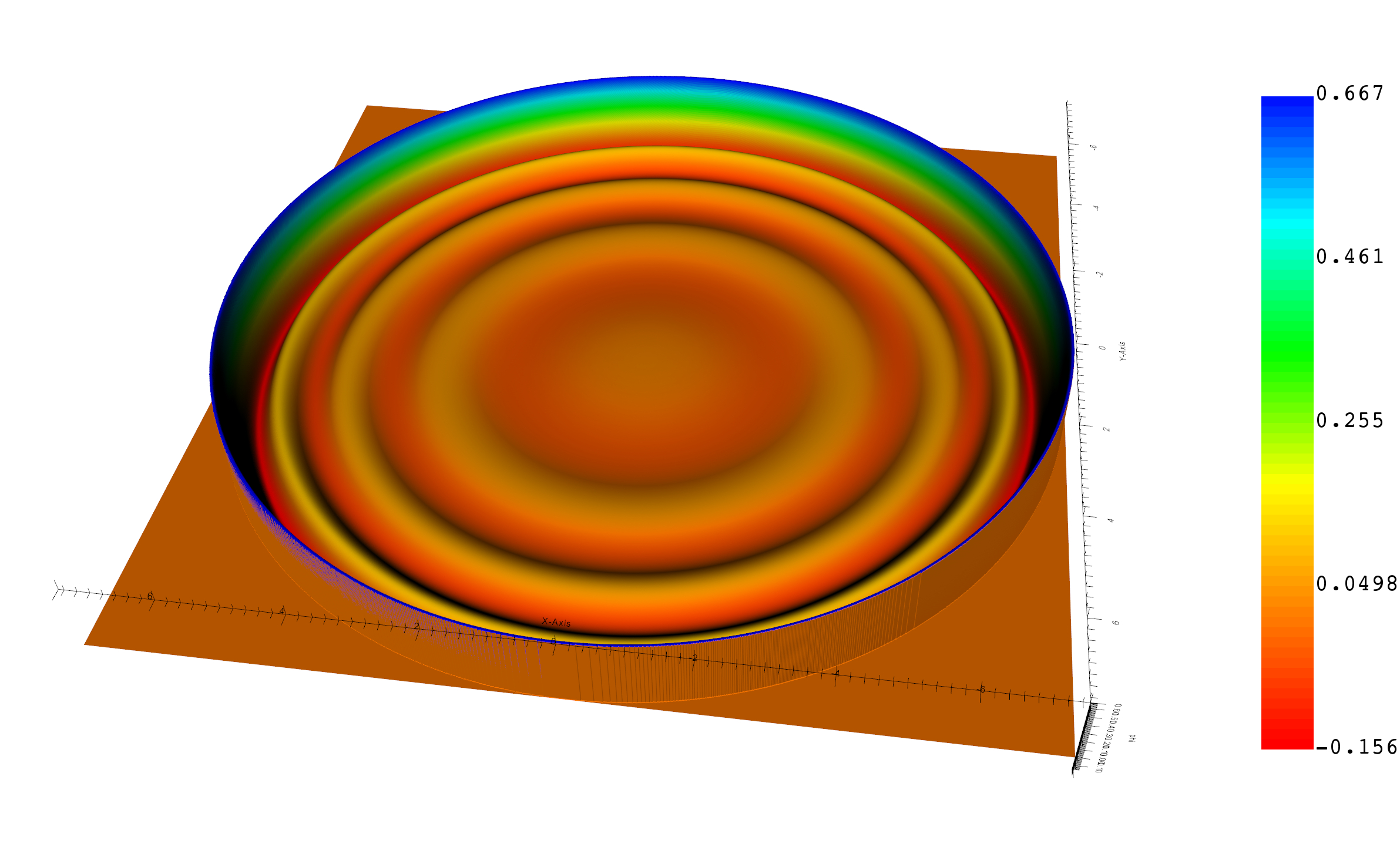
Figure 6: Our reference shock wave simulation. The numeric space discretization has different symmetry than the analytic solution. The fact it has not sensibly affected the simulation is indicative of little or no accumulation of error. Colorbar indicates field value, as does height.

III.2 Shock wave solution for the Dirichlet boundary condition

We solve the equation (II.1) in the region $r<t$ using the Dirichlet boundary condition at the light cone’s surface $\phi(t,r=t)=const$. The imposed Dirichlet condition expresses the class of solutions addressed here, which is represented by the ansatz (II.7). The simulation region is limited to $r<t$, whereas the surface at the light cone and the field outside of it are explicitly fixed as

$$\phi(t,\vec{x})=\left\{\begin{array}[]{ccc}W(0)&{\rm for}&r=t\\ 0&{\rm for}&r>t\end{array}\right..$$ (III.4)

In Fig.7 we plot the section of a shock wave profile along the axis $x$ at $t=7.25$. Its time derivative is shown in Fig.7. These are sections of the wave presented in Fig. 6. The actual shock wave solution was superimposed to verify our numerical result.

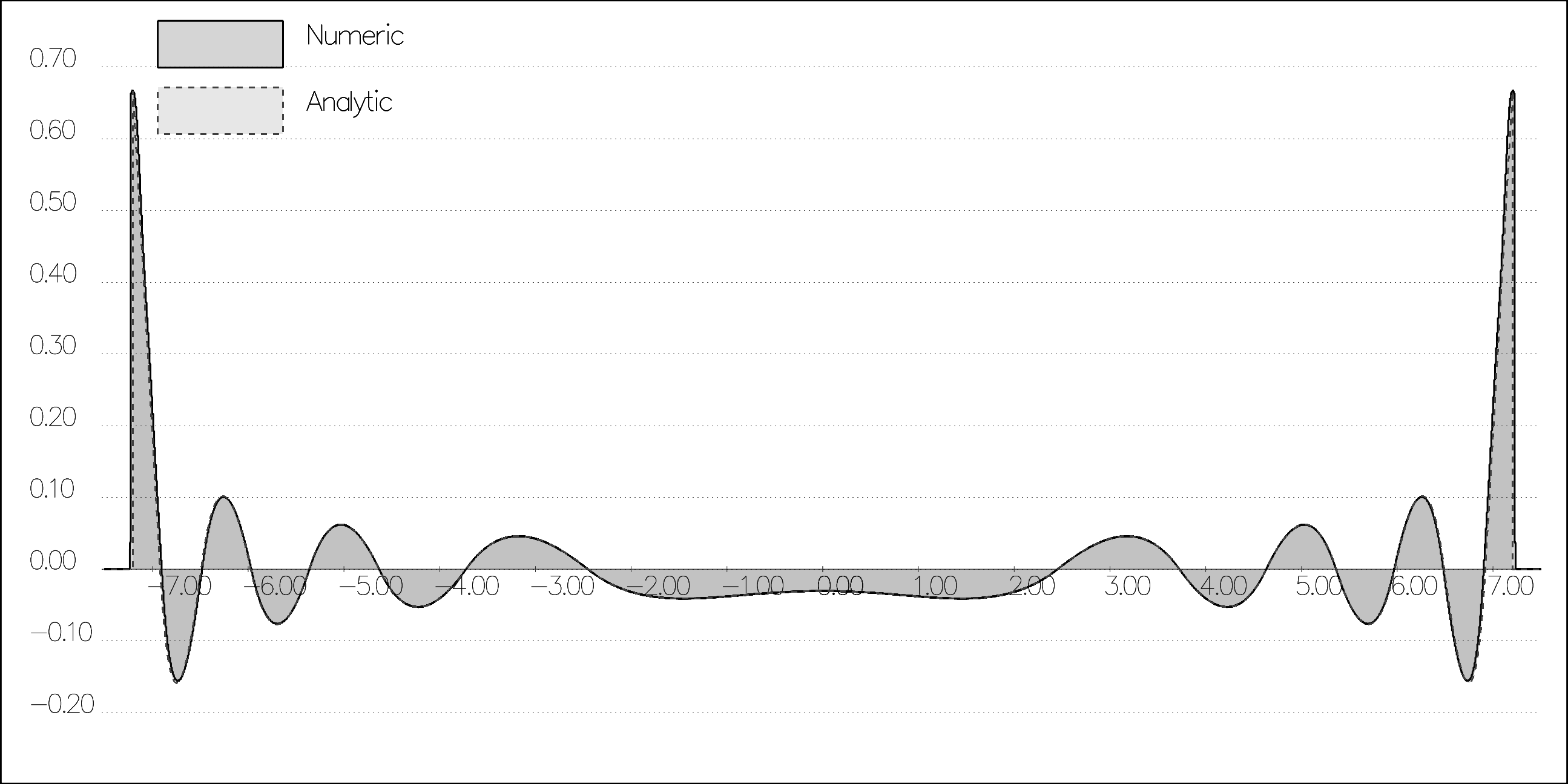
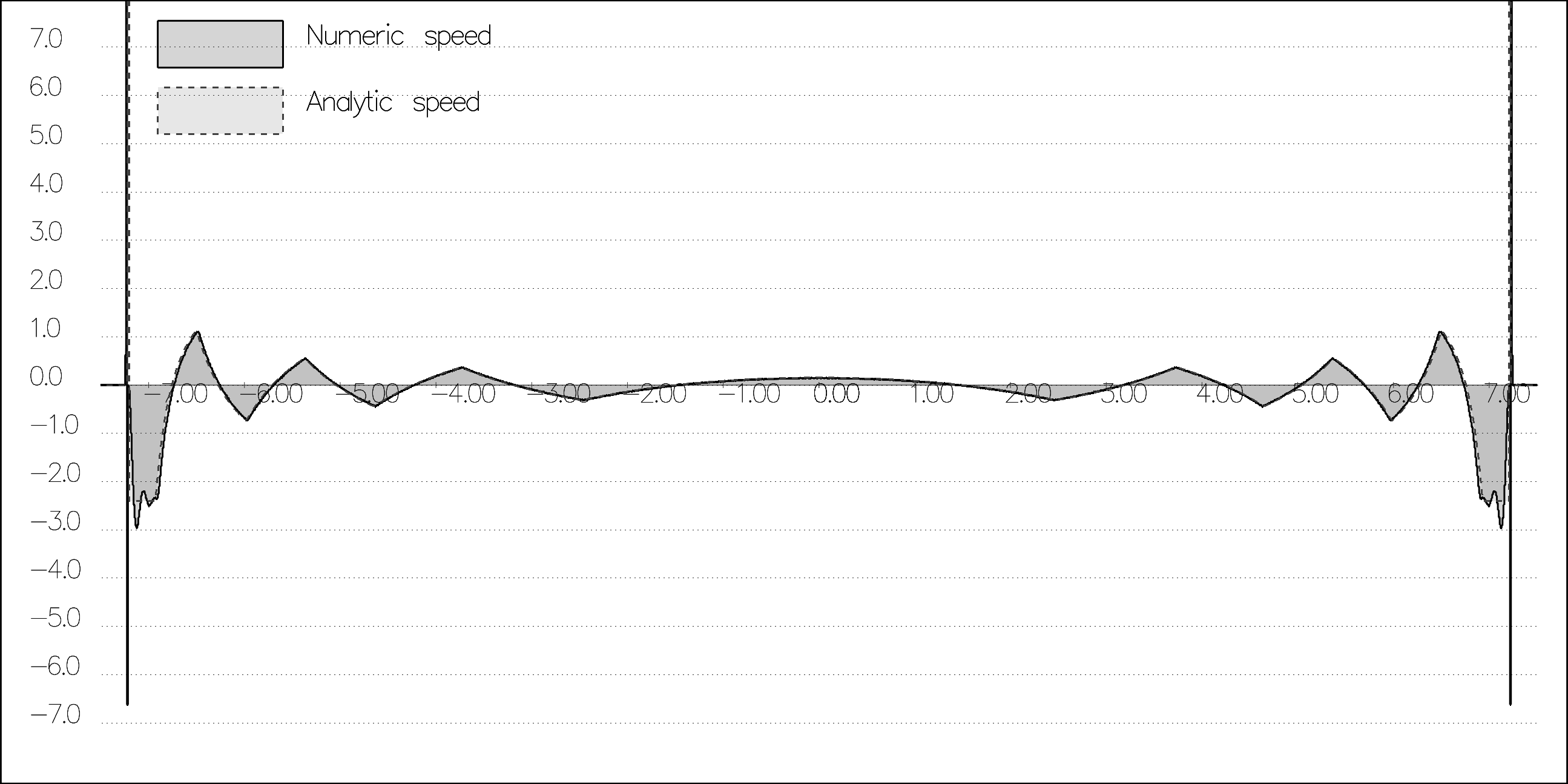
Figure 7: The numerically obtained shock wave section $y=0$, $t=7.25$ and the actual shock wave solution (a) and their time derivative (b).

Figure 8 depicts the evolution of the solution in a spacetime diagrams of the shock wave with the value of the scalar field indicated by a gradient color. The section depicted lies in the $tx$-plane. Fig.8 shows the time evolution of the ratio between the numeric solution and the analytic solution.

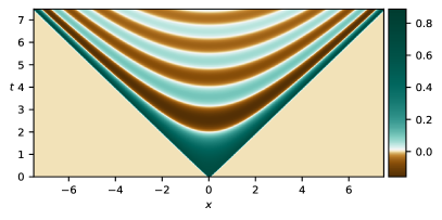
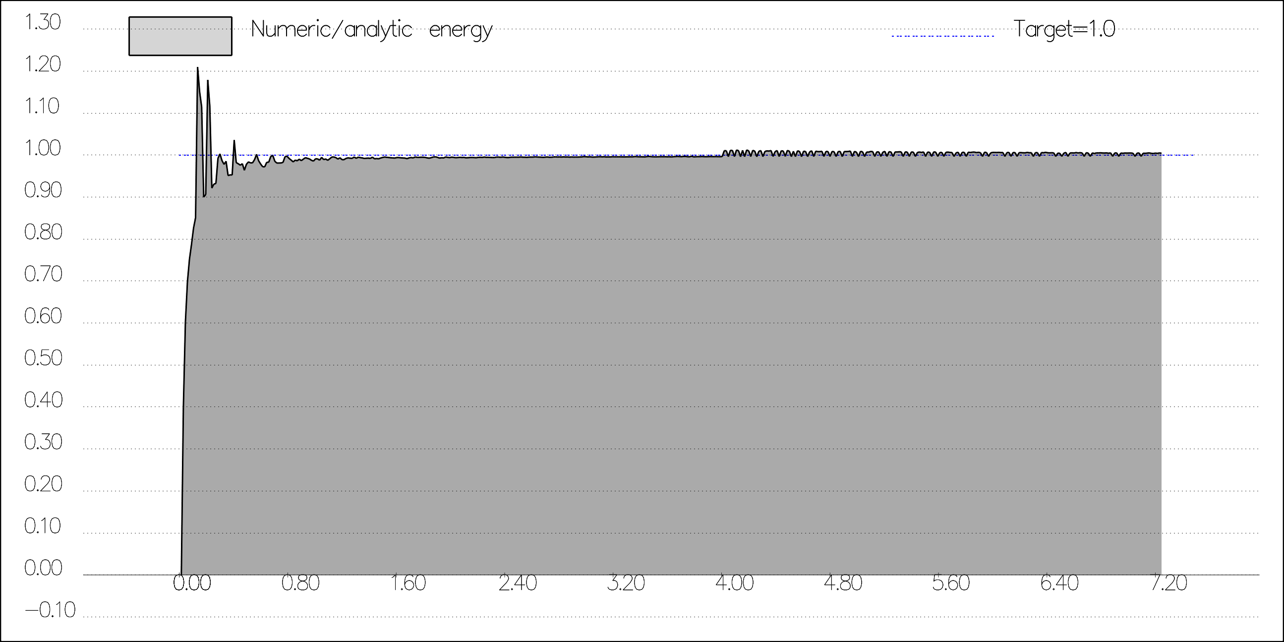
Figure 8: Section $tx$ of the shock wave solution’s gradient color spacetime portions in $n=2$ spatial dimensions (a) and the ratio between numeric and analytic energy inside the shock wave (b). Spikes at the beggining of energy ratio are due to numerical errors while including or not discrete square sites in disc energy integration.

III.3 Shock wave disintegration

In this section, we will look at the following issue. We consider a shock wave produced by the evolution of the scalar field $\phi$ in the interval $0<t<t_{0}$ with the constraint (III.4). The condition is turned off at $t=t_{0}$, which is analogous to the elimination of the delta force in a nonhomogeneous equation. Switching off the source means that the process of transferring energy to the shock wave has been physically disturbed, and the wave can no longer propagate in line with analytical calculations. A close-up of the history of section $tx$ of the field is shown in Fig. 9. This is a zoom in on the lower central part of Fig. 10(a). It demonstrates that the shock wave is unaffected inside the region formed by the intersection of the interior of the event’s future light cone $(0,0)$ and the event’s past light cone $(2t_{0},0)$.

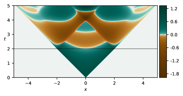
Figure 9: Initial stages of shock wave degradement. The condition (III.4) is released when $t=2.00$ is reached (black horizontal line). The red diagonal lines separate the interface between delta-driven solution vs. delta turned off. Note these red lines come in close, parallel pairs. The pair separation is $2\epsilon$, being a reference to the compact regularized delta $\epsilon$ parameter.

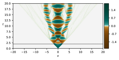
(a)  Section $tx$ of $(2+1)$ dimensional Minkowski diagram

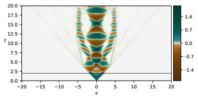
(b)  Section with $22.5\deg$ ($\pi/8$) rotation from that of (a)

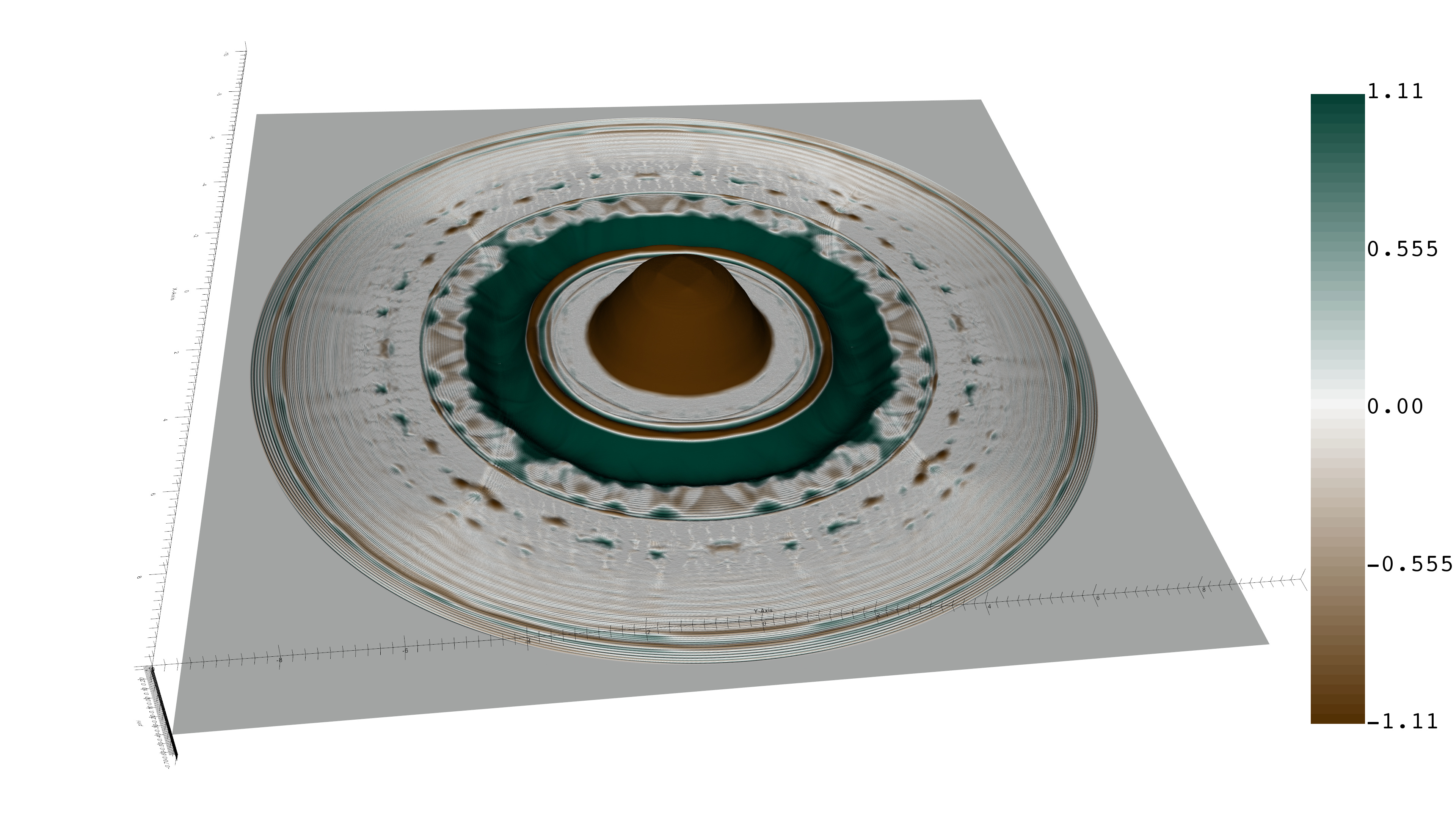
(c)  Intermediate snapshot of the center of the field at $t=10$, with side $L=10$

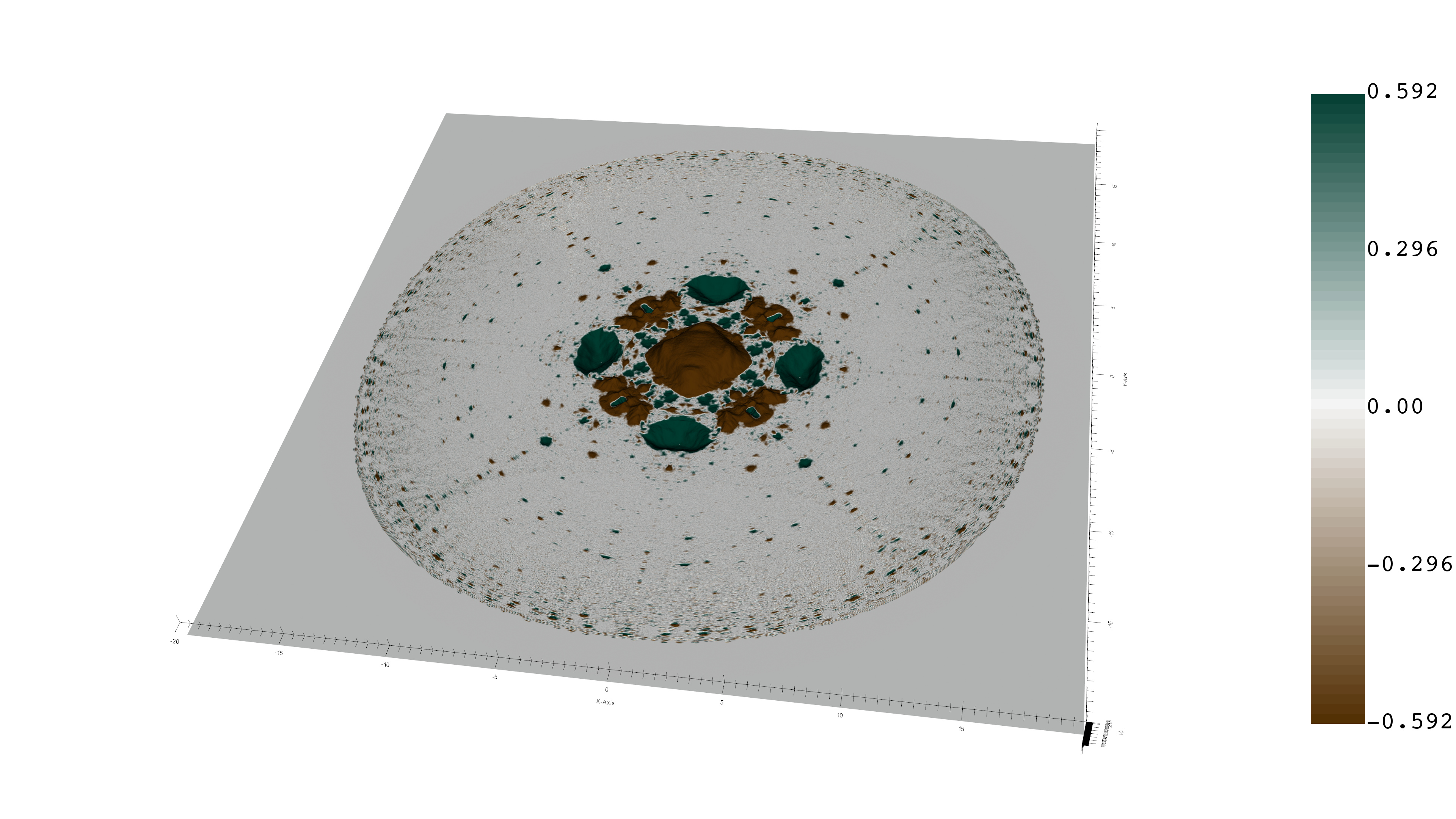
(d)  The final full field configuration, at $t=20$, showing all simulation region with side $L=20$

Figure 10: Shock wave degradement. The condition (III.4) is released when $t=2.00$ (black horizontal line in (a) and (b)) is reached. The red diagonal lines separate the interface between delta-driven solution vs. delta turned off. Spacial snapshots from $t=10$ (c) and $t=20$ (d). Note the broken isotropy of the field in (d).

Fig. 10 shows one such example. The $y=0$ plane of the $(2+1)$ Minkowski space is shown in Fig. 10(a) (the history of the $y=0$ section of the field), while Fig. 10(b) shows a $\pi/8$ angle from that, or the $y=x/2$ plane. Fig. 10(c) shows a zoom to the central part of the $t=10$ plane (a snapshot of the mid instant of the simulation). Fig. 10(d) shows a snapshot of the final, full field configuration, at $t=20$.

We would like to point to the fact that, like in $n=1$ from Hahne et al. (2020b), compact structures emerge on the field. In the current case ($n=2$), though, not only structures similar to the analytic oscillon arise (central bump), but also a novel ring formation just outside of this oscillon-like structure. While Figs. 10(a) and 10(b) show these structures to have consistency in time, Figs. 10(c) and 10(d) show their actual shape, indicating the central oscillating structure is indeed stable, while the compact ring is broken into several smaller oscillating structures.

Although this break in rotation symmetry is caused by numerical errors that give rise to high frequency oscillating modes of the field, we feel it does not invalidate the essential observation of ring emergence instability and center oscillon stability. On the contrary, it serves as strong perturbation that further indicate important properties of these structures. The main larger structures in Fig. 10(c) at $t=10$ (the central oscillon-like bump and its surrounding compact ring) have not broken this symmetry, except for some added noise. This indicates that these structures indeed are consistent channels for decay/thermalization of the $2+1$ dimensional SG shock wave.

IV Conclusions and remarks

In this study, we looked at a specific class of SG equation solutions with a discontinuity near the light cone. Such solutions were previously only known in the case of a single spatial dimension. We verified that using the same ansatz in higher spatial dimensions results in an ordinary equation with exact answers. This equation has been solved for the cases of $n=2$ and $n=3$ spatial dimensions. Surprisingly, determining solution zeros does not necessitate any numerical solution of an algebraic equation. In the case of spherical $n=3$ shock waves, these zeros are very easy. Another significant distinction is that shock waves of the kind $\phi(z)=\theta(-z)W(z)$ are non-homogeneous SG equation solutions with extra Dirac’s delta force localized at the light cone. Fundamental solutions of differential equations are examples of such solutions.

We conclude our discussion by drawing attention to a few points.

1. For $n>1$, our solutions with $W(0)=\frac{2}{n-1}$ might be beneficial in solving a forced SG equation $F(\phi(z))=f(z)$, where $F(\phi)$ stands for the left hand side of the SG equation in variable $z$ and is provided by (II.8). Because the fundamental solution $D(z)=\theta(-z)W(z)$ obeys $F(D(z))=\delta(z)$, the solution $\phi(z)$ of the equation with an arbitrary force $f(z)$ can be expressed as $\phi(z)=\int dz^{\prime}\,D(z-z^{\prime})f(z^{\prime})$.

2. Although it is beyond the scope of this study, we would like to emphasize that studying experimental realizations of shock waves in at least two spatial dimensions would be interesting. The dynamics of the SG field in $n=2$ in a gravitational field correspond to the motion of a 2-dimensional elastic membrane over a stiff plane. The unfolding transformation, Arodz et al. (2005), takes into account reflection from the plane. The SG field appears as an auxiliary field whose dynamics can be mapped onto membrane dynamics via an inverse folding transformation. By increasing the altitude of the membrane above the plane at $r=t$, the effect of delta force on the light cone can be replicated. Furthermore, one can consider some more general force $f(z)$ raising the altitude of the membrane and thereby pumping energy into the system.

3. The existence of a shock wave solution necessitates an interrupted passage of energy into the region occupied by the wave. When the energy transfer ceases, the wave begins to disintegrate. In our previous investigation, we discovered that this degeneration results in a vast creation of oscillon-like structures in the $n=1$ spatial dimension. In the context of this paper, two key questions can be asked. First, are there any dynamic processes that would produce structures akin to shock waves in 2+1 or 3+1 dimensions? This would be a counterpart to the process described in the context of oscillon scattering Hahne et al. (2020a) in which we observe the development of shock waves in one spatial dimension. Second, how do shock waves breakdown in higher dimensions? Is this a process that produces semi-stable oscillons in higher dimensions? In contrast to one spatial dimension, no specific formula describing such oscillons is available at the moment. Our numerical research in this paper demonstrates that oscillon-like structures in 2+1 dimensions are more likely to be droplets than rings. 2+1 dimensional shock waves degrade in both the radial and azimuthal directions at the same time. We believe that a more thorough numerical study of the problem will shed new light on the question.

References

- Arodz et al. (2007) H. Arodz, P. Klimas, and T. Tyranowski, “Signum-Gordon wave equation and its self-similar solutions,” Acta Phys. Polon. B 38, 3099–3118 (2007), arXiv:hep-th/0701148 .
- Hahne et al. (2020a) F. M. Hahne, P. Klimas, J. S. Streibel, and W. J. Zakrzewski, “Scattering of compact oscillons,” JHEP 01, 006 (2020a), arXiv:1909.01992 [hep-th] .
- Arodz et al. (2005) H. Arodz, P. Klimas, and T. Tyranowski, “Field-theoretic models with V-shaped potentials,” Acta Phys. Polon. B 36, 3861–3876 (2005), arXiv:hep-th/0510204 .
- Arodz (2002) H. Arodz, “Topological compactons,” Acta Phys. Polon. B 33, 1241–1252 (2002), arXiv:nlin/0201001 .
- Thompson and Ghaffari (1983) J. M. T. Thompson and R. Ghaffari, “Chaotic dynamics of an impact oscillator,” Phys. Rev. A 27, 1741–1743 (1983).
- Nusse et al. (1994) Helena E. Nusse, Edward Ott, and James A. Yorke, “Border-collision bifurcations: An explanation for observed bifurcation phenomena,” Phys. Rev. E 49, 1073–1076 (1994).
- Chin et al. (1994) Wai Chin, Edward Ott, Helena E. Nusse, and Celso Grebogi, “Grazing bifurcations in impact oscillators,” Phys. Rev. E 50, 4427–4444 (1994).
- Rodriguez-Coppola and Perez-Alvarez (1992) H Rodriguez-Coppola and R Perez-Alvarez, “Exchange energy of a quasi-2d electron gas in a v-shaped potential,” Journal of Physics: Condensed Matter 4, 10245–10256 (1992).
- Ishiguro et al. (1997) Seiji Ishiguro, Tetsuya Sato, and Hisanori Takamaru (The Complexity Simulation Group), “V-shaped dc potential structure caused by current-driven electrostatic ion-cyclotron instability,” Phys. Rev. Lett. 78, 4761–4764 (1997).
- Adam et al. (2018) C. Adam, D. Foster, S. Krusch, and A. Wereszczynski, “BPS sectors of the Skyrme model and their non-BPS extensions,” Phys. Rev. D 97, 036002 (2018), arXiv:1709.06583 [hep-th] .
- Arodz et al. (2008) H. Arodz, P. Klimas, and T. Tyranowski, “Compact oscillons in the signum-Gordon model,” Phys. Rev. D 77, 047701 (2008), arXiv:0710.2244 [hep-th] .
- Arodz and Swierczynski (2011) H. Arodz and Z. Swierczynski, “Swaying oscillons in the signum-Gordon model,” Phys. Rev. D 84, 067701 (2011), arXiv:1106.3169 [hep-th] .
- Świerczyński (2021) Z. Świerczyński, “On the oscillons in the signum-gordon model,” Journal of Nonlinear Mathematical Physics 24, 20–28 (2021).
- Arodz and Lis (2008) H. Arodz and J. Lis, “Compact Q-balls in the complex signum-Gordon model,” Phys. Rev. D 77, 107702 (2008), arXiv:0803.1566 [hep-th] .
- Arodz and Lis (2009) H. Arodz and J. Lis, “Compact Q-balls and Q-shells in a scalar electrodynamics,” Phys. Rev. D 79, 045002 (2009), arXiv:0812.3284 [hep-th] .
- Klimas and Livramento (2017) P. Klimas and L. R. Livramento, “Compact Q-balls and Q-shells in CPN type models,” Phys. Rev. D96, 016001 (2017), arXiv:1704.01132 [hep-th] .
- Klimas et al. (2019) Paweł Klimas, Nobuyuki Sawado, and Shota Yanai, “Gravitating compact -ball and -shell solutions in the nonlinear sigma model,” Phys. Rev. D 99, 045015 (2019), arXiv:1812.08363 [hep-th] .
- Klimas (2007) Pawel Klimas, “On shock waves in models with V-shaped potentials,” Acta Phys. Polon. B 38, 21–38 (2007), arXiv:hep-th/0612062 .
- Hahne et al. (2020b) F. M. Hahne, P. Klimas, and J. S. Streibel, “Decay of shocklike waves into compact oscillons,” Phys. Rev. D 101, 076013 (2020b), arXiv:1909.11137 [hep-th] .
- Arodz et al. (2006) H. Arodz, P. Klimas, and T. Tyranowski, “Scaling, self-similar solutions and shock waves for V-shaped field potentials,” Phys. Rev. E 73, 046609 (2006), arXiv:hep-th/0511022 .
- Vladimirov (1971) V. S. Vladimirov, Equations of Mathematical Physics (Marcel Dekker, INC, New York, 1971).
- Bezanson et al. (2012) Jeff Bezanson, Stefan Karpinski, Viral B Shah, and Alan Edelman, “Julia: A fast dynamic language for technical computing,” arXiv preprint arXiv:1209.5145 (2012).
- Anderson et al. (2021) R. Anderson, J. Andrej, A. Barker, J. Bramwell, J.-S. Camier, J. Cerveny, V. Dobrev, Y. Dudouit, A. Fisher, Tz. Kolev, W. Pazner, M. Stowell, V. Tomov, I. Akkerman, J. Dahm, D. Medina, and S. Zampini, “MFEM: A modular finite element methods library,” Computers & Mathematics with Applications 81, 42–74 (2021).
- (24) mfem, “MFEM: Modular finite element methods [Software],” mfem.org.
- Schroeder et al. (2006) Will Schroeder, Ken Martin, and Bill Lorensen, The Visualization Toolkit (4th ed.) (Kitware, 2006).