Weighted Stochastic Riccati Equations for Generalization of Linear Optimal Control

Abstract

This paper presents weighted stochastic Riccati (WSR) equations for designing multiple types of optimal controllers for linear stochastic systems. The stochastic system matrices are independent and identically distributed (i.i.d.) to represent uncertainty and noise in the systems. However, it is difficult to design multiple types of controllers for systems with i.i.d. matrices while the stochasticity can invoke unpredictable control results. A critical limitation of such i.i.d. systems is that Riccati-like algebraic equations cannot be applied to complex controller design. To overcome this limitation, the proposed WSR equations employ a weighted expectation of stochastic algebraic equations. The weighted expectation is calculated using a weight function designed to handle statistical properties of the control policy. Solutions to the WSR equations provide multiple policies depending on the weight function, which contain the deterministic optimal, stochastic optimal, and risk-sensitive linear (RSL) control. This study presents two approaches to solve the WSR equations efficiently: calculating WSR difference equations iteratively and employing Newton’s method. Moreover, designing the weight function yields a novel controller termed the robust RSL controller that has both a risk-sensitive policy and robustness to randomness occurring in stochastic control design.

1 Introduction

Noise and uncertainty contained in dynamical systems are expressed by stochastic system parameters (Mesbah, 2016). Independent and identically distributed (i.i.d.) stochastic parameters such as those in (De Koning, 1982) have attracted significant attention because they can represent various noises and uncertainties. For example, the practical applications of the i.i.d. parameters involve sensorimotor systems (Todorov, 2005), time-varying communication delays in networks (Hosoe, 2022), vehicle platoons via lossy communication (Acciani et al., 2022), and digital control with random sampling intervals (De Koning, 1982). Input- and state-dependent noise in aerospace systems (Mclane, 1971) can be represented using i.i.d. parameters with the discretization of the systems. I.i.d. parameters have been extended to combinations with other stochastic parameters (Fujisaki and Oishi, 2007; Fisher and Bhattacharya, 2009; Ito et al., 2023) to treat complex uncertainties (Hosoe et al., 2020).

Several stability notions and optimal control policies have been proposed for linear systems with i.i.d. stochastic parameters. Stochastic optimal control (De Koning, 1982) minimizes an average of cost functions by extending traditional deterministic optimal control (Anderson and Moore, 1989). Another stochastic optimal control has been developed to suppress the variance of system states (Fujimoto et al., 2011). These control laws guarantee mean and mean-square (MS) stabilities, which are asymptotic stabilities in the first- and second-order moments, respectively. Stability of high-order moments has been analyzed (Luo and Deng, 2020; Zhang et al., 2020, 2021, 2022; Ogura and Martin, 2013), which includes both notions of stability and robustness to system randomness (Ito and Fujimoto, 2023).

A crucial challenge is to design multiple types of controllers to handle statistical properties of systems with i.i.d. stochastic parameters. However, such complex controllers are difficult to design appropriately. Risk-sensitive (RS) control is a promising example to handle the risk of unexpected control results (Jacobson, 1973; Duncan, 2013; Lim and Zhou, 2005; Ramón Medina et al., 2012). Even if the aforementioned stochastic optimal control realizes the desired average performance, worse-case results are often critical and should be avoided. RS control with a risk-averse policy is helpful in mitigating worse results rather than average results. By contrast, RS control with a risk-seeking policy specializes in enhancing better results. However, designing RS controllers for linear systems with i.i.d. parameters is not straightforward. These controllers can be nonlinear, whereas linear controllers are highly compatible with linear systems in terms of reliability and implementation. Because such nonlinearity makes the controller design difficult, the design has relied on approximation methods (Ruszczyński, 2010; Shen et al., 2014; van den Broek et al., 2010). A trade-off exists between the size of the state region and risk sensitivity (Nagai, 1995). The details are discussed in (Ito et al., 2019).

An underlying difficulty in linear i.i.d. systems is that Riccati-like algebraic equations cannot be employed to design complex controllers. Although classical RS controllers are designed based on algebraic equations (Jacobson, 1973), they are violated if i.i.d. parameters are included. Our previous work (Ito et al., 2019) has addressed this difficulty and proposed risk-sensitive linear (RSL) control for linear i.i.d. systems. The RSL control overcomes the aforementioned drawbacks and realizes the following: the controller is linear; its exact solution is derived; and it operates on the entire state space. Nonetheless, the following problems remain. Our previous work has focused on RS control without considering the possibility of designing more general types of controllers. The design of RSL controllers over an infinite-horizon (IH) case remains challenging while its concept has been presented. Specifically, the IH-RSL controller design incurs a huge computational cost via the iteration of solving nonlinear optimization, and stability and optimality of the IH-RSL control should be theoretically guaranteed.

To overcome the aforementioned problems, this paper presents a general framework for designing various linear optimal controllers, including RSL controllers. We propose weighted stochastic Riccati (WSR) equations, which are powerful tools for designing IH controllers for linear systems with i.i.d. stochastic parameters. The main contributions of this study are summarized as follows.

1. Generality: Solving the proposed WSR equations is shown to provide multiple types of IH optimal controllers by designing a weight function (Theorem 1). The existing stochastic optimal (De Koning, 1982), RSL (Ito et al., 2019), and novel RS controllers are covered (Examples 1–3 in Section 2.2).

2. Solvability: We propose two approaches to solve the WSR equations. The first approach is to derive WSR difference equations. Iterative solutions to the WSR difference equations converge to solutions to the WSR equations (Theorem 3). In the second approach, Newton’s method is employed. We derive proper initialization needed for using Newton’s method (Theorem 4). Moreover, we show the uniqueness and smoothness of the solution to the WSR equations (Theorem 2).

3. Novel control: As one example of using the proposed framework, we propose robust RSL (RRSL) controllers (Example 3 in Section 2.2). While the RRSL controllers enable the realization of an RS control policy, they are more robust than the existing RSL controllers in terms of the randomness occurring in the stochastic controller design. In other words, the controller design often needs to approximate expectations regarding i.i.d. parameters by using random samples. The RRSL controllers suppress the degradation of the design caused by such random samples.

4. Advantages: The proposed design using the WSR equations has the following advantages compared with the previous design (Ito et al., 2019). Stability of the feedback system with applying the designed controller is guaranteed (Section 4). Optimality is guaranteed for IH controllers rather than finite-horizon controllers (Theorem 1). The computational cost of the proposed design is reduced because it does not need iterative nonlinear optimization whereas the previous design needs it (Section 3.2).

5. Demonstration: Numerical examples are presented to show the effectiveness of the proposed method in terms of convergence, robustness, stability, and control performance (Section 5).

This paper is a substantially extended version of our conference paper (Ito et al., 2016) and its main extensions are summarized below. This study proposes the WSR equations associated with theoretical analyses, which are generalized versions of limited equations in the conference paper. An analysis of the WSR equations and approach based on Newton’s method are additionally presented for solving the WSR equations. This study proposes novel RRSL controllers that are more robust than RSL controllers presented in the conference paper. Several stability analyses are additionally presented. All numerical simulations are novel materials to demonstrate the effectiveness of the proposed method.

The remainder of this paper is organized as follows. Section 2 gives two main problems in this study. Our solutions to these two problems are proposed in Sections 3 and 4. In Section 5, the effectiveness of the proposed method is evaluated using numerical simulations. Finally, this study is concluded in Section 6.

Notation: The following notations are used:

• ${\mathbb{R}_{\mathrm{sym}}^{a}}$: the set of $a\times a$ real-valued symmetric matrices

• $\boldsymbol{I}_{a}$: the $a\times a$ identity matrix

• $[{\boldsymbol{v}}]_{i}$: the $i$-th component of a vector $\boldsymbol{v}\in\mathbb{R}^{a}$

• $[{\boldsymbol{C}}]_{i,j}$: the component in the $i$-th row and $j$-th column of a matrix $\boldsymbol{C}\in\mathbb{R}^{a\times b}$

• $\mathrm{vec}(\boldsymbol{C}):=[[{\boldsymbol{C}}]_{1,1},\dots,[{\boldsymbol{C}}]_{a,1},[{\boldsymbol{C}}]_{1,2},\dots,[{\boldsymbol{C}}]_{a,2},\dots,$ $[{\boldsymbol{C}}]_{1,b},\dots,[{\boldsymbol{C}}]_{a,b}]^{\top}$: the vectorization of the components of a matrix $\boldsymbol{C}\in\mathbb{R}^{a\times b}$

• $\mathrm{vech}(\boldsymbol{D}):=[[{\boldsymbol{D}}]_{1,1},\dots,[{\boldsymbol{D}}]_{a,1},[{\boldsymbol{D}}]_{2,2},\dots,[{\boldsymbol{D}}]_{a,2},\dots,$ $[{\boldsymbol{D}}]_{j,j},\dots,[{\boldsymbol{D}}]_{a,j},\dots,[{\boldsymbol{D}}]_{a,a}]^{\top}$: the half vectorization of the lower triangular components of a square matrix $\boldsymbol{D}\in\mathbb{R}^{a\times a}$

• $\boldsymbol{C}_{1}\otimes\boldsymbol{C}_{2}\in\mathbb{R}^{a_{1}a_{2}\times b_{1}b_{2}}$: the Kronecker product of matrices $\boldsymbol{C}_{1}\in\mathbb{R}^{a_{1}\times b_{1}}$ and $\boldsymbol{C}_{2}\in\mathbb{R}^{a_{2}\times b_{2}}$, given by

  $$\boldsymbol{C}_{1}\otimes\boldsymbol{C}_{2}=\begin{bmatrix}[{\boldsymbol{C}_{1}}]_{1,1}\boldsymbol{C}_{2}&\ldots&[{\boldsymbol{C}_{1}}]_{1,b_{1}}\boldsymbol{C}_{2}\\ \vdots&\ddots&\vdots\\ [{\boldsymbol{C}_{1}}]_{a_{1},1}\boldsymbol{C}_{2}&\ldots&[{\boldsymbol{C}_{1}}]_{a_{1},b_{1}}\boldsymbol{C}_{2}\end{bmatrix},$$

  where $\boldsymbol{C}^{\otimes 2}:=\boldsymbol{C}\otimes\boldsymbol{C}$

• ${\mathcal{D}_{a}}$, ${\mathcal{L}_{a}}$: the duplication matrix and elimination matrix that satisfy ${\mathcal{D}_{a}}\mathrm{vech}(\boldsymbol{S})=\mathrm{vec}(\boldsymbol{S})$, ${\mathcal{L}_{a}}\mathrm{vec}(\boldsymbol{S})=\mathrm{vech}(\boldsymbol{S})$, and ${\mathcal{L}_{a}}{\mathcal{D}_{a}}=\boldsymbol{I}_{a(a+1)/2}$ for any symmetric matrix $\boldsymbol{S}\in{\mathbb{R}_{\mathrm{sym}}^{a}}$ (Magnus and Neudecker, 1980, Definitions 3.1a, 3.1b, 3.2a, and 3.2b and Lemma 3.5 (i)). The examples for $a=2$ are as follows:

  $${\mathcal{L}_{2}} =\begin{bmatrix}1&0&0&0\\ 0&1&0&0\\ 0&0&0&1\end{bmatrix},\quad{\mathcal{D}_{2}}=\begin{bmatrix}1&0&0\\ 0&1&0\\ 0&1&0\\ 0&0&1\end{bmatrix}.$$

• $\boldsymbol{S}\succ 0$ (resp. $\prec 0$): the positive (resp. negative) definiteness of a symmetric matrix $\boldsymbol{S}\in{\mathbb{R}_{\mathrm{sym}}^{a}}$

• $\boldsymbol{S}\succeq 0$ (resp. $\preceq 0$): the positive (resp. negative) semidefiniteness of a symmetric matrix $\boldsymbol{S}\in{\mathbb{R}_{\mathrm{sym}}^{a}}$

• $\boldsymbol{v}_{i:j}:=[\boldsymbol{v}_{i},\boldsymbol{v}_{i+1}\dots,\boldsymbol{v}_{j}]$: the array of $\boldsymbol{v}_{t}$ for $i\leq t\leq j$

• $\partial_{\boldsymbol{v}^{\top}}\boldsymbol{\phi}(\boldsymbol{v})={\partial\boldsymbol{\phi}(\boldsymbol{v})}/{\partial\boldsymbol{v}^{\top}}$: the partial derivative of $\boldsymbol{\phi}(\boldsymbol{v})$ with respect to $\boldsymbol{v}$, indicating ${[{{\partial\boldsymbol{\phi}(\boldsymbol{v})}/{\partial\boldsymbol{v}^{\top}}}]_{i,j}}={\partial{[{\boldsymbol{\phi}(\boldsymbol{v})}]_{i}}}/{\partial{[{\boldsymbol{v}}]_{j}}}$

• ${\mathrm{E}_{\boldsymbol{\Lambda}}}[\boldsymbol{\phi}(\boldsymbol{\Lambda})]$: the expectation of a function $\boldsymbol{\phi}(\boldsymbol{\Lambda})$ with respect to a random vector $\boldsymbol{\Lambda}$

• $\mathrm{Cov}_{\boldsymbol{\Lambda}}[\boldsymbol{\phi}(\boldsymbol{\Lambda})]$: the covariance of a vector-valued function $\boldsymbol{\phi}(\boldsymbol{\Lambda})$ with respect to a random vector $\boldsymbol{\Lambda}$

2 Problem setting

Section 2.1 describes the target systems considered in this study. Main problems to these systems are presented in Section 2.2.

2.1 Target systems

Let us consider the linear system with stochastic system matrices:

$$\boldsymbol{x}_{t+1} \;=\boldsymbol{A}_{t}\boldsymbol{x}_{t}+\boldsymbol{B}_{t}\boldsymbol{u}_{t},$$ (1)

$$\boldsymbol{\Lambda}_{t} :=[\mathrm{vec}(\boldsymbol{A}_{t})^{\top},\mathrm{vec}(\boldsymbol{B}_{t})^{\top}]^{\top},$$ (2)

where $\boldsymbol{x}_{t}\in\mathbb{R}^{n}$ and $\boldsymbol{u}_{t}\in\mathbb{R}^{m}$ are the state and control input at the time $t$, respectively. The initial state $\boldsymbol{x}_{0}$ is deterministic. The stochastic parameter $\boldsymbol{\Lambda}_{t}\in\mathbb{S}_{\boldsymbol{\Lambda}}\subseteq\mathbb{R}^{n(n+m)}$ denotes the array of the stochastic system matrices $\boldsymbol{A}_{t}\in\mathbb{R}^{n\times n}$ and $\boldsymbol{B}_{t}\in\mathbb{R}^{n\times m}$. Assume that the probability density function (PDF) $f_{\mathrm{p}}(\boldsymbol{\Lambda})$ of $\boldsymbol{\Lambda}$ is known and that $\boldsymbol{\Lambda}_{t}$ is an i.i.d. random sample of $\boldsymbol{\Lambda}$ at each time $t$. The PDF $f_{\mathrm{p}}(\boldsymbol{\Lambda})$ is assumed to be a continuous function on a Lebesgue measurable set $\mathbb{S}_{\boldsymbol{\Lambda}}$.

2.2 Main problems

We consider the following feedback system by applying a state feedback controller ${\boldsymbol{u}}:\mathbb{R}^{n}\to\mathbb{R}^{m}$ to (1):

$$\boldsymbol{x}_{t+1} =\boldsymbol{A}_{t}\boldsymbol{x}_{t}+\boldsymbol{B}_{t}{\boldsymbol{u}}(\boldsymbol{x}_{t}).$$ (3)

Introducing a weight function ${w(\boldsymbol{\Lambda};\theta)}$ associated with a sensitivity parameter $\theta\in\mathbb{R}$, we consider an IH version of the weighted cost function (Ito et al., 2019):

$${J_{\infty}({\boldsymbol{u}},\boldsymbol{x}_{0};\theta)} :=\lim_{T\rightarrow\infty}{\mathrm{E}_{\boldsymbol{\Lambda}_{0:T}}}\Big{[}\sum_{t=0}^{T}\Big{(}\Big{(}\prod_{s=0}^{t}{w(\boldsymbol{\Lambda}_{s};\theta)}\Big{)}$$

$$\qquad\times\Big{(}\boldsymbol{x}_{t}^{\top}\boldsymbol{Q}\boldsymbol{x}_{t}+{\boldsymbol{u}}(\boldsymbol{x}_{t})^{\top}\boldsymbol{R}{\boldsymbol{u}}(\boldsymbol{x}_{t})\Big{)}\Big{)}\Big{]},$$ (4)

where $\boldsymbol{R}\succ 0\in{\mathbb{R}_{\mathrm{sym}}^{m}}$ and $\boldsymbol{Q}\succ 0\in{\mathbb{R}_{\mathrm{sym}}^{n}}$ are given positive definite matrices. Various performance metrics are expressed according to the setting of ${w(\boldsymbol{\Lambda}_{s};\theta)}$.

Let us propose a desired weight function $w_{\mathrm{d}}(\boldsymbol{\Lambda};\theta,{\boldsymbol{u}},J)$ as a reference for ${w(\boldsymbol{\Lambda};\theta)}$. The desired weight $w_{\mathrm{d}}(\boldsymbol{\Lambda};\theta,{\boldsymbol{u}},J)$ is a function of $(\boldsymbol{\Lambda},\theta)$ and is a functional of $({\boldsymbol{u}},J)$, where $J:\mathbb{R}^{n}\to\mathbb{R}$ is an estimate of the cost function ${J_{\infty}({\boldsymbol{u}},\bullet;\theta)}$ given ${\boldsymbol{u}}$ and $\theta$. Throughout this study, we use the following assumption:

Assumption 1 (Desired weight function).

Given a sensitivity parameter $\theta$ and functions ${\boldsymbol{u}}$ and $J$, a desired weight $w_{\mathrm{d}}$ satisfies the following conditions:

1. The desired weight $w_{\mathrm{d}}(\boldsymbol{\Lambda};\theta,{\boldsymbol{u}},J)$ is continuous in $\boldsymbol{\Lambda}$ on $\mathbb{S}_{\boldsymbol{\Lambda}}$.

2. We have ${\mathrm{E}_{\boldsymbol{\Lambda}}}[w_{\mathrm{d}}(\boldsymbol{\Lambda};\theta,{\boldsymbol{u}},J)]=1$ and $w_{\mathrm{d}}(\boldsymbol{\Lambda};\theta,{\boldsymbol{u}},J)\geq 0$ for any $\boldsymbol{\Lambda}\in\mathbb{S}_{\boldsymbol{\Lambda}}$.

3. If $\theta=0$ holds, we have $w_{\mathrm{d}}(\boldsymbol{\Lambda};\theta,{\boldsymbol{u}},J)=1$ for any $\boldsymbol{\Lambda}\in\mathbb{S}_{\boldsymbol{\Lambda}}$.

This study addresses two problems. The first problem is as follows:

Problem 1 (Controller design): Given a desired weight $w_{\mathrm{d}}$ and sensitivity parameter $\theta$, find an optimal feedback controller $\boldsymbol{u}_{\ast}:\mathbb{R}^{n}\to\mathbb{R}^{m}$, minimum cost $J_{\ast}(\boldsymbol{x})$, and weight ${w(\boldsymbol{\Lambda};\theta)}$ that satisfy

$$\forall\boldsymbol{x}_{0}\in\mathbb{R}^{n},\;\boldsymbol{u}_{\ast} \in\operatornamewithlimits{\mathrm{arg~{}min}}_{{\boldsymbol{u}}}{J_{\infty}({\boldsymbol{u}},\boldsymbol{x}_{0};\theta)},$$ (5)

$$\forall\boldsymbol{x}_{0}\in\mathbb{R}^{n},\;J_{\ast}(\boldsymbol{x}_{0}) :=\min_{{\boldsymbol{u}}}{J_{\infty}({\boldsymbol{u}},\boldsymbol{x}_{0};\theta)},$$ (6)

$$\forall\boldsymbol{\Lambda}\in\mathbb{S}_{\boldsymbol{\Lambda}},\;{w(\boldsymbol{\Lambda};\theta)} =w_{\mathrm{d}}(\boldsymbol{\Lambda};\theta,\boldsymbol{u}_{\ast},J_{\ast}).$$ (7)

Various control policies can be considered in Problem 1 according to the setting of the desired weight $w_{\mathrm{d}}$, examples of which are introduced below.

Example 1 (Standard stochastic optimal control).

If we set $w_{\mathrm{d}}=1$, we have ${w(\boldsymbol{\Lambda};\theta)}=1$ from (7) and Problem 1 reduces to an existing stochastic optimal control problem involving (5) and (6) (De Koning, 1982).

Example 2 (Risk-sensitive linear control).

If we set $w_{\mathrm{d}}$ as follows:

$$w_{\mathrm{d}}(\boldsymbol{\Lambda};\theta,{\boldsymbol{u}},J) \propto\exp\theta J_{\mathrm{E}}(\boldsymbol{\Lambda};{\boldsymbol{u}},J),$$ (8)

$$J_{\mathrm{E}}(\boldsymbol{\Lambda};{\boldsymbol{u}},J) :={\mathrm{E}_{\tilde{\boldsymbol{x}}}}[J(\boldsymbol{A}\tilde{\boldsymbol{x}}+\boldsymbol{B}{\boldsymbol{u}}(\tilde{\boldsymbol{x}}))$$

$$\quad+\tilde{\boldsymbol{x}}^{\top}\boldsymbol{Q}\tilde{\boldsymbol{x}}+{\boldsymbol{u}}(\tilde{\boldsymbol{x}})^{\top}\boldsymbol{R}{\boldsymbol{u}}(\tilde{\boldsymbol{x}})],$$ (9)

then Problem 1 can be interpreted as a slightly modified version of the IH RSL control problem (Ito et al., 2019). Solving Problem 1 with the desired weight (8) yields an RS controller. The control policy depends on $\theta$; setting $\theta>0$ leads to risk-averse control to mitigate worse cases in various control results. For a controller ${\boldsymbol{u}}$, $J_{\mathrm{E}}(\boldsymbol{\Lambda};{\boldsymbol{u}},J)$ indicates the predictive cost of the per-step state transition $\boldsymbol{A}\tilde{\boldsymbol{x}}+\boldsymbol{B}{\boldsymbol{u}}(\tilde{\boldsymbol{x}})$ expected over a random state $\tilde{\boldsymbol{x}}\in\mathbb{R}^{n}$. In (8), the exponential form of $J_{\mathrm{E}}(\boldsymbol{\Lambda};{\boldsymbol{u}},J)$ acts as a risk measure for the per-step state transition depending on each $\boldsymbol{\Lambda}$. Further analyses of the RSL control are presented in (Ito et al., 2019).

Example 3 (Robust risk-sensitive linear control).

We propose RRSL controllers to enhance robustness to randomness occurring in the RSL controller design. For general PDFs of $\boldsymbol{\Lambda}$, the expectations ${\mathrm{E}_{\boldsymbol{\Lambda}_{t}}}[\dots]$ included in equations used for the design are often approximated using the Monte Calro (MC) method with random samples of $\boldsymbol{\Lambda}$. The RRSL controllers employ the following desired weight, which is robust to sample randomness:

$$w_{\mathrm{d}}(\boldsymbol{\Lambda};\theta,{\boldsymbol{u}},J)$$

$$\propto 1+\frac{\theta}{1+\exp(-\alpha J_{\mathrm{E}}(\boldsymbol{\Lambda};{\boldsymbol{u}},J)+\beta{\mathrm{E}_{\boldsymbol{\Lambda}}}[J_{\mathrm{E}}(\boldsymbol{\Lambda};{\boldsymbol{u}},J)])},$$ (10)

where $\alpha\in\mathbb{R}$ and $\beta\in\mathbb{R}$ are free parameters. While this weight enables the realization of an RS control policy, it is more robust than the weight (8) of the RSL control with $\theta>0$. Intuitively, we obtain the weight (10) by replacing the exponential function in (8) with the sigmoid function. As illustrated in Fig. 1 1, for a one-dimensional $\boldsymbol{\Lambda}$ and desired function $w_{\mathrm{d}}(\boldsymbol{\Lambda})$, both sigmoid and exponential $w_{\mathrm{d}}$ values emphasize higher values of $\boldsymbol{\Lambda}$. The histograms in Fig. 1 1 show that the sigmoid values of $\boldsymbol{\Lambda}$ are hardly dispersed in comparison with the exponential values. This indicates the robustness of the RRSL control for random samples. The RRSL control focuses on a risk-averse case ($\theta>0$) while the randomness is not serious in a risk-seeking case ($\theta<0$) in which the exponential function in (8) does not diverge. The effectiveness of the RRSL control is demonstrated in Section 5.

- -: Exponential $w_{\mathrm{d}}$

—: Sigmoid $w_{\mathrm{d}}$

(a) An exponential and a sigmoid function.

$\blacksquare$: Exponential $w_{\mathrm{d}}$

$\blacksquare$: Sigmoid $w_{\mathrm{d}}$

(b) Histograms generated by randomly sampled $\boldsymbol{\Lambda}$

Figure 1: Comparison between exponential and sigmoid functions $w_{\mathrm{d}}(\boldsymbol{\Lambda})$ from the perspective of robustness to random samples $\boldsymbol{\Lambda}$.

The second problem focuses on the well-known MS stability of the system with controllers obtained by solving Problem 1. This study proposes the following generalized version of the MS stability.

Definition 1 (Weighted mean square stability).

Given weight functions ${W_{t}(\boldsymbol{\Lambda}_{0:t})}\in\mathbb{R}$ for $t\in\{0,1,2,\dots\}$, the feedback system (3) is said to be weighted mean square (WMS) stable with ${W_{t}(\boldsymbol{\Lambda}_{0:t})}$ if for each $\boldsymbol{x}_{0}\in\mathbb{R}^{n}$, we have $\lim_{t\rightarrow\infty}{\mathrm{E}_{\boldsymbol{\Lambda}_{0:t}}}[{W_{t}(\boldsymbol{\Lambda}_{0:t})}\|\boldsymbol{x}_{t}\|^{2}]=0$. The WMS stability with ${W_{t}(\boldsymbol{\Lambda}_{0:t})}=1$ is equivalent to the MS stability (De Koning, 1982). The feedback system (3) is said to be MS (resp. WMS) stabilizable if there exists $\boldsymbol{L}\in\mathbb{R}^{m\times n}$ such that the system with ${\boldsymbol{u}}(\boldsymbol{x})=-\boldsymbol{L}\boldsymbol{x}$ is MS (resp. WMS) stable.

Problem 2 (Second-moment stability analysis): Analyze the WMS stability of the feedback system (3) with applying $\boldsymbol{u}_{\ast}$ that is obtained by solving Problem 1.

3 Proposed method: solution to Problem 1

Solving Problem 1 reduces to solving the WSR equations proposed in Section 3.1. Section 3.2 presents two approaches for solving the WSR equations.

3.1 Derivation of the WSR equations

We propose the WSR equations that are key to this study below.

Definition 2 (WSR equations).

Given a desired weight $w_{\mathrm{d}}$ and sensitivity parameter $\theta$, let us define the WSR equations of $({\boldsymbol{\Pi}},{\boldsymbol{L}})\in\mathbb{R}_{\mathrm{sym}}^{n}\times\mathbb{R}^{m\times n}$:

$$\boldsymbol{\Pi} ={\boldsymbol{F}(\boldsymbol{\Pi},\boldsymbol{L};\theta)},$$ (11)

$$\boldsymbol{L} ={\boldsymbol{G}(\boldsymbol{\Pi},\boldsymbol{L};\theta)},$$ (12)

where ${\boldsymbol{F}(\bullet,\bullet;\theta)}:\overline{\mathbb{S}}_{\boldsymbol{\Pi}}\times\overline{\mathbb{S}}_{\boldsymbol{L}}\to\mathbb{R}_{\mathrm{sym}}^{n}$ and ${\boldsymbol{G}(\bullet,\bullet;\theta)}:\overline{\mathbb{S}}_{\boldsymbol{\Pi}}\times\overline{\mathbb{S}}_{\boldsymbol{L}}\to\mathbb{R}^{m\times n}$ are given by

$${\boldsymbol{F}(\boldsymbol{\Pi},\boldsymbol{L};\theta)} :={\mathcal{E}_{\boldsymbol{\Lambda}}^{(\theta,\boldsymbol{L},\boldsymbol{\Pi})}}[\boldsymbol{A}^{\top}\boldsymbol{\Pi}\boldsymbol{A}]+\boldsymbol{Q}$$

$$\quad-{\mathcal{E}_{\boldsymbol{\Lambda}}^{(\theta,\boldsymbol{L},\boldsymbol{\Pi})}}[\boldsymbol{A}^{\top}\boldsymbol{\Pi}\boldsymbol{B}]{\boldsymbol{G}(\boldsymbol{\Pi},\boldsymbol{L};\theta)},$$ (13)

$${\boldsymbol{G}(\boldsymbol{\Pi},\boldsymbol{L};\theta)} :={\mathcal{E}_{\boldsymbol{\Lambda}}^{(\theta,\boldsymbol{L},\boldsymbol{\Pi})}}[\boldsymbol{B}^{\top}\boldsymbol{\Pi}\boldsymbol{B}+\boldsymbol{R}]^{-1}{\mathcal{E}_{\boldsymbol{\Lambda}}^{(\theta,\boldsymbol{L},\boldsymbol{\Pi})}}[\boldsymbol{B}^{\top}\boldsymbol{\Pi}\boldsymbol{A}],$$ (14)

and ${\mathcal{E}_{\boldsymbol{\Lambda}}^{(\theta,\boldsymbol{L},\boldsymbol{\Pi})}}[\dots]$ denotes the weighted expectation: for any continuous function $\boldsymbol{\phi}:\mathbb{S}_{\boldsymbol{\Lambda}}\to\mathbb{R}$,

$${\mathcal{E}_{\boldsymbol{\Lambda}}^{(\theta,\boldsymbol{L},\boldsymbol{\Pi})}}[\boldsymbol{\phi}(\boldsymbol{\Lambda})] :={\mathrm{E}_{\boldsymbol{\Lambda}}}\big{[}\boldsymbol{\phi}(\boldsymbol{\Lambda})w_{\mathrm{d}}(\boldsymbol{\Lambda};\theta,\widetilde{\boldsymbol{u}}(\bullet;\boldsymbol{L}),\widetilde{J}(\bullet;\boldsymbol{\Pi}))\big{]},$$ (15)

$$\widetilde{\boldsymbol{u}}(\boldsymbol{x};\boldsymbol{L}) :=-\boldsymbol{L}\boldsymbol{x},$$ (16)

$$\widetilde{J}(\boldsymbol{x};\boldsymbol{L}) :=\boldsymbol{x}^{\top}\boldsymbol{\Pi}\boldsymbol{x},$$ (17)

where $\overline{\mathbb{S}}_{\boldsymbol{\Pi}}\times\overline{\mathbb{S}}_{\boldsymbol{L}}$ is a subset of $\mathbb{R}_{\mathrm{sym}}^{n}\times\mathbb{R}^{m\times n}$ on which $\|{\mathcal{E}_{\boldsymbol{\Lambda}}^{(\theta,\boldsymbol{L},\boldsymbol{\Pi})}}[\boldsymbol{\Lambda}\boldsymbol{\Lambda}^{\top}]\|<\infty$ and ${\mathcal{E}_{\boldsymbol{\Lambda}}^{(\theta,\boldsymbol{L},\boldsymbol{\Pi})}}[\boldsymbol{B}^{\top}\boldsymbol{\Pi}\boldsymbol{B}+\boldsymbol{R}]\succ 0$ are satisfied so that (13) and (14) are well defined.

Remark 1 (Special cases).

If $\theta=0$, that is, $w_{\mathrm{d}}=1$ holds, the WSR equations reduce to a stochastic version of the discrete-time Riccati equations (De Koning, 1982), as introduced in Appendix A. If $w_{\mathrm{d}}=1$ holds and $(\boldsymbol{A},\boldsymbol{B})$ is deterministic, then the WSR equations are equivalent to the well-known deterministic Riccati equations.

Theorem 1 (Solution to Problem 1).

For any solution $({\boldsymbol{\Pi}_{\ast}},{\boldsymbol{L}_{\ast}})$ to the WSR equations (11) and (12) that satisfies ${\boldsymbol{\Pi}_{\ast}}\succ 0$, a solution to Problem 1 is given by

$$\boldsymbol{u}_{\ast}(\boldsymbol{x};{\boldsymbol{L}_{\ast}}) =-{\boldsymbol{L}_{\ast}}\boldsymbol{x},$$ (18)

$$J_{\ast}(\boldsymbol{x};{\boldsymbol{\Pi}_{\ast}}) =\boldsymbol{x}^{\top}{\boldsymbol{\Pi}_{\ast}}\boldsymbol{x},$$ (19)

where ${w(\boldsymbol{\Lambda};\theta)}=w_{\mathrm{d}}(\boldsymbol{\Lambda};\theta,\boldsymbol{u}_{\ast}(\bullet;{\boldsymbol{L}_{\ast}}),$ $J_{\ast}(\bullet;{\boldsymbol{\Pi}_{\ast}}))$ in (7).

Proof.

The proof is described in Appendix B. ∎

Remark 2 (Contribution of Theorem 1).

Theorem 1 indicates that solving Problem 1 reduces to solving the WSR equations. Although the WSR equations are not algebraic in $(\boldsymbol{\Pi},\boldsymbol{L})$ except for special cases, we propose methods to solve them in Section 3.2.

Next, we analyze the uniqueness and smoothness of a solution to the WSR equations. Let $\boldsymbol{z}$ be the vectorization of $(\boldsymbol{\Pi},\boldsymbol{L})$, and we consider the implicit form ${\boldsymbol{h}(\boldsymbol{z},\theta)}=0$ of the WSR equations (11) and (12) as follows:

$$\boldsymbol{z} :=\begin{bmatrix}\mathrm{vech}(\boldsymbol{\Pi})\\ \mathrm{vec}(\boldsymbol{L})\end{bmatrix}\in\mathbb{R}^{(n(n+1)/2)+mn},$$ (20)

$${\boldsymbol{h}(\boldsymbol{z},\theta)} :=\begin{bmatrix}{\boldsymbol{f}(\boldsymbol{z},\theta)}\\ {\boldsymbol{g}(\boldsymbol{z},\theta)}\end{bmatrix}\in\mathbb{R}^{(n(n+1)/2)+mn},$$ (21)

$${\boldsymbol{f}(\boldsymbol{z},\theta)} :=\mathrm{vech}\big{(}{\mathcal{E}_{\boldsymbol{\Lambda}}^{(\theta,\boldsymbol{L},\boldsymbol{\Pi})}}[{{(\boldsymbol{A}-\boldsymbol{B}\boldsymbol{L})}}^{\top}\boldsymbol{\Pi}{{(\boldsymbol{A}-\boldsymbol{B}\boldsymbol{L})}}]$$

$$\quad+\boldsymbol{L}^{\top}\boldsymbol{R}\boldsymbol{L}+\boldsymbol{Q}-\boldsymbol{\Pi}\big{)}\in\mathbb{R}^{n(n+1)/2},$$ (22)

$${\boldsymbol{g}(\boldsymbol{z},\theta)} :=\mathrm{vec}\big{(}{\mathcal{E}_{\boldsymbol{\Lambda}}^{(\theta,\boldsymbol{L},\boldsymbol{\Pi})}}[\boldsymbol{B}^{\top}\boldsymbol{\Pi}\boldsymbol{B}+\boldsymbol{R}]\boldsymbol{L}$$

$$\quad-{\mathcal{E}_{\boldsymbol{\Lambda}}^{(\theta,\boldsymbol{L},\boldsymbol{\Pi})}}[\boldsymbol{B}^{\top}\boldsymbol{\Pi}\boldsymbol{A}]\big{)}\in\mathbb{R}^{mn}.$$ (23)

We have ${\boldsymbol{h}(\boldsymbol{z},\theta)}=0$ and ${\boldsymbol{\Pi}}\succ 0$ if and only if the corresponding $({\boldsymbol{\Pi}}\succ 0,{\boldsymbol{L}})$ is a solution to the WSR equations (11) and (12). Let $\mathbb{S}_{\boldsymbol{\Pi}}\subseteq\{{\boldsymbol{\Pi}}\in\overline{\mathbb{S}}_{\boldsymbol{\Pi}}|{\boldsymbol{\Pi}}\succ 0\}$ and $\mathbb{S}_{\boldsymbol{L}}\subseteq\overline{\mathbb{S}}_{\boldsymbol{L}}$ be arbitrarily assigned bounded closed sets. The corresponding set of $\boldsymbol{z}$ is denoted by $\mathbb{S}_{\boldsymbol{z}}:=\{\boldsymbol{z}\in\mathbb{R}^{(n(n+1)/2)+mn}|({\boldsymbol{\Pi}},{\boldsymbol{L}})\in\mathbb{S}_{\boldsymbol{\Pi}}\times\mathbb{S}_{\boldsymbol{L}}\}$. We consider solutions on $\mathbb{S}_{\boldsymbol{\Pi}}\times\mathbb{S}_{\boldsymbol{L}}$ because this boundedness is reasonable for implementing the controllers. We introduce the following assumption:

Assumption 2.

The PDF $f_{\mathrm{p}}(\boldsymbol{\Lambda})$, set $\mathbb{S}_{\boldsymbol{\Lambda}}$, desired weight $w_{\mathrm{d}}$, and set $\mathbb{S}_{\boldsymbol{z}}$ satisfies the following conditions:

1. The feedback system (3) is MS stabilizable.

2. The interior of $\mathbb{S}_{\boldsymbol{z}}$ contains a solution to the WSR equations (11) and (12) for $\theta=0$.

3. There exist an upper bound $\overline{\theta}_{\mathrm{s}}>0$ and a lower bound $\underline{\theta}_{\mathrm{s}}<0$ such that ${\mathcal{E}_{\boldsymbol{\Lambda}}^{(\theta,\boldsymbol{L},\boldsymbol{\Pi})}}[\boldsymbol{\Lambda}\boldsymbol{\Lambda}^{\top}]$ are $C^{2}$ continuous on an open subset of $\overline{\mathbb{S}}_{\boldsymbol{\Pi}}\times\overline{\mathbb{S}}_{\boldsymbol{L}}\times\mathbb{R}$ and this subset contains $\mathbb{S}_{\boldsymbol{\Pi}}\times\mathbb{S}_{\boldsymbol{L}}\times[\underline{\theta}_{\mathrm{s}},\overline{\theta}_{\mathrm{s}}]$.

Theorem 2 (Uniqueness and smoothness).

Suppose that Assumption 2 holds. There exist an upper bound $\overline{\theta}_{\mathrm{u}}>0$ and a lower bound $\underline{\theta}_{\mathrm{u}}<0$ satisfying the following two statements. For each $\theta\in[\underline{\theta}_{\mathrm{u}},\overline{\theta}_{\mathrm{u}}]$, there exists a unique solution $({\boldsymbol{\Pi}_{\ast}},{\boldsymbol{L}_{\ast}})\in\mathbb{S}_{\boldsymbol{\Pi}}\times\mathbb{S}_{\boldsymbol{L}}$ to the WSR equations (11) and (12) satisfying ${\boldsymbol{\Pi}_{\ast}}\succ 0$, provided that the set of solutions are restricted to $\mathbb{S}_{\boldsymbol{\Pi}}\times\mathbb{S}_{\boldsymbol{L}}$. The unique solution $({\boldsymbol{\Pi}_{\ast}},{\boldsymbol{L}_{\ast}})$ is $C^{1}$ continuous in $\theta$ on $(\underline{\theta}_{\mathrm{u}},\overline{\theta}_{\mathrm{u}})$.

Proof.

The proof is described in Appendix C. ∎

Remark 3 (Contribution of Theorem 2).

Theorem 2 ensures the uniqueness and smoothness of the solution to the WSR equations. These properties are helpful for solving the WSR equations in Section 3.2 and analyzing stability in Section 4.

3.2 How to solve the WSR equations

We propose two approaches for solving the WSR equations. The first is to iterate the following WSR difference equations.

Definition 3 (WSR difference equations).

Given $w_{\mathrm{d}}$, $\theta$, ${\boldsymbol{\Pi}_{0}}\in\overline{\mathbb{S}}_{\boldsymbol{\Pi}}$, and ${\boldsymbol{L}_{0}}\in\overline{\mathbb{S}}_{\boldsymbol{L}}$, let us define the WSR difference equations for $s\in\{0,1,2,\dots\}$ as

$$\begin{bmatrix}{\boldsymbol{\Pi}_{s+1}}\\ {\boldsymbol{L}_{s+1}}\end{bmatrix} :=\begin{bmatrix}{\boldsymbol{F}(\boldsymbol{\Pi}_{s},\boldsymbol{L}_{s};\theta)}\\ {\boldsymbol{G}(\boldsymbol{\Pi}_{s},\boldsymbol{L}_{s};\theta)}\end{bmatrix}.$$ (24)

Theorem 3 (Solution to the WSR equations).

Given $w_{\mathrm{d}}$, $\theta$, ${\boldsymbol{\Pi}_{0}}\succeq 0\in\overline{\mathbb{S}}_{\boldsymbol{\Pi}}$, and ${\boldsymbol{L}_{0}}\in\overline{\mathbb{S}}_{\boldsymbol{L}}$, suppose that (24) is well defined for every $s\in\{0,1,2,\dots\}$. If there exists a pair $(\widehat{\boldsymbol{\Pi}_{\ast}},\widehat{\boldsymbol{L}_{\ast}})$ that satisfies

$$\begin{bmatrix}\widehat{\boldsymbol{\Pi}_{\ast}}\\ \widehat{\boldsymbol{L}_{\ast}}\end{bmatrix}=\lim_{s\rightarrow\infty}\begin{bmatrix}{\boldsymbol{\Pi}_{s}}\\ {\boldsymbol{L}_{s}}\end{bmatrix},$$ (25)

then $(\widehat{\boldsymbol{\Pi}_{\ast}},\widehat{\boldsymbol{L}_{\ast}})$ is a solution to the WSR equations (11) and (12) satisfying $\widehat{\boldsymbol{\Pi}_{\ast}}\succ 0$, provided that ${\boldsymbol{F}(\bullet,\bullet;\theta)}$ and ${\boldsymbol{G}(\bullet,\bullet;\theta)}$ are continuous at $(\widehat{\boldsymbol{\Pi}_{\ast}},\widehat{\boldsymbol{L}_{\ast}})$.

Proof.

The proof is described in Appendix D. ∎

Remark 4 (Contribution of Theorem 3).

We obtain a solution to the WSR equations by iterating the WSR difference equations (24) if they converge successfully. If Assumption 2 (i) and $\theta=0$ hold, we guarantee that there exists a pair $(\widehat{\boldsymbol{\Pi}_{\ast}},\widehat{\boldsymbol{L}_{\ast}})$ satisfying (25), as described in Lemma 3 (v) in Appendix A. The pair $({\boldsymbol{\Pi}_{0}},{\boldsymbol{L}_{0}})$ is an initial estimate of $(\widehat{\boldsymbol{\Pi}_{\ast}},\widehat{\boldsymbol{L}_{\ast}})$, which is typically set to ${\boldsymbol{\Pi}_{0}}=0$ and ${\boldsymbol{L}_{0}}=0$. Section 5.2 demonstrates that the WSR difference equations converge successfully.

In the second approach, we show that Newton’s method (Kelley, 1995, Chapter 5) can be successfully employed to solve the WSR equations (11) and (12) under Assumption 2. For each $\theta$, a solution to the WSR equations and its vectorization are explicitly denoted by $({\boldsymbol{\Pi}_{\ast}}(\theta)\succ 0,{\boldsymbol{L}_{\ast}}(\theta))$ and ${\boldsymbol{z}_{\ast}(\theta)}$, respectively. To calculate ${\boldsymbol{z}_{\ast}(\theta)}$, we apply Newton’s method to ${\boldsymbol{h}(\boldsymbol{z},\theta)}$ as follows:

$${\boldsymbol{z}_{\ell+1}}={\boldsymbol{z}_{\ell}}-\Big{(}\frac{\partial{\boldsymbol{h}}}{\partial\boldsymbol{z}^{\top}}({\boldsymbol{z}_{\ell}},{\theta})\Big{)}^{-1}{\boldsymbol{h}({\boldsymbol{z}_{\ell}},\theta)},$$ (26)

where the subscript $\ell$ denotes an iteration index. To analyze convergence of Newton’s method, we introduce the following definitions and lemma that are modified versions of (Kelley, 1995, Assumption 4.3.1, Definition 4.1.1, Theorem 5.1.2).

Definition 4 (Standard assumptions).

Given an open set $\mathbb{S}_{\boldsymbol{z}}^{\prime}\subset\mathbb{S}_{\boldsymbol{z}}$ and $\theta$, the following conditions are called the standard assumptions on $(\mathbb{S}_{\boldsymbol{z}}^{\prime},\theta)$.

1. There exists a solution ${\boldsymbol{z}_{\ast}(\theta)}\in\mathbb{S}_{\boldsymbol{z}}^{\prime}$ to ${\boldsymbol{h}(\boldsymbol{z},\theta)}=0$.

2. $\partial{\boldsymbol{h}(\boldsymbol{z},\theta)}/\partial\boldsymbol{z}^{\top}$ is Lipschitz continuous in $\boldsymbol{z}$ on $\mathbb{S}_{\boldsymbol{z}}^{\prime}$.

3. $\partial{\boldsymbol{h}(\boldsymbol{z}_{\ast}(\theta),\theta)}/\partial\boldsymbol{z}^{\top}$ is nonsingular.

Definition 5 (q-quadratic property).

The convergence ${\boldsymbol{z}_{\ell}}\to{\boldsymbol{z}_{\ast}(\theta)}$ is said to be q-quadratically if ${\boldsymbol{z}_{\ell}}\to{\boldsymbol{z}_{\ast}(\theta)}$ and there exists $K_{\mathrm{N}}>0$ such that $\|{\boldsymbol{z}_{\ell+1}}-{\boldsymbol{z}_{\ast}(\theta)}\|\leq K_{\mathrm{N}}\|{\boldsymbol{z}_{\ell}}-{\boldsymbol{z}_{\ast}(\theta)}\|^{2}$.

Lemma 1 (Newton’s method).

Given $\mathbb{S}_{\boldsymbol{z}}^{\prime}\subset\mathbb{S}_{\boldsymbol{z}}$, $\theta$, and ${\boldsymbol{z}_{0}}\in\mathbb{S}_{\boldsymbol{z}}$, there exists $\delta>0$ such that if the following conditions (i) and (ii) hold, ${\boldsymbol{z}_{\ell}}$ in (26) converges q-quadratically to a solution ${\boldsymbol{z}_{\ast}(\theta)}$.

1. The standard assumptions on $(\mathbb{S}_{\boldsymbol{z}}^{\prime},\theta)$ hold.

2. We have ${\boldsymbol{z}_{0}}\in{{\mathbb{B}}_{\boldsymbol{z}}^{\ast}(\delta,\theta)}\subset\mathbb{S}_{\boldsymbol{z}}^{\prime}$, where ${{\mathbb{B}}_{\boldsymbol{z}}^{\ast}(\delta,\theta)}:=\{\boldsymbol{z}|\|\boldsymbol{z}-{\boldsymbol{z}_{\ast}(\theta)}\|<\delta\}$ and ${\boldsymbol{z}_{\ast}(\theta)}$ is unique.

However, guaranteeing the conditions (i) and (ii) in Lemma 1 is not straightforward. We must ensure that the standard assumptions on $(\mathbb{S}_{\boldsymbol{z}}^{\prime},\theta)$ hold. Moreover, an initial estimate ${\boldsymbol{z}_{0}}$ included in ${{\mathbb{B}}_{\boldsymbol{z}}^{\ast}(\delta,\theta)}$ must be appropriately determined. This study overcomes these difficulties and employs Newton’s method as follows:

Theorem 4 (Successful Newton’s method).

Suppose that Assumption 2 holds. Let ${\boldsymbol{z}_{0}}:={\boldsymbol{z}_{\ast}(0)}$. There exist an upper bound $\overline{\theta}_{\mathrm{n}}>0$ and a lower bound $\underline{\theta}_{\mathrm{n}}<0$ such that for every $\theta\in(\underline{\theta}_{\mathrm{n}},\overline{\theta}_{\mathrm{n}})$, ${\boldsymbol{z}_{\ell}}$ in (26) converges q-quadratically to a solution ${\boldsymbol{z}_{\ast}(\theta)}$.

Proof.

The proof is described in Appendix E. ∎

Remark 5 (Contribution of Theorem 4).

By virtue of Theorem 4, Newton’s method is successfully applied to solve the WSR equations (11) and (12). Theorem 4 shows that the solution ${\boldsymbol{z}_{\ast}(0)}$ with $\theta=0$ is a suitable initial estimate. It is easy to obtain ${\boldsymbol{z}_{\ast}(0)}$ as described in Remarks 1 and 4.

4 Proposed method: solution to Problem 2

We solve Problem 2: analyzing the WMS stability of the feedback system (3) with applying the controllers derived in the previous section. Firstly, we discuss the MS stability, which is a special case of the WMS stability.

Proposition 1 (MS stability discrimination).

Given a feedback gain $\boldsymbol{L}\in\mathbb{R}^{m\times n}$, suppose that ${\boldsymbol{u}}(\boldsymbol{x})=-\boldsymbol{L}\boldsymbol{x}$ holds. The feedback system (3) is MS stable if and only if the spectral radius of ${\mathcal{L}_{n}}{\mathrm{E}_{\boldsymbol{\Lambda}}}[{{(\boldsymbol{A}-\boldsymbol{B}\boldsymbol{L})}}\otimes{{(\boldsymbol{A}-\boldsymbol{B}\boldsymbol{L})}}]{\mathcal{D}_{n}}$, that is, the maximum absolute value of the eigenvalues, is less than 1, where ${\mathcal{D}_{n}}$ and ${\mathcal{L}_{n}}$ are defined in Section 1. In addition, the feedback system is MS stabilizable if and only if there exists $\boldsymbol{L}$ such that the above spectral radius is less than 1.

Proof.

The statement follows from the results in (Ito and Fujimoto, 2020, Theorems 1 and 3) by removing time-invariant stochastic parameters because the asymptotic stability of discrete-time linear systems are characterized by the spectral radius being less than one. ∎

Theorem 5 (MS stability).

Suppose that Assumption 2 holds. There exist an upper bound $\overline{\theta}_{\mathrm{ms}}>0$ and a lower bound $\underline{\theta}_{\mathrm{ms}}<0$ such that for all $\theta\in(\underline{\theta}_{\mathrm{ms}},\overline{\theta}_{\mathrm{ms}})$, the feedback system (3) with applying the optimal controller $\boldsymbol{u}_{\ast}(\boldsymbol{x};{{\boldsymbol{L}_{\ast}}(\theta)})$ in (18) is MS stable.

Proof.

The proof is described in Appendix F. ∎

Remark 6 (Contribution of Theorem 5).

Theorem 5 guarantees that we can design controllers $\boldsymbol{u}_{\ast}(\boldsymbol{x};{{\boldsymbol{L}_{\ast}}(\theta)})$ making the feedback system MS stable for each $\theta\in(\underline{\theta}_{\mathrm{ms}},\overline{\theta}_{\mathrm{ms}})$. By using Proposition 1, we can easily evaluate whether the feedback system (3) with $\boldsymbol{u}_{\ast}(\boldsymbol{x};{{\boldsymbol{L}_{\ast}}(\theta)})$ is MS stable. Even if the MS stability is not ensured, decreasing the absolute value of $\theta$ enables the design of ${{\boldsymbol{L}_{\ast}}(\theta)}$ that guarantees the MS stability.

Next, we discuss the WMS stability of the feedback system. Recall that the proposed controllers focus on minimizing the weighted cost function (4) associated with the weight ${w(\boldsymbol{\Lambda};\theta)}$. We show that such weighted control problems are compatible with the WMS stability.

Theorem 6 (WMS stability).

For any $\theta$ and any solution $({\boldsymbol{\Pi}_{\ast}}(\theta),{\boldsymbol{L}_{\ast}}(\theta))$ to the WSR equations (11) and (12) satisfying ${\boldsymbol{\Pi}_{\ast}}(\theta)\succ 0$, the feedback system (3) with applying the optimal controller $\boldsymbol{u}_{\ast}(\boldsymbol{x};{{\boldsymbol{L}_{\ast}}(\theta)})$ in (18) is WMS stable with the following weight functions:

$$\forall t,\;\;{W_{t}(\boldsymbol{\Lambda}_{0:t})}=\prod_{s=0}^{t}w_{\mathrm{d}}(\boldsymbol{\Lambda}_{s};\theta,\boldsymbol{u}_{\ast},J_{\ast}).$$ (27)

Proof.

The proof is described in Appendix G. ∎

Theorem 6 indicates that the state $\boldsymbol{x}_{t}$ converges to zero in terms of WMS. An interpretation of the WMS stability associated with the MS stability is presented below.

Corollary 1 (Equivalence of the WMS stability).

The WMS stability with ${W_{t}(\boldsymbol{\Lambda}_{0:t})}$ in (27) is equivalent to the MS stability with the biased PDF ${f_{\mathrm{q}}(\boldsymbol{\Lambda})}=w_{\mathrm{d}}(\boldsymbol{\Lambda};\theta,\boldsymbol{u}_{\ast},J_{\ast})f_{\mathrm{p}}(\boldsymbol{\Lambda})$, that is,

$$\lim_{t\to 0}{\mathrm{E}_{\boldsymbol{\Lambda}_{0:t}}}[{W_{t}(\boldsymbol{\Lambda}_{0:t})}\|\boldsymbol{x}_{t}\|^{2}]=0\Leftrightarrow\lim_{t\to 0}{\mathrm{E}_{\boldsymbol{\Lambda}_{0:t}}^{\mathrm{q}}}[\|\boldsymbol{x}_{t}\|^{2}]=0,$$ (28)

where ${\mathrm{E}_{\boldsymbol{\Lambda}}^{\mathrm{q}}}$ is the expectation with respect to $\boldsymbol{\Lambda}$ that obeys the biased PDF ${f_{\mathrm{q}}(\boldsymbol{\Lambda})}$ instead of ${f_{\mathrm{p}}(\boldsymbol{\Lambda})}$.

Proof.

We have ${\mathrm{E}_{\boldsymbol{\Lambda}_{0:t}}}[{W_{t}(\boldsymbol{\Lambda}_{0:t})}\|\boldsymbol{x}_{t}\|^{2}]={\mathrm{E}_{\boldsymbol{\Lambda}_{0:t}}^{\mathrm{q}}}[\|\boldsymbol{x}_{t}\|^{2}]$ in the proof of Theorem 6, implying (28). ∎

Remark 7 (Contribution of Corollary 1).

Owing to (28), the WMS stability guarantees the MS stability with the PDF ${f_{\mathrm{q}}(\boldsymbol{\Lambda})}$ biased by the desired weight $w_{\mathrm{d}}(\boldsymbol{\Lambda},\theta,\boldsymbol{u}_{\ast},J_{\ast})$. This bias handles the importance of each value of $\boldsymbol{\Lambda}_{t}$. For example, the RSL and RRSL controllers for $\theta>0$ add a bias that mitigates worse cases among various control results.

5 Numerical example

This section presents numerical examples to demonstrate the effectiveness of the proposed controllers in terms of convergence, robustness, stability, and control performance. We compare the RRSL controllers with a risk neutral (RN) controller ($\theta\to 0$) and RSL controllers.

5.1 Plant system and setting

Let us consider the linear system (1), where $\boldsymbol{A}_{t}$ and $\boldsymbol{B}_{t}$ obey the normal and Laplace distributions, respectively. The mean and covariance of the matrices are set as follows:

$$\mathrm{E}_{\boldsymbol{\Lambda}}[\boldsymbol{A}] =\begin{bmatrix}0.97&-0.03\\ 0.1&1.03\end{bmatrix},\;\;\mathrm{E}_{\boldsymbol{\Lambda}}[\boldsymbol{B}]=\begin{bmatrix}0.005\\ 0.01\end{bmatrix},$$ (29)

$$\mathrm{Cov}_{\boldsymbol{\Lambda}}[\boldsymbol{\Lambda}] =({\mathrm{diag}({\mathrm{E}_{\boldsymbol{\Lambda}}}[\boldsymbol{\Lambda}])}/10)^{2},$$ (30)

where $\mathrm{diag}({\mathrm{E}_{\boldsymbol{\Lambda}}}[\boldsymbol{\Lambda}])$ denotes the diagonal matrix such that its diagonal components are ${\mathrm{E}_{\boldsymbol{\Lambda}}}[\boldsymbol{\Lambda}]$. The parameters of the cost in (4) are set as $\boldsymbol{Q}=3{\boldsymbol{I}_{2}}$ and $\boldsymbol{R}=1$.

5.2 Existence of the proposed controllers

The convergence of the WSR difference equations (24) is evaluated. We adopt the RRSL control with the weight in Example 3. The PDF of $\tilde{\boldsymbol{x}}$ in (9) is set such that ${\mathrm{E}_{\tilde{\boldsymbol{x}}}}[\tilde{\boldsymbol{x}}\tilde{\boldsymbol{x}}^{\top}]={\boldsymbol{I}_{2}}$ holds. The other parameters are set as $\alpha=10$ and $\beta=11$. The expectations $\mathrm{E}_{\boldsymbol{\Lambda}}[\dots]$ are calculated using the MC approximation with 10,000 random samples. Figure 2 shows the sequences of ${\boldsymbol{\Pi}_{s}}$ and ${\boldsymbol{L}_{s}}$ with the initial values ${\boldsymbol{\Pi}_{0}}=0$ and ${\boldsymbol{L}_{0}}=0$. The sequences converged sufficiently. This convergence implies that a solution to Problem 1 and the corresponding optimal controller were numerically obtained. In the following, we regard ${\boldsymbol{\Pi}_{s}}$ and ${\boldsymbol{L}_{s}}$ for $s=300$ as ${{\boldsymbol{\Pi}_{\ast}}}$ and ${{\boldsymbol{L}_{\ast}}}$, respectively.

—:${[{\boldsymbol{\Pi}_{s}}]_{1,1}}$ ,$-\cdot-$:${[{\boldsymbol{\Pi}_{s}}]_{2,1}}$

$-\;-$:${[{\boldsymbol{\Pi}_{s}}]_{2,2}}$

(a) Transition of ${\boldsymbol{\Pi}_{s}}$

—:${[{\boldsymbol{L}_{s}}]_{1,1}}$

$-\;-$:${[{\boldsymbol{L}_{s}}]_{1,2}}$

(b) Transition of ${\boldsymbol{L}_{s}}$

Figure 2: Convergence of $({\boldsymbol{\Pi}_{s}},{\boldsymbol{L}_{s}})$ in the WSR difference equations for $\theta=1$.

5.3 Robustness of the RRSL controllers

We evaluate the robustness of the RRSL controllers with respect to random samples when the MC method approximates the expectations $\mathrm{E}_{\boldsymbol{\Lambda}}[\dots]$. The MC method is promising for approximating the expectations if they are not obtained in an analytical manner. The robustness is compared between the RRSL and RSL controllers. For several sensitivity parameters $\theta$, both the feedback gains ${\boldsymbol{L}_{s}}$ for $s=300$ are designed 100 times by changing random seeds. The number of random samples for the MC method are set to 10,000 for each design. The means and standard deviations of the designed gains are presented by markers and error bars, respectively, in Fig. 3. The standard deviation of the gain for each RRSL controller was less than that of the RSL controller close to the RRSL controller. This result shows that RRSL control is superior to RSL control in terms of the robustness to random samples. The means of the designed gains are used for evaluations in the following Sections 5.4 and 5.5.

${\color[rgb]{0,0,0}\triangle}$: RN control ,${\color[rgb]{0,0,1}\square}$: RSL control ,${\color[rgb]{1,0,0}\bullet}$: RRSL control

Figure 3: Variations in three types of controllers for several sensitivity parameters $\theta$ with $s=300$. For the RSL control, $\theta$ was set to $0.0005$ (left), $0.001$ (center), and $0.00125$ (right). For the RRSL control, $\theta$ was set to $0.2$ (left), $0.5$ (center), and $1.0$ (right).

5.4 MS stability

We evaluate the MS stability of the feedback systems with applying the RRSL controllers. As described in Proposition 1, the MS stability is discriminated by the spectral radius. Figure 4 shows the spectral radii for different values of the sensitivity parameter $\theta$. Because the spectral radius was less than 1 for every selected $\theta$, Proposition 1 theoretically guarantees the MS stability of the feedback system.

Figure 4: Spectral radius of ${\mathcal{L}_{n}}{\mathrm{E}_{\boldsymbol{\Lambda}}}[{{(\boldsymbol{A}-\boldsymbol{B}\boldsymbol{L}_{s})}}\otimes{{(\boldsymbol{A}-\boldsymbol{B}\boldsymbol{L}_{s})}}]{\mathcal{D}_{n}}$ for $s=300$.

Figure 5 shows examples of the state transitions of the feedback system (3) when applying the RRSL controller, where multiple trajectories represent different trials. The initial state is set to $\boldsymbol{x}_{0}:=[1,1]^{\top}$. We can see that the state $\boldsymbol{x}_{t}$ converged to zero. Therefore, the feedback system was numerically shown to be MS stable.

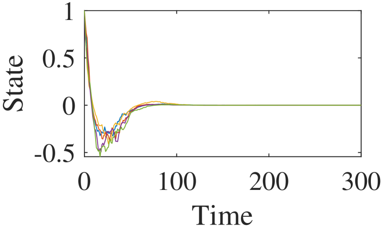
(a) First component $[{\boldsymbol{x}_{t}}]_{1}$

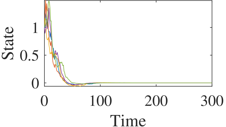
(b) Second component $[{\boldsymbol{x}_{t}}]_{2}$

Figure 5: State transitions for the proposed RRSL control ($\theta=1$).

5.5 Control performance

The next evaluation focuses on the control performance. We compared the RRSL controllers to an existing RN controller ($\theta=0$) that is equivalent to a standard stochastic optimal controller (De Koning, 1982). The expected quadratic cost ${\mathrm{E}_{\boldsymbol{\Lambda}_{0:T}}}[\sum_{t=0}^{T}(\boldsymbol{x}_{t}^{\top}\boldsymbol{Q}\boldsymbol{x}_{t}+\boldsymbol{u}_{t}^{\top}\boldsymbol{R}\boldsymbol{u}_{t})]$ is used as the control performance, where $T=300$ and $\boldsymbol{x}_{0}=[1,1]^{\top}$. We simulate the RRSL control $(\theta>0)$ and the baseline RN control $(\theta=0)$ in $100,000$ trials for each $\theta$.

Figure 6 compares the average values of worse costs over the $100,000$ trials. For each $\rho$, the average value denotes the mean value of the costs ranked in the worst $\rho\%$ in all trials. For example, the average value for $\rho=20$ is calculated as the mean value of the costs ranked in the worst $20,000$ trials. Large values of the sensitivity parameter $\theta$ significantly suppressed the poor results. These results indicate that the proposed RRSL controller successfully handles the risks of the control results.

Figure 6: Average values of worse performance results. For each $\rho$, each average cost denotes the mean value of costs ranked in the worst $\rho\%$ of all the trials.

6 Conclusion

This paper presented a general framework for designing multiple optimal controllers for linear systems with i.i.d. stochastic parameters. They include stochastic optimal, RSL, and the proposed RRSL controllers. The proposed WSR equations are powerful tools for deriving the controllers. The WSR equations are solved via two approaches: using the WSR difference equations and Newton’s method. The stability of the feedback systems was analyzed in terms of MS and WMS.

The proposed general theory has the potential to provide even more types of optimal controllers, by designing weight functions. A further challenge is to find novel optimal controllers using the WSR equations. Additionally, extending the proposed method to other types of stochastic parameters broadens its applicability.

Appendix

Appendix A Supporting results

Let ${\mathrm{E}_{\boldsymbol{\Lambda}}^{\mathrm{q}}}$ denote the expectation with respect to $\boldsymbol{\Lambda}$ that follows another PDF ${f_{\mathrm{q}}(\boldsymbol{\Lambda})}$ instead of ${f_{\mathrm{p}}(\boldsymbol{\Lambda})}$. For any $\boldsymbol{L}$, we define the linear operator ${\mathcal{T}_{\mathrm{q},\boldsymbol{L}}(\boldsymbol{S})}:={\mathrm{E}_{\boldsymbol{\Lambda}}^{\mathrm{q}}}[{{(\boldsymbol{A}-\boldsymbol{B}\boldsymbol{L})}}{}^{\top}\boldsymbol{S}{{(\boldsymbol{A}-\boldsymbol{B}\boldsymbol{L})}}]$, matrix ${\boldsymbol{M}_{\mathrm{q},\boldsymbol{L}}}:={\mathrm{E}_{\boldsymbol{\Lambda}}^{\mathrm{q}}}[$ ${{(\boldsymbol{A}-\boldsymbol{B}\boldsymbol{L})}}{}^{\top}\otimes{{(\boldsymbol{A}-\boldsymbol{B}\boldsymbol{L})}}{}^{\top}]$, and compression operator ${\mathcal{C}(\boldsymbol{D})}:={\mathcal{L}_{n}}\boldsymbol{D}{\mathcal{D}_{n}}$ (Ito and Fujimoto, 2020, Definition 3).

Definition 6 (Stable linear transformations).

Given $\boldsymbol{L}$, the function ${\mathcal{T}_{\mathrm{q},\boldsymbol{L}}}$ is said to be stable if the spectral radius of ${\mathcal{C}({\boldsymbol{M}_{\mathrm{q},\boldsymbol{L}}})}$, that is, the maximum absolute value of the eigenvalues, is less than 1.

Lemma 2 (Equivalence of stable properties).

The following conditions are equivalent.

1. The operator ${\mathcal{T}_{\mathrm{q},\boldsymbol{L}}}$ is stable.

2. For some $\boldsymbol{S}_{2}\succ 0\in{\mathbb{R}_{\mathrm{sym}}^{n}}$, $\lim_{s\rightarrow\infty}{\mathcal{T}_{\mathrm{q},\boldsymbol{L}}^{s}(\boldsymbol{S}_{2})}$ $=0$.

3. For any $\boldsymbol{S}\succeq 0\in{\mathbb{R}_{\mathrm{sym}}^{n}}$, $\lim_{s\rightarrow\infty}{\mathcal{T}_{\mathrm{q},\boldsymbol{L}}^{s}(\boldsymbol{S})}=0$.

Proof.

Firstly, we prove (i) $\Rightarrow$ (ii) similarly to (Ito and Fujimoto, 2020, Appendix A). We have $\mathrm{vech}({\mathcal{T}_{\mathrm{q},\boldsymbol{L}}(\boldsymbol{S})})={\mathcal{L}_{n}}\mathrm{vec}({\mathcal{T}_{\mathrm{q},\boldsymbol{L}}(\boldsymbol{S})})={\mathcal{L}_{n}}{\boldsymbol{M}_{\mathrm{q},\boldsymbol{L}}}\mathrm{vec}(\boldsymbol{S})={\mathcal{C}(\boldsymbol{M}_{\mathrm{q},\boldsymbol{L}})}\mathrm{vech}(\boldsymbol{S})$ and thus $\mathrm{vech}({\mathcal{T}_{\mathrm{q},\boldsymbol{L}}^{s}(\boldsymbol{S})})={\mathcal{C}(\boldsymbol{M}_{\mathrm{q},\boldsymbol{L}})}$ $\mathrm{vech}({\mathcal{T}_{\mathrm{q},\boldsymbol{L}}^{s-1}(\boldsymbol{S})})=\dots={\mathcal{C}(\boldsymbol{M}_{\mathrm{q},\boldsymbol{L}})}^{s}{\mathrm{vech}(\boldsymbol{S})}$ for any symmetric $\boldsymbol{S}$. Thus, (i) implies (ii) because $\mathrm{vech}(\mathcal{T}_{\mathrm{q},\boldsymbol{L}}^{s}(\boldsymbol{S}_{2}))={\mathcal{C}(\boldsymbol{M}_{\mathrm{q},\boldsymbol{L}})}^{s}\mathrm{vech}(\boldsymbol{S}_{2})\to 0$ holds as $s\to\infty$.

Next, we prove (ii) $\Rightarrow$ (iii) in a manner similar to (De Koning, 1982, the proof of Lemma 2.1). For any $\boldsymbol{S}\succeq 0$ and $\boldsymbol{S}_{2}\succ 0$, there exists $\kappa\in\mathbb{R}$ such that $0\preceq\boldsymbol{S}\preceq\kappa\boldsymbol{S}_{2}$. Because of the monotonicity of ${\mathcal{T}_{\mathrm{q},\boldsymbol{L}}^{s}}$, we obtain $0={\mathcal{T}_{\mathrm{q},\boldsymbol{L}}^{s}(0)}\preceq{\mathcal{T}_{\mathrm{q},\boldsymbol{L}}^{s}(\boldsymbol{S})}\preceq{\mathcal{T}_{\mathrm{q},\boldsymbol{L}}^{s}(\kappa\boldsymbol{S}_{2})}=\kappa{\mathcal{T}_{\mathrm{q},\boldsymbol{L}}^{s}(\boldsymbol{S}_{2})}\to 0$ as $s\to\infty$. This implies that (ii) $\Rightarrow$ (iii).

Next, we prove (iii) $\Rightarrow$ (i) similar to (Ito and Fujimoto, 2020, Appendix C). Define $\boldsymbol{S}_{i,j}:=({\boldsymbol{e}_{i}}+{\boldsymbol{e}_{j}})({\boldsymbol{e}_{i}}+{\boldsymbol{e}_{j}})^{\top}\succeq 0$ for $i\in\{1,\dots,n\}$ and $j\in\{i,\dots,n\}$, where ${\boldsymbol{e}_{i}}\in\mathbb{R}^{n}$ satisfies ${[{\boldsymbol{e}_{i}}]_{i}}=1$ and the other components are zero. From (iii), for any $\mathrm{vech}(\boldsymbol{S}_{i,j})\in\mathbb{R}^{n(n+1)/2}$, we have ${\mathcal{C}(\boldsymbol{M}_{\mathrm{q},\boldsymbol{L}})}^{s}\mathrm{vech}(\boldsymbol{S}_{i,j})=\mathrm{vech}({\mathcal{T}_{\mathrm{q},\boldsymbol{L}}^{s}(\boldsymbol{S}_{i,j})})\to 0$ as $s\to\infty$. Because the basis on $\mathbb{R}^{n(n+1)/2}$ consists of linear combinations of $\mathrm{vech}(\boldsymbol{S}_{i,j})$, for any $\boldsymbol{v}\in\mathbb{R}^{n(n+1)/2}$, we have ${\mathcal{C}(\boldsymbol{M}_{\mathrm{q},\boldsymbol{L}})}^{s}\boldsymbol{v}\to 0$, which leads to ${\mathcal{C}(\boldsymbol{M}_{\mathrm{q},\boldsymbol{L}})}^{s}\to 0$. Because the spectral radius of ${\mathcal{C}(\boldsymbol{M}_{\mathrm{q},\boldsymbol{L}})}$ is less than 1, (i) holds. This completes the proof. ∎

We review an existing stochastic optimal control problem (De Koning, 1982).

Definition 7 (Stochastic optimal control problem).

Given a PDF $f_{\mathrm{q}}(\boldsymbol{\Lambda})$ of $\boldsymbol{\Lambda}$, consider the system (1) with $\boldsymbol{\Lambda}_{t}$ that obeys ${f_{\mathrm{q}}(\boldsymbol{\Lambda})}$ instead of ${f_{\mathrm{p}}(\boldsymbol{\Lambda})}$. Consider the cost function ${J_{\infty}(\boldsymbol{u}_{0:\infty},\boldsymbol{x}_{0};\theta)}{|_{w=1}^{\mathrm{q}}}$, where ${|_{w=1}^{\mathrm{q}}}$ denotes the following three conditions: 1) $w_{\mathrm{d}}={w(\boldsymbol{\Lambda};\theta)}=1$ holds for all $\boldsymbol{\Lambda}$, 2) the expectations are taken with a biased PDF ${f_{\mathrm{q}}(\boldsymbol{\Lambda})}$, that is, ${\mathrm{E}_{\boldsymbol{\Lambda}}}$ is replaced with ${\mathrm{E}_{\boldsymbol{\Lambda}}^{\mathrm{q}}}$, and 3) the controller is not restricted as a time-invariant feedback controller, that is, the argument ${\boldsymbol{u}}(\bullet)$ can be replaced with $\boldsymbol{u}_{0:\infty}$. With these settings, Problem 1 is said to be the standard stochastic optimal control problem (SSOCP) with $f_{\mathrm{q}}(\boldsymbol{\Lambda})$.

Lemma 3 ((De Koning, 1982)).

If the SSOCP with $f_{\mathrm{q}}(\boldsymbol{\Lambda})$ is considered, the following results hold.

1. (Lemma 3.1) For any $\boldsymbol{S}\in{\mathbb{R}_{\mathrm{sym}}^{n}}$ and any $\boldsymbol{L}$, the feedback system (3) with ${\boldsymbol{u}}(\boldsymbol{x}_{t})=-\boldsymbol{L}\boldsymbol{x}_{t}$ satisfies ${\mathrm{E}_{\boldsymbol{\Lambda}_{0:t-1}}^{\mathrm{q}}}[\boldsymbol{x}_{t}^{\top}{\boldsymbol{S}}\boldsymbol{x}_{t}]=\boldsymbol{x}_{0}^{\top}{\mathcal{T}_{\mathrm{q},\boldsymbol{L}}^{t}(\boldsymbol{S})}\boldsymbol{x}_{0}$.

2. (Theorem 3.2) Given $\boldsymbol{L}$, the feedback system (3) with ${\boldsymbol{u}}(\boldsymbol{x}_{t})=-\boldsymbol{L}\boldsymbol{x}_{t}$ is MS stable if and only if ${\mathcal{T}_{\mathrm{q},\boldsymbol{L}}}$ is stable.

3. (Theorem 3.3) The system (3) is MS stabilizable if and only if there exists $\boldsymbol{L}$ such that ${\mathcal{T}_{\mathrm{q},\boldsymbol{L}}}$ is stable.

4. (Lemma 2.2) Given $\boldsymbol{S}_{2}\succ 0\in{\mathbb{R}_{\mathrm{sym}}^{n}}$, there exists a solution $\boldsymbol{S}_{1}\succ 0\in{\mathbb{R}_{\mathrm{sym}}^{n}}$ to $\boldsymbol{S}_{1}={\mathcal{T}_{\mathrm{q},\boldsymbol{L}}(\boldsymbol{S}_{1})}+\boldsymbol{S}_{2}$ if and only if ${\mathcal{T}_{\mathrm{q},\boldsymbol{L}}}$ is stable.

5. (Theorems 4.3 and 5.1) Suppose that the feedback system (3) is MS stabilizable. Then, there exists ${\boldsymbol{\Pi}_{\ast\ast}}=\lim_{s\to\infty}{\boldsymbol{F}_{\mathrm{q}}^{s}(0)}$, and it is the minimal nonnegative definite solution to $\boldsymbol{\Pi}={\boldsymbol{F}_{\mathrm{q}}(\boldsymbol{\Pi})}$:

   $${\boldsymbol{F}_{\mathrm{q}}(\boldsymbol{\Pi})} :={\mathrm{E}_{\boldsymbol{\Lambda}}^{\mathrm{q}}}[\boldsymbol{A}^{\top}\boldsymbol{\Pi}\boldsymbol{A}]+\boldsymbol{Q}-{\mathrm{E}_{\boldsymbol{\Lambda}}^{\mathrm{q}}}[\boldsymbol{A}^{\top}\boldsymbol{\Pi}\boldsymbol{B}]{\boldsymbol{G}_{\mathrm{q}}(\boldsymbol{\Pi})}$$

   $$={\mathcal{T}_{\mathrm{q},{\boldsymbol{G}_{\mathrm{q}}(\boldsymbol{\Pi})}}(\boldsymbol{\Pi})}+{\boldsymbol{G}_{\mathrm{q}}(\boldsymbol{\Pi})}^{\top}\boldsymbol{R}{\boldsymbol{G}_{\mathrm{q}}(\boldsymbol{\Pi})}+\boldsymbol{Q},$$ (31)

   $${\boldsymbol{G}_{\mathrm{q}}(\boldsymbol{\Pi})} :={\mathrm{E}_{\boldsymbol{\Lambda}}^{\mathrm{q}}}[\boldsymbol{B}^{\top}\boldsymbol{\Pi}\boldsymbol{B}+\boldsymbol{R}]^{-1}{\mathrm{E}_{\boldsymbol{\Lambda}}^{\mathrm{q}}}[\boldsymbol{B}^{\top}\boldsymbol{\Pi}\boldsymbol{A}].$$ (32)

6. (Theorem 5.2) Suppose that there exists ${\boldsymbol{\Pi}_{\ast\ast}}=\lim_{s\to\infty}{\boldsymbol{F}_{\mathrm{q}}^{s}(0)}$. Then, we have $\boldsymbol{x}_{0}^{\top}{\boldsymbol{\Pi}_{\ast\ast}}\boldsymbol{x}_{0}=\min_{\boldsymbol{u}_{0:\infty}}$ ${J_{\infty}({\boldsymbol{u}_{0:\infty}},\boldsymbol{x}_{0};\theta)}{|_{w=1}^{\mathrm{q}}}$, and the optimal input is $\boldsymbol{u}_{t}={\boldsymbol{L}_{\ast\ast}}\boldsymbol{x}_{t}$ with ${\boldsymbol{L}_{\ast\ast}}:={\boldsymbol{G}_{\mathrm{q}}({\boldsymbol{\Pi}_{\ast\ast}})}$.

7. (Theorem 5.3) Suppose that there exists ${\boldsymbol{\Pi}_{\ast\ast}}=\lim_{s\to\infty}{\boldsymbol{F}_{\mathrm{q}}^{s}(0)}$. Then, ${\boldsymbol{\Pi}_{\ast\ast}}$ is positive definite and the unique solution to $\boldsymbol{\Pi}={\boldsymbol{F}_{\mathrm{q}}(\boldsymbol{\Pi})}$. In addition, ${\mathcal{T}_{\mathrm{q},{\boldsymbol{L}_{\ast\ast}}}}$ is stable.

Remark 8.

The definitions of the stable and stabilizable properties of ${\mathcal{T}_{\mathrm{q},\boldsymbol{L}}}$ in this study are different from those in (De Koning, 1982). Regardless of this difference, Lemma 3 is proven in the same manner as the original version, using Lemma 2. For example, similarly to (De Koning, 1982, Lemma 2.2 (a)), if ${\mathcal{T}_{\mathrm{q},\boldsymbol{L}}}$ is stable, there exists $\boldsymbol{S}_{1}=\sum_{s=0}^{\infty}{\mathcal{T}_{\mathrm{q},\boldsymbol{L}}^{s}(\boldsymbol{S}_{2})}$ because $\mathrm{vech}(\boldsymbol{S}_{1})=\sum_{s=0}^{\infty}\mathrm{vech}(\mathcal{T}_{\mathrm{q},\boldsymbol{L}}^{s}(\boldsymbol{S}_{2}))=\sum_{s=0}^{\infty}{\mathcal{C}(\boldsymbol{M}_{\mathrm{q},\boldsymbol{L}})}^{s}\mathrm{vech}(\boldsymbol{S}_{2})$ and thus $(\boldsymbol{I}-{\mathcal{C}(\boldsymbol{M}_{\mathrm{q},\boldsymbol{L}})})\mathrm{vech}(\boldsymbol{S}_{1})={\mathrm{vech}(\boldsymbol{S}_{2})}$ hold with the nonsingular $(\boldsymbol{I}-{\mathcal{C}(\boldsymbol{M}_{\mathrm{q},\boldsymbol{L}})})$. In addition, $(\boldsymbol{I}-{\mathcal{C}(\boldsymbol{M}_{\mathrm{q},\boldsymbol{L}})})\mathrm{vech}(\boldsymbol{S}_{1})={\mathrm{vech}(\boldsymbol{S}_{2})}$ is equivalent to $\boldsymbol{S}_{1}={\mathcal{T}_{\mathrm{q},\boldsymbol{L}}(\boldsymbol{S}_{1})}+\boldsymbol{S}_{2}$. Furthermore, our definitions are advantageous because the spectral radius of ${\mathcal{C}(\boldsymbol{M}_{\mathrm{q},\boldsymbol{L}})}$ is easy to evaluate. Lemma 3 (ii) and (iii) are equivalent to Proposition 1 if ${f_{\mathrm{q}}(\boldsymbol{\Lambda})}={f_{\mathrm{p}}(\boldsymbol{\Lambda})}$ holds.

Appendix B Proof of Theorem 1

Firstly, we show that some statements in Lemma 3 in Appendix A can be utilized because there exists a solution $({\boldsymbol{\Pi}_{\ast}},{\boldsymbol{L}_{\ast}})$ to the WSR equations (11) and (12). Let us consider the system (1) with $\boldsymbol{\Lambda}_{t}$ that obeys the biased PDF ${f_{\mathrm{q}}(\boldsymbol{\Lambda})}=w_{\mathrm{d}}(\boldsymbol{\Lambda};\theta,\widetilde{\boldsymbol{u}}(\bullet;{\boldsymbol{L}_{\ast}}),\widetilde{J}(\bullet;{\boldsymbol{\Pi}_{\ast}}))f_{\mathrm{p}}(\boldsymbol{\Lambda})$ called the biased system. Because of Assumption 1, ${f_{\mathrm{q}}(\boldsymbol{\Lambda})}$ is a continuous PDF satisfying $\int_{\mathbb{S}_{\boldsymbol{\Lambda}}}{f_{\mathrm{q}}(\boldsymbol{\Lambda})}\mathrm{d}\boldsymbol{\Lambda}=1$ and ${f_{\mathrm{q}}(\boldsymbol{\Lambda})}\geq 0$. Then, the WSR equations with $({\boldsymbol{\Pi}_{\ast}},{\boldsymbol{L}_{\ast}})$ reduce to ${\boldsymbol{\Pi}_{\ast}}={\boldsymbol{F}_{\mathrm{q}}({\boldsymbol{\Pi}_{\ast}})}$ and ${\boldsymbol{L}_{\ast}}:={\boldsymbol{G}_{\mathrm{q}}({\boldsymbol{\Pi}_{\ast}})}$ with (31) and (32) because the weighted expectation ${\mathcal{E}_{\boldsymbol{\Lambda}}^{(\theta,{\boldsymbol{L}_{\ast}},{\boldsymbol{\Pi}_{\ast}})}}$ is replaced with the expectation ${\mathrm{E}_{\boldsymbol{\Lambda}}^{\mathrm{q}}}$. Because ${\boldsymbol{\Pi}_{\ast}}$ is a positive definite solution to (31), the biased system is MS stabilizable by Lemma 3 (iv) and (iii). This enables to utilize Lemma 3 (v), (vi), and (vii).

Using the solution $({\boldsymbol{\Pi}_{\ast}},{\boldsymbol{L}_{\ast}})$, we set the weight as follows:

$$\forall\boldsymbol{\Lambda},\;{w(\boldsymbol{\Lambda};\theta)} =w_{\mathrm{d}}(\boldsymbol{\Lambda};\theta,\widetilde{\boldsymbol{u}}(\bullet;{\boldsymbol{L}_{\ast}}),\widetilde{J}(\bullet;{\boldsymbol{\Pi}_{\ast}})).$$ (33)

The cost function ${J_{\infty}({\boldsymbol{u}},\boldsymbol{x}_{0};\theta)}$ with (33) is equivalent to ${J_{\infty}({\boldsymbol{u}},\boldsymbol{x}_{0};\theta)}{|_{w=1}^{\mathrm{q}}}$ because ${\mathrm{E}_{\boldsymbol{\Lambda}_{0:t}}}[\prod_{s=0}^{t}{w(\boldsymbol{\Lambda}_{s};\theta)}(\dots)]={\mathrm{E}_{\boldsymbol{\Lambda}_{0:t}}^{\mathrm{q}}}[(\dots)]$ holds. Solving (5) and (6) reduces to solving the SSOCP with ${f_{\mathrm{q}}(\boldsymbol{\Lambda})}$ in Definition 7. From Lemma 3 (v) and (vi), the optimal controller and minimum cost are $\widetilde{\boldsymbol{u}}(\boldsymbol{x};{\boldsymbol{L}_{\ast\ast}})$ and $\widetilde{J}(\boldsymbol{x};{\boldsymbol{\Pi}_{\ast\ast}})$, respectively. Lemma 3 (vii) implies the uniqueness of the solution, that is, ${\boldsymbol{\Pi}_{\ast\ast}}={\boldsymbol{\Pi}_{\ast}}$ and ${\boldsymbol{L}_{\ast\ast}}={\boldsymbol{L}_{\ast}}$ hold. Therefore, $\boldsymbol{u}_{\ast}(\boldsymbol{x})=-{\boldsymbol{L}_{\ast}}\boldsymbol{x}=\widetilde{\boldsymbol{u}}(\boldsymbol{x};{\boldsymbol{L}_{\ast}})$ and $J_{\ast}(\boldsymbol{x})=\boldsymbol{x}^{\top}{\boldsymbol{\Pi}_{\ast}}\boldsymbol{x}=\widetilde{J}(\boldsymbol{x};{\boldsymbol{\Pi}_{\ast}})$ are solutions to (5) and (6), respectively, and (33) is equivalent to (7). This completes the proof.

Appendix C Proof of Theorem 2

In this proof, a solution to the WSR equations (11) and (12) for each $\theta$ is explicitly denoted by $({\boldsymbol{\Pi}_{\ast}}(\theta)\succ 0,{\boldsymbol{L}_{\ast}}(\theta))$, and its vectorization is denoted by ${\boldsymbol{z}_{\ast}(\theta)}$. Note that ${\boldsymbol{h}(\boldsymbol{z},0)}=0$ reduces to $\boldsymbol{\Pi}={\boldsymbol{F}_{\mathrm{q}}(\boldsymbol{\Pi})}$ and $\boldsymbol{L}:={\boldsymbol{G}_{\mathrm{q}}(\boldsymbol{\Pi})}$ with (31), (32), and ${f_{\mathrm{q}}(\boldsymbol{\Lambda})}={f_{\mathrm{p}}(\boldsymbol{\Lambda})}$. Because of Assumption 2 (i) and (ii) and Lemma 3 (v) and (vii), there exist unique ${{\boldsymbol{\Pi}_{\ast}}(0)}\succ 0$ and ${{\boldsymbol{L}_{\ast}}(0)}={\boldsymbol{G}_{\mathrm{q}}({\boldsymbol{\Pi}_{\ast}}(0))}$, that is, ${\boldsymbol{z}_{\ast}(0)}\in\mathbb{S}_{\boldsymbol{z}}$. We now prove the following statements:

1. There exist open sets $\mathbb{B}_{\theta}$ and $\mathbb{B}_{\boldsymbol{z}}$ such that $(0,{\boldsymbol{z}_{\ast}(0)})\in\mathbb{B}_{\theta}\times\mathbb{B}_{\boldsymbol{z}}\subset\mathbb{R}\times\mathbb{R}^{(n(n+1)/2)+mn}$ holds and there exists a unique $C^{1}$ continuous function ${\boldsymbol{z}_{\ast}(\bullet)}:\mathbb{B}_{\theta}\to\mathbb{B}_{\boldsymbol{z}}$ satisfying ${\boldsymbol{h}(\boldsymbol{z}_{\ast}(\theta),\theta)}=0$.

2. There exist $\mathbb{B}_{\theta}$ and $\mathbb{B}_{\boldsymbol{z}}$ such that $\mathbb{B}_{\theta}$ is connected, $\mathbb{B}_{\boldsymbol{z}}\subset\mathbb{S}_{\boldsymbol{z}}$ holds, and all the conditions in (S1) hold.

Firstly, ${\boldsymbol{h}(\boldsymbol{z},\theta)}$ is $C^{2}$ continuous on a neighborhood of $({\boldsymbol{z}_{\ast}(0)},0)$ because of Assumption 2. Next, we prove that $\partial_{\boldsymbol{z}^{\top}}{\boldsymbol{h}(\boldsymbol{z}_{\ast}(0),0)}$ is nonsingular. Note that $\mathrm{vec}(\boldsymbol{C}_{1}\boldsymbol{C}_{2}\boldsymbol{C}_{3})=(\boldsymbol{C}_{3}^{\top}\otimes\boldsymbol{C}_{1})\mathrm{vec}(\boldsymbol{C}_{2})$ for given $\boldsymbol{C}_{1}$, $\boldsymbol{C}_{2}$, and $\boldsymbol{C}_{3}$ (Gentle, 2017, Section 3.2.10.2). Using a relationship similar to $\mathrm{vech}({\mathcal{T}_{\mathrm{q},\boldsymbol{L}}(\boldsymbol{S})})={\mathcal{C}(\boldsymbol{M}_{\mathrm{q},\boldsymbol{L}})}\mathrm{vech}(\boldsymbol{S})$ in Appendix A, we derive the several representations of ${\boldsymbol{f}(\boldsymbol{z},\theta)}$ and ${\boldsymbol{g}(\boldsymbol{z},\theta)}$:

$${\boldsymbol{f}(\boldsymbol{z},\theta)} =\mathcal{C}({\mathcal{E}_{\boldsymbol{\Lambda}}^{(\theta,\boldsymbol{L},\boldsymbol{\Pi})}}[{{(\boldsymbol{A}-\boldsymbol{B}\boldsymbol{L})}}^{\top}\otimes{{(\boldsymbol{A}-\boldsymbol{B}\boldsymbol{L})}}^{\top}]-{\boldsymbol{I}_{n^{2}}})$$

$$\quad\times\mathrm{vech}(\boldsymbol{\Pi})+\mathrm{vech}(\boldsymbol{L}^{\top}\boldsymbol{R}\boldsymbol{L}+\boldsymbol{Q})$$

$$=\mathrm{vech}\big{(}{\mathcal{E}_{\boldsymbol{\Lambda}}^{(\theta,\boldsymbol{L},\boldsymbol{\Pi})}}[\boldsymbol{A}^{\top}\boldsymbol{\Pi}\boldsymbol{A}]-\boldsymbol{L}^{\top}{\mathcal{E}_{\boldsymbol{\Lambda}}^{(\theta,\boldsymbol{L},\boldsymbol{\Pi})}}[\boldsymbol{B}^{\top}\boldsymbol{\Pi}\boldsymbol{A}]$$

$$\quad-{\mathcal{E}_{\boldsymbol{\Lambda}}^{(\theta,\boldsymbol{L},\boldsymbol{\Pi})}}[\boldsymbol{A}^{\top}\boldsymbol{\Pi}\boldsymbol{B}]\boldsymbol{L}$$

$$\quad+\boldsymbol{L}^{\top}{\mathcal{E}_{\boldsymbol{\Lambda}}^{(\theta,\boldsymbol{L},\boldsymbol{\Pi})}}[\boldsymbol{B}^{\top}\boldsymbol{\Pi}\boldsymbol{B}+\boldsymbol{R}]\boldsymbol{L}+\boldsymbol{Q}-\boldsymbol{\Pi}\big{)},$$ (34)

$${\boldsymbol{g}(\boldsymbol{z},\theta)} =({\boldsymbol{I}_{n}}\otimes{\mathcal{E}_{\boldsymbol{\Lambda}}^{(\theta,\boldsymbol{L},\boldsymbol{\Pi})}}[\boldsymbol{B}^{\top}\boldsymbol{\Pi}\boldsymbol{B}+\boldsymbol{R}])\mathrm{vec}(\boldsymbol{L})$$

$$\quad-\mathrm{vec}({\mathcal{E}_{\boldsymbol{\Lambda}}^{(\theta,\boldsymbol{L},\boldsymbol{\Pi})}}[\boldsymbol{B}^{\top}\boldsymbol{\Pi}\boldsymbol{A}]).$$ (35)

Assumption 1 with $\theta=0$ implies that for every $(\boldsymbol{\Lambda},\widetilde{\boldsymbol{u}}(\bullet;\boldsymbol{L}),\widetilde{J}(\bullet;\boldsymbol{\Pi}))$, we have $w_{\mathrm{d}}(\boldsymbol{\Lambda};\theta,\widetilde{\boldsymbol{u}}(\bullet;\boldsymbol{L}),\widetilde{J}(\bullet;\boldsymbol{\Pi}))=1$ and thus $\partial w_{\mathrm{d}}(\boldsymbol{\Lambda};\theta,\widetilde{\boldsymbol{u}}(\bullet;\boldsymbol{L}),\widetilde{J}(\bullet;\boldsymbol{\Pi}))/\partial\boldsymbol{z}=0$. The following partial derivatives are obtained from (34) and (35):

$$\frac{\partial}{\partial\mathrm{vech}(\boldsymbol{\Pi})^{\top}}{\boldsymbol{f}(\boldsymbol{z}_{\ast}(0),0)}$$

$$=\mathcal{C}({\mathrm{E}_{\boldsymbol{\Lambda}}}[{{(\boldsymbol{A}-\boldsymbol{B}{{\boldsymbol{L}_{\ast}}(0)})}}^{\top}\otimes{{(\boldsymbol{A}-\boldsymbol{B}{{\boldsymbol{L}_{\ast}}(0)})}}^{\top}])$$

$$\quad-{\boldsymbol{I}_{n(n+1)/2}},$$ (36)

$$\frac{\partial}{\partial\mathrm{vec}(\boldsymbol{L})^{\top}}{\boldsymbol{g}(\boldsymbol{z}_{\ast}(0),0)}={\boldsymbol{I}_{n}}\otimes{\mathrm{E}_{\boldsymbol{\Lambda}}}[\boldsymbol{B}^{\top}{{\boldsymbol{\Pi}_{\ast}}(0)}\boldsymbol{B}+\boldsymbol{R}].$$ (37)

Note that $\boldsymbol{S}\mapsto{\mathrm{E}_{\boldsymbol{\Lambda}}}[{{(\boldsymbol{A}-\boldsymbol{B}{{\boldsymbol{L}_{\ast}}(0)})}}^{\top}\boldsymbol{S}{{(\boldsymbol{A}-\boldsymbol{B}{{\boldsymbol{L}_{\ast}}(0)})}}]$ is stable by Lemma 3 (vii). Because of Definition 6, the spectral radius of $\mathcal{C}({\mathrm{E}_{\boldsymbol{\Lambda}}}[{{(\boldsymbol{A}-\boldsymbol{B}{{\boldsymbol{L}_{\ast}}(0)})}}^{\top}\otimes{{(\boldsymbol{A}-\boldsymbol{B}{{\boldsymbol{L}_{\ast}}(0)})}}^{\top}])$, that is, maximum absolute value of the eigenvalues, is less than 1 and thus (36) is nonsingular. Because ${\mathrm{E}_{\boldsymbol{\Lambda}}}[\boldsymbol{B}^{\top}{{\boldsymbol{\Pi}_{\ast}}(0)}\boldsymbol{B}+\boldsymbol{R}]\succ 0$, the block diagonal matrix $\partial_{\mathrm{vec}(\boldsymbol{L})^{\top}}{\boldsymbol{g}(\boldsymbol{z}_{\ast}(0),0)}$ in (37) is nonsingular. The following partial derivative is calculated from (34):

$$\frac{\partial}{\partial{[{\boldsymbol{L}}]_{i,j}}}{\boldsymbol{f}(\boldsymbol{z},0)}$$

$$=\mathrm{vech}\Big{(}\frac{\partial\boldsymbol{L}^{\top}}{\partial{[{\boldsymbol{L}}]_{i,j}}}\Big{(}{\mathrm{E}_{\boldsymbol{\Lambda}}}[\boldsymbol{B}^{\top}\boldsymbol{\Pi}\boldsymbol{B}+\boldsymbol{R}]\boldsymbol{L}-{\mathrm{E}_{\boldsymbol{\Lambda}}}[\boldsymbol{B}^{\top}\boldsymbol{\Pi}\boldsymbol{A}]\Big{)}$$

$$\quad+\Big{(}\boldsymbol{L}^{\top}{\mathrm{E}_{\boldsymbol{\Lambda}}}[\boldsymbol{B}^{\top}\boldsymbol{\Pi}\boldsymbol{B}+\boldsymbol{R}]-{\mathrm{E}_{\boldsymbol{\Lambda}}}[\boldsymbol{A}^{\top}\boldsymbol{\Pi}\boldsymbol{B}]\Big{)}\frac{\partial\boldsymbol{L}}{\partial{[{\boldsymbol{L}}]_{i,j}}}\Big{)}.$$ (38)

We have $\partial_{\mathrm{vec}(\boldsymbol{L})^{\top}}{\boldsymbol{f}(\boldsymbol{z}_{\ast}(0),0)}=0$ by substituting ${\boldsymbol{z}_{\ast}(0)}$ with ${{\boldsymbol{L}_{\ast}}(0)}={\mathrm{E}_{\boldsymbol{\Lambda}}}[\boldsymbol{B}^{\top}{\boldsymbol{\Pi}_{\ast}}(0)\boldsymbol{B}+\boldsymbol{R}]^{-1}{\mathrm{E}_{\boldsymbol{\Lambda}}}[\boldsymbol{B}^{\top}{\boldsymbol{\Pi}_{\ast}}(0)\boldsymbol{A}]$ into (38). Thus, $\partial_{\boldsymbol{z}^{\top}}{\boldsymbol{h}(\boldsymbol{z}_{\ast}(0),0)}$ is the block triangular matrix that is nonsingular because we have nonzero determinants $\det|\partial_{\mathrm{vec}(\boldsymbol{\Pi})^{\top}}{\boldsymbol{f}(\boldsymbol{z}_{\ast}(0),0)}|\neq 0$ and $\det|\partial_{\mathrm{vec}(\boldsymbol{L})^{\top}}{\boldsymbol{g}(\boldsymbol{z}_{\ast}(0),0)}|\neq 0$ (Gentle, 2017, Section 3.1.9.7). Then, (S1) holds according to the implicit function theorem (de Oliveira, 2013, Theorem 5). We obtain (S2) by choosing $\mathbb{B}_{\theta}$ as a small ball of $0$ because $\mathbb{B}_{\theta}$ and $\mathbb{B}_{\boldsymbol{z}}$ contain open balls of $0$ and ${\boldsymbol{z}_{\ast}(0)}$, respectively, and ${\boldsymbol{z}_{\ast}(\bullet)}$ is continuous.

Using (S2), we prove Theorem 2 as follows. Let $\mathbb{S}_{\boldsymbol{z},2}:=\mathbb{S}_{\boldsymbol{z}}\setminus\mathbb{B}_{\boldsymbol{z}}$. Because $\mathbb{S}_{\boldsymbol{z},2}$ is a bounded closed set, $\|{\boldsymbol{h}(\boldsymbol{z},0)}\|$ is continuous on $\mathbb{S}_{\boldsymbol{z},2}$, and the uniqueness of ${\boldsymbol{z}_{\ast}(0)}$ indicates ${\boldsymbol{h}(\boldsymbol{z},0)}\neq 0$ on $\mathbb{S}_{\boldsymbol{z},2}$, there exists $\delta_{h}>0$ that satisfies $\|{\boldsymbol{h}(\boldsymbol{z},0)}\|>\delta_{h}$ for every $\boldsymbol{z}\in\mathbb{S}_{\boldsymbol{z},2}$. For some $\underline{\theta}<0$ and $\overline{\theta}>0$ that satisfy $[\underline{\theta},\overline{\theta}]\subset\mathbb{B}_{\theta}$, $\partial_{\theta}{\boldsymbol{h}(\boldsymbol{z},\theta)}$ is bounded on the bounded closed set $\mathbb{S}_{\boldsymbol{z},2}\times[\underline{\theta},\overline{\theta}]$ because of the continuity. Namely, there exists $\delta_{\partial h}>0$ such that $\|\partial_{\theta}{\boldsymbol{h}(\boldsymbol{z},\theta)}\|\leq\delta_{\partial h}$. Here, we set $\underline{\theta}_{\mathrm{u}}=\max\{-\delta_{h}/\delta_{\partial h},\underline{\theta}\}<0$ and $\overline{\theta}_{\mathrm{u}}=\min\{\delta_{h}/\delta_{\partial h},\overline{\theta}\}>0$. Then, for any $(\boldsymbol{z},\theta)\in\mathbb{S}_{\boldsymbol{z},2}\times[\underline{\theta}_{\mathrm{u}},\overline{\theta}_{\mathrm{u}}]$, we have

$$\|{\boldsymbol{h}(\boldsymbol{z},\theta)}\|\geq\|{\boldsymbol{h}(\boldsymbol{z},0)}\|-\delta_{\partial h}|\theta|>\delta_{h}-\delta_{\partial h}|\theta|\geq 0.$$ (39)

Thus, there exists no solution to ${\boldsymbol{h}(\boldsymbol{z},\theta)}=0$ on $(\mathbb{S}_{\boldsymbol{z}}\setminus\mathbb{B}_{\boldsymbol{z}})\times[\underline{\theta}_{\mathrm{u}},\overline{\theta}_{\mathrm{u}}]$. Meanwhile, there exist a unique solution $({\boldsymbol{z}_{\ast}(\theta)},\theta)$ on $\mathbb{B}_{\boldsymbol{z}}\times[\underline{\theta}_{\mathrm{u}},\overline{\theta}_{\mathrm{u}}]$ because $[\underline{\theta}_{\mathrm{u}},\overline{\theta}_{\mathrm{u}}]\subset\mathbb{B}_{\theta}$ holds. Therefore, there exists a unique ${\boldsymbol{z}_{\ast}(\bullet)}:[\underline{\theta}_{\mathrm{u}},\overline{\theta}_{\mathrm{u}}]\to\mathbb{S}_{\boldsymbol{z}}$ that satisfies ${\boldsymbol{h}(\boldsymbol{z}_{\ast}(\theta),\theta)}=0$ and $C^{1}$ continuous on $(\underline{\theta}_{\mathrm{u}},\overline{\theta}_{\mathrm{u}})$. The positive definiteness ${\boldsymbol{\Pi}_{\ast}}\succ 0$ holds form the definition of $\mathbb{S}_{\boldsymbol{\Pi}}$. This completes the proof.

Appendix D Proof of Theorem 3

We prove the statement by taking the limit $s\rightarrow\infty$ in a manner similar to (De Koning, 1982, Theorem 5.1). Because ${\boldsymbol{H}(\bullet,\bullet;\theta)}:=[{\boldsymbol{F}(\bullet,\bullet;\theta)},{\boldsymbol{G}(\bullet,\bullet;\theta)}{}^{\top}]$ is continuous at $(\widehat{\boldsymbol{\Pi}_{\ast}},\widehat{\boldsymbol{L}_{\ast}})$, using (25) yields $\lim_{s\rightarrow\infty}{\boldsymbol{H}(\boldsymbol{\Pi}_{s},\boldsymbol{L}_{s};\theta)}={\boldsymbol{H}(\widehat{\boldsymbol{\Pi}_{\ast}},\widehat{\boldsymbol{L}_{\ast}};\theta)}$ as follows:

$$\forall \epsilon>0,\quad\exists\delta>0,\quad\exists s^{\prime}>0,$$

$$s>s^{\prime} \Rightarrow\|{[{\boldsymbol{\Pi}_{s}},{\boldsymbol{L}_{s}}{}^{\top}]-[\widehat{\boldsymbol{\Pi}_{\ast}},\widehat{\boldsymbol{L}_{\ast}}{}^{\top}]}\|_{\mathrm{F}}<\delta$$

$$\Rightarrow\|{{\boldsymbol{H}(\boldsymbol{\Pi}_{s},\boldsymbol{L}_{s};\theta)}-{\boldsymbol{H}(\widehat{\boldsymbol{\Pi}_{\ast}},\widehat{\boldsymbol{L}_{\ast}};\theta)}}\|_{\mathrm{F}}<\epsilon,$$ (40)

where $\|{\bullet}\|_{\mathrm{F}}$ is the Frobenius norm. Thus, we obtain $[\widehat{\boldsymbol{\Pi}_{\ast}},\widehat{\boldsymbol{L}_{\ast}}{}^{\top}]=\lim_{s\rightarrow\infty}[{\boldsymbol{\Pi}_{s}},{\boldsymbol{L}_{s}}{}^{\top}]=\lim_{s\rightarrow\infty}[{\boldsymbol{\Pi}_{s+1}},{\boldsymbol{L}_{s+1}}{}^{\top}]$ $={\boldsymbol{H}(\widehat{\boldsymbol{\Pi}_{\ast}},\widehat{\boldsymbol{L}_{\ast}};\theta)}$. Next, (24) is transformed into

$${\boldsymbol{\Pi}_{s+1}} ={\mathcal{E}_{\boldsymbol{\Lambda}}^{(\theta,\boldsymbol{L}_{s},\boldsymbol{\Pi}_{s})}}[(\boldsymbol{A}-\boldsymbol{B}{\boldsymbol{G}(\boldsymbol{\Pi}_{s},\boldsymbol{L}_{s};\theta)})^{\top}$$

$$\quad\times{\boldsymbol{\Pi}_{s}}(\boldsymbol{A}-\boldsymbol{B}{\boldsymbol{G}(\boldsymbol{\Pi}_{s},\boldsymbol{L}_{s};\theta)})]$$

$$\quad+{\boldsymbol{G}(\boldsymbol{\Pi}_{s},\boldsymbol{L}_{s};\theta)}^{\top}\boldsymbol{R}{\boldsymbol{G}(\boldsymbol{\Pi}_{s},\boldsymbol{L}_{s};\theta)}+\boldsymbol{Q}.$$ (41)

Because $w_{\mathrm{d}}(\boldsymbol{\Lambda};\theta,\widetilde{\boldsymbol{u}}(\bullet;\boldsymbol{L}),\widetilde{J}(\bullet;\boldsymbol{\Pi}))\geq 0$ holds, the positive semidefiniteness of ${\boldsymbol{\Pi}_{0}}\succeq 0$ implies ${\boldsymbol{\Pi}_{s}}\succeq\boldsymbol{Q}\succ 0$ for any $s$, which yields $\widehat{\boldsymbol{\Pi}_{\ast}}\succ 0$. This completes the proof.

Appendix E Proof of Theorem 4

In this proof, let $\|\boldsymbol{C}\|$ be the induced norm of a given matrix $\boldsymbol{C}$. Because of Assumption 2 (iii), ${\boldsymbol{h}(\boldsymbol{z},\theta)}$ is $C^{2}$ continuous, and thus $\partial_{\boldsymbol{z}^{\top}}{\boldsymbol{h}(\boldsymbol{z},\theta)}$ is Lipschitz continuous on $\mathbb{S}_{\boldsymbol{z}}\times[\underline{\theta}_{\mathrm{s}},\overline{\theta}_{\mathrm{s}}]$. Let $\gamma_{\partial\boldsymbol{h}{}{}}$ be a Lipschitz constant of $\partial_{\boldsymbol{z}^{\top}}{\boldsymbol{h}(\boldsymbol{z},\theta)}$ on this set. In addition, for some $\underline{\theta}_{\mathrm{u}}\geq\underline{\theta}_{\mathrm{s}}$ and $\overline{\theta}_{\mathrm{u}}\leq\overline{\theta}_{\mathrm{s}}$, for every $\theta\in[\underline{\theta}_{\mathrm{u}},\overline{\theta}_{\mathrm{u}}]$, ${\boldsymbol{z}_{\ast}(\theta)}$ is a unique solution by Theorem 2. Based on the proofs in (Kelley, 1995, Lemma 4.3.1 and Theorem 5.1.1), the q-quadratical convergence holds in Lemma 1 if the standard assumptions and ${\boldsymbol{z}_{0}}={\boldsymbol{z}_{\ast}(0)}\in{{\mathbb{B}}_{\boldsymbol{z}}^{\ast}(\delta_{\ast}(\theta),\theta)}$ hold for a scalar ${\delta_{\ast}(\theta)}$ that satisfies $\gamma_{\partial\boldsymbol{h}{}{}}\|\partial_{\boldsymbol{z}^{\top}}{\boldsymbol{h}(\boldsymbol{z}_{\ast}(\theta),\theta)}^{-1}\|\delta_{\ast}(\theta)<1/2$. We define $\delta_{\ast}(\theta):=\gamma^{\prime}/(2\gamma_{\partial\boldsymbol{h}{}{}}\|\partial_{\boldsymbol{z}^{\top}}{\boldsymbol{h}(\boldsymbol{z}_{\ast}(\theta),\theta)}^{-1}\|)$ with a constant $\gamma^{\prime}\in(0,1)$. Thus, Theorem 4 is derived if the following statements hold.

1. There exist an open set $\mathbb{S}_{\boldsymbol{z}}^{\prime}\subset\mathbb{S}_{\boldsymbol{z}}$ containing ${\boldsymbol{z}_{\ast}(0)}$, $\overline{\theta}_{\mathrm{n}}>0$, and $\underline{\theta}_{\mathrm{n}}<0$ such that for every $\theta\in(\underline{\theta}_{\mathrm{n}},\overline{\theta}_{\mathrm{n}})$, the standard assumptions on $(\mathbb{S}_{\boldsymbol{z}}^{\prime},\theta)$ hold.

2. For any open set $\mathbb{S}_{\boldsymbol{z}}^{\prime}\subset\mathbb{S}_{\boldsymbol{z}}$ containing ${\boldsymbol{z}_{\ast}(0)}$, there exist $\delta>0$, $\underline{\theta}_{\mathrm{n}}<0$, and $\overline{\theta}_{\mathrm{n}}>0$ such that for every $\theta\in(\underline{\theta}_{\mathrm{n}},\overline{\theta}_{\mathrm{n}})$, we have ${{\mathbb{B}}_{\boldsymbol{z}}^{\ast}(\delta,\theta)}\subseteq{{\mathbb{B}}_{\boldsymbol{z}}^{\ast}(\delta_{\ast}(\theta),\theta)}$ and ${\boldsymbol{z}_{0}}={\boldsymbol{z}_{\ast}(0)}\in{{\mathbb{B}}_{\boldsymbol{z}}^{\ast}(\delta,\theta)}\subset\mathbb{S}_{\boldsymbol{z}}^{\prime}$.

We prove that the standard assumption (i) holds for deriving (S3). According to Theorem 2, there exists a unique solution ${\boldsymbol{z}_{\ast}(\theta)}\in\mathbb{S}_{\boldsymbol{z}}$ that is $C^{1}$ continuous in $\theta$ on $(\underline{\theta}_{\mathrm{u}},\overline{\theta}_{\mathrm{u}})$. Let $\mathbb{S}_{\boldsymbol{z}}^{\prime}\subset\mathbb{S}_{\boldsymbol{z}}$ be any open ball with the center ${\boldsymbol{z}_{\ast}(0)}$. There exist $\underline{\theta}_{\mathrm{n}}\in[\underline{\theta}_{\mathrm{u}},0)$ and $\overline{\theta}_{\mathrm{n}}\in(0,\overline{\theta}_{\mathrm{u}}]$ such that ${\boldsymbol{z}_{\ast}(\theta)}\in\mathbb{S}_{\boldsymbol{z}}^{\prime}$ holds for any $\theta\in(\underline{\theta}_{\mathrm{n}},\overline{\theta}_{\mathrm{n}})$ because of the continuity. This indicates the standard assumption (i) for any open ball $\mathbb{S}_{\boldsymbol{z}}^{\prime}$ and $\theta\in(\underline{\theta}_{\mathrm{n}},\overline{\theta}_{\mathrm{n}})\subseteq(\underline{\theta}_{\mathrm{u}},\overline{\theta}_{\mathrm{u}})$.

Next, we prove that the standard assumption (ii) holds. Because $\partial_{\boldsymbol{z}^{\top}}{\boldsymbol{h}(\boldsymbol{z},\theta)}$ is Lipschitz continuous on $\mathbb{S}_{\boldsymbol{z}}\times[\underline{\theta}_{\mathrm{s}},\overline{\theta}_{\mathrm{s}}]$ according to Assumption 2, the standard assumption (ii) holds for any open set $\mathbb{S}_{\boldsymbol{z}}^{\prime}\subset\mathbb{S}_{\boldsymbol{z}}$ containing ${\boldsymbol{z}_{\ast}(0)}$ and any $\theta\in[\underline{\theta}_{\mathrm{s}},\overline{\theta}_{\mathrm{s}}]$.

We prove that the standard assumption (iii) holds. According to the standard assumption (ii), let ${d(\boldsymbol{z},\theta)}:=[\boldsymbol{z}^{\top},\theta]-[{\boldsymbol{z}_{\ast}(0)}^{\top},0]$, and we have $\|\partial_{\boldsymbol{z}^{\top}}{\boldsymbol{h}(\boldsymbol{z},\theta)}-\partial_{\boldsymbol{z}^{\top}}{\boldsymbol{h}(\boldsymbol{z}_{\ast}(0),0)}\|\leq\gamma_{\partial\boldsymbol{h}{}{}}\|{d(\boldsymbol{z},\theta)}\|$, where $\partial_{\boldsymbol{z}^{\top}}{\boldsymbol{h}(\boldsymbol{z}_{\ast}(0),0)}$ is nonsingular because of the proof of Theorem 2. We obtain the following result based on (Kelley, 1995, the proof of Lemma 4.3.1):

$$\|{\boldsymbol{I}_{n(m+(n+1)/2)}}-\partial_{\boldsymbol{z}^{\top}}{\boldsymbol{h}(\boldsymbol{z}_{\ast}(0),0)}^{-1}\partial_{\boldsymbol{z}^{\top}}{\boldsymbol{h}(\boldsymbol{z},\theta)}\|$$

$$=\|\partial_{\boldsymbol{z}^{\top}}{\boldsymbol{h}(\boldsymbol{z}_{\ast}(0),0)}^{-1}(\partial_{\boldsymbol{z}^{\top}}{\boldsymbol{h}(\boldsymbol{z}_{\ast}(0),0)}-\partial_{\boldsymbol{z}^{\top}}{\boldsymbol{h}(\boldsymbol{z},\theta)})\|$$

$$\leq\gamma_{\partial\boldsymbol{h}{}{}}\|\partial_{\boldsymbol{z}^{\top}}{\boldsymbol{h}(\boldsymbol{z}_{\ast}(0),0)}^{-1}\|\|{d(\boldsymbol{z},\theta)}\|.$$ (42)

If the right hand side of this inequality is less than 1, the Banach Lemma (Kelley, 1995, Theorem 1.2.1) implies that $\partial_{\boldsymbol{z}^{\top}}{\boldsymbol{h}(\boldsymbol{z},\theta)}$ is nonsingular. In other words, this nonsingular property holds on some open ball $\mathbb{B}_{\ast}\subset\mathbb{S}_{\boldsymbol{z}}\times[\underline{\theta}_{\mathrm{s}},\overline{\theta}_{\mathrm{s}}]$ with the center $({\boldsymbol{z}_{\ast}(0)},{0})$ and a radius less than $1/(\gamma_{\partial\boldsymbol{h}{}{}}\|\partial_{\boldsymbol{z}^{\top}}{\boldsymbol{h}(\boldsymbol{z}_{\ast}(0),0)}^{-1}\|)$. There exist an open set $\mathbb{S}_{\boldsymbol{z}}^{\prime}\subset\mathbb{S}_{\boldsymbol{z}}$, $\underline{\theta}_{\mathrm{n}}<0$, and $\overline{\theta}_{\mathrm{n}}>0$ such that $\mathbb{S}_{\boldsymbol{z}}^{\prime}\times(\underline{\theta}_{\mathrm{n}},\overline{\theta}_{\mathrm{n}})\subset\mathbb{B}_{\ast}$ and ${\boldsymbol{z}_{\ast}(\theta)}\in\mathbb{S}_{\boldsymbol{z}}^{\prime}$ for every $\theta\in(\underline{\theta}_{\mathrm{n}},\overline{\theta}_{\mathrm{n}})$ are satisfied because of the continuity of ${\boldsymbol{z}_{\ast}(\theta)}$. Subsequently, for every $\theta\in(\underline{\theta}_{\mathrm{n}},\overline{\theta}_{\mathrm{n}})$, we have $({\boldsymbol{z}_{\ast}(\theta)},\theta)\in\mathbb{B}_{\ast}$; thus, the standard assumptions (iii) on $(\mathbb{S}_{\boldsymbol{z}}^{\prime},\theta)$ hold. From these results, (S3) holds.

Next, we prove the statement (S4). Recall that $\partial_{\boldsymbol{z}^{\top}}{\boldsymbol{h}(\boldsymbol{z},\theta)}$ is nonsingular on the ball $\mathbb{B}_{\ast}$ with the center $({\boldsymbol{z}_{\ast}(0)},{0})$. Because ${\boldsymbol{z}_{\ast}(\theta)}$ is continuous, $\|\partial_{\boldsymbol{z}^{\top}}{\boldsymbol{h}(\boldsymbol{z}_{\ast}(\theta),\theta)}^{-1}\|$ is continuous and thus bounded on a neighborhood of $\theta=0$. Using the boundedness, for some $\underline{\theta}_{\mathrm{n}}^{\prime}<0$ and $\overline{\theta}_{\mathrm{n}}^{\prime}>0$, there exists $\underline{\delta}_{\ast}:=\inf_{\theta\in(\underline{\theta}_{\mathrm{n}}^{\prime},\overline{\theta}_{\mathrm{n}}^{\prime})}\delta_{\ast}(\theta)>0$. In addition, for any open set $\mathbb{S}_{\boldsymbol{z}}^{\prime}\subset\mathbb{S}_{\boldsymbol{z}}$ containing ${\boldsymbol{z}_{\ast}(0)}$, there exists $\delta\in(0,\underline{\delta}_{\ast})$ such that ${\boldsymbol{z}_{\ast}(0)}\in{{\mathbb{B}}_{\boldsymbol{z}}^{\ast}(\delta,0)}\subset\mathbb{S}_{\boldsymbol{z}}^{\prime}$ holds. Therefore, by using the continuity of $\boldsymbol{z}_{\ast}(\theta)$, for such $\delta\in(0,\underline{\delta}_{\ast})$, there exist $\underline{\theta}_{\mathrm{n}}\in[\underline{\theta}_{\mathrm{n}}^{\prime},0)$ and $\overline{\theta}_{\mathrm{n}}\in(0,\overline{\theta}_{\mathrm{n}}^{\prime}]$ such that for every $\theta\in(\underline{\theta}_{\mathrm{n}},\overline{\theta}_{\mathrm{n}})$, we have ${\boldsymbol{z}_{\ast}(0)}\in{{\mathbb{B}}_{\boldsymbol{z}}^{\ast}(\delta,\theta)}\subseteq{{\mathbb{B}}_{\boldsymbol{z}}^{\ast}(\underline{\delta}_{\ast},\theta)}\subseteq{{\mathbb{B}}_{\boldsymbol{z}}^{\ast}(\delta_{\ast}(\theta),\theta)}$ and ${{\mathbb{B}}_{\boldsymbol{z}}^{\ast}(\delta,\theta)}\subset\mathbb{S}_{\boldsymbol{z}}^{\prime}$. This indicates that (S4) holds. This completes the proof.

Appendix F Proof of Theorem 5

We can prove this theorem by using Theorem 2 and Lemma 3 with ${f_{\mathrm{q}}(\boldsymbol{\Lambda})}={f_{\mathrm{p}}(\boldsymbol{\Lambda})}$. Because the feedback system (3) is MS stabilizable by Assumption 2, there exist unique ${{\boldsymbol{\Pi}_{\ast}}(0)}\succ 0$ and ${{\boldsymbol{L}_{\ast}}(0)}={\boldsymbol{G}_{\mathrm{q}}({\boldsymbol{\Pi}_{\ast}}(0))}$ because of Lemma 3 (v) and (vii). Because Theorem 2 states that ${{\boldsymbol{L}_{\ast}}(\theta)}$ is continuous in $\theta\in(\underline{\theta}_{\mathrm{u}},\overline{\theta}_{\mathrm{u}})$, the matrix $\boldsymbol{\Psi}(\theta):={\mathcal{C}({\mathrm{E}_{\boldsymbol{\Lambda}}}[{{(\boldsymbol{A}-\boldsymbol{B}{\boldsymbol{L}_{\ast}}(\theta))}}\otimes{{(\boldsymbol{A}-\boldsymbol{B}{\boldsymbol{L}_{\ast}}(\theta))}}])}\in\mathbb{R}^{\tilde{n}\times\tilde{n}}$ is also continuous on $(\underline{\theta}_{\mathrm{u}},\overline{\theta}_{\mathrm{u}})$, where $\tilde{n}:=n(n+1)/2$. There exist continuous functions $({\lambda_{1}(\theta)},{\lambda_{2}(\theta)},\dots,{\lambda_{\tilde{n}}(\theta)})$ on $(\underline{\theta}_{\mathrm{u}},\overline{\theta}_{\mathrm{u}})$ such that their values are equal to the repeated eigenvalues of $\boldsymbol{\Psi}(\theta)$ (Kato, 1984, Theorem 5.2). The spectral radius $\max_{i}|{\lambda_{i}(\theta)}|$ is also continuous. Lemma 3 (vii) indicates that ${\mathcal{T}_{\mathrm{q},{\boldsymbol{L}_{\ast}}(0)}}$ with ${f_{\mathrm{q}}(\boldsymbol{\Lambda})}={f_{\mathrm{p}}(\boldsymbol{\Lambda})}$ is stable. The spectral radius $\max_{i}|{\lambda_{i}(0)}|$ is less than 1 according to Definition 6. Because of the continuity of $\max_{i}|{\lambda_{i}(\theta)}|$ on $(\underline{\theta}_{\mathrm{u}},\overline{\theta}_{\mathrm{u}})\ni 0$, there exists $\overline{\theta}_{\mathrm{ms}}>0$ and $\underline{\theta}_{\mathrm{ms}}<0$ such that for every $\theta\in(\underline{\theta}_{\mathrm{ms}},\overline{\theta}_{\mathrm{ms}})$, we have $\max_{i}|{\lambda_{i}(\theta)}|<1$ and thus ${\mathcal{T}_{\mathrm{q},{\boldsymbol{L}_{\ast}}(\theta)}}$ with ${f_{\mathrm{q}}(\boldsymbol{\Lambda})}={f_{\mathrm{p}}(\boldsymbol{\Lambda})}$ is stable by Definition 6. Then, the system (3) with ${\boldsymbol{u}}(\boldsymbol{x})=-{{\boldsymbol{L}_{\ast}}(\theta)}\boldsymbol{x}$ is MS stable by Lemma 3 (ii). This completes the proof.

Appendix G Proof of Theorem 6

In a manner similar to the proof of Theorem 1, let us consider the system (1) with $\boldsymbol{\Lambda}_{t}$ that obeys the biased PDF ${f_{\mathrm{q}}(\boldsymbol{\Lambda})}=w_{\mathrm{d}}(\boldsymbol{\Lambda}_{s};\theta,\boldsymbol{u}_{\ast},J_{\ast})f_{\mathrm{p}}(\boldsymbol{\Lambda})$ called the biased system. Subsequently, the WSR equations (11) and (12) reduce to $\boldsymbol{\Pi}={\boldsymbol{F}_{\mathrm{q}}(\boldsymbol{\Pi})}$ and $\boldsymbol{L}:={\boldsymbol{G}_{\mathrm{q}}(\boldsymbol{\Pi})}$ with (31) and (32), respectively. Because of ${\boldsymbol{\Pi}_{\ast}}\succ 0$ is a solution to $\boldsymbol{\Pi}={\boldsymbol{F}_{\mathrm{q}}(\boldsymbol{\Pi})}$, we have ${\mathrm{E}_{\boldsymbol{\Lambda}_{0:t}}^{\mathrm{q}}}[\boldsymbol{x}_{t}^{\top}{\boldsymbol{S}}\boldsymbol{x}_{t}]=\boldsymbol{x}_{0}^{\top}{\mathcal{T}_{\mathrm{q},{\boldsymbol{L}_{\ast}}}^{t}(\boldsymbol{S})}\boldsymbol{x}_{0}$ with a stable ${\mathcal{T}_{\mathrm{q},{\boldsymbol{L}_{\ast}}}(\bullet)}$ from Lemma 3 (iv) and (i). Lemma 2 implies that ${\mathrm{E}_{\boldsymbol{\Lambda}_{0:t}}}[{W_{t}(\boldsymbol{\Lambda}_{0:t})}\|\boldsymbol{x}_{t}\|^{2}]={\mathrm{E}_{\boldsymbol{\Lambda}_{0:t}}}[\prod_{s=0}^{t}w_{\mathrm{d}}(\boldsymbol{\Lambda}_{s};\theta,\boldsymbol{u}_{\ast},J_{\ast})\|\boldsymbol{x}_{t}\|^{2}]={\mathrm{E}_{\boldsymbol{\Lambda}_{0:t}}^{\mathrm{q}}}[\|\boldsymbol{x}_{t}\|^{2}]=\boldsymbol{x}_{0}^{\top}{\mathcal{T}_{\mathrm{q},{\boldsymbol{L}_{\ast}}}^{t}(\boldsymbol{I}_{n})}\boldsymbol{x}_{0}\to 0$ as $t\to\infty$ in a manner similar to Lemma 3 (ii). This completes the proof.

References

- (1)
- Acciani et al. (2022) Acciani, F., Frasca, P., Heijenk, G. and Stoorvogel, A. A. (2022), ‘Stochastic string stability of vehicle platoons via cooperative adaptive cruise control with lossy communication’, IEEE Trans. on Intelligent Transportation Systems 23(8), 10912–10922.
- Anderson and Moore (1989) Anderson, B. D. O. and Moore, J. B. (1989), Optimal control: Linear quadratic methods, Prentice-Hall, Inc., Englewood Cliffs, N.J.
- De Koning (1982) De Koning, W. (1982), ‘Infinite horizon optimal control of linear discrete time systems with stochastic parameters’, Automatica 18(4), 443–453.
- de Oliveira (2013) de Oliveira, O. (2013), ‘The Implicit and Inverse Function Theorems: Easy Proofs’, Real Analysis Exchange 39(1), 207–218.
- Duncan (2013) Duncan, T. E. (2013), ‘Linear-exponential-quadratic gaussian control’, IEEE Transactions on Automatic Control 58(11), 2910–2911.
- Fisher and Bhattacharya (2009) Fisher, J. and Bhattacharya, R. (2009), ‘Linear quadratic regulation of systems with stochastic parameter uncertainties’, Automatica 45(12), 2831–2841.
- Fujimoto et al. (2011) Fujimoto, K., Ota, Y. and Nakayama, M. (2011), Optimal control of linear systems with stochastic parameters for variance suppression, in ‘2011 50th IEEE Conference on Decision and Control and European Control Conference’, pp. 1424–1429.
- Fujisaki and Oishi (2007) Fujisaki, Y. and Oishi, Y. (2007), ‘Guaranteed cost regulator design: A probabilistic solution and a randomized algorithm’, Automatica 43(2), 317–324.
- Gentle (2017) Gentle, J. E. (2017), Matrix Algebra : Theory, Computations and Applications in Statistics, Springer International Publishing AG, Cham, Switzerland.
- Hosoe (2022) Hosoe, Y. (2022), Stochastic aperiodic control of networked systems with i.i.d. time-varying communication delays, in ‘2022 IEEE 61st Conference on Decision and Control’, pp. 3562–3567.
- Hosoe et al. (2020) Hosoe, Y., Peaucelle, D. and Hagiwara, T. (2020), ‘Linearization of expectation-based inequality conditions in control for discrete-time linear systems represented with random polytopes’, Automatica 122, 109228.
- Ito and Fujimoto (2020) Ito, Y. and Fujimoto, K. (2020), ‘Stability analysis for linear systems with time-varying and time-invariant stochastic parameters’, IFAC-PapersOnLine (Proc. of 21st IFAC World Congress) 53(2), 2273–2279.
- Ito and Fujimoto (2023) Ito, Y. and Fujimoto, K. (2023), ‘High-order mean and moment exponential stability analysis using elimination and duplication matrices’, IEEE Control Systems Letters 7, 1417–1422.
- Ito et al. (2023) Ito, Y., Fujimoto, K. and Tadokoro, Y. (2023), ‘Stochastic optimal linear control for generalized cost functions with time-invariant stochastic parameters’, IEEE Transactions on Cybernetics (Early access), 1–13.
- Ito et al. (2016) Ito, Y., Fujimoto, K., Tadokoro, Y. and Yoshimura, T. (2016), On linear solutions to a class of risk sensitive control for linear systems with stochastic parameters: Infinite time horizon case, in ‘2016 American Control Conference’, pp. 6580–6585.
- Ito et al. (2019) Ito, Y., Fujimoto, K., Tadokoro, Y. and Yoshimura, T. (2019), ‘Risk-sensitive linear control for systems with stochastic parameters’, IEEE Transactions on Automatic Control 64(4), 1328–1343.
- Jacobson (1973) Jacobson, D. H. (1973), ‘Optimal stochastic linear systems with exponential performance criteria and their relation to deterministic differential games’, IEEE Transactions on Automatic Control 18(2), 124–131.
- Kato (1984) Kato, T. (1984), Perturbation Theory for Linear Operators, Springer Berlin / Heidelberg, Berlin, Heidelberg.
- Kelley (1995) Kelley, C. T. (1995), Iterative Methods for Linear and Nonlinear Equations, Society for Industrial and Applied Mathematics, Philadelphia, USA.
- Lim and Zhou (2005) Lim, A. and Zhou, X. Y. (2005), ‘A new risk-sensitive maximum principle’, IEEE Transactions on Automatic Control 50(7), 958–966.
- Luo and Deng (2020) Luo, S. and Deng, F. (2020), ‘Necessary and sufficient conditions for th moment stability of several classes of linear stochastic systems’, IEEE Transactions on Automatic Control 65(7), 3084–3091.
- Magnus and Neudecker (1980) Magnus, J. R. and Neudecker, H. (1980), ‘The elimination matrix: Some lemmas and applications’, SIAM Journal on Algebraic Discrete Methods 1(4), 422–449.
- Mclane (1971) Mclane, P. J. (1971), ‘Optimal stochastic control of linear systems with state- and control-dependent disturbances’, IEEE Transactions on Automatic Control 16(6), 793–798.
- Mesbah (2016) Mesbah, A. (2016), ‘Stochastic model predictive control: An overview and perspectives for future research’, IEEE Control Systems Magazine 36(6), 30–44.
- Nagai (1995) Nagai, H. (1995), Bellman equations of risk sensitive control, in ‘Proc. of 34th IEEE Conference on Decision and Control’, Vol. 2, pp. 1048–1053 vol.2.
- Ogura and Martin (2013) Ogura, M. and Martin, C. (2013), ‘Generalized joint spectral radius and stability of switching systems’, Linear Algebra and its Applications 439(8), 2222–2239.
- Ramón Medina et al. (2012) Ramón Medina, J., Lee, D. and Hirche, S. (2012), Risk-sensitive optimal feedback control for haptic assistance, in ‘2012 IEEE International Conference on Robotics and Automation’, pp. 1025–1031.
- Ruszczyński (2010) Ruszczyński, A. (2010), ‘Risk-averse dynamic programming for markov decision processes’, Mathematical Programming 125(2), 235–261.
- Shen et al. (2014) Shen, Y., Stannat, W. and Obermayer, K. (2014), A unified framework for risk-sensitive markov control processes, in ‘53rd IEEE Conference on Decision and Control’, pp. 1073–1078.
- Todorov (2005) Todorov, E. (2005), ‘Stochastic optimal control and estimation methods adapted to the noise characteristics of the sensorimotor system’, Neural computation 17(5), 1084–1108.
- van den Broek et al. (2010) van den Broek, B., Wiegerinck, W. and Kappen, H. J. (2010), Risk sensitive path integral control, in ‘Proc. of the 26th Conf. on Uncertainty in Artificial Intelligence’, pp. 615–622.
- Zhang et al. (2022) Zhang, H., Xia, J., Zhang, W., Zhang, B. and Shen, H. (2022), ‘th moment asymptotic stability/stabilization and th moment observability of linear stochastic systems: Generalized -representation’, IEEE Transactions on Systems, Man, and Cybernetics: Systems 52(2), 1078–1086.
- Zhang et al. (2021) Zhang, H., Xia, J., Zhang, Y., Shen, H. and Wang, Z. (2021), ‘th moment -stability/stabilization of linear discrete-time stochastic systems’, Science China Information Sciences 65, 1869–1919.
- Zhang et al. (2020) Zhang, H., Zhuang, G., Sun, W., Li, Y. and Lu, J. (2020), ‘pth moment asymptotic interval stability and stabilization of linear stochastic systems via generalized -representation’, Applied Mathematics and Computation 386, 125520.