Classical derivation of Bose-Einstein statistics

Abstract

Without invoking quantum mechanics I prove that, at thermal equilibrium, the observed distribution of energy among any set of non-interacting harmonic oscillators is a Bose-Einstein distribution, albeit with an unknown constant, $h_{\scriptscriptstyle?}$, in place of Planck’s constant, $h$. I identify characteristics of the classical independent-oscillator Hamiltonian that make my derivation of the Bose-Einstein distribution possible, and I point out that other classical physical systems, such as an ideal gas, have Hamiltonians that can be transformed canonically into forms with these characteristics. If ${h_{\scriptscriptstyle?}=h}$, among the implications of this work are that (i) there is no discrepancy between the experimentally-observed spectrum of a blackbody and what should be expected if light was a mechanical wave in a bounded medium; (ii) there is no discrepancy between the experimentally-observed temperature dependence of a crystal’s heat capacity and what should be expected of classical lattice waves; and (iii) when a cluster of massive particles is cold enough, the classical expectation should be that almost all of its vibrational energy is possessed by its lowest-frequency normal mode. Therefore, below a certain temperature, all but one of its degrees of freedom are almost inactive and it is a Bose-Einstein condensate.

I Introduction

The development of quantum theory began with the discovery that energy radiating from a body at thermal equilibrium is not distributed among frequencies ($f$) as expected from (classical) statistical mechanics [16, 14, 7]. The only ways found to derive the experimentally-observed distribution involved assuming that either radiation itself, or the energy of an emitter of thermal radiation, was quantized into indivisible amounts ${hf}$, where ${h\approx$6.6\text{\times}{10}^{-34}\text{\,}{\mathrm{m}}^{2}\text{\,}\mathrm{kg}\text{\,}{\mathrm{s}}^{-1}$}$ became known as Planck’s constant [16]. The distribution of energy among frequencies that this quantization implies became known as the Bose-Einstein distribution, in recognition of the refinement and extension of Planck’s work by Bose and Einstein [2, 4, 5].

The discrepancy between the observed spectrum of a hot object and the expected one implied that the expectation was wrong. Planck’s recognition that it could be resolved by assuming that light emitters have quantized energies [16] led Einstein to the conclusion that the energy of light itself is quantized [3]. Light quanta later became known as photons [13]. Here I show that the discrepancy can be resolved without concluding that either light itself, or emitters of light, have quantized energies. I prove that many classical physical systems, including phonons in a cold crystal or small-amplitude standing waves in a continuous medium, obey Bose-Einstein statistics.

The Bose-Einstein distribution is generally regarded as among the most significant deviations of quantum physics from classical physics, and among the characteristics by which bosons differ from fermions, but I derive it without invoking quantum mechanics. I simply show that, for a certain class of physical systems, the Bose-Einstein distribution follows from the Boltzmann distribution after the Hamiltonian has been transformed canonically.

I take an information theoretic approach to statistical mechanics that is very similar to the one introduced, or championed, by Jaynes [8, 9]. Jaynes’ approach leans heavily on the work of Shannon [17]. The only nonstandard premise of my derivation is that there exists a finite limit to the precision with which any continuously-evolving property of a physical system can be measured. I do not determine what that limit is, or which limitation of the act of observation imposes it, but I justify the premise that a limit must exist.

I.1 Outline of the derivation

For a physical system composed of mutually-noninteracting degrees of freedom, Bose-Einstein statistics and classical determinism can be reconciled in three steps. I have mentioned the first step, which is recognising that the true underlying state, or microstate, of any continuously-evolving deterministic system is unavoidably uncertain, to some degree, to any observer in any context.

The second step is recognising that, in the presence of uncertainty, the only empirically-unfalsifiable theories are statistical theories, and that the only empirically-unfalsifiable statistical theories are those in which uncertainty is maximised subject to the constraint that everything that is known about the system is true. I refer to the set of all known information pertaining to a physical system as the system’s macrostate.

The third step is transforming the Hamiltonian canonically in a way that reduces the effective dimensionalities of the phase spaces of the system’s quasi-independent degrees of freedom from two to one. For example, after transforming conventional positions and momenta to action-angle coordinates, the Boltzmann distribution of a system of mutually noninteracting harmonic oscillators becomes a Bose-Einstein distribution.

I will now attempt to clarify what I mean by the first two steps. The third step is explained in several classic textbooks [11, 10, 1] and I will explain it briefly at the point of the derivation where I take it.

I.1.1 Uncertainty is unavoidable

Consider a continuously-evolving deterministic system with one degree of freedom, whose true microstate, at a given time $t$, can be specified by a point ${(p_{t},x_{t})\in\mathbb{R}\times\mathbb{R}}$. When I say that its microstate is uncertain, I mean that there exists a neighbourhood ${\mathcal{N}_{(p_{t},x_{t})}}$ of ${(p_{t},x_{t})}$ in ${\mathbb{R}\times\mathbb{R}}$, such that it is impossible for any observer to distinguish ${(p_{t},x_{t})}$ from any other point in ${\mathcal{N}_{(p_{t},x_{t})}}$. I will denote the area ${\absolutevalue{\mathcal{N}_{(p_{t},x_{t})}}}$ of ${\mathcal{N}_{(p_{t},x_{t})}}$ by $h_{\scriptscriptstyle?}$.

There are likely to be many sources of unavoidable uncertainty in any empirical determination of the true microstate ${(p_{t},x_{t})}$, each of which places a different lower bound on ${\absolutevalue{\mathcal{N}_{(p_{t},x_{t})}}}$. It is the largest of these lower bounds that I denote by $h_{?}$. I do not attempt to calculate the value of $h_{?}$, or even to identify which of the many sources of unavoidable uncertainty determines its value by placing the largest lower bound on the value of ${\absolutevalue{\mathcal{N}_{(p_{t},x_{t})}}}$. By introducing $h_{\scriptscriptstyle?}$, I am simply acknowledging that it has a lower bound.

To illustrate that a lower bound must exist, consider the following extreme examples: If ${(p,x)}$ is so close to ${(p_{t},x_{t})}$ that the distance between them is ${d\times 10^{-m}}$, where $m$ exceeds the number of particles in the universe, then ${(p,x)}$ and ${(p_{t},x_{t})}$ are indistinguishable to any observer in any context. Another limit on precision, which is specific to waves and to measurements that use waves as probes, would be imposed by the waves’ medium being bounded. For example, if the medium pervaded the universe, and if the universe has a finite diameter, $D$, then both the smallest observable wavevector and the smallest observable difference between wavevectors is equal to ${\pi/D}$. Similarly, if the universe has a finite lifespan, $\mathrm{T}$, the smallest observable frequency and frequency difference is ${1/\mathrm{T}}$.

II Unfalsifiable statistical models of deterministic systems

The purpose of this section is to explain the concept of an unfalsifiable statistical model of a classical Hamiltonian system. An example of such a model is the 19th century classical theory of thermodynamics. Some readers may wish to skip to Sec. III, and to return if or when they wish to scrutinise the logical foundations of the derivation more carefully.

I begin by explaining what I mean by an unfalsifiable statistical model. Then I explain my theoretical setup, before using this setup to derive the Maxwell-Boltzmann distribution. In Sec. IV I show that, simply by changing the set of coordinates with which the microstate of a set of oscillators or waves is specified, the Maxwell-Boltzmann distribution becomes the Bose-Einstein distribution, albeit with an unknown constant in place of Planck’s constant.

To understand what I mean by an unfalsifiable statistical theory or model, it is crucial to understand the difference between a macrostate and a microstate.

II.1 Macrostates and microstates

A classical microstate is complete information about the state of a deterministic system. It is a precise specification of the positions and momenta of all degrees of freedom of the system, or the values of any variables from which these positions and momenta could, in principle, be calculated.

A classical microstructure is complete information about the structure of a deterministic system, without any information about its rate of change with respect to time.

A macrostate $\mathcal{M}$ is simply a specification of the domain of applicability of a particular unfalsifiable statistical model. A macrostate is a set of information specifying everything that is known about the system to which the model applies. Because the model is statistical, it could only be falsified by a very large number of independent measurements. The macrostate is the complete list of everything that the samples on which these measurements are performed are known to have in common. It is also the complete list of everything that is known about each individual sample, and which may significantly influence the final reported result of the measurement, assuming that the uncertainty in this result is quantified correctly and reported with it.

II.2 Examples

II.2.1 Toy example

As a very simple example, let us suppose that $\mathcal{M}$ contains the following information only:

There are three lockable boxes, coloured red, green, and blue, at least one of which is unlocked. A ball has been placed inside one of the unlocked boxes. If more than one box is unlocked, the box into which the ball has been placed was chosen at random.

Let us suppose that an experiment on a system meeting specification $\mathcal{M}$ consists of an experimentalist checking which box the ball is in. Then, the only empirically-unfalsifiable statistical model of the experiment’s results would be a probability distribution that assigns a probability of ${\frac{1}{3}}$ to the ball being in each box. Any other model could be falsified by statistics from an arbitrarily large number of repetitions of the experiment performed on independent realisations of system $\mathcal{M}$.

The fraction of times the ball would be found in each box would be ${\frac{1}{3}}$ even if different experiments were performed with different boxes locked, as long as the choice of which boxes were locked was made without bias, on average.

The model would be falsified by the empirical data if, say, the red box was chosen to be locked more frequently than the blue or green boxes. However, if that occurred, it would not mean that the unfalsifiable model was defective, but that it was being applied to the wrong macrostate. After the bias was discovered and quantified it would form part of the specification of a new macrostate, ${\mathcal{M}^{\prime}}$, and an unfalsifiable statistical theory of ${\mathcal{M}^{\prime}}$ would be developed. Then, if no further macrostate-modifying peculiarities were found, the set of all subsequent repetitions of the experiment would produce data consistent with the unfalsifiable statistical theory of ${\mathcal{M}^{\prime}}$.

II.2.2 Realistic example

While considering a more complicated example, it may be useful to have an infinite set of independent laboratories in mind. The equipment in each laboratory may be different, and different methods of measurement may be used in each one, but all are capable of measuring whatever quantities the unfalsifiable statistical model applies to. They are also capable of correcting their measurements for artefacts of the particular sample-preparation and measurement techniques they are using, and of accurately quantifying uncertainties in the corrected values.

Then one can imagine asking each laboratory to measure, say, the bulk modulus $B$ of diamond at a pressure of $100\text{\,}\mathrm{GPa}$ and a temperature of $100\text{\,}\mathrm{K}$. In this case, the statistical model would be a probability distribution, ${p(B)}$, for the bulk modulus of an infinitely large crystal (to eliminate surface effects, which are sample-specific) at precisely those values of pressure and temperature.

In general, each laboratory will prepare or acquire their sample of diamond in their own way, use a different method of controlling and measuring temperature and pressure, and use a different method of measuring $B$. In addition to the quantified uncertainties in the measured value of $B$, each independently-measured value will be influenced to some unquantified degree by unknown unknowns, i.e., unknown peculiarities of the sample, the apparatus, and the scientists performing the measurements and analysing the data. However, we will assume that this ‘data jitter’ either averages out, when the data from all laboratories is compiled, or is accounted for when comparing the compiled data to the statistical model.

If ${p(B)}$ was an unfalsifiable statistical model of $B$, it would be identical to the distribution of measured values. To derive or deduce an unfalsifiable distribution, one must carefully avoid making any assumptions, either explicitly or implicitly, about the sample or the measurement, apart from the information specified by the macrostate. This means maximising one’s ignorance of every other property of a sample of diamond at ${(P,T)=($100\text{\,}\mathrm{GPa}$,$100\text{\,}\mathrm{K}$)}$. This is achieved by maximising the uncertainty in the value of $B$ that remains when its probability distribution, $p$, is known.

To derive an unfalsifiable distribution for a given macrostate, one must express the information specified by the macrostate as mathematical constraints on $p$. Then, under these information constraints, one must find the distribution $p$ for which the uncertainty in the value of $B$ is maximised. Maximising uncertainty eliminates bias and means that the information content of $p$ is the same as the information content of the distribution of measured values of $B$. The differences between each distribution and a state of total ignorance is the same: it is the information about the value of $B$ implied by the macrostate when no further information is available.

In summary, elimination of bias, subject to the constraint that information $\mathcal{M}$ is true, guarantees that the resulting statistical model of the physical system defined by $\mathcal{M}$ is unfalsifiable: It guarantees that the model would agree with a statistical model calculated from a very large amount of experimental data pertaining to physical systems about which $\mathcal{M}$, and only $\mathcal{M}$, is known to be true.

III Derivation of an unfalsifiable energy distribution

III.1 Theoretical setup

Consider a continuously-evolving deterministic system whose microstate can be specified by ${\mathbf{\Gamma}\equiv(\mathbf{P},\mathbf{Q})}$, where ${\mathbf{Q}\equiv(Q_{1},Q_{2}\cdots)}$ is some set of generalized coordinates and ${\mathbf{P}\equiv(P_{1},P_{2}\cdots)}$, where ${P_{\eta}}$ is the momentum conjugate to ${Q_{\eta}}$. In this coordinate system, let ${\mathcal{H}(\mathbf{\Gamma})}$ denote the system’s Hamiltonian, and let $\mathbb{G}$ denote its phase space, which is the set of all possible microstates $\mathbf{\Gamma}$.

Now suppose that, at some given time, the true microstate of the system is ${\mathbf{\Gamma}_{t}}$. Since the system is deterministic, ${\mathbf{\Gamma}_{t}}$ and $\mathcal{H}$ determine the system’s microstate at all times, past and future. However, ${\mathbf{\Gamma}_{t}}$ can never be known precisely. Therefore, from the observational standpoint, the system is not deterministic. In fact, it can never even be verified that it is truly deterministic. Nevertheless, let us pretend that it is deterministic because the purpose of what follows is to deduce what can be known about a continuously evolving deterministic system.

Let us begin by partitioning $\mathbb{G}$ into nonoverlapping subsets of equal measure (phase space ‘volume’) as follows: We choose a countable set $\mathcal{G}$ of evenly-spaced points (microstates) in $\mathbb{G}$ and define a neighbourhood ${\mathcal{N}_{\mathbf{\Gamma}}\subset\mathbb{G}}$ of each point ${\mathbf{\Gamma}\in\mathcal{G}}$ such that ${\mathbb{G}=\bigcup_{\mathbf{\Gamma}\in\mathcal{G}}\mathcal{N}_{\mathbf{\Gamma}}}$, and such that, if ${\mathbf{\Gamma},\mathbf{\Gamma}^{\prime}\in\mathcal{G}}$ are any two different points (${\mathbf{\Gamma}\neq\mathbf{\Gamma}^{\prime}}$), then ${\absolutevalue{\mathcal{N}_{\mathbf{\Gamma}}\cap\mathcal{N}_{\mathbf{\Gamma}^{\prime}}}=0}$ and ${\absolutevalue{\mathcal{N}_{\mathbf{\Gamma}}}=\absolutevalue{\mathcal{N}_{\mathbf{\Gamma}^{\prime}}}}$, where ${\absolutevalue{\mathcal{N}_{\mathbf{\Gamma}}}}$ denotes the measure of ${\mathcal{N}_{\mathbf{\Gamma}}}$ in ${\mathbb{G}}$. For simplicity, let us assume that if ${\mathbf{\Gamma}_{t}\in\mathcal{N}_{\mathbf{\Gamma}}}$, then $\mathbf{\Gamma}_{t}$ is closer to ${\mathbf{\Gamma}}$ than to any other element of $\mathcal{G}$. Therefore the interior of ${\mathcal{N}_{\mathbf{\Gamma}}}$ is the set of all points in $\mathbb{G}$ that are closer to $\mathbf{\Gamma}$ than to any other element of $\mathcal{G}$.

Now let ${p_{\mathbf{\Gamma}}}$, where ${\mathbf{\Gamma}\in\mathcal{G}}$, denote the probability, ${\Pr(\mathbf{\Gamma}_{t}\in\mathcal{N}_{\mathbf{\Gamma}})}$, that $\mathbf{\Gamma}_{t}$ is within ${\mathcal{N}_{\mathbf{\Gamma}}}$. The probability distribution for the point ${\mathbf{\Gamma}}$ that identifies the region $\mathcal{N}_{\mathbf{\Gamma}}$ containing ${\mathbf{\Gamma}_{t}}$ is ${p:\mathcal{G}\to[0,1];\mathbf{\Gamma}\mapsto p_{\mathbf{\Gamma}}}$.

Now let us suppose, momentarily, that $\mathbf{\Gamma}_{t}$ is known to be in region $\mathcal{N}_{\mathbf{\Gamma}}$, and that $\mathcal{N}_{\mathbf{\Gamma}}$ is partitioned into ${W_{\mathbf{\Gamma}}}$ nonoverlapping subsets of equal measure ${v\equiv\absolutevalue{\mathcal{N}_{\mathbf{\Gamma}}}/W_{\mathbf{\Gamma}}}$. Then, as Shannon demonstrated [17], we can quantify the amount of information that must be revealed to determine which of these subsets ${\mathbf{\Gamma}_{t}}$ is in by ${\log W_{\mathbf{\Gamma}}=\log\absolutevalue{\mathcal{N}_{\mathbf{\Gamma}}}-\log v}$. In the limit ${W_{\mathbf{\Gamma}}\to\infty,\;v\to 0}$, the quantity of information required becomes infinite. However it is impossible for an observer to hold an infinite amount of information. Furthermore, observations have many sources of uncertainty, including the unavoidably perturbative nature of the act of observation. Therefore $v$ has a lower bound and ${W_{\mathbf{\Gamma}}}$ has an upper bound.

Without losing generality, let us assume that these bounds are $\absolutevalue{\mathcal{N}_{\mathbf{\Gamma}}}$ and $1$, respectively. In other words, let us assume that when we originally partitioned $\mathbb{G}$, we chose the set $\mathcal{G}$ such that the following is true:

Given any microstate ${\mathbf{\Gamma}\in\mathcal{G}}$, and any microstate ${\mathbf{\Gamma}^{\prime}\in\mathbb{G}}$, which is closer to ${\mathbf{\Gamma}}$ than to any other element of $\mathcal{G}$, it is theoretically possible to distinguish between ${\mathbf{\Gamma}^{\prime}}$ and any element of ${\mathcal{G}\setminus\{\mathbf{\Gamma}\}}$ by empirical means; and it is impossible to distinguish between ${\mathbf{\Gamma}^{\prime}}$ and ${\mathbf{\Gamma}}$ by empirical means.

I will refer to $\mathcal{G}$ as a maximal set of mutually-distinguishable microstates; I will refer to a sampling of $\mathbb{G}$ with such a set as a maximal sampling; and I will use ${\mathbf{h}\equiv\absolutevalue{\mathcal{N}_{\mathbf{\Gamma}}}}$ to denote the measure of each neighbourhood ${\mathcal{N}_{\mathbf{\Gamma}}}$ in a maximal sampling of phase space.

III.2 Maxwell-Boltzmann statistics

This section draws heavily from the works of Jaynes [8] and Shannon [17].

Let us add the assumption that we know that the expectation value of the system’s energy is $\mathscr{E}$. For example, the system might be a classical crystal whose average energy is determined by a heat bath to which it is coupled.

The system’s state of thermal equilibrium can be defined as the probability distribution $p$ that maximises the Shannon entropy [17], subject to the constraint that the Hamiltonian’s expectation value,

$$\expectationvalue{\mathcal{H}}[p]\equiv\sum_{\mathbf{\Gamma}\in\mathcal{G}}p_{\mathbf{\Gamma}}\mathcal{H}(\mathbf{\Gamma}),$$

is equal to $\mathscr{E}$, and subject to the normalization constraint ${\sum_{\mathbf{\Gamma}\in\mathcal{G}}p_{\mathbf{\Gamma}}=1}$. The Shannon entropy is

$$\expectationvalue{S}[p] \equiv\sum_{\mathbf{\Gamma}\in\mathcal{G}}p_{\mathbf{\Gamma}}\mathfrak{I}(p_{\mathbf{\Gamma}}),$$ (1)

where ${\mathfrak{I}(p_{\mathbf{\Gamma}})\equiv-\log p_{\mathbf{\Gamma}}}$ is the Shannon information [17] of $p$ at $\mathbf{\Gamma}$. From now on it will be implicit that ${\sum_{\mathbf{\Gamma}}}$ means ${\sum_{\mathbf{\Gamma}\in\mathcal{G}}}$.

The Shannon information, ${\mathfrak{I}(p_{\mathbf{\Gamma}})}$, quantifies how much would be learned, meaning by how much would the uncertainty in the location of $\mathbf{\Gamma}_{t}$ reduce, if it was discovered that ${\mathbf{\Gamma}_{t}\in\mathcal{N}_{\mathbf{\Gamma}}}$. The functions ${k\mathfrak{I}(p_{\mathbf{\Gamma}})}$, for any ${k\in\mathbb{R}^{+}}$, are the only functions that satisfy the following three conditions: (i) they would vanish if it was known that ${\mathbf{\Gamma}_{t}}$ was in ${\mathcal{N}_{\mathbf{\Gamma}}}$ prior to ‘discovering’ it there, i.e., if ${p_{\mathbf{\Gamma}}=1}$; (ii) they increase as the discovery that ${\mathbf{\Gamma}_{t}\in\mathcal{N}_{\mathbf{\Gamma}}}$ becomes more surprising, i.e., as ${p_{\mathbf{\Gamma}}}$ decreases; and (iii) they are additive. Additivity means that if, for example, it was discovered that ${\mathbf{\Gamma}_{t}}$ was in either ${\mathcal{N}_{\mathbf{\Gamma}}}$ or ${\mathcal{N}_{\mathbf{\Gamma}^{\prime}}}$ (i.e., ${\mathbf{\Gamma}_{t}\in\mathcal{N}_{\mathbf{\Gamma}}\cup\mathcal{N}_{\mathbf{\Gamma}^{\prime}}}$), the quantity of information about the location of ${\mathbf{\Gamma}_{t}}$ that was unknown would decrease by ${\mathfrak{I}(p_{\mathbf{\Gamma}})+\mathfrak{I}(p_{\mathbf{\Gamma}^{\prime}})}$.

Any probability distribution, $p$, is a state of knowledge that an observer could be in. The Shannon information, ${\mathfrak{I}(p_{\mathbf{\Gamma}})}$, of $p_{\mathbf{\Gamma}}$, quantifies the information that would be revealed by the discovery that ${\mathbf{\Gamma}_{t}\in\mathcal{N}_{\mathbf{\Gamma}}}$, and the Shannon entropy is the expectation value of the quantity of information that would be revealed by discovering which point $\mathbf{\Gamma}$ in the maximal set of mutually-distinguishable microstates $\mathcal{G}$ the true microstate $\mathbf{\Gamma}_{t}$ is closest to. Therefore ${\expectationvalue{S}[p]}$ quantifies the incompleteness of distribution $p$, as a state of knowledge, when the identity of the element of $\mathcal{G}$ that is closest to ${\mathbf{\Gamma}_{t}}$ is regarded as complete knowledge.

Whether or not ${\expectationvalue{S}[p]}$ is satisfactory, in all contexts, as a quantification of uncertainty is probably irrelevant in the present context, because we will be maximising its value subject to the stated contraints. Therefore what is relevant is that it increases monotonically as the location of $\mathbf{\Gamma}_{t}$ in $\mathbb{G}$ becomes more uncertain.

We can express the stationarity of ${\expectationvalue{S}[p]}$ subject to constraints ${\expectationvalue{\mathcal{H}}[p]=\mathscr{E}}$ and ${\sum_{\mathbf{\Gamma}}p_{\mathbf{\Gamma}}=1}$ as

$$\delta\left\{\expectationvalue{S}[p]-\beta\left(\expectationvalue{\mathcal{H}}[p]-\mathscr{E}\right)-\beta\lambda\left(\sum_{\mathbf{\Gamma}}p_{\mathbf{\Gamma}}-1\right)\right\}=0,$$

where $\beta$ and ${\beta\lambda}$ are Lagrange multipliers. If we divide across by ${-\beta}$ and define the constant ${T\equiv(k_{B}\beta)^{-1}}$, where ${k_{B}}$ is the Boltzmann constant, this can be expressed as ${\delta\left(\tilde{\mathcal{F}}[p]+\lambda\sum_{\mathbf{\Gamma}}p_{\mathbf{\Gamma}}\right)=0}$, where ${\tilde{\mathcal{F}}[p]\equiv\expectationvalue{\mathcal{H}}[p]-k_{B}T\expectationvalue{S}[p]}$. By taking a partial derivative of ${\tilde{\mathcal{F}}[p]+\lambda\sum_{\mathbf{\Gamma}}p_{\mathbf{\Gamma}}}$ with respect to $p_{\mathbf{\Gamma}}$ and setting it equal to zero, we find that

$$p_{\mathbf{\Gamma}} =e^{-(\mathcal{H}(\mathbf{\Gamma})-\mathcal{F})/k_{B}T}=\mathcal{Z}^{-1}e^{-\mathcal{H}(\mathbf{\Gamma})/k_{B}T},$$ (2)

where ${\mathcal{Z}\equiv\exp\left(-\mathcal{F}/k_{B}T\right)}$ is known as the partition function and we refer to the quantity ${\mathcal{F}=-k_{B}T\log\mathcal{Z}}$, which is the value taken by ${\tilde{\mathcal{F}}[p]}$ when it is stationary with respect to normalization-preserving variations of $p$, as the free energy.

Equation 2 is the familiar Maxwell-Boltzmann distribution and $T$ is the temperature. The derivation of Eq. 2 is a derivation, based on the premises that precede it and those stated within it, of the only empirically-unfalsifiable probability distribution for the true microstate. It is unfalsifiable because it explicitly rejects bias by maximising uncertainty subject to one physical constraint, which is the only thing that we know about the state of the system; namely, that a heat bath ensures that its average energy is $\mathscr{E}$.

As discussed in Sec. II, the absence of bias guarantees us that if we had enough independent replicas of the physical system, and if the only thing we knew about each one was that its average energy was $\mathscr{E}$, and if we could determine by measurement which phase space partition the microstate of each one was in, the fraction of those whose microstate was in ${\mathcal{N}_{\mathbf{\Gamma}}}$ would be ${p_{\mathbf{\Gamma}}=e^{-\beta\mathcal{H}(\mathbf{\Gamma})}/\mathcal{Z}}$.

Now let us make the simplifying assumption under which the Bose-Einstein distribution is valid within quantum mechanics: The total energy is a sum of the energies of independent degrees of freedom (DOFs). Within quantum mechanics these DOFs are often interpreted as particles.

Let each DOF be identified by a different index, $\eta$; let us denote the coordinates of DOF $\eta$ in its two dimensional phase space ${\mathbb{G}_{\eta}}$ by ${\Gamma_{\eta}\equiv(P_{\eta},Q_{\eta})}$; and let the Hamiltonian of DOF $\eta$ be denoted by ${\mathcal{H}_{\eta}(\Gamma_{\eta})}$. Then we can express the Hamiltonian of the set of all DOFs as

$$\mathcal{H}(\mathbf{\Gamma})=\sum_{\eta}\mathcal{H}_{\eta}(\Gamma_{\eta}),$$ (3)

and we can express the partition function as

$$\mathcal{Z} \equiv\sum_{\mathbf{\Gamma}}e^{-\beta\mathcal{H}(\mathbf{\Gamma})}=\sum_{\mathbf{\Gamma}}\prod_{\eta}e^{-\beta\mathcal{H}_{\eta}(\Gamma_{\eta})}$$ (4)

where the product ${\prod_{\eta}}$ is over all DOFs.

Now let us choose the maximal set of mutually-distinguishable microstates, $\mathcal{G}$, to be a lattice, which is the direct product ${\prod^{\times}_{\eta}\mathcal{G}_{\eta}}$, where ${\mathcal{G}_{\eta}}$ is both a two dimensional lattice and a maximal set of mutually-distinguishable points in the phase space ${\mathbb{G}_{\eta}}$ of DOF ${\eta}$. The area of the non-overlapping neighbourhoods ${\mathcal{N}_{\Gamma_{\eta}}}$ of ${\Gamma_{\eta}}$ whose union is ${\mathbb{G}_{\eta}}$ is ${h_{\eta}\equiv\absolutevalue{\mathcal{N}_{\Gamma_{\eta}}}=\Delta P_{\eta}\Delta Q_{\eta}}$, where ${\frac{1}{2}\Delta P_{\eta}}$ is the smallest difference in momentum ${P_{\eta}}$ between mutually-distinguishable microstates of $\eta$ with the same coordinate; and ${\frac{1}{2}\Delta Q_{\eta}}$ is the smallest difference in coordinate ${Q_{\eta}}$ between mutually-distinguishable microstates with the same momentum.

These choices and definitions allow us to swap the order of the sum and the product in Eq. 4, thereby expressing it as ${\mathcal{Z}=\prod_{\eta}\mathcal{Z}_{\eta}}$, where

$$\mathcal{Z}_{\eta}\equiv\sum_{\Gamma_{\eta}}e^{-\beta\mathcal{H}_{\eta}(\Gamma_{\eta})},$$ (5)

and where ${\sum_{\Gamma_{\eta}}}$ denotes ${\sum_{\Gamma_{\eta}\in\mathcal{G}_{\eta}}}$. If we know the partition function $\mathcal{Z}_{\eta}$ of each DOF ${\eta}$, we can calculate the partition function $\mathcal{Z}$ of the system as a whole.

In Sec. IV we will explore other ways to calculate $\mathcal{Z}$ by transforming away from ${(\mathbf{P},\mathbf{Q})}$ and ${(P_{\eta},Q_{\eta})}$ to different sets of variables. To avoid a proliferation of new symbols, I will recycle the symbols ${\mathbb{G}}$, ${\mathbb{G}_{\eta}}$, ${\mathcal{H}}$, ${\mathcal{H}_{\eta}}$, ${\mathbf{\Gamma}}$, ${\Gamma_{\eta}}$, $\mathcal{N}_{\mathbf{\Gamma}}$, ${\mathcal{G}}$, ${\mathcal{G}_{\eta}}$, $h_{\eta}$, $\mathbf{h}$, $p_{\mathbf{\Gamma}}$, and $p$. They will have the same meanings in the new coordinates as they do for coordinates ${(\mathbf{P},\mathbf{Q})}$.

IV Bose-Einstein statistics

I will now derive the Bose-Einstein distribution for a classical system of non-interacting oscillators or standing waves. Then I will briefly discuss how the derivation can be generalized to other kinds of physical systems.

I will make three physical assumptions, of increasing strength, along the way. I mention them here to give them prominence and because they should be discussed together. However, they can be taken at different points of the derivation, and the consequences of each one being invalid is slightly different. The first, which I have already made, is that the area $h_{\eta}$ of the set of microstates of $\eta$ that are empirically indistinguishable from a given microstate $\Gamma_{\eta}$ is the same for every $\Gamma_{\eta}\in\mathbb{G}_{\eta}$. The second is that ${h_{\eta}=h_{\nu}}$, for any two different DOFs, $\eta$ and $\nu$, of the same physical system. The third is that $h_{\eta}$ is the same for every DOF $\eta$ of every physical system.

On the basis of the third assumption, I will sometimes denote $h_{\eta}$ by $h_{\scriptscriptstyle?}$. If ${h_{\scriptscriptstyle?}}$ is equal to Planck’s constant, $h$, I will be deriving the Bose-Einstein distribution. If ${h_{\scriptscriptstyle?}<h}$, this work may be no more than a physically-irrelevant curiosity. If ${h_{\scriptscriptstyle?}}$ is observably greater than $h$, the conclusion that this work is wrong appears inescapable, because somebody would surely have noticed if Planck’s constant appeared to vary from one Bose-Einstein distributed physical system to another.

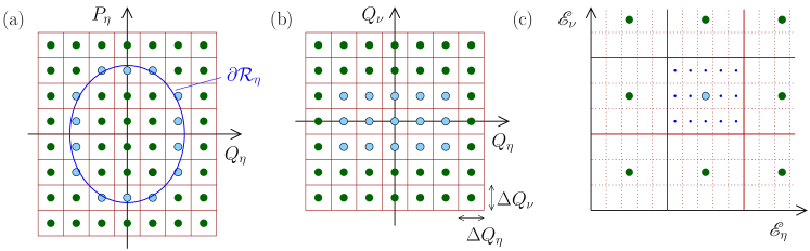
Figure 1: (a) A portion of the phase space $\mathbb{G}_{\eta}$ of mode ${\eta}$. The continuous blue ellipse, ${\partial\mathcal{R}_{\eta}}$, is a particular constant-energy path that the oscillation follows when it is decoupled from other modes. The set of pale blue and green spots is a maximal set of mutually-distinguishable microstates, $\Gamma_{\eta}$, of mode ${\eta}$. In statistical models of the mode’s microstates, each spot represents all points within its rectangular neighbourhood. (b) A portion of the microstructure space of modes ${\eta}$ and ${\nu}$. The spots belong to a maximal set of mutually distinguishable points and represent the rectangular regions they inhabit. The pale blue spots mark regions visited during the motion of the modes, assuming that their energies, ${\mathscr{E}_{\eta}}$ and ${\mathscr{E}_{\nu}}$, are constant and that neither of their frequencies, $\omega_{\eta}$ and $\omega_{\nu}$, is an integer multiple of the other. Each of the $15$ pale blue spots represents the four points ${(P_{\eta},P_{\nu},Q_{\eta},Q_{\nu})=\left(\pm\sqrt{2\mathscr{E}_{\eta}-\omega_{\eta}^{2}Q_{\eta}^{2}},\pm\sqrt{2\mathscr{E}_{\nu}-\omega_{\nu}^{2}Q_{\nu}^{2}},Q_{\eta},Q_{\nu}\right)}$ in their joint phase space ${\mathbb{G}_{\eta}\times\mathbb{G}_{\nu}}$. (c) The pale blue spot is the energy of the trajectory represented by pale blue spots in panels (a) and (b). We cannot calculate the partition function of modes ${\eta}$ and ${\nu}$ as ${\mathcal{Z}_{\eta}\mathcal{Z}_{\nu}=\sum_{\mathscr{E}_{\eta}}\sum_{\mathscr{E}_{\nu}}e^{-\beta\left(\mathscr{E}_{\eta}+\mathscr{E}_{\nu}\right)}}$ if the double summation is over a square grid in ${(\mathscr{E}_{\eta},\mathscr{E}_{\nu})}$-space. The numbers of energies sampled along each axis are only in the same ratio as the numbers of mutually-distinguishable mode coordinates along each axis in ${(Q_{\eta},Q_{\nu})}$-space, and the numbers of mutually-distinguishable points in ${\mathbb{G}_{\eta}}$ and ${\mathbb{G}_{\nu}}$, if the spacings of sampled values along the mode’s energy axes are their frequencies times the same constant.

IV.1 Oscillators and standing waves

If the potential energy of a classical dynamical system is a smooth function ${U(\mathbf{Q})}$ of its microstructure ${\mathbf{Q}}$, the system can be brought arbitrarily close to a minimum of its potential energy, ${\mathbf{Q}_{\text{min}}}$, by cooling it slowly. Once ${\norm{\mathbf{Q}-\mathbf{Q}_{\text{min}}}}$ is small enough, lowering its temperature further brings its dynamics closer to a superposition of harmonic oscillations of the normal modes of its stable equilibrium structure, ${\mathbf{Q}_{\text{min}}}$. For example, a set of mutually-attractive particles would condense into a stable vibrating cluster when cooled. The normal modes of a finite crystal or a continuous bounded medium are standing waves, so their dynamics become superpositions of standing waves when they are cold enough.

If we specify the microstructure by the set of displacements from mechanical equilibrium along the normal mode eigenvectors, each DOF $\eta$ is an oscillator or standing wave with a different angular frequency ${\omega_{\eta}}$, in general, whose energy can be expressed as

$$\mathscr{E}_{\eta}\equiv\frac{1}{2}(\dot{Q}_{\eta}^{2}+\omega_{\eta}^{2}Q_{\eta}^{2}),$$ (6)

where the mode coordinate ${Q_{\eta}}$ has the dimensions of ${\text{distance}\times\sqrt{\text{mass}}}$. In the limit ${T\to 0}$ the behaviour of the system is described perfectly by a Hamiltonian of the form

$$\mathcal{H}(\mathbf{P},\mathbf{Q}) =U(\mathbf{Q}_{\text{min}})+\frac{1}{2}\sum_{\eta}\left[P_{\eta}^{2}+\omega_{\eta}^{2}Q_{\eta}^{2}\right],$$ (7)

where ${U(\mathbf{Q}_{\text{min}})}$ is a constant that is irrelevant to the dynamics, and ${P_{\eta}\equiv\dot{Q}_{\eta}}$ is the momentum conjugate to ${Q_{\eta}}$.

As illustrated in Fig. 1, the true path ${\partial\mathcal{R}_{\eta}}$ of mode ${\eta}$ in its phase space ${\mathbb{G}_{\eta}}$ is continuous. It is only the accessible information about the path that is quantized. As discussed in Sec. III.2 and at the beginning of Sec. IV, each point ${\Gamma_{\eta}\in\partial\mathcal{R}_{\eta}}$ is indistinguishable from all points within a neighbourhood of it, whose area is $h_{\eta}$.

Uncertainty manifests differently in the microstate probability distribution depending on which set of coordinates is used to specify the microstate. Having found that $p$ is a Maxwell-Boltzmann distribution when standard position and momentum coordinates ${(P_{\eta},Q_{\eta})}$ are used, let us now perform the canonical transformation ${(P_{\eta},Q_{\eta})\mapsto(\mathcal{I}_{\eta},\vartheta_{\eta})}$, where ${(\mathcal{I}_{\eta},\vartheta_{\eta})}$ are the action-angle variables [11, 1, 10]. Then we will deduce the form of $p$ when the microstate is specfied as ${\mathbf{\Gamma}=(\mathbfcal{I},\bm{\vartheta})\equiv\left(\mathcal{I}_{1},\mathcal{I}_{2},\cdots,\vartheta_{1},\vartheta_{2},\cdots\right)}$.

The action variable is defined as

$$\mathcal{I}_{\eta}\equiv\frac{1}{2\pi}\oint_{\partial\mathcal{R}_{\eta}}P_{\eta}\differential{Q_{\eta}}=\frac{1}{2\pi}\int\int_{\mathcal{R}_{\eta}}\differential{P_{\eta}}\wedge\differential{Q_{\eta}},$$

where the first integral is performed around the closed continuous trajectory ${\partial\mathcal{R}_{\eta}}$ defined by the equation ${\mathcal{H}_{\eta}(P_{\eta},Q_{\eta})=\mathscr{E}_{\eta}}$ and depicted in Fig. 1(a). The second expression, which involves an integral over the region $\mathcal{R}_{\eta}$ enclosed by the elliptical path ${\partial\mathcal{R}_{\eta}}$, follows from the generalized Stokes theorem.

It follows from the definition of ${\mathcal{I}_{\eta}}$ that ${2\pi\mathcal{I}_{\eta}}$ is the area enclosed by ${\partial\mathcal{R}_{\eta}}$. From Eq. 6, it is easy to see that the semi-axes of ${\partial\mathcal{R}_{\eta}}$ are ${\sqrt{2\mathscr{E}_{\eta}}/\omega_{\eta}}$ and ${\sqrt{2\mathscr{E}_{\eta}}}$. Therefore, equating two expressions for the area enclosed gives

$$2\pi\mathcal{I}_{\eta}=\frac{2\pi}{\omega_{\eta}}\mathscr{E}_{\eta}\implies\mathcal{I}_{\eta}=\frac{\mathscr{E}_{\eta}}{\omega_{\eta}}.$$

The reason for choosing ${\mathcal{I}_{\eta}}$ as one of our variables should now be apparent: It allows us to express the new mode Hamiltonian as

$$\mathcal{H}_{\eta}(\vartheta_{\eta},\mathcal{I}_{\eta})=\mathcal{H}_{\eta}(\mathcal{I}_{\eta})=\mathcal{I}_{\eta}\omega_{\eta}.$$ (8)

If we now followed precisely the same procedure with the new coordinates as we used to derive the Maxwell-Boltzmann distribution in Sec. III.2, we would reach Eq. 2, with $\mathcal{Z}$ and ${\mathcal{Z}_{\eta}}$ expressed as sums over all ${\mathbf{\Gamma}\equiv(\mathbfcal{I},\bm{\vartheta})\in\mathcal{G}}$ and over all ${\Gamma_{\eta}\in\mathcal{G}_{\eta}}$, respectively. That is,

$$\mathcal{Z}=\sum_{\mathbf{\Gamma}}e^{-\beta\mathcal{H}(\mathbf{\Gamma})}=\sum_{\mathbfcal{I}}e^{-\beta\mathcal{H}(\mathbfcal{I})}=\prod_{\eta}\mathcal{Z}_{\eta},$$

where

$$\mathcal{Z}_{\eta}\equiv\sum_{\mathcal{I}_{\eta}}e^{-\beta\mathcal{H}_{\eta}(\mathcal{I}_{\eta})}=\sum_{\mathcal{I}_{\eta}}e^{-\beta\mathcal{I}_{\eta}\omega_{\eta}},$$ (9)

and the sum over ${\mathcal{I}_{\eta}}$ is over a maximal set, ${\mathcal{G}_{\eta}\equiv\Delta\mathcal{I}_{\eta}\left(\mathbb{Z}^{+}_{0}+\frac{1}{2}\right)}$, of mutually-distinguishable values of ${\mathcal{I}_{\eta}}$. The reason for the factor ${\frac{1}{2}}$ is that the lower bound ${\Delta\mathcal{I}_{\eta}}$ on the difference between mutually-distinguishable values of ${\mathcal{I}_{\eta}}$ makes all points within the interval ${[0,\frac{1}{2}\Delta\mathcal{I}_{\eta})}$ indistinguishable from zero, and makes zero indistinguishable from all points in this interval. Therefore, the sum in Eq. 9 can be viewed as ${1/\Delta\mathcal{I}_{\eta}}$ times a Riemann sum over ${\mathbb{R}^{+}}$, which samples intervals of width ${\Delta\mathcal{I}_{\eta}}$ centered at ${\frac{1}{2}\Delta\mathcal{I}_{\eta}}$, ${\frac{3}{2}\Delta\mathcal{I}_{\eta}}$, ${\frac{5}{2}\Delta\mathcal{I}_{\eta}}$, etc..

Now, since $h_{\eta}$ is a phase space area, and assuming that the magnitude of $h_{\eta}$ is the same for every DOF of every physical system, the unavoidable uncertainty in the value of ${2\pi\mathcal{I}_{\eta}}$ must be ${h_{\eta}=h_{\scriptscriptstyle?}}$, and the unavoidable uncertainty in the value of ${\mathcal{I}_{\eta}}$ must be ${\hbar_{\scriptscriptstyle?}\equiv h_{\scriptscriptstyle?}/(2\pi)}$. Therefore the partition function can be expressed as

$$\mathcal{Z}_{\eta} =\sum_{n_{\eta}\in\mathbb{Z}^{+}_{0}}e^{-\beta\left(n_{\eta}+\frac{1}{2}\right)\hbar_{\scriptscriptstyle?}\omega_{\eta}}$$

$$=\frac{e^{-\frac{1}{2}\beta\hbar_{\scriptscriptstyle?}\omega_{\eta}}}{1-e^{-\beta\hbar_{\scriptscriptstyle?}\omega_{\eta}}}=\frac{e^{\frac{1}{2}\beta\hbar_{\scriptscriptstyle?}\omega_{\eta}}}{e^{\beta\hbar_{\scriptscriptstyle?}\omega_{\eta}}-1},$$

where the second line has been reached by using the fact that the right hand side of the first line is an infinite geometric series. We can now express the free energy as

$$\mathcal{F} =-\beta^{-1}\log\mathcal{Z}=-\beta^{-1}\sum_{\eta}\log\mathcal{Z}_{\eta}$$

$$=\sum_{\eta}\left[\frac{1}{2}\hbar_{\scriptscriptstyle?}\omega_{\eta}+k_{B}T\log\left(1-e^{-\beta\hbar_{\scriptscriptstyle?}\omega_{\eta}}\right)\right].$$

The term ${\frac{1}{2}\hbar_{\scriptscriptstyle?}\omega_{\eta}}$ is commonly known as the zero point energy of mode ${\eta}$.

We can also calculate the expectation value,

$$\bar{n}_{\eta}\equiv\mathcal{Z}_{\eta}^{-1}\sum_{n_{\eta}\in\mathbb{Z}^{+}_{0}}n_{\eta}e^{-\beta\left(n_{\eta}+\frac{1}{2}\right)\hbar_{\scriptscriptstyle?}\omega_{\eta}},$$ (10)

of ${n_{\eta}}$ using Eq. 9 as follows:

$$\partialderivative{\beta}\left(\sum_{n_{\eta}\in\mathbb{Z}^{+}_{0}}e^{-\beta\left(n_{\eta}+\frac{1}{2}\right)\hbar_{\scriptscriptstyle?}\omega_{\eta}}\right)=\partialderivative{\beta}\left(\frac{e^{\frac{1}{2}\beta\hbar_{\scriptscriptstyle?}\omega_{\eta}}}{e^{\beta\hbar_{\scriptscriptstyle?}\omega_{\eta}}-1}\right).$$

After taking the derivatives and simplifying, this can be expressed as

$$\bar{n}_{\eta}=\frac{1}{e^{\beta\hbar_{\scriptscriptstyle?}\omega_{\eta}}-1}.$$

The integer ${n_{\eta}}$ is commonly referred to as the occupation number of mode ${\eta}$ and ${\bar{n}_{\eta}}$ is its thermal average.

When the modes’ amplitudes are large enough that they do interact, their energies and frequencies vary, their paths in their phase spaces are no longer elliptical, and matters become more complicated. Nevertheless, simplifying assumptions are often justified, which allow a Bose-Einstein distribution to be used as the basis for a statistical description of the system’s microstates and observables. For example, if the energy of mode ${\eta}$ is modulated by a mode ${\eta^{\prime}}$ whose frequency is sufficiently low (${\omega_{\eta^{\prime}}\ll\omega_{\eta}}$), then ${\mathcal{I}_{\eta}}$ is approximately adiabatically invariant under this modulation [11, 1, 10], and the dominant effect of the interaction on mode ${\eta}$ is to modulate its frequency.

As another example, when the interactions between modes are weak, the distribution of each mode’s energy among frequencies is broadened and shifted relative to its ${T\to 0\;}$limit. Therefore, it still has a well defined mean frequency and mean energy, which allows the Bose-Einstein distribution to be used effectively in many cases.

IV.2 Generalizations to non-oscillatory systems

I have now derived the Bose-Einstein distribution for a classical system whose dynamics is a superposition of independent harmonic oscillations. My derivation made use of two properties of the system’s Hamiltonian: The first was that it could be expressed as a sum ${\mathcal{H}=\sum_{\eta}\mathcal{H}_{\eta}}$ of the Hamiltonians $\mathcal{H}_{\eta}$ of independent DOFs. The second was that each $\mathcal{H}_{\eta}$ could be expressed as a linear function of only one variable. For oscillations, this was achieved by transforming to action-angle variables, so that each ${\mathcal{H}_{\eta}}$ took the form ${\mathcal{H}_{\eta}(\mathcal{I}_{\eta})=\mathcal{I}_{\eta}\omega_{\eta}}$. Since variations of ${\omega_{\eta}}$ are negligible when interactions are weak, ${\mathcal{I}_{\eta}}$ is effectively the only variable that appears in $\mathcal{H}_{\eta}$.

The Hamiltonians of many other kinds of physical systems, composed of mutually-noninteracting DOFs, can be transformed canonically into forms that allow the Bose-Einstein distribution to be derived. In principle it can be derived whenever there exists a curve ${\gamma_{\eta}:\mathbb{R}^{+}\to\mathbb{G}_{\eta};t\mapsto\gamma_{\eta}(t)}$ in the phase space $\mathbb{G}_{\eta}$ of each DOF such that energies of DOF $\eta$ are represented on ${\gamma_{\eta}}$ in the same proportions as they are represented in ${\mathbb{G}_{\eta}}$. To be more precise, energies should be represented on maximal samplings of ${\gamma_{\eta}}$ in the same proportions as they are represented on maximal samplings of ${\mathbb{G}_{\eta}}$.

Once each $\mathcal{H}_{\eta}$ has been transformed canonically into the form ${\mathcal{H}_{\eta}(X_{\eta})=A_{\eta}X_{\eta}+B_{\eta}}$, where ${X_{\eta}\in\mathbb{R}}$ is a continuously-varying generalized coordinate or momentum, and $A_{\eta}$ and $B_{\eta}$ are constants, the full Hamiltonian becomes

$$\mathcal{H}(\mathbf{X}) \equiv U(\mathbf{Q}_{\text{min}})+\sum_{\eta}B_{\eta}+\sum_{\eta}A_{\eta}X_{\eta}$$ (11)

where ${\mathbf{X}\equiv(X_{1},X_{2},\cdots)}$. Let ${\frac{1}{2}\Delta X_{\eta}}$ denote the smallest difference between mutually-distinguishable values of $X_{\eta}$; let ${\epsilon_{\eta}\equiv A_{\eta}\Delta X_{\eta}}$; and let ${C\equiv e^{-\beta\left(U(\mathbf{Q}_{\text{min}})+\sum_{\eta}B_{\eta}\right)}}$. Then the partition function can be expressed as

$$\mathcal{Z} =C\prod_{\eta}\sum_{n_{\eta}\in\mathbb{Z}^{+}_{0}}e^{-\beta(n_{\eta}+\frac{1}{2})\epsilon_{\eta}},$$

and it is straightforward to show that ${\bar{n}_{\eta}=1/\left(e^{\beta\epsilon_{\eta}}-1\right)}$.

One example of a system whose Hamiltonian can be transformed canonically into the form of Eq. 11 is an ideal gas. At any given point in time, its Hamiltonian has the form, ${\mathcal{H}(\mathbf{P})\equiv\sum_{\eta}\mathcal{H}_{\eta}(P_{\eta})=\frac{1}{2}\sum_{\eta}P_{\eta}^{2}}$, which is the Hamiltonian of a set of independent free particles. A free particle Hamiltonian can be transformed canonically into a harmonic oscillator Hamiltonian [6]; therefore, it can also be transformed into action-angle coordinates.

V Probability domain quantization

In this section I briefly discuss why the existence of a fundamental limit on measurement precision implies that the most informative probability distribution for the microstate of a physical system is not a probability density function, whose domain is $\mathbb{G}$, but a probability mass function whose domain is the quantized phase space $\mathcal{G}$.

Let us suppose that $M$ identical systems were prepared in macrostate $\mathcal{M}$, and that the microstate of each one was measured with the highest precision possible, i.e., each one was constrained to a region of phase space of measure $\mathbf{h}$. Then, even in the limit ${M\to\infty}$, the results of these experiments would not determine a unique probability density function ${\rho(\mathbf{\Gamma})}$ for the true microstate of a system in macrostate $\mathcal{M}$: Each microstate $\mathbf{\Gamma}_{t}$ would only be constrained to a neighbourhood of the measured value. Therefore multiple probability density functions would be consistent with the data.

For example, consider a denser partitioning of $\mathbb{G}$ than the one described in Sec. III.2: Let ${\mathcal{G}^{\scriptscriptstyle<}}$ denote a countable set of evenly-spaced points in $\mathbb{G}$, which are closer to one another than elements of $\mathcal{G}$ are, and let ${\mathcal{N}^{\scriptscriptstyle<}_{\mathbf{\Gamma}}}$ denote the set of points in $\mathbb{G}$ that are closer to ${\mathbf{\Gamma}\in\mathcal{G}^{\scriptscriptstyle<}}$ than to any other element of $\mathcal{G}^{\scriptscriptstyle<}$. Then, because ${\big{|}{\mathcal{N}^{\scriptscriptstyle<}_{\mathbf{\Gamma}}}\big{|}<\mathbf{h}}$, the empirical data would not uniquely define a probability distribution ${p^{\scriptscriptstyle<}:\mathcal{G}^{\scriptscriptstyle<}\to[0,1];\mathbf{\Gamma}\mapsto p^{\scriptscriptstyle<}_{\mathbf{\Gamma}}\equiv\Pr(\mathbf{\Gamma}_{t}\in\mathcal{N}^{\scriptscriptstyle<}_{\mathbf{\Gamma}})}$ because some measurements would be consistent with ${\mathbf{\Gamma}_{t}}$ being in more than one of the neighbourhoods in the set ${\{\mathcal{N}^{<}_{\mathbf{\Gamma}}:\mathbf{\Gamma}\in\mathcal{G}^{\scriptscriptstyle<}\}}$. By contrast, the result of any accurate measurement of ${\mathbf{\Gamma}_{t}}$, whose precision is at the fundamental limit $\mathbf{h}$, is consistent with ${\mathbf{\Gamma}_{t}}$ being in exactly one of the neighbourhoods ${\mathcal{N}_{\mathbf{\Gamma}}}$.

Therefore the distribution $p$ defined in Sec. III.1 and Sec. III.2 is both the most informative distribution that can be determined uniquely from empirical data, and the most informative empirically-unfalsifiable distribution that can be deduced theoretically. An infinite number of probability density functions ${\rho(\mathbf{\Gamma})}$ satisfy ${\int_{\mathcal{N}_{\mathbf{\Gamma}}}\rho(\mathbf{\Gamma}^{\prime})\differential{\mathbf{\Gamma}^{\prime}}=p_{\mathbf{\Gamma}}}$ for all ${\mathbf{\Gamma}\in\mathcal{G}}$; but if it was claimed that any one of them was the true microstate distribution in macrostate $\mathcal{M}$, this claim could not be falsified or validated.

The fact that ${\mathcal{G}}$ is countable does not imply that the microstates of the underlying physical system are quantized. It implies a quantization of the information contained in statistical models that possess the quality of being testable empirically. It is the domain of the microstate probability distribution that is quantized, not the system’s true trajectory.

VI Discussion

The Bose-Einstein distribution follows mathematically from probability domain quantization, and probability domain quantization is a consequence of the existence of a limit, $h_{\scriptscriptstyle?}$, on the precision with which a system’s microstate can be determined experimentally. I have argued that such a limit must exist.

If my argument and derivation are correct, it will be important to know whether my physical assumption that $h_{\scriptscriptstyle?}$ has the same value in the phase spaces of all degrees of freedom, and for all physical systems, is valid. If it is, and if ${h_{\scriptscriptstyle?}=h}$, this work might help to heal some fault lines within physical theory, such as the cosmological constant problem [15, 12].

Electromagnetic radiation mediates every interaction between an observer and what they are observing. Therefore, if light were a classical wave, and if the frequencies of all light waves were integer multiples of ${\Delta f}$, this frequency quantization would place a lower bound on the value of $h_{\scriptscriptstyle?}$. This is because the energy of a classical harmonic wave is ${Af^{2}}$, for some constant ${A}$. Therefore, if a wave of frequency $f$ was used as a probe, the smallest observable energy difference would be

$$\Delta\mathscr{E}=A\left(f+\Delta f\right)^{2}-Af^{2}=\left(2A\Delta f\right)f+\order{\Delta f^{2}},$$

which would imply that ${h_{\scriptscriptstyle?}>2A\Delta f}$.

Frequency quantization would not imply that the energy of each classical wave was quantized. It would imply that, if probability domain quantization was not recognized and accounted for, it would appear to be quantized.

While the possibility exists that my derivation is the true explanation for empirical data being consistent with Bose-Einstein statistics, we should be more open to the possibility that quantum theory is not, after all, a generalization of classical physics. We should not dismiss the possibility that, had the development of classical statistical mechanics not been slowed by the assumption that it would always be less general than quantum mechanics, it might have evolved into a state in which it shared quantum theory’s experimentally-discovered mathematical skeleton. If the mathematical structure of quantum theory had been found in this way, it would possess logical foundations.

References

- Arnold [1989] Arnold, V I (1989), Mathematical Methods of Classical Mechanics, 2nd ed., Graduate Texts in Mathematics (Springer New York).
- Bose [1924] Bose, (1924), “Plancks gesetz und lichtquantenhypothese,” Z. Phys. 26 (1), 178–181.
- Einstein [1905] Einstein, Albert (1905), “Über einen die erzeugung und verwandlung des lichtes betreffenden heuristischen gesichtspunkt,” Ann. Phys. 322 (6), 132–148.
- Einstein [1924] Einstein, Albert (1924), “Sitzungsberichte der preussischen akademie der wissenschaften,” Physikalisch-mathematische Klasse , 261.
- Einstein [1925] Einstein, Albert (1925), “Sitzungsberichte der preussischen akademie der wissenschaften,” Physikalisch-mathematische Klasse , 3.
- Glass and Scanio [1977] Glass, E N, and Joseph J. G. Scanio (1977), “Canonical transformation to the free particle,” Am. J. Phys. 45 (4), 344–346.
- Gorroochurn [2018] Gorroochurn, Prakash (2018), “The end of statistical independence: The story of Bose-Einstein statistics,” Math. Intell. 40 (3), 12–17.
- Jaynes [1957a] Jaynes, E T (1957a), “Information theory and statistical mechanics,” Phys. Rev. 106, 620–630.
- Jaynes [1957b] Jaynes, E T (1957b), “Information theory and statistical mechanics. II,” Phys. Rev. 108, 171–190.
- Lanczos [1949] Lanczos, Cornelius (1949), The Variational Principles of Mechanics, Heritage Series (University of Toronto Press).
- Landau et al. [1976] Landau, LD, E.M. Lifshitz, J.B. Sykes, and J.S. Bell (1976), Mechanics: Volume 1, Course of theoretical physics (Elsevier Science).
- Lea [2021] Lea, Rob (2021), “A new generation takes on the cosmological constant,” Phys. World 34, 42.
- Lewis [1926] Lewis, Gilbert N (1926), “The conservation of photons,” Nature 118, 874–875.
- Mehra and Rechenberg [2000] Mehra, J, and H. Rechenberg (2000), The Historical Development of Quantum Theory, Vol. I (Springer New York).
- Moskowitz [2021] Moskowitz, Clara (2021), “The cosmological constant is physics’ most embarrassing problem,” Sci. Am. 324, 23–29.
- Planck [1901] Planck, Max (1901), “Ueber das gesetz der energieverteilung im normalspectrum,” Annalen der Physik 309 (3), 553–563.
- Shannon [1948] Shannon, C E (1948), “A mathematical theory of communication,” The Bell System Technical Journal 27 (3), 379–423.