Diffusion Models for Counterfactual Generation and Anomaly Detection in Brain Images

Abstract

Segmentation masks of pathological areas are useful in many medical applications, such as brain tumour and stroke management. Moreover, healthy counterfactuals of diseased images can be used to enhance radiologists’ training files and to improve the interpretability of segmentation models. In this work, we present a weakly supervised method to generate a healthy version of a diseased image and then use it to obtain a pixel-wise anomaly map. To do so, we start by considering a saliency map that approximately covers the pathological areas, obtained with ACAT. Then, we propose a technique that allows to perform targeted modifications to these regions, while preserving the rest of the image. In particular, we employ a diffusion model trained on healthy samples and combine Denoising Diffusion Probabilistic Model (DDPM) and Denoising Diffusion Implicit Model (DDIM) at each step of the sampling process. DDPM is used to modify the areas affected by a lesion within the saliency map, while DDIM guarantees reconstruction of the normal anatomy outside of it. The two parts are also fused at each timestep, to guarantee the generation of a sample with a coherent appearance and a seamless transition between edited and unedited parts. We verify that when our method is applied to healthy samples, the input images are reconstructed without significant modifications. We compare our approach with alternative weakly supervised methods on IST-3 for stroke lesion segmentation and on BraTS2021 for brain tumour segmentation, where we improve the DICE score of the best competing method from $0.6534$ to $0.7056$.

1 Introduction

The remarkable progress in advanced imaging technologies has led to a significant enhancement in the quality of medical care for patients. These cutting-edge tools empower radiologists to achieve ever-increasing levels of accuracy when diagnosing suspicious regions such as tumors, polyps, and areas of blood rupture (Acharya et al., 1995). Moreover, physicians are now able to implement precise and carefully measured treatment methods, thanks to the invaluable support provided by these imaging technologies. Indeed, the detection of pathological markers in medical images plays an important role in diagnosing disease and monitoring its progression. However, in many cases, segmentation of the Regions of Interest (ROI) is performed manually by radiologists, making it not only an expensive process but also prone to errors and inconsistencies across different annotators  (Grünberg et al., 2017; Fontanella et al., 2020). Therefore, the development of automated ROI detection systems is a very active area of research, for its potential to save time and money, while mitigating some of the inherent biases associated with human evaluations.

When a patient is diagnosed with brain tumour, segmentation of the pathological regions is important for planning the surgical treatments, monitoring the growth of the tumour and for image-guided intervention (Ranjbarzadeh et al., 2021). In particular, Magnetic Resonance Imaging (MRI) is a widely used non-invasive technique that generates a vast array of tissue contrasts. Medical experts have extensively employed it to diagnose brain tumors. However, the normal anatomy can be severely distorted by the tumour, making it harder to plan surgical approaches that avoid key structures. For this reason, generating an equivalent healthy image could improve surgical planning by helping the identification of anatomical areas.

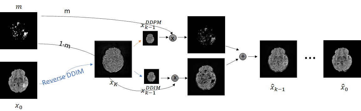
Figure 1: Our approach begins by transforming an abnormal image $\bm{x}_{0}$ into its noised version $\bm{x}_{K}$ using the reversed sampling technique of DDIMs. Subsequently, we employ DDPM sampling to modify the pathological area, identified through the saliency map generated with ACAT, aiming to restore the normal anatomical structure based on the contextual information from the surrounding regions. Meanwhile, the regions of the image that do not contain any pathological elements are restored to their original appearance using DDIM sampling. Throughout the sampling process, these two components are fused together to ensure a seamless and realistic transition between the edited and unedited parts, resulting in a final image $\bm{\hat{x}}_{0}$ with a visually coherent and natural appearance

Another clinical application in which the detection of the volume of a lesion plays an important role is stroke management. In particular, it is important in the prognostic decision, in the selection process for acute treatment (Marks et al., 1999), and in anticipating complications (Mori et al., 2001). Estimates of the tissue at risk and of the ischemic core are usually derived using Computed tomographic perfusion (CTP), perfusion-weighted imaging (PWI) or MRI diffusion-weighted imaging (DWI) (Powers et al., 2019). Software packages that automatically compute these estimates from perfusion imaging were also developed to facilitate clinical decisions about stroke treatment (Mokli et al., 2019). However, Computed Tomography (CT) scans are the most commonly used tool in stroke imaging, due to being inexpensive, efficient and widely available (Mokli et al., 2019). Consequently, quantitative measurements of the signs of infarction from CT scans, while more difficult to perform than on perfusion images, would be helpful in clinical practice.

For these reasons, we propose a weakly-supervised method that is able to automatically segment brain tumours in MRI images and stroke lesions in CT scans. In particular, we generate anomaly maps without using pixel-level annotations of the anomalies, but using exclusively image-level labels (that are needed only at training time). The same methodology could also be applied to other pixel-wise anomaly detection tasks in medical images.

Radiologists’ perception of machine learning tools varies from acceptance and enthusiasm to skepticism (Pakdemirli, 2019). Providing simple anomaly maps could be negatively received by highly trained radiologists, who could consider it demeaning to their expertise. For this reason, in our approach we remove the lesions from pathological images and generate anomaly maps based on the difference between the original image and its normal-looking version. The healthy version of the image could be provided in place, or in addition, to the anomaly map, in order to better engage with clinicians and allow them to use their own inference to detect abnormalities. Indeed, radiologists usually detect deviations from a mental representation of the normal image (Kundel et al., 1978). Having a representation of the inner workings of the automatic image segmentation tool would also increase clinicians’ trust in the model. Moreover, comparing normal and abnormal images is a common practice when teaching radiologists (Xie et al., 2020). Since normal anatomy can vary a lot, it is important for trainees to be exposed to a high number of healthy images. However, the majority of teaching files are skewed towards pathological samples (Boutis et al., 2016). Therefore, by transforming abnormal examples to match normal anatomy, we could prevent this data imbalance and aid more effective training of radiologists.

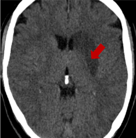
(a) Image

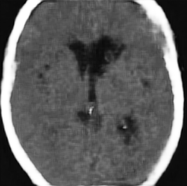
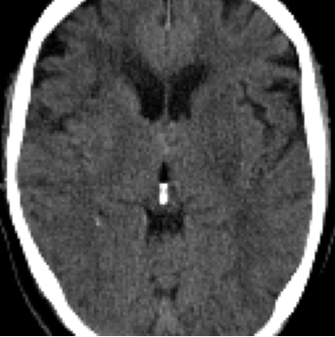
(b) f-AnoGan

(c) CG

(d) CFG

(e) ACAT

(f) Dif-fuse

Figure 2: Original image (a) and healthy counterfactuals (top row) with corresponding anomaly maps (bottom row), obtained with f-AnoGAN (b), classifier guidance (c), classifier-free guidance (d), ACAT (e) and Dif-fuse (f). ACAT generates a reasonable anomaly map, but is not able to fully remove the lesion. Dif-fuse refines the anomaly map obtained with ACAT, while at the same time creating a credible counterfactual example. The other approaches introduce artifacts and/or do not identify the pathological area correctly.

Previous work has employed autoencoders (Zimmerer et al., 2018; Chen & Konukoglu, 2018; Seeböck et al., 2016) or GANs (Schlegl et al., 2017; Keshavamurthy et al., 2021; Siddiquee et al., 2019) trained on healthy samples to map diseased images to their corresponding normal version. However, autoencoders do not always produce sharp images and do not guarantee a correct mapping to the healthy version. On the other hand, GAN training can sometimes be unstable, depend on many hyperparameters and generate poor samples (Shmelkov et al., 2018). For this reason, our approach is based on diffusion models, a class of generative models that have recently risen in popularity in the computer vision community due to their remarkable capabilities. They have been shown to achieve sample quality that is superior to the previous state-of-the-art GANs (Dhariwal & Nichol, 2021).

In (Wolleb et al., 2022), the authors employed diffusion models and classifier guidance (Dhariwal & Nichol, 2021) to recover the normal anatomy. However, the gradients that are needed to guide the sampling process have to be computed from a classifier trained on noised samples. This classifier often produces unreliable predictions, since in medical imaging the class of a sample is often determined by small details, that can be lost after only a few noising steps. For this reason, with this approach, we are not guaranteed to preserve the original structure of the sample and many details of the normal tissue can be modified.

A recent study (Fontanella et al., 2023) has introduced Adversarial Counterfactual Attention (ACAT), an approach for mapping diseased images to their healthy counterparts and identifying Regions of Interest (ROIs). In particular, to generate counterfactual examples, the authors utilise an autoencoder and a classifier trained separately to reconstruct and classify images respectively. Specifically, they determine the minimal shift in the latent space of the autoencoder that transitions the input image towards the desired target class, as determined by the classifier’s output. The authors extensively compared various counterfactual and gradient-based approaches for generating attribution maps to identify diseases in brain and lung CT scans. They demonstrated that their approach for generating saliency maps achieved the highest score in localizing the lesion location among six potential regions in brain CT scans. Moreover, it yielded the best Intersection over Union (IoU) and Dice score on lung CT scans.

While ACAT revolves around generating counterfactuals, its primary strength lies in accurately identifying pathological regions, which are subsequently employed in a classification pipeline. On the other hand, it falls short in producing credible counterfactual examples, an issue we aim to address in this study. An illustration of this phenomenon is depicted in Figure 2, where we can observe how ACAT is able to generate a saliency map that approximately identifies the pathological region (e, bottom row). However, in the counterfactual example, the lesion remains visible (e, top row). In contrast, our approach not only refines the saliency map but also generates a counterfactual image where the pathology is completely eliminated (f).

In order to do so, we exploit the saliency maps obtained with ACAT to guide the image generation process of diffusion models. We first train a Denoising Diffusion Probabilistic Model (DDPM)  (Ho et al., 2020) on healthy samples and use a combination of DDPM and Denoising Diffusion Implicit Model (DDIM)  (Song et al., 2020) sampling to remove pathological areas from the images. In particular, we first map an abnormal image to its noised version by using the reversed sampling approach of DDIMs. Then, with DDPM sampling we modify the pathological area, identified by the saliency map obtained previously, to recover the normal structure, based on the surrounding anatomical context. The parts of the image without pathological elements are mapped back to their original appearance with DDIM sampling. We fuse these two components at each step of the sampling process, so that the final resulting image has a realistic appearance, with a smooth transition between edited and unedited parts. We refer to our method as Dif-fuse.

In summary, our main contributions are: 1) we introduce a novel way to sample from diffusion models that, without needing lesion annotations, allows to modify ROIs while keeping the rest unchanged. By mixing the two components at each timestep we are also able to get a smooth transition between edited and unedited parts. This allows to generate realistic counterfactual examples of medical images and obtain anomaly maps of the pathological areas; 2) we improve the DICE score for image segmentation on BraTS 2021 from $0.6534$ of the best competing method to $0.7056$.

2 Related Work

2.1 Saliency Maps

Saliency maps are frequently utilised by researchers to gain insights into the inner workings of neural networks. They aid in the interpretation of convolutional neural network (CNN) predictions by emphasizing the significance of pixels in determining model outcomes. In (Simonyan et al., 2013), the authors employed the gradient of the target class’s score relative to the input image, while the Guided Backpropagation method (Springenberg et al., 2014) backpropagates solely positive gradients. The Integrated Gradient method (Sundararajan et al., 2017) integrates gradients between the input image and a baseline black image. Smilkov et al. (Smilkov et al., 2017) introduced SmoothGrad, which involves smoothing the gradients using a Gaussian kernel.

Grad-CAM (Selvaraju et al., 2017), which builds on the Class Activation Mapping (CAM) approach (Zhou et al., 2016), employs the gradients of the target class’s score with respect to the feature activations of the final convolutional layer to determine the importance of spatial locations. Given the popularity of this approach, modifications and improvements were later proposed in several papers. For example, Grad-CAM++ (Chattopadhay et al., 2018) introduced pixel-wise weighting of the gradients of the output with respect to a particular spatial position in the final convolutional layer. In this way, it is able to obtain a measure of the importance of each pixel in a feature map for the classification outcome. On the other hand, Score-CAM (Wang et al., 2020) takes a different approach by eliminating the dependency on gradients altogether. Instead, it calculates the weights of each activation map through a forward passing score for the target class.

2.2 Counterfactual Explanations

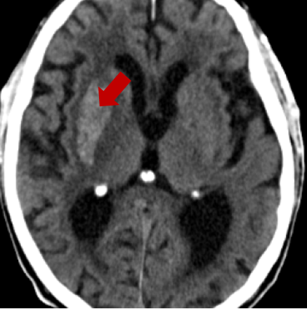
(a)

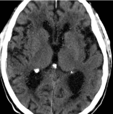
(b)

Figure 3: Input image (a) and normal image generated by applying the mask only at the end of the sampling process (b). We can observe that (b) presents some artifacts and does not have a smooth transition between edited and unedited parts.

Previous work has demonstrated that gradient-based methods for generating saliency maps have limitations. In particular, they are not reliable in identifying critical regions in medical images, as highlighted by (Eitel et al., 2019) and (Arun et al., 2021), and have been shown to be independent of model parameters and training data, as demonstrated by (Adebayo et al., 2018) and (Arun et al., 2021). As a result, techniques for visual explanations based on counterfactual examples have been developed. These methods typically involve learning a mapping between images of multiple classes to emphasize the relevant areas for each image’s respective class. The mapping is typically modeled using a CNN and trained using a GAN. In particular, Baumgartner et al. (Baumgartner et al., 2018) employed a Wasserstein GAN (Arjovsky et al., 2017). Schutte et al. (Schutte et al., 2021) trained a StyleGAN2 (Karras et al., 2020) and looked for the minimal modification in the latent space that keeps the image as close as possible to the original one, but changes the class prediction. In (Singla et al., 2021), the authors used a conditional Generative Adversarial Network (cGAN) to create a series of perturbed images that gradually display the transition between positive and negative class.

Cohen et al. (Cohen et al., 2021) proposed the latent shift method. Their approach involves training an autoencoder and a classifier as separate components: the autoencoder is responsible for reconstructing images, while the classifier focuses on image classification. Subsequently, the input images undergo perturbations in the latent space of the autoencoder, resulting in $\lambda$-shifted variations of the original image. These variations modify the probability of a particular class of interest, as determined by the classifier’s output.

In a recent study, (Fontanella et al., 2023) observed that the single-step optimisation procedure employed in the latent shift method is sometimes unable to correctly generate counterfactuals. They also note that the generated samples in the aforementioned method may deviate significantly from the original image and fail to remain on the data manifold. To address these challenges, the authors propose ACAT, an approach that enhances the optimization procedure by incorporating small progressive shifts in the latent space instead of a single-step shift of size $\lambda$ from the input image. In this way, the probability of the class of interest converges smoothly to the target value. Additionally, they introduce a regularization term to restrict the movement in latent space and ensure that the observed changes can be attributed to the class shift, while preserving the important characteristics of the image.

2.3 Anomaly Detection

The detection of disease markers in medical images is an important component for diagnosing disease and monitoring its progression. However, pixel-wise annotations are expensive to collect and often unavailable. For this reason, unsupervised or weakly-supervised anomaly detection has gained significant interest in the research community. The most popular approaches involve autoencoders, GANs, or more recently, diffusion models.

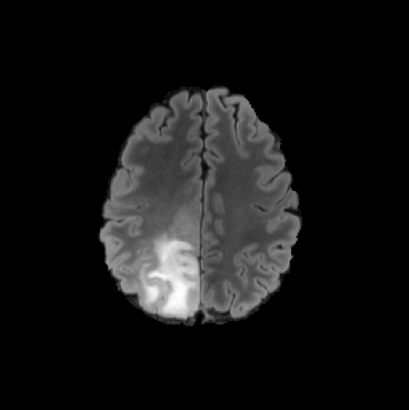
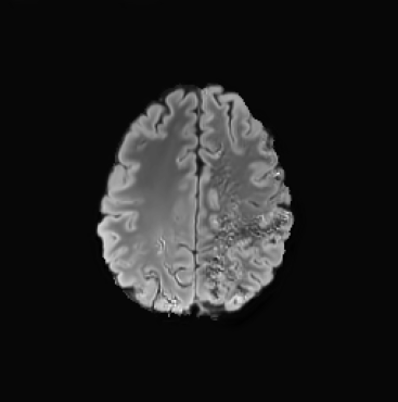
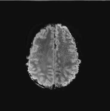
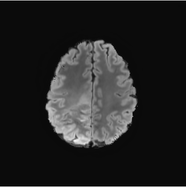
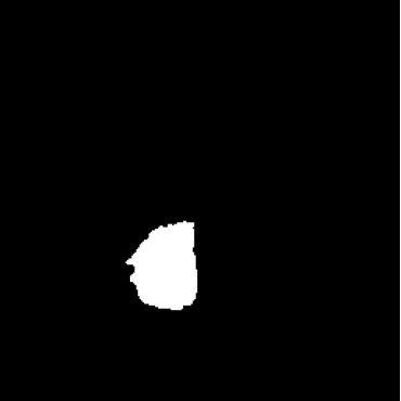
(a) Image

(b) f-AnoGan

(c) CG

(d) CFG

(e) Dif-fuse

Figure 4: Original image with ground truth segmentation mask (a) and healthy images (top row) with corresponding anomaly maps (bottom row), obtained with f-AnoGan (b), classifier guidance (c), classifier-free guidance (d) and with Dif-fuse (e). f-Ano GAN falls short in generating believable counterfactuals, whereas the approaches utilising diffusion models yield higher-quality results. However, counterfactuals generated with CG and CFG exhibit some artifacts.

A common approach when employing autoencoders is to train them to reconstruct data from healthy subjects (Zimmerer et al., 2018; Chen & Konukoglu, 2018; Seeböck et al., 2016). At test time, diseased images are mapped to the training distribution of healthy patients. The difference between the diseased input and the healthy output is the anomaly map.

Schlegl et al. (Schlegl et al., 2019) propose f-AnoGAN, which follows a similar approach but with GANs. In particular, they train a generative model and a discriminator to distinguish between generated and real data. They also propose a mapping scheme to evaluate new data at test time and identify anomalous regions. Other authors employed weakly supervised GANs, trained on both healthy and diseased images. In (Keshavamurthy et al., 2021), the authors trained a Wasserstein GAN on unpaired chest x-rays images and learned to map diseased images to healthy ones.

Diffusion models were employed in (Wolleb et al., 2022), where the authors first trained a probabilistic diffusion model on both diseased and healthy images, together with a binary classifier trained on noised samples. Then, they employed deterministic sampling from DDIM and classifier guidance (Dhariwal & Nichol, 2021) to map a diseased image into a healthy one. Another technique to guide diffusion models, proposed by (Ho & Salimans, 2022), is classifier-free guidance. During training, the label of a class-conditional diffusion model is replaced with a null label with a fixed probability. During sampling, to guide the generation process, the output of the model is extrapolated further in the direction of the desired label and away from the null label.

3 Methods

ACAT addresses the limitations of the latent shift method in generating attribution maps; however, the counterfactual examples obtained through ACAT are not entirely satisfactory. In other words, ACAT is able to identify where an image should be modified, but not exactly how to modify it to obtain a credible counterfactual. This limitation is understandable since the primary focus of their paper was to utilise these saliency maps within a classification pipeline rather than generating precise counterfactuals.

In our work, we aim to tackle this challenge by proposing a two-step approach. First, we employ ACAT to obtain initial saliency maps, which provide a rough identification of the regions requiring modification. Then, we introduce a novel sampling technique from diffusion models that enables targeted modifications to these regions while preserving the remainder of the image unchanged. By fusing both components at each timestep, we achieve a seamless transition between the edited and unedited parts, resulting in a realistic output. By considering the difference between the counterfactual example and the original image, we can also obtain the final anomaly map.

We observe that our sampling approach not only generates highly realistic counterfactuals but also enhances the initial saliency maps obtained in the first step using ACAT. This is possible because the selected regions may not undergo complete modification by the diffusion model, allowing for the preservation of healthy anatomical features identified in the initial attribution maps. A visual representation of our approach is presented in Figure 1.

In the next sections, we first give a brief overview of diffusion models, before introducing our sampling technique to generate credible counterfactuals and obtain pixel-wise anomaly maps of pathological areas in medical images.

3.1 Diffusion Models

A diffusion model is defined by a forward process that gradually adds noise to data starting from $\bm{x}_{0}\sim q(\bm{x}_{0})$ over $T$ timesteps (Ho et al., 2020):

$$q(\bm{x}_{1:T}|\bm{x}_{0})=\prod_{t=1}^{T}q(\bm{x}_{t}|\bm{x}_{t-1})$$ (1)

with $q(\bm{x}_{t}|\bm{x}_{t-1})=\mathcal{N}(\bm{x}_{t};\sqrt{1-\beta_{t}}\bm{x}_{t-1},\beta_{t}\bm{I})$

and a backward process: $p_{\theta}(\bm{x}_{0})=\int p_{\theta}(\bm{x}_{0:T})d\bm{x}_{1:T}$, where:

$$p_{\theta}(\bm{x}_{0:T}) =p(\bm{x}_{T})\prod_{t=1}^{T}p_{\theta}(\bm{x}_{t-1}|\bm{x}_{t}),\;\;$$ (2)

$$p_{\theta}(\bm{x}_{t-1}|\bm{x}_{t}) =\mathcal{N}(\bm{x}_{t-1};\bm{\mu}_{\theta}(\bm{x}_{t},t),\bm{\Sigma}_{\theta}(\bm{x}_{t},t))$$

The parameters of the forward process $\beta_{t}$ are set so that $\bm{x}_{T}$ is distributed approximately as a standard normal distribution and therefore $p(\bm{x}_{T})$ is set to a standard normal prior too. We can train the backward process to match the distribution of the forward process by optimising the evidence lower bound (ELBO): $-L_{\theta}(\bm{x}_{0})\leq log(p_{\theta}(\bm{x}_{0}))$:

$$L_{\theta}(\bm{x}_{0}) =\mathbb{E}_{q}[L_{T}(\bm{x}_{0})$$ (3)

$$+\sum_{t>1}D_{KL}(q(\bm{x}_{t-1}|\bm{x}_{t},\bm{x}_{0})||p_{\theta}(\bm{x}_{t-1}|\bm{x}_{t}))$$

$$-logp_{\theta}(\bm{x}_{0}|\bm{x}_{1})]$$

where $L_{T}(\bm{x}_{0})=D_{KL}(q(\bm{x}_{T}|\bm{x}_{0})||p(\bm{x}_{T}))$.

The forward process posteriors $q(\bm{x}_{t-1}|\bm{x}_{t},\bm{x}_{0})$ and marginals $q(\bm{x}_{t}|\bm{x}_{0})$ are Gaussian and the KL divergence can be calculated in closed form. Therefore, the diffusion model can be trained by taking stochastic gradient descent steps on random terms of Eq. (3). As noted in (Ho et al., 2020), the noising process defined in Eq. (1) allows us to sample arbitrary steps of the latents, conditioned on ${x}_{0}$. With $\alpha_{t}:=1-\beta_{t}$ and $\hat{\alpha}_{t}:=\prod_{s=0}^{t}\alpha_{s}$, we can write:

$$q(\bm{x}_{t}|\bm{x}_{0})=\mathcal{N}(\bm{x}_{t};\sqrt{\alpha_{t}}\bm{x}_{0},(1-\hat{\alpha}_{t})\bm{I}).$$ (4)

Therefore:

$$\bm{x}_{t}=\sqrt{\alpha_{t}}\bm{x}_{0}+\sqrt{(1-\hat{\alpha}_{t})}\bm{\epsilon},$$ (5)

with $\bm{\epsilon}\sim\mathcal{N}(\bm{0},\bm{I})$.

There are many ways to parametrise $\bm{\mu}_{\theta}(\bm{x}_{t},t)$ (Eq. (2)) in the prior. For example, we could predict $\bm{\mu}_{\theta}(\bm{x_{t}},t)$ with a neural network. Alternatively, we could predict $\bm{x}_{0}$ and use it to compute $\bm{\mu}_{\theta}(\bm{x_{t}},t)$. The network could also be used to predict the noise $\bm{\epsilon}$. In (Ho et al., 2020), the authors found that this option produced the best sample quality and introduced the reweighted loss function:

$$L_{\textrm{simple}}=\mathbb{E}_{t,\bm{x}_{0},\epsilon}[||\bm{\epsilon}-\bm{\epsilon}_{\theta}(\bm{x}_{t},t)||^{2}]$$ (6)

After training the diffusion model, given $\bm{X}_{T}$ sampled from $\mathcal{N}(\bm{0},\bm{I})$, we can generate a new sample $\bm{x}_{0}$, by recursively applying the sampling scheme:

$$\bm{x}_{t-1} =\sqrt{\hat{\alpha}_{t-1}}\left(\frac{\bm{x}_{t}-\sqrt{(1-\hat{\alpha}_{t})}\bm{\epsilon}_{\theta}(\bm{x}_{t},t)}{\sqrt{\hat{\alpha}_{t}}}\right)$$ (7)

$$+\sqrt{1-\hat{\alpha}_{t-1}-\sigma^{2}_{t}}\bm{\epsilon}_{\theta}(\bm{x}_{t},t)+\sigma_{t}\bm{\epsilon}$$

IN DDPMs:

$$\sigma_{t}=\sqrt{(1-\hat{\alpha}_{t-1})/(1-\hat{\alpha}_{t})}\sqrt{1-\hat{\alpha}_{t}/\hat{\alpha}_{t-1})}.$$

IN DDIMs, the stochastic component is removed by setting $\sigma_{t}=0$ and the sampling process becomes deterministic.

3.2 Dif-fuse

In our approach, we employ a DDPM trained on healthy samples and saliency maps obtained from adversarially generated counterfactual examples as in ACAT (Fontanella et al., 2023). We chose ACAT as it showed superior performance in the identification of pathological areas in brain and lung CT scans. However, in principle, saliency maps may also be generated with any other approach. Given a diseased image $\bm{x}_{0}$, we first select a noise amount $K\in[0,T]$ and map the image to its noised version $\bm{x}_{K}$ with the inverse DDIM sampling scheme proposed in (Song et al., 2020):

$$\bm{x}_{t+1} =\bm{x}_{t}+\sqrt{\hat{\alpha}_{t+1}}\Biggl{[}\Biggl{(}\sqrt{\frac{1}{\hat{\alpha}_{t}}}-\sqrt{\frac{1}{\hat{\alpha}_{t+1}}}\Biggl{)}\bm{x}_{t}$$ (8)

$$+\left(\sqrt{\frac{1}{\hat{\alpha}_{t+1}}-1}-\sqrt{\frac{1}{\hat{\alpha}_{t}}-1}\right)\bm{\epsilon}_{\theta}(\bm{x}_{t},t)\Biggl{]}$$

We then smooth the saliency map with a Gaussian kernel of size $5\times 5$ to obtain a mask $\bm{m}$. We edit the diseased regions inside the mask with DDPM sampling. Since the diffusion model was trained on normal samples, these regions are mapped to a healthy appearance. The rest of the anatomy needs to be preserved and therefore we employ DDIM sampling for the areas outside of the mask, as in Eq. (7), with $\sigma_{t}=0$. In order to obtain a coherent result, we mix the masked part with the rest of the image at each sampling step. In other words, given $\hat{\bm{x}}_{t}$, we compute:

$$\hat{\bm{x}}_{t-1}=\bm{x}^{DDPM}_{t-1}\odot\bm{m}+\bm{x}^{DDIM}_{t-1}\odot(1-\bm{m})$$ (9)

where $\odot$ is the Hadamard product. In this way, the editing process is focused on the parts that were captured by the saliency map, preventing random changes to the structural characteristics of the scan. In fact, the DDIM sampling guarantees reconstruction of the parts that don’t need to be edited. Moreover, changes to the pathological parts are performed by the DDPM considering the surrounding anatomical context. Our method is summarised in Algorithm  1.

Algorithm 1 Dif-fuse

  Input: Image $\bm{x}_{0}$, noise amount $K$, threshold value $\tau$

  Output: Counterfactual image $\hat{\bm{x}}_{0}$, anomaly map $\delta$

  Compute saliency map of $\bm{x}_{0}$ with ACAT

  Smooth the saliency map with a $5\times 5$ kernel and binarise it using the threshold $\tau$, to obtain the mask $\bm{m}$

  for all t in $[0,K-1]$ do

     $\bm{x}_{t+1}\leftarrow\bm{x}_{t}+\sqrt{\hat{\alpha}_{t+1}}\Biggl{[}\Biggl{(}\sqrt{\frac{1}{\hat{\alpha}_{t}}}-\sqrt{\frac{1}{\hat{\alpha}_{t+1}}}\Biggl{)}\bm{x}_{t}+\left(\sqrt{\frac{1}{\hat{\alpha}_{t+1}}-1}-\sqrt{\frac{1}{\hat{\alpha}_{t}}-1}\right)\bm{\epsilon}_{\theta}(\bm{x}_{t},t)\Biggl{]}$

  end for

  for all t in $[K,1]$ do

     $\hat{\bm{x}}_{t-1}\leftarrow\bm{x}^{DDPM}_{t-1}\odot\bm{m}+\bm{x}^{DDIM}_{t-1}\odot(1-\bm{m})$

  end for

  $d=|\bm{x}_{0}-\hat{\bm{x}}_{0}|$

  Apply erosion followed by dilation with a $5\times 5$ kernel to d

  Apply dilation followed by erosion to obtain the final anomaly map $\delta$

  Return: $\hat{\bm{x}}_{0}$, $\delta$

When computing $\hat{\bm{x}}_{t-1}$ with Eq. (9), the sum of the two components may not produce a perfectly coherent result. However, the incoherence is resolved by the next diffusion step, which fuses the two components better. This would not be the case if we simply computed $\hat{\bm{x}}_{0}$ with DDPM and then applied the mask only at the end of the sampling process. An illustration of this effect is presented in Figure 3, where we can observe how the normal image, generated by applying the mask solely at the conclusion of the sampling process (b), exhibits some artifacts and lacks a seamless transition between the edited and unedited regions.

In this way, we are able to obtain a normal version of the given pathological image. In order to obtain an anomaly map, we first compute the difference between the original and the generated image and then apply erosion followed by dilation with a $5\times 5$ kernel to the resulting map, in order to remove noise, and finally dilation followed by erosion, with the same kernel, to close small holes in the map.

3.3 Training details

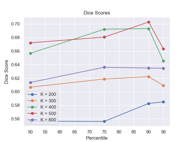
Figure 5: Dice scores obtained on the validation dataset with different combinations of thresholding percentiles to binarise the saliency maps and noise amounts K. We obtain the best result with $K=500$ and pixels in the $90^{th}$ percentile of the saliency maps.

The diffusion model is trained for 60,000 iterations, with a batch size of 10, using the loss proposed in  (Nichol & Dhariwal, 2021) and the AdamW optimiser, with learning rate of 1e-4, $\beta_{1}=0.9$, $\beta_{2}=0.999$ and weight decay coefficient of 0.05. We used an EMA rate of 0.99 and a noise schedule as in (Ho et al., 2020), setting the forward process variances to constants that increase linearly from $10^{-4}$ in the first step to $0.02$ in the last one. Training takes around two days on one NVIDIA A100 GPU. We employed 1000 sampling steps and a U-Net architecture with 128 channels in the first layer and attention heads at resolutions 8,16,32. The U-Net model employs a sequence of residual layers and downsampling convolutions, followed by another sequence of residual layers with upsampling convolutions. These layers are connected through skip connections, linking layers with the same spatial size. In particular, we used two residual blocks per resolution. Code to reproduce the experiments can be accessed at at the following url: Dif-fuse GitHub repository.

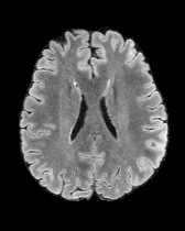
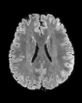
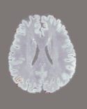
(a)

(b)

(c)

Figure 6: Healthy input images (a), images generated with Dif-fuse (b) and anomaly maps (c). We can observe that our approach obtains a good reconstruction of healthy samples.

4 Experiments

4.1 Data

We performed our experiments on IST-3 (Sandercock et al., 2011) and BraTS2021 (Baid et al., 2021) datasets.

The former is a randomised-controlled trial that collected brain imaging data, primarily CT scans, from 3035 patients exhibiting stroke symptoms. The scans were conducted at two time points: immediately after the patients’ hospital admission and again between 24-48 hours later. Radiologists involved in the trial assessed the presence or absence of early ischemic signs and recorded the location of any identified lesions for positive scans. In our analysis, we considered a total of 5681 scans, $46.31\%$ of which were classified as negative (no lesion), while the remaining scans were positive. In particular, We considered 11 slices for each scan and resized each slice to $256\times 256$. For more detailed information about the trial protocol, data collection, and the data use agreement, please refer to the following URL: IST-3 information.

The latter was collected for the Brain Tumor Segmentation (BraTS) challenge. This dataset consists of pre-operative baseline multi-parametric magnetic resonance imaging (mpMRI) scans obtained with different clinical protocols and various scanners from multiple institutions. The primary objective of the challenge is to evaluate and compare advanced techniques for segmenting different sub-regions of intrinsically heterogeneous brain glioblastomas in mpMRI scans. It includes scans in four modalities (FLAIR, T1, T1 weighted and T2). In particular, we considered the publicly available BraTS2021 training dataset, containing scans from 1251 patients. Each scan has 155 slices. However, we removed the top and bottom 25 slices, since they have minimal content, and any other empty ones, before zero padding the remaining to $256\times 256$ (from the original dimension of $240\times 240$). In the end, we are left with 131,164 slices, of which 79,113 are positive. Additional information on the dataset can be found here: BraTS2021 information.

As annotations of lesions are not available in IST-3, we utilise this dataset primarily for qualitative evaluations. On the other hand, for the BraTS2021 dataset, we have access to lesion annotations, enabling us to conduct quantitative analysis of the anomaly maps that we create. Both datasets were divided into training, validation and test sets with a 70-15-15 split.

4.2 Experimental Setup

We compare our approach with competing weakly-supervised approaches employing GANs and diffusion models. In particular, we employed f-Ano GAN (Schlegl et al., 2019), in which we train both WGAN and izi encoder for 500,000 iterations each, diffusion models with classifier guidance (CG) during sampling, following the implementation of (Wolleb et al., 2022) with noise level $K=500$ and gradient scale $s=100$, classifier-free guidance (CFG) (Ho & Salimans, 2022) with guidance scale $s^{\prime}=3$ (which in our experiments obtained the best results). As an ablation, we also consider the result obtained directly using the saliency maps obtained with ACAT, thresholded as in our approach, as anomaly maps.

In order to include the four MRI modalities available in BraTS2021 as inputs to the models, we concatenated them over the channel dimension.

4.3 Counterfactual Examples

In Figures 2 and  4 we display examples of healthy images and anomaly maps obtained with the different approaches. We can observe that f-Ano GAN is not able to generate credible counterfactuals and generally produces images of poor quality and unrealistic appearance. On the other hand, the approaches based on diffusion models are able to create more high-quality results. However, the ones obtained with CG and CFG seem to present some artifacts, which may not only impact the realism of the counterfactual examples but also the precision of the anomaly maps obtained from them. In order to better quantify the capability of these methods to accurately segment pathological areas, we compute the Dice scores of the anomaly maps they generate.

We also test our approach on healthy samples. Ideally, we would like our generative process to act as the identity function when given a normal image as input. Some examples are shown in Figure 6, where we can observe that the changes introduced by our sampling technique are relatively minimal and Dif-fuse preserves the structure and general appearance of the images.

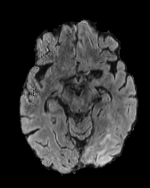
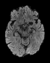
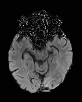
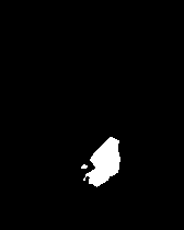
(a) Image

(b) K=250

(c) K=500

(d) K=750

Figure 7: Original image with ground truth segmentation mask (a) and healthy images (top row) with corresponding anomaly maps (bottom row), obtained with Dif-fuse with 250 (b), 500 (c), and 750 (d) noising steps. When employing lower amounts of noise, the pathological regions are not fully removed, while when the noise level is too high significant artifacts may be introduced.

4.4 Hyperparameters

In early experiments we observed that, when using the saliency maps to generate the masks needed in Dif-fuse, binarising thems produces better results. Therefore, on the validation set, we explore the optimal thresholding level for the binarisation of the saliency maps and the most appropriate noise amount to employ during the sampling from our diffusion model.

In Figure 5 we plot the dice scores obtained for different values of these hyperparameters. As we can observe, we obtain the best performance when employing 500 noising steps and selecting the pixels in the $90^{th}$ percentile of the saliency maps. In Figure 7 we display counterfactuals obtained with different noise levels. We can observe how smaller values of the noise parameter don’t allow the diffusion model to modify the image to an adequate degree, while bigger values introduce artifacts that impact the image quality of the generated image, consequently also hurting the dice score of the corresponding anomaly map.

4.5 Anomaly maps

Table 1: Dice scores on BraTS2021 test data. Dif-fuse achieves the best performance over competing weakly-supervised methods employing diffusion models or GANs and improves the results obtained with the saliency maps that are used to guide the sampling process.

Method	Dice score
f-Ano GAN	$0.5407$
Classifier guidance	$0.6534$
Classifier-free guidance	$0.6393$
ACAT	$0.5753$
Dif-fuse (Ours)	$\mathbf{0.7056}$

Having found the optimal hyperparameters, we can compute the dice scores of the anomaly maps on the test dataset. As shown in Table 1, anomaly maps obtained with Dif-fuse obtain the highest Dice score of 0.7056, improving the results obtained with f-Ano GAN (0.5407) and competing methods employing diffusion models, with classifier guidance achieving a Dice score of 0.6534 and classifier-free guidance of 0.6393. The ablation on the saliency maps obtained from ACAT (dice score of 0.5753), that are employed as part of our approach, displays how sampling from the diffusion model as in Dif-fuse is critical to obtain the best results and improve the lesion detection capability of the saliency maps.

5 Conclusion

In this work, we propose a method to remove lesions from pathological images through diffusion models, in order to generate credible counterfactuals and produce anomaly maps. To achieve this goal, we employ a two-step approach. First, we utilise ACAT to generate initial saliency maps. These maps provide a first approximation of the areas that require modification. Next, we introduce a novel way to sample from diffusion models. This technique enables us to make targeted modifications to the identified regions while preserving the remaining parts of the image. We fuse both components at each timestep to ensure a smooth transition between the edited and unedited parts and a realistic output. In particular, we modify ROIs with DDPM sampling and reconstruct the normal anatomy with DDIMs. By applying some post-processing steps to the difference between the counterfactual example and the original image, we can also obtain the final anomaly map. We observe that our sampling approach not only produces highly realistic counterfactual images but also enhances the initial saliency maps generated by ACAT in the first step. In particular, on BraTS2021, we improve the Dice score of the anomaly maps obtained with the best competing method from $0.6534$ to $0.7056$.

We applied our approach to MRI and CT scans of the brain, but we believe that it can generalise to many other medical imaging applications where image segmentation is required. We leave further testing for future work.

References

- Acharya et al. (1995) Acharya, R., Wasserman, R., Stevens, J., and Hinojosa, C. Biomedical imaging modalities: a tutorial. Computerized Medical Imaging and Graphics, 19(1):3–25, 1995.
- Adebayo et al. (2018) Adebayo, J., Gilmer, J., Muelly, M., Goodfellow, I., Hardt, M., and Kim, B. Sanity checks for saliency maps. Advances in neural information processing systems, 31, 2018.
- Arjovsky et al. (2017) Arjovsky, M., Chintala, S., and Bottou, L. Wasserstein generative adversarial networks. In International conference on machine learning, pp. 214–223. PMLR, 2017.
- Arun et al. (2021) Arun, N., Gaw, N., Singh, P., Chang, K., Aggarwal, M., Chen, B., Hoebel, K., Gupta, S., Patel, J., Gidwani, M., et al. Assessing the trustworthiness of saliency maps for localizing abnormalities in medical imaging. Radiology: Artificial Intelligence, 3(6):e200267, 2021.
- Baid et al. (2021) Baid, U., Ghodasara, S., Mohan, S., Bilello, M., Calabrese, E., Colak, E., Farahani, K., Kalpathy-Cramer, J., Kitamura, F. C., Pati, S., et al. The rsna-asnr-miccai brats 2021 benchmark on brain tumor segmentation and radiogenomic classification. arXiv preprint arXiv:2107.02314, 2021.
- Baumgartner et al. (2018) Baumgartner, C. F., Koch, L. M., Tezcan, K. C., Ang, J. X., and Konukoglu, E. Visual feature attribution using wasserstein gans. In Proceedings of the IEEE Conference on Computer Vision and Pattern Recognition, pp. 8309–8319, 2018.
- Boutis et al. (2016) Boutis, K., Cano, S., Pecaric, M., Welch-Horan, T. B., Lampl, B., Ruzal-Shapiro, C., and Pusic, M. Interpretation difficulty of normal versus abnormal radiographs using a pediatric example. Canadian medical education journal, 7(1):e68, 2016.
- Chattopadhay et al. (2018) Chattopadhay, A., Sarkar, A., Howlader, P., and Balasubramanian, V. N. Grad-cam++: Generalized gradient-based visual explanations for deep convolutional networks. In 2018 IEEE winter conference on applications of computer vision (WACV), pp. 839–847. IEEE, 2018.
- Chen & Konukoglu (2018) Chen, X. and Konukoglu, E. Unsupervised detection of lesions in brain mri using constrained adversarial auto-encoders. arXiv preprint arXiv:1806.04972, 2018.
- Cohen et al. (2021) Cohen, J. P., Brooks, R., En, S., Zucker, E., Pareek, A., Lungren, M. P., and Chaudhari, A. Gifsplanation via latent shift: a simple autoencoder approach to counterfactual generation for chest x-rays. In Medical Imaging with Deep Learning, pp. 74–104. PMLR, 2021.
- Dhariwal & Nichol (2021) Dhariwal, P. and Nichol, A. Diffusion models beat gans on image synthesis. Advances in Neural Information Processing Systems, 34:8780–8794, 2021.
- Eitel et al. (2019) Eitel, F., Ritter, K., (ADNI, A. D. N. I., et al. Testing the robustness of attribution methods for convolutional neural networks in mri-based alzheimer’s disease classification. In Interpretability of machine intelligence in medical image computing and multimodal learning for clinical decision support, pp. 3–11. Springer, 2019.
- Fontanella et al. (2020) Fontanella, A., Pead, E., MacGillivray, T., Bernabeu, M. O., and Storkey, A. Classification with a domain shift in medical imaging. Medical Imaging Meets NeurIPS Workshop, 2020.
- Fontanella et al. (2023) Fontanella, A., Antoniou, A., Li, W., Wardlaw, J., Mair, G., Trucco, E., and Storkey, A. ACAT: Adversarial counterfactual attention for classification and detection in medical imaging. In Proceedings of the 40th International Conference on Machine Learning, volume 202 of Proceedings of Machine Learning Research, pp. 10153–10169. PMLR, 23–29 Jul 2023. URL https://proceedings.mlr.press/v202/fontanella23a.html.
- Grünberg et al. (2017) Grünberg, K., Jimenez-del Toro, O., Jakab, A., Langs, G., Salas Fernandez, T., Winterstein, M., Weber, M.-A., and Krenn, M. Annotating medical image data. Cloud-Based Benchmarking of Medical Image Analysis, pp. 45–67, 2017.
- Ho & Salimans (2022) Ho, J. and Salimans, T. Classifier-free diffusion guidance. arXiv preprint arXiv:2207.12598, 2022.
- Ho et al. (2020) Ho, J., Jain, A., and Abbeel, P. Denoising diffusion probabilistic models. Advances in Neural Information Processing Systems, 33:6840–6851, 2020.
- Karras et al. (2020) Karras, T., Laine, S., Aittala, M., Hellsten, J., Lehtinen, J., and Aila, T. Analyzing and improving the image quality of stylegan. In Proceedings of the IEEE/CVF conference on computer vision and pattern recognition, pp. 8110–8119, 2020.
- Keshavamurthy et al. (2021) Keshavamurthy, K. N., Eickhoff, C., and Juluru, K. Weakly supervised pneumonia localization in chest x-rays using generative adversarial networks. Medical Physics, 48(11):7154–7171, 2021.
- Kundel et al. (1978) Kundel, H. L., Nodine, C. F., and Carmody, D. Visual scanning, pattern recognition and decision-making in pulmonary nodule detection. Investigative radiology, 13(3):175–181, 1978.
- Marks et al. (1999) Marks, M. P., Holmgren, E. B., Fox, A. J., Patel, S., von Kummer, R., and Froehlich, J. Evaluation of early computed tomographic findings in acute ischemic stroke. Stroke, 30(2):389–392, 1999.
- Mokli et al. (2019) Mokli, Y., Pfaff, J., Dos Santos, D. P., Herweh, C., and Nagel, S. Computer-aided imaging analysis in acute ischemic stroke–background and clinical applications. Neurological Research and Practice, 1(1):1–13, 2019.
- Mori et al. (2001) Mori, K., Aoki, A., Yamamoto, T., Horinaka, N., and Maeda, M. Aggressive decompressive surgery in patients with massive hemispheric embolic cerebral infarction associated with severe brain swelling. Acta neurochirurgica, 143:483–492, 2001.
- Nichol & Dhariwal (2021) Nichol, A. Q. and Dhariwal, P. Improved denoising diffusion probabilistic models. In International Conference on Machine Learning, pp. 8162–8171. PMLR, 2021.
- Pakdemirli (2019) Pakdemirli, E. Perception of artificial intelligence (ai) among radiologists. Acta radiologica open, 8(9):2058460119878662, 2019.
- Powers et al. (2019) Powers, W. J., Rabinstein, A. A., Ackerson, T., Adeoye, O. M., Bambakidis, N. C., Becker, K., Biller, J., Brown, M., Demaerschalk, B. M., Hoh, B., et al. Guidelines for the early management of patients with acute ischemic stroke: 2019 update to the 2018 guidelines for the early management of acute ischemic stroke: a guideline for healthcare professionals from the american heart association/american stroke association. Stroke, 50(12):e344–e418, 2019.
- Ranjbarzadeh et al. (2021) Ranjbarzadeh, R., Bagherian Kasgari, A., Jafarzadeh Ghoushchi, S., Anari, S., Naseri, M., and Bendechache, M. Brain tumor segmentation based on deep learning and an attention mechanism using mri multi-modalities brain images. Scientific Reports, 11(1):1–17, 2021.
- Sandercock et al. (2011) Sandercock, P. A., Niewada, M., and Członkowska, A. The international stroke trial database. Trials, 12(1):1–7, 2011.
- Schlegl et al. (2017) Schlegl, T., Seeböck, P., Waldstein, S. M., Schmidt-Erfurth, U., and Langs, G. Unsupervised anomaly detection with generative adversarial networks to guide marker discovery. In Information Processing in Medical Imaging: 25th International Conference, IPMI 2017, Boone, NC, USA, June 25-30, 2017, Proceedings, pp. 146–157. Springer, 2017.
- Schlegl et al. (2019) Schlegl, T., Seeböck, P., Waldstein, S. M., Langs, G., and Schmidt-Erfurth, U. f-anogan: Fast unsupervised anomaly detection with generative adversarial networks. Medical image analysis, 54:30–44, 2019.
- Schutte et al. (2021) Schutte, K., Moindrot, O., Hérent, P., Schiratti, J.-B., and Jégou, S. Using stylegan for visual interpretability of deep learning models on medical images. arXiv preprint arXiv:2101.07563, 2021.
- Seeböck et al. (2016) Seeböck, P., Waldstein, S., Klimscha, S., Gerendas, B. S., Donner, R., Schlegl, T., Schmidt-Erfurth, U., and Langs, G. Identifying and categorizing anomalies in retinal imaging data. arXiv preprint arXiv:1612.00686, 2016.
- Selvaraju et al. (2017) Selvaraju, R. R., Cogswell, M., Das, A., Vedantam, R., Parikh, D., and Batra, D. Grad-cam: Visual explanations from deep networks via gradient-based localization. In Proceedings of the IEEE international conference on computer vision, pp. 618–626, 2017.
- Shmelkov et al. (2018) Shmelkov, K., Schmid, C., and Alahari, K. How good is my gan? In Proceedings of the European conference on computer vision (ECCV), pp. 213–229, 2018.
- Siddiquee et al. (2019) Siddiquee, M. M. R., Zhou, Z., Tajbakhsh, N., Feng, R., Gotway, M. B., Bengio, Y., and Liang, J. Learning fixed points in generative adversarial networks: From image-to-image translation to disease detection and localization. In Proceedings of the IEEE/CVF international conference on computer vision, pp. 191–200, 2019.
- Simonyan et al. (2013) Simonyan, K., Vedaldi, A., and Zisserman, A. Deep inside convolutional networks: Visualising image classification models and saliency maps. arXiv preprint arXiv:1312.6034, 2013.
- Singla et al. (2021) Singla, S., Pollack, B., Wallace, S., and Batmanghelich, K. Explaining the black-box smoothly-a counterfactual approach. arXiv preprint arXiv:2101.04230, 2021.
- Smilkov et al. (2017) Smilkov, D., Thorat, N., Kim, B., Viégas, F., and Wattenberg, M. Smoothgrad: removing noise by adding noise. arXiv preprint arXiv:1706.03825, 2017.
- Song et al. (2020) Song, J., Meng, C., and Ermon, S. Denoising diffusion implicit models. arXiv preprint arXiv:2010.02502, 2020.
- Springenberg et al. (2014) Springenberg, J. T., Dosovitskiy, A., Brox, T., and Riedmiller, M. Striving for simplicity: The all convolutional net. arXiv preprint arXiv:1412.6806, 2014.
- Sundararajan et al. (2017) Sundararajan, M., Taly, A., and Yan, Q. Axiomatic attribution for deep networks. In International conference on machine learning, pp. 3319–3328. PMLR, 2017.
- Wang et al. (2020) Wang, H., Wang, Z., Du, M., Yang, F., Zhang, Z., Ding, S., Mardziel, P., and Hu, X. Score-cam: Score-weighted visual explanations for convolutional neural networks. In Proceedings of the IEEE/CVF conference on computer vision and pattern recognition workshops, pp. 24–25, 2020.
- Wolleb et al. (2022) Wolleb, J., Bieder, F., Sandkühler, R., and Cattin, P. C. Diffusion models for medical anomaly detection. In Medical Image Computing and Computer Assisted Intervention–MICCAI 2022: 25th International Conference, Singapore, September 18–22, 2022, Proceedings, Part VIII, pp. 35–45. Springer, 2022.
- Xie et al. (2020) Xie, Y., Chen, M., Kao, D., Gao, G., and Chen, X. Chexplain: enabling physicians to explore and understand data-driven, ai-enabled medical imaging analysis. In Proceedings of the 2020 CHI Conference on Human Factors in Computing Systems, pp. 1–13, 2020.
- Zhou et al. (2016) Zhou, B., Khosla, A., Lapedriza, A., Oliva, A., and Torralba, A. Learning deep features for discriminative localization. In Proceedings of the IEEE conference on computer vision and pattern recognition, pp. 2921–2929, 2016.
- Zimmerer et al. (2018) Zimmerer, D., Kohl, S. A., Petersen, J., Isensee, F., and Maier-Hein, K. H. Context-encoding variational autoencoder for unsupervised anomaly detection. arXiv preprint arXiv:1812.05941, 2018.