Incorporating Recklessness to Collaborative Filtering based Recommender Systems

Abstract

Recommender systems that include some reliability measure of their predictions tend to be more conservative in forecasting, due to their constraint to preserve reliability. This leads to a significant drop in the coverage and novelty that these systems can provide. In this paper, we propose the inclusion of a new term in the learning process of matrix factorization-based recommender systems, called recklessness, which enables the control of the risk level desired when making decisions about the reliability of a prediction. Experimental results demonstrate that recklessness not only allows for risk regulation but also improves the quantity and quality of predictions provided by the recommender system.

Keywords: Recommender systems, collaborative filtering, recklessness.

1 Introduction

RS have become a powerful tool for an internet-based society in recent years. Their main purpose is to provide users with a series of products or services that may be of interest to them based on their past preferences. Therefore, Recommender Systems have applications in fields such as e-commerce [10, 3], online entertainment platforms [22, 8, 9], or smart home automation [29, 19], to name a few examples.

Due to their popularity, research on RSs has grown significantly in the last decade. Most of these studies have focused on improving the quantitative aspects of the predictions generated by the artificial intelligence models on which RSs are based [34, 20]. However, there are also other studies that aim to improve the qualitative aspects of these systems [5, 18].

A recent study [27] provides a significant change in the operation of Collaborative Filtering (CF) based RSs, the most popular type of RS [7]. Traditionally, CF has approached the calculation of its predictions as a regression problem. However, most datasets used to train CF have a discrete rating system (for example, from 1 to 5 stars), and therefore, predictions should be modeled as a classification problem.

This change means that the predictions of a CF based RSs are no longer real numbers but discrete probability distributions that represent how likely a user is to rate an item with a score. For example, instead of predicting that item $i$ will interest user $u$ with 4.33 stars, a classification-based recommendation system returns the probability <0, 0, 0, 0.66, 0.34>, assuming that the possible score range is from 1 to 5 stars. For this reason, these RSs are known as probability-based RS.

Thanks to this new form of prediction, it is possible to know the reliability of a prediction: Following the previous example, we will know that a prediction of <0, 0, 0, 0, 1> is much more reliable than one of <0.19, 0.2, 0.2, 0.2, 0.21>, even though they have the same mode. By using this reliability, it is possible to gauge the output of a RS to offer more reliable predictions at the expense of sacrificing less reliable ones. In other words, the quantity and quality of predictions can be balanced by setting a threshold from which a prediction is considered not reliable enough. However, this mechanism also leads to an undesired effect: the system tends to output almost-flat predictions, with small deviations from the uniform distribution, and only a few clear items are distinguished with a more spiky distribution. This produces a more conservative system that, even with very small thresholds, suffers a noticeable drop in the coverage of items to be recommended.

To address this problem, in this paper we propose the inclusion of a new regularization term in the cost function of CF models driven by probability-based RS, called recklessness, which aims to force the model to find solutions with higher quality predictions or a greater number of predictions. This is a hyper-parameter of the system that impacts the training process of the RS fostering non-uniform distributions with higher peaks. Empirical results show that, gauging properly this hyper-parameter, we can push the Pareto front to get better predictors, both in terms of coverage and accuracy.

The rest of the article is structured as follows: Section 2 dives into the related work, Section 3 formalizes the new recklessness regularization proposed in this manuscript, Section 4 shows the experimental results of the proposed regularization, and section 5 presents the conclusions and future work of this research.

2 Related Work

Probability-based RS have sparked the interest of the research community in recent years. As mentioned in the previous section, the most representative work in this area is [27], where the authors propose encoding user ratings using one-hot encoding and then factorizing the CF voting matrix based on the Bernoulli distribution. In the same vein, the authors suggest DirMF [23], another matrix factorization model but based on the Dirichlet distribution instead of Bernoulli. OrdRec [21] proposes a model that produces user-item scores converted into probabilities over an ordinal set of ratings. URP [24] introduces another probability-based recommendation system encoded as a generative latent variable model for rating-based collaborative filtering. Finally, [6] presents a collaborative filtering approach based on artificial neural networks, adding a softmax output layer to provide probabilities instead of numerical predictions.

The increased interest in probability-based RS lies in the reliability associated with each computed prediction. The reliability of RS has been extensively studied. On one hand, some authors aim to add value to the reliability of individual predictions. For example, [1, 2] employ reliability to address the issue of voting matrix sparsity in CF, while [4] suggests using reliability to detect shilling attacks in RS. On the other hand, the overall reliability of RS is also investigated. In this regard, [25] explores the mood sensitivity aspect of truth discovery to build a reliable RS, [16] develops a reliable and private RS for applying CF in medical environments, and [35] considers utilizing user reputation to resist malicious users and ensure the recommendation’s reliability.

As mentioned earlier, this article aims to provide RS with a mechanism that allows adjusting the reliability of their predictions. To achieve this, a new hyper-parameter is introduced into the model’s learning process. A key point of this work is that the new hyper-parameter is understandable for humans. As we will see later on, positive values provide RS with less reliable predictions, whereas negative values provide more reliable predictions. This fact allows humanizing the RS and assisting their end-users. Humanizing Artificial Intelligence (AI) [17, 30] is one of the major challenges faced by science and would help address its application in medical [13], ethical [31] and customer service [32] issues, among others.

3 Recklessness Regularization

The general setup of a probability-based RS is the following. Suppose that our system contains $U$ users and $I$ items, so that we can collect their ratings in a (highly) sparse matrix $R=(r_{ui})$ of order $U\times I$, where $r_{ui}$ is the rating that the user $u$ assigned to the item $i$. Here, $r_{ui}$ belongs to some finite set $\Omega$ of possible ratings (typically, $\Omega=\{1,\ldots,5\}$ for $5$-point scales or $\Omega=\{0,1\}$ for like/dislike ratings). If the rating of the user $u$ to the item $i$ is missing, we will denote it by $r_{ui}=\bullet$.

In this setting, a probability-based RS is a function that, to any user-item pair $(u,i)$, assigns a probability distribution $\hat{\mathbb{P}}_{ui}$ on $\Omega$, seen as a sample space. In this sense, $\hat{\mathbb{P}}_{ui}(s)\in[0,1]$ should be thought as the estimation of the probability that the user $u$ assigns to item $i$ a rating $s$. From this probability, the prediction $\hat{r}_{ui}\in\Omega$ can be computed as the mode of this distribution, and its reliability $\hat{\rho}_{ui}\in[0,1]$ as the probability of this mode. In this fashion, if we set a reliability threshold $0\leq\theta\leq 1$, no prediction is issued if $\hat{\rho}_{ui}\leq\theta$.

However, more sophisticated statistics of the estimated probability $\hat{\mathbb{P}}_{ui}$ can be calculated. In particular, we can consider a random variable $X:\Omega\to\mathbb{R}$ and compute the variance $\mathbb{V}^{X}_{\hat{\mathbb{P}}_{ui}}=\mathbb{E}(X^{2})-\mathbb{E}(X)^{2}$ of this random variable. For applications, typically the set $\Omega$ of possible scores is a set of finitely many numbers $\Omega=\{x_{1},\ldots,x_{s}\}$ (for instance $\Omega=\{1,2,3,4,5\}$ in MovieLens [14]), and we can take $X:\Omega\to\mathbb{R}$ to be the identity map $X(x_{i})=x_{i}$. In this case, its variance is given by

$$\mathbb{V}^{X}_{\hat{\mathbb{P}}_{ui}}=\mathbb{E}(X^{2})-\mathbb{E}(X)^{2}=\sum_{k=1}^{s}x_{k}^{2}\hat{\mathbb{P}}_{ui}(x_{k})-\left(\sum_{k=1}^{s}x_{k}\hat{\mathbb{P}}_{ui}(x_{k})\right)^{2}.$$

Now, let us suppose that the estimated probability $\hat{\mathbb{P}}_{ui}=\hat{\mathbb{P}}_{ui}(p_{u},q_{i})$ depends on some parameters $p_{u},q_{i}\in\mathbb{R}^{D}$ associated to each user $u$ and item $i$. In the field of RSs, these parameters are typically referred to as the hidden factors. Let us collect these parameters by columns into matrices $P=(p_{1}\,|\,\ldots\,|\,p_{U})$ and $Q=(q_{1}\,|\,\ldots\,|\,q_{I})$ of sizes $D\times U$ and $D\times I$, respectively.

To train these parameters, a cost function $\mathcal{F}:\mathbb{R}^{D\times U}\times\mathbb{R}^{D\times I}\to\mathbb{R}$ is sought to be optimized so that the optimal parameters are

$$(P^{*},Q^{*})=\underset{P,Q}{\textrm{argmin}}\,\mathcal{F}(P,Q).$$

This optimal point is searched using some classical optimization algorithm such as stochastic gradient descent. Once computed this minimum, if $P^{*}=(p_{u}^{*})$ and $Q^{*}=(q_{i}^{*})$, the estimated probability distribution for a pair $(u,i)$ is $\hat{\mathbb{P}}_{u,i}(p_{u}^{*},q_{i}^{*})$.

Our proposal in this work is to modify this cost function to take into account the variance of the predicted distribution obtained. In this way, fixed a real value $\alpha\geq 0$, we define the modified cost function

$$\mathcal{F}_{\alpha}(P,Q)=\mathcal{F}(P,Q)-\alpha\sum_{u,i}\hat{\mathbb{V}}^{X}_{\hat{\mathbb{P}}_{u,i}(p_{u}^{*},q_{i}^{*})}.$$

In the case that the random variable $X:\Omega=\{x_{1},\ldots,x_{s}\}\to\mathbb{R}$ is the identity map, then

$$\mathcal{F}_{\alpha}(P,Q)=\mathcal{F}(P,Q)-\alpha\sum_{u,i}\left(\sum_{k=1}^{s}x_{k}^{2}\hat{\mathbb{P}}_{ui}(x_{k})-\left(\sum_{k=1}^{s}x_{k}\hat{\mathbb{P}}_{ui}(x_{k})\right)^{2}\right)$$

Observe that, the larger the value of $\alpha$, the more important will be to maximize the variance of the output. In this manner, large values of $\alpha$ will tend to provide estimated probability distributions $\hat{\mathbb{P}}_{ui}$ with a large variance. In other words, the algorithm is forced to return a spiky output distribution, with sharp maxima and minima. In this sense, we are impelling the method to take a risk and to stress the mode of the distribution. For this reason, we shall refer to $\alpha$ as the recklessness parameter.

To minimize it, we shall follow a stochastic gradient descend on items and users. A straightforward calculation shows that the derivatives are given by

$$\partial_{p_{u}}\mathcal{F}_{\alpha}= \;\partial_{p_{u}}\mathcal{F}-\alpha\sum_{i,k}x_{k}^{2}\partial_{p_{u}}\hat{\mathbb{P}}_{ui}(x_{k})+2\alpha\sum_{i}\left(\sum_{k}x_{k}\hat{\mathbb{P}}_{ui}(x_{k})\right)\left(\sum_{k}x_{k}\partial_{p_{u}}\hat{\mathbb{P}}_{ui}(x_{k})\right),$$

$$\partial_{q_{i}}\mathcal{F}_{\alpha}= \;\partial_{q_{i}}\mathcal{F}-\alpha\sum_{u,k}x_{k}^{2}\partial_{q_{i}}\hat{\mathbb{P}}_{ui}(x_{k})+2\alpha\sum_{u}\left(\sum_{k}x_{k}\hat{\mathbb{P}}_{ui}(x_{k})\right)\left(\sum_{k}x_{k}\partial_{q_{i}}\hat{\mathbb{P}}_{ui}(x_{k})\right).$$

Here $\partial_{p_{u}}\mathcal{F}$ and $\partial_{q_{i}}\mathcal{F}$ are the gradients of the standard cost function of the given algorithm.

Therefore, the modified update rules for stochastic gradient descend with learning rate $\eta>0$ for the pair user-item $(u,i)$ with $r_{ui}\neq\bullet$ are

$$p_{u}\leftarrow \;p_{u}-\eta\partial_{p_{u}}\mathcal{F}+\alpha\eta\sum_{k}x_{k}^{2}\partial_{p_{u}}\hat{\mathbb{P}}_{ui}(x_{k})-2\alpha\eta\left(\sum_{k}x_{k}\hat{\mathbb{P}}_{ui}(x_{k})\right)\left(\sum_{k}x_{k}\partial_{p_{u}}\hat{\mathbb{P}}_{ui}(x_{k})\right),$$

$$q_{i}\leftarrow \;q_{i}-\eta\partial_{q_{i}}\mathcal{F}+\alpha\eta\sum_{k}x_{k}^{2}\partial_{q_{i}}\hat{\mathbb{P}}_{ui}(x_{k})-2\alpha\eta\left(\sum_{k}x_{k}\hat{\mathbb{P}}_{ui}(x_{k})\right)\left(\sum_{k}x_{k}\partial_{q_{i}}\hat{\mathbb{P}}_{ui}(x_{k})\right).$$

To relate this with the usual RS models, the standard procedure is to suppose that $\hat{\mathbb{P}}_{ui}$ has some prescribed distribution, such as a normal distribution [26], a (multiple) Bernoulli distribution [27], the Dirichlet distribution [23] or a restricted binomial distribution [11]. In this manner, the cost function $\mathcal{F}$ is given by the minus log-likelihood of the known ratings

$$\mathcal{F}(P,Q)=-\log\mathcal{L}(P,Q)=-\log\prod_{r_{ui}\neq\bullet}\hat{\mathbb{P}}_{ui}(r_{ui})=-\sum_{r_{ui}\neq\bullet}\log\hat{\mathbb{P}}_{ui}(r_{ui}).$$

In this way, the recklessness cost function would be

$$\mathcal{F}_{\alpha}(P,Q)=-\sum_{r_{ui}\neq\bullet}\log\hat{\mathbb{P}}_{ui}(r_{ui})-\alpha\sum_{u,i,k}x_{k}^{2}\hat{\mathbb{P}}_{ui}(x_{k})+\alpha\left(\sum_{u,i,k}x_{k}\hat{\mathbb{P}}_{ui}(x_{k})\right)^{2}.$$

Here, recall that the dependence of this function on the parameters $P$ and $Q$ is in the predicted probability $\hat{\mathbb{P}}_{ui}=\hat{\mathbb{P}}_{ui}(p_{u},q_{i})$. In this way, the usual gradients of the standard cost function is given by

$$\partial_{p_{u}}\mathcal{F}=-\sum_{r_{ui}\neq\bullet}\frac{\partial_{p_{u}}\hat{\mathbb{P}}_{ui}(r_{ui})}{\hat{\mathbb{P}}_{ui}(r_{ui})},\quad\partial_{q_{i}}\mathcal{F}=-\sum_{r_{ui}\neq\bullet}\frac{\partial_{q_{i}}\hat{\mathbb{P}}_{ui}(r_{ui})}{\hat{\mathbb{P}}_{ui}(r_{ui})}.$$

Furthermore, if we suppose that the parameters of this distribution depend on the latent factors $p_{u}$ and $q_{i}$ through the inner product $p_{u}\cdot q_{i}$, we have that $\hat{\mathbb{P}}_{u,i}(x)=f_{x}(p_{u}\cdot q_{i})$ for some function $f$ depending on the sample $x$. Therefore, the corresponding updating rules for a pair $(u,i)$ with $r_{ui}\neq\bullet$ are

$$p_{u}\leftarrow \;p_{u}+\eta\frac{\partial_{p_{u}}\hat{\mathbb{P}}_{ui}(r_{ui})}{\hat{\mathbb{P}}_{ui}(r_{ui})}+\alpha\eta\sum_{k}x_{k}^{2}f^{\prime}_{x_{k}}(p_{u}\cdot q_{i})q_{i}$$

$$-2\alpha\eta\left(\sum_{k}x_{k}f_{x_{k}}(p_{u}\cdot q_{i})\right)\left(\sum_{k}x_{k}f^{\prime}_{x_{k}}(p_{u}\cdot q_{i})q_{i}\right),$$

$$q_{i}\leftarrow \;q_{i}+\eta\frac{\partial_{q_{i}}\hat{\mathbb{P}}_{ui}(r_{ui})}{\hat{\mathbb{P}}_{ui}(r_{ui})}+\alpha\eta\sum_{k}x_{k}^{2}f^{\prime}_{x_{k}}(p_{u}\cdot q_{i})p_{u}$$

$$-2\alpha\eta\left(\sum_{k}x_{k}f_{x_{k}}(p_{u}\cdot q_{i})\right)\left(\sum_{k}x_{k}f^{\prime}_{x_{k}}(p_{u}\cdot q_{i})p_{u}\right).$$

4 Experimental Evaluation

In this section, we present the experimental results that verify the influence of the proposed recklessness regularization on probability-based (RS). Specifically, the experiments will be conducted using the Bernoulli Matrix Factorization (BeMF) [27] recommendation model. This model has been chosen as the probability-based RS that provides the most accurate predictions.

As defined in the previous section, to incorporate recklessness regularization into a probability-based RS, it is necessary to modify its cost function. In the case of BeMF, it is based on parameters $P=(p_{u}^{k})$ for each user $u$ and possible rating $x_{k}$ and $Q=(q_{i}^{k})$ for each item $i$ and rating $x_{k}$. Therefore, as proposed in [27], the standard cost function without recklessness regularization for BeMF is

$$\mathcal{F}(P,Q)=-\sum_{r_{ui}=x_{k}}\log(\sigma(p_{u}^{k}\cdot q_{i}^{k}))-\sum_{r_{ui}\neq x_{k},\bullet}\log(1-\sigma(p_{u}^{k}\cdot q_{i}^{k})),$$

where $\sigma:\mathbb{R}\to[0,1]$, $\sigma(x)=(1+e^{-x})^{-1}$ is the logistic function. The predicted probability is thus

$$\hat{\mathbb{P}}_{ui}(x_{k})=\textrm{sm}_{k}(p_{u}^{1}\cdot q_{i}^{1},\ldots,p_{u}^{n}\cdot q_{i}^{n})=\frac{\sigma(p_{u}^{k}\cdot q_{i}^{k})}{\sum_{l}\sigma(p_{u}^{l}\cdot q_{i}^{l})},$$

where $\textrm{sm}_{k}(s_{1},\ldots,s_{n})=\sigma(s_{k})/\sum_{l}\sigma(s_{l})$ is the $k$-th entry of the softmax function. To simplify notation, we shall denote $\textrm{sm}_{k}(p_{u}\cdot q_{i})=\textrm{sm}_{k}(p_{u}^{1}\cdot q_{i}^{1},\ldots,p_{u}^{n}\cdot q_{i}^{n})$

In this way, if we modify the cost function with the recklessness parameter $\alpha$ we get

$$\mathcal{F}_{\alpha}(P,Q)= \,-\sum_{r_{ui}=x_{k}}\log(\sigma(p_{u}^{k}\cdot q_{i}^{k}))-\sum_{r_{ui}\neq x_{k},\bullet}\log(1-\sigma(p_{u}^{k}\cdot q_{i}^{k}))$$

$$-\alpha\sum_{u,i,k}x_{k}^{2}\textrm{sm}_{k}(p_{u}\cdot q_{i})+\alpha\left(\sum_{u,i,k}x_{k}\textrm{sm}_{k}(p_{u}\cdot q_{i})\right)^{2}.$$

As shown in [27], the corresponding gradients for the standard cost function are given by

$$\partial_{p_{u}^{k}}\mathcal{F}(P,Q)= -\sum_{r_{u,i}=x_{k}}{(1-\sigma(p_{u}^{k}\cdot q_{i}^{k}))}q_{i}^{k}+\sum_{r_{u,i}\neq x_{k},\bullet}{\sigma(p_{u}^{k}\cdot q_{i}^{k})}q_{i}^{k},$$

$$\partial_{q_{u}^{k}}\mathcal{F}(P,Q)= -\sum_{r_{u,i}=x_{k}}{(1-\sigma(p_{u}^{k}\cdot q_{i}^{k}))}p_{u}^{k}+\sum_{r_{u,i}\neq x_{k},\bullet}{\sigma(p_{u}^{k}\cdot q_{i}^{k})}p_{u}^{k}.$$

Therefore, the gradients for the recklessness cost function are

$$\partial_{p_{u}^{k}}\mathcal{F}_{\alpha}(P,Q)= -\sum_{r_{u,i}=x_{k}}{(1-\sigma(p_{u}^{k}\cdot q_{i}^{k}))}q_{i}^{k}+\sum_{r_{u,i}\neq x_{k},\bullet}{\sigma(p_{u}^{k}\cdot q_{i}^{k})}q_{i}^{k}$$

$$\quad+\alpha\eta\sum_{i,t}x_{t}^{2}\partial_{k}\textrm{sm}_{t}(p_{u}\cdot q_{i})q_{i}^{t}$$

$$\quad-2\alpha\eta\sum_{i}\left(\sum_{t}x_{t}\textrm{sm}_{t}(p_{u}\cdot q_{i})\right)\left(\sum_{t}x_{t}\partial_{k}\textrm{sm}_{t}(p_{u}\cdot q_{i})q_{i}^{t}\right),$$

$$\partial_{q_{i}^{k}}\mathcal{F}_{\alpha}(P,Q)= -\sum_{r_{u,i}=x_{k}}{(1-\sigma(p_{u}^{k}\cdot q_{i}^{k}))}p_{u}^{k}+\sum_{r_{u,i}\neq x_{k},\bullet}{\sigma(p_{u}^{k}\cdot q_{i}^{k})}p_{u}^{k}$$

$$\quad+\alpha\eta\sum_{u,t}x_{t}^{2}\partial_{k}\textrm{sm}_{t}(p_{u}\cdot q_{i})p_{u}^{t}$$

$$\quad-2\alpha\eta\sum_{u}\left(\sum_{t}x_{t}\textrm{sm}_{t}(p_{u}\cdot q_{i})\right)\left(\sum_{t}x_{t}\partial_{k}\textrm{sm}_{t}(p_{u}\cdot q_{i})p_{u}^{t}\right).$$

where recall that $\textrm{sm}_{t}(p_{u}\cdot q_{i})=\sigma(p_{u}^{t}\cdot q_{i}^{t})/{\sum_{l}\sigma(p_{u}^{l}\cdot q_{i}^{l})}$ is the softmax function and $\partial_{k}\textrm{sm}_{t}(p_{u}\cdot q_{i})=\textrm{sm}_{t}(p_{u}\cdot q_{i})\left(\delta_{tk}-\textrm{sm}_{k}(p_{u}\cdot q_{i})\right)$, being $\delta_{tk}=1$ if $t=k$ and $\delta_{tk}=0$ if $t\neq k$.

Hence, the updating rule for a pair user-item $(u,i)$ with $r_{ui}=x_{k}$ are

$$p_{u}^{k}\leftarrow p_{u}^{k}+(1-\sigma(p_{u}^{k}\cdot q_{i}^{k}))q_{i}^{k}-\alpha\eta\sum_{t}x_{t}^{2}\partial_{k}\textrm{sm}_{t}(p_{u}\cdot q_{i})q_{i}^{t}$$

$$\quad+2\alpha\eta\left(\sum_{t}x_{t}\textrm{sm}_{t}(p_{u}\cdot q_{i})\right)\left(\sum_{t}x_{t}\partial_{k}\textrm{sm}_{t}(p_{u}\cdot q_{i})q_{i}^{t}\right),$$

$$q_{i}^{k}\leftarrow q_{i}^{k}+(1-\sigma(p_{u}^{k}\cdot q_{i}^{k}))p_{u}^{k}-\alpha\eta\sum_{t}x_{t}^{2}\partial_{k}\textrm{sm}_{t}(p_{u}\cdot q_{i})p_{u}^{t}$$

$$\quad+2\alpha\eta\left(\sum_{t}x_{t}\textrm{sm}_{t}(p_{u}\cdot q_{i})\right)\left(\sum_{t}x_{t}\partial_{k}\textrm{sm}_{t}(p_{u}\cdot q_{i})p_{u}^{t}\right).$$

In the same spirit, if $r_{u,i}\neq x_{k}$, then

$$p_{u}^{k}\leftarrow p_{u}^{k}-\sigma(p_{u}^{k}\cdot q_{i}^{k})q_{i}^{k}-\alpha\eta\sum_{t}x_{t}^{2}\partial_{k}\textrm{sm}_{t}(p_{u}\cdot q_{i})q_{i}^{t}$$

$$\quad+2\alpha\eta\left(\sum_{t}x_{t}\textrm{sm}_{t}(p_{u}\cdot q_{i})\right)\left(\sum_{t}x_{t}\partial_{k}\textrm{sm}_{t}(p_{u}\cdot q_{i})q_{i}^{t}\right),$$

$$q_{i}^{k}\leftarrow q_{i}^{k}-\sigma(p_{u}^{k}\cdot q_{i}^{k})p_{u}^{k}-\alpha\eta\sum_{t}x_{t}^{2}\partial_{k}\textrm{sm}_{t}(p_{u}\cdot q_{i})p_{u}^{t}$$

$$\quad+2\alpha\eta\left(\sum_{t}x_{t}\textrm{sm}_{t}(p_{u}\cdot q_{i})\right)\left(\sum_{t}x_{t}\partial_{k}\textrm{sm}_{t}(p_{u}\cdot q_{i})p_{u}^{t}\right).$$

Notice that BeMF can be complemented with a regularization term to improve the convergence of the method. In that case, an extra term $-\beta p_{u}^{k}$ must be added to the updating rule for $p_{u}^{k}$ and a term $-\beta q_{i}^{k}$ must be added to update $q_{i}^{k}$, where $\beta\geq 0$ is the regularization hyper-parameter.

4.1 Experimental Environment Definition

Regarding the experimental environment, we have employed the same configuration as the majority of research studies in the field of Recommender Systems.

The implementation of the recommendation models has been carried out using the Java’s CF4J framework [28, 27]. Additionally, Python’s libraries Pandas and MatPlotLib has been used for figures generation. The source code for all the conducted experiments is publicly available on GitHub to ensure result transparency and facilitate the reproducibility of the experiments. This source code has been run on a server with 2 x Intel(R) Xeon(R) Gold 6230 CPU @ 2.10 GHz (40 cores / 80 threads) and 256 GB de RAM.

The datasets used in these experiments to evaluate the recklessness regularization are FilmTrust [12] and MovieLens [14] (this later dataset, both in its 100K and 1M sizes). The main features of these datasets are shown in table 1. Remark that we used the training and test partitions provided by CF4J. Larger datasets, such as MyAnimeList or Netflix Prize, were not employed due to the significant computational cost involved in tuning the model hyper-parameters for these datasets.

Dataset	Number of users	Number of items	Number of ratings	Number of test ratings	Scores
FilmTrust	1,508	2,071	32,675	2,819	0.5 to 4.0
MovieLens100K	943	1,682	92,026	7,974	1 to 5
MovieLens1M	6,040	3,706	911,031	89,178	1 to 5

Table 1: Main parameters of the datasets used in the experiments sorted by number of ratings.

The evaluation of the recommendation model has been carried out considering the peculiarities offered by probability-based RS. As defined previously, this type of RS provides not only the predictions of ratings but also their reliability. This means that it is possible to modulate the recommender’s output to include more or less reliable predictions. As a consequence, the quantity and quality of these predictions will vary. On the one hand, if the reliability threshold used to filter predictions is high, there will be fewer predictions, but they will be very accurate. On the other hand, if the same threshold is set low, there will be many predictions, but they may be less reliable. This fact transforms the evaluation of probability-based RS into a multi-objective optimization problem in which both the quality and quantity of predictions are maximized.

In this regard, we are obligated to define two quality measures to evaluate the performance of the recommender. One to assess the accuracy of the predictions and the other to evaluate the quantity of the predictions. In this vein, given a threshold $\theta$ we consider the set

$$T^{\theta}=\{(u,i)\in R^{\textrm{test}}|\hat{\rho}_{u,i}\geq\theta\}$$

of pairs user $u$ and item $i$ in the test split $R^{\textrm{test}}$ for which the reliability of the predictions is equal or greater than $\theta$. With it, we define

$$\textrm{MAE}^{\theta}=\frac{1}{\#T^{\theta}}\sum_{(u,i)\in T^{\theta}}\frac{|r_{u,i}-\hat{r}_{u,i}|}{max(\Omega)-min(\Omega)}$$

to measure the quality of the predictions as the normalized Mean Absolute Error (MAE) of the predictions with a reliability greater or equal than $\theta$, and

$$\textrm{coverage}^{\theta}=\frac{\#T^{\theta}}{\#R^{\textrm{test}}}$$

to measure the proportion of the predictions with a reliability greater or equal than $\theta$ with respect to a test split $R^{\textrm{test}}$.

However, these measures report the quality of the model for a fixed reliability threshold $\theta$. To evaluate the real quality of the model, we must average these measures for different values of $\theta$. As $\theta\in[0,1]$, we sample $\theta$ in an equidistant partition of the unit interval with $N$ points

$$\theta_{k}=\frac{k}{N-1}$$

for $k=0,\ldots,N-1$. For example, if $N=5$ we have $\theta_{0}=0,\theta_{1}=0.25,\theta_{2}=0.50,\theta_{3}=0.75$ and $\theta_{4}=1.00$. In our experiments, we have fixed $N=20$. To average the results, we define

$$1-\textrm{MAE}=\frac{2}{(N+1)N}\sum_{k=0}^{N}\left(1-\textrm{MAE}^{\theta_{k}}\right),$$

and

$$\textrm{coverage}=\frac{2}{(N+1)N}\sum_{k=0}^{N}\textrm{coverage}^{\theta_{k}}.$$

4.2 Experimental Results

Once the experimental environment is defined, we proceed to compare the BeMF recommender using the recklessness regularization (blue graphs in the subsequent figures) and without using it (orange graphs in the subsequent figures).

The first experiment searched for the optimal set of hyper-parameters for each recommender. As it is common in multi-objective optimization problems, this search was conducted using genetic algorithms. These algorithms has been configured within the parameters included in table 2. The fitness of each individual has been computed by running a 5-fold cross validation over the training set in order to compute the averaged $1-\textrm{MAE}$ and coverage scores of each fold. The implementation of these algorithms was carried out using the Java Jenetics library.

Parameter	Value
Population	100
Number of generations	150
Selection operator	Tournament
Crossover operator	Recombination
Survivor selection operator	NSGA2
Mutation probability	0.01

Table 2: Main parameters of the genetic algorithms used for search the optimal set of hyper-parameters.

Figure 1 shows the quality of the individuals from the last generation (graph points) as well as the Pareto front formed by these individuals (graph line). It can be observed that in all the three datasets analyzed, the Pareto front of the model using the recklessness regularization is consistently better (i.e., closer to the upper-right corner) than the Pareto front of the model without using the regularization proposed in this manuscript. Notably, the result obtained in FilmTrust (fig. 1(a)) is highlighted, where there is a single individual in the last generation that dominates all others, representing the entire Pareto front.

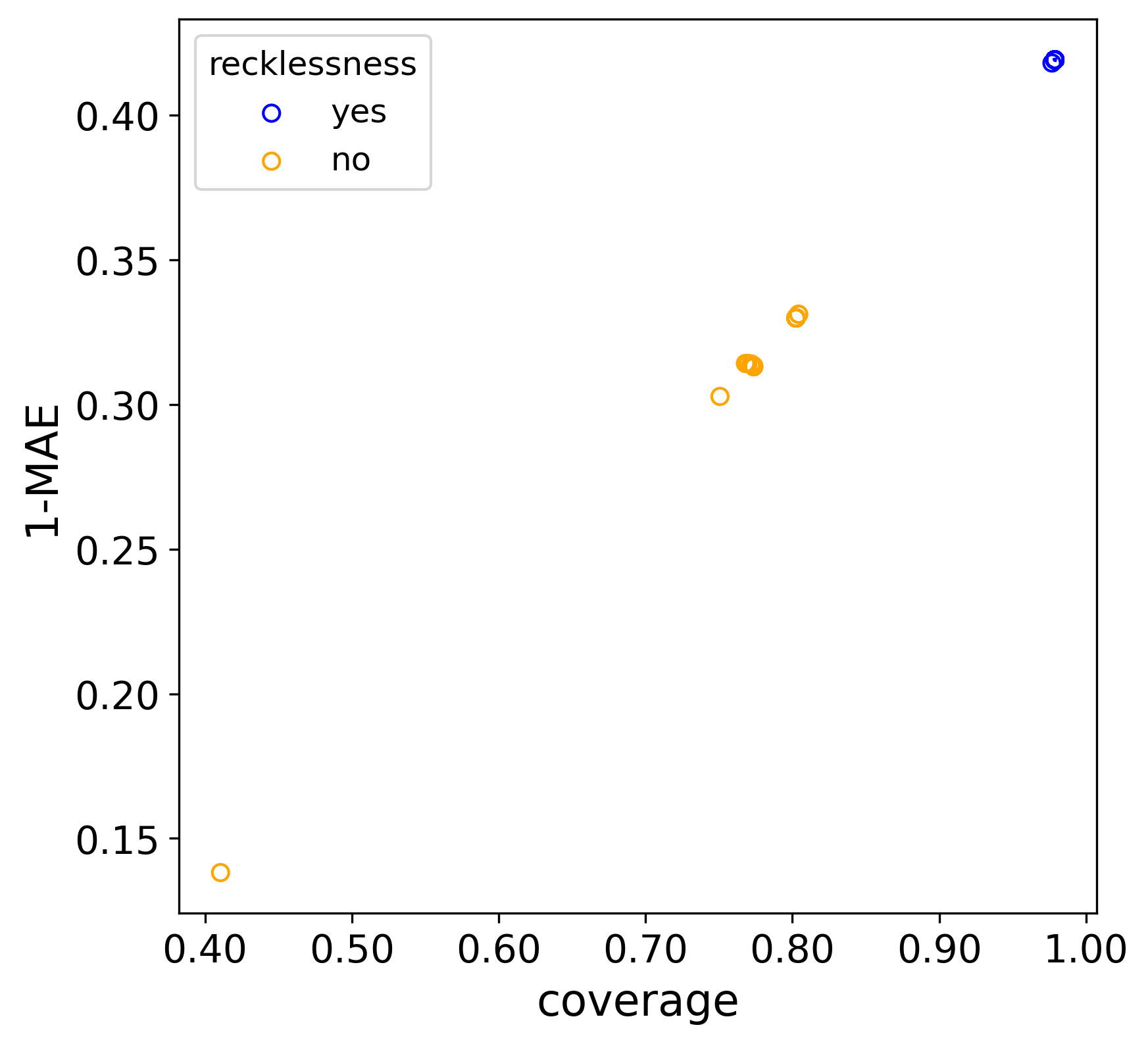
(a) FilmTrust

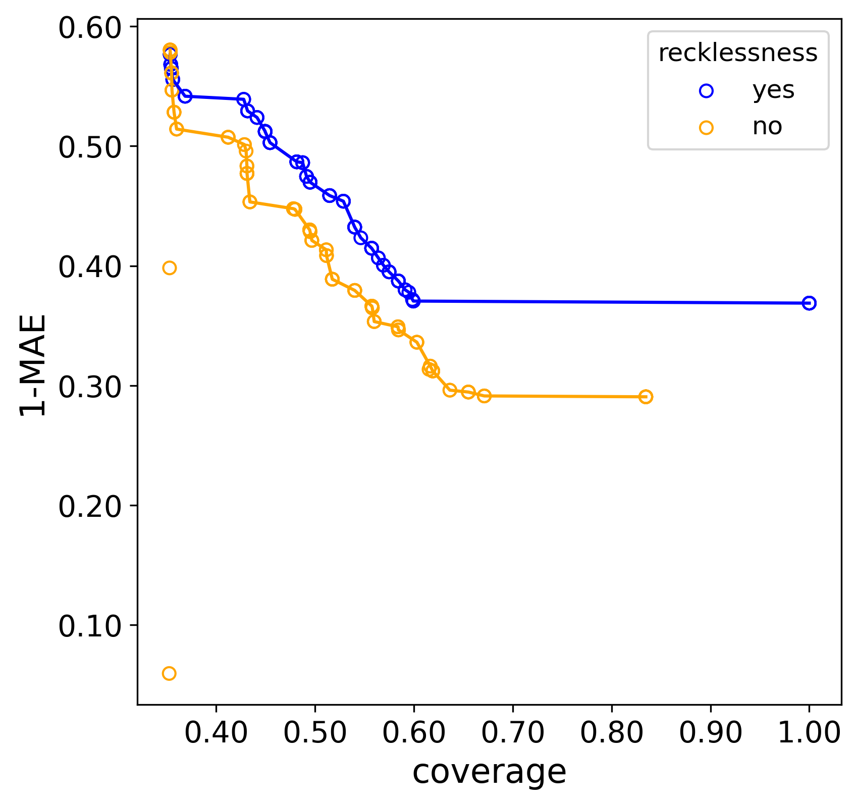
(b) MovieLens100K

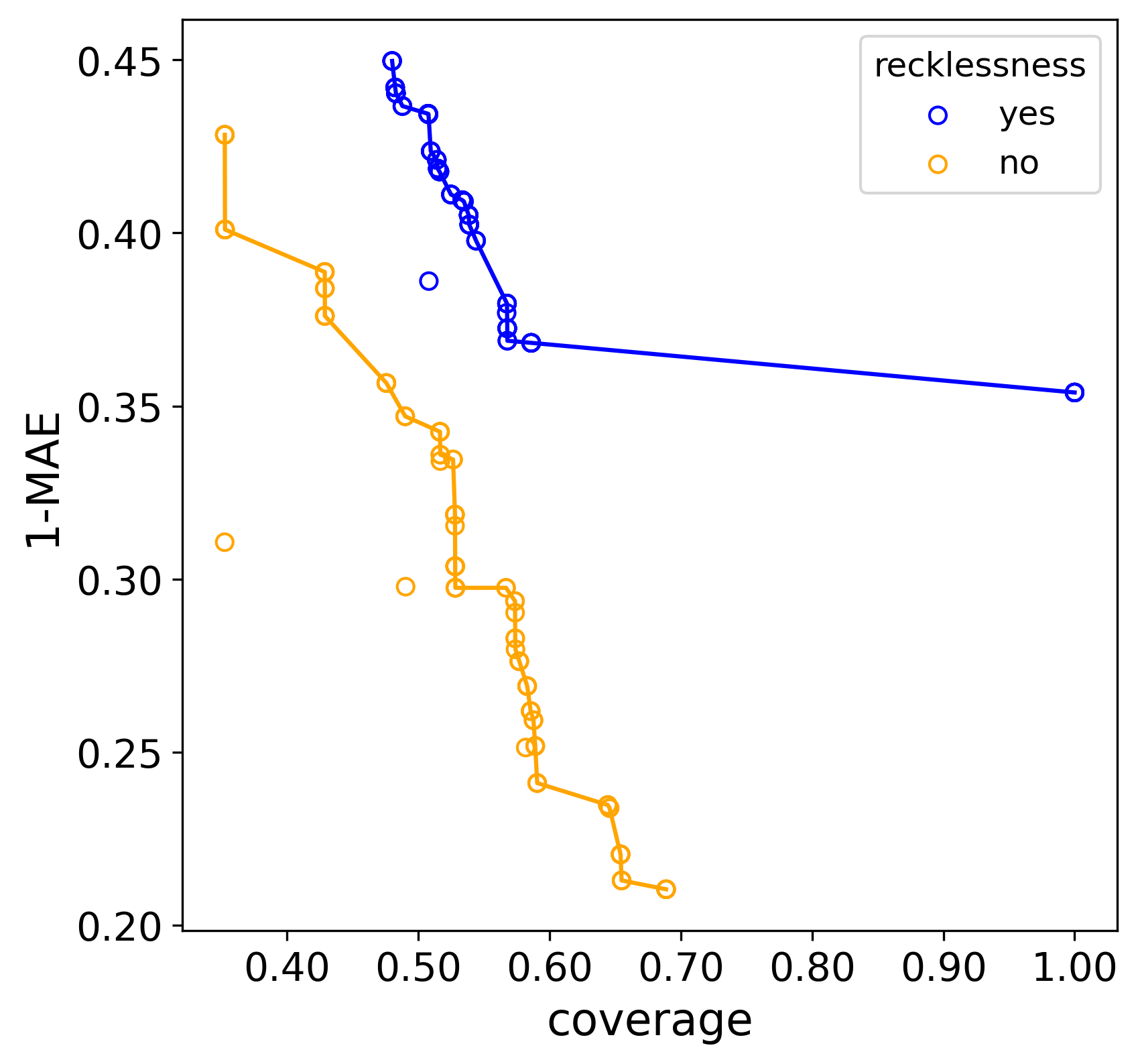
(c) MovieLens1M

Figure 1: Pareto front obtained thorough hyper-parameters optimization using genetic algorithms.

This experiment demonstrates the advantage of using the recklessness regularization. However, it does not show the influence of this regularization on the balance between prediction quality and quantity. Figure 2 displays the value of the recklessness regularization hyper-parameter for all the individuals evaluated by the genetic algorithms. It can be observed that, in general, positive values of recklessness provide a model with many predictions but less accuracy, whereas negative values of recklessness offer a model with fewer predictions but much higher accuracy.

This is consistent with the design of the recklessness regularization (see section 3), as negative values imply that the predicted probability distributions by the model have a smaller variance, are flatter and thus are closer to a uniform distribution. This makes the model more conservative and only provides high reliabilities when it is very certain about the prediction issued. On the contrary, positive values achieve the opposite effect, causing the model to predict spiky probability distributions with high variance and forcing it to issue riskier predictions.

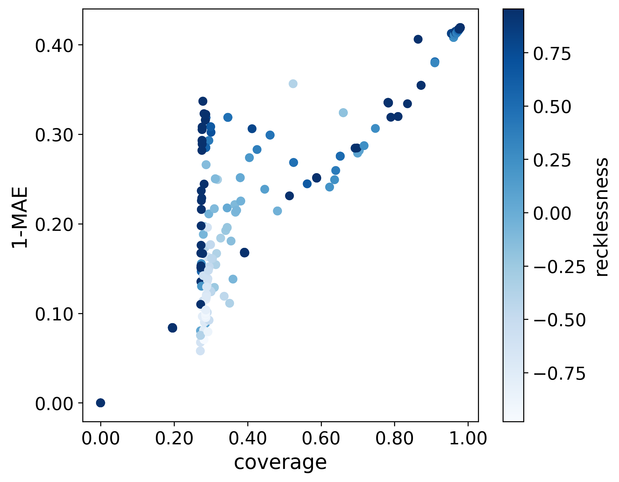
(a) FilmTrust

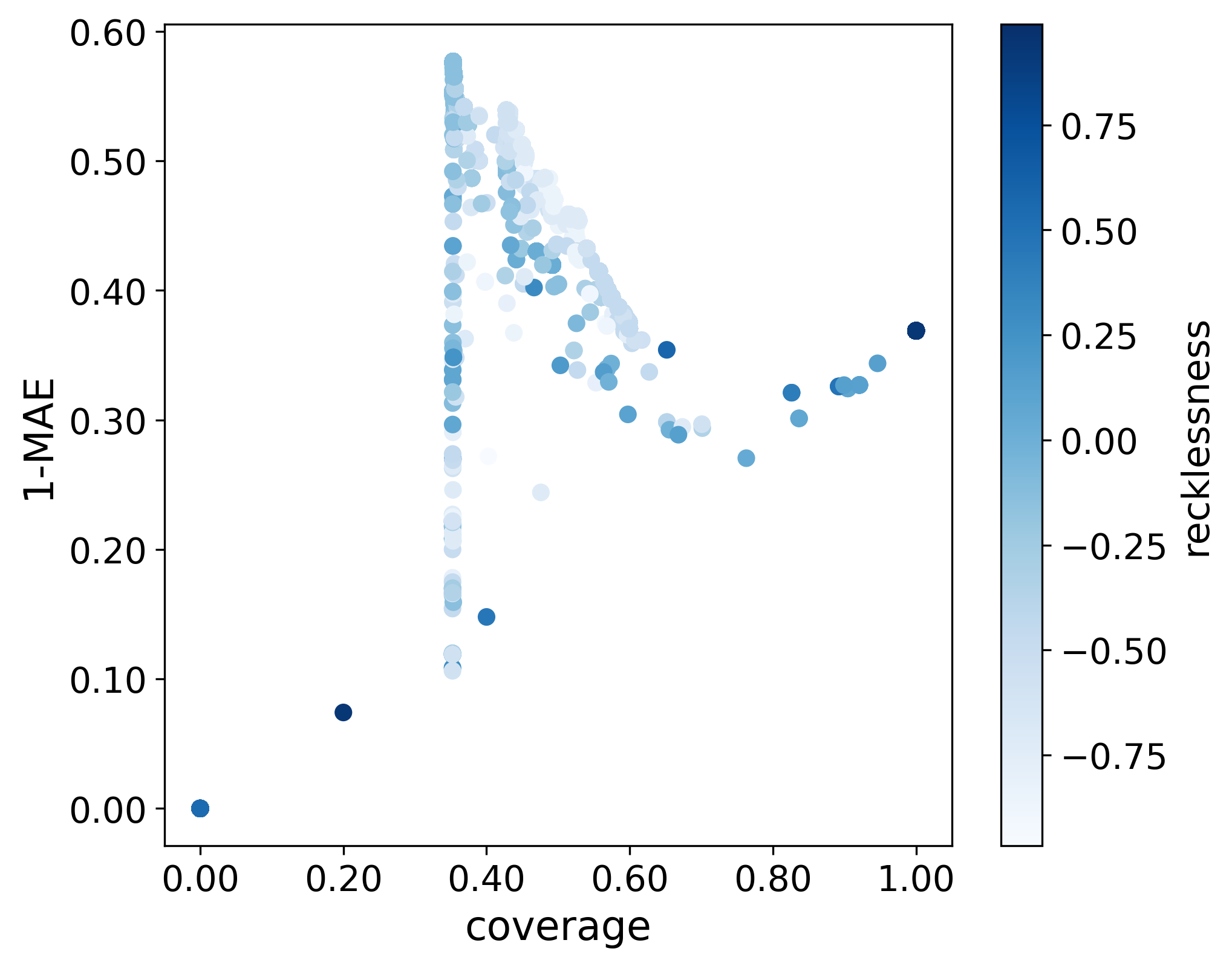
(b) MovieLens100K

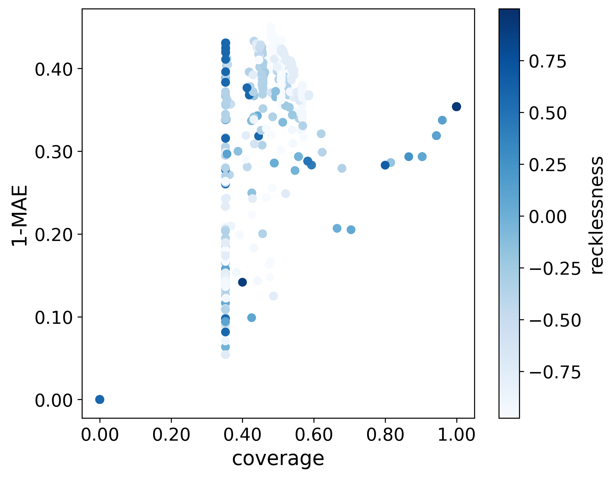
(c) MovieLens1M

Figure 2: Recklessness value of each individual evaluated during the hyper-parameters optimization using genetic algorithms.

These results evidence an improvement in the BeMF model when the recklessness regularization is added. However, all these results have been calculated using validation sets, so overfitting may have occurred in spite of using cross-validation. Figure 3 displays the test results for the Pareto front individuals obtained with the genetic algorithm hyper-parameters optimization. Each dataset is presented in a row of the figure and each column shows the outcome of the quality measures, filtering predictions with a reliability below the threshold indicated on the graph. As in fig. 1, the points represent the results of each individual in the Pareto front, while the lines depict the new Pareto fronts obtained in the test set.

The general trend shown in all the datasets is that as the threshold increases, more accurate predictions are obtained. This is the expected behavior since less reliable predictions should be more erroneous. Additionally, it is observed that solutions with recklessness regularization tend to consistently outperform others in both prediction quality and quantity. In some cases, there is even a single solution that dominates all others. As a result, the Pareto fronts of these results are better when using the recklessness regularization compared to when it is not used.

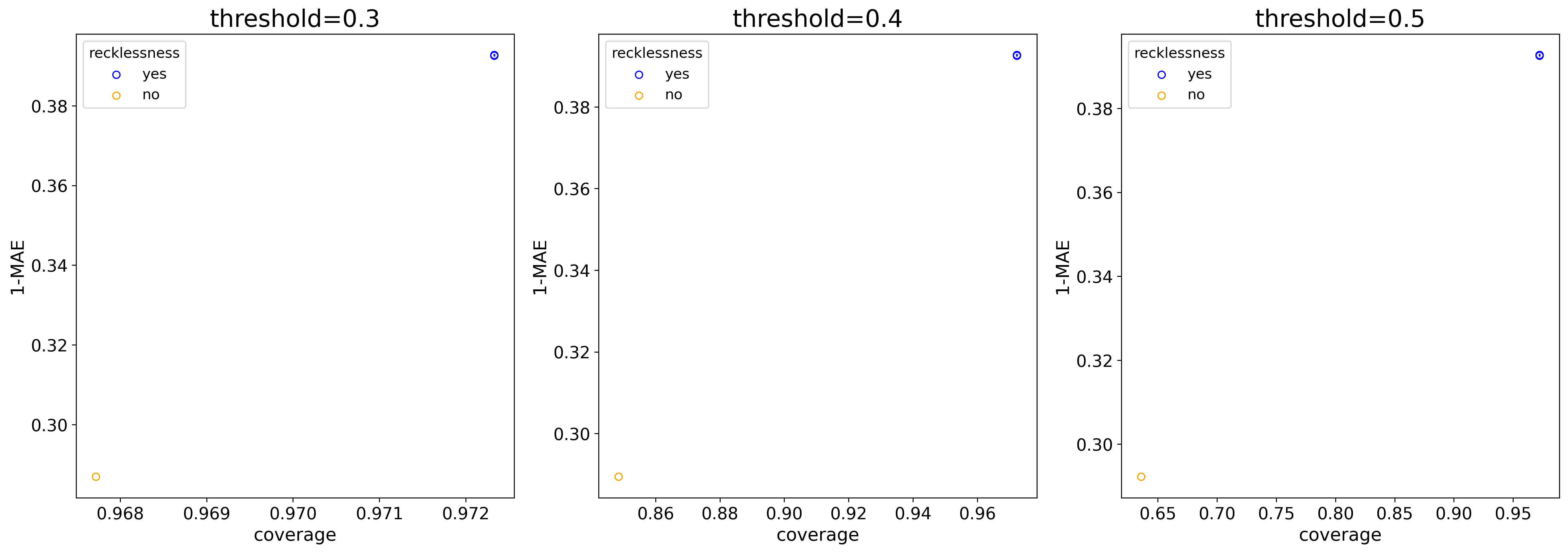
(a) FilmTrust

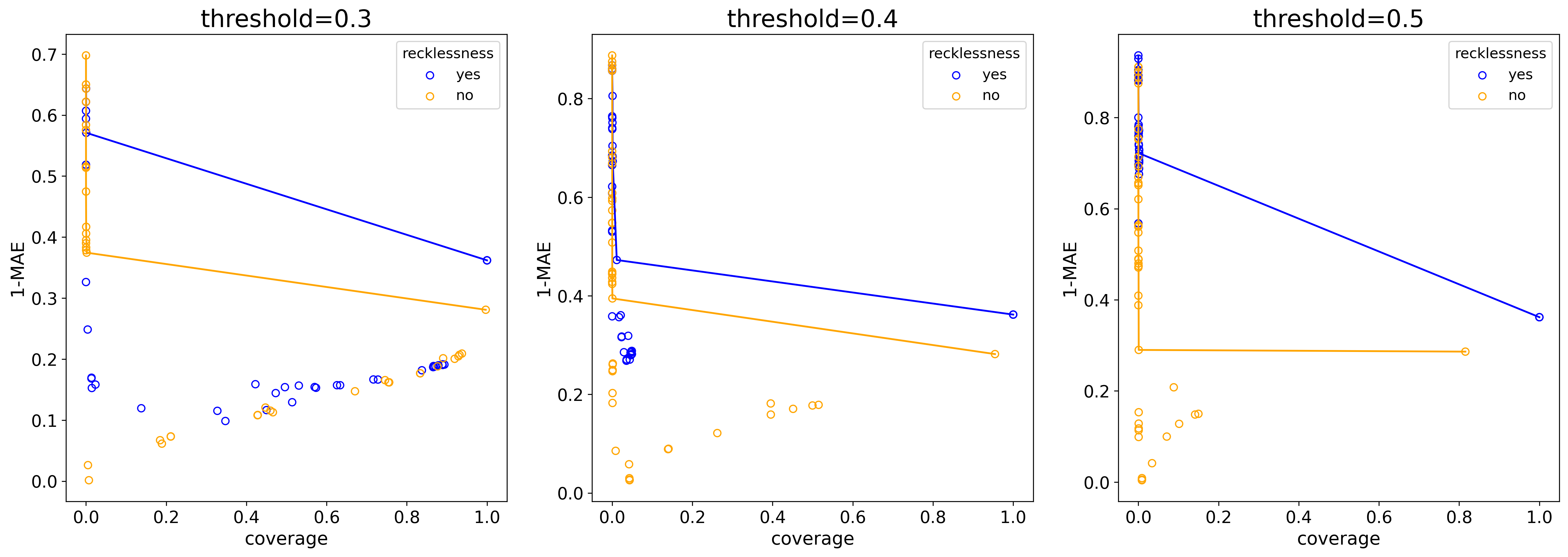
(b) MovieLens100K

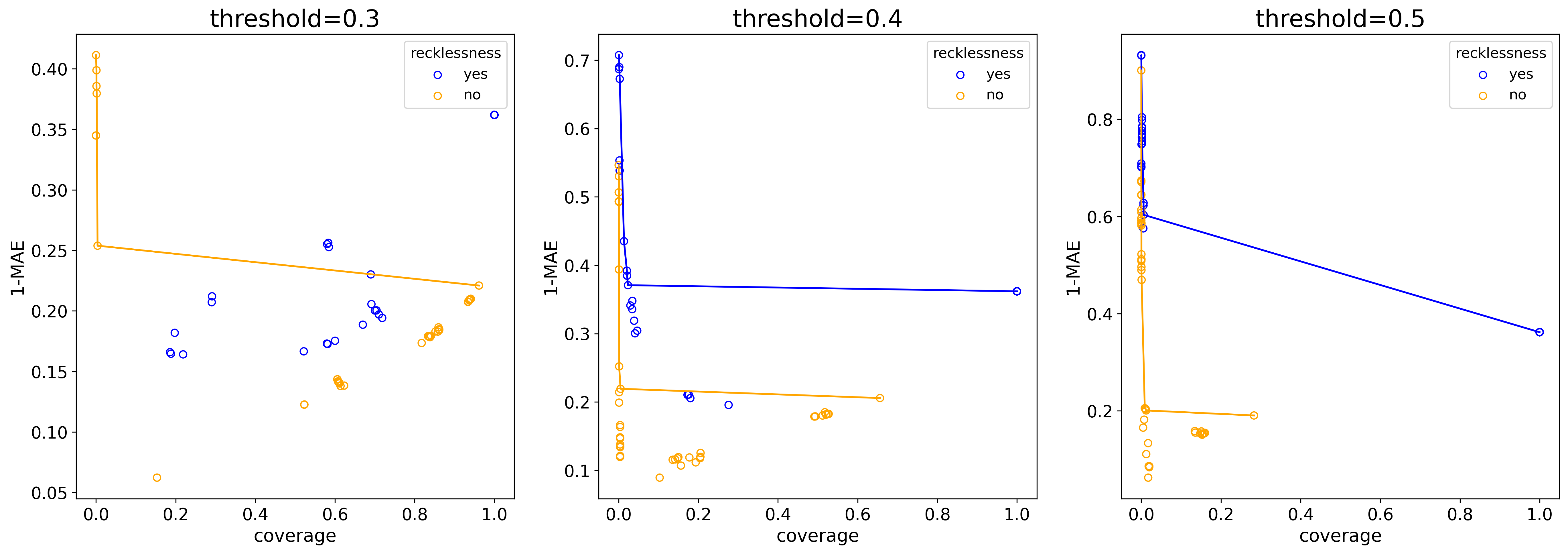
(c) MovieLens1M

Figure 3: Test error of the solutions of the Pareto front found by the genetic algorithm.

As a final analysis, we have compared these Pareto fronts by using their hyper-volume measure, i.e. the volume of the dominated portion of the objective space. This comparison is shown in fig. 4, where the hyper-volume has been calculated both for model with and without recklessness when we filter out predictions with a reliability below the threshold indicated on the horizontal axis of each figure. It can be observed that in FilmTrust, the hyper-volume remains constant and nearly 1 regardless of the threshold value, demonstrating that an almost perfect solution has been found. On the other hand, in MovieLens, the hyper-volume of the model with recklessness is always equal to or greater than the model without recklessness, indicating the advantage of using this new regularization.

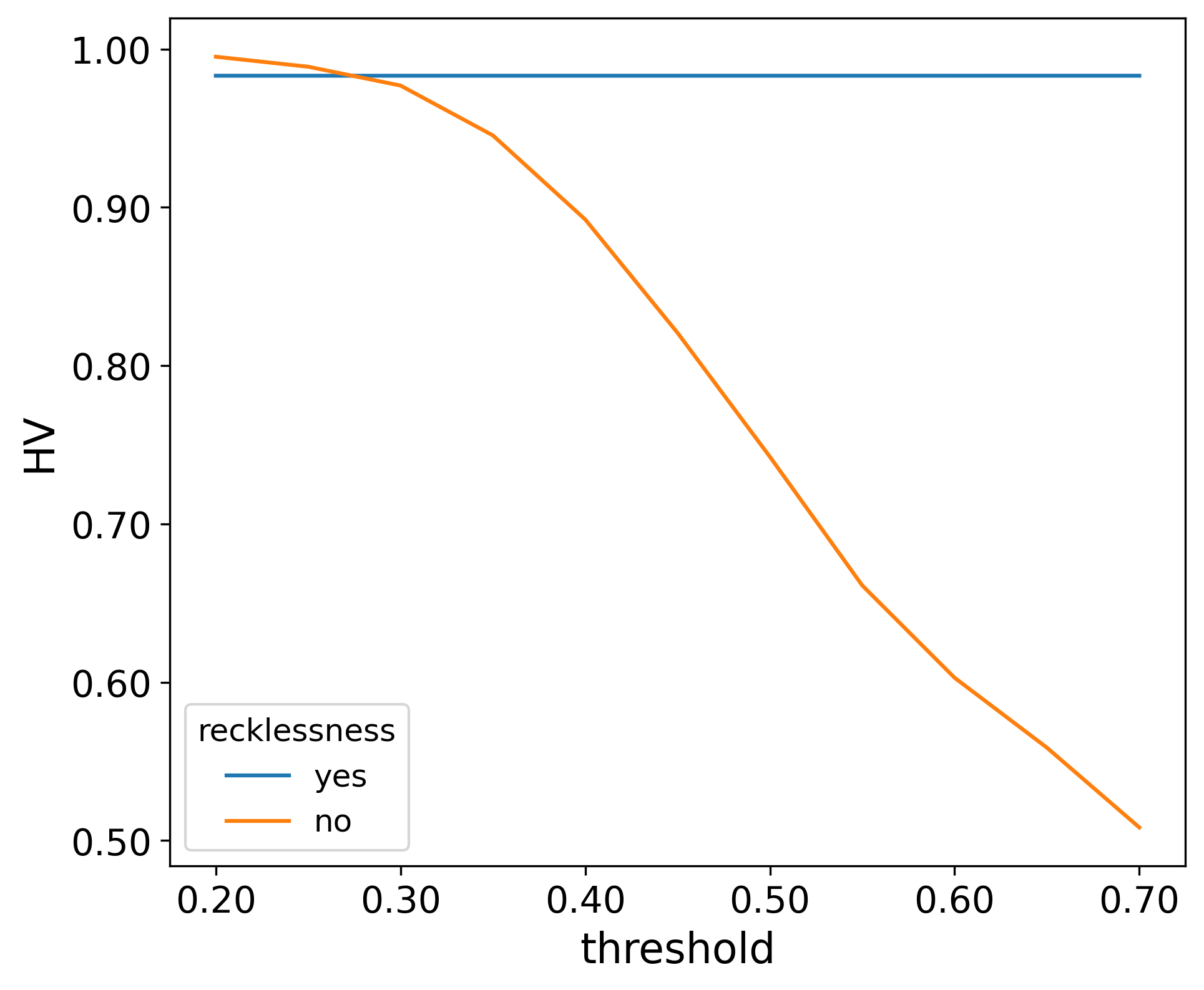
(a) FilmTrust

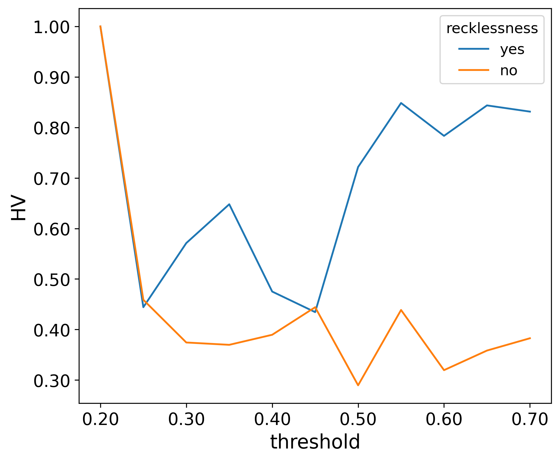
(b) MovieLens100K

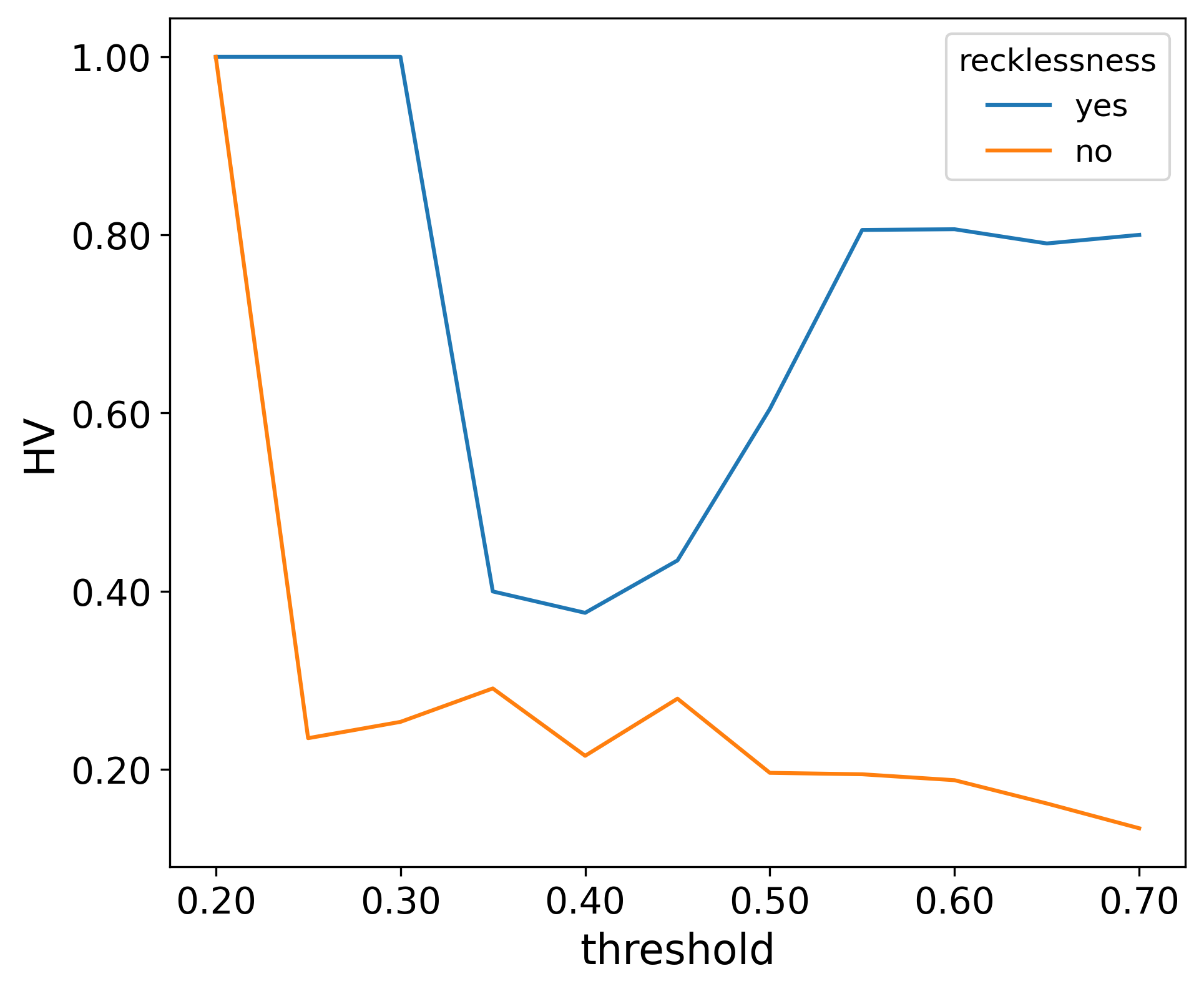
(c) MovieLens1M

Figure 4: Variation of the Pareto front’s hyper-volume in test when filtering all predictions with a reliability lower than the threshold specified.

5 Conclusions and Future Work

In this article, we have introduced a new regularization term for the cost functions of probability-based RS. This new regularization allows us to adjust the variance of the underlying model’s distribution. Negative values of this hyper-parameter results in models with lower variance and providing fewer but highly reliable predictions, while positive values lead to models with higher variance and offering more predictions, though of lower quality. Additionally, this new hyper-parameter improves the RS’s performance in terms of MAE and coverage compared to the same model without the hyper-parameter. All the described results have been validated using three different datasets, and the source code has been provided to ensure reproducibility.

Although the hyper-parameter has only been tested on one RS model, its application in other systems appears promising. Therefore, future work includes evaluating the inclusion of recklessness in other CF systems based on Matrix Factorization (MF). Similarly, applying the concepts of recklessness to CF models based on neural networks [6, 15] or neighborhood-based [33] approaches is also considered.

References

- [1] Sajad Ahmadian, Mohsen Afsharchi, and Majid Meghdadi. A novel approach based on multi-view reliability measures to alleviate data sparsity in recommender systems. Multimedia tools and applications, 78:17763–17798, 2019.
- [2] Sajad Ahmadian, Nima Joorabloo, Mahdi Jalili, and Milad Ahmadian. Alleviating data sparsity problem in time-aware recommender systems using a reliable rating profile enrichment approach. Expert Systems with Applications, 187:115849, 2022.
- [3] Pegah Malekpour Alamdari, Nima Jafari Navimipour, Mehdi Hosseinzadeh, Ali Asghar Safaei, and Aso Darwesh. A systematic study on the recommender systems in the e-commerce. Ieee Access, 8:115694–115716, 2020.
- [4] Santiago Alonso, Jesús Bobadilla, Fernando Ortega, and Ricardo Moya. Robust model-based reliability approach to tackle shilling attacks in collaborative filtering recommender systems. IEEE access, 7:41782–41798, 2019.
- [5] Ricardo Mitollo Bertani, Reinaldo AC Bianchi, and Anna Helena Reali Costa. Combining novelty and popularity on personalised recommendations via user profile learning. Expert Systems with Applications, 146:113149, 2020.
- [6] Jesús Bobadilla, Abraham Gutiérrez, Santiago Alonso, and Ángel González Prieto. Neural collaborative filtering classification model to obtain prediction reliabilities. IJIMAI, 7(4):18–26, 2022.
- [7] Jesús Bobadilla, Fernando Ortega, Antonio Hernando, and Abraham Gutiérrez. Recommender systems survey. Knowledge-based systems, 46:109–132, 2013.
- [8] Germán Cheuque, José Guzmán, and Denis Parra. Recommender systems for online video game platforms: The case of steam. In Companion Proceedings of The 2019 World Wide Web Conference, pages 763–771, 2019.
- [9] Ferdos Fessahaye, Luis Perez, Tiffany Zhan, Raymond Zhang, Calais Fossier, Robyn Markarian, Carter Chiu, Justin Zhan, Laxmi Gewali, and Paul Oh. T-recsys: A novel music recommendation system using deep learning. In 2019 IEEE international conference on consumer electronics (ICCE), pages 1–6. IEEE, 2019.
- [10] Yingqiang Ge, Shuya Zhao, Honglu Zhou, Changhua Pei, Fei Sun, Wenwu Ou, and Yongfeng Zhang. Understanding echo chambers in e-commerce recommender systems. In Proceedings of the 43rd international ACM SIGIR conference on research and development in information retrieval, pages 2261–2270, 2020.
- [11] Ángel González-Prieto, Abraham Gutierrez, Fernando Ortega, and Raúl Lara-Cabrera. Resbemf: Improving prediction coverage of classification based collaborative filtering. arXiv preprint arXiv:2210.10619, 2022.
- [12] G. Guo, J. Zhang, and N. Yorke-Smith. A Novel Bayesian Similarity Measure for Recommender Systems. In Proceedings of the 23rd International Joint Conference on Artificial Intelligence (IJCAI), pages 2619–2625, 2013.
- [13] Pavel Hamet and Johanne Tremblay. Artificial intelligence in medicine. Metabolism, 69:S36–S40, 2017.
- [14] F. Maxwell Harper and Joseph A. Konstan. The movielens datasets: History and context. ACM Transactions on Interactive Intelligent Systems, 5(4):1–19, 2015.
- [15] Xiangnan He, Lizi Liao, Hanwang Zhang, Liqiang Nie, Xia Hu, and Tat-Seng Chua. Neural collaborative filtering. In Proceedings of the 26th international conference on world wide web, pages 173–182, 2017.
- [16] Mengwei Hou, Rong Wei, Tiangang Wang, Yu Cheng, and Buyue Qian. Reliable medical recommendation based on privacy-preserving collaborative filtering. Computers, Materials & Continua, 56(1), 2018.
- [17] Sonoo Thadaney Israni and Abraham Verghese. Humanizing artificial intelligence. Jama, 321(1):29–30, 2019.
- [18] Elvin Isufi, Matteo Pocchiari, and Alan Hanjalic. Accuracy-diversity trade-off in recommender systems via graph convolutions. Information Processing & Management, 58(2):102459, 2021.
- [19] Dietmar Jannach, Ahtsham Manzoor, Wanling Cai, and Li Chen. A survey on conversational recommender systems. ACM Computing Surveys (CSUR), 54(5):1–36, 2021.
- [20] Yehuda Koren, Steffen Rendle, and Robert Bell. Advances in collaborative filtering. Recommender systems handbook, pages 91–142, 2021.
- [21] Yehuda Koren and Joe Sill. Ordrec: an ordinal model for predicting personalized item rating distributions. In Proceedings of the fifth ACM conference on Recommender systems, pages 117–124, 2011.
- [22] Sudhanshu Kumar, Kanjar De, and Partha Pratim Roy. Movie recommendation system using sentiment analysis from microblogging data. IEEE Transactions on Computational Social Systems, 7(4):915–923, 2020.
- [23] Raúl Lara-Cabrera, Álvaro González, Fernando Ortega, and Ángel González-Prieto. Dirichlet matrix factorization: A reliable classification-based recommender system. Applied Sciences, 12(3):1223, 2022.
- [24] Benjamin M Marlin. Modeling user rating profiles for collaborative filtering. Advances in neural information processing systems, 16, 2003.
- [25] Jermaine Marshall and Dong Wang. Mood-sensitive truth discovery for reliable recommendation systems in social sensing. In Proceedings of the 10th ACM conference on recommender systems, pages 167–174, 2016.
- [26] Andriy Mnih and Russ R Salakhutdinov. Probabilistic matrix factorization. Advances in neural information processing systems, 20, 2007.
- [27] Fernando Ortega, Raúl Lara-Cabrera, Ángel González-Prieto, and Jesús Bobadilla. Providing reliability in recommender systems through bernoulli matrix factorization. Information sciences, 553:110–128, 2021.
- [28] Fernando Ortega, Bo Zhu, Jesús Bobadilla, and Antonio Hernando. Cf4j: Collaborative filtering for java. Knowledge-Based Systems, 152:94–99, 2018.
- [29] Lara Quijano-Sánchez, Iván Cantador, María E Cortés-Cediel, and Olga Gil. Recommender systems for smart cities. Information systems, 92:101545, 2020.
- [30] Lionel Robert. The growing problem of humanizing robots. Robert, LP (2017). The Growing Problem of Humanizing Robots, International Robotics & Automation Journal, 3(1), 2017.
- [31] Stuart Russell, Sabine Hauert, Russ Altman, and Manuela Veloso. Ethics of artificial intelligence. Nature, 521(7553):415–416, 2015.
- [32] Scott Schanke, Gordon Burtch, and Gautam Ray. Estimating the impact of “humanizing” customer service chatbots. Information Systems Research, 32(3):736–751, 2021.
- [33] Ramni Harbir Singh, Sargam Maurya, Tanisha Tripathi, Tushar Narula, and Gaurav Srivastav. Movie recommendation system using cosine similarity and knn. International Journal of Engineering and Advanced Technology, 9(5):556–559, 2020.
- [34] Le Wu, Xiangnan He, Xiang Wang, Kun Zhang, and Meng Wang. A survey on accuracy-oriented neural recommendation: From collaborative filtering to information-rich recommendation. IEEE Transactions on Knowledge and Data Engineering, 2022.
- [35] Ting Yuan, Huaigang Wu, Jingjie Zhu, Lingling Shen, and Gang Qian. Ms-ucf: A reliable recommendation method based on mood-sensitivity identification and user credit. In 2018 International Conference on Information Management and Processing (ICIMP), pages 16–20. IEEE, 2018.