Learning Regionalization within a Differentiable High-Resolution Hydrological Model using Accurate Spatial Cost Gradients

Abstract

Estimating spatially distributed hydrological parameters in ungauged catchments poses a challenging regionalization problem and requires imposing spatial constraints given the sparsity of discharge data. A possible approach is to search for a transfer function that quantitatively relates physical descriptors to conceptual model parameters. This paper introduces a Hybrid Data Assimilation and Parameter Regionalization (HDA-PR) approach incorporating learnable regionalization mappings, based on either multivariate regressions or neural networks, into a differentiable hydrological model. It enables the exploitation of heterogeneous datasets across extensive spatio-temporal computational domains within a high-dimensional regionalization context, using accurate adjoint-based gradients. The inverse problem is tackled with a multi-gauge calibration cost function accounting for information from multiple observation sites. HDA-PR was tested on high-resolution, hourly and kilometric regional modeling of two flash-flood-prone areas located in the South of France. In both study areas, the median Nash-Sutcliffe efficiency (NSE) scores ranged from 0.52 to 0.78 at pseudo-ungauged sites over calibration and validation periods. These results highlight a strong regionalization performance of HDA-PR, improving NSE by up to 0.57 compared to the baseline model calibrated with lumped parameters, and achieving a performance comparable to the reference solution obtained with local uniform calibration (median NSE from 0.59 to 0.79). Multiple evaluation metrics based on flood-oriented hydrological signatures are also employed to assess the accuracy and robustness of the approach. The regionalization method is amenable to state-parameter correction from multi-source data over a range of time scales needed for operational data assimilation, and it is adaptable to other differentiable geophysical models.

Irrespective of their type and complexity, hydrological models are more or less empirical and uncertain representations of multiscale coupled hydrological processes whose observability is limited. Hydrological model parameters are in general effective quantities that cannot be directly measured. Instead, they are typically inferred through a calibration procedure aimed primarily at obtaining satisfactory streamflow simulations (e.g., Beven (2001); Kirchner (2006); Gupta et al. (2006); Vrugt et al. (2008)). In most cases, this optimization problem is a difficult ill-posed inverse problem faced with the equifinality (Beven, 2001) of feasible solutions, which can be further interpreted as model structural equifinality and spatial equifinality in the context of spatially sparse observations compared to model controls (see for example discussions in Garambois et al. (2020)). Most calibration approaches enable the estimation of spatially uniform model parameters for a single gauged catchment, but this leads to piecewise constant and discontinuous parameters fields for adjacent catchments. Moreover, parameter sets determined through calibration are not transferable to ungauged locations although the latter represent the majority of the global land surface (Fekete and Vörösmarty, 2007; Hannah et al., 2011). Therefore, prediction in ungauged basins remains a “grand challenge” (Sivapalan, 2003) in hydrology (Hrachowitz et al., 2013), which hinders the development of effective high-resolution models adapted to the simulation of hydrological extremes in a context of high data uncertainty (e.g., for Mediterranean flash floods in Garambois et al. (2015); Jay-Allemand et al. (2022b)).

The estimation of hydrological model parameters in ungauged regions is performed with so-called regionalization approaches that exploit and transfer hydrological information from gauged to ungauged catchments using various descriptors of catchments physical properties (see reviews in Blöschl et al. (2013); Samaniego et al. (2010); Hrachowitz et al. (2013); Beck et al. (2020)). The most widely used approach in early studies for regionalization involved independent catchment-by-catchment calibrations, followed by multiple regression or interpolation techniques to transfer the calibrated parameter sets from gauged to ungauged locations (Abdulla and Lettenmaier, 1997; Seibert, 1999; Parajka et al., 2005; Razavi and Coulibaly, 2013; Parajka et al., 2013) and can be called post-regionalization (Samaniego et al., 2010). This approach presumes that the variability of calibrated model parameters through the catchments have relations based, for instance, on spatial proximity (Widén-Nilsson et al., 2007; Oudin et al., 2008), and physical or climatic similarity (Oudin et al., 2010; Beck et al., 2016). Statistical learning methods have also been applied in post-regionalization to explore the relationships between physical descriptors and calibrated parameter sets at gauged locations (e.g., Saadi et al. (2019); Wang et al. (2023)). However, post-regionalization approaches are limited to lumped parameters, thus ignoring within-catchment variabilities (see reviews in Samaniego et al. (2010); Razavi and Coulibaly (2013)), except when calibrated parameters correspond to tuning factors of physical pedotranfer functions or hydraulic frictions correspondence tables (see Garambois et al. (2015) for details). The identification of transfer functions in post-regionalization is complicated by the uncertainty of estimated parameter sets, while spatial proximity is more adapted to densely gauged river networks and regions (Oudin et al., 2008; Reichl et al., 2009). Moreover, incorporating a statistical learning process, especially unsupervised learning approaches, in the post-regionalization step can exacerbate existing issues such as parameter biases induced by data measurement errors (Kavetski et al., 2006). A regionalized calibration simultaneously exploiting the information of multiple gauges, within spatial clusters defined a priori from descriptors, is performed in Huang et al. (2019) over Norway using climatic similarity. The parameters calibrated over multiple gauges of a climatic zone are applied to ungauged catchments of the same zone. This approach does not account for hydrological heterogeneity within the catchments or within the regional clusters determined by physical similarity, which can have a major impact on the forecasting of extreme floods in particular (Garambois et al., 2015; Jay-Allemand et al., 2022b).

The simultaneous regionalization approach involves optimizing a transfer function between physical descriptors and model parameters (cf. Hundecha and Bárdossy (2004); Götzinger and Bárdossy (2007); Bastola et al. (2008); Samaniego et al. (2010)). In this case and contrarily to post-regionalization, the descriptors-to-parameters mapping is the first optimizable operator of the forward hydrological model. It enables to overcome most of the aforementioned problems and has been applied in several studies. For instance, it has been used for regionalizing semi-distributed models such as: HBV in Hundecha and Bárdossy (2004) or in Götzinger and Bárdossy (2007) who introduced monotonicity and Lipschitz condition into the optimization problem to constrain the inferred spatial fields; TOPMODEL in Bastola et al. (2008) who used an Artificial Neural Network (ANN)-based mapping between catchment descriptors and model parameters (both their value and their uncertainty as quantified by a posterior covariance matrix). A multiscale parameter regionalization (MPR) method, combining descriptors maps, upscalings functions and regionalization transfer functions in the form of multivariate mappings from descriptors, and implemented within a spatially distributed multiscale hydrological model (mHm), has been proposed by Samaniego et al. (2010), and later applied to over 400 European catchments at $0.25^{\circ}$ spatial resolution in Rakovec et al. (2016). This approach imposes a spatial regularization effect that is needed when working with spatially distributed hydrological models and spatially sparse discharge data (see regularization for semi-lumped model calibration from multiple nested gauges in De Lavenne et al. (2019)). The MPR method from Samaniego et al. (2010) has also been used with other gridded hydrological models in large sample applications. For example, Mizukami et al. (2017) calibrate the VIC model at a resolution of $0.125^{\circ}$ over 531 headwater catchments ($\mathrm{area}<2,000\leavevmode\nobreak\ \mathrm{km}^{2}$) in the continguous US area, using a lumped regionalization approach. Another example is Beck et al. (2020), who calibrate the HBV model at $0.05^{\circ}$ resolution over 4,229 headwater catchments ($\mathrm{area}<5,000\leavevmode\nobreak\ \mathrm{km}^{2}$) worldwide. In their study, they categorize the catchments into three climatic groups and perform tenfold cross-validation using $90\%$ of the gauged catchments. While these studies applied MPR deterministically, in Lane et al. (2021), the MPR method is applied within the generalized likelihood uncertainty estimation (GLUE) framework, with a high-resolution HRU model (DECIPHeR framework) at daily time resolution over a large sample of 437 catchments in the UK. However, the routing module in this study is calibrated separately with a simple random sampling approach. In Mizukami et al. (2017), the runoff routing model is a gamma distribution function with two parameters that were “directly calibrated for each basin”. Therefore, those regionalization approaches essentially focus on runoff production, at a daily time step for mostly headwater catchments whose characteristic response/concentration time scale might be shorter. The same remark can be made for Beck et al. (2020) who work at daily time step on headwater catchments, simply without modeling routing.

In all the above studies, state of the art optimization algorithms are used, especially Shuffle Complex Evolution algorithm (SCE) (Duan et al., 1992) in Mizukami et al. (2017), or Distributed Evolutionary Algorithms (DEAP) (Fortin et al., 2012) in Beck et al. (2020), or the GLUE framework with a random sampling approach in Lane et al. (2021). Those algorithms are applicable with low-dimensional controls only, which limits the affordable number of descriptors and the spatialization of regional transfer parameters (that are lumped in all methods above), and more importantly, which limits the affordable complexity of the regionalization operator. Nevertheless, gradient-based algorithms are efficient approaches for solving high dimensional inverse problems, and their potential has been demonstrated in optimization of spatial parameters of hydraulic models (Monnier et al., 2016), or spatially distributed hydrological models (Castaings et al., 2009; Jay-Allemand et al., 2020). They crucially need accurate estimates of cost gradients, i.e. gradients of the cost (objective) function with respect to the sought parameters, which can be spatialized and of large dimension. Such gradients can be computed with an adjoint model for example obtained by source code differentiation in Castaings et al. (2009); Monnier et al. (2016); Jay-Allemand et al. (2020). Note that a key property of neural networks is their differentiability, which makes them compatible with variational data assimilation frameworks (Monnier et al., 2016) and hence suggests them as promising candidate to derive flexible regionalization functions. In the context of hydrological modeling of ungauged basins, achieving such a flexible regionalization is desirable to adequately represent the multi-scale variabilities of the physical system. It would also maximize the extraction of information from large sets of physical descriptors and hydrological response observations, while accounting for data and modeling uncertainties.

A novel approach called HDA-PR (Hybrid Data Assimilation and Parameter Regionalization) is presented in this article. HDA-PR relies on seamless regional optimization algorithms for learning complex transfer functions between physical descriptors and conceptual parameters of spatially distributed hydrological models, applicable at high-resolution with spatial constraints of various rigidity to address the spatial equifinality issue. It is designed to exploit the informative content of massive heterogeneous datasets over large spatio-temporal computational domains, and is therefore adapted to solving high-dimensional inverse problems. Our approach leverages information from multi-site river flow observations and high-resolution data on a 1 $\mathrm{km}^{2}$ and 1 $\mathrm{h}$ resolution grid, relying on the original combination of the following ingredients:

• Learnable regionalization functions via the introduction into the direct hydrological model of an explicit tunable mapping between heterogeneous physical descriptors and spatially distributed unknown conceptual parameters. This mapping allows estimating parameter values while imposing a constraint on their spatial variability, via the use of physical descriptors and a priori knowledge. Multivariate polynomial regressions and neural networks are employed to learn such a complex nonlinear descriptors-parameters mapping.

• A differentiable spatially distributed hydrological model into which the regionalization operators have been implemented. This enables the computation of accurate, spatially-distributed gradients of the calibration cost (objective) function, with respect to the sought regionalization parameters, which can be of high dimension. Obtaining accurate gradients for such high-dimensional parameters is crucially needed for optimization algorithms.

The original combination of the above ingredients amounts to introducing regionalization transfer functions into a variational data assimilation (VDA) algorithm (similar to the tunable differentiable mappings in hydraulic VDA algorithms (Monnier et al., 2016; Garambois et al., 2020)) dedicated to spatially distributed hydrological modeling and high-dimensional inverse problems. This has seldom been investigated especially for regional hydrological learning from multi-site data. The strength of HDA-PR lies in its capability to learn complex relation between physical descriptors and conceptual parameters of spatially distributed models in the context of structural and spatial parametric equifinality. Additionally, our approach aims at ensuring that the hybrid data assimilation algorithm, which integrates an explainable learning process, produces results that can be physically interpreted (see Larnier and Monnier (2020); Höge et al. (2022); Fablet et al. (2021); Althoff et al. (2021)). It is able to enhance calibration scores with deep learning from large heterogeneous datasets while maintaining the interpretability of physics-based hydrological models. The evaluation procedure adopted in this work considers challenging regionalization problems with multi-gauge settings in flash-flood-prone areas and multiple evaluation metrics including flood event hydrological signatures (Huynh et al., 2023). We address the following aspects of the HDA-PR approach: (i) performance at gauged and ungauged sites; (ii) factors determining the performance; and (iii) spatial patterns of the regionalized parameters in relation to information extraction from physical descriptors.

The remaining sections of this paper are organized as follows: Section 1 describes the HDA-PR algorithms and the SMASH spatially distributed hydrological assimilation platform into which they have been implemented. In Section 2, we present the case studies based on two contrasted areas and analyze the performance of HDA-PR using different regionalization mappings. Subsequently, in Section 3, we discuss compelling findings based on the results from the previous section. Finally, in Section 3, we conclude our work and outline potential future research directions.

1 Forward-Inverse Algorithms

This section presents the forward model and inverse algorithms of the proposed HDA-PR method. An algorithm flowchart is provided in Figure 1 to help in global understanding.

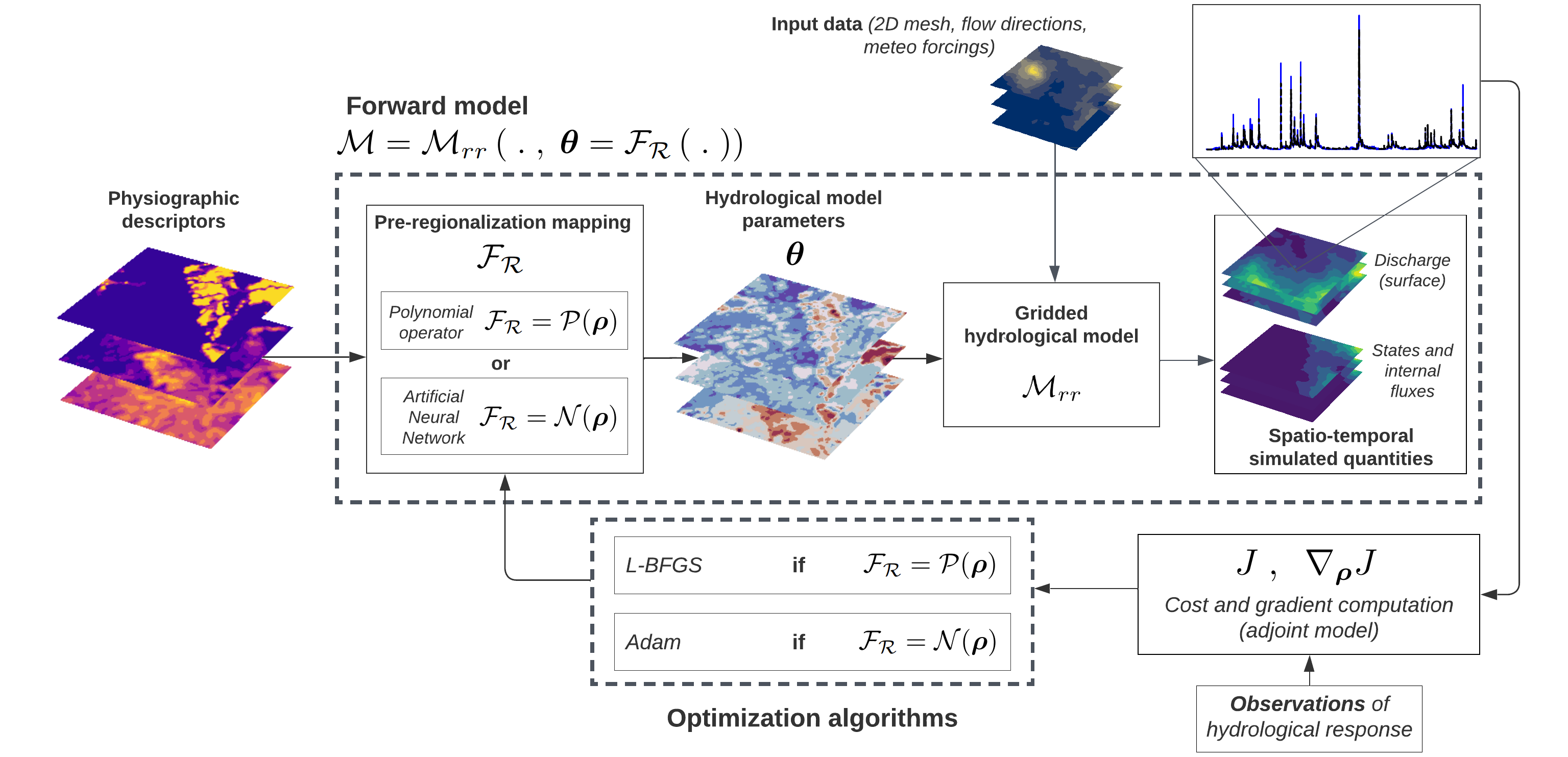
Figure 1: Flowchart of the forward-inverse algorithm used in HDA-PR. The forward hydrological model is a gridded model (spatio-temporal regular grid at 1 $\mathrm{km}^{2}$ and 1 $\mathrm{h}$) using GR operators.

First, the differentiable forward model consists in: (i) a parsimonious and robust GR-like conceptual hydrological model structure (Perrin et al., 2003) that is spatially distributed and differentiable (Jay-Allemand et al., 2020); and (ii) regionalization operators, consisting of either multivariate polynomial regressions or neural networks, for mapping descriptors onto hydrological model parameters. The calibration cost function adapted to multi-site (and potentially multi-source) observations is then defined. The inverse optimization algorithms, that use the spatially distributed gradients of the cost function with respect to model parameters, and are capable of dealing with high-dimensional inverse problems such as encountered with tunable parameters of regionalization descriptors-parameters mappings, are then detailed.

The core strength of HDA-PR is the use of differentiable descriptors-to-parameters transfer functions, especially in the form of neural networks, and the capability to automatically compute accurate cost gradients. The latter enables the use of gradient-based variational optimization algorithms with high-dimensional regional parameter vectors. The method is applicable to any differentiable forward model as well as to multi-source heterogeneous datasets, and hence constitutes a powerful data assimilation framework.

1.1 Forward Model with Regionalization

First, let $\Omega\subset\mathbb{R}^{2}$ denote a 2D spatial domain that can contain multiple catchments, both gauged and ungauged, with a minimum of one gauged catchment, and $t>0$ the physical time. In what follows, the vector of spatial coordinates over $\Omega$ is denoted $x$. The number of active cells within the spatial domain $\Omega$ is noted $N_{x}$. A 2D flow directions map $\mathcal{D}_{\Omega}$ is obtained from terrain elevation processing and will be used for runoff routing, with the only condition that a unique point in the regular mesh $\mathcal{T}_{\Omega}$ has the highest drainage area.

Consider observed discharge time series $Q^{*}_{g}(t)$ at $N_{G}$ observation cells of coordinates $x_{g}\in\Omega$, $g=1..N_{G}$ ($N_{G}\geq 1$). For each observation cell, the corresponding gauged upstream sub-catchment is noted $\Omega_{g}$ so that $\Omega_{ung}=\Omega\setminus\left(\cup_{g=1}^{N_{G}}\Omega_{g}\right)$ is the remaining ungauged part of the whole spatial domain $\Omega$. Note that this definition is suitable for the general regionalization case dealing with spatially independent and/or nested gauged catchments.

Then, the forward model $\mathcal{M}$ can be defined as a multivariate function obtained by partially composing a hydrological model $\mathcal{M}_{rr}$ with a regionalization operator $\mathcal{F}_{R}$ to compute hydrological parameters $\boldsymbol{\theta}$ such that:

$$\mathcal{M}=\mathcal{M}_{rr}\left(\;.\;,\;\boldsymbol{\theta}=\mathcal{F_{R}}\left(\;.\;\right)\right)$$ (1)

Let us now introduce and detail the hydrological model and the regionalization operator along with their input variables.

The rainfall and potential evapotranspiration fields are respectively noted $\boldsymbol{P}\left(x,t\right)$ and $\boldsymbol{E}\left(x,t\right)$, $\forall x\in\Omega$. The hydrological model $\mathcal{M}_{rr}$ is a dynamic operator projecting the input fields $\boldsymbol{P}\left(x,t\right)$ and $\boldsymbol{E}\left(x,t\right)$, given an input drainage plan $\mathcal{D}_{\Omega}\left(x\right)$, onto the discharge field $\boldsymbol{Q}\left(x,t\right)$ and states fields $\boldsymbol{h}\left(x,t\right)$ such that, $\forall(x,t^{\prime})\in\Omega\times\left[0,t\right]$:

$$\boldsymbol{U}\left(x,t\right)=\left(\boldsymbol{h},\boldsymbol{Q}\right)\left(x,t\right)=\mathcal{M}_{rr}\left[(\mathcal{D}_{\Omega},\boldsymbol{\theta})(x);(\boldsymbol{P},\boldsymbol{E})(x,t^{\prime}),\boldsymbol{h}(x,0),t\right]$$ (2)

where $\boldsymbol{\theta}$ is the $N_{\theta}$-dimensional vector of model parameters 2D fields that we aim to estimate regionally with the new algorithms proposed below, and $\boldsymbol{h}$ is the $N_{S}$-dimensional vector of internal model states. In this study, the distributed hydrological model $\mathcal{M}_{rr}$ is a parsimonious GR4-like conceptual structure (Perrin et al., 2003), which is the spatialized “S-GR4” structure presented in Colleoni et al. (2023). The hydrological parameters vector $\forall x\in\Omega$ is:

$$\boldsymbol{\theta}\left(x\right)=\left(c_{p}(x),c_{ft}(x),k_{exc}(x),l_{r}(x)\right)^{T}$$

where the four spatially varying parameter fields are the capacity of the production reservoir ($c_{p}$ in [mm]), the capacity of the transfer reservoir ($c_{ft}$ in [mm]), the parameter ($k_{exc}$ in [mm/dt]) of the non-conservative water exchange flux, and the linear routing parameter ($l_{r}$ in [min]).

In order to constrain and explain these spatial fields of conceptual model parameters $\boldsymbol{\theta}(x)$ from descriptors $\boldsymbol{D}(x)$, we introduce a regionalization operator $\mathcal{F}_{R}$ that is a descriptors-to-parameters mapping such that:

$$\boldsymbol{\theta}\left(x\right)=\mathcal{F}_{R}(\boldsymbol{D}\left(x\right),\boldsymbol{\rho}),\,\forall x\in\Omega$$ (3)

with $\boldsymbol{D}$ the $N_{D}$-dimensional vector of physical descriptor maps covering $\Omega$, and $\boldsymbol{\rho}$ the vector of tunable regionalization parameters that is defined below.

Two types of regionalization operators are used in HDA-PR (see Figure 1):

1. A set $\mathcal{P}$ of multivariate polynomial regression operators for each parameter of the forward hydrological model (Equation 2):

   $$\boldsymbol{\theta}(x,\boldsymbol{D},\boldsymbol{\rho})\coloneqq\mathcal{P}\left(\boldsymbol{D}(x),\boldsymbol{\rho}\right)\equiv\left[\left(\theta_{k}(x,\boldsymbol{D},\boldsymbol{\rho}_{k})\right)_{k=1}^{N_{\theta}}\right]^{T},\,\forall x\in\Omega;$$ (4)

   $$\theta_{k}(x,\boldsymbol{D},\boldsymbol{\rho}_{k})\coloneqq s_{k}\left(\alpha_{k,0}+\sum_{d=1}^{N_{D}}\alpha_{k,d}D_{d}^{\beta_{k,d}}(x)\right),\,\forall k\in[1..N_{\theta}]$$

   with $s_{k}(z)=l_{k}+(u_{k}-l_{k})/\left(1+e^{-z}\right),\,\forall z\in\mathbb{R}$, a transformation based on a Sigmoid function with values in $\left]l_{k},u_{k}\right[$, thus imposing bound constraints in the direct hydrological model such that $l_{k}<\theta_{k}(x)<u_{k},\,\forall x\in\Omega$. The lower and upper bounds $l_{k}$ and $u_{k}$, associated to each parameter field $\theta_{k}$ of the hydrological model (Equation 2) are assumed spatially uniform for simplicity here. The regional control vector to be estimated in this case is:

   $$\boldsymbol{\rho}\equiv\left[\left(\boldsymbol{\rho}_{k}\right)_{k=1}^{N_{\theta}}\right]^{T}\equiv\left[\left(\alpha_{k,0},\left(\alpha_{k,d},\beta_{k,d}\right)_{d=1}^{N_{D}}\right)_{k=1}^{N_{\theta}}\right]^{T}$$ (5)

2. An ANN denoted $\mathcal{N}$, consisting of a multilayer perceptron, aimed at learning the descriptors-to-parameters mapping such that:

   $$\boldsymbol{\theta}(x,\boldsymbol{D},\boldsymbol{\rho})\coloneqq\mathcal{N}\left(\boldsymbol{D}(x),\boldsymbol{W},\boldsymbol{b}\right),\forall x\in\Omega$$ (6)

   where $\boldsymbol{W}$ and $\boldsymbol{b}$ are respectively weights and biases of the neural network composed of $N_{L}$ dense layers. The architecture of the neural network and the forward propagation is detailed in Appendix B and Equation 12. Note that an output layer consisting of a scaling transformation based on the Sigmoid function (cf. Equation 11) enables to impose $l_{k}<\theta_{k}(x)<u_{k},\,\forall x\in\Omega$, i.e., bound constraints on the $k^{th}$-hydrological parameters. The regional control vector in this case is:

   $$\boldsymbol{\rho}\equiv\left[\boldsymbol{W},\boldsymbol{b}\right]^{T}\equiv\left[\left(\boldsymbol{W}_{j},\boldsymbol{b}_{j}\right)_{j=1}^{N_{L}}\right]^{T}$$ (7)

For each regionalization operator (Equation 4 or 6), the regional calibration problem consists in optimizing (in a sense defined below) the regionalization control $\boldsymbol{\rho}$ (Equation 5 or 7) that can be of relatively high dimension since it is proportional to the number of descriptors ($N_{D}$), the number of model parameters ($N_{\theta}$), and the degree of spatialization of the regional controls. Optimization algorithms adapted to the high-dimensional problems of interest, taking advantage of accurate spatially distributed gradients computation with the adjoint of the forward model, are detailed thereafter. Importantly, note that by definition of the mathematical model and given the numerical implementation rules followed, the forward model is differentiable. This is a necessary condition for computing cost gradients with respect to spatially distributed hydrological parameters and obtain those of regional controls, as needed for solving the optimization problem. This is a key idea and property of our proposed algorithms.

The numerical resolution of the ODE (Ordinary Differential Equation)-based operator of the forward hydrological model (Equation 2) relies on an explicit expression of its solution, approximated on the regular mesh $\mathcal{T}_{\Omega}$ of constant step $dx$ with a fixed time step $dt$. All physical descriptors are mapped onto model grid for simplicity here.

Note that adding an upscaling operator after the regionalization scheme (as done in Samaniego et al. (2010)) is feasible in HDA-PR under the condition that it is differentiable (at least numerically), and is a potentially interesting topic for further research, as is improving observation operators. In both cases one could use algebraic expressions or neural networks in the HDA-PR assimilation framework.

1.2 Calibration Cost Function

A calibration cost function is defined to measure the misfit between simulated and observed discharge time series, respectively noted $Q_{g}(t)$ and $Q_{g}^{*}(t)$, for $g\in 1..N_{G}$ gauged cells. In order to measure the discrepancy between observed and simulated quantities from multiple observation sites, we consider the cost function:

$$J=\sum_{g=1}^{N_{G}}w_{g}J_{g}^{*}$$ (8)

with $w_{g}$ a weighting function explained afterwards, $J_{g}^{*}$ a local quadratic metric “at the station”, here $1-NSE$ or $1-KGE_{2}$ (see Appendix A). This cost function is a differentiable and convex function, involving the response of the direct model. It depends on the control vector $\boldsymbol{\rho}$ through the direct model $\mathcal{M}$ (Equation 1) composed of the regionalization operator $\mathcal{F}_{R}$ (Equation 3) and the direct hydrological model $\mathcal{M}_{rr}$ (Equation 2).

The multi-site calibration corresponds to $N_{G}>1$ while $N_{G}=1$ is the classical single-gauge calibration. For $N_{G}>1$, the weighting $w_{g}$ is defined such that $\sum_{g=1}^{N_{G}}w_{g}=1$ and is simply set here as $w_{g}=\frac{1}{N_{G}}$, which represents the average cost over multiple gauges.

1.3 Regional Calibration Algorithms

The inverse problem is written as the following convex optimization problem of the regional control vector $\boldsymbol{\rho}$:

$$\boldsymbol{\hat{\rho}}=\arg\min_{\boldsymbol{\rho}}J\left(\boldsymbol{U}\left(\boldsymbol{\rho}\right)\right)$$ (9)

The regional calibration aims to (i) reduce the misfit between observed and simulated discharges at spatially sparse gauging stations, as evaluated by Equation 8, while (ii) determining hydrological parameter maps $\boldsymbol{\theta}(x)$, relevant for modeling at ungauged sites, thus benefiting from the information extracted from physical descriptors and the spatial constraint induced by the regional transfer functions whose parameters $\boldsymbol{\rho}$ are optimized. The regionalization operator can be expressed as either (i) a multi-polynomial mapping $\mathcal{F}_{R}\equiv\mathcal{P}$ (Equation 4), or (ii) an artificial neural network $\mathcal{F}_{R}\equiv\mathcal{N}$ (Equation 6). In both cases, the regional control vector $\boldsymbol{\rho}$ to optimize is large, and gradient based optimization methods adapted to high-dimensional inverse problems are employed.

1.3.1 Optimization Algorithm for Polynomial Regionalization

In this case, the forward model includes the polynomial descriptors-to-parameters mapping (Equation 4), i.e., $\mathcal{F}_{R}\equiv\mathcal{P}$ and the regional control vector is:

$$\boldsymbol{\rho}\coloneqq\left[\alpha_{k,0},\left(\alpha_{k,d},\beta_{k,d}\right)\right]^{T},\forall(k,d)\in[1..N_{\theta}]\times[1..N_{D}]$$

The optimization problem, represented in Equation 9, is solved using the L-BFGS-B algorithm (limited-memory Broyden–Fletcher–Goldfarb–Shanno bound-constrained) (Zhu et al., 1997). This algorithm is specially adapted to high-dimensional parameter spaces, and in this study, there are no bound constraints on the values of $\alpha_{k,.}$, whereas the exponents $\beta_{k,d}$ are simply sought between 0.5 and 2. This algorithm requires the gradient of the cost function with respect to the sought parameters $\nabla_{\boldsymbol{\rho}}J$. This gradient is computed by solving the adjoint model, which is obtained by automatic differentiation using the Tapenade engine (Hascoet and Pascual, 2013). The entire process is implemented in the SMASH Fortran source code, where the full forward model $\mathcal{M}\equiv\mathcal{M}_{rr}\left(.,\mathcal{P}\left(.\right)\right)$ is a composition of both the hydrological model and the polynomial descriptors-to-parameters mapping.

The background value $\boldsymbol{\rho}^{*}$, used as a starting point for the optimization, is set using a spatially uniform solution $\bar{\boldsymbol{\theta}}^{*}$, which is obtained by a simple global optimization algorithm (Michel, 1989) of the inverse problem (Equation 9) where $\mathcal{M}\equiv\mathcal{M}_{rr}$ and $\boldsymbol{\rho}\coloneqq\overline{\boldsymbol{\theta}}$, as follows:

$$\boldsymbol{\rho}^{*}\equiv\left[\alpha_{k,0}=s^{-1}_{k}\left(\bar{\theta_{k}}^{*}\right),\left(\alpha_{k,d}=0,\beta_{k,d}=1\right)\right]^{T},\forall(k,d)\in[1..N_{\theta}]\times[1..N_{D}]$$

where $s^{-1}_{k}(z)=\ln\left(\frac{z-l_{k}}{u_{k}-z}\right)$ is the inverse Sigmoid.

The termination criterion is determined based on the satisfaction of at least one of the following criteria:

• Maximum number of iterations;

• Cost function criterion: $\frac{J^{(i)}-J^{(i+1)}}{\max\left(\lvert{J^{(i)}}\rvert,\lvert{J^{(i+1)}}\rvert,1\right)}\leq\epsilon\times 10^{6}$ (e.g., $\epsilon\approx 2.22\times 10^{-16}$);

• Gradient criterion: $||\nabla_{\boldsymbol{\rho}}J^{(i)}||_{\infty}\leq 10^{-12}$

where $J^{(i)}$, $||\nabla_{\boldsymbol{\rho}}J^{(i)}||_{\infty}$ are respectively the cost value and its projected gradient at iteration $i$, and $\epsilon$ represents the machine precision.

1.3.2 Optimization Algorithm for Neural Network-based Regionalization

In this case, the forward model includes a descriptors-to-parameters mapping performed with a neural network, i.e., $\mathcal{F}_{R}\equiv\mathcal{N}$ and the regional control vector is $\boldsymbol{\rho}\coloneqq\left[\boldsymbol{W},\boldsymbol{b}\right]^{T}$. The optimization problem (Equation 9) can typically be solved using Adam optimization algorithm (Kingma and Ba, 2014), an efficient stochastic gradient descent algorithm able to adapt the learning rate based upon the first and the approximation of the second moments of the gradients for fast convergence, and only requiring first order gradients of the cost function. In the present case, the cost function writes as:

$$J\left(\boldsymbol{U}\left(\boldsymbol{\rho}\right)\right)=J\big{(}Q^{*},\mathcal{M}_{rr}(.\;,\;\boldsymbol{\theta}=\mathcal{N}(\boldsymbol{D},\boldsymbol{\rho}))\big{)}$$ (10)

This formulation of the cost function highlights its dependency on the forward model $\mathcal{M}\equiv\mathcal{M}_{rr}\left(.,\mathcal{N}\left(.\right)\right)$, which is composed of two components in its numerical implementation: (i) an ANN implemented in Python, which produces the output $\boldsymbol{\theta}$ used as input by (ii) the hydrological model $\mathcal{M}_{rr}$ implemented in Fortran. In order to optimize $J$, its gradients with respect to $\boldsymbol{\rho}$ are required. The main technical difficulty here is to achieve a “seamless flow of gradients” through back-propagation. To overcome this, we divide the gradients into two parts and apply the chain rule with analytical derivation and numerical code differentiation (cf. hybrid VDA course in Monnier (2021) and references therein). First, $\nabla_{\boldsymbol{\theta}}J$ can be computed via the automatic differentiation applied to the Fortran code corresponding to $\mathcal{M}_{rr}$. Then, $\nabla_{\boldsymbol{\rho}}\boldsymbol{\theta}$ is simply obtained by analytical calculus applicable given the explicit architecture of the ANN, consisting of a multilayer perceptron. Finally, the two gradients can be combined as $\nabla_{\boldsymbol{\rho}}J=\nabla_{\boldsymbol{\theta}}J.\nabla_{\boldsymbol{\rho}}\boldsymbol{\theta}$. The termination criterion is determined by a specified number of iterations in the optimization algorithm. A detailed explanation of the network architecture, backward propagation, and the optimization process can be found in Appendix B.

2 Data and Numerical Experiment

2.1 Study Area and Experimental Design

The performance of HDA-PR using various regional optimization algorithms is evaluated based on high-resolution regional modeling of two flash-flood-prone areas located in the South of France (Figure 2). They are characterized by contrasted physical properties and catchments behaviors. The modeling approach is applied to each regional domain that contains multiple gauges downstream of both nested and independent catchments, used together in the optimization process through the multi-site cost function.

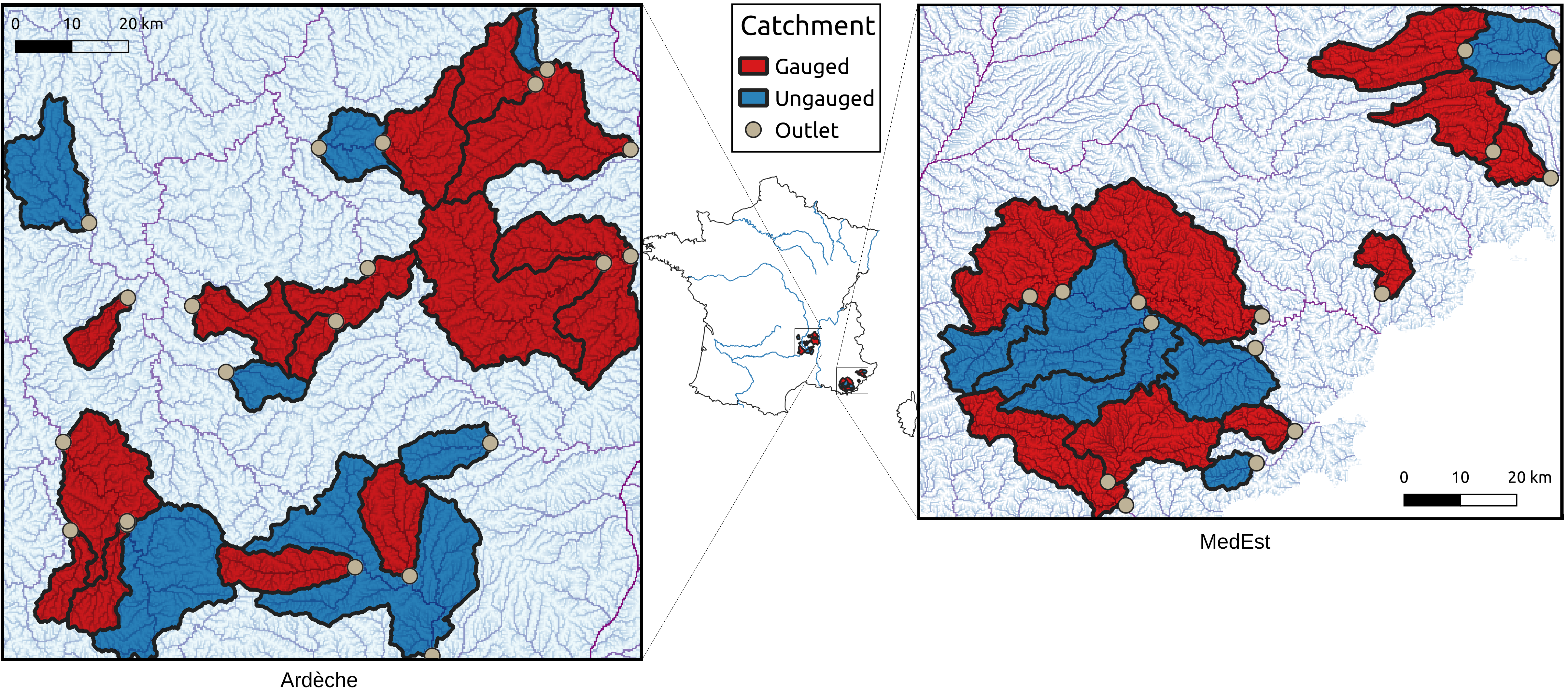
Figure 2: Two study areas on the map on France: Ardèche (left) and MedEst (right). For each area, the gauged catchments (red) are used for multi-site calibration while the pseudo-ungauged catchments (blue) are used for spatial validation.

In order to examine the spatio-temporal extrapolation capabilities of HDA-PR, an a priori partition of the available discharge stations is made into calibration sites and pseudo-ungauged catchments for validation. We selected as gauged stations for regionalization those with good local model performances (i.e., “donor” catchments with potentially lower modeling error). Discharge time series at gauged sites are also split into a calibration and a validation period. A set of 7 physical descriptors (Table 1) available over the whole French territory is used following Odry (2017) and Jay-Allemand et al. (2022b). Note that this setup is sufficient to assess the regionalization performance of the proposed algorithms while keeping the present article concise. The issue of selecting the most relevant information (multi-source observations of hydrological responses and physical descriptors) is intentionally left for future research since it requires several upgrades to the algorithms (dedicated observation operators, descriptors selection layers, etc.). It is worth noting that prior to the optimization process, all descriptors are standardized between 0 and 1 through min-max scaling.

Table 1: Descriptors used as input data for regionalization methods.

Notation	Type	Description	Unit	Source
$d_{1}$	Topography	Slope	∘	Odry (2017)
$d_{2}$	Morphology	Drainage density	-	Organde et al. (2013)
$d_{3}$	Influence	Percentage of basin area in karst zone	%	Caruso et al. (2013)
$d_{4}$	Land use	Forest cover rate	%	CLC European Union (2012)
$d_{5}$	Land use	Urban cover rate	%	CLC European Union (2012)
$d_{6}$	Hydrogeology	Potential available water reserve	mm	Poncelet (2016)
$d_{7}$	Hydrogeology	High storage capacity basin rate	%	Finke et al. (1998)

The first zone is located in the Eastern Mediterranean region and is called “MedEst”. 9 gauged catchments are used for calibration while 6 others are considered as pseudo-ungauged for validation. The second zone is located in the Ardèche region and called “Ardèche”. 14 catchments are considered as gauged while 7 are considered as pseudo-ungauged. Both study areas constitute challenging cases, with contrasted hydrological properties including steep topography and very heterogeneous soils and bedrock (e.g., Garambois et al. (2015)). They are affected by intense rainfall that trigger non linear flash flood responses. Moreover, the MedEst area is the most difficult to model because of the significant proportion of karstic zones. The selection of catchments is based on the availability of long time series with high quality of observed flow and limited anthropogenic impacts. The SMASH model is run on a $dx=1\leavevmode\nobreak\ \mathrm{km}$ spatial grid at $dt=1\leavevmode\nobreak\ \mathrm{h}$ time step. It is forced by: (i) observed rainfall grids based on hourly ANTILOPE J+1 radar-gauge rainfall reanalysis from Météo-France (Champeaux et al., 2009); (ii) potential evapotranspiration (PET) estimated using the formula of Oudin et al. (2005); and (iii) temperature data from SAFRAN reanalysis produced by Météo-France on a 8x8 $\mathrm{km}^{2}$ spatial grid (Quintana-Seguí et al., 2008) downscaled to a 1x1 $\mathrm{km}^{2}$ spatial grid.

For each study area, we perform multi-site regional calibration methods using gauged catchments. The chosen calibration metric is the NSE, computed using data from multiple gauges over a ten-year period (2006-2016). The following calibration methods are compared:

• Local calibrations for each gauge, both with spatially uniform (i.e., $\boldsymbol{\rho}\equiv\bar{\boldsymbol{\theta}}$) and full spatially distributed controls (i.e., $\boldsymbol{\rho}\equiv\boldsymbol{\theta}\left(x\right)$), that are respectively under and over parameterized hydrological optimization problems. These represent reference performances, denoted “Uniform (local)” and “Distributed (local)”.

And multi-gauge regional calibrations with:

• lumped model parameters (i.e., $\boldsymbol{\rho}\equiv\bar{\boldsymbol{\theta}}$) which somehow represents “level 0” regionalization, denoted “Uniform (regionalization)”;

• a multivariate linear mapping (i.e., $\boldsymbol{\rho}\equiv\left[\alpha_{k,0},(\alpha_{k,d},1)\right]^{T}$), denoted “Multi-linear (regionalization)”;

• a multivariate polynomial mapping (i.e., $\boldsymbol{\rho}\equiv\left[\alpha_{k,0},(\alpha_{k,d},\beta_{k,d})\right]^{T}$), denoted “Multi-polynomial (regionalization)”;

• a multilayer perceptron (i.e., $\boldsymbol{\rho}\equiv\left[\boldsymbol{W},\boldsymbol{b}\right]^{T}$), denoted “ANN (regionalization)”.

To ensure robust validation, model performances are assessed in terms of spatial validation, temporal validation, and spatio-temporal validation, with a validation period covering two years from 2016 to 2018. Various evaluation metrics are also used, including multiple hydrological signatures-based metrics from Huynh et al. (2023).

2.2 Regional Learning Performance

In this section, the regional learning performance is analyzed with primary focus on the MedEst region, which represents the most challenging study area. First, Figure 3 suggests that using lumped model parameters $\bar{\boldsymbol{\theta}}$ leads to a poor performance in simulating discharges, whereas the other three regional learning methods result in similar signals with remarkably improved performance, in both the gauged and the pseudo-ungauged catchments.

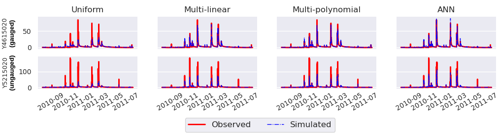
Figure 3: Study area: MedEst. One year of observed and simulated discharges (in $m^{3}/s$) obtained with four multi-gauge regional calibration methods at one gauged (Y4615020) and one pseudo-ungauged catchment (Y5215020).

Given the complexity and heterogeneity of the region, it is unsurprising that lumped model parameters regionalization is unable to accurately reproduce contrasted hydrological responses. Figure 4 demonstrates that the three regionalization methods incorporating information from physical descriptors lead to largely superior performance when compared to the Uniform baseline for the calibration catchments. For example, the NSE scores increase from 0.3 to more than 0.7 in catchment Y5615030, or from 0.4 to more than 0.75 in catchment Y5615010. In addition, these three methods yield relatively high scores in the pseudo-ungauged catchments used for spatial validation (e.g., in Y5215020 where the NSE score has been improved from 0.36 up to 0.83 in the case of ANN). Note that some stations have many missing data: for instance, 32 % of the data are missing for catchment Y5106610, and 21 % for catchment Y5005210. This may affect the NSE scores and at least partly explain the poor validation performances for all methods.

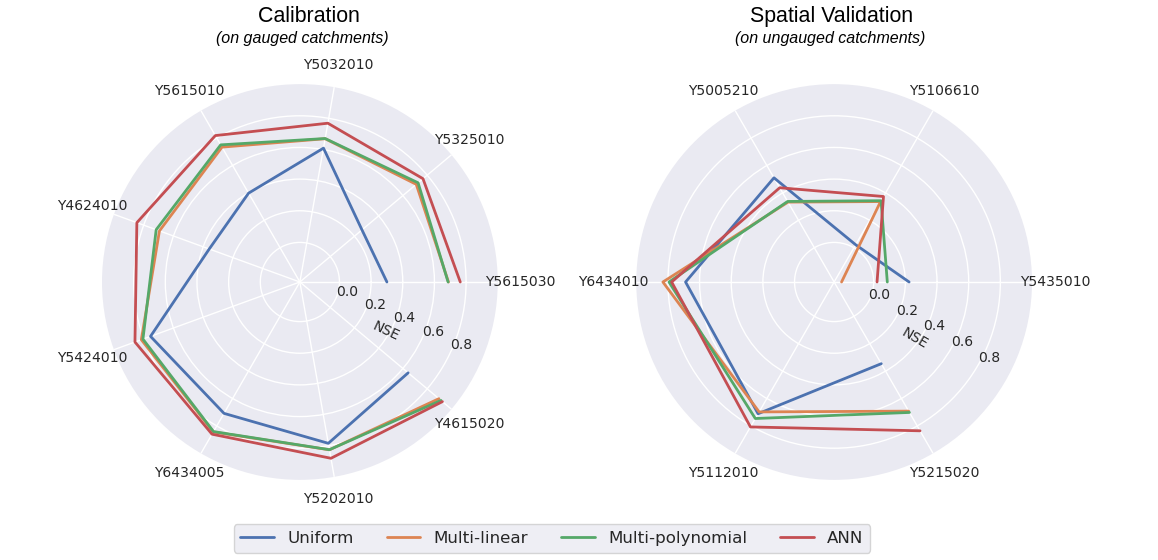
Figure 4: Study area: MedEst. Radial plots of the NSE (optimal value = 1) in gauged catchments (left) and pseudo-ungauged catchments (right) during the calibration period for four multi-gauge regional calibration methods.

We now focus on the global results in both study areas, Ardèche and MedEst, as presented in Figure 5. This figure summarizes the NSE scores for the two local calibration methods (spatially uniform and spatially distributed calibrations) and the four regionalization methods. A rapid interpretation reveals that in the Ardèche area, making the model parameters vary in space seems unnecessary, given the already good performance of the lumped parameters (Uniform) methods in the context of a less complex area. However, it is worth noting that the three regionalization methods also achieve satisfying results, with the median efficiencies (NSE) exceeding 0.65 in both gauged and pseudo-ungauged catchments during the validation period. This suggests that while not necessary, using a non-uniform regionalization approach does not deteriorate the performance in spatial or temporal validation. In contrast and as evidenced in the preceding figures, significant disparities in efficiency scores are observed among the regionalization methods in the MedEst area, where the multivariate regressions and ANN outperform the uniform regionalization baseline calibrated with lumped model parameters. The three methods demonstrate promising results, achieving median NSE scores above 0.72, 0.51, 0.76 and 0.61 (compared to 0.6, 0.41, 0.2 and 0.16 for the baseline) respectively, across calibration, spatial validation, temporal validation and spatio-temporal validation. Specifically, when considering temporal validation, the ANN reaches a median NSE score of approximately 0.9 with eight out of nine stations exceeding a score of 0.8, which is comparable to the performance of the local calibration reference with spatially distributed controls.

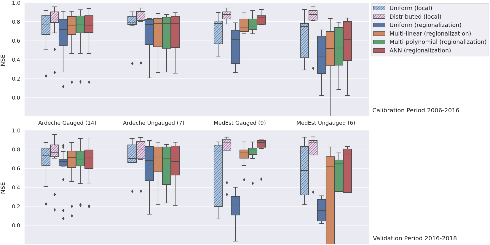
Figure 5: Comparison of NSE scores across gauged and pseudo-ungauged catchments during the calibration (top) and validation (bottom) periods for two local calibration methods and four regionalization methods in both study areas. The numbers in parentheses indicate the number of catchments included in each boxplot.

In order to obtain a more robust evaluation criterion adapted to flood modeling, we consider validation in terms of multiple evaluation metrics based on hydrological signatures for flood events, which are computed via an automated segmentation algorithm proposed by Huynh et al. (2023). Turning the focus back to MedEst, the three non-uniform regionalization methods, with a particular focus on the ANN, demonstrate their ability to outperform the uniform regionalization (lumped model parameters), in both temporal and spatio-temporal validation, as shown in Figure 6. The relative errors (median over flood events) of simulated signatures using these three regionalization methods are around 0.2 compared to more than 0.8 for the uniform baseline in temporal validation, and between 0.2 and 0.6 compared to more than 0.7 for the baseline in spatio-temporal validation. Especially, in the case of ANN, the error in simulating the peak flow is drastically reduced from 0.85 and 0.91 (for the baseline) to 0.28 and 0.43, respectively, in temporal and spatio-temporal validation. It is noteworthy that these flood signatures-based metrics were not included in the cost function during the calibration process, which further supports the robustness and power of the regionalization methods, particularly the one based on the ANN. It thus underscores the potential of such approaches for enhancing flash flood forecasting system.

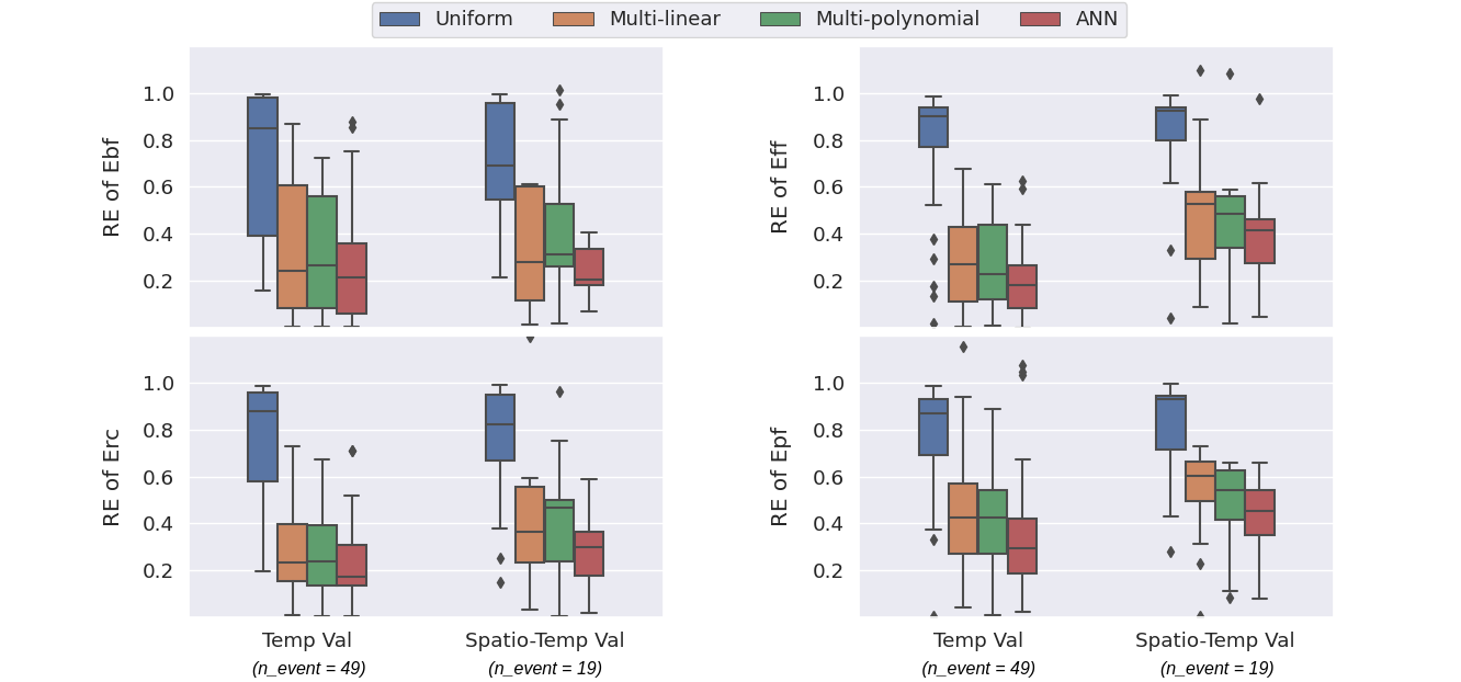
Figure 6: Study area: MedEst. Relative error (RE, optimal value = 0) of 4 flood event signatures: base flow (Ebf), flood flow (Eff), runoff coefficient (Erc) and peak flow (Epf), evaluated using $n\_event=49$ flood events at gauged catchments for temporal validation (Temp Val) and $n\_event=19$ flood events at pseudo-ungauged catchments for spatio-temporal validation (Spatio-Temp Val).

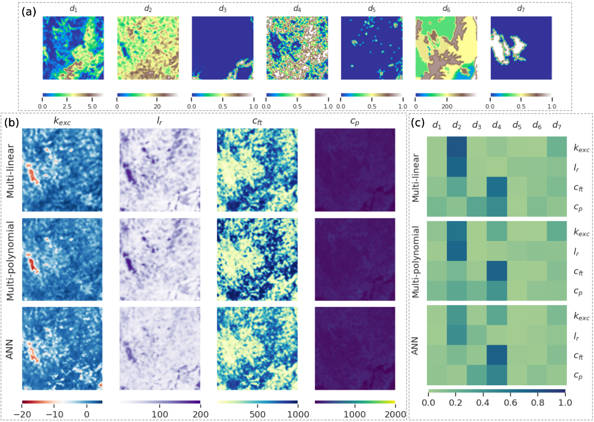
Figure 13: Study area: Ardèche. Sub-figure a: Maps of input descriptors ($d_{1}$-$d_{7}$), whose information is provided in Table 1. Sub-figure b: Calibrated hydrological parameters $(k_{exc},l_{r},c_{ft},c_{p})$ maps for three non-uniform regionalization methods. Sub-figure c: Linear correlation between descriptor and parameter for the three regionalization methods.

Finally, Figure 7-b shows the parameter maps obtained with the three non-uniform regionalization methods, that can be physically interpreted. In general, the spatial patterns of the drainage density ($d_{2}$) in Figure 7-a are easily observable in the distributed parameter maps in the two regression cases, as evidenced by strong correlations between this descriptor and the four model parameters. Such correlations can be quantified using one-to-one parameter-descriptor correlation matrices (Figure 7-c). The relations between the model parameters and physical descriptors are not limited to linear and polynomial forms in the ANN case, leading to parameter maps that are quite distinct from the regression-based ones. Furthermore, it is noteworthy that the ANN can identify stronger correlations (compared to both regression cases) for the routing parameter ($l_{r}$) and the transfer parameter ($c_{ft}$) with the karst index ($d_{3}$). For Ardèche, parameter maps show a reduced variability (see Figure 13-b), and the ANN identifies maps and relations between descriptors and parameters which are similar to those found in both regression cases (see Figure 13-c). This finding suggests that the ANN can effectively approximate the multi-linear regression when dealing with areas like Ardèche, where it does not necessitate more intricate mappings. This demonstrates the robustness and flexibility of the ANN, which proves to be efficient not only in complex study areas but also in simpler ones.

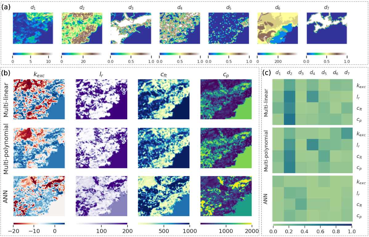
Figure 7: Study area: MedEst. Sub-figure a: Maps of input descriptors ($d_{1}$-$d_{7}$), whose information is provided in Table 1. Sub-figure b: Calibrated hydrological parameters $(k_{exc},l_{r},c_{ft},c_{p})$ maps for three non-uniform regionalization methods. Sub-figure c: Linear correlation between descriptor and parameter for the three regionalization methods.

The corresponding figures in this section depicting the results in Ardèche can be found in Appendix C. The following section focuses on results more specific to the optimization process and provide insights on the use of multivariate regressions and ANN in both study areas.

3 Discussions

Learning the spatial variability of conceptual hydrological parameters may be difficult to achieve with simple regionalization methods (e.g., based on multi-linear regression). However, while complex regional mappings can reduce the misfit between observed and simulated hydrological responses, their ability to produce physically interpretable results may be questioned. This section presents compelling findings and insightful observations obtained from the calibration using HDA-PR, with a particular focus on the learning process in the case of ANN.

When calibrating a model with gradient-based optimization algorithms, it is important to discuss the descent of the cost function. This analysis enables understanding how optimization algorithms converge towards the global or local minimum of the cost function, and identifying potential trade-offs between model flexibility and overparameterization, in addition to validation results. Similar results are observed in both study areas, including the descent of the cost function $J$ and its projected gradient $\nabla_{\boldsymbol{\rho}}J$, which are represented in Figure 8 for the MedEst area.

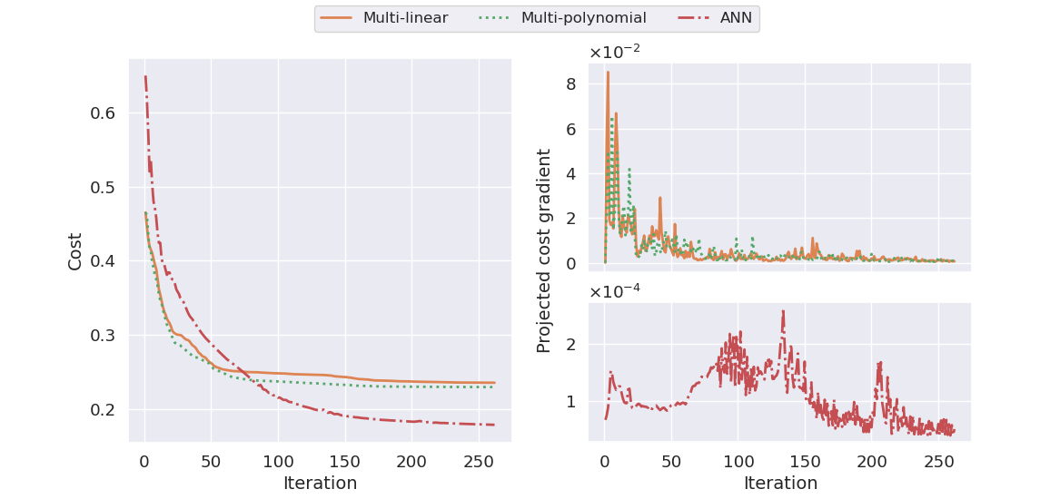
Figure 8: Study area: MedEst. The descent of the cost $J=1-NSE$ (left) and projected gradient $||\nabla_{\boldsymbol{\rho}}J||_{\infty}$ (right) for the three non-uniform regionalization methods.

It is apparent that the cost functions in the two regression methods start from a more optimal point (approximately 0.46) than the ANN since they use a uniform background solution obtained by a global optimization method, as mentioned in 1.3.1. Furthermore, they converge after around 200 iterations and remain monotonous throughout the optimization process. The polynomial regression approach achieves a slightly lower cost than the linear approach, due to the fact that it has nearly twice the number of parameters (Table 2), while the ANN, with a significantly larger number of parameters, can achieve a lower cost despite starting from a higher cost. Moreover, the ANN cost function in the left panel of Figure 8 is not monotonous throughout iterations: it shows localized increases for several instances within the first 100 iterations.

Table 2: Number of parameters in the control vector for the four regionalization methods studied, where $N_{\theta}=4$ and $N_{D}=7$. A detailed calculation of the total number of parameters for the ANN is provided in Table 3. The last two columns show the ratios between the number of parameters in the four methods studied and the fully distributed calibration method (i.e., $\boldsymbol{\rho}\equiv\boldsymbol{\theta}(x)$), which was overparameterized and unable to perform regionalization.

Mapping	Coefficient	Exponent	Total parameters	% (MedEst)	% (Ardèche)
Uniform	$N_{\theta}.1=4$	$0$	$4$	$0.03$	$0.04$
Multi-linear	$N_{\theta}(N_{D}+1)=32$	$0$	$32$	$0.21$	$0.29$
Multi-polynomial	$N_{\theta}(N_{D}+1)=32$	$N_{\theta}.N_{D}=28$	$60$	$0.39$	$0.54$
ANN			$6276$	$40.3$	$56.48$
Fully distributed: $N_{\theta}.N_{x}$. Remind that $N_{x}$ is the number of active cells within the spatial domain $\Omega$.

The variability of the projected cost gradient shown in the right panels of Figure 8 suggests that the surface of the cost function is more complex for ANN than for the two regressions. This is confirmed by the gradient values in the right panels of Figure 8: multi-linear regression lead to projected gradients that are marginally higher than those of multi-polynomial regression but much higher than those of ANN. This discrepancy can be attributed to the complexity of the regionalization mapping in each case, with the ANN being the most complex. Moreover, jumps in the projected gradient (bottom right panel) suggest that the solutions of the ANN can explore different paths and avoid getting stuck in local minima: there are four instances (around iterations 5, 90, 130, and 210) where significant changes occur in the control vector space (biases and weights) to locate the optimum. This property could be essential in tackling equifinality and reach robust global optimum even with different starting points.

To alleviate the vanishing gradient problem inherent in the ANN, we employed several techniques commonly used in the machine learning community. First, we applied Xavier initialization (Glorot and Bengio, 2010) to the weights, maintaining a reasonable magnitude of the gradients. Second, we utilized the ReLU activation function or its variants in the hidden layers, enabling the gradient to flow more freely through the network. Third, we varied the number of hidden layers between 2 and 4, striking a balance between network flexibility and exacerbation of the vanishing gradient problem. Ultimately, we employed a relatively high initial learning rate (e.g., 0.005) to prevent the gradients from shrinking excessively during training.

One can also inquire about the way the different regionalization mappings transfer information from physical descriptors to hydrological parameters. For instance, how can we ensure that HDA-PR effectively uses the physical patterns provided by descriptor maps to constrain the estimation of meaningful spatial parameter maps? To address this question, it is worth noting that the “safest” approach is to use multi-linear regression, which corresponds to a simple weighted average of the descriptor patterns. In the case of multi-polynomial regression, the risk of losing physical properties may arise when the polynomial degree is unbounded. To mitigate this risk, this study imposed bounds on the polynomial degree, $0.5\leq\beta_{k,d}\leq 2$, as mentioned earlier in 1.3.1. The ANNs, however, pose the most complicated case, where the control vector (that is, the weights and biases) consists of numerous parameters that are difficult to physically constrain. Our hands-on experience indicates that a multilayer perceptron with two or three hidden layers is sufficient for learning the parameters of a parsimonious conceptual distributed hydrological model without under- or over-extracting the physical information of the input descriptors. Note that the number of neurons in each layer must be reasonable, which should not exceed $\sqrt{N_{D}.N_{x}}$ based on our experiments.

Regarding regionalization over larger areas, such as for large basins or at country scales, for dealing with significant physical heterogeneity, an increased flexibility in the regional mapping might be needed. This can be achieved through the use of spatialized regional controls, for example as done in regional calibration for catchment clusters determined with a similarity measure (Huang et al., 2019). In the proposed HDA-PR framework, the definition of transfer functions allows considering flexible mappings, as well as spatialized regional controls through masked descriptor maps, for each hydrological parameter independently or jointly. This enables the exploration of transfer functions on a clustering of the spatial domain, for example into sub-regions or hydrological response units (HRU). This would certainly be necessary to circumvent the rigidity of the linear or multi-linear mappings, but maybe not for a flexible one such as the ANN. In this work, the capabilities of HDA-PR have been successfully demonstrated in a high-dimensional and challenging high-resolution flash-flood modeling context. Determining effective physical descriptor sets from large databases as well as finding optimal spatial flexibility represent interesting research avenues for constructing optimal regional data assimilation approaches.

A Hybrid Data Assimilation and Parameter Regionalization (HDA-PR) approach has been introduced in this study. We investigated the potential of incorporating learnable regionalization mappings, including multi-variate polynomial regressions and neural networks, into a differentiable high-resolution hydrological model. To the best of our knowledge, we present the first implementation of ANNs within this context, enabling a seamless regionalization in hydrology. Effective optimization algorithms capable of performing high-dimensional optimizations from multi-source data have been obtained with:

• effective regional transfer functions of adaptable complexity, enabling the use of information from heterogeneous data sources, with flexible formulations and various degrees of spatial rigidity;

• a differentiable forward hydrological model, embedding the regional mappings, that enables accurate computation of spatially distributed gradients of the multi-gauge cost function - which is crucially needed in the context of sparse observations (i.e., cost evaluation locations), and relatively small gradient values and spatial variability;

• optimization algorithms, adapted to high dimensional problems, with seamless flow of cost gradients, especially when combined with physical descriptors and spatial gradients, which efficiently enhance the transferability of geophysical properties from gauged to ungauged locations.

HDA-PR has been tested on two very challenging regional optimization cases from multi-gauge discharge and descriptors maps, with a high-resolution conceptual hydrological modeling at 1 $\mathrm{km}^{2}$. The results obtained on both zones, and especially on the most challenging MedEst case, highlight the effectiveness of HDA-PR that utilizes physical descriptors, surpassing the performance of a uniform regionalization method with lumped model parameters. Notably, the ANN exhibited superior performance, even comparable to the reference benchmarks, thereby establishing its remarkable capability in challenging modeling scenarios as well as its capacity to collapse to a simpler mapping in less challenging ones. The median NSE scores of all HDA-PR methods (including multivariate regressions and ANN) are greater than 0.75 in calibration in both study areas, whereas the scores in spatio-temporal validation exceed 0.6 in MedEst (versus 0.85 for the the local distributed calibration which represents the upper limit) and exceed 0.65 in Ardèche (versus 0.8). Various flood event signatures computed from Huynh et al. (2023) are also used as validation metrics to demonstrate the robustness of HDA-PR, where the three regionalization methods using descriptors outperform the uniform regionalization method. For instance, when considering spatio-temporal validation across 19 flood events in MedEst, these three methods yield median relative errors of the peak flow below 0.6, whereas the uniform method yields errors exceeding 0.9.

This research and the proposed algorithms open several perspectives. Immediate work focuses on: (i) the testing and improvement of HDA-PR for application at national scales and on other continents; (ii) study of effective descriptor selection along with multi-gauge cost functions explicitly accounting for data uncertainties, and optimal spatial clustering of regional controls, for example into HRU; (iii) study of a global Bayesian estimator to improve the first-guess determination, especially with the multi-polynomial mapping. Adding a learnable descriptors selection and ingestion layer on top of the regionalization transfer functions would enable the exploration of even larger databases including categorical data. HDA-PR can be extended to state and composite parameters-states optimization which could be very interesting for multi-scale DA and real time model correction from multi-source and multi-site data. Finally, the method is transposable to regionalization of differentiable integrated hydrological-hydraulic networks models (e.g., Pujol et al. (2022)) and could be used to explore regionalization potential from cocktails of in-situ and satellite data, including the forthcoming SWOT (Surface Water and Ocean Topography satellite mission) observations of water surfaces variabilities of worlwide larger rivers. In general, its applicability extends beyond hydrological models and can be adapted to other geophysical models.

Appendix A Metrics

Denote $\boldsymbol{Q}(t)$ and $\boldsymbol{Q}^{*}(t)$ being the simulated and observed discharge time series. The hydrological cost functions studied are:

• observation cost function based on the Nash-Sutcliffe Efficiency (NSE):

  $$1-NSE=\frac{{\sum_{t=t^{*}}^{T}\left(\boldsymbol{Q}^{*}(t)-\boldsymbol{Q}(t)\right)^{2}}}{{\sum_{t=t^{*}}^{T}\left(\boldsymbol{Q}^{*}(t)-\overline{\boldsymbol{Q}^{*}}\right)^{2}}}$$

• observation cost function based on the Kling-Gupta Efficiency (KGE):

  $$1-KGE_{2}=a_{1}\left(r\left(\boldsymbol{Q}^{*}(t),\boldsymbol{Q}(t)\right)-1\right)^{2}+a_{2}\left(\beta\left(\boldsymbol{Q}^{*}(t),\boldsymbol{Q}(t)\right)-1\right)^{2}+a_{3}\left(\alpha\left(\boldsymbol{Q}^{*}(t),\boldsymbol{Q}(t)\right)-1\right)^{2}$$

  with $r$, $\beta$ and $\alpha$ being respectively measures of the correlation, bias and variability of observation with respect to simulated discharge time series; $\sum_{i=1}^{3}a_{i}=1$. This function is quadratic and differentiable.

Appendix B Incorporating ANN into the differentiable hydrological model

This appendix details the neural network design and the derivation of hydrological cost gradients for the ANN-based regionalization algorithm.

A simple ANN denoted $\mathcal{N}$, consisting of $N_{L}$ fully connected (dense) layers, intends to learn the descriptors-to-parameters field mapping in the 2D spatial domain, from $\boldsymbol{D}(x)\in\mathbb{R}^{N_{D}}$ to $\boldsymbol{\theta}(x)\in\mathbb{R}^{N_{\theta}},\forall x\in\Omega$ (Figure 9).

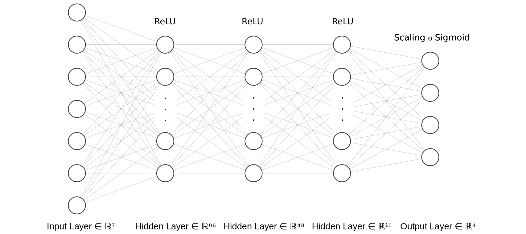
Figure 9: The architecture of the ANN consists of three hidden layers followed by the ReLU activation function and an output layer that uses the Sigmoid activation function in combination with a scaling function. In this particular case, we have $N_{D}=7$, $N_{L}=4$ and $N_{\theta}=4$. The calculation of the total number of trainable parameters for this architecture is detailed in Table 3.

Table 3: Number of parameters of the ANN where $N_{D}=7$, $N_{L}=4$ and $N_{\theta}=4$.

	Hidden layer 1	Hidden layer 2	Hidden layer 3	Output layer
Input shape	$(N_{D},\;)$	$(96,\;)$	$(48,\;)$	$(16,\;)$
Number of neurons	$96$	$48$	$16$	$N_{\theta}$
Number of parameters	$N_{D}.96+96=768$	$96.48+48=4656$	$48.16+16=784$	$16.N_{\theta}+N_{\theta}=68$
Total parameters: $6276$.

Let us consider an ensemble of layers where each layer is associated with its weight $\boldsymbol{W}_{j}$ and bias $\boldsymbol{b}_{j}$. Then, an input $I$ of each layer is mapped to the input of the next layer by a linear function $\phi_{j}(I)=\boldsymbol{W}_{j}I+\boldsymbol{b}_{j}$, and followed by the ReLU activation function denoted $\delta$, except for the last layer, which is followed by the Sigmoid activation function denoted $\sigma$, ensuring that its outputs are between 0 and 1. Now an output $\boldsymbol{O}_{x}=\sigma\circ\phi_{N_{L}}(.,x)\in[0,1]^{N_{\theta}}$ of the last layer is mapped to the range of the hydrological model parameters by a differentiable scaling function $s$:

$$\boldsymbol{\theta}(x)=s(\boldsymbol{O}_{x})=l+(u-l)\odot\boldsymbol{O}_{x}$$ (11)

where $l=\left(l_{1},...,l_{N_{\theta}}\right)$ and $u=\left(u_{1},...,u_{N_{\theta}}\right)$ with the lower and upper bounds $l_{k}\in\mathbb{R}$ and $u_{k}\in\mathbb{R}$, assumed spatially uniform, defining the bound constraints of $\theta_{k}(x),\forall(k,x)\in[1..N_{\theta}]\times\Omega$, in the direct hydrological model. The notation “$\odot$” denotes the Hadamard product.

Noting $\Psi_{j}\equiv\begin{cases}\delta\circ\phi_{j}\text{, }j=1..N_{L}-1\\ \sigma\circ\phi_{j}\text{, }j=N_{L}\end{cases}$, the forward propagation of the neural network $\mathcal{N}$ is defined as Equation 12.

$$\boldsymbol{\theta}(x)=\mathcal{N}(\boldsymbol{D}(x),.)=s\circ\Psi_{N_{L}}\circ\Psi_{N_{L}-1}\circ...\circ\Psi_{1}(\boldsymbol{D}(x)),\forall x\in\Omega.$$ (12)

Here, the notation “$\circ$” denotes the function composition operator.

Recall that our objective is the calibration problem of Equation 9 with respect to the regional control vector $\boldsymbol{\rho}\coloneqq\left[\boldsymbol{W},\boldsymbol{b}\right]$, using the cost function of Equation 10. In such manner, different variants of stochastic gradient descent algorithm are used and thus require the gradients of the cost function with respect to the weights and biases $\frac{\partial J}{\partial\boldsymbol{\rho}_{j}}$ for each layer, where $\boldsymbol{\rho}_{j}\coloneqq[\boldsymbol{W}_{j},\boldsymbol{b}_{j}]$. Since the forward model $\mathcal{M}\equiv\mathcal{M}_{rr}\left(.,\mathcal{N}\left(.\right)\right)$ with $\boldsymbol{\theta}$ being both the output of $\mathcal{N}$ and the input of $\mathcal{M}_{rr}$, we can write $\frac{\partial J}{\partial\boldsymbol{\rho}_{j}}=\frac{\partial J}{\partial\boldsymbol{\theta}}\frac{\partial\boldsymbol{\theta}}{\partial\boldsymbol{\rho}_{j}}$. Then these two gradients are obtained as follows:

• The gradients $\frac{\partial J}{\partial\boldsymbol{\theta}}$ of the cost function with respect to the hydrological model parameters, computed by solving the numerical adjoint model of $\mathcal{M}_{rr}$;

• The gradients $\frac{\partial\boldsymbol{\theta}}{\partial\boldsymbol{\rho}_{j}}$ of the network output with respect to the weight and bias, computed using the chain rule of composite functions of $\mathcal{N}$.

Eventually, the backward propagation for updating the weights and biases, using for instance Adam optimizer, is described in Algorithm 1.

Algorithm 1 Adapted back-propagation using Adam optimizer

$\vartriangleright$ Randomly initialized weights and biases $\boldsymbol{\rho}^{(0)}=\left(\boldsymbol{\rho}^{(0)}_{1},...,\boldsymbol{\rho}^{(0)}_{N_{L}}\right)$

$\vartriangleright$ Number of training iterations $N_{ite}$

  for $i=1..N_{ite}$ do

     $\vartriangleright$ Forward propagation over the spatial domain $\boldsymbol{\theta}\leftarrow\left[\left(\mathcal{N}\left(\boldsymbol{D}(x),\boldsymbol{\rho}^{(i-1)}\right)\right)_{x\in\Omega}\right]^{T}$

     $\vartriangleright$ Initial gradient accumulation $\nabla A\leftarrow\nabla_{\boldsymbol{\theta}}J=\left(\frac{\partial J}{\partial\theta_{1}},...,\frac{\partial J}{\partial\theta_{N_{\theta}}}\right)$

     for $j=N_{L}..1$ do

        $\vartriangleright$ Gradient computation $\frac{\partial J}{\partial\boldsymbol{\rho}_{j}}\leftarrow\left(\frac{\partial\boldsymbol{\theta}}{\partial\boldsymbol{\rho}_{j}}\right)^{T}\nabla A$

        $\vartriangleright$ Updated gradient accumulation $\nabla A\leftarrow\nabla A.\left[W_{j}^{(i-1)}\right]^{T}$

        $\vartriangleright$ Updated weights and biases $\boldsymbol{\rho}^{(i)}_{j}\leftarrow\boldsymbol{\rho}^{(i-1)}_{j}-\eta\frac{m^{(i)}}{(1-\beta_{1})\left(\sqrt{\frac{v^{(i)}}{1-\beta_{2}}}+\epsilon\right)}$ where:$m^{(i)}\leftarrow\beta_{1}m^{(i-1)}+(1-\beta_{1})\frac{\partial J}{\partial\boldsymbol{\rho}_{j}}\left(\boldsymbol{\rho}_{j}^{(i-1)}\right)$ $v^{(i)}\leftarrow\beta_{2}v^{(i-1)}+(1-\beta_{2})\left(\frac{\partial J}{\partial\boldsymbol{\rho}_{j}}\left(\boldsymbol{\rho}_{j}^{(i-1)}\right)\right)^{2}$ $\beta_{1}=0.9$ and $\beta_{2}=0.999$ are the decay rates for first and second moments of gradients $\epsilon=10^{-8}$ is a small scalar $\eta$ is the learning rate that is a tuning parameter determining the step size of the optimization problem

     end for

  end for

Appendix C Calibration results in case of Ardèche

This section provide several calibration/validation results obtained in the Ardèche area.

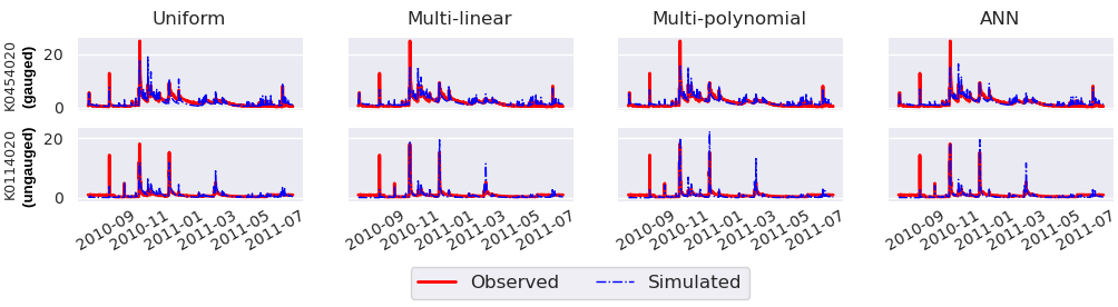
Figure 10: Study area: Ardèche. One year of observed and simulated discharges (in $m^{3}/s$) obtained with four multi-gauge regional calibration methods at one gauged (K0454020) and one pseudo-ungauged catchment (K0114020).

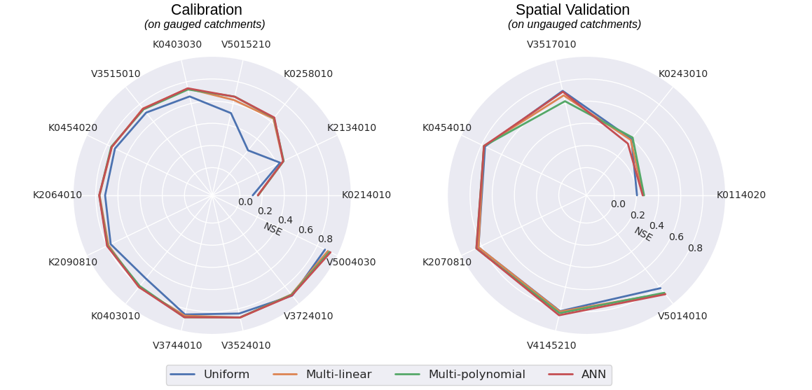
Figure 11: Study area: Ardèche. Radial plots of the NSE (optimal value = 1) in gauged catchments (left) and pseudo-ungauged catchments (right) during the calibration period for four multi-gauge regional calibration methods.

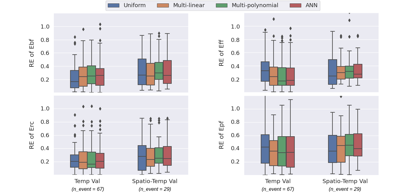
Figure 12: Study area: Ardèche. Relative error (RE, optimal value = 0) of 4 flood event signatures: base flow (Ebf), flood flow (Eff), runoff coefficient (Erc), peak flow (Epf), evaluated using $n\_event=67$ flood events at gauged catchments for temporal validation (Temp Val) and $n\_event=29$ flood events at pseudo-ungauged catchments for spatio-temporal validation (Spatio-Temp Val).

The proposed algorithms were implemented into the SMASH platform, which is interfaced in Python (Jay-Allemand et al., 2022a). The SMASH source code is licensed under GPL-3.0 and can be accessed at: https://github.com/DassHydro-dev/smash. Additionally, the code for conducting the numerical experiments and analysis in this study is licensed under MIT and provided at: https://github.com/nghi-truyen/Regionalization-Learning.