Are Easy Data Easy (for K-Means)

Abstract

This paper investigates the capability of correctly recovering well-separated clusters by various brands of the $k$-means algorithm. The concept of well-separatedness used here is derived directly from the common definition of clusters, which imposes an interplay between the requirements of within-cluster-homogenicity and between-clusters-diversity. Conditions are derived for a special case of well-separated clusters such that the global minimum of $k$-means cost function coincides with the well-separatedness. An experimental investigation is performed to find out whether or no various brands of $k$-means are actually capable of discovering well separated clusters. It turns out that they are not. A new algorithm is proposed that is a variation of $k$-means++ via repeated subsampling when choosing a seed. The new algorithm outperforms four other algorithms from $k$-means family on the task.

I Introduction

As visible from majority of papers (see e.g. [23], [8]), clustering is most frequently understood as splitting data into several subsets such that each of these clusters consists of data objects with high intra-cluster-similarity and low inter-cluster-similarity. We investigate in this paper the behaviour of algorithms from the $k$-means family under this favourable assumption. $k$-means is one of the most famous clustering algorithms invented more than half a century. Thanks to a multitude optimization and enhancement works, $k$-means is also the most popular clustering algorithm in use in various domains. For recent overviews of various brands of this algorithm see e.g. [4] or [27].

If we take seriously the assumption of high intra-cluster-similarity and low inter-cluster-similarity, then the distance of a datapoint to other datapoints of the same cluster should be lower than the distance of the same datapoint to datapoints of other clusters. This assumption fits the definition of so-called nice clustering [1]. If we push further and require that the minimum separation between clusters be larger than the maximum cluster diameter, then we speak about perfect clustering [1]. If we extend this requirement not only to datapoints but to the entire hyperballs centered at cluster gravity center and encompassing all cluster datapoints, then we speak about perfect-ball-clustering [18]. Provably, incremental $k$-means algorithm introduced in [1], can discover the perfect ball clustering if it exists [18] and if we know the correct number of clusters in advance. It shall be stressed, however, that incremental $k$-means does not seek to optimize the traditional $k$-means cluster quality function.

This paper presents a study of $k$-means properties when dealing with this most simplistic case of clusters. The merit of studying such a trivial case of clustering is two-fold. First, the concept of a cluster is not so clear in general, as one may expect. So the study of clustering should start with conceptual investigation of the case when the concept seems to be clear-cut. Second, it turns out that the well-studied and widely applied $k$-means algorithm may fail under these ideal circumstances. We point at an algorithm based on $k$-means that is well suited under such circumstances. We hope that it may constitute a hint for elaboration of some in-between versions for leaning $k$-means towards human cluster expectations.

As the $k$-means family of clustering algorithms is astoundingly large, [4], [27], we have selected only a few representatives for this study: the traditional $k$-means [21], $k$-means++ [3] [25], ”most distant initialization” algorithm [19], global $k$ means (GKM) [20] and our own variation. These algorithms seem to be representative for diverse ideas on algorithm initialization which is essential for well-separated data (as this study confirms).

II Previous work

The widely used $k$-means clustering algorithm ([21], for various versions see e.g. [27]) seeks, for a dataset $\mathbf{X}$, to minimize the function

$$Q(\Gamma)=\sum_{i=1}^{m}\sum_{j=1}^{k}u_{ij}\|\textbf{x}_{i}-\boldsymbol{\mu}_{j}\|^{2}=\frac{1}{2}\sum_{j=1}^{k}\frac{1}{n_{j}}\sum_{\mathbf{x}_{i}\in C_{j}}\sum_{\mathbf{x}_{l}\in C_{j}}\|\mathbf{x}_{i}-\mathbf{x}_{l}\|^{2}$$ (1)

under some partition $\Gamma$ into $k$ clusters, where $u_{ij}$ is an indicator ($u_{ij}\in\{0,1\}$) of the membership of data point $\textbf{x}_{i}$ in the cluster $C_{j}$ having the center at $\boldsymbol{\mu}_{j}$.

We will call $k$-means-ideal such an algorithm that finds a $\Gamma_{opt}$ that attains the minimum of function $Q(\Gamma)$. It is known that it is a hard task.

Many researchers try to approximate $k$-means-ideal within a reasonable error bound (e.g. $9+\epsilon$ by [9]), via cleverly initiated $k$-means type algorithms, (e.g. $k$-means++ [3] [25], or ”most distant initialization” algorithm which is claimed to be nearly as effective as $k$-means++ [19]), or other algorithms, like (robust) single link, or approximating the quality function value by using a higher $k^{\prime}$ when clustering. Recently, attention of the researchers was attracted by the so-called global $k$ means (GKM) [20] due to its successes in finding quite well initial seeds for $k$-means in a more deterministic way than in the other algorithms, which has a number of follow-ups aiming at improving its efficiency (see e.g. [7], [5] , [2] and many other).

The $k$-means like algorithms are of interest not only because their efficiency, but also due to interesting theoretical property like consistency in the limit for growing sample sizes [12], applicability of kernel-trick for Euclidean [11] and non-Euclidean space [16], existence of cluster-preserving transformations [13], possibility to check clusterability [14], applicability in label-free test set evaluations [22], privacy preserving [26] and many other [10], [17], [15]. Therefore, intense studies of $k$-means family are vital.

The $k$-means clustering of well-separated data is a topic studied in the context of diverse applications [6], [24]. In various publications (including [24]), assumptions are possibly made about the structure of the data, e.g. about sufficiently large gaps between the clusters, or low variance compared to cluster center distances etc. We will pursue here this line of research by investigating the capability of $k$-means like algorithm to discover well separated clusters.

In this paper, we will use $k$-means implementation in $R$, which allows to investigate several brands of algorithms from this family differing on the way it is initialized.

III The Easy Case for $k$-Means

Recall that $k$-means is intended to cluster a dataset $D$ into the set $\Gamma$ of $k$ non-empty non-intersecting groups, called clusters such that they should reach the minimum of the $k$-means cost function, Eq. (1), that may be reformulated as:

$$Q(\Gamma,d)=\sum_{C\in\Gamma}\sum_{i\in C}\sum_{j\in C}d^{2}(i,\boldsymbol{\mu}(C))$$

where $\boldsymbol{\mu}(C)$ is the position of the center of gravity of cluster C, and $d$ is the (Euclidean) distance induced by the embedding of $D$ in some $\mathbb{R}^{m}$. The ideal-$k$-means is one that reaches this minimum, by discovering $\Gamma_{true}$ (but with prohibitive execution time), while there exist multiple implementations, real-$k$-means algorithms that find some $\Gamma$ approximating this goal only (sticking in some local minimum of $Q(\Gamma$)

Consider a dataset $D$, and its intended clustering $\Gamma_{I}$ into $k$ clusters such that each $C\in\Gamma$ has the same cardinality ($|C|=n$). We seek for conditions under which $\Gamma_{I}=\Gamma_{true}$. To this end, we assume that each cluster $C\in\Gamma_{I}$ can be enclosed into a (hyper)ball of radius $R$ with center at $\boldsymbol{\mu}(C)$, for some fixed $R$. Furthermore there exist a $g$ such that distances between various mentioned ball surfaces amount to at least $g$. We will impose restrictions on $g$.

Under these circumstances consider a clustering $\Gamma$ of $D$, obtained by some real $k$-means. The first possibility is that each $\boldsymbol{\mu}(C)$ for each $C$ in $\Gamma$ lies outside of each $C_{I}\in\Gamma_{I}$ at a distance over $R$ from the surface. In this case $Q(\Gamma_{I},d)<Q(\Gamma,d)$, hence $\Gamma$ is not optimal.

Let us discuss other case that is there exists at least one cluster $C_{N}\in\Gamma_{I}$ such that some $\boldsymbol{\mu}(C_{1})$, $C_{1}\in\Gamma$ is at the distance at most $R$ from the ball of $C_{N}$. This means that for each $e\in C_{N}$: $d(e,\boldsymbol{\mu}(C_{1}))\leq 3R$. Let $z\in C_{2}\cap C_{N}$ where $C_{T}\in\Gamma_{I},C_{T}\neq C_{N}$ and there exists a $C_{2}\in\Gamma$ such that $\boldsymbol{\mu}(C_{2})$ is at most $R$ away from $C_{T}$ ball. Then $d(z,\boldsymbol{\mu}(C_{1}))>g-R$. If $g>4R$, then $d(z,\boldsymbol{\mu}(C_{1}))>3R\geq d(z,\boldsymbol{\mu}(C_{2}))$ and therefore for $\Gamma^{\prime}$ such that $\Gamma^{\prime}=(\Gamma/\{C_{1},C_{2}\})\cup\{C_{1}/\{z\},C_{2}\cup\{z\}\}$ we have $Q(\Gamma^{\prime},d)<Q(\Gamma,d)$, hence $\Gamma$ is not optimal.

So let us discuss the case excluding the above that implies the situation where for each $C\in\Gamma$ such that if $\boldsymbol{\mu}(C)$ is at most $R$ away from some ball of $C_{N}\in\Gamma_{I}$, then each element $e$ of $C_{N}$ for each $C_{2}\in\Gamma$: $d(e,\boldsymbol{\mu}(C_{2}))>3R$.

We can have two cases: either each $C_{N}\in\Gamma_{I}$ has exactly one $C\in\Gamma$ such that $\boldsymbol{\mu}(C)$ is at most $R$ away from $C_{N}$ ball or some $C_{N}\in\Gamma_{I}$ have at least one $C\in\Gamma$ such that $\boldsymbol{\mu}(C)$ is at most $R$ away from $C_{N}$ ball and other do not.

In the first case obviously $Q(\Gamma_{I},d)\leq Q(\Gamma,d)$ because each element of a close cluster that is not in the intended cluster to which it is close, is further away from the cluster center than if it would be if moved to the close cluster to its intended cluster.

In the second let us distinguish close $\boldsymbol{\mu}(C)$’s as such that are at most $R$ away from some intended cluster ball (and the respective $C$s will be called close clusters) and the other $\boldsymbol{\mu}(C)$’s that shall be called ”remote” (and the respective $C$s will be called remote clusters). An intended cluster ball with a $\boldsymbol{\mu}(C)$ not further than $R$ away from it will be called ”with satellite”, while the other ”without satellite”.

Let us denote the set of all elements that belong to a close cluster but do not belong to the respective intended cluster with satellite with $A_{c}$. For each element $e$ of $A_{c}$, belonging to some $C_{T}\in\Gamma_{I}$ and some $C\in\Gamma$ its distance to $\boldsymbol{\mu}(C)$ is at least $g-R$, and its distances to all the other cluster centers of $\Gamma$ amount to at least to $g-3R$. All other elements of $C_{T}$ have distances to cluster centers of $\Gamma$ not smaller than $g-3R$. There exists at least one such cluster $C_{T}$. There exist clearly at most $k-1$ close clusters. If we switch to $\Gamma_{I}$ from $\Gamma$, then in these clusters the overall contribution to $Q$ may increase at most by $R^{2}(k-1)n$. The contribution of the mentioned remote cluster $C_{T}$ (there exists at least one such cluster) will decrease at least by $(g-3R)^{2}n$. For all the other remote clusters the contribution will for sure not increase. Therefore, if we are interested in having $Q(\Gamma_{I},d)<Q(\Gamma,d)$, it will be sufficient to have: $R^{2}(k-1)n<(g-3R)^{2}n$. Hence $R^{2}(k-1)<(g-3R)^{2}$. $R\sqrt{k-1}<g-3R$ $R(\sqrt{k-1}+3)<g$. So two conditions have to hold: $g>4R$ and $g>R(\sqrt{k-1}+3)$. The first is superfluous as usually we have at least two clusters to consider.

In 2D on the grid, there are not $k-1$ but rather only at most 8 neighbours of $C_{T}$ to consider. So we will be working with $g>R(\sqrt{8}+3).$

Out of these considerations, we can formulate theorems:

Theorem 1

For a clustering $\Gamma$ (embedded in Euclidean space) such that each cluster can be enclosed in a ball with radius $R$ centered at its gravity center and the distances between the enclosing balls are at least $R(\sqrt{k-1}+3)$, where $k=|\Gamma|$m, then $\Gamma$ minimizes the cost function (1).

Theorem 2

If the clustering from the previous theorem is embedding in two-dimensional space, then it is sufficient that the distances between enclosing balls are not smaller than $R(\sqrt{8}+3)$

IV Experiments

The goal of our experiments is to see whether or not various brands of $k$-means can discover the optimal clustering for well separated data (easy conditions). We investigate clusters lying on a regular grid, clusters slightly dislocated from regular grid, data without noise and data with noise. Various sizes of clusters will be investigated.

IV-A Data

Two-dimensional synthetic data will be used. The minimum distance between clusters is taken from Theorem 2. All clusters will be of the same size. In various experiments this size will vary from 12 to 06. The number of clusters vary from 25 to 100.

Each element of a cluster is generated as follows: From the intended cluster center take a random direction (uniform sampling) and then sample uniformly the distance from intended cluster center (from zero to cluster radius). The noise is generated in the same way, with the exception that the distance from the intended cluster center is radius plus sample from Gaussian distribution (with standard deviation equal cluster radius).

All cluster radii are identical. Clusters are placed on regular grids. Distortion of cluster center position is taken uniformly from, the assumed range.

Synthetic data is used because to the best of our knowledge no real data sets with guaranteed global minimum of $k$-means cost function exist (only datasets are known for which no better solution was found in spite of computational effort).

IV-B Methods

Data: $D$ - a set of objects embedded in Euclidean space (that is for each $i\in D$ there exists its representation $\mathbf{x_{i}}$ in Euclidean space), to be clustered

$k$ - the number of clusters to be returned

Result: $\Gamma$ - the clustering of $D$ into $k$ clusters

Initialize the set $M$ of $k$ cluster centers - step depends of the concrete algorithm;

while termination not reached do

       Create a clustering $\Gamma$ assigning to each $\boldsymbol{\mu}\in M$ the subset of $D$ of elements closest to $\boldsymbol{\mu}$ ; Drop $M$ and create a new one such that for each cluster $C\in\Gamma$ compute $\boldsymbol{\mu}(C)=\frac{1}{|C|}\sum_{i\in C}\mathbf{x_{i}}$;

      

end while

return $\Gamma$;

Algorithm 1 The framework of the various brands of $k$-means algorithms; termination condition may be a fixed number of loop runs or no change of clustering within a loop run.

Data: $D$ - a set of objects embedded in Euclidean space, to be clustered

$k$ - the number of clusters to be created

Result: $M$ - the set of initial centroids to be used in the k$-means$

Pick $M$ as a random sample of $k$ elements from $D$ without repetition;

return $M$;

Algorithm 2 The initialization for the $k$-means algorithm, used in conjunction with Algorithm 1.

Data: $\Gamma$ - the intended clustering

$k$ - the number of clusters to be created ($|\Gamma|=k$ required

Result: $M$ - the set of initial centroids to be used in the $tc-$k$-means$

Create $M$ such that for each cluster $C\in\Gamma$ compute $\boldsymbol{\mu}(C)=\frac{1}{|C|}\sum_{i\in C}\mathbf{x_{i}}$;

return $M$;

Algorithm 3 The initialization for the tc-$k$-means algorithm, used in conjunction with Algorithm 1.

Data: $D$ - a set of objects embedded in Euclidean space, to be clustered

$k$ - the number of clusters to be created

Result: $M$ - the set of initial centroids to be used in the k$-means$

Pick one element of $D$ at random and initialize $M$ with it. ;

for $j\leftarrow 2$ to $k$ by $1$ do

       Assign to each element of $e\in D$ a probability $p_{e}$, proportional to the squared distance of $e$ to the closest element of $M$;

       Sample one element $c\in D$ according to the above-mentioned probability; $M\leftarrow=M\cup\{c\}$

end for

return $M$;

Algorithm 4 The initialization for the $k$-means++ algorithm, used in conjunction with Algorithm 1.

Data: $D$ - a set of objects embedded in Euclidean space, to be clustered

$k$ - the number of clusters to be created

Result: $M$ - the set of initial centroids to be used in the k$-means$

Pick one element of $D$ at random and initialize $M$ with it. ;

for $j\leftarrow 2$ to $k$ by $1$ do

       Find the element $c\in D$ with the highest distance to the closest element of $M$. ;

       $M\leftarrow=M\cup\{c\}$

end for

return $M$;

Algorithm 5 The initialization for the md-$k$-means algorithm, used in conjunction with Algorithm 1.

Data: $D$ - a set of objects embedded in Euclidean space, to be clustered

$k$ - the number of clusters to be created

$b$ - boosting parameter

Result: $M$ - the set of initial centroids to be used in the k$-means$

Pick one element of $D$ at random and initialize $M$ with it. for $j\leftarrow 2$ to $k$ by $1$ do

       Assign to each element of $e\in D$ a probability $p_{e}$, proportional to the squared distance of $e$ to the closest element of $M$;

       Sample $b$ elements $B\subset D$ according to the above-mentioned probability; Select the element $c\in B$ for which the sum of distances of all elements of $D$ to the closest element from the set $M\cup\{c\}$ is the lowest;

       $M\leftarrow=M\cup\{c\}$;

      

end for

return $M$;

Algorithm 6 The initialization for the $k$-means++B algorithm, used in conjunction with Algorithm 1.

Data: $D$ - a set of objects embedded in Euclidean space, to be clustered

$k$ - the number of clusters to be created

Result: $M$ - the set of initial centroids to be used in the k$-means$

Initialize $M$ with the centroid of $D$;

for $j\leftarrow 2$ to $k$ by $1$ do

       For each $e\in D$ compute the statistics $v_{e}=\sum_{f\in D}\max\left(0,d^{2}(f,M)-d^{2}(f,e)\right)$$; Select the element $c\in D$ such that $v_{c}$ takes on the maximum value (maximum reduction of errors);

       $M\leftarrow M\cup\{c\}$;

      

end for

return $M$;

Algorithm 7 The initialization for the glob-$k$-means algorithm, used in conjunction with Algorithm 1.

We will subsequently investigate the following versions of $k$-means:

• the original $k$-means with random initialization ($k$-means),[21], see Algorithm 2.

• the $k$-means++ with probabilistic seeding with probabilities proportional to squared distances to already selected seeds ($k$-means++), ([3]), see Algorithm 4.

• a boosted version of the $k$-means++, proposed in this paper ($k$-means++B), see Algorithm 6; the parameter $b$ is set to 15 through all experiments.

• global $k$-means (glob-$k$-means, [7], [5], [2]), see Algorithm 7.

• most distant seed $k$-means (md-$k$-means), initialized by choosing the seed most distant to existing seeds, [19], see Algorithm 5

• unrealistic ”true center” $k$-means, seeded with true cluster centers (tc-$k$-means), see Algorithm 3.

TABLE I: Misclustering errors for the number of clusters $k$= 5 x 5 = 25 noise level= 0 %, cluster radius= 10 , cluster size= 40 , motion freedom of clusters= 0 , minimal distance between clusters: 5.83 *R

	SS	sd	BC%	sd	relSS	sd
$k$-means	245190.2	73349.84	21.07	7.37	7.57	2.3
tc-$k$-means	32429.34	899.34	0	0	1	0
md-$k$-means	32429.34	899.34	0	0	1	0
glob-$k$-means	32429.34	899.34	0	0	1	0
$k$-means++	93007.96	74481.14	6	7.43	2.87	2.31
$k$-means++B	32429.34	899.34	0	0	1	0

TABLE II: Misclustering errors for the number of clusters $k$= 6 x 6 = 36 noise level= 0 %, cluster radius= 10 , cluster size= 40 , motion freedom of clusters= 0 , minimal distance between clusters: 5.83 *R

	SS	sd	BC%	sd	relSS	sd
$k$-means	418367.7	67462.19	24.35	4.46	8.93	1.48
tc-$k$-means	46884.35	1036.28	0	0	1	0
md-$k$-means	46884.35	1036.28	0	0	1	0
glob-$k$-means	46884.35	1036.28	0	0	1	0
$k$-means++	140119.3	101557.5	6.39	7.03	3	2.18
$k$-means++B	46884.35	1036.28	0	0	1	0

TABLE III: Misclustering errors for the number of clusters $k$= 7 x 7 = 49 noise level= 0 %, cluster radius= 10 , cluster size= 40 , motion freedom of clusters= 0 , minimal distance between clusters: 5.83 *R

	SS	sd	BC%	sd	relSS	sd
$k$-means	608395.6	84216.04	26.33	3.74	9.51	1.38
tc-$k$-means	64029.5	1054.86	0	0	1	0
md-$k$-means	64029.5	1054.86	0	0	1	0
glob-$k$-means	64029.5	1054.86	0	0	1	0
$k$-means++	209584.8	96739.58	7.34	4.85	3.27	1.5
$k$-means++B	64029.5	1054.86	0	0	1	0

TABLE IV: Misclustering errors for the number of clusters $k$= 8 x 8 = 64 noise level= 0 %, cluster radius= 10 , cluster size= 40 , motion freedom of clusters= 0 , minimal distance between clusters: 5.83 *R

	SS	sd	BC%	sd	relSS	sd
$k$-means	839627.6	113618.2	28.23	4.11	10.12	1.41
tc-$k$-means	83059.99	1565.39	0	0	1	0
md-$k$-means	83059.99	1565.39	0	0	1	0
glob-$k$-means	83059.99	1565.39	0	0	1	0
$k$-means++	269336.8	139768.3	7.19	5.38	3.24	1.67
$k$-means++B	83059.99	1565.39	0	0	1	0

TABLE V: Misclustering errors for the number of clusters $k$= 9 x 9 = 81 noise level= 0 %, cluster radius= 10 , cluster size= 40 , motion freedom of clusters= 0 , minimal distance between clusters: 5.83 *R

	SS	sd	BC%	sd	relSS	sd
$k$-means	1121321	115220.7	29.55	2.97	10.67	1.1
tc-$k$-means	105069.2	1628.07	0	0	1	0
md-$k$-means	105069.2	1628.07	0	0	1	0
glob-$k$-means	105069.2	1628.07	0	0	1	0
$k$-means++	334273.7	110026.9	7.04	3.36	3.18	1.04
$k$-means++B	105069.2	1628.07	0	0	1	0

TABLE VI: Misclustering errors for the number of clusters $k$= 10 x 10 = 100 noise level= 0 %, cluster radius= 10 , cluster size= 40 , motion freedom of clusters= 0 , minimal distance between clusters: 5.83 *R

	SS	sd	BC%	sd	relSS	sd
$k$-means	1452519	133942.8	30.93	3.26	11.2	0.94
tc-$k$-means	129623.5	2345.05	0	0	1	0
md-$k$-means	129623.5	2345.05	0	0	1	0
glob-$k$-means	129623.5	2345.05	0	0	1	0
$k$-means++	449299.6	148633.3	7.9	3.67	3.47	1.15
$k$-means++B	129623.5	2345.05	0	0	1	0

IV-C Evaluation

The quality of the algorithms is evaluated as follows. Thirty times a data sample is generated, eventually with addition of noise. Then each algorithm is run of the same data sample. The following quantities are computed: SS - total sum of squared distances between elements and the discovered cluster centers, BC% - the percentage of intended clusters, that were not discovered by the algorithm (only regular data points are considered, noise is neglected), relSS - the relative SS, that is SS of a given algorithm divided by the lowest SS among algorithms for a given dataset.

The presented tables contain + for each of the above three criteria + the average over 30 datasets (30 runs) and the standard deviation (column denoted as SD). Additionally, the worst cases (with the highest BC%) are stored. Selected worst cases are presented in the accompanying figures. The discovered clusters differ in color and mark shapes. The erroneous discovered clusters are mark with big black circle.

IV-D Clusters on regular grid without noise

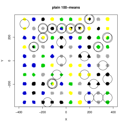
Figure 1: Worst misclustering errors $k$-means for the number of clusters $k$= 10 x 10 = 100 noise level= 0 %, cluster radius= 10 , cluster size= 40 , motion freedom of clusters= 0 , minimal distance between clusters: 5.83 *R

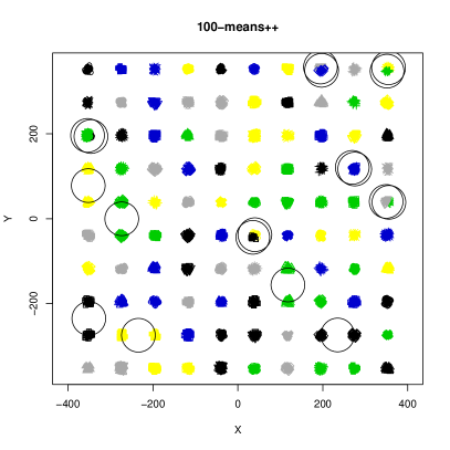
Figure 2: Worst misclustering errors $k$-means++ for the number of clusters $k$= 10 x 10 = 100 noise level= 0 %, cluster radius= 10 , cluster size= 40 , motion freedom of clusters= 0 , minimal distance between clusters: 5.83 *R

The results of the experiment in discovering correctly clusters lying on a regular grid without noise are presented in tables I, II, III, IV, V and VI for $k=25,36,49,64,81,100$ resp. As visible, all the algorithms detect the true clustering except for $k$-means and $k$-means++. The $k$-means++ performs significantly better than the baseline $k$-means, and the percentage of errors of $k$-means++ increases insignificantly when increasing the number of clusters by the factor of four, while $k$-means increases the error rate by 50%. Sample worst cases for the algorithms can be seen in figures 1 and 2. The circles indicate the erroneous clusters. Each circle is centered at the gravity center of the detected cluster. So if two circles overlap, then it means that a true cluster was split into two (or more) clusters (there are six such cases in figures 1).. If a circle touches two true clusters then it means that the algorithm failed to recognize that there are two clusters (six such cases in figures 1).

.

IV-E Clusters on regular grid with noise

TABLE VII: Misclustering errors for the number of clusters $k$= 8 x 8 = 64 noise level= 10 %, cluster radius= 10 , cluster size= 40 , motion freedom of clusters= 0 , minimal distance between clusters: 5.83 *R

	SS	sd	BC%	sd	relSS	sd
$k$-means	898477.4	107564.2	24.93	3.84	10.59	1.29
tc-$k$-means	84862.53	1680.56	0	0	1	0
md-$k$-means	92855.78	29994.68	0.26	1	1.09	0.35
glob-$k$-means	206743.7	3301.28	3.17	NaN	2.44	0.04
$k$-means++	352599	141800	9.98	5.45	4.16	1.7
$k$-means++B	84863.96	1681.49	0	0	1	0

TABLE VIII: Misclustering errors for the number of clusters $k$= 8 x 8 = 64 noise level= 20 %, cluster radius= 10 , cluster size= 40 , motion freedom of clusters= 0 , minimal distance between clusters: 5.83 *R

	SS	sd	BC%	sd	relSS	sd
$k$-means	978119.1	132268.8	23.56	3.56	11.48	1.54
tc-$k$-means	85174.19	1377.86	0	0	1	0
md-$k$-means	93401.87	30463.09	0.31	1.17	1.1	0.37
glob-$k$-means	204133.2	22354.87	3.06	0.57	2.4	0.26
$k$-means++	348469.3	112942.2	9.64	4.26	4.1	1.34
$k$-means++B	85175.5	1376.77	0	0	1	0

TABLE IX: Misclustering errors for the number of clusters $k$= 8 x 8 = 64 noise level= 30 %, cluster radius= 10 , cluster size= 40 , motion freedom of clusters= 0 , minimal distance between clusters: 5.83 *R

	SS	sd	BC%	sd	relSS	sd
$k$-means	1080724	99859.57	23.15	2.66	12.69	1.27
tc-$k$-means	85278.66	1548.65	0	0	1	0
md-$k$-means	134501	75551.75	1.58	2.47	1.57	0.88
glob-$k$-means	207550.5	3081.93	3.17	NaN	2.43	0.04
$k$-means++	416564.9	128271.7	11.68	4.62	4.89	1.5
$k$-means++B	85275.53	1542.16	0	0	1	0

TABLE X: Misclustering errors for the number of clusters $k$= 8 x 8 = 64 noise level= 40 %, cluster radius= 10 , cluster size= 40 , motion freedom of clusters= 0 , minimal distance between clusters: 5.83 *R

	SS	sd	BC%	sd	relSS	sd
$k$-means	1162857	118303.5	22.2	3.35	13.55	1.37
tc-$k$-means	85807.74	1429.99	0	0	1	0
md-$k$-means	135133.9	74748.25	1.68	2.63	1.58	0.87
glob-$k$-means	208272.4	3781.91	3.17	NaN	2.43	0.04
$k$-means++	437003.7	126730	12.39	4.48	5.09	1.46
$k$-means++B	85809.42	1430.65	0	0	1	0

TABLE XI: Misclustering errors for the number of clusters $k$= 8 x 8 = 64 noise level= 50 %, cluster radius= 10 , cluster size= 40 , motion freedom of clusters= 0 , minimal distance between clusters: 5.83 *R

	SS	sd	BC%	sd	relSS	sd
$k$-means	1304727	119562.3	23.05	3.07	15.06	1.32
tc-$k$-means	86632.72	1362.46	0	0	1	0
md-$k$-means	147695	68845.15	2.04	2.43	1.7	0.79
glob-$k$-means	205161.5	22190.22	3.12	0.64	2.37	0.26
$k$-means++	424568.7	123582.4	12.11	4.74	4.91	1.45
$k$-means++B	94858.91	30873.22	0.26	1	1.09	0.35

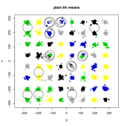
Figure 3: Worst misclustering errors $k$-means for the number of clusters $k$= 8 x 8 = 64 noise level= 30 %, cluster radius= 10 , cluster size= 40 , motion freedom of clusters= 0 , minimal distance between clusters: 5.83 *R

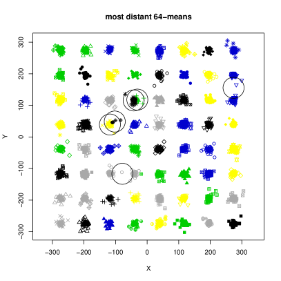
Figure 4: Worst misclustering errors md-$k$-means for the number of clusters $k$= 8 x 8 = 64 noise level= 30 %, cluster radius= 10 , cluster size= 40 , motion freedom of clusters= 0 , minimal distance between clusters: 5.83 *R

Figure 5: Worst misclustering errors $k$-means++ for the number of clusters $k$= 8 x 8 = 64 noise level= 30 %, cluster radius= 10 , cluster size= 40 , motion freedom of clusters= 0 , minimal distance between clusters: 5.83 *R

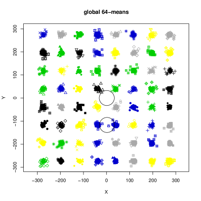
Figure 6: Worst misclustering errors glob-$k$-means for the number of clusters $k$= 8 x 8 = 64 noise level= 30 %, cluster radius= 10 , cluster size= 40 , motion freedom of clusters= 0 , minimal distance between clusters: 5.83 *R

The results of clustering on regular grid with noise ranging from 10 to 50% can be seen in tables VII - XI. All algorithms commit errors except for tc-$k$-means and $k$-means++B. Worst cases are presented in figures 3 - 6. The algorithms seem not to be much sensitive to noise (that is their error rate does not increase with noise much), in particular the $k$-means and $k$-means++. glob-$k$-means, which appears to perform worse than md-$k$-means in the experiments, nevertheless exhibits error stability, while md-$k$-means error increases systematically.

IV-F Clusters with positions disturbed with respect to a regular grid

The results of clustering on regular grid with noise and with dislocating clusters from grid points by 0.5 to 4 cluster radii can be seen in tables XII - XV. Algorithms $k$-means, $k$-means++ and glob-$k$-means commit errors. Worst cases are presented in figures 7 - 9.

TABLE XII: Misclustering errors for the number of clusters $k$= 8 x 8 = 64 noise level= 30 %, cluster radius= 10 , cluster size= 40 , motion freedom of clusters= 5 , minimal distance between clusters: 5.83 *R

	SS	sd	BC%	sd	relSS	sd
$k$-means	1324228	164858.9	24.78	3.98	15.39	1.93
tc-$k$-means	86053.02	1553.69	0	0	1	0
md-$k$-means	95193.42	33978.65	0.31	1.17	1.11	0.4
glob-$k$-means	207401.8	48454.39	2.75	1.08	2.41	0.56
$k$-means++	494330.4	151398.7	12.58	4.8	5.75	1.78
$k$-means++B	86053.02	1553.69	0	0	1	0

TABLE XIII: Misclustering errors for the number of clusters $k$= 8 x 8 = 64 noise level= 30 %, cluster radius= 10 , cluster size= 40 , motion freedom of clusters= 10 , minimal distance between clusters: 5.83 *R

	SS	sd	BC%	sd	relSS	sd
$k$-means	1695803	225108.9	28.52	4.04	19.71	2.55
tc-$k$-means	86016.3	1185.21	0	0	1	0
md-$k$-means	86016.3	1185.21	0	0	1	0
glob-$k$-means	218801.5	55080.32	2.75	1.08	2.54	0.64
$k$-means++	451174.5	218741.7	9.6	5.47	5.25	2.56
$k$-means++B	86016.3	1185.21	0	0	1	0

TABLE XIV: Misclustering errors for the number of clusters $k$= 8 x 8 = 64 noise level= 30 %, cluster radius= 10 , cluster size= 40 , motion freedom of clusters= 20 , minimal distance between clusters: 5.83 *R

	SS	sd	BC%	sd	relSS	sd
$k$-means	2510247	271035	35.27	3.71	29.36	3.18
tc-$k$-means	85506.64	1525.18	0	0	1	0
md-$k$-means	85506.64	1525.18	0	0	1	0
glob-$k$-means	197579.5	75928.16	2.22	1.45	2.31	0.89
$k$-means++	491747	241062.7	9.14	5.64	5.75	2.8
$k$-means++B	85506.64	1525.18	0	0	1	0

TABLE XV: Misclustering errors for the number of clusters $k$= 8 x 8 = 64 noise level= 30 %, cluster radius= 10 , cluster size= 40 , motion freedom of clusters= 40 , minimal distance between clusters: 5.83 *R

	SS	sd	BC%	sd	relSS	sd
$k$-means	4116153	479531.9	38.98	5.19	48.05	5.75
tc-$k$-means	85707.34	1508.97	0	0	1	0
md-$k$-means	85707.34	1508.97	0	0	1	0
glob-$k$-means	230218.6	85552.31	2.43	1.34	2.68	0.99
$k$-means++	470169.7	239104.3	6.89	3.79	5.48	2.75
$k$-means++B	85707.34	1508.97	0	0	1	0

One gets the impression that dislocation of clusters from grid positions improves the performance of all algorithms except for $k$-means. This improvement stems from the fact that allowing for dislocation enforces larger gaps between clusters so that the minimum gap from Theorem 2 is kept. This distance increase has however bad effects on $k$-means because it reduces its capability of recovery after a faulty seed initialization which is always the poorest among the algorithms.

Figure 7: Worst misclustering errors $k$-means for the number of clusters $k$= 8 x 8 = 64 noise level= 30 %, cluster radius= 10 , cluster size= 40 , motion freedom of clusters= 40 , minimal distance between clusters: 5.83 *R

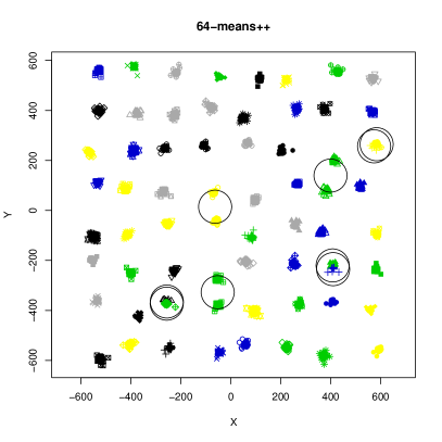
Figure 8: Worst misclustering errors $k$-means++ for the number of clusters $k$= 8 x 8 = 64 noise level= 30 %, cluster radius= 10 , cluster size= 40 , motion freedom of clusters= 40 , minimal distance between clusters: 5.83 *R

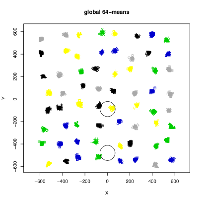
Figure 9: Worst misclustering errors glob-$k$-means for the number of clusters $k$= 8 x 8 = 64 noise level= 30 %, cluster radius= 10 , cluster size= 40 , motion freedom of clusters= 40 , minimal distance between clusters: 5.83 *R

IV-G Impact of cluster size on clustering

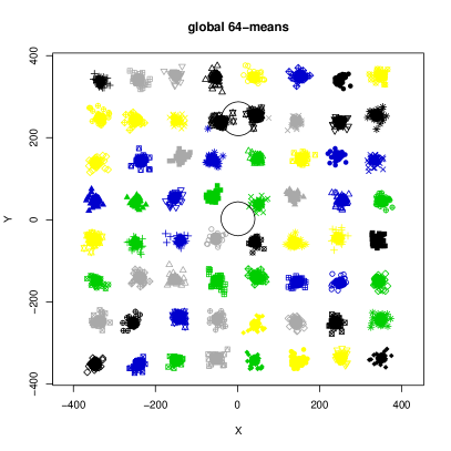
Figure 12: Worst misclustering errors glob-$k$-means for the number of clusters $k$= 8 x 8 = 64 noise level= 30 %, cluster radius= 10 , cluster size= 96 , motion freedom of clusters= 10 , minimal distance between clusters: 5.83 *R

The impact of cluster size on clustering can be seen in tables XVI - XIX. Here, the cluster sizes range from 12 to 96. All algorithms commit errors except for tc-$k$-means and $k$-means++B. Worst cases are presented in figures 10 - 12. No obvious pattern can be seen for error dependence on cluster size. Well-separatedness plays a dominant role.

TABLE XVI: Misclustering errors for the number of clusters $k$= 8 x 8 = 64 noise level= 30 %, cluster radius= 10 , cluster size= 12 , motion freedom of clusters= 10 , minimal distance between clusters: 5.83 *R

	SS	sd	BC%	sd	relSS	sd
$k$-means	532774.8	59062.4	26.9	4.59	20.21	2.32
tc-$k$-means	26384.5	888.86	0	0	1	0
md-$k$-means	26384.5	888.86	0	0	1	0
glob-$k$-means	56905.01	20166.2	2.22	1.45	2.17	0.78
$k$-means++	152971.8	48444.23	10.39	4.27	5.8	1.83
$k$-means++B	26384.5	888.86	0	0	1	0

TABLE XVII: Misclustering errors for the number of clusters $k$= 8 x 8 = 64 noise level= 30 %, cluster radius= 10 , cluster size= 24 , motion freedom of clusters= 10 , minimal distance between clusters: 5.83 *R

	SS	sd	BC%	sd	relSS	sd
$k$-means	1036702	92429.47	29.33	3.53	20.1	1.78
tc-$k$-means	51597.87	965.31	0	0	1	0
md-$k$-means	51596.23	961.13	0	0	1	0
glob-$k$-means	117913.5	40946.04	2.32	1.4	2.28	0.79
$k$-means++	255396.2	101449.6	8.32	4.28	4.95	1.95
$k$-means++B	51596.23	961.13	0	0	1	0

TABLE XVIII: Misclustering errors for the number of clusters $k$= 8 x 8 = 64 noise level= 30 %, cluster radius= 10 , cluster size= 48 , motion freedom of clusters= 10 , minimal distance between clusters: 5.83 *R

	SS	sd	BC%	sd	relSS	sd
$k$-means	2032025	191414.4	28.58	3.33	19.77	1.92
tc-$k$-means	102804.7	1817.95	0	0	1	0
md-$k$-means	113691.9	40514.85	0.26	1	1.11	0.4
glob-$k$-means	254761.8	60728.79	2.75	1.08	2.48	0.6
$k$-means++	514296.1	222361.9	9.49	5.27	5	2.14
$k$-means++B	102804.7	1817.95	0	0	1	0

Summarizing, we see that apparently the $k$-means++B algorithm demonstrated best performance among the investigated algorithms (tc-$k$-means cannot be considered as a competitive algorithm because of the unrealistic assumption of knowing true cluster centers in advance).

As expected, the $k$-means algorithm proved to have the poorest performance. A big surprise is the quite well performance of md-$k$-means in spite of its simplicity. glob-$k$-means was a bit dismaying. Though it outperformed always $k$-means++, its execution time (not reported here) was really high, several times higher than of all the other algorithms together. It may be seen as a surprise that $k$-means++ was beaten by the simplistic md-$k$-means, and at the same time its boosted version $k$-means++B performed best. Generally, the basic weakness of $k$-means type algorithm is the need to hit each intrinsic cluster if they are well separated, because otherwise there is nearly no chance for a recovery in a later process. $k$-means++ represents the nice idea that large enough clusters lying far away from clusters hit so far have a high probability of hitting even if their members may have lower hitting probability than some outliers (noise) and the members of clusters already hit. But when we come close to selecting the last cluster seed, this advantage drops so that $k$-means++ does not perform well with a large number of clusters. This problem is at least partially overcome in our modification, that is in the $k$-means++B algorithm. Checking multiple seed candidates at each step decreases the chance that an outlier or a member of hit cluster will be selected as the next seed and hence the good performance of our method. The only problem is that $b$ needs to be adjusted experimentally, while a clear relation between it and the noise level etc. would be very helpful for setting it in advance.

TABLE XIX: Misclustering errors for the number of clusters $k$= 8 x 8 = 64 noise level= 30 %, cluster radius= 10 , cluster size= 96 , motion freedom of clusters= 10 , minimal distance between clusters: 5.83 *R

	SS	sd	BC%	sd	relSS	sd
$k$-means	4169196	357641.3	29.67	3.49	20.34	1.68
tc-$k$-means	204907	2139.58	0	0	1	0
md-$k$-means	228679.3	89152.12	0.31	1.17	1.12	0.43
glob-$k$-means	555050	72818.57	3.06	0.57	2.71	0.36
$k$-means++	1082762	418762.2	10.37	4.83	5.28	2.03
$k$-means++B	204907	2139.58	0	0	1	0

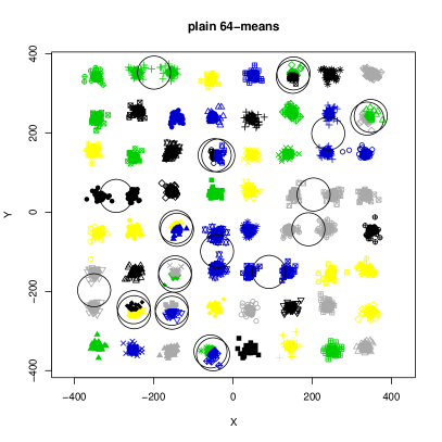
Figure 10: Worst misclustering errors $k$-means for the number of clusters $k$= 8 x 8 = 64 noise level= 30 %, cluster radius= 10 , cluster size= 96 , motion freedom of clusters= 10 , minimal distance between clusters: 5.83 *R

Some insights can be gained from the study of worst cases. One could have expected that the most problematic area would be the grid border. However, it does not seem to be so. Besides, glob-$k$-means seems to commit errors close to the grid center. So possibly, improvements of this algorithm should concentrate around the clusters close to the gravity center of all the data. $k$-means++seems to concentrate clusters without a hit in other area than those hit twice, even in the absence of noise. A review of the relSS in the tables shows that $k$-means can increase the SS even by a factor of 10. So its application in case of relatively clear cluster structure shall not be recommended.

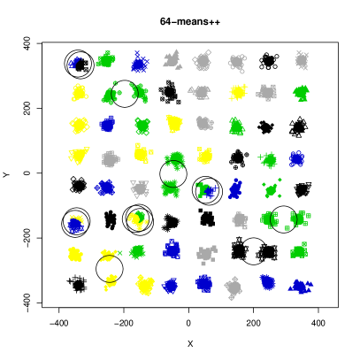
Figure 11: Worst misclustering errors $k$-means++ for the number of clusters $k$= 8 x 8 = 64 noise level= 30 %, cluster radius= 10 , cluster size= 96 , motion freedom of clusters= 10 , minimal distance between clusters: 5.83 *R

V Conclusions

In this research we were interesting in the question how well the popular family of algorithms, $k$-means, can handle well separated data under favourable conditions of coinciding global minimum of $k$-means cost function with the well-separation. We studied four popular algorithms ($k$-means, md-$k$-means, $k$-means++and glob-$k$-means) and our own algorithm $k$-means++B. For this purpose, we have identified the conditions under which well-separation coincides for sure with the $k$-means cost function minimum (see Theorems 1, 2. Given this theoretical result, series of experiments of algorithm performance with and without noise, with displacement and for varying cluster sizes were performed. It turned out that our algorithm exhibits the best performance while having acceptable executions time. A further research on properties of the new algorithm may be needed, in particular on the relationship between the boosting parameter and the noise levels. Also research on real datasets with artificially added noise may be insightful.

References

- [1] Margareta Ackerman and Sanjoy Dasgupta. Incremental clustering: The case for extra clusters. CoRR, abs/1406.6398, 2014.
- [2] A. Agrawal and H. Gupta. Global K-means (GKM) clustering algorithm: A survey. Intl’ J. of Computer Applications, 79(2):20–24, 2013. http://dx.doi.org/10.5120/13713-1472.
- [3] D. Arthur and S. Vassilvitskii. -means++: the advantages of careful seeding. In N. Bansal, K. Pruhs, and C. Stein, editors, Proc. of the Eighteenth Annual ACM-SIAM Symposium on Discrete Algorithms, SODA 2007, pages 1027–1035, New Orleans, Louisiana, USA, 7-9 Jan. 2007. SIAM.
- [4] Ardavan Ashabi, Shamsul Bin Sahibuddin, and Mehdi Salkhordeh Haghighi. The systematic review of k-means clustering algorithm. In ICNCC ’20: Proceedings of the 2020 9th International Conference on Networks, Communication and Computing,December 2020, page 13–18, 2020.
- [5] A.M. Bagirov, J. Ugon, and D. Webb. Fast modified global -means algorithm for incremental cluster construction. Pattern Recognition, 44(4):866–876, 2011. https://doi.org/10.1016/j.patcog.2010.10.018.
- [6] Vladimir Braverman, Adam Meyerson, Rafail Ostrovsky, Alan Roytman, Michael Shindler, and Brian Tagiku. Streaming k-means on well-clusterable data. In Proceedings of the Twenty-Second Annual ACM-SIAM Symposium on Discrete Algorithms, SODA ’11, page 26–40, USA, 2011. Society for Industrial and Applied Mathematics.
- [7] J. Xie et al. An efficient global k-means clustering algorithm. J. of Computers, 6(2):271–278, 2011. http://www.jcomputers.us/vol6/jcp0602-16.pdf.
- [8] G. Hannah Grace and Kalyani Desikan. Experimental estimation of number of clusters based on cluster quality. Journal of mathematics and computer science, 12:304–315, 2014.
- [9] T. Kanungo, D. M. Mount, N. S. Netanyahu, C. D. Piatko, R. Silverman, and A. Y. Wu. A local search approximation algorithm for k-means clustering. In Proceedings of the 18th Annual Symposium on Computational Geometry, Barcelona, Spain, June 5-7, 2002, pages 10–18, 2002.
- [10] M.A. Kłopotek and R.A. Kłopotek. On the discrepancy between kleinberg’s clustering axioms and k-means clustering algorithm behavior. Mach Learn, 112:2501–2553, 2023.
- [11] Mieczysław A. Kłopotek. On the existence of kernel function for kernel-trick of k-means in the light of gower theorem. Fundam. Inf., 168(1):25–43, jan 2019.
- [12] Mieczysław A. Kłopotek. On the consistency of k-means++ algorithm. Fundamenta Informaticae, 172(4):361–377, 2020.
- [13] Mieczysław A. Kłopotek. Clustering preserving transformation for k-means algorithm output. In Proc. ISMIS 2022, 03-05.10.2022, Cosenza, Italy, Lecture Notes in Computer Science book series (LNAI,volume 13515) Foundations of Intelligent Systems, page 315–322, 2022.
- [14] Mieczyslaw Alojzy Klopotek. An aposteriorical clusterability criterion for k-means++ and simplicity of clustering. SN Computer Science, 1, 2017.
- [15] Robert A. Kłopotek and Mieczysław A. Kłopotek. On probabilistic k-richness of the k-means algorithms. In Machine Learning, Optimization, and Data Science: 5th International Conference, LOD 2019, Siena, Italy, September 10–13, 2019, Proceedings, page 259–271, Berlin, Heidelberg, 2019. Springer-Verlag.
- [16] Robert Albert Klopotek, Mieczyslaw Alojzy Klopotek, and Slawomir T. Wierzchon. A feasible k-means kernel trick under non-euclidean feature space. International Journal of Applied Mathematics and Computer Science, 30:703 – 715, 2020.
- [17] Mieczysław Kłopotek, Slawomir Wierzchon, and Robert Kłopotek. k-means Cluster Shape Implications, pages 107–118. Springer Verlag, 05 2020.
- [18] Robert A. Kłopotek and Mieczysław A. Kłopotek. Solving inconsistencies of the perfect clustering concept. In Proc. of PP-RAI’2019 Congress, pages 273–276, 20129.
- [19] Yiwei Li. Generalization of k-means related algorithms. CoRR, abs/1903.10025, 2019.
- [20] A. Likas, N. Vlassis, and J.J. Verbeek. The global -means clustering algorithm. Pattern Recognition, 36(2):451–461, 2003. https://doi.org/10.1016/S0031-3203(02)00060-2.
- [21] Stuart P. Lloyd. Least squares quantization in pcm. IEEE Trans. Inf. Theory, 28(2):129–136, 1982.
- [22] Shuyu Miao, Lin Zheng, Jingjing Liu, , and Hong Jin. K-means clustering based feature consistency alignment for label-free model evaluation, 2023.
- [23] Neha B. Nikhare and Prakash S. Prasad. A review on inter-cluster and intra-cluster similarity using bisected fuzzy c-mean technique via outward statistical testing. In 2018 2nd International Conference on Inventive Systems and Control (ICISC), pages 215–217, 2018.
- [24] Rafail Ostrovsky, Yuval Rabani, Leonard J. Schulman, and Chaitanya Swamy. The effectiveness of lloyd-type methods for the k-means problem. J. ACM, 59(6), jan 2013.
- [25] M. Song and S. Rajasekaran. Fast algorithms for constant approximation k-means clustering. Trans. MLDM, 3(2):67–79, 2010.
- [26] Yi Wang, Jiahao Ma, Ning Gao, Qingsong Wen, Liang Sun, and Hongye Guo. Federated fuzzy k-means for privacy-preserving behavior analysis in smart grids. Applied Energy, 331:120396, 2023.
- [27] S.T. Wierzchoń and M.A. Kłopotek. Modern Clustering Algorithms, volume 34 of Studies in Big Data. Springer Verlag, 2018.