PePNet: A Periodicity-Perceived Workload Prediction Network Supporting Rare Occurrence of Heavy Workload

Abstract

Cloud providers can greatly benefit from accurate workload prediction. However, the workload of cloud servers is highly variable, with occasional heavy workload bursts. This makes workload prediction challenging. There are mainly two categories of workload prediction methods: statistical methods and neural-network-based ones. The former ones rely on strong mathematical assumptions and have reported low accuracy when predicting highly variable workload. The latter ones offer higher overall accuracy, yet they are vulnerable to data imbalance between heavy workload and common one. This impairs the prediction accuracy of neural network-based models on heavy workload. Either the overall inaccuracy of statistic methods or the heavy-workload inaccuracy of neural-network-based models can cause service level agreement violations. Thus, we propose PePNet to improve overall especially heavy workload prediction accuracy. It has two distinctive characteristics: (i) A Periodicity-Perceived Mechanism to detect the existence of periodicity and the length of one period automatically, without any priori knowledge. Furthermore, it fuses periodic information adaptively, which is suitable for periodic, lax periodic and aperiodic time series. (ii) An Achilles’ Heel Loss Function iteratively optimizing the most under-fitting part in predicting sequence for each step, which significantly improves the prediction accuracy of heavy load. Extensive experiments conducted on Alibaba2018, SMD dataset and Dinda’s dataset demonstrate that PePNet improves MAPE for overall workload by 20.0% on average, compared with state-of-the-art methods. Especially, PePNet improves MAPE for heavy workload by 23.9% on average.

I Introduction

Accurate workload prediction brings huge economic benefits to cloud providers [1] and many cloud frameworks make real-time adjustments based on the workload prediction results [2]. On the one hand, workload prediction provides meaningful insights to improve the utilization of cloud servers while ensuring quality of service (QoS) [3] [4]. On the other hand, it can also alarm the forthcoming uncommon heavy workload, thus helping to avoid service level agreement (SLA) violations.

TABLE I: Proportion of heavy workload.

Dataset	Heavy workload proportion
CPU usage of Alibaba’s dataset	15.73%
Memory usage of Alibaba’s dataset	12.89%
Workload of Dinda’s dataset [5]	11.15%

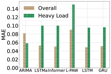
(a) The overall and heavy-workload prediction accuracy.

(b) Prediction of GRU on Alibaba2018.

Figure 1: Overall workload and heavy workload prediction accuracy.

However, the high variability of cloud-server workload [6] [7] makes workload prediction challenging. Statistical methods and neural-network-based models are two mainstream workload predicting methods. The former ones require the time series to satisfy strong mathematical assumptions and are uncompetitive when predicting highly variable workload [6]. For example, the classical statistic method, ARIMA [8], requires the time series to be stationary after difference and shows dissatisfied results when predicting highly variable workload [6]. The neural-network-based models are more suitable to predict highly variable workloads, but they are vulnerable to data imbalance between heavy workload and common one (the heavy workload is much more uncommon [9]). To demonstrate this, we present statistics of the heavy workload proportion of different datasets in Tab. I, where the heavy workload is defined as the workload greater than the average workload plus one standard deviation for each machine. It has also been proven that the data imbalance between heavy workload and common workload impairs the the former’s accuracy [10]. As an empirical example, Fig. 1 shows the overall prediction accuracy and heavy-workload prediction accuracy of some prevailing methods (ARIMA [8], LSTM with attention (LSTMa) [11], Informer [12], Learning based Prediction Algorithm for cloud workload (L-PAW) [6], LSTM and GRU) on Alibaba2018 dataset, where the heavy-workload predicted error is nearly twice as large as the overall predicted error. The inaccurate prediction will not only reduce the utilization of cloud servers but also bring SLA violations, as it provides wrong information to the scheduler.

To predict overall workload and heavy workload accurately, we propose a Periodic-Perceived Workload Prediction Network (PePNet), which supports the prediction of highly variable workload with the rarely-occurring heavy workload. PePNet mainly improves the prediction accuracy in two aspects: 1) using the periodically recurrent patterns to guide the workload prediction 2) using an Achilles’ Heel Loss Function, which pays more attention to the under-fitting part to offset the negative influence of data imbalance.

One challenge of utilizing the periodic information is that we have no priori knowledge of the periodicity (i.e., we neither know whether the time series is periodic nor do we know the length of its period). Besides, periodic and aperiodic time series are mixed and it is better to manipulate them with a unified architecture for convenience. Thus, we propose a Periodicity-Perceived Mechanism, which consists of Periodicity-Mining Module and Periodicity-Fusing Module. The Periodicity-Mining Module detects the periodicity and period length and the Periodicity-Fusing Module adaptively fuses the periodic information for periodic and aperiodic time series. One challenge of using is that Periodicity-Mining Module: one of its hyperparameter determinations depends on expert experience of workload. To solve this problem, we propose an automatic hyperparameter determination method for it based on statistical observations.

The Achilles’ Heel Loss Function specifically targets the upper bound of the prediction error, which enables PePNet to strengthen and improve the most vulnerable part of prediction. At each training step, the Achilles’ Heel Loss Function picks the most under-fitting part in a predicting sequence and minimizes its prediction error. The most under-fitting part shifts among different steps and each part in the predicting sequence is fitted alternatively. In this way, Achilles’ Heel Loss Function solves the under-fitting problem of heavy load and improves the heavy-load prediction accuracy as well as the overall prediction accuracy. The challenge for designing such a loss function is that the trivial operation of picking the most under-fitting part is non-differentiable during backpropagation. Thus, we propose a smooth operator for such an operation. Furthermore, we prove that such smooth operator can indefinitely approximate the trivial operation of picking the most under-fitting part.

The main contributions of our work are summarized as:

• designing a Periodicity-Perceived Mechanism, which mines and adaptively fuses the periodic information;

• proving an error bound of periodic information extracted by Periodicity-Fusing Module;

• providing an automatic hyperparameter determination method based on statistical observations;

• designing an Achilles’ Heel loss function by using a smooth operator to improve heavy-workload prediction accuracy and overall prediction accuracy;

• conducting extensive experiments on the Alibaba2018, SMD and Dinda’s datasets and demonstrating that PePNet improves the heavy-workload prediction accuracy (MAPE) up to 40.8% and 23.9% on average, while promoting overall prediction accuracy (MAPE) by 20.0% on average.

II Related Work

We first review existing methods for workload and time series prediction. Since PePNet uses periodic information, we also summarize related work for this topic.

II-A Workload and Time Series Prediction

Time series prediction aims to predict future time series based on the observed workload data. Based on its aims, workload prediction can be divided into: cloud resource allocation [13], autoscaling [14], etc. Based on users’ interests, the prediction can be divided into: the prediction of GPU workload [15], the prediction of CPU utilization [14], the prediction of virtual desktop infrastructure pool workload [16], the prediction of disk healthy states [17], workload prediction framework [18], etc.

As workload prediction is a branch of time series prediction, it is necessary to review the development of time series prediction. There are several research directions. To improve the prediction accuracy of dynamic real-world time series, researchers propose some traditional recurrent neural network [19] [20] to replace classical statistic methods [8] [21] [22]. To improve the model memory of long input sequences, researchers propose models combining recurrent neural networks and attention mechanism [11] [23]. To improve the prediction accuracy of a long sequence, researchers propose models based on variants of transformer [24] [25] [12] and auto-encoder [6]. To make use of the relevance among different channels in multi-variant time series, researchers propose models combining GNN or CNN with time series manipulating networks [26] [27]. Another research direction is improving the robustness of deep networks dealing with time series. The robustness includes five implications: the robustness for missing data, the robustness for the malicious or limited labels, the generalization of the trained model, the robustness toward noise in time series, and the robustness for the irregular data sampling period. For example, Belkhouja et al. propose a Robust Training for Time-Series (ROTS) to improve deep neural network robustness for generalization and noise [28]; Tan et al. propose Dual-Attention Time-Aware Gated Recurrent Unit (DATA-GRU) to manipulate time series sampled in an irregular period [29]; Zhang et al. propose Multivariate Time Series Classification with Attentional Prototypical Network (TapNet) to deal with time series with limited labels [30]; Tang et al. propose network modeling local and global temporal dynamics (LGnet) to deal with a data-missing problem in time series [31]; Luo et al. propose $E^{2}GAN$, which uses adversarial learning to deal with data missing problem [32]; Yao et al. propose Spatial-Temporal Dynamic Network (STDN) to deal with lax-strict periodicity caused by noise [33]; Luo et al. propose Uncertainty-Aware Heuristic Search (UAHS) to deal with uncertain prediction error caused by noise [18]. But none of these methods focus on dealing with the prediction accuracy of heavy workload.

II-B Periodicity Information Extraction

In the field of traffic forecasting, there is also significant periodicity and we summarize some recent popular methods below. There are several mechanisms to fuse periodic information. For example, Guo et al. propose a novel attention-based spatial-temporal graph convolution network [34]; Lv et al. use a fully-connected layer and take advantage of both CNN and RNN to deal with periodic time series [26]; Chen et al. propose Hop Res-RGNN to deal with periodic patterns [35]. But these methods do not consider the lax periodicity of time series. Yao et al. propose an attention mechanism to tackle periodic shift [33]. These studies use the priori knowledge of the daily and weekly periodicity of traffic loads. However, in the scenario of service load prediction, there is usually no priori knowledge about the periodicity. Besides, the periodicity of the time series in these studies is fixed, while the periodicity of workload for different machines are variable.

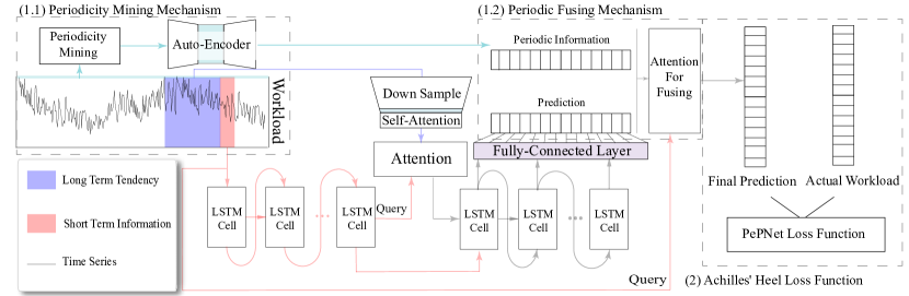
Figure 2: The overview of PePNet.

III Methodology

III-A Overview of PePNet

PePNet is based on an encoder-decoder [36] architecture and fuses three kinds of information from rough data: the long-term tendency information, the short-term dependent information and the periodic information. Besides, the whole model is trained by an Achilles’ Heel Loss Function to offset the negative impact of data imbalance. The overview of PePNet is shown in Fig. 2.

The input of data $X$ is divided into three parts, which are denoted by $X^{enc}_{short}\in\mathbb{R}^{I\times d}$, $X^{enc}_{long}\in\mathbb{R}^{M\times d}$, $X_{period}\in\mathbb{R}^{P\times d}$ respectively. The $d$ is the dimension of the feature at each time slot and $I,M$ and $P$ respectively stand for the length of short-term dependent information, long-term tendency information and periodic information, respectively. The data division is shown in Fig. 3(a): $Y$ is the ground truth value of predicting workload; $X^{enc}_{short}$ is the nearest workload time series before the predicting part and shows high relevance to predicting workload; $X^{enc}_{long}$ is a bit longer workload time series before $X^{enc}_{short}$ and reflects the long term tendency in workload variation; $X_{period}$ is the first period of workload for each machine; The $y_{period}$ is the workload sequence corresponding to $Y$ in the period of $X_{period}$. The extracting process of $X_{period}$ and $y_{period}$ is illustrated in section III-B1. We use $X^{enc}_{long,i}$ and $X^{enc}_{short,i}$ to denote the $i$-th time slot’s workload in $X^{enc}_{long}$ and $X^{enc}_{short}$ respectively.

These three kinds of information bring different effects for workload prediction. The short-term dependent information $X^{enc}_{short}$ is highly related to the predicting sequence, as the customers’ behaviors are continuous and the workload is similar in a short time slot. The long-term tendency information denotes the forthcoming heavy load, as the heavy load is more likely to happen in ascending tendency. This tendency information is usually masked by noises in the short term and has to be extracted from long-term time series. As shown in Fig. 3(b), we pick a small segment of the workload from a long-term-ascending sequence. Though the long-term ascending tendency it is, the short-term workload just fluctuates around a stable value and does not show any increasing tendency. The periodic information provides the recurrent patterns in history and promotes both overall prediction accuracy and heavy-load prediction accuracy.

According to the different properties of these three kinds of information, PePNet uses different modules to deal with them in the encoder. PePNet uses an LSTM to capture short-term dependent information from $X^{enc}_{short}$ and uses Periodicity-Mining Module to detect and extract periodic information from $X_{period}$. As for long-term tendency information, PePNet firstly downsamples $X^{enc}_{long}$, as it helps to improve the processing efficiency as well as maintain and magnify the trend information of time series. Then, PePNet uses self-attention to manipulate the down-sampled sequence. In this way, PePNet reduces the forgetting effect [12] in long sequence processing. The processes of extracting short-term, long-term and periodic information are shown in Eq.1-3. In the function $LSTM(x,h,c)$, $x$, $h$, $c$ respectively stand for the input of LSTM, the hidden state and the cell state[37]. In function $Attention(q,k,v)$, $q$, $k$, $v$ respectively stand for the query, key and value[38].

$$\overline{X}^{enc}_{short,i+1},h_{i+1},c_{i+1}=LSTM(X^{enc}_{short,i},h_{i},c_{i})$$ (1)

$$y_{period},X_{period}=PeriodicityMining(X,X^{enc}_{short})$$ (2)

$$\overline{X}^{enc}_{long}=Downsample(Attention(X^{enc}_{long},X^{enc}_{long},X^{enc}_{long}))$$ (3)

In the decoder, PePNet uses LSTM to generate $\hat{y}\in\mathbb{R}^{J\times d}$, where $J$ stands for the predicting length. After that, PePNet uses Periodicity-Fusing Module to estimate the reliability of $\hat{y}$ and fuses it with $y_{period}$ according to their reliability. By then, the Periodicity-Fusing Module generates the final prediction $y$. The process of decoder is shown in Eq.4-7, where $W_{h},W_{c}$ are both model parameters. The symbol $\oplus$ stands for concatenation.

$$\hat{y}_{j+1},h_{j+1},c_{j+1}=LSTM(\hat{y}_{j},h_{j+\frac{1}{2}},c_{j+\frac{1}{2}})$$ (4)

$$h_{j+\frac{1}{2}}=W_{h}\cdot(Attention(h_{j},\overline{X}^{enc}_{long},\overline{X}^{enc}_{long})\oplus h_{j})$$ (5)

$$c_{j+\frac{1}{2}}=W_{c}\cdot(Attention(c_{j},\overline{X}^{enc}_{long},\overline{X}^{enc}_{long})\oplus c_{j})$$ (6)

$$y=PeriodicityFusing(X^{enc}_{short},y_{period},\hat{y})$$ (7)

When training the model, the imbalance between heavy load and normal workload usually leads to unsatisfactory accuracy of heavy load prediction. Thus, we propose an Achilles’ Heel Loss function, which aims to minimize the upper bound of prediction error. At each step, Achilles’ Heel Loss Function iteratively optimizes the most under-fitting part for this step, in order to improve the prediction accuracy of the heavy load when keeping the overall prediction accurate. It is named after Achilles’ Heel as it focuses on the most vulnerable portion along the predicting sequence. Thus, the prediction accuracy of the heavy load becomes more accurate, when keeping the overall prediction accurate. One challenge for minimizing the upper bound is that the operation of picking the upper bound is usually non-differentiable. Thus, we propose a smooth operator instead of hard segmentation. It is proved that the smooth operator can be infinitely close to the operation of picking the upper bound.

The most distinctive characters of PePNet lie in: 1) it is equipped with the Periodicity-Perceived Mechanism to mine the periodicity (Periodicity-Mining Module) and adaptively fuse the periodic information (Periodicity-Fusing Module); 2) it theoretically proves the error boundary of extracted periodic information; 3) it uses an automatic hyperparameter determination method for Periodicity-Mining Module; 4) it uses an Achilles’ Heel Loss Function to mitigate the negative effect of data imbalance on model performance.

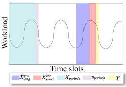
(a) The input data division.

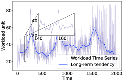
(b) The long term tendency information.

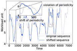
(c) Local periodicity violation in lax periodic series.

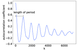
(d) Autocorrelation coefficient for periodic sequence.

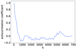
(e) Autocorrelation coefficient for aperiodic sequence.

(f) The method of computing periodic information.

Figure 3: Illustrations for periodicity-perceived mechanism.

III-B Periodicity-Perceived Mechanism

Periodic information can effectively improve the overall prediction accuracy as well as the heavy workload prediction accuracy. It consists of Periodicity-Mining Module and Periodicity-Fusing Module.

There are three main challenges to fuse periodic information. (1) We have no priori knowledge about the periodicity of workload for different machines, which calls for the Periodicity-Mining Module to detect the existence of periodicity and the length of one period. (2) The periodicity for different machines is variable (i.e., strict periodic, lax periodic, aperiodic), which calls for an adaptive Periodicity-Fusing Module. (3) It is hard to fuse the periodic information in lax periodic series, because lax periodic series are sometimes periodic and sometimes not. In Fig. 3(c), we overlap a series shifted one period ahead and the original series. As Fig. 3(c) shows, there are mainly two obstacles to fuse periodic information in lax periodic series: periodic shift and local periodicity violation. The former one can be solved by dynamic matching which is depicted in section Periodicity-Mining Module. The latter one is caused by noise and external events. Therefore, we filter out the noise in periodic information in Periodicity-Mining Module and evaluate the reliability of periodic information in the Periodicity-Fusing Module.

III-B1 Periodicity-Mining Module

PePNet calculates the time series autocorrelation coefficient $\rho_{k}$ for each machine as shown in Eq.8, which represents the linear correlation among all workloads with interval $k$ (i.e., linear correlation between $X_{t}$ and $X_{t-k}$, for every $t\in\{t\in\mathbb{N}^{+}|t<sequence\ length\}$, $X_{t}$ stands for the workload at $t$-th time slot). As shown in Fig. 3(d), when the workload is periodic, the autocorrelation coefficient rises to a large value again after the first decline, which represents a high hop relevance of workload. While the sequence is aperiodic, the autocorrelation coefficients are shown in Fig. 3(e), which have a distinct pattern. Therefore, PePNet sets a hyperparameter $\mathcal{T}$ and judges whether a time series is periodic by detecting whether the autocorrelation coefficient crosses over $\mathcal{T}$ again. The value of $\mathcal{T}$ denotes the acceptable range of periodicity strictness.

$$\rho_{k}=\frac{cov(X_{t-k},X_{t})}{\sqrt{cov(X_{t},X_{t})cov(X_{t-k},X_{t-k})}}$$ (8)

The position of the first peak in autocorrelation coefficients of periodic sequence strikes the highest hop relevance and denotes the length of one period. We illustrate it in Fig. 3(d). The reason why the autocorrelation coefficient shows such a pattern is that the user behavior is continuous in time, so the autocorrelation coefficients of small $k$ are large. As the time interval $k$ increases, the relevance drops down. But when the time interval $k$ reaches around the integer multiple of period length, the workload at the two moments $X_{t}$ and $X_{t-k}$ shows a high linear correlation again.

Based on these observations, as shown in Algorithm 1, PePNet traverses the value of $k$ from small to large. If PePNet finds the smallest $k$ that makes the autocorrelation coefficient $\rho_{k}$ satisfy the conditions: $\rho_{k}>\rho_{k-1},\rho_{k}>\rho_{k+1}$ and $\rho_{k}>\mathcal{T}$, the time series is periodic and the length of one period is $k$. Otherwise, the time series is aperiodic. We cut out the first period of the machines whose workloads are periodic in the training set as a periodic information knowledge base, which is denoted by $X_{period}$. To solve the issue of period shift, PePNet uses a dynamic matching. If the workload is periodic, PePNet finds the sequence $\{X_{t_{a}},\ldots,X_{t_{a}+I-1}\}$ in $X_{period}$, whose distance from $X^{enc}_{short}$ is the smallest. The distance can be computed either by Mean Square Error (MSE) or by Dynamic Time Warping (DTW). Then, PePNet sets $y_{period}=\{X_{t_{a}+I},\ldots,X_{t_{a}+I+J}\}$. Otherwise, $\{-1,-1,\ldots,-1\}$ is set to $y_{period}$. Such a process is illustrated in Fig. 3(f).

Data: Workload time series $X$, Short-term dependent information $X^{enc}_{short}$

Result: The periodic information for prediction $y_{period}$, The periodic knowledge base $X_{period}$

1 $k\leftarrow-1$;

2 while $k<length(X)$ do

3      $k\leftarrow k+1$;

4       Compute $\rho_{k}$;

5       if $\rho_{k}>\rho_{k-1}\ and\ \rho_{k}>\rho_{k+1}\ and\ \rho_{k}>\mathcal{T}$ then

6            Period length=k ;

7             FoundPeriodLength=True ;

8             break ;

9       end if

10      

11 end while

12if FoundPeriodLength then

13       $X_{period}=X[:Period\ length]$;

14       $y_{pos}=\arg\min_{t_{a}}Distance(X[t_{a}:t_{a}+I],X^{enc}_{short})$;

15       $y_{period}=X[y_{pos}:y_{pos}+I]$;

16      

17 end if

18else

19       $X_{period}=-1$;

20       $y_{period}=[-1,\ldots,-1]$;

21      

22 end if

Algorithm 1 Periodicity-Mining Module

Error estimation. We use $E[(X_{t-k}-X_{t})^{2}]$ to measure the quality of periodic length $k$ found by the Periodicity-Mining Module. We have the following result.

Theorem 1. When using Algorithm 1, $E[(X_{t-k}-X_{t})^{2}]$ is upper bounded by $(\Delta\sigma)^{2}+(\Delta\mu)^{2}+2(1-\mathcal{T})\sigma_{t-k}\sigma_{t}$, where $\sigma_{t-k},\sigma_{t},\mu_{t-k},\mu_{t}$ are the standard deviation and expectation at $t-k$ and $t$ time slots respectively. The $\Delta\sigma$ and $\Delta\mu$ are $\sigma_{t-k}-\sigma{t}$ and $\mu_{t-k}-\mu_{t}$ respectively. Furthermore, when the time series is stationary, $E[(X_{t-k}-X_{t})^{2}]$ is upper bounded by $2(1-\mathcal{T})\sigma_{t-k}\sigma_{t}$, where $\sigma$ is the standard deviation of the time series.

Proof of Theorem 1. According to algorithm 1, when PePNet finds $k$, Eq.9-10 holds, where $a_{i}=X_{i}-\mu_{i}$, $\tilde{t}=t-k$. $E[(X_{\tilde{t}}-X_{t})^{2}]$ can be transformed to Eq.11. Then, we substitute Eq.10 into Eq.11 and obtain Eq.12. The Eq.12 can be further reduced into Eq.13 and the first part of Theorem 1 is proven. When the time series is stationary, $\Delta\sigma^{2}$ and $\Delta\mu^{2}$ are zero. Then the upper bound can be reduced to $2(1-\mathcal{T})\sigma_{t-k}\sigma_{t}$.

$$\frac{E[a_{\tilde{t}}a_{t}]}{\sigma_{\tilde{t}}\sigma_{t}}>\mathcal{T}$$ (9)

$$E[a_{\tilde{t}}a_{t}]>\mathcal{T}*\sigma_{\tilde{t}}\sigma_{t}$$ (10)

$$E[(X_{\tilde{t}}-X_{t})^{2}]=E[a_{\tilde{t}}^{2}+a_{t}^{2}-2a_{\tilde{t}}a_{t}+2\Delta\mu\Delta a+\Delta\mu^{2}]$$ (11)

$$E[(X_{\tilde{t}}-X_{t})^{2}]<E[a_{\tilde{t}}^{2}]+E[a_{t}^{2}]-2*\mathcal{T}\sqrt{E[a_{\tilde{t}}^{2}]E[a_{t}^{2}]}+\Delta\mu^{2}$$ (12)

$$E[(X_{\tilde{t}}-X_{t})^{2}]<\Delta\sigma^{2}+\Delta\mu^{2}+2(1-\mathcal{T})\sigma_{\tilde{t}}\sigma_{t}$$ (13)

Taking a further look at the upper bound, the first and second items of the upper bound are constants. Thus, the value of error depends on the last item, which is determined by the value of $\mathcal{T}$. Considering that the $\mathcal{T}$ is less than or equal to one, the closer the $\mathcal{T}$ is to one, the smaller the error is. However, most of the time series are lax periodic in reality. Setting the $\mathcal{T}$ as 1 may miss many lax periodic time series. Thus, there is a tradeoff between improving the accuracy of periodic length and finding all the periodic time series (including lax periodic time series).

Considering the tradeoff may make it challenging to choose a proper value of $\mathcal{T}$, we provide an automatic setting method for $\mathcal{T}$ based on statistical observations. For finer tuning, this method provides a searching range for $\mathcal{P}$. The hyperparameter $\mathcal{P}$ is a threshold setting for the first peak of the autocorrelation coefficient. Thus, we look into the distributions of the first peak value. Taking Alibaba2018-CPU as an example, we take 75 machines in it and plot a histogram of first-peak value in Fig. 4. There are two properties of the distribution: clustered and following Gaussian Distribution for each cluster. We use Gaussian Mixture Model (GMM) algorithm to fit the mixed Gaussian distribution of its first peak values and plot the Gaussian distributed curve on the histogram in Fig. 4. The parameter for this GMM is given in Tab. II. Different clusters have different degrees of periodicity. The higher the expectation of the cluster is, the stricter its periodicity is. To guarantee the quality of the periodicity the Periodicity-Mining Module detects, it picks workload in the cluster with the highest expected value as periodic and filters the others. Let $\mu$ and $\sigma$ denote the expectation and standard deviation of the cluster with the highest expectation. In industrial applications, $\mu-\sigma$ can be directly used as the $\mathcal{P}$ to save the labor costs, as the probability that the first peak is greater than $\mu-\sigma$ in this cluster is 84.2% according to Gaussian distribution. For finer tuning, the $mathcal{P}$ can be explored between $\mu-\sigma$ and $\mu+\sigma$.

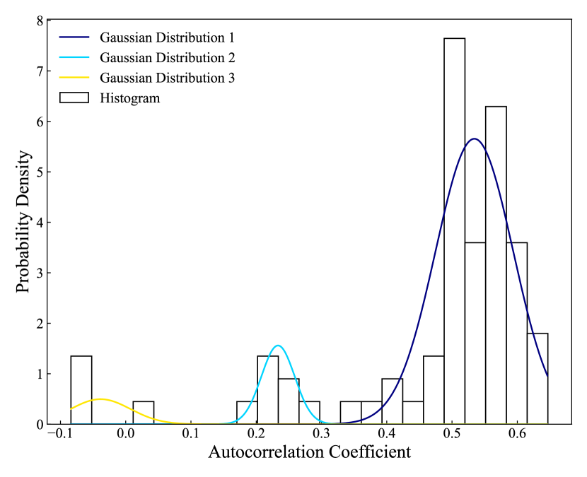
Figure 4: Histogram of values for the first peak of the autocorrelation coefficient.

TABLE II: Parameters of Gaussian distribution.

	weight	expectation	standard deviation
Gaussian distribution 1	0.84	0.53	0.06
Gaussian distribution 2	0.10	0.23	0.03
Gaussian distribution 3	0.06	-0.04	0.05

III-B2 Periodicity-Fusing Module

To filter out the random noise in the periodic information, PePNet firstly uses an auto-encoder [39]. To solve the problem of variable periodicity for different machines and the problem of local periodicity violation, PePNet uses an attention mechanism to evaluate the reliability of periodic information. The final prediction $y$ is given in Eq.14-15.

$$y_{period}^{{}^{\prime}}=Autoencoder(y_{period})$$ (14)

$$y=Attention(X^{enc}_{short},(\hat{y},y_{period}^{{}^{\prime}}),(\hat{y},y_{period}^{{}^{\prime}}))$$ (15)

III-C Achilles’ Heel Loss Function

As mentioned before, heavy load rarely occurs, which leads to poor performance of heavy load prediction due to data imbalance. To solve this problem, PePNet minimizes the worst case in a predicting sequence for each step. When iteratively training the model, PePNet optimizes the worst case in one step and in the next step the worst case may occur at another place. In this way, Achilles’ Heel Loss Function optimizes the most under-fitting part at each training step and effectively improves the accuracy of heavy load. A native idea is to optimize the prediction with the highest error in each predicting sequence, as shown in Eq.16. In Eq.16, $T$ equals $\{t_{1},\ldots,t_{1+J}\}$, which are the time slots of a forecasting sequence. $y_{t}$ denotes the predicted workload at time $t$ (the prediction length for one sample should be at least 2), and $Y_{t}$ denotes the ground-truth workload at time $t$.

$$l(Y,y)=\max_{t\in T}(y_{t}-Y_{t})^{2}$$ (16)

However, the function in Eq.16 is not smooth and cannot be derived for backpropagation. Inspired by [40], we propose a smooth max operator in Eq.17, where $\gamma$ is a hyperparameter and $A_{i}$ can be any variable. Then, the loss function in Eq.16 can be transformed into Eq.18.

$$\max(A_{1},A_{2},\ldots,A_{N})=\gamma\log(\sum^{N}_{i}exp(\frac{A_{i}}{\gamma})),\gamma>0$$ (17)

$$l(Y,y)=\gamma\log(\sum^{T}_{t}exp(\frac{(y_{t}-Y_{t})^{2}}{\gamma})),\gamma>0$$ (18)

Let us take a further look at Eq.18. It actually distributes more weight to the gradient for higher prediction error when back propagating. This aspect is obvious by deriving Eq.18, as shown in Eq.19, where $\alpha_{t}=\frac{exp{\frac{(y_{t}(\mathcal{P})-Y_{t})^{2}}{\gamma}}}{\sum_{t=1}^{T}\exp{\frac{(y_{t}(\mathcal{P})-Y_{t})^{2}}{\gamma}}}$, $\mathcal{P}$ stands for the parameters of PePNet. $\alpha_{t}$ is actually a normalized weight, whose value depends on the prediction error at time slot $t$. $\gamma$ is a scale factor. When $\gamma$ is large, the difference in prediction errors across time slots is narrowed and the weights are relatively uniform for each time slot. When the $\gamma$ is small, the difference in prediction errors across time slots is amplified and the weights become polarized. To visually demonstrate this point, we plot the value of $\alpha_{t}$ for different combinations of $\gamma$ and prediction error $y_{t}-Y_{t}$ in Fig. 5. In Fig. 5, each row shows the value of $\alpha_{t}$ for a set of prediction error $\{y_{t}-Y_{t}|0\leq t\leq 9\}$, when specifying the $\gamma$. As Fig. 5 shown, for a specific $\gamma$, the larger the prediction error is, the bigger the $\alpha_{t}$ is. Besides, for a specific prediction error in a specific error set, the smaller the $\gamma$ is, the bigger the $\alpha_{t}$ is. When $\gamma$ is set to 0.1, $\alpha_{t}$ for the largest prediction error in this row approximates 1.

$$\frac{\partial l(Y,y)}{\partial\mathcal{P}}=\sum_{t=1}^{T}(\alpha_{t}\cdot\frac{\partial{(y_{t}(\mathcal{P})-Y_{t})^{2}}}{\partial\mathcal{P}})$$ (19)

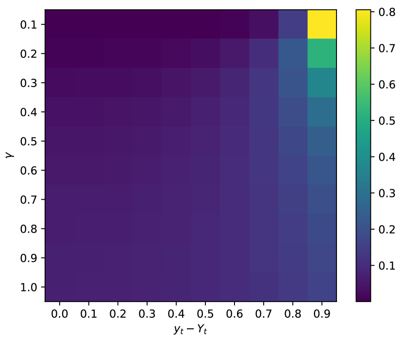
Figure 5: How the value of $\gamma$ impacts the distribution of gradient weights.

To theoretically prove this tendency, let us look into the extreme situation when the $\gamma$ is infinitely close to 0. We have the following result that implies when $\gamma$ indefinitely approximates 0, only the gradient for maximum prediction error is assigned a weight of 1, while others are assigned a weight of 0.

Theorem 2. As the $\gamma$ is infinitely close to 0, the gradient of the loss function infinitely approximates Eq.20. The $t^{*}=\mathop{\arg\max}_{t}(y_{t}-Y_{t})^{2}$ and the $g(t^{*},\mathcal{P})=(y[t^{*}]-Y[t^{*}])^{2}$.

$$\frac{\partial l(Y,y)}{\partial\mathcal{P}}=\frac{\partial g(t^{*},\mathcal{P})}{\partial\mathcal{P}}$$ (20)

Proof of Theorem 2. The derivation of $l(Y,y)$ is shown in Eq.21. Then, both the numerator and dominator on the right-hand side are divided by $\exp(\frac{g(t^{*},\mathcal{P})}{\gamma})$ simultaneously and the first step of Eq.22 is obtained. The $g(t^{*},\mathcal{P})$ is surely bigger than $g(t,\mathcal{P}),\forall t\neq t^{*}$, as the definition of $t^{*}$ suggests. Thus, $g(t,\mathcal{P})-g(t^{*},\mathcal{P})<0,\forall t\neq t^{*}$. When the $\gamma(\gamma>0)$ infinitely approaches zero, $exp(\frac{g(t,\mathcal{P})-g(t^{*},\mathcal{P})}{\gamma})$ will also infinitely approaches zero. In this way, the second step of Eq.22 is obtained.

$$\frac{\partial l(Y,y)}{\partial\mathcal{P}}=\frac{\sum_{t}^{T}[exp(\frac{g(t,\mathcal{P})}{\gamma})\frac{\partial g(t,\mathcal{P})}{\partial\mathcal{P}}]}{\sum_{t}^{T}exp(\frac{g(t,\mathcal{P})}{\gamma})}$$ (21)

$$\mathop{\lim}_{\gamma\rightarrow 0}\frac{\partial l(Y,y)}{\partial\mathcal{P}}$$ (22)

$$=\mathop{\lim}_{\gamma\rightarrow 0}\frac{\frac{\partial g(t^{*},\mathcal{P})}{\partial\mathcal{P}}+\sum_{t,t\neq t^{*}}^{T}[exp(\frac{g(t,\mathcal{P})-g(t^{*},\mathcal{P})}{\gamma})\frac{\partial g(t,\mathcal{P})}{\partial\mathcal{P}}]}{1+\sum_{t,t\neq t^{*}}^{T}exp(\frac{g(t,\mathcal{P})-g(t^{*},\mathcal{P})}{\gamma})}$$

$$=\frac{\partial g(t^{*},\mathcal{P})}{\partial\mathcal{P}}$$

IV Experiment

In this section, we conduct extensive experiments to validate the following findings:

• PePNet improves the accuracy of heavy-workload prediction as well as improving the overall prediction accuracy with respect to the state of the art.

• PePNet only introduces slight time overhead for training and inference.

• PePNet is insensitive to hyperparameters and has high robustness robustness.

• Each mechanism in PePNet is proven to play an important role by using ablation experiments.

• Due to its adaptability for periodicity, when the time series is aperiodic, PePNet still works well.

TABLE III: Basic hyperparameters of PePNet.

Hyperparameter	Value
Batchsize of Alibaba2018-CPU	100
Learning rate of Alibaba2018	0.001
Learnig rate of Dinda’s dataset	0.0005
Learning rate of SMD	0.01
$\mathcal{T}$ of Alibaba2018-Mem	0.2
$\mathcal{T}$ of others	0.5
$\gamma$	$\mathop{\lim}_{\gamma\rightarrow 0}$
Number of layers of LSTM	2
Input length of Alibaba2018 for short-term information	50
Input length of Alibaba2018 for long-term information	100
Input length of Dinda’s dataset for short-term information	30
Input length of Dinda’s dataset for long-term information	80
Input length of SMD for short-term information	50
Input length of SMD for long-term information	100
Hidden layer size of LSTM	80
Predicted length	2
Init downsampling step size	20
Number of layers of auto-encoder	1
Number of layers of auto-decoder	1
Output size of auto-encoder	1
Sliding window length for downsampling	100

IV-A Experiment Setup

Hyperparameters. We summarize the most important hyperparameters of PePNet in Tab. III.

Baseline Methods. We compare PePNet with the state-of-art time series predicting method and popular workload predicting models and the variants of PePNet.

• Autoformer (Autof) [24]: Autoformer is a novel decomposition architecture with an Auto-Correlation mechanism. It breaks the pre-processing convention of series decomposition and renovating it as a basic inner block of deep models. Further, Autoformer also has an Auto-Correlation mechanism based on the series periodicity.

• LSTM with attention mehcanism (LSTMa) [11]: The approach extracts the sequential and contextual features of the historical workload data by an encoder network and integrates an attention mechanism into the decoder network.

• Informer (Inf) [12]: The method uses a ProbSparse attention mechanism and a halving cascading layer to extract the input information and use a generative style decoder to predict. Informer is one of the most recognized methods of time series prediction in recent years.

• L-PAW [6]: The method integrates top-sparse auto-encoder (TSA) and gated recurrent unit (GRU) block into RNN to achieve the adaptive and accurate prediction for highly-variable workloads. L-PAW is a model specifically designed for workload prediction and is also widely used.

• LSTM [37]: A classic time series processing model, which uses the hidden state to store long sequences of information.

• GRU [36]: A variant of the LSTM which modifies the forget gate structure in LSTM to make the model simpler.

• Reformer (Ref) [25]: Reformer introduces two techniques to improve the efficiency of Transformers. Firstly, it replaces dot-product attention with one that uses locality-sensitive hashing. Secondly, it uses reversible residual layers instead of standard residuals to reduce the memory consumption of the model. It is a widely recognized method in time series prediction.

• Fedformer (Fedf) [41]: Fedformer combines Transformer with a seasonal-trend decomposition method, in which the decomposition method captures the global profile of time series while Transformers capture more detailed structures. Fedformer is an effective and novel method in time series prediction.

• Variants of PePNet: These approaches are introduced for ablation study. We use PePNet^- to denote the PePNet that removes the Periodicity-Perceived Mechanism. We use PePNet^† to denote the PePNet that uses MSE as a loss function. We use PePNet^‡ to denote the PePNet that both removes the Periodicity-Perceived Mechanism and does not use the Achilles’ Heel loss function.

TABLE IV: The overall and heavy-workload prediction accuracy on three datasets. The MSE in the table are multiplied by 1000.

			LSTM	LSTMa	GRU	Inf	L-PAW	Ref	Autof	Fedf	PePNet-	PePNet†	PePNet‡	PePNet
		MAPE	0.093	0.117	0.108	0.100	0.102	0.104	0.211	0.110	0.089	0.087	0.116	0.076
	Overall	MSE	5.515	8.233	9.516	4.865	10.960	8.950	37.636	9.211	5.773	6.146	6.847	3.697
Dinda’s		MAE	0.048	0.071	0.070	0.041	0.078	0.053	0.149	0.057	0.046	0.049	0.059	0.029
Dataset		MAPE	0.051	0.079	0.094	0.030	0.046	0.040	0.079	0.032	0.035	0.043	0.058	0.018
	Heavy-Workload	MSE	12.260	17.925	24.191	6.837	15.853	9.202	23.817	8.729	5.635	7.325	13.274	6.124
		MAE	0.068	0.104	0.123	0.040	0.058	0.051	0.097	0.041	0.046	0.057	0.076	0.025
		MAPE	0.179	0.238	0.287	0.237	0.296	0.278	0.488	0.290	0.207	0.191	0.161	0.154
	Overall	MSE	3.434	3.627	3.889	3.282	3.909	4.950	8.021	2.350	3.144	2.974	3.101	1.757
SMD		MAE	0.019	0.023	0.025	0.022	0.025	0.028	0.046	0.023	0.020	0.019	0.018	0.014
Dataset		MAPE	0.150	0.163	0.154	0.166	0.154	0.316	0.367	0.157	0.138	0.129	0.158	0.112
	Heavy-Workload	MSE	10.437	10.622	11.945	11.024	11.912	17.587	27.465	5.531	10.941	9.751	10.399	6.729
		MAE	0.037	0.045	0.046	0.041	0.046	0.068	0.095	0.034	0.042	0.038	0.040	0.033
		MAPE	0.039	0.095	0.049	0.058	0.157	0.086	0.037	0.025	0.050	0.027	0.126	0.016
	Overall	MSE	0.375	0.489	0.462	0.408	12.721	0.880	1.173	0.510	0.359	0.341	0.975	0.323
Alibaba		MAE	0.014	0.017	0.015	0.015	0.058	0.023	0.026	0.016	0.014	0.013	0.024	0.013
Memory		MAPE	0.023	0.023	0.027	0.027	0.039	0.022	0.032	0.030	0.019	0.019	0.030	0.019
	Heavy-Workload	MSE	0.706	0.673	0.860	0.919	2.420	0.695	1.418	1.182	0.566	0.542	1.114	0.509
		MAE	0.021	0.020	0.023	0.024	0.032	0.019	0.029	0.027	0.018	0.018	0.028	0.017
		MAPE	0.173	0.215	0.181	0.165	0.272	0.190	0.258	0.158	0.139	0.158	0.150	0.142
	Overall	MSE	4.647	4.996	4.753	4.809	12.638	6.097	9.954	6.204	4.786	4.812	4.784	4.758
Alibaba		MAE	0.049	0.053	0.051	0.050	0.090	0.060	0.073	0.056	0.050	0.051	0.050	0.049
CPU		MAPE	0.195	0.237	0.194	0.193	0.343	0.247	0.381	0.252	0.178	0.177	0.182	0.143
	Heavy-Workload	MSE	16.767	17.548	16.228	17.742	29.493	18.848	32.271	22.226	16.594	16.321	16.405	11.634
		MAE	0.095	0.100	0.096	0.100	0.150	0.105	0.145	0.115	0.097	0.095	0.095	0.082

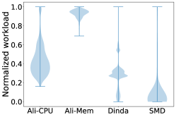
(a) Data distribution of different datasets

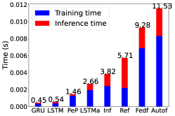
(b) Time overhead of different methods

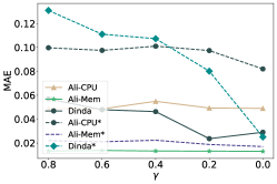
(c) MAE of PePNet with different $\gamma$

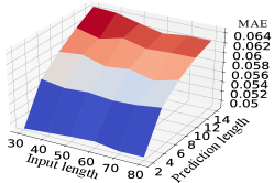
(d) Overall MAE of PePNet on Alibaba2018-CPU

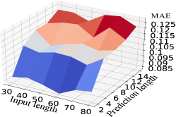
(e) Heavy-workload MAE of PePNet on Alibaba2018-CPU

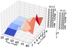
(f) Overall MAE of PePNet on Alibaba2018-Memory

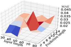
(g) Heavy-workload MAE of PePNet on Alibaba2018-Memory

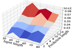
(h) Overall MAE of PePNet on Dinda’s dataset

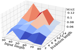
(i) Heavy-workload MAE of PePNet on Dinda’s dataset

Figure 6: (a) The value of the y-axis is the original workload divided by the maximum workload of its machine. The wider the width of the violin in the figure is, the more workloads are distributed near this value. (b) The figure shows the average consuming time of one forward propagation and backpropagation for one sample. The labels on the histogram are 1000 times of the actual value. Besides, we use the shorthand of Informer, Autoformer and Reformer in the xticks. (c) The figure shows the overall and heavy-workload MAE of PePNet for different $\gamma$ on all the three datasets. In the legend, we use dataset name* to represent the heavy-workload MAE on the specific dataset, while using dataset name to represent the overall MAE on the dataset. (d)-(i) These figures show overall and heavy-workload MAE of PePNet on different datasets with different combination of the length of $X_{in}$ and $p$.

Datasets. We perform experiments on three public datasets: Alibaba’s cluster trace v2018, Dinda’s dataset [5] and Server Machine Dataset (SMD) [42]. These datasets are collected by different organizations with different system configurations. Their use can help to verify the generalization of PePNet. We plot the data distribution of different datasets in Fig. 6(a). It is worth noting that different datasets represent different data distribution: long-tailed distribution (Dinda’s dataset), centralized distribution (memory usage of Alibaba2018 and SMD), and relatively even data distribution (CPU usage of Alibaba2018).

• Dinda’s dataset (long-tailed distribution): Dinda’s dataset is collected from two groups of machines. The first is the Alpha cluster at the Pittsburgh Supercomputing Center (PSC). The second one includes computing servers (Mojave, Sahara), a testbed (manchester1-8), and desktop workstations at Carnegie Mellon University. The workload in Dinda’s dataset shows significant periodicity and sometimes there are large peaks far above average (long-tailed distribution).

• Alibaba2018-Memory (centralized distribution): Alibaba’s cluster trace is sampled from one of Alibaba’s production clusters, which includes about 4000 machines’ workload in 8 days. Memory usage of some machines in this dataset shows relatively significant periodicity and others are aperiodic. Memory usage is generally stable and is distributed around a certain value (centralized distribution).

• Alibaba2018-CPU (relatively even distribution): The CPU usage in Alibaba2018 shows more significant periodicity on heavy workload than light load. Besides, it is highly variable and is distributed relatively even.

• SMD dataset (centralized distribution with rare extreme values): SMD is a new 5-week-long dataset, which is collected from a top 10 Internet company. SMD is made up of data from 28 different machines. It consists of 38 features, including CPU utilization, memory utilization, disk I/O, etc. The workload in this dataset shows high periodicity. Besides, most of workload of this dataset is concentrated around 10-20, while others are extremely big.

We use the first 1,000,000 lines in Alibaba’s dataset and axp0 in Dinda’s dataset. The values in Alibaba2018 are utilization percentage and we uniformly scale it to range [0, 1].

Evaluation metrics. We use three metrics to evaluate PePNet’s performance: Mean Squared Error (MSE), Mean Absolute Error (MAE), and Mean Absolute Percentage Error (MAPE), which are calculated as Eq.23-25. These metrics are some of the most recognized and widely used ones in time series prediction. There are many influential works using these metrics, such as [12], [6], [24]. Besides, these metrics not only measure the relative error (MAPE) but also the absolute error (MSE, MAE).

$$\operatorname{MSE}=\frac{1}{n}\sum_{i=1}^{n}(p[i]-y[i])^{2}$$ (23)

$$\operatorname{MAE}=\frac{1}{n}\sum_{i=1}^{n}\left|p[i]-y[i]\right|$$ (24)

$$\operatorname{MAPE}=\frac{1}{n}\sum_{i=1}^{n}\frac{\left|p[i]-y[i]\right|}{y[i]}$$ (25)

IV-B Prediction Accuracy

We summarize the performance of all the methods in Tab. IV. We use the above metrics to evaluate the accuracy of heavy-workload forecasting accuracy as well as overall forecasting accuracy. We highlight the highest accuracy in boldface. Besides, if PePNet achieves the highest accuracy, we highlight the best one in baseline with underlines.

As shown in Tab. IV, PePNet achieves the best heavy-workload prediction accuracy as well as overall prediction accuracy on all three workload datasets, with few exceptions. Comparing the prediction accuracy on all three datasets, PePNet works the best on long-tail distributed Dinda’s dataset, while less advantageous on the relatively even-distributed Alibaba2018-CPU dataset.

Long-tail data distribution. PePNet works best in this case. Compared with the best performance among the baselines, PePNet improves MAPE, MSE, and MAE by 17.9%, 24.0%, and 29.5% respectively for overall prediction. For heavy-workload prediction, PePNet improves MAPE, MSE and MAE by 40.8%, 10.4% and 38.7% respectively over the best method in the baseline.

Centralized data distribution with rare extreme value. PePNet also has obvious advantages in this case, because SMD dataset has extremely heavy workload. Compared with the best performance in the baseline, PePNet improves MAPE, MSE and MAE by 14.0%, 25.2% and 26.7% respectively for overall prediction. For heavy-workload prediction, PePNet improves MAPE and MAE by 25.3% and 25.0% respectively.

Centralized data distribution. PePNet is also effective in this case. Compared with the best performance in the baseline, PePNet improves MAPE, MSE and MAE by 33.8%, 13.9% and 9.5% for overall prediction. For heavy-workload prediction, PePNet improves MAPE, MSE and MAE by 15.2%, 24.4% and 8.7% respectively, compared with the best method in the baseline.

Relatively even data distribution. In this case, PePNet maintains high overall prediction accuracy and achieves the best heavy workload prediction performance among neural network-based methods. PePNet improves MAPE, MSE and MAE by 25.7%, 28.3% and 13.9% for heavy-workload prediction over the best method in the baseline.

IV-C Time Overhead

We use an Intel(R) Xeon(R) CPU E5-2620 @ 2.10GHz CPU and a K80 GPU to record the time spent on training and inference for all methods. We show the time overhead of all the methods in Fig. 6(b). PePNet brings just an acceptable extra time overhead compared to the most efficient network (GRU) and greatly improves the overall and heavy-workload prediction accuracy, especially on Dinda’s dataset (40.8% for MAPE of heavy-workload prediction).

IV-D Hyperparameter Sensitivity

The impact of input length and prediction length. We use grid search to explore the impact of $X^{enc}_{short}$’s length and the impact of $y$’s length on PePNet’s performance. We show the result in Fig. 6(d)-Fig. 6(i). We perform experiments with Cartesian combinations of input lengths from 30 to 80 and prediction lengths from 2 to 12. Generally, the error grows higher gently when predicting length increases. The best input length for different datasets is different. It is found the best input length for Alibaba2018-Memory and Alibaba2018-CPU is 50, while the best input length for Dinda’s dataset is 30.

Dinda’s dataset. For overall workload prediction, MAE rises slowly as prediction length increases and MAE are stable for any input length. For heavy-workload workload prediction, MAE is more stable for prediction length when the input length is longer. As the length of prediction grows, the MAE for overall accuracy increases no more than 0.051 at each input length, while the MAE of heavy workload increases no more than 0.062.

Alibaba2018-Memory. The long-term dependency of Alibaba’s memory usage is weak, thus when the input length is too big, increases the input length increases the noise level, which could corrupt the performance of PePNet. Thus, when the input length is greater than 50, the MAE of PePNet is unstable. But when the input length is less than 50, the performance of PePNet is stable, and the prediction error only increases slowly with the prediction length. For overall memory usage prediction, the MAE with the prediction length of 12 is only 0.006 larger than the MAE with the prediction length of 2. For heavy-workload memory usage prediction, the MAE with the prediction length of 12 is only 0.012 larger than that with the prediction length of 2.

Alibaba2018-CPU. Long-term dependency is more pronounced in CPU usage. Thus, when we increase the input length, the performance of PePNet is always stable. For overall CPU usage prediction, the MAE with a prediction length of 12 is only 0.016 larger than that with a prediction length of 2. For heavy-workload CPU usage prediction, the MAE with a prediction length of 12 is only 0.034 larger than that with a prediction length of 2.

The impact of $\gamma$. We also explore the impact of $\gamma$ on three datasets, as shown in Fig. 6(c). There are slight fluctuations of overall accuracy for different $\gamma$. Besides, it is consistent with the theoretical analysis in Section.III-C that when the $\gamma$ is smaller the heavy-workload accuracy is higher. It is also intuitive that the heavy-workload MAE of Dinda’s dataset dips most sharply, as Dinda’s dataset is long-tail distributed. The extremely-heavy workload in the long tail greatly reduces the prediction accuracy. But as $\gamma$ gets smaller, more attention is put on these heavy workload, during the process of training. According to our experimental results, setting $\gamma$ as the value indefinitely approaching zero can lead to the best accuracy.

IV-E Ablation Experiment

We validate the effect of the Periodicity-Perceived Mechanism and heavy-workload-focused loss function by comparing the performance of PePNet with that of PePNet^- and PePNet^†. We show the performance of these models in Tab. IV and summarize the improvement ratio of PePNet compared with PePNet^- and PePNet^† in Tab. V and Tab. VI respectively. Overall, the Periodicity-Perceived Mechanism contributes more to the prediction accuracy than the Achilles’ Heel loss function. But Achilles’ Heel loss function can improve the accuracy of periodic and aperiodic time series, while the Periodicity-Perceived Mechanism can only promote the accuracy of periodic and lax-periodic data. Furthermore, we also test the prediction accuracy of PePNet on aperiodic data.

The performance of Periodicity-Perceived Mechanism.
Dinda’s dataset and SMD dataset has more periodicity than Alibaba2018 does [11]. Thus, the Periodicity-Perceived Mechanism promotes the prediction accuracy most on Dinda’s dataset and SMD dataset. For datasets with lax periodicity, such as memory usage of Alibaba2018, the Periodicity-Perceived Mechanism also promotes overall and heavy-workload prediction accuracy. As for CPU usage of Alibaba2018, which has no significant periodicity on light load but has more significant periodicity on heavy workload, Periodicity-Perceived Mechanism can promote the heavy-workload prediction accuracy, while the performance of PePNet is about as same as PePNet^- on light load. This observation confirms that Periodicity-Perceived Mechanism has little negative impact on aperiodic data.

TABLE V: Improvement (%) of PePNet over PePNet^-.

	Overall			Heavy-workload
	MAPE	MSE	MAE	MAPE	MSE	MAE
Dinda’s dataset	14.8	36.0	37.1	49.9	-8.7	46.6
SMD dataset	25.7	44.1	30.8	18.7	38.5	21.6
Alibaba2018-Memory	67.6	10.0	9.07	2.53	10.1	2.69
Alibaba2018-CPU	-2.1	0.60	0.30	19.4	29.9	15.1
Max.	67.6	44.1	37.1	49.9	38.5	46.6
Min.	-2.1	0.59	0.29	2.53	-8.7	2.69
Avg.	26.6	22.7	19.3	22.6	17.5	21.5

The performance of Achilles’ Heel loss function. Our loss function can improve both the overall prediction accuracy and heavy-workload prediction accuracy on all three datasets, compared with PePNet^†. Except MAPE for heavy-workload prediction accuracy on memory usage of Alibaba2018, all of the evaluation metrics of PePNet are better than that of PePNet^†. As the Achilles’ Heel Loss function apparently reduces the error for extremely-heavy workload in the long tail, which is also proven in Fig. 6(c), the Achilles’ Heel Loss Function improves the accuracy of Dinda’s dataset and SMD dataset more that of Alibaba2018.

TABLE VI: Improvement (%) of PePNet over PePNet^†.

	Overall			Heavy-workload
	MAPE	MSE	MAE	MAPE	MSE	MAE
Dinda’s dataset	12.2	39.8	40.4	59.4	16.4	56.6
SMD dataset	19.1	40.9	26.3	12.6	31.0	13.2
Alibaba2018-Memory	39.9	5.28	4.96	-1.3	6.09	0.66
Alibaba2018-CPU	10.3	1.10	2.10	18.9	28.7	13.6
Max.	39.9	40.9	40.4	59.4	31.0	56.6
Min.	10.3	1.12	2.13	-1.3	6.09	0.66
Avg.	20.4	21.8	18.5	22.4	20.6	21.0

The performance of PePNet on aperiodic data. There is a major concern about whether PePNet still works well on aperiodic data. To test the prediction accuracy on aperiodic data, we divide the Alibaba2018-CPU and Alibaba2018-Memory by periodicity and collect the prediction accuracy for periodic data and aperiodic data respectively. In Tab. VII, there is prediction accuracy for periodic data and aperiodic data. For convenience, the overall accuracy of both periodic data and aperiodic data is also listed at the bottom. On the whole, the accuracy of periodic data is slightly higher than the overall accuracy, while the accuracy of aperiodic data is slightly lower than the overall. But there is a strange phenomenon that the MAPE of periodic data in Alibaba2018-Memory is bigger than the overall accuracy, while its MAE and MSE are much lower than the overall accuracy. That is because, in the Alibaba2018-Memory dataset, the periodic workload is much smaller than the aperiodic one. Thus, even slight errors in periodic data prediction tend to become much larger after the division in the computation of MAPE.

TABLE VII: Compare the performance of PePNet on aperiodic and periodic data. The MSE are multiplied by 1000. The MAE are multiplied by 100.

	Periodicity	Overall Metric			Heavy-workload Metric
		MAPE	MSE	MAE	MAPE	MSE	MAE
Ali2018-Memory	Periodic	0.024	0.08	0.47	0.018	0.17	0.95
	Aperiodic	0.015	0.35	1.35	0.019	0.53	1.78
	Both	0.016	0.32	1.27	0.019	0.51	1.74
Ali2018-CPU	Periodic	0.133	2.81	3.79	0.117	5.44	5.16
	Aperiodic	0.166	8.01	6.87	0.163	16.1	10.2
	Both	0.142	4.76	4.94	0.143	12.4	8.21

V Conclusion

In this paper, we study the problem of improving overall workload prediction accuracy as well as heavy-workload prediction accuracy and propose PePNet. PePNet makes use of short-term dependent information, long-term tendency information and periodic information. Within PePNet, we propose two mechanisms for better prediction accuracy of workloads: (1) a Periodicity-Perceived Mechanism to guide heavy-workload prediction, which can mine the periodic information and adaptively fuse periodic information for periodic, lax periodic and aperiodic time series; and (2) an Achilles’ Heel Loss Function to offset the negative effect of data imbalance. We also provide theoretical support for the above design by: (1) providing a theoretically proven error bound of periodic information extracted by Periodicity-Perceived Mechanism; and (2) providing an automatic hyperparameter determination method for periodicity threshold $\mathcal{T}$. Compared with existing methods, extensive experiments conducted on Alibaba2018, Dinda’s dataset and SMD dataset demonstrate that PePNet improves MAPE for overall workload prediction by 20.0% on average. Especially, PePNet improves MAPE for heavy workload prediction by 23.9% on average.

References

- [1] M. Niknafs, I. Ukhov, P. Eles, and Z. Peng, “Runtime resource management with workload prediction,” in Annual Design Automation Conference 2019, DAC 2019, 2019, pp. 1–6.
- [2] M. Babaioff, Y. Mansour, N. Nisan, G. Noti, C. Curino, N. Ganapathy, I. Menache, O. Reingold, M. Tennenholtz, and E. Timnat, “Era: A framework for economic resource allocation for the cloud,” in International Conference on World Wide Web Companion, WWW 2017, 2017, p. 635–642.
- [3] J. Gao, H. Wang, and H. Shen, “Machine learning based workload prediction in cloud computing,” in International Conference on Computer Communications and Networks, ICCCN 2020, 2020, pp. 1–9.
- [4] H. Moussa, I. Yen, F. B. Bastani, Y. Dong, and W. He, “Toward better service performance management via workload prediction,” in Services Computing - SCC 2019, ser. Lecture Notes in Computer Science, vol. 11515, 2019, pp. 92–106.
- [5] P. A. Dinda, “The statistical properties of host load,” Sci. Program., vol. 7, no. 3-4, pp. 211–229, 1999.
- [6] Z. Chen, J. Hu, G. Min, A. Y. Zomaya, and T. A. El-Ghazawi, “Towards accurate prediction for high-dimensional and highly-variable cloud workloads with deep learning,” IEEE Trans. Parallel Distributed Syst., vol. 31, no. 4, pp. 923–934, 2020.
- [7] H. Aragon, S. Braganza, E. Boza, J. Parrales, and C. Abad, “Workload characterization of a software-as-a-service web application implemented with a microservices architecture,” in Companion Proceedings of The 2019 World Wide Web Conference, WWW 2019, 2019, p. 746–750.
- [8] R. N. Calheiros, E. Masoumi, R. Ranjan, and R. Buyya, “Workload prediction using ARIMA model and its impact on cloud applications’ qos,” IEEE Trans. Cloud Comput., vol. 3, no. 4, pp. 449–458, 2015.
- [9] Y. Jiang, M. Shahrad, D. Wentzlaff, D. H. K. Tsang, and C. Joe-Wong, “Burstable instances for clouds: Performance modeling, equilibrium analysis, and revenue maximization,” IEEE/ACM Trans. Netw., vol. 28, no. 6, pp. 2489–2502, 2020.
- [10] D. Ding, M. Zhang, X. Pan, M. Yang, and X. He, “Modeling extreme events in time series prediction,” in ACM SIGKDD International Conference on Knowledge Discovery & Data Mining, KDD 2019, 2019, pp. 1114–1122.
- [11] Y. Zhu, W. Zhang, Y. Chen, and H. Gao, “A novel approach to workload prediction using attention-based LSTM encoder-decoder network in cloud environment,” EURASIP J. Wirel. Commun. Netw., vol. 2019, pp. 1–18, 2019.
- [12] H. Zhou, S. Zhang, J. Peng, S. Zhang, J. Li, H. Xiong, and W. Zhang, “Informer: Beyond efficient transformer for long sequence time-series forecasting,” in Conference on Artificial Intelligence, AAAI 2021, 2021, pp. 11 106–11 115.
- [13] H. Chen, R. A. Rossi, K. Mahadik, S. Kim, and H. Eldardiry, “Graph deep factors for forecasting with applications to cloud resource allocation,” in ACM SIGKDD Conference on Knowledge Discovery & Data Mining, KDD 2021, 2021, pp. 106–116.
- [14] S. Xue, C. Qu, X. Shi, C. Liao, S. Zhu, X. Tan, L. Ma, S. Wang, S. Wang, Y. Hu et al., “A meta reinforcement learning approach for predictive autoscaling in the cloud,” in ACM SIGKDD Conference on Knowledge Discovery and Data Mining, KDD 2022, 2022, pp. 4290–4299.
- [15] Q. Hu, P. Sun, S. Yan, Y. Wen, and T. Zhang, “Characterization and prediction of deep learning workloads in large-scale GPU datacenters,” in The International Conference for High Performance Computing, Networking, Storage and Analysis, SC ’21, 2021, pp. 104:1–104:15.
- [16] Y. Zhang, W. Fan, X. Wu, H. Chen, B. Li, and M. Zhang, “CAFE: adaptive VDI workload prediction with multi-grained features,” in Artificial Intelligence, AAAI 2019, 2019, pp. 5821–5828.
- [17] A. De Santo, A. Galli, M. Gravina, V. Moscato, and G. Sperlì, “Deep learning for hdd health assessment: An application based on lstm,” IEEE Transactions on Computers, vol. 71, no. 1, pp. 69–80, 2020.
- [18] C. Luo, B. Qiao, X. Chen, P. Zhao, R. Yao, H. Zhang, W. Wu, A. Zhou, and Q. Lin, “Intelligent virtual machine provisioning in cloud computing,” in International Joint Conference on Artificial Intelligence, IJCAI 2020, 2020, pp. 1495–1502.
- [19] W. Zhang, B. Li, D. Zhao, F. Gong, and Q. Lu, “Workload prediction for cloud cluster using a recurrent neural network,” in International Conference on Identification, Information and Knowledge in the Internet of Things (IIKI), 2016, pp. 104–109.
- [20] J. Kumar, R. Goomer, and A. K. Singh, “Long short term memory recurrent neural network (lstm-rnn) based workload forecasting model for cloud datacenters,” Procedia Computer Science, vol. 125, pp. 676–682, 2018.
- [21] M. Stockman, M. Awad, H. Akkary, and R. Khanna, “Thermal status and workload prediction using support vector regression,” in International Conference on Energy Aware Computing, 2012, pp. 1–5.
- [22] P. Singh, P. Gupta, and K. Jyoti, “TASM: technocrat ARIMA and SVR model for workload prediction of web applications in cloud,” Clust. Comput., vol. 22, no. 2, pp. 619–633, 2019.
- [23] Y. Liang, S. Ke, J. Zhang, X. Yi, and Y. Zheng, “Geoman: Multi-level attention networks for geo-sensory time series prediction.” in International conference on international joint conferences on artificial intelligence, IJCAI 2018, 2018, pp. 3428–3434.
- [24] H. Wu, J. Xu, J. Wang, and M. Long, “Autoformer: Decomposition transformers with auto-correlation for long-term series forecasting,” in Advances in Neural Information Processing Systems, NeurIPS 2021, vol. 34, 2021, pp. 22 419–22 430.
- [25] N. Kitaev, L. Kaiser, and A. Levskaya, “Reformer: The efficient transformer,” in International Conference on Learning Representations, ICLR 2020, 2020.
- [26] Z. Lv, J. Xu, K. Zheng, H. Yin, P. Zhao, and X. Zhou, “LC-RNN: A deep learning model for traffic speed prediction,” in Proceedings of International Joint Conference on Artificial Intelligence, IJCAI 2018, 2018, pp. 3470–3476.
- [27] W. Li, R. Bao, K. Harimoto, D. Chen, J. Xu, and Q. Su, “Modeling the stock relation with graph network for overnight stock movement prediction,” in International conference on international joint conferences on artificial intelligence, IJCAI 2021, 2021, pp. 4541–4547.
- [28] T. Belkhouja, Y. Yan, and J. R. Doppa, “Training robust deep models for time-series domain: Novel algorithms and theoretical analysis,” in Proceedings of the AAAI Conference on Artificial Intelligence, vol. 36, no. 6, 2022, pp. 6055–6063.
- [29] Q. Tan, M. Ye, B. Yang, S. Liu, A. J. Ma, T. C.-F. Yip, G. L.-H. Wong, and P. Yuen, “Data-gru: Dual-attention time-aware gated recurrent unit for irregular multivariate time series,” in Proceedings of the AAAI Conference on Artificial Intelligence, vol. 34, no. 01, 2020, pp. 930–937.
- [30] X. Zhang, Y. Gao, J. Lin, and C.-T. Lu, “Tapnet: Multivariate time series classification with attentional prototypical network,” in Proceedings of the AAAI Conference on Artificial Intelligence, vol. 34, no. 04, 2020, pp. 6845–6852.
- [31] X. Tang, H. Yao, Y. Sun, C. Aggarwal, P. Mitra, and S. Wang, “Joint modeling of local and global temporal dynamics for multivariate time series forecasting with missing values,” in Proceedings of the AAAI Conference on Artificial Intelligence, vol. 34, no. 04, 2020, pp. 5956–5963.
- [32] Y. Luo, Y. Zhang, X. Cai, and X. Yuan, “E2gan: End-to-end generative adversarial network for multivariate time series imputation,” in Proceedings of the 28th international joint conference on artificial intelligence. AAAI Press, 2019, pp. 3094–3100.
- [33] H. Yao, X. Tang, H. Wei, G. Zheng, and Z. Li, “Revisiting spatial-temporal similarity: A deep learning framework for traffic prediction,” in Conference on Artificial Intelligence, AAAI 2019, 2019, pp. 5668–5675.
- [34] S. Guo, Y. Lin, N. Feng, C. Song, and H. Wan, “Attention based spatial-temporal graph convolutional networks for traffic flow forecasting,” in Conference on Artificial Intelligence, AAAI 2019, 2019, pp. 922–929.
- [35] C. Chen, K. Li, S. G. Teo, X. Zou, K. Wang, J. Wang, and Z. Zeng, “Gated residual recurrent graph neural networks for traffic prediction,” in Conference on Artificial Intelligence, AAAI 2019, 2019, pp. 485–492.
- [36] K. Cho, B. Van Merriënboer, C. Gulcehre, D. Bahdanau, F. Bougares, H. Schwenk, and Y. Bengio, “Learning phrase representations using rnn encoder-decoder for statistical machine translation,” arXiv preprint arXiv:1406.1078, 2014.
- [37] S. Hochreiter and J. Schmidhuber, “Long short-term memory,” Neural Computation, vol. 9, no. 8, pp. 1735–1780, 1997.
- [38] A. Vaswani, N. Shazeer, N. Parmar, J. Uszkoreit, L. Jones, A. N. Gomez, L. u. Kaiser, and I. Polosukhin, “Attention is all you need,” in Advances in Neural Information Processing Systems, NeurIPS 2017, vol. 30, 2017.
- [39] J. Masci, U. Meier, D. Cireşan, and J. Schmidhuber, “Stacked convolutional auto-encoders for hierarchical feature extraction,” in Artificial Neural Networks and Machine Learning, ICANN 2011. Springer Berlin Heidelberg, 2011, pp. 52–59.
- [40] V. L. Guen and N. Thome, “Shape and time distortion loss for training deep time series forecasting models,” in Advances in Neural Information Processing Systems, NeurIPS 2019, 2019, pp. 4191–4203.
- [41] T. Zhou, Z. Ma, Q. Wen, X. Wang, L. Sun, and R. Jin, “Fedformer: Frequency enhanced decomposed transformer for long-term series forecasting,” in International Conference on Machine Learning, ICML 2022, vol. 162, 2022, pp. 27 268–27 286.
- [42] Y. Su, Y. Zhao, C. Niu, R. Liu, W. Sun, and D. Pei, “Robust anomaly detection for multivariate time series through stochastic recurrent neural network,” in ACM SIGKDD international conference on knowledge discovery & data mining, KDD 2019, 2019, pp. 2828–2837.