Solving Conformal Defects in 3D Conformal Field Theory using Fuzzy Sphere Regularization

Abstract

Defects in conformal field theory (CFT) are of significant theoretical and experimental importance. The presence of defects theoretically enriches the structure of the CFT, but at the same time, it makes it more challenging to study, especially in dimensions higher than two. Here, we demonstrate that the recently-developed theoretical scheme, fuzzy (non-commutative) sphere regularization, provides a powerful lens through which one can dissect the defect of 3D CFTs in a transparent way. As a notable example, we study the magnetic line defect of 3D Ising CFT and clearly demonstrate that it flows to a conformal defect fixed point. We have identified 6 low-lying defect primary operators, including the displacement operator, and accurately extract their scaling dimensions through the state-operator correspondence. Moreover, we also compute one-point bulk correlators and two-point bulk-defect correlators, which show great agreement with predictions of defect conformal symmetry, and from which we extract various bulk-defect operator product expansion coefficients. Our work demonstrates that the fuzzy sphere offers a powerful tool for exploring the rich physics in 3D defect CFTs.

Defects, as well as their special case–boundaries, are fundamental elements that inevitably exist in nearly all realistic physical systems. Historically, research on defects has played a pivotal role in shaping modern theoretical physics. This includes contributions to the theory of the renormalization group (RG) Wilson (1975), studies of topological phases Nayak et al. (2008); Hasan and Kane (2010); Qi and Zhang (2011), investigations into the confinement of gauge theories Wilson (1974); Hooft (1978), explorations of quantum gravity Maldacena (1999), and advancements in the understanding of quantum entanglement Holzhey et al. (1994); Calabrese and Cardy (2004). An important instance to study defects is in the context of conformal field theory (CFT) Philippe Francesco (1997); Cardy (1996), where one considers the situation of deforming a CFT with interactions living on a sub-dimensional defect. The defect may trigger an RG flow towards a non-trivial infrared (IR) fixed point, which can still have an emergent conformal symmetry defined on the space-time dimensions of the defect Cardy (1984a, 1989); Cardy and Lewellen (1991); Diehl and Dietrich (1981); McAvity and Osborn (1993, 1995). The theory describing such a conformal defect is called a defect CFT (dCFT) (see Refs. Billó et al. (2013); Billò et al. (2016) for recent discussions). Understanding dCFTs is an important step in comprehending CFTs in nature, as most experimental realizations of CFTs necessarily accompany defects (and boundaries). Moreover, dCFTs have a non-trivial interplay with the bulk CFTs, and knowledge of the former will advance the understanding of the latter. For example, the two-point correlators of bulk operators in dCFT constrain and encode the conformal data of the bulk CFT Liendo et al. (2013), similar to the well-known story of four-point correlators of a bulk CFT.

dCFTs are typically richer and more intricate than their bulk CFT counterparts. On one hand, for a given bulk CFT, there exist multiple (even potentially infinite) distinct dCFTs, and their classification remains an open challenge. On the other hand, breaking of the full conformal symmetry group into a subgroup renders the study of dCFTs more challenging, as the space-time conformal symmetry becomes less restrictive, making modern approaches like the conformal bootstrap program Poland et al. (2019) less powerful Liendo et al. (2013); Gaiotto et al. (2014); Gliozzi et al. (2015); Padayasi et al. (2022); Gimenez-Grau et al. (2022). Notably, most of the well-established results concerning dCFTs are confined to 2D CFTs, including the seminal results on the boundary operator contents Cardy (1989) and RG flow Affleck and Ludwig (1991), thanks to the special integrability property of 2D CFTs. In comparison, higher-dimensional CFTs pose greater difficulties, and the knowledge of dCFTs in dimensions beyond two is rather limited. Current studies of dCFTs mainly revolve around perturbative RG computations Vojta et al. (2000); Metlitski (2020); Liu et al. (2021); Krishnan and Metlitski (2023); Aharony et al. (2023); Hanke (2000); Allais and Sachdev (2014); Cuomo et al. (2022a) and Monte Carlo simulations of lattice models Billó et al. (2013); Allais (2014); Parisen Toldin et al. (2017); Parisen Toldin and Metlitski (2022). An important progress made recently is the non-perturbative proof of RG monotonic g-theorem in 3D and higher dimensions Cuomo et al. (2022b); Casini et al. (2023), generalizing the original result in 2D Affleck and Ludwig (1991); Friedan and Konechny (2004); Casini et al. (2016).

In the context of dCFTs, many important questions remain to be answered, ranging from basic inquiries such as the existence of conformal defect fixed points to more advanced queries concerning the infrared properties of dCFTs, including their conformal data such as critical exponents. The central aim of this paper is to develop an efficient tool for the non-perturbative analysis of 3D dCFTs. Specifically, we extend the success of the recently proposed fuzzy sphere regularization Zhu et al. (2023) from bulk CFTs Zhu et al. (2023); Hu et al. (2023); Han et al. (2023); Zhou et al. (2023) to the realm of dCFTs. As a concrete example, we explore the properties of the 3D Ising CFT in the presence of a magnetic line defect Hanke (2000); Allais and Sachdev (2014); Cuomo et al. (2022a); Nishioka et al. (2023); Allais (2014); Parisen Toldin et al. (2017); Bianchi et al. (2023); Gimenez-Grau (2022); Pannell and Stergiou (2023). We directly demonstrate that this line defect indeed flows to an attractive conformal fixed point, and we identify 6 low-lying defect primary operators with their scaling dimensions extracted through the state-operator correspondence. Furthermore, we study the one-point bulk primary correlators and the two-point bulk-defect correlators, both of which are fixed by conformal invariance, up to a set of operator product expansion (OPE) coefficients. Our paper not only presents a comprehensive set of results concerning the magnetic line defect in the 3D Ising CFT, but also lays the foundation for further exploration of 3D dCFTs using the fuzzy sphere regularization technique.

Conformal defect and radial quantization.—We consider a 3D CFT deformed by a $p$-dimensional defect, described by the Hamiltonian $H_{CFT}+h\int d^{p}r\mathcal{O}(r)$. Examples include the line defect ($p=1$) and the plane defect ($p=2$). If the defect is not screened in the IR, the system will flow into a non-trivial fixed point that breaks the original conformal symmetry $SO(4,1)$ of $H_{CFT}$. Furthermore, if the non-trivial fixed point is still conformal, such a defect is called a conformal defect described by a dCFT. For such a dCFT, the original conformal group is broken down to a smaller subgroup $SO(p+1,1)\times SO(3-p)$ McAvity and Osborn (1995); Billò et al. (2016); Billó et al. (2013), where $SO(p+1,1)$ is the conformal symmetry of the defect, and $SO(3-p)$ is the rotation symmetry around the defect that acts as a global symmetry on the defect.

A dCFT possesses a richer structure compared to its bulk counterpart. Firstly, there is a set of operators living on the defect, forming representations of the defect conformal group $SO(p+1,1)$. Furthermore, there are non-trivial correlators between bulk operators and defect operators. (Hereafter, we follow the usual convention and denote the defect operator with a hat $\hat{O}$, while the bulk operator is represented as $O$ without a hat.) The simplest example is that the bulk primary operator gets a non-vanishing one-point correlator, which is in sharp contrast to the bulk CFT Billó et al. (2013); Billò et al. (2016); McAvity and Osborn (1995):

$$\langle O_{1}(x)\rangle=\frac{a_{O_{1}}}{|x_{\perp}|^{\Delta_{1}}}.$$ (1)

Here, $|x_{\perp}|$ is the perpendicular distance from the bulk operator to the defect, $\Delta_{1}$ is the scaling dimension of $O_{1}$, and $a_{O_{1}}$ is an operator-dependent universal number (we consider the case of $O_{1}$ to be a Lorentz scalar). Moreover, we can consider a bulk-defect two-point (scalar-scalar) correlator defined as Billó et al. (2013); Billò et al. (2016); McAvity and Osborn (1995):

$$\langle O_{1}(x)\hat{O}_{2}(0)\rangle=\frac{b_{O_{1}\hat{O}_{2}}}{|x_{\perp}|^{\Delta_{1}-\hat{\Delta}_{2}}|x|^{2\hat{\Delta}_{2}}},$$ (2)

where $b_{O_{1}\hat{O}_{2}}$ is the bulk-defect OPE coefficient. Interestingly, the bulk two-point correlator already becomes non-trivial, and its functional form cannot be completely fixed by the conformal symmetry.

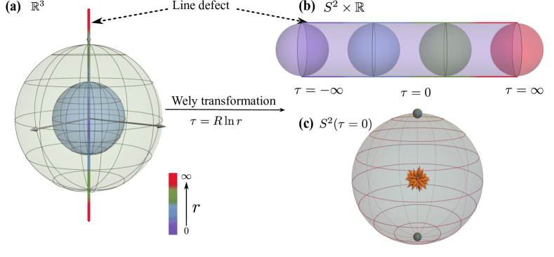
Figure 1: Schematic plot of the defect in 3D. Through a Weyl transformation, (a) Euclidean flat space-time $\mathbb{R}^{3}$ is mapped to (b) the cylinder manifold $S^{2}\times\mathbb{R}$. The line defect before and after the Weyl transformation are shown by the colored line. (c) The $0+1$-D impurities (cyan point) located at the north and south pole on two-dimensional sphere $S^{2}$ in the radial quantization, where the flux at the center represents the magnetic monopole defined in the fuzzy sphere model.

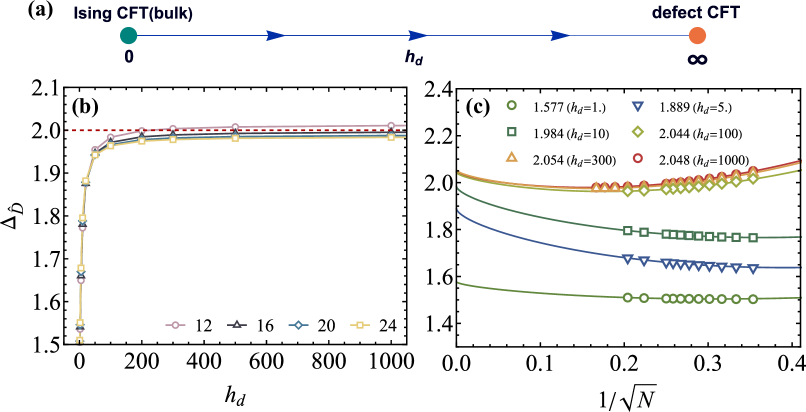
Figure 2: Defect induced attractive fixed point. (a) Schematic plot of the RG diagram. (b) The scaling dimension of displacement operator $\Delta_{\hat{D}}$ as a function of defect strength $h_{d}$. (c) Finite-size extrapolation of $\Delta_{\hat{D}}$ for various $h_{d}$ SM . A sufficient large $h_{d}$ gives almost identical $\Delta_{\hat{D}}\approx 2$, supporting an attractive RG fixed point at $h_{d}=\infty$.

Similar to the bulk CFT, we consider the radial quantization of a dCFT. Specifically, we first foliate the Euclidean space $\mathbb{R}^{3}$ using spheres $S^{2}$ with their origins situated on the defect, as illustrated in Fig. 1(a). Next, we can perform a Weyl transformation to map $\mathbb{R}^{3}$ to a cylinder $S^{2}\times\mathbb{R}$, and the $p$-dimensional defect transforms into a defect intersecting the cylinder. For instance, as shown in Fig. 1, the Weyl transformation maps a line defect ($p=1$) in $\mathbb{R}^{3}$ to $0+1$D point impurities located at the north and south poles of the sphere $S^{2}$, forming two continuous line cuts along the time direction from $\tau=-\infty$ to $\tau=\infty$. Similarly, a plane defect ($p=2$) in $\mathbb{R}^{3}$ will be mapped to a $1+1$D defect with its spatial component located on the equator of the sphere $S^{2}$.

Akin to the state-operator correspondence in bulk CFT Cardy (1984b, 1985), we have a one-to-one correspondence between the defect operators and the eigenstates of the dCFT quantum Hamiltonian on $S^{2}\times\mathbb{R}$, where energy gaps of these states are proportional to the scaling dimensions $\hat{\Delta}_{n}$ of the defect operators:

$$E_{n}-E_{0}=\frac{v}{R}\hat{\Delta}_{n}.$$ (3)

Here, $E_{0}$ denotes the ground state energy of the defect Hamiltonian, $R$ represents the sphere radius, and $v$ is a model-dependent non-universal velocity that corresponds to the arbitrary normalization of the Hamiltonian. Notably, this velocity $v$ is identical to the velocity of the bulk CFT Hamiltonian (further discussions see Supple. Mat. Sec. B SM ).

The state-operator correspondence offers distinct advantages for studying CFTs. Firstly, it provides direct access to information regarding whether the conformal symmetry emerges in the IR. Secondly, it enables an efficient extraction of various conformal data, such as scaling dimensions and OPE coefficients of primaries. The key step involves studying a quantum Hamiltonian on the sphere geometry. However, for 3D CFTs, this was challenging as no regular lattice could fit $S^{2}$. Recently, this fundamental obstacle was overcome through a scheme called “fuzzy sphere regularization” Zhu et al. (2023), and its superior capabilities have been convincingly demonstrated Zhu et al. (2023); Hu et al. (2023); Han et al. (2023); Zhou et al. (2023). Below we discuss how to adapt the fuzzy sphere regularization scheme to solve dCFTs. We will focus on the case of magnetic line defect of the 3D Ising CFT, but the generalizations to other cases should be straightforward.

Magnetic line defect on the fuzzy sphere.—The fuzzy sphere regularization Zhu et al. (2023) considers a quantum mechanical model describing fermions moving on a sphere with a $4\pi s$ magnetic monopole at the center. The model is generically described by a Hamiltonian $H=H_{\textrm{kin}}+H_{\textrm{int}}$, where $H_{\textrm{kin}}$ represents the kinetic energy of fermions, and its eigenstates form quantized Landau levels described by the monopole Harmonics $Y^{(s)}_{n+s,m}(\theta,\varphi)$ Wu and Yang (1976). Here, $n=0,1,\cdots$ denotes the Landau level index, and $(\theta,\varphi)$ are the spherical coordinates. We consider the limit where $H_{\textrm{kin}}$ is much larger than the interaction $H_{\textrm{int}}$, allowing us to project the system onto the lowest Landau level (i.e. $n=0$), resulting in a fuzzy sphere Madore (1992).

The 3D Ising transition on the fuzzy sphere can be realized by two-flavor fermions $\bm{\psi}^{\dagger}=(\psi_{\uparrow}^{\dagger},\psi_{\downarrow}^{\dagger})$ with interactions that mimic a 2+1D transverse Ising model on the sphere,

$$H_{0}= \int R^{4}d\Omega_{a}d\Omega_{b}\,U(\Omega_{ab})(n^{0}(\Omega_{a})n^{0}(\Omega_{b})-n^{z}(\Omega_{a})n^{z}(\Omega_{b}))$$

$$-h\int R^{2}d\Omega\,n^{x}(\Omega).$$ (4)

Here we are using the spherical coordinate $\Omega=(\theta,\phi)$ and $R$ is the sphere radius. The density operators are defined as $n^{\alpha}(\Omega)=\bm{\psi}^{\dagger}(\Omega)\sigma^{a}\bm{\psi}(\Omega)$, where $\sigma^{x,y,z}$ are the Pauli matrices and $\sigma^{0}$ is the identity matrix. $U(\Omega_{ab})$ encodes the Ising density-density interaction as $U(\Omega_{ab})=\frac{g_{0}}{R^{2}}\delta(\Omega_{ab})+\frac{g_{1}}{R^{4}}\nabla^{2}\delta(\Omega_{ab})$. One can tune the transverse field $h$ to realize a phase transition which falls into the 2+1D Ising universality class Zhu et al. (2023). In the following, we set $U(\Omega_{ab})$ and $h$ the same as the bulk Ising CFT that has been identified in Zhu et al. (2023).

To study the magnetic line defect of 3D Ising CFT, we add $0+1$D point-like magnetic impurities located at sphere’s north and south pole, modeled by a Hamiltonian term,

$$H_{d}=2\pi h_{d}(n^{z}(\theta=0,\varphi=0))+n^{z}(\theta=\pi,\varphi=0)),$$ (5)

where $h_{d}$ controls the strength of the magnetic impurities. This type of defect can be artificially realized in experiments Law (2001); Fisher and de Gennes . Crucially, the defect term $H_{d}$ breaks the Ising $\mathbb{Z}_{2}$ symmetry, causing the $\sigma$ field (of the 3D Ising CFT) to be turned on at the defect. This $\sigma$ deformation is relevant on the line defect ($\Delta_{\sigma}\approx 0.518<1$ Poland et al. (2019)), driving the system to flow to a nontrivial fixed point, conjectured to be a conformal defect. This fixed point is expected to be an attractive fixed point Allais and Sachdev (2014); Hanke (2000); Cuomo et al. (2022a), implying that regardless of the strength of $h_{d}$, the defect will flow to the same conformal defect fixed point (see Fig. 2(a)). Next we will provide compelling numerical evidence to support this conjecture.

The model $H_{0}+H_{d}$ for the magnetic line defect of 3D Ising CFT is a continuous model with fully local interaction in the spatial space. In practice, we consider the second quantization form of this model by the projecting $H_{0}+H_{d}$ to the lowest Landau level (fuzzy sphere), using $\psi_{a}(\Omega)=\frac{1}{\sqrt{N}}\sum_{m=-s}^{s}c_{m,a}Y^{(s)}_{s,m}(\Omega)$ (we are using a slightly different convention compared to Ref. Zhu et al. (2023)). Here $N=2s+1$ playing the role of system size $N\sim R^{2}$, and we simply replace $R^{2}$ with $N$ during the projection. This lowest Landau level projection leads to a second quantized Hamiltonian defined by fermionic operators $c_{m,a}$, and similar models have been extensively studied in the context of the quantum Hall effect Haldane (1983). Numerically, this model can be simulated using various techniques such as exact diagonalization and density matrix renormalization group (DMRG) White (1992); Feiguin et al. (2008). We perform DMRG calculations with bond dimensions up to $D=5000$, and for the largest system size $N=36$, the maximum truncation errors for the ground state and the tenth excited state are $1.37\times 10^{-9}$ and $1.96\times 10^{-8}$, respectively. We explicitly impose two $U(1)$ symmetries, i.e., fermion number and $SO(2)$ angular momentum.

Emergent conformal symmetry and operator spectrum.— The energy spectrum of the defect Hamiltonian ($H_{0}+H_{d}$) is expected to be proportional to the defect operators’ scaling dimensions, up to a non-universal velocity in Eq. (3). Here we determine the velocity using the bulk CFT Hamiltonian ($H_{0}$) by setting the $\sigma$ state to have $\Delta_{\sigma}=0.518149$ Poland et al. (2019). The defect term $H_{d}$ breaks the sphere rotation $SO(3)$ down to $SO(2)$, so each eigenstate has a well defined $SO(2)$ quantum number $L_{z}$. Akin to the stress tensor of the bulk CFT, there exists a special primary operator in dCFT due to the broken of translation symmetry, dubbed the displacement operator $\hat{D}$ Billó et al. (2013); Billò et al. (2016); McAvity and Osborn (1995), which has $L_{z}=\pm 1$ and a protected scaling dimension $\Delta_{\hat{D}}=2$. Fig. 2(b-c) depicts $\Delta_{\hat{D}}$ via the state-operator correspondence (Eq. (3)) for various defect strength $h_{d}$ and system sizes. It clearly shows that the obtained $\Delta_{\hat{D}}$ are very close to $2$, for different defect strengths $h_{d}$, which indicates an attractive conformal fixed point at $h_{d}=\infty$ (see Supple. Mat. Sec. C SM ). In what follows, we present the representative results for $h_{d}=300$ and we ensure the conclusions are insensitive to the choice of $h_{d}$.

Table 1: Scaling dimensions of primary operators in the magnetic line defect of 3D Ising CFT, determined through the state-operator correspondence on the fuzzy sphere. Please see a detailed analysis of errors and finite-size extrapolation in Supple. Mat. Sec. B-C SM .

$L_{z}=0$			$L_{z}=1$
$\hat{\phi}$	$\hat{\phi}^{\prime}$	$\hat{\phi}^{\prime\prime}$	$\hat{D}$	$\hat{\phi}_{1}$	$\hat{\phi}_{1}^{\prime}$
1.63(6)	3.12(10)	4.06(18)	2.05(7)	3.58(7)	4.64(14)

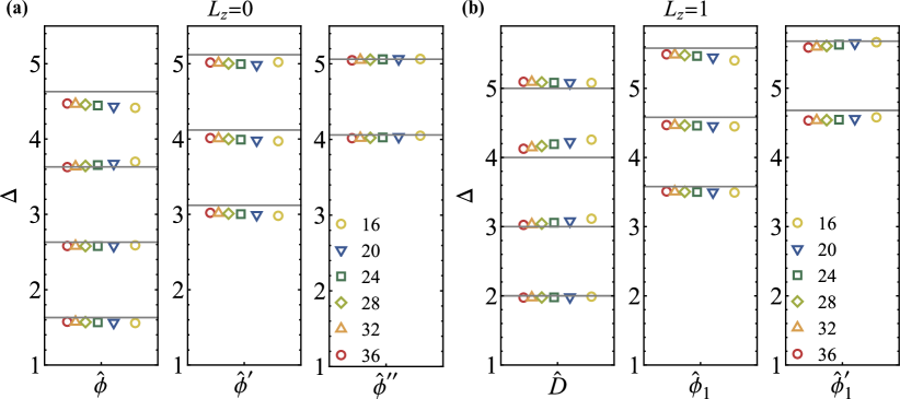
Figure 3: Conformal tower of defect primaries. Defect primary fields and their descendants with global symmetry (a) $L_{z}=0$ and (b) $L_{z}=1$. The grey horizon lines stand for the theoretical expectation for descendants. Different colored symbols represent the results based on various system sizes. By increasing system size $N$ all of scaling dimensions approach the theoretical values consistently, supporting an emergent conformal symmetry in the thermodynamic limit.

We further establish the emergent conformal symmetry by confirming that the excitation spectra form representations of $SO(2,1)$. The generators of $SO(2,1)$ are the dilation $D$, translation $P$, and special conformal transformation $K$. It is important to note that $P$ and $K$ do not have any Lorentz index due to the triviality of the Lorentz symmetry, i.e., $SO(1)$. For each primary operator, we have descendants generated by the translation, $P^{n}\hat{O}$, whose scaling dimension is $\Delta_{P^{n}\hat{O}}=\Delta_{\hat{O}}+n$, and its $SO(2)$ quantum number $L_{z}$ remains unchanged. Fig. 3 displays our numerical data of the low-lying energy spectrum, clearly exhibiting the emergent conformal symmetry, i.e., approximate integer spacing between each primary and its descendants. These observations firmly establish that the magnetic line defect of the 3D Ising CFT flows to a conformal defect with a conformal symmetry of $SO(2,1)$.

From our numerical data, we are able to identify five low-lying defect primary operators in addition to $\hat{D}$, as listed in Tab. 1. Notably, all these operators are found to be irrelevant (i.e., $\Delta>1$), which is consistent with the observation of an attractive defect fixed point. Our lowest-lying operator $\hat{\phi}$ has $L_{z}=0$ and $\Delta_{\hat{\phi}}\approx 1.63(6)$. This value is in good agreement with Monte Carlo simulations, e.g. $1.60(5)$ Parisen Toldin et al. (2017), $1.52(6)$ Parisen Toldin et al. (2017), and $1.40(3)$ Allais (2014), as well as with the perturbative $\varepsilon$-expansion computation of $\sim 1.55(14)$ Ref. Cuomo et al. (2022a). The second low-lying operator in the $L_{z}=0$ sector has $\Delta_{\hat{\phi^{\prime}}}=3.12(10)$, which significantly deviates from the $\varepsilon$-expansion value of $\Delta\approx 4.33+O(\varepsilon^{2})$ (it was called $\hat{s}_{+}$ in  Cuomo et al. (2022a)). This suggests a large sub-leading correction in the $\varepsilon$-expansion. All other primary operators identified in our study are new and have not been computed by any other methods. It is essential to mention that the scaling dimensions in Tab. 1 are obtained by the finite-size extrapolating (see details in Supple. Mat. Sec. B SM ), and the data at finite $N$ is already very close to the extrapolated value (The finite-size extrapolation improve the results by around $2\%$). One can also improve the accuracy by making use of conformal perturbation Lao and Rychkov (2023).

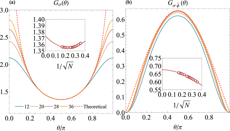
Figure 4: Correlators involving defect. The angle dependence of (a) correlator $G_{\sigma}(\theta)$ and (b) $G_{\sigma\hat{\phi}}(\theta)$, for system sizes ranging from $N=12$ to $36$. The dashed lines correspond to theoretical correlator in Eq. (6) with $b_{\sigma\hat{O}_{2}}$ and $\Delta_{\hat{O}_{2}}$ from the $N=36$ curves. The insets are finite-size scaling analysis by setting $\theta=\pi/2$, respectively giving one-point OPE coefficient $a_{\sigma}\approx 1.37(1)$ and bulk-defect OPE coefficient $b_{\sigma\hat{\phi}}\approx 0.68(1)$.

Correlators and OPE coefficients.— Using Weyl transformation, we can map the bulk-defect correlators in Eq. (1), Eq. (2) in $\mathbb{R}^{3}$ to the correlators on cylinder $S^{2}\times\mathbb{R}$ (see Supple. Mat. Sec. A SM ),

$$G_{O_{1}\hat{O}_{2}}\equiv\frac{\langle\hat{\mathbf{1}}|O_{1}(\tau=0,\theta)|\hat{O}_{2}\rangle}{\langle\mathbf{1}|O_{1}(\tau=0,\theta)|O_{1}\rangle}=\frac{b_{O_{1}\hat{O}_{2}}}{(\sin\theta)^{\Delta_{1}-\hat{\Delta}_{2}}}.$$ (6)

The bulk operator $O_{1}$ is positioned at a point that has an angle $\theta$ with respect to the north pole. In the denominator, we use the states of the bulk CFT, while in the numerator, we use the states of the dCFT. The one-point bulk correlator corresponds to taking $|\hat{O}_{2}\rangle$ to be the ground state of the defect, i.e., $|\hat{\mathbf{1}}\rangle$.

In the fuzzy sphere model, we can use the spin operators $n^{z}$ and $n^{x}$ to approximate the bulk CFT primary operators $\sigma$ and $\epsilon$ Hu et al. (2023); Han et al. (2023). For example, the correlator between the bulk primary $\sigma$ and a defect primary operator $\hat{O}_{2}$ is computed by,

$$G_{\sigma\hat{O}_{2}}\equiv\frac{\langle\hat{\mathbf{1}}|n^{z}(\tau=0,\theta)|\hat{O}_{2}\rangle}{\langle\mathbf{1}|n^{z}(\tau=0,\theta)|\sigma\rangle}=\frac{b_{\sigma\hat{O}_{2}}}{(\sin\theta)^{\Delta_{\sigma}-\hat{\Delta}_{2}}}+O(N^{-1/2}).$$ (7)

Here, $\Delta_{\sigma}\approx 0.518149$, and the first-order correction $O(N^{-1/2})$ comes from the descendant operator $\partial_{\mu}\sigma$ contained in $n^{z}$. Fig. 4 illustrates the one-point bulk correlator $G_{\sigma}(\theta)$ and bulk-defect correlator $G_{\sigma\hat{\phi}}(\theta)$ for different system sizes $N=12-36$. Both correlators agree perfectly with the CFT prediction Eq.(6), except for the small $\theta$ regime. It is worth noting that the one-point correlator $G_{\sigma}(\theta)$ is divergent at $\theta=0,\pi$ and reaches a minimum at $\theta=\pi/2$. In contrast, the bulk-defect correlator $G_{\sigma\hat{\phi}}(\theta)$ has an opposite behavior (because $\Delta_{\sigma}-\Delta_{\hat{\phi}}<0$); it vanishes at $\theta=0,\pi$ and reaches a maximum at $\theta=\pi/2$. These behaviors are nicely reproduced in our data, which is highly nontrivial because computationally the only difference for the two correlators is the choice of $|\hat{O}_{2}\rangle$ in Eq. (7).

Table 2: Bulk-to-defect OPE coefficients magnetic line defect of 3D Ising CFT. $C_{\hat{D}}$ is computed by Eq. (8) using $\sigma$ and $\epsilon$.

$a_{\sigma}$	$b_{\sigma\hat{\phi}}$	$a_{\epsilon}$	$b_{\epsilon\hat{\phi}}$	$C_{\hat{D}}$ by $\sigma$	$C_{\hat{D}}$ by $\epsilon$
1.37(1)	0.68(1)	1.31(19)	1.63(4)	0.53(3)	0.59(18)

We can further extract the bulk-defect OPE coefficients from $G_{O_{1}\hat{O}_{2}}(\theta=\pi/2)=b_{O_{1}\hat{O}_{2}}$, and the results are summarized in Tab. 2. None of these OPE coefficients was computed non-perturbatively before. There are perturbative computations for $a_{\sigma}$ and $a_{\epsilon}$ Cuomo et al. (2022a) from $\varepsilon$ expansion, giving $a_{\sigma}^{2}\approx 3.476+O(\varepsilon^{2})$ (i.e. $a_{\sigma}\approx 1.86$) and $a_{\epsilon}\approx 1.83+O(\varepsilon^{2})$. Our estimates are $a_{\sigma}=1.37(1)$ and $a_{\epsilon}=1.31(19)$, it will be interesting to compute higher order corrections in the $\varepsilon$-expansion. Moreover, using the Ward identity of any bulk operator ($O$) Billò et al. (2016), we can extract Zamolodchikov norm

$$\sqrt{C_{\hat{D}}}=\frac{2}{\pi}\frac{\Delta_{O}G_{O}(\theta=\pi/2)}{G_{O\hat{D}}(\theta=\pi/2)}.$$ (8)

The estimates using $\sigma$ and $\epsilon$ gives $C_{\hat{D}}=0.53(3)$ and $C_{\hat{D}}=0.59(18)$, respectively.

Summary and discussion.— We have outlined a systematic procedure to study defect conformal field theory (dCFT) using the recently-proposed fuzzy sphere regularization scheme. As a concrete application, we investigated the magnetic line defect of 3D Ising CFT and provided clear evidence that it flows to a conformal defect. Crucially, we accurately computed a number of new conformal data of this dCFT, including defect primaries’ scaling dimensions and bulk-defect OPE coefficients. The current setup can be readily applied to the study of various types of defects in distinct 3D CFTs, potentially resolving numerous open questions and offering new insights into defects in CFTs.

Acknowledgments.— We thank Davide Gaiotto for stimulating discussions that initiated this project. LDH and WZ were supported by National Natural Science Foundation of China (No. 92165102, 11974288) and National key R$\&$D program (No. 2022YFA1402204). Research at Perimeter Institute is supported in part by the Government of Canada through the Department of Innovation, Science and Industry Canada and by the Province of Ontario through the Ministry of Colleges and Universities. YCH thanks the hospitality of Bootstrap 2023 at ICTP South American Institute for Fundamental Research, where part of this project was done.

Supplementary Material for “Solving Conformal Defects in 3D Conformal Field Theory using Fuzzy Sphere Regularization”

In this supplementary material, we will show more details to support the discussion in the main text. In Sec. A, we discuss the defect CFT correlators on the cylinder $S^{2}\times\mathbb{R}$. In Sec. B, we present an error analysis of the scaling dimensions of defect primaries. In Sec. C, we provide in-depth analysis of the attractive fixed point induced by the line defect. In Sec. D., we show the operator product expansion (OPE) related to the primary $\epsilon$. In Sec. E. we present the computation of Zamolodchikov norm regarding to the displacement operator.

Appendix A A. Bulk to defect correlators

In this section, we present the correlators of primary operators in the dCFT on the cylinder $S^{2}\times\mathbb{R}$ by using the state-operator correspondence. As discussed in the main text, by introducing of a flat $p$-dimensional defect breaks the global conformal symmetry $SO(4,1)$ into $SO(p+1,1)\times SO(3-p)$. Making use of state-operator correspondence, the bulk-defect (scalar-scalar) correlator $\langle O_{1}(x)\hat{O}_{2}(0)\rangle=\frac{b_{O_{1}\hat{O}_{2}}}{|x_{\perp}|^{\Delta_{1}-\hat{\Delta}_{2}}|x|^{2\hat{\Delta}_{2}}}$ can be mapped to

$$\langle\hat{\mathbf{1}}|O_{1}(x)|\hat{O}_{2}\rangle=\frac{b_{O_{1}\hat{O}_{2}}}{|x_{\perp}|^{\Delta_{1}-\hat{\Delta}_{2}}|x|^{2\hat{\Delta}_{2}}}$$ (S1)

where $|\hat{\mathbf{1}}\rangle$ is the vacuum state of the dCFT.

Next, we apply the Weyl transformation $\tau=R\ln r$ to map the coordinates $(r,\theta,\varphi)$ in $\mathbb{R}^{3}$ to $(\tau,\theta,\varphi)$ in $S^{2}\times\mathbb{R}$, where $R$ is the radius of $S^{2}$. Under the Weyl transformation, the operator transforms as:

$$\phi(r,\theta,\varphi)\rightarrow\phi(\tau,\theta,\varphi)=\Lambda(r,\theta,\varphi)^{\Delta/2}\phi(r,\theta,\varphi),$$ (S2)

where $\Lambda=R^{-2}e^{\frac{2\tau}{R}}$ represents the scale factor of this transformation. Substituting this into the correlator and setting $\tau=0$, we get:

$$\langle\hat{\mathbf{1}}|O_{1}(\tau=0,\theta,\varphi)|\hat{O}_{2}\rangle=\langle\hat{\mathbf{1}}|\Lambda(r,\theta,\varphi)^{\Delta_{1}/2}O_{1}(r,\theta,\varphi)|\hat{O}_{2}\rangle\big{|}_{r=1}=R^{-\Delta_{1}}\frac{b_{O_{1}\hat{O}_{2}}}{|\sin\theta|^{\Delta_{1}-\hat{\Delta}_{2}}}$$ (S3)

On the hand, we have $\langle{\mathbf{1}}|O_{1}(\tau=0,\theta,\varphi)|O_{1}\rangle=R^{-\Delta_{1}}$ for the bulk CFT, so we finally have,

$$G_{O_{1}\hat{O}_{2}}\equiv\frac{\langle\hat{\mathbf{1}}|O_{1}(\tau=0,\theta,\varphi)|\hat{O}_{2}\rangle}{\langle\mathbf{1}|O_{1}(\tau=0,\theta,\varphi)|O_{1}\rangle}=\frac{b_{O_{1}\hat{O}_{2}}}{(\sin\theta)^{\Delta_{1}-\hat{\Delta}_{2}}}$$ (S4)

Lastly, it is noting that, for the flat line defect ($d=1$) breaking the symmetry into $SO(2,1)\times SO(2)$, the defect operator can have a non-trivial $SO(2)$ quantum number $L_{z}=m$. For such a defect operator, we have,

$$G_{O_{1}\hat{O}_{2}}\equiv\frac{e^{-im\varphi}\langle\hat{\mathbf{1}}|O_{1}(\tau=0,\theta,\varphi)|\hat{O}_{2},L_{z}=m\rangle}{\langle\mathbf{1}|O_{1}(\tau=0,\theta,\varphi)|O_{1}\rangle}=\frac{b_{O_{1}\hat{O}_{2}}}{(\sin\theta)^{\Delta_{1}-\hat{\Delta}_{2}}},$$ (S5)

where the bulk operator $O_{1}$ is still a Lorentz scalar.

Appendix B B. Error analysis

B.1 1. Scaling dimension

In this section, we provide a detailed analysis of the scaling dimensions of primaries and offer a way to estimate the error of the obtained numerical data. In general, in this work we use two different methods to obtain the scaling dimensions of the defect primaries, which gives consistent results.

These three methods are described as below.

1. Since the scaling dimension of displacement operator is expected to be $\Delta_{\hat{D}}=2$, we can set the dimension of displacement operator to $\Delta_{\hat{D}}=2$ and rescale the energy spectrum. The obtained results of low-lying defect primaries are shown in the first line of Table S1.

2. We assume that the presence of defect does not affect the velocity of spectra, so we let $v_{\text{def}}=v_{\text{bulk}}$. So we determine the scaling dimensions $\Delta_{\hat{O}}$ through

   $$E_{\hat{O}}-E_{\hat{\mathbf{1}}}=\frac{\Delta_{\hat{O}}}{R}v_{\text{bulk}},$$

   where $v_{\text{bulk}}$ is determined by the bulk Ising CFT Zhu et al. (2023). That is, after extracting the velocity $v_{\text{bulk}}$, the scaling dimensions of the dCFT is

   $$\Delta_{\hat{O}}=\frac{E_{\hat{O}}-E_{\hat{\mathbf{1}}}}{v_{\text{bulk}}}R=\frac{E_{\hat{O}}-E_{\hat{\mathbf{1}}}}{E_{\sigma}-E_{0}}\Delta_{\sigma},$$

   where $\Delta_{\sigma}=0.518149$ is for bulk primary $\sigma$ field. The results obtained in this way are displayed in the second line of Table S1. The consistency of methods 1 and 2 is a strong evidence of $v_{\text{def}}=v_{\text{bulk}}$. Throughout this article, we employ this method to compute the scaling dimensions.

The summary of the scaling dimensions obtained by above two methods are shown in Tab. S1.

Furthermore, to estimate the scaling dimensions in the thermodynamic limit, we apply a finite-size extrapolation analysis based on the method 2. Generally, we fit the scaling dimensions of primaries (obtained on finite-size $N$) using the following form (see section C):

$$\Delta_{\hat{O}}^{\text{Method 2}}(N)\approx\Delta_{\hat{O}}+\frac{b}{R^{\Delta_{\hat{\phi}}-1}}+\frac{c}{R^{\Delta_{\hat{\phi}^{\prime}}-1}}+\text{higher order corrections}$$ (S6)

where $b,c$ are non-universal parameters, $R\sim\sqrt{N}$. The finite-size scaling for several typical primaries are shown in Fig. S2. The scaling dimension in the thermodynamic limit $\Delta_{\hat{O}}$ can be extracted in this way.

At last, the relative error is estimated through the following comparison. The numerical error of the fitting process in Eq. S6 is $\delta\overline{\Delta}_{\hat{O}}$, which is determined by comparing the different fitting processes using various finite system sizes (five large system sizes are always included). We also compare different methods to determine the relative errors, e.g. difference between $\Delta_{\hat{O}}$ and $\Delta_{\hat{O}}^{\text{Method 1}}(N=36),\Delta_{\hat{O}}^{\text{Method 2}}(N=36)$ as the relative error. Finally, we use the maximum value of these estimates as the relative error:

$$\delta\Delta_{\hat{O}}=Max\{\delta\overline{\Delta}_{\hat{O}},|\Delta_{\hat{O}}-\Delta_{\hat{O}}^{\text{Method 1}}(N=36)|,|\Delta_{\hat{O}}-\Delta_{\hat{O}}^{\text{Method 2}}(N=36)|\}.$$ (S7)

We think this error represents the maximal relative error of the obtained scaling dimensionsin our numerical calculations.

Finally, the numerical estimation based on the finite-size extrapolation and corresponding error bars are presented in the Table I in the main text.

Table S1: The scaling dimensions of primaries in sector $L_{z}=0,1$. The first three lines correspond to method 1-3 in size $N=36$

	$L_{z}=0$			$L_{z}=1$
	$\hat{\phi}$	$\hat{\phi}^{\prime}$	$\hat{\phi}^{\prime\prime}$	$\hat{D}$	$\hat{\phi}_{1}$	$\hat{\phi}_{1}^{\prime}$
$\Delta_{\hat{O}}^{\text{Method 1}}(N=36)$	1.59	3.05	4.06	2	3.55	4.52
$\Delta_{\hat{O}}^{\text{Method 2}}(N=36)$	1.57	3.02	4.02	1.98	3.51	4.53

B.2 2. OPE coefficients

In this subsection, we delve into the finite size correction and error estimation of the OPE coefficients. Generally, the finite size correction arises from the descendants and higher primary operators. For instance, considering $\sigma$, the higher contributions involve $\partial_{\mu}\sigma$, $(\Box\sigma,\partial_{\mu}\partial_{\nu}\sigma)$, $(\partial_{\mu}\Box\sigma,\partial_{\mu}\partial_{\nu}\partial_{\rho}\sigma)$, $\sigma^{\prime}$, and so on. The corresponding bulk-defect OPE is given by:

$$G_{\sigma\hat{O}}(\theta)=\frac{\langle\mathbf{\hat{1}}|n^{z}|\hat{O}\rangle}{\langle\sigma|n^{z}|\mathbf{1}\rangle}\approx\frac{b_{\sigma\hat{O}}}{(\sin\theta)^{\Delta_{\sigma}-\Delta_{\hat{O}}}}\left(1+\frac{1}{R}+\frac{1}{R^{2}}+\frac{1}{R^{3}}+O(1/R^{4.180-0.518})\right).$$ (S8)

Similarly, for the higher correction from $\partial_{\mu}\epsilon$, $T_{\mu\nu}$, $(\Box\epsilon,\partial_{\mu}\partial_{\nu}\epsilon)$, $\epsilon^{\prime}$, and so on, we have:

$$G_{\epsilon\hat{O}}(\theta)=\frac{\langle\mathbf{\hat{1}}|n^{x}|\hat{O}\rangle-\delta_{\hat{O}\mathbf{\hat{1}}}\langle\mathbf{\hat{1}}|n^{x}|\mathbf{\hat{1}}\rangle}{\langle\epsilon|n^{x}|\mathbf{1}\rangle}\approx\frac{b_{\epsilon\hat{O}}}{(\sin\theta)^{\Delta_{\epsilon}-\Delta_{\hat{O}}}}\left(1+\frac{1}{R}+\frac{1}{R^{3-1.413}}+\frac{1}{R^{2}}+O(1/R^{3.830-1.413})\right).$$ (S9)

Regarding the error bar estimation, we perform the finite size extrapolation using the first two powers to obtain the OPE coefficients $b_{O\hat{O}_{n}}$. We compare various fitting processes by considering different finite system sizes used in the finite-size extrapolations (the five largest system sizes are always included). By comparing the extrapolated OPE coefficients obtained by different fitting processes, we calculate the standard value and corresponding error bar.

Appendix C C. Attractive fixed point

In this section, we aim to demonstrate numerically that the Ising CFT with a line defect possesses an attractive fixed point under the flow of $h_{d}$.

Firstly, we ensure that, under the magnetic line defect the low-energy excitation spectrum is gapless. This can be examined through the scaling analysis, as illustrated in Fig. S1.

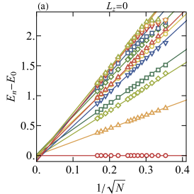
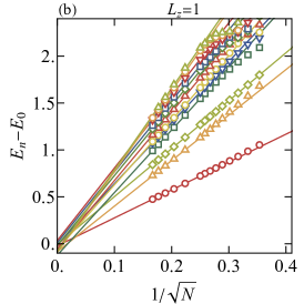
Figure S1: Energy gap scaling. The finite-size scaling of energy gap $E_{n}-E_{0}$ for the first $10$ states in sector (a)$L_{z}=0$ and (b)$L_{z}=1$. System sizes from $N=8$ to $N=15$ (ED) and $N=16$ to $N=36$ (DMRG with $D=5000$). Here we set $h_{d}=300$.

Second, we examine how the scaling dimensions of primaries converge to the same values for various $h_{d}$. Finite size corrections arise from irrelevant operators with scaling dimensions $\Delta_{\hat{O}}>1$. Among these operators, the lowest two primaries are $\hat{\phi}$ and $\hat{\phi}^{\prime}$. Consequently, the finite size correction to the scaling dimension can be approximated as follows:

$$\Delta_{\hat{O}}(N)\approx\Delta_{\hat{O}}+\frac{b}{R^{\Delta_{\hat{\phi}}-1}}+\frac{c}{R^{\Delta_{\hat{\phi}^{\prime}}-1}}+\text{higher order corrections}.$$ (S10)

By employing this relation and setting $\hat{O}=\hat{\phi},\hat{\phi}^{\prime}$, we obtain two consistency equations which give the scaling dimensions $\Delta_{\hat{\phi}},\Delta_{\hat{\phi}^{\prime}}$. For example, we obtain for $h_{d}=300$:

$$\Delta_{\hat{\phi}}\approx 1.63\quad\text{and}\quad\Delta_{\hat{\phi}^{\prime}}\approx 3.12.$$ (S11)

Subsequently, by applying this approach to various values of $h_{d}$ ranging from $1$ to $1000$, we observe that the scaling dimensions of $\hat{\phi}$ and $\hat{\phi}^{\prime}$ are insensitive to $h_{d}$. Finally, we examine the displacement operator $\hat{D}$ in the $L_{z}=1$ sector. The exact value is $\Delta_{\hat{D}}=2$, and the numerical results closely match $2$ with very high precision. These findings, the scaling dimensions insensitive to the defect strength $h_{d}$, provide compelling evidence for the existence of an attractive fixed point in the presence of a line defect. All the results are presented in Figure (S2).

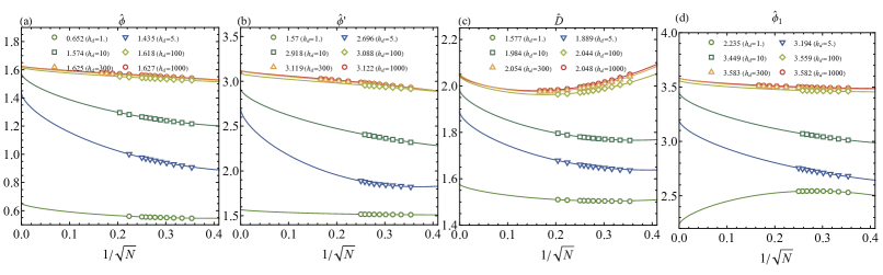
Figure S2: Finite-size correction of scaling dimensions for the lower primaries: (a) $\hat{\phi}$, (b) $\hat{\phi}^{\prime}$, (c) $\hat{D}$, and (d) $\hat{\phi}_{1}$, are determined using Eq. (S10). For different values of $h_{d}$, each primary converges to the same value, indicating the nature of an attractive fixed point.

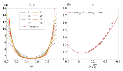
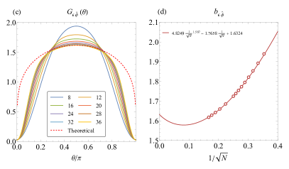
Figure S3: Correlators related to $\epsilon$ (a-b) The one-point correlator $a_{\epsilon}$ and its finite-size extrapolation. The result is $a_{\epsilon}\approx 1.31$. (c-d) The bulk-defect correlator $G_{\epsilon\hat{\phi}}(\theta)$ with a resulting coefficient of $b_{\epsilon\hat{\phi}}\approx 1.63$. The dashed lines correspond to the theoretical correlator in Eq. (S12) with $b_{\epsilon\hat{O}}$ and $\Delta_{\hat{O}}$ from the $N=36$ curves. The system size ranges from $N=8$ to $N=36$($D=5000$).

Appendix D D. Numerical results of correlators of $\epsilon$

In the main text, we have shown the correlators and OPE coefficients related to $\sigma$ (Fig. 4 and related discussion). In this section, we present the correlators and OPE coefficients related to the bulk operator $\epsilon$. Following the method described in the main text and in Ref. Hu et al. (2023), we approximate it using the operator $n^{x}(\Omega)$. The one-point and bulk-defect OPE are given by:

$$\begin{split}G_{\epsilon}(\theta)&=\frac{\langle\mathbf{\hat{1}}|n^{x}|\mathbf{\hat{1}}\rangle-\langle\mathbf{1}|n^{x}|\mathbf{1}\rangle}{\langle\epsilon|n^{x}|\mathbf{1}\rangle}\approx\frac{a_{\epsilon}}{(\sin\theta)^{\Delta_{\epsilon}}}+O(1/R)\\ G_{\epsilon\hat{O}}(\theta)&=\frac{\langle\mathbf{\hat{1}}|n^{x}|\hat{O}\rangle}{\langle\epsilon|n^{x}|\mathbf{1}\rangle}\approx\frac{b_{\epsilon\hat{O}}}{(\sin\theta)^{\Delta_{\epsilon}-\Delta_{\hat{O}}}}+O(1/R)\end{split}$$ (S12)

Please note that the operator $n^{x}$ includes an identity component that should be subtracted. Since $\Delta_{\epsilon}\approx 1.413>0$, $G_{\epsilon}(\theta)$ should diverge at $\theta=0,\pi$. This behavior is also observed in Fig. S3(a). We calculated $G_{\epsilon}(\theta)$ and extracted the OPE coefficient using $a_{\epsilon}=G_{\epsilon}(\pi/2)$. In order to perform the finite-size extrapolation, we need to consider the finite-size correction given by:

$$G_{\epsilon}(\theta)\approx\frac{1}{(\sin\theta)^{\Delta_{\epsilon}-\Delta_{\hat{O}}}}\left(b_{\epsilon\hat{O}}+\frac{b_{\partial\epsilon\hat{O}}}{R}+\frac{b_{T_{\mu\nu}\hat{O}}}{R^{3-1.413}}+O(1/R^{2})\right)$$ (S13)

where the first pole $1/R$ comes from $\partial\epsilon$ and the second pole comes from $T_{\mu\nu}$. After the finite-size extrapolation, we find $a_{\epsilon}\approx 1.31$.

Next, we consider the bulk-defect OPE. Since the lowest primary in dCFT is $\Delta_{\hat{\phi}}\approx 1.64>\Delta_{\epsilon}$, the correlator $G_{\epsilon\hat{O}}(\theta)$ is zero at $\theta=0,\pi$. We present the result for $G_{\epsilon\hat{\phi}}$ in Fig. S3(c), and the finite-size correction follows the same analysis as described above, yielding $b_{\epsilon\hat{\phi}}\approx 1.63$.

Appendix E E. Ward identity regarding to the displacement operator

In dCFT, the displacement operator is related to the stress tensor in the bulk CFT, $\partial_{\mu}T_{\mu\nu}(x_{\perp},x_{\parallel})=\delta(x_{\perp})\hat{D}(x_{\parallel})$. The stress-tensor has a canonical normalization through the Ward-identity, so the normalization of $\hat{D}$ is also fixed. Therefore, the two-point correlator of displacement operator will not be normalized to $1$, instead, it is

$$\langle\hat{D}(x)\hat{D}(0)\rangle=C_{\hat{D}}\frac{1}{x^{4}},$$ (S14)

where the normalization factor $C_{\hat{D}}$ is the Zamolodchikov norm Billò et al. (2016) or central charge. For this canonically normalized displacement operator, its bulk-defect OPE coefficients are constrained by the Ward identity Billò et al. (2016):

$$\Delta_{O}a_{O}=\frac{\pi}{2}b_{O\hat{D}},$$ (S15)

where $O$ is a bulk scalar primary operator. In our fuzzy sphere computation, the state of displacement operator is naturally normalized to 1, i.e., $\langle\hat{D}|\hat{D}\rangle=1$, so we shall have,

$$|\hat{D}\rangle=\frac{1}{\sqrt{C_{\hat{D}}}}\hat{D}(\tau=-\infty)|\hat{\mathbf{1}}\rangle.$$ (S16)

Therefore, we can extract $C_{\hat{D}}$ using

$$\sqrt{C_{\hat{D}}}=\frac{2}{\pi}\frac{\Delta_{O}G_{O}(\theta=\pi/2)}{G_{O\hat{D}}(\theta=\pi/2)},$$ (S17)

where,

$$G_{O\hat{D}}\equiv\frac{e^{-i\varphi}\langle\hat{\mathbf{1}}|O(\tau=0,\theta,\varphi)|\hat{D}\rangle}{\langle\mathbf{1}|O(\tau=0,\theta,\varphi)|O\rangle},$$ (S18)

The results are depicted in Fig. S4(c). For comparison, we calculate the results by setting $O=\sigma$ and $O=\epsilon$, yielding $C_{\hat{D}}=0.53(3)$ for $O=\sigma$ and $C_{\hat{D}}=0.59(18)$ for $O=\epsilon$.

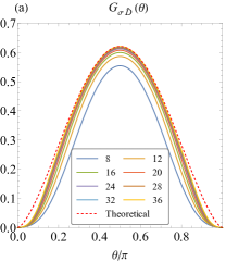
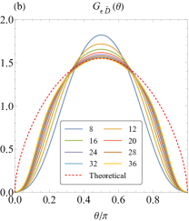
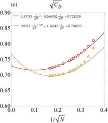
Figure S4: Correlators between the displacement operator and bulk operator: (a) $O=\sigma$ and (b) $O=\epsilon$. The dashed lines correspond to the theoretical correlator in Eq. S12 with $b_{\epsilon\hat{D}}$ and $\Delta_{\hat{D}}$ from the $N=36$ curves. (c) The extracted Zamolodchikov norm from Eq. S17. The red circles represent the results obtained when $O=\sigma$, while the yellow triangles correspond to the results when $O=\epsilon$.

References

- Wilson (1975) Kenneth G. Wilson, “The renormalization group: Critical phenomena and the kondo problem,” Rev. Mod. Phys. 47, 773–840 (1975).
- Nayak et al. (2008) Chetan Nayak, Steven H. Simon, Ady Stern, Michael Freedman, and Sankar Das Sarma, “Non-abelian anyons and topological quantum computation,” Rev. Mod. Phys. 80, 1083–1159 (2008).
- Hasan and Kane (2010) M. Z. Hasan and C. L. Kane, “Colloquium: Topological insulators,” Rev. Mod. Phys. 82, 3045–3067 (2010).
- Qi and Zhang (2011) Xiao-Liang Qi and Shou-Cheng Zhang, “Topological insulators and superconductors,” Rev. Mod. Phys. 83, 1057–1110 (2011).
- Wilson (1974) Kenneth G. Wilson, “Confinement of quarks,” Phys. Rev. D 10, 2445–2459 (1974).
- Hooft (1978) Gerard’t Hooft, “On the phase transition towards permanent quark confinement,” Nuclear Physics: B 138, 1–25 (1978).
- Maldacena (1999) Juan Maldacena, “The large-n limit of superconformal field theories and supergravity,” International Journal of Theoretical Physics 38, 1113–1133 (1999).
- Holzhey et al. (1994) Christoph Holzhey, Finn Larsen, and Frank Wilczek, “Geometric and renormalized entropy in conformal field theory,” Nuclear Physics B 424, 443 – 467 (1994).
- Calabrese and Cardy (2004) Pasquale Calabrese and John Cardy, “Entanglement entropy and quantum field theory,” Journal of Statistical Mechanics: Theory and Experiment 2004, P06002 (2004).
- Philippe Francesco (1997) David Sénéchal Philippe Francesco, Pierre Mathieu, Conformal Field Theory, Graduate Texts in Contemporary Physics (Springer New York, NY, 1997).
- Cardy (1996) J. Cardy, Scaling and Renormalization in Statistical Physics (Cambridge University Press, Cambridge, England, 1996).
- Cardy (1984a) John L. Cardy, “Conformal invariance and surface critical behavior,” Nuclear Physics B 240, 514–532 (1984a).
- Cardy (1989) John L. Cardy, “Boundary conditions, fusion rules and the verlinde formula,” Nuclear Physics B 324, 581–596 (1989).
- Cardy and Lewellen (1991) John L. Cardy and David C. Lewellen, “Bulk and boundary operators in conformal field theory,” Physics Letters B 259, 274–278 (1991).
- Diehl and Dietrich (1981) H. W. Diehl and S. Dietrich, “Field-theoretical approach to multicritical behavior near free surfaces,” Phys. Rev. B 24, 2878–2880 (1981).
- McAvity and Osborn (1993) D. M. McAvity and H. Osborn, “Energy-momentum tensor in conformal field theories near a boundary,” Nuclear Physics B 406, 655–680 (1993), arXiv:hep-th/9302068 [hep-th] .
- McAvity and Osborn (1995) D.M. McAvity and H. Osborn, “Conformal field theories near a boundary in general dimensions,” Nuclear Physics B 455, 522–576 (1995).
- Billó et al. (2013) M. Billó, M. Caselle, D. Gaiotto, F. Gliozzi, M. Meineri, and R. Pellegrini, “Line defects in the 3d Ising model,” Journal of High Energy Physics 2013, 55 (2013), arXiv:1304.4110 [hep-th] .
- Billò et al. (2016) Marco Billò, Vasco Gonçalves, Edoardo Lauria, and Marco Meineri, “Defects in conformal field theory,” Journal of High Energy Physics 2016, 91 (2016), arXiv:1601.02883 [hep-th] .
- Liendo et al. (2013) P. Liendo, L. Rastelli, and B.C. van Rees, “The bootstrap program for boundary CFTd.” Journal of High Energy Physics 2013, 113 (2013).
- Poland et al. (2019) David Poland, Slava Rychkov, and Alessandro Vichi, “The conformal bootstrap: Theory, numerical techniques, and applications,” Rev. Mod. Phys. 91, 015002 (2019).
- Gaiotto et al. (2014) D. Gaiotto, D. Mazac, and M.F. Paulos, “Bootstrapping the 3d Ising twist defect.” Journal of High Energy Physics 2014, 100 (2014).
- Gliozzi et al. (2015) Ferdinando Gliozzi, Pedro Liendo, Marco Meineri, and Antonio Rago, “Boundary and Interface CFTs from the Conformal Bootstrap,” Journal of High Energy Physics 2015, 36 (2015).
- Padayasi et al. (2022) Jaychandran Padayasi, Abijith Krishnan, Max Metlitski, Ilya Gruzberg, and Marco Meineri, “The extraordinary boundary transition in the 3d O(N) model via conformal bootstrap,” SciPost Physics 12, 190 (2022), arXiv:2111.03071 [cond-mat.stat-mech] .
- Gimenez-Grau et al. (2022) Aleix Gimenez-Grau, Edoardo Lauria, Pedro Liendo, and Philine van Vliet, “Bootstrapping line defects with O(2) global symmetry,” Journal of High Energy Physics 2022, 18 (2022), arXiv:2208.11715 [hep-th] .
- Affleck and Ludwig (1991) Ian Affleck and Andreas W. W. Ludwig, “Universal noninteger “ground-state degeneracy” in critical quantum systems,” Phys. Rev. Lett. 67, 161–164 (1991).
- Vojta et al. (2000) Matthias Vojta, Chiranjeeb Buragohain, and Subir Sachdev, “Quantum impurity dynamics in two-dimensional antiferromagnets and superconductors,” Phys. Rev. B 61, 15152–15184 (2000).
- Metlitski (2020) Max A. Metlitski, “Boundary criticality of the O(N) model in d = 3 critically revisited,” arXiv e-prints , arXiv:2009.05119 (2020), arXiv:2009.05119 [cond-mat.str-el] .
- Liu et al. (2021) Shang Liu, Hassan Shapourian, Ashvin Vishwanath, and Max A. Metlitski, “Magnetic impurities at quantum critical points: Large-N expansion and connections to symmetry-protected topological states,” Phys. Rev. B 104, 104201 (2021), arXiv:2104.15026 [cond-mat.str-el] .
- Krishnan and Metlitski (2023) Abijith Krishnan and Max A. Metlitski, “A plane defect in the 3d O model,” arXiv e-prints , arXiv:2301.05728 (2023), arXiv:2301.05728 [cond-mat.str-el] .
- Aharony et al. (2023) Ofer Aharony, Gabriel Cuomo, Zohar Komargodski, Márk Mezei, and Avia Raviv-Moshe, “Phases of Wilson Lines in Conformal Field Theories,” Phys. Rev. Lett. 130, 151601 (2023), arXiv:2211.11775 [hep-th] .
- Hanke (2000) Andreas Hanke, “Critical adsorption on defects in ising magnets and binary alloys,” Phys. Rev. Lett. 84, 2180–2183 (2000).
- Allais and Sachdev (2014) Andrea Allais and Subir Sachdev, “Spectral function of a localized fermion coupled to the wilson-fisher conformal field theory,” Phys. Rev. B 90, 035131 (2014).
- Cuomo et al. (2022a) Gabriel Cuomo, Zohar Komargodski, and Márk Mezei, “Localized magnetic field in the O(N) model,” Journal of High Energy Physics 2022, 134 (2022a), arXiv:2112.10634 [hep-th] .
- Allais (2014) Andrea Allais, “Magnetic defect line in a critical Ising bath,” arXiv e-prints , arXiv:1412.3449 (2014), arXiv:1412.3449 [cond-mat.str-el] .
- Parisen Toldin et al. (2017) Francesco Parisen Toldin, Fakher F. Assaad, and Stefan Wessel, “Critical behavior in the presence of an order-parameter pinning field,” Phys. Rev. B 95, 014401 (2017).
- Parisen Toldin and Metlitski (2022) Francesco Parisen Toldin and Max A. Metlitski, “Boundary Criticality of the 3D O(N ) Model: From Normal to Extraordinary,” Phys. Rev. Lett. 128, 215701 (2022), arXiv:2111.03613 [cond-mat.stat-mech] .
- Cuomo et al. (2022b) Gabriel Cuomo, Zohar Komargodski, and Avia Raviv-Moshe, “Renormalization Group Flows on Line Defects,” Phys. Rev. Lett. 128, 021603 (2022b), arXiv:2108.01117 [hep-th] .
- Casini et al. (2023) Horacio Casini, Ignacio Salazar Landea, and Gonzalo Torroba, “Entropic g Theorem in General Spacetime Dimensions,” Phys. Rev. Lett. 130, 111603 (2023), arXiv:2212.10575 [hep-th] .
- Friedan and Konechny (2004) Daniel Friedan and Anatoly Konechny, “Boundary Entropy of One-Dimensional Quantum Systems at Low Temperature,” Phys. Rev. Lett. 93, 030402 (2004), arXiv:hep-th/0312197 [hep-th] .
- Casini et al. (2016) Horacio Casini, Ignacio Salazar Landea, and Gonzalo Torroba, “The g-theorem and quantum information theory,” Journal of High Energy Physics 2016, 140 (2016), arXiv:1607.00390 [hep-th] .
- Zhu et al. (2023) W. Zhu, Chao Han, Emilie Huffman, Johannes S. Hofmann, and Yin-Chen He, “Uncovering conformal symmetry in the 3d ising transition: State-operator correspondence from a quantum fuzzy sphere regularization,” Phys. Rev. X 13, 021009 (2023).
- Hu et al. (2023) Liangdong Hu, Yin-Chen He, and W. Zhu, “Operator product expansion coefficients of the 3d ising criticality via quantum fuzzy spheres,” Phys. Rev. Lett. 131, 031601 (2023).
- Han et al. (2023) Chao Han, Liangdong Hu, W. Zhu, and Yin-Chen He, “Conformal four-point correlators of the 3D Ising transition via the quantum fuzzy sphere,” (2023), arXiv:2306.04681 [cond-mat.stat-mech] .
- Zhou et al. (2023) Zheng Zhou, Liangdong Hu, W. Zhu, and Yin-Chen He, “The Deconfined Phase Transition under the Fuzzy Sphere Microscope: Approximate Conformal Symmetry, Pseudo-Criticality, and Operator Spectrum,” arXiv e-prints , arXiv:2306.16435 (2023), arXiv:2306.16435 [cond-mat.str-el] .
- Nishioka et al. (2023) Tatsuma Nishioka, Yoshitaka Okuyama, and Soichiro Shimamori, “The epsilon expansion of the O(N) model with line defect from conformal field theory,” Journal of High Energy Physics 2023, 203 (2023), arXiv:2212.04076 [hep-th] .
- Bianchi et al. (2023) Lorenzo Bianchi, Davide Bonomi, and Elia de Sabbata, “Analytic bootstrap for the localized magnetic field,” Journal of High Energy Physics 2023, 69 (2023), arXiv:2212.02524 [hep-th] .
- Gimenez-Grau (2022) Aleix Gimenez-Grau, “Probing magnetic line defects with two-point functions,” arXiv e-prints , arXiv:2212.02520 (2022), arXiv:2212.02520 [hep-th] .
- Pannell and Stergiou (2023) William H. Pannell and Andreas Stergiou, “Line defect RG flows in the expansion,” Journal of High Energy Physics 2023, 186 (2023), arXiv:2302.14069 [hep-th] .
- (50) Supplementary material .
- Cardy (1984b) J L Cardy, “Conformal invariance and universality in finite-size scaling,” Journal of Physics A: Mathematical and General 17, L385–L387 (1984b).
- Cardy (1985) J L Cardy, “Universal amplitudes in finite-size scaling: generalisation to arbitrary dimensionality,” Journal of Physics A: Mathematical and General 18, L757–L760 (1985).
- Wu and Yang (1976) Tai Tsun Wu and Chen Ning Yang, “Dirac monopole without strings: monopole harmonics,” Nuclear Physics B 107, 365–380 (1976).
- Madore (1992) John Madore, “The fuzzy sphere,” Classical and Quantum Gravity 9, 69 (1992).
- Law (2001) Bruce M. Law, “Wetting, adsorption and surface critical phenomena,” Progress in Surface Science 66, 159–216 (2001).
- (56) Michael E. Fisher and Pierre-Gilles de Gennes, “Phénomènes aux parois dans un mélange binaire critique,” in Simple Views on Condensed Matter, pp. 237–241.
- Haldane (1983) F. D. M. Haldane, “Fractional quantization of the hall effect: A hierarchy of incompressible quantum fluid states,” Phys. Rev. Lett. 51, 605–608 (1983).
- White (1992) Steven R. White, “Density matrix formulation for quantum renormalization groups,” Phys. Rev. Lett. 69, 2863–2866 (1992).
- Feiguin et al. (2008) A. E. Feiguin, E. Rezayi, C. Nayak, and S. Das Sarma, “Density matrix renormalization group study of incompressible fractional quantum hall states,” Phys. Rev. Lett. 100, 166803 (2008).
- Lao and Rychkov (2023) Bing-Xin Lao and Slava Rychkov, “3D Ising CFT and Exact Diagonalization on Icosahedron,” arXiv e-prints , arXiv:2307.02540 (2023), arXiv:2307.02540 [hep-th] .