Magic of quantum hypergraph states

Abstract

Magic, or nonstabilizerness, characterizes the deviation of a quantum state from the set of stabilizer states and plays a fundamental role from quantum state complexity to universal fault-tolerant quantum computing. However, analytical or even numerical characterizations of magic are very challenging, especially in the multi-qubit system, even with a moderate qubit number. Here we systemically and analytically investigate the magic resource of archetypal multipartite quantum states—quantum hypergraph states, which can be generated by multi-qubit Controlled-phase gates encoded by hypergraphs. We first give the magic formula in terms of the stabilizer R$\mathrm{\acute{e}}$nyi-$\alpha$ entropies for general quantum hypergraph states and prove the magic can not reach the maximal value, if the average degree of the corresponding hypergraph is constant. Then we investigate the statistical behaviors of random hypergraph states and prove the concentration result that typically random hypergraph states can reach the maximal magic. This also suggests an efficient way to generate maximal magic states with random diagonal circuits. Finally, we study some highly symmetric hypergraph states with permutation-symmetry, such as the one whose associated hypergraph is $3$-complete, i.e., any three vertices are connected by a hyperedge. Counterintuitively, such states can only possess constant or even exponentially small magic for $\alpha\geq 2$. Our study advances the understanding of multipartite quantum magic and could lead to applications in quantum computing and quantum many-body physics.

I Introduction

Stabilizer formalism and Clifford group [1] are fundamental building blocks of quantum information science [2], especially in the development of quantum error correction codes [1, 3]. The quantum state beyond stabilizer formalism owns nonstabilizerness or called “magic” [4, 5], which enables universal fault-tolerant quantum computing [6] via the magic-state-injection approach [4, 7]. Meanwhile, magic also characterizes quantum complexity beyond entanglement [8]. Indeed, Clifford circuits that can create volume-law entangled states, nevertheless, can be efficiently simulated classically by stabilizer formalism via Gottesman-Knill theorem [9, 10]. The classical simulation cost scales exponentially with the additional magic content [11], and faster simulation algorithms were proposed by quantifying magic more exquisitely [12, 13, 14, 15, 16, 17]. Along this line, there is an increasing interest in the role of magic in quantum many-body physics, as a significant supplement for entanglement [18], with topics ranging from quantum phase of matter and topological order [19, 20, 21] to non-equilibrium dynamics [22, 23, 24, 25], quantum chaos [26, 27, 28], and black-hole physics [29, 30, 31]. As such, the investigation of quantum magic can not only fertilize quantum computing but also deepen our understanding of quantum complexity.

Quantum magic has been extensively studied in the resource framework and various measures have been proposed [32, 33, 34, 35, 36, 37, 38, 39]. Most of these measures involve optimization in the stabilizer polytope, which is extremely challenging for multi-qubit systems analytically or numerically [12, 16, 40]. To address this issue, Stabilizer R$\mathrm{\acute{e}}$nyi Entropy (SRE) was recently proposed as a faithful measure [41], which explicitly quantifies magic by the weight distribution of the state projected to all Pauli strings. The simplicity of SRE triggers a series of interesting studies from the magic measurement protocol [42, 37] and the complexity of wave functions [43, 44] to quantum information dynamics [45, 46] and learning theory [47, 48]. Even though SREs enable an explicit computation and also experimental realization, the evaluation cost scales exponentially with the number of qubits [42], thereby hindering its application towards large-scale systems. There are some positive progresses using matrix-product-state [49, 50, 51]. However, the target states are usually limited to low-entanglement ones, and the methods are mainly for numerical purposes. This situation makes the SRE and also the magic unexplored for complex many-qubit states with extensive entanglement.

In this work, we significantly extend the scope of magic quantification to large-scale and highly entangled states. In particular, we systemically and analytically investigate the magic of quantum hypergraph states [52, 53], which are generalized from graph states [54, 55] and play an essential role in quantum advantage protocols [56], measurement-based quantum computing [57, 58] and topological order [59, 60, 61]. We relate the magic in terms of SRE to a family of induced hypergraphs from the original one, according to the indices of all Pauli strings. This pictorial expression enables a series of analytical findings as follows. We first show a general upper bound of magic for any hypergraph state with a bounded average degree, for instance, ones whose hypergraphs are defined on lattices like Union-Jack one [61]. We further develop general theories that transform the statistical properties of magic into a series of counting problems in the binary domain. Our theories lead to the concentration result that the magic of hypergraph states is typically large and very near the maximal value, showing similar behavior to the unphysical Haar random state [41, 21, 62]. In addition, we analyze the magic of quantum hypergraph states with permutation symmetry. Based on the symmetry simplification and pictorial derivation, we obtain exact analytical results of the stabilizer R$\mathrm{\acute{e}}$nyi-$\alpha$ entropy (S$\textrm{R}_{\alpha}$E) for different $\alpha$’s, and in particular, find that S$\textrm{R}_{2}$E and S$\textrm{R}_{\frac{1}{2}}$E can be exponentially different for these states. Our findings and the developed techniques can advance further investigations of multipartite quantum magic with applications from quantum computing to quantum many-body physics, where especially hypergraph states can serve as an archetypal class of complex states and tractable toy models of other kinds of complex quantum systems.

II Preliminaries

II.1 Quantum hypergraph states

Here we give a brief introduction to quantum hypergraph states [63, 52, 53], which is a generalization of graph states [64]. A hypergraph $G=(V,E)$ consists of a vertex set $V=\{v_{i}|i\in[n]\}$ and a hyperedge set $E=\{e_{j}|j\in[m],e_{j}\subseteq V,e_{j}\neq\emptyset\}$. Here $[n]=\{1,2,\cdots,n\}$ and $[m]=\{1,2,\cdots,m\}$ are the index sets of vertices and hyperedges, respectively. A hyperedge $e$ can connect $c\geq 1$ vertices, denoted as $|e|=c$, and we call it a $c$-edge. There are totally $\sum_{c=1}^{n}\binom{n}{c}=2^{n}-1$ possible hyperedges. If $\forall e\in E$, $|e|=c$, the hypergraph is called $c$-uniform hypergraph. And a $c$-complete hypergraph contains all such $c$-edges. See Fig. 1 (a) for an instance of a hypergraph with six vertices and four hyperedges.

We use the label $e\setminus e^{\prime}$ to denote the minus operation of two edges with $e^{\prime}\subset e$, and specifically $e\setminus\{v\}$ is a new edge without the vertex $v$. The neighbor set of a vertex $v_{i}$ contains all the vertices $v_{j}$ connected to $v_{i}$ by some hyperedge, and the degree $\Delta(v_{i})$ is the cardinality of this set. The average degree of a hypergraph $G$ is defined as $\bar{\Delta}(G)=n^{-1}\sum_{i=1}^{n}\Delta(v_{i})$.

Associate each vertex $v_{i}$ with a qubit, i.e., a local Hilbert space $\mathcal{H}_{i}\simeq\mathbb{C}^{2}$, and the total Hilbert space is $\mathcal{H}=\otimes_{i}\mathcal{H}_{i}$ with the total dimension $d=2^{n}$. Apply quantum gates on the qubits associated with hyperedges, and one can define the quantum hypergraph state as follows.

Definition 1.

Given a hypergraph $G=(V,E)$ with $n$ vertices, the corresponding quantum hypergraph state of $n$ qubits reads

$$\ket{G}:=U(G)\ket{+}^{\otimes n}=\prod_{e\in E}CZ_{e}\ket{+}^{\otimes n},$$ (1)

where $\ket{+}=\frac{1}{\sqrt{2}}(\ket{0}+\ket{1})$, the phase unitary $U(G)$ is completely determined by the hypergraph $G$, and $CZ_{e}=\bigotimes_{v_{i}\in e}\mathbb{I}_{i}-2\bigotimes_{v_{i}\in e}\ket{1}_{i}\bra{1}$ the generalized Controlled-$Z$ gate acting non-trivially on the support of edge $e$.

Quantum hypergraph states are generally not traditional stabilizer states since $CZ_{e}$ are not Clifford gates as $|e|>2$ [9]. Fortunately, one can still apply the generalized stabilizer formalism as follows.

Definition 2.

For a hypergraph state $\ket{G}$ defined in Eq. (1), it is uniquely determined by the following $n$ independent (generalized) stabilizer generators

$$S_{i}=X_{i}\prod_{e\in E,e\ni v_{i}}CZ_{e\setminus\{v_{i}\}},\quad i\in[n]$$ (2)

such that $S_{i}\ket{G}=\ket{G}$.

Note that here $S_{i}$ is not necessarily in the tensor-product of single-qubit Pauli operator $\{X_{i},Y_{i},Z_{i}\}$ and the identity $\mathbb{I}_{i}$, but the eigenvalues of $S_{i}$ are still $\pm 1$. Similar to the graph states and stabilizer states [64, 9, 65], hypergraph states can be written as the successive projection to the $+1$ space of each generator $S_{i}$ as

$$\ket{G}\bra{G}=\prod_{i=1}^{n}\frac{\mathbb{I}+S_{i}}{2}=2^{-n}\sum_{\vec{s}}\prod_{i}S_{i}^{s_{i}},$$ (3)

where $\vec{s}$ is a binary vector of dimension $n$ and the summation is over all possible $\vec{s}$. It is direct to see that any multiplication $\prod_{i}S_{i}^{s_{i}}$ is also a stabilizer of $\ket{G}$.

We show the following observation of a very compact form for any stabilizer of $\ket{G}$, i.e., the multiplication of some Pauli X gates and some phase gates determined by the hypergraph structure. For consistency of the following discussion, we let $CZ_{\emptyset}=-1$.

Observation 1.

For an $n$-qubit quantum hypergraph state $\ket{G}$ with the stabilizer generator $S_{i}$ defined in Eq. (2), any stabilizer $\mathrm{St}(G,\vec{s})$ labeled by the vector $\vec{s}$ shows

$$\mathrm{St}(G,\vec{s}) :=\prod_{i}S_{i}^{s_{i}}=\prod_{i}X_{i}^{s_{i}}\cdot\prod_{e\in E}\prod_{q\neq\emptyset,q\subseteq v(\vec{s})\cap e}CZ_{e\setminus q},$$ (4)

where $v(\vec{s})$ is the set of vertices $v_{i}$ with the corresponding $s_{i}=1$.

Observation 1 can be proved by recursively using the commuting relation that $X_{i}CZ_{e}X_{i}=CZ_{e}\cdot CZ_{e\setminus\{v_{i}\}}$ when $v_{i}\in e$ and $X_{i}CZ_{e}X_{i}=CZ_{e}$ when $v_{i}\notin e$ [66], which is left in Appendix A.1. This way, one can finally move the Pauli X gates and phase gates apart. Observation 1 could be of independent interest and applied to other studies of hypergraph states. Eq. (4) is very helpful for the following discussions, and for the simplicity of the presentation, hereafter, we always take $q\neq\emptyset$ and $e\in E$ in the product by default.

II.2 Quantum magic and stabilizer Rényi entropy

Magic [4, 5] quantifies the derivation of a quantum state from the stabilizer states [1], which is an essential resource for quantum computing complexity and its fault-tolerant realization [11, 6]. Stabilizer Rényi entropy (SRE) [41, 42] was a recently introduced faithful measure of magic for (pure) multipartite states defined via the probability distribution from the projection onto the Pauli operators as follows.

A quantum state $\rho$ can be decomposed onto the complete Pauli operator basis, i.e., Pauli-Liouville representation,

$$\rho=\sum_{P\in\mathcal{P}_{n}}2^{-n}\Tr{P\rho}P.$$ (5)

Here we consider $n$-qubit system and $\mathcal{P}_{n}$ is the Pauli group $\{\mathbb{I}_{i},X_{i},Y_{i},Z_{i}\}^{\otimes n}$ ignoring the phase, which can be denoted as

$$P_{\vec{x},\vec{z}}=\omega(\vec{x},\vec{z})X^{\vec{x}}Z^{\vec{z}}.$$ (6)

Here $\vec{x}$ and $\vec{z}$ are binary vectors of dimension $n$, $X^{\vec{x}}=\bigotimes_{i=1}^{n}X_{i}^{x_{i}}$ and similar for $Z^{\vec{z}}$, and $\omega(\vec{x},\vec{z})=\sqrt{-1}^{\sum_{i=1}^{n}x_{i}z_{i}}$ is some unessential phase.

For a pure state $\rho=\ket{\Psi}\bra{\Psi}$, one can utilize the orthogonality of Pauli operator basis to express the purity as

$$\Tr{\rho^{2}} =\sum_{P_{i},P_{j}\in\mathcal{P}_{n}}2^{-2n}\Tr{P_{i}\rho}\Tr{P_{j}\rho}\Tr{P_{i}P_{j}}$$ (7)

$$=\sum_{P_{i}\in\mathcal{P}_{n}}2^{-n}\Tr{P_{i}\rho}^{2}=1.$$

In this way, the non-negative terms in the summation of the second line can be regarded as a probability distribution, and S$\textrm{R}_{\alpha}$E of $\ket{\Psi}$ is defined via the R$\mathrm{\acute{e}}$nyi-$\alpha$ entropy of this distribution.

$$\mathbf{M}_{\alpha}(\ket{\Psi})=\frac{1}{1-\alpha}\log{\sum_{P\in\mathcal{P}_{n}}\left(2^{-n}\Tr{P\ket{\Psi}\bra{\Psi}}^{2}\right)^{\alpha}}-n,$$ (8)

where the offset $-n$ keeps the magic of stabilizer states to be zero. Hereafter all the $\log$ functions are base two otherwise specified.

As an entropy function defined on the domain $\mathcal{P}_{n}$ with $d^{2}$ elements, a direct upper bound shows $\mathbf{M}_{\alpha}(\ket{\Psi})\leq n$. Note also that $\mathbf{M}_{\alpha}$ monotonically decreases with $\alpha$ by the property of R$\mathrm{\acute{e}}$nyi entropy, and thus $\mathbf{M}_{2}$ serves as a lower bound for $\mathbf{M}_{\alpha\leq 2}$. It is shown that its average on Haar random states, $\langle\mathbf{M}_{2}(\ket{\Psi})\rangle_{\Psi\in\mathrm{Haar}}\geq\log_{2}(2^{n}+3)-2>n-2$ [41], very close to the maximum possible value. We also remark that S$\textrm{R}_{\frac{1}{2}}$E severs as a lower bound of another important measure, (free) robust of magic, i.e., $\log(\mathbf{R}(\ket{\Psi}))\geq 1/2\mathbf{M}_{\frac{1}{2}}(\ket{\Psi})$ [16].

For ease of the following discussion, we define the closely related quantity $\alpha$-order Pauli-Liouville(PL) moment as

$$\mathbf{m}_{\alpha}(\ket{\Psi})=2^{-n}\sum_{P\in\mathcal{P}_{n}}\left(\Tr{P\ket{\Psi}\bra{\Psi}}\right)^{2\alpha},$$ (9)

and the corresponding S$\textrm{R}_{\alpha}$E directly reads

$$\mathbf{M}_{\alpha}(\ket{\Psi})=(1-\alpha)^{-1}\log{\mathbf{m}_{\alpha}(\ket{\Psi})}.$$ (10)

III Stabilizer Rényi Entropy of hypergraph states

In this section, we show a general formula of the magic for any hypergraph state by relating the PL-moment and, thus, SRE to a family of induced hypergraphs. This pictorial result enables us to find a general upper bound of magic based on the structure of the corresponding hypergraph, which constrains the magic, especially for the hypergraph states on the lattice.

First, let us define a family of hypergraphs $G_{\vec{x},\vec{z}}=(V,E_{\vec{x},\vec{z}})$, which are induced from the original hypergraph $G$. The vertex set $V$ remains the same, and the updated edge set $E_{\vec{x},\vec{z}}$ is determined by two $n$-bit vectors $\vec{x}$ and $\vec{z}$ shown as follows. Hereafter all the additions are module 2 on the binary domain otherwise specified.

$$E_{\vec{x},\vec{z}}= E^{(1)}_{\vec{x},\vec{z}}\cup E^{(2)}_{\vec{x}},$$ (11)

$$E^{(1)}_{\vec{x},\vec{z}}= \left\{e_{1}=\{v_{j}\}\Bigg{|}z_{j}+\sum_{e\ni v_{j}}\prod_{i:v_{i}\in e\setminus\{v_{j}\}}x_{i}=1\right\},$$

$$E^{(2)}_{\vec{x}}= \left\{e_{2}\subseteq V\Bigg{|}|e_{2}|\geq 2,\sum_{e\supset e_{2}}\prod_{i:v_{i}\in e\setminus e_{2}}x_{i}=1\right\}.$$

Here $E^{(1)}_{\vec{x},\vec{z}}\cap E^{(2)}_{\vec{x}}=\emptyset$, and $E^{(1)}_{\vec{x},\vec{z}}$ denotes the $1$-edge set, while $E^{(2)}_{\vec{x}}$ is for the set with $2$ or more cardinality edges. Note that $E^{(2)}_{\vec{x}}$ only depends on $\vec{x}$ , and is irrelevant to $\vec{z}$. Following the definition in Eq. (1), we denote the phase unitary encoded by this hypergraph $G_{\vec{x},\vec{z}}$ as $U(G_{\vec{x},\vec{z}})$.

Additionally, we define another induced hypergraph by simplifying the 1-edge set of $G_{\vec{x},\vec{z}}$.

$$G^{*}_{\vec{x},\vec{z}}=(V,E^{*}_{\vec{x},\vec{z}}),$$ (12)

$$E^{*}_{\vec{x},\vec{z}}=E^{(1)}_{\vec{z}}\cup E^{(2)}_{\vec{x}},\ E^{(1)}_{\vec{z}}=\{e_{1}=\{v_{j}\}|z_{j}=1\},$$

where $E^{(1)}_{\vec{z}}$ is the simplified 1-edge set, only determined by the index $\vec{z}$ compared to $E^{(1)}_{\vec{x},\vec{z}}$ in Eq. (11). See Fig. 1 (b) for an illustration of an induced hypergraph. The corresponding phase unitary is denoted as $U(G^{*}_{\vec{x},\vec{z}})$.

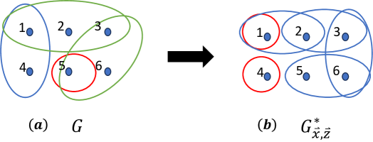
Figure 1: (a) A hypergraph with six vertices. We use big circles to label hyperedges and small points to label vertices. There are four hyperedges, $\{1,2,3\},\{3,5,6\},\{1,4\},\{5\}$, and the first two of them are $3$-edge. (b) shows the induced hypergraph $G^{*}_{\vec{x},\vec{z}}$ according to Eq. (11) and (12). Here two 6-bit strings are chosen as $\vec{x}=\{1,0,1,0,1,0\}$ and $\vec{z}=\{1,0,0,1,0,0\}$. For example, the 2-edge $\{1,2\}$ is induced from the $3$-edge $\{1,2,3\}$ of $G$ in (a) with $x_{3}=1$, according to the edge set $E^{(2)}_{\vec{x}}$ in Eq. (11); the 1-edge $\{4\}$ is directly by $z_{4}=1$ according to $E^{(1)}_{\vec{z}}$ in Eq. (12).

The following result relates the PL-component of any hypergraph state to the induced phase unitary.

Proposition 1.

Given a hypergraph state $\ket{G}$, the square of the PL-component respective to the Pauli operator $P_{\vec{x},\vec{z}}$ shows

$$\Tr{P_{\vec{x},\vec{z}}\ket{G}\bra{G}}^{2}=2^{-2n}\Tr{U(G_{\vec{x},\vec{z}})}^{2},$$ (13)

where $U(G_{\vec{x},\vec{z}})$ is the phase unitary determined by the hypergraph $G_{\vec{x},\vec{z}}$ defined in Eq. (11), which is induced from $G$ by the index vectors of $P_{\vec{x},\vec{z}}$.

The proof is left in Appendix A.2. By applying the above result of Eq. (13) to the definition of Eq. (9) and (10) and some further simplification, one has the following general formula for the magic of quantum hypergraph states.

Theorem 1.

The $\alpha$-order PL-moment of a hypergraph state $\ket{G}$ shows

$$\mathbf{m}_{\alpha}(\ket{G})=2^{-n(1+2\alpha)}\sum_{\vec{x},\vec{z}}\Tr{U(G^{*}_{\vec{x},\vec{z}})}^{2\alpha},$$ (14)

where $U(G^{*}_{\vec{x},\vec{z}})$ is the phase unitary determined by the hypergraph $G^{*}_{\vec{x},\vec{z}}$ defined in Eq. (12). The corresponding S$\textrm{R}_{\alpha}$E reads

$$\mathbf{M}_{\alpha}(\ket{G})=\frac{1+2\alpha}{\alpha-1}n+\frac{1}{1-\alpha}\log\sum_{\vec{x},\vec{z}}\Tr{U(G^{*}_{\vec{x},\vec{z}})}^{2\alpha}.$$ (15)

Compared to Eq. (13) with the phase unitary $U(G_{\vec{x},\vec{z}})$, Eq. (14) and (15) are only related to simplified one $U(G^{*}_{\vec{x},\vec{z}})$. This is based on the fact that the summation over all possible $\vec{z}$ simplifies the summation over all possible $E^{(1)}_{\vec{x},\vec{z}}$ to the one over $E^{(1)}_{\vec{z}}$. We remark that Ref. [50] also studied the magic of quantum hypergraph states mainly using the measure named min-relative entropy $\mathbf{D}_{\mathrm{min}}(\ket{G})$, which is related to the maximal fidelity to stabilizer states. In particular, they relate an upper bound of $\mathbf{D}_{\mathrm{min}}(\ket{G})$ to a minimization procedure of the nonquadraticity of the resulting Boolean function. However, the minimization result can only be obtained for a few example states. On the other hand, $\mathbf{M}_{\alpha}(\ket{G})$ shown here can be used as an lower bound of $\mathbf{D}_{\mathrm{min}}(\ket{G})$ [41, 51].

Theorem 1 transforms the PL-moment and also SRE into the calculation of trace of a family of phase unitary. There are totally $4^{n}$ such kind of induced $U(G^{*}_{\vec{x},\vec{z}})$, which makes the calculation of the magic for a given hypergraph state still challenging.

Specifically, for $3$-uniform hypergraph states $\ket{G_{n,3}}$, the hyperedges in $E^{(2)}_{\vec{x}}$ are all $2$-edges so the corresponding gates are $CZ$ gates. Then PL-moment in Eq. (14) becomes a summation of Boolean functions, for $\alpha=2$, it reads explicitly as

$$\mathbf{m}_{2}(\ket{G_{n,3}})=2^{-5n}\sum_{\vec{x},\vec{z}}\left(\sum_{\vec{a}}(-1)^{\sum_{i}z_{i}a_{i}+\sum_{j,k}b_{j,k}(\vec{x})a_{j}a_{k}}\right)^{4}$$ (16)

where $b_{j,k}(\vec{x})=\sum_{\{v_{i},v_{j},v_{k}\}\in E}x_{i}$ represents the summation of all the possible $CZ$ gates for a fix qubit-pair $\{j,k\}$. Naively, there are totally $8^{n}$ terms to sum the indices of $\vec{x},\vec{z}$ and also $\vec{a}$, which looks very sophisticated.

Nevertheless, based on the pictural expression in Theorem 1, we can give an upper bound of SRE of general hypergraph states with respect to its average degree.

Theorem 2.

For any $n$-qubit hypergraph state $\ket{G}$ whose corresponding graph $G$ has average degree $\bar{\Delta}(G)$, its S$R_{\alpha}$E with $\alpha\geq 2$ is upper bounded by

$$\mathbf{M}_{\alpha}(\ket{G})\leq\frac{1}{\alpha-1}\left[1-\log\left(1+\frac{1}{2^{(2\alpha-1)\bar{\Delta}(G)}}\right)\right]n.$$ (17)

The proof is left in Appendix B. For $\alpha=2$, and a large enough $\bar{\Delta}(G)$, the upper bound in Eq. (17) behaves like $[1-\log(e)^{-1}2^{-3\bar{\Delta}(G)}]n$. This indicates that for a quantum hypergraph state with $\bar{\Delta}(G)$ bounded by some constant, its magic cannot reach the maximum possible value $n-o(n)$. This bound especially constrains the magic of hypergraph states on the lattice.

IV Magic of random hypergraph states

In this section, we study the statistical properties magic of random hypergraph states. First, we define some random hypergraph state ensembles $\mathcal{E}$ from the corresponding random hypergraph ensembles. Here, we mainly study random $c$-uniform hypergraphs, which only own $c$-edge. A random $c$-uniform hypergraph ensemble can be determined by the probability $p$ whether there is a $c$-edge or not among all choices of $c$ vertices. Denote the combination number $C^{c}_{n}:=\binom{n}{c}$, and the ensembles are defined formally as follows [67].

Definition 3.

The ($c$-uniform) random hypergraph state ensemble $\mathcal{E}_{c}^{p}$ of $n$-qubit system is defined as

$$\mathcal{E}_{c}^{p}=\left\{\ket{\Psi}=U\ket{\Psi_{0}}\Big{|}U=U_{e_{C_{n}^{c}}}\cdots U_{e_{2}}U_{e_{1}}\right\}.$$ (18)

Here each $e_{i}$ is a distinct $c$-edge of the $n$ vertices, with totally $C^{c}_{n}$ such edges, $U_{e_{i}}$ acts on the Hilbert space $\mathcal{H}_{e_{i}}$ by taking $\{\mathbb{I}_{e_{i}},CZ_{e_{i}}\}$ from the probability distribution $\{1-p,p\}$ respectively, and the initial state $\ket{\Psi_{0}}=\ket{+}^{\otimes N}$.

Note that the specific gate sequence in Eq. (18) is not relevant, as $CZ_{e}$ gates commute with each other. In particular, as $p=1/2$, all the elements in $\mathcal{E}_{k}$ share an equal probability $1/|\mathcal{E}_{c}|$ with $|\mathcal{E}_{c}|=2^{C_{n}^{c}}$ [67]. Hereafter we omit the superscript $p$ of $\mathcal{E}_{c}^{p}$ as $p=1/2$ for simplicity of notation. See Fig. 2 (a) for an example of a $3$-uniform hypergraph state.

The SRE defined in Eq. (10) is in the logarithmic function. As such, to analyze the average property of SRE for some state ensembles $\mathcal{E}$, we instead focus on the calculation of the average PL-moment of Eq. (9) inside the logarithm, that is,

$$\langle\mathbf{m}_{\alpha}\rangle_{\mathcal{E}}=\mathbb{E}_{\Psi\in\mathcal{E}}[\mathbf{m}_{\alpha}(\ket{\Psi})].$$ (19)

This directly gives a lower bound of the S$\textrm{R}_{\alpha}$E by the concavity of the logarithmic function.

$$\langle\mathbf{M}_{\alpha}\rangle_{{\mathcal{E}}}\geq(1-\alpha)^{-1}\log\langle\mathbf{m}_{\alpha}\rangle_{\mathcal{E}}.$$ (20)

for $\alpha>1$.

In particular, for $p=1/2$, one has the average PL-moment of the hypergraph ensemble $\mathcal{E}_{c}$ defined in Eq. (18) as

$$\langle\mathbf{m}_{\alpha}\rangle_{\mathcal{E}_{c}}=|\mathcal{E}_{c}|^{-1}\sum_{G_{n,c}\in\mathcal{G}_{n,c}}\mathbf{m}_{\alpha}(\ket{G_{n,c}}),$$ (21)

where $\mathcal{G}_{n,c}=\{G\big{|}|V|=n,\forall e\in E,|e|=c\}$ is the set of $c$-uniform hypergraphs.

Hereafter we focus on $\alpha\geq 2\in\mathbb{Z}$ and the uniform ensemble $\mathcal{E}_{c}$ to calculate the average properties and the fluctuations of the magic, and then extend to non-uniform ensemble $\mathcal{E}_{c}^{p}$ later. The adjustment of the probability parameter $p$ can thus change the expected density of the applied gates and also the expected average degree of the corresponding hypergraph, which is discussed in Sec. IV.3. We remark that our work is the first to show statistical properties of magic for some realistic ensembles beyond Haar random states [41, 21, 62].

IV.1 Average analysis of magic

In this section, our main focus is on the average properties of magic, especially the PL-moment, and then we show quite tight lower bounds of the average SRE. The following theorem transforms the average PL-moment into a counting problem of binary strings. We first show some related definitions of the norm and operations of an $n$-bit string $\vec{t}=\{t^{i}\}$. The $1$-norm $\norm{\vec{t}}_{1}=\sum_{i}t^{i}$, with the addition modulo $2$. The Hadamard or Schur product $\bigodot$ of some bit strings $\vec{t_{k}}$ is the element-wise product, i.e., $\vec{t^{\prime}}=\bigodot_{k}\vec{t_{k}}$ with ${t^{\prime}}^{i}=\prod_{k}t_{k}^{i}$.

Theorem 3.

For any integer $\alpha\geq 2\in\mathbb{Z}$, the average $\alpha$-th PL-moment of $n$-qubit random hypergraph state ensembles $\mathcal{E}_{c}$ defined in Eq. (18) shows

$$\langle\mathbf{m}_{\alpha}\rangle_{\mathcal{E}_{c}}=\frac{\mathrm{N}(c,\alpha,n)}{2^{2\alpha n}}$$ (22)

where $\mathrm{N}(c,\alpha,n)$ is the number of $2$-tuple $(\mathrm{T},\vec{x})$, such that the following two constraints are satisfied.

$$\norm{\vec{t_{i}}}_{1}=0,\quad\forall i,$$ (23)

$$\sum_{q\subset e_{c}}\left(\prod_{v_{i}\in q}x_{i}\norm{\bigodot_{v_{k}\in e_{c}\setminus q}\vec{t_{k}}}_{1}\right)=0,\quad\forall|e_{c}|=c,$$ (24)

where $\mathrm{T}=(\vec{t_{1}},\cdots,\vec{t_{i}},\cdots,\vec{t_{n}})$ is a $2\alpha\times n$ binary matrix, $\vec{x}$ is an $n$-bit vector with elements $x_{i}$, and $e_{c}$ labels all possible $c$-edges.

The full proof is left in Appendix C.1, and here we give some intuition about the proof. We mainly utilize the replica trick to write the average PL-moment on $2\alpha$-copy of the original Hilbert space $\mathcal{H}_{d}^{\otimes 2\alpha}$ [41, 49, 67]. Consequently, the computational basis of every qubit can be labeled by a $2\alpha$-bit string [67], i.e., $\vec{t_{i}}$ of the matrix $\mathrm{T}$ for the $i$-th qubit. The two constraints Eq. (23) and Eq. (24), which look a bit complicated at first glance, actually correspond to the induced hypergraph structure of Eq. (12) previously introduced in Sec. III. In particular, the first constraint Eq. (23) accounts for the effect of the expectation from $2\alpha$-replica on the edge set $E^{(1)}_{\vec{z}}$, and the second one Eq. (24) for the edge set $E^{(2)}_{\vec{x}}$, that is, edges introducing multi-qubit controlled gates. See Fig. 2 (b) for an illustration of the constraints when $c=3$ and $\alpha=2$.

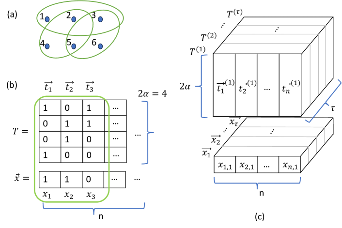
Figure 2: (a) A random $c=3$-unifrom hypergraph with 6 vertices. In this case, there are three $3$-edges selected, $\{1,2,3\},\{2,4,5\},\{3,5,6\}$. The ensemble $\mathcal{E}_{c}^{p}$ in Def. 3 contains random hypergraph states, whose hypergraphs are generated by selecting all possible $c$-edges independently with probability $p$. (b) An illustration of the constraints in Thereom 3 and Corollary 2 with $c=3$ and $\alpha=2$. Here we explicitly give the first three 4-bit stings $\vec{t_{1}},\vec{t_{2}},\vec{t_{3}}$ with respective to the first three qubits, and clearly they satisfy the parity constraint in Eq. (23). The second constraint in Eq. (24) is simplified to Eq. (28) as $c=3$. For a specific $3$-edge $e_{3}=\{1,2,3\}$, its induced constraint reads $x_{1}\norm{\vec{t_{2}}\bigodot\vec{t_{3}}}_{1}+x_{2}\norm{\vec{t_{3}}\bigodot\vec{t_{1}}}_{1}+x_{3}\norm{\vec{t_{1}}\bigodot\vec{t_{2}}}_{1}=0$, and it is satisfied if $\vec{x}=\{1,1,0,\cdots\}$. Note that the assignment of $\mathrm{T}=\{\vec{t_{i}}\}_{i=1}^{n}$ and $\vec{x}$ should satisfy all such constraint from every $3$-edge. (c) A graphic illustration of the 2-tuple $(\mathcal{T},\mathrm{X})$ in Thereom 4. $\mathcal{T}$ is a $2\alpha\times n\times\tau$ $3$-order tensor, and $\mathrm{X}$ is a $n\times\tau$ matrix. The first constraint in Eq. (32) is just the parity one for each $\vec{t_{i}}^{(s)}$ of $\mathcal{T}$. The second one in Eq. (33) is a generalization of Eq. (24), by additionally summing the index $s\in[\tau]$. For every edge $e_{c}$, one first calculates Eq. (24) on each plane of this cube and then sums all of them in the longitudinal direction.

Before showing refined results later, we first give some preliminary estimation of the counting problem in Theorem 3. Note that Eq. (23) is indeed the parity constraint and independent of $\vec{x}$. Denote the set $\mathcal{D}=\left\{\vec{t}~{}\big{|}~{}\|\vec{t}\|_{1}=0\right\}$ of $2\alpha$-bit strings as the valid set, one directly has $|\mathcal{D}|=2^{2\alpha-1}$. Each $\vec{t_{i}}$ of $\mathrm{T}$ should be taken from $\mathcal{D}$, and consequently the entire matrix $\mathrm{T}$ comprises $\left(2^{2\alpha-1}\right)^{n}$ alternatives when Eq. (23) satisfied. Furthermore, as for Eq. (24), one needs to find the number of $\vec{x}$ given a specific assignment of $\mathrm{T}$ with each $\vec{t_{i}}\in\mathcal{D}$. Supposed that $\vec{x}=\vec{0}$, it is not hard to check that in this case, Eq. (24) induces no constraint on $\mathrm{T}$. If we ignore the constraint of Eq. (24), it is clear that there are totally $2^{n}$ distinct $\vec{x}$. On account of these observations, we have a lower bound and a trivial upper bound of PL-moment as

$$\frac{(2^{2\alpha-1})^{n}\cdot 1}{2^{2\alpha n}}=2^{-n}\leq\langle\mathbf{m}_{\alpha}\rangle_{\mathcal{E}_{c}}\leq\frac{(2^{2\alpha-1})^{n}\cdot 2^{n}}{2^{2\alpha n}}=1.$$ (25)

The upper bound is just $1$ and is trivial by definition of moments. With a refined analysis of Eq. (24) and more exact counting of $\mathrm{N}(c,\alpha,n)$, a non-trivial upper bound of the PL-moment is shown as follows for general $\alpha$ and $c$.

Proposition 2.

For any $c\geq 3\in\mathbb{Z}$ and $\alpha\geq 2\in\mathbb{Z}$, with the qubit number $n\gg\alpha$ and $n\gg c$, the average PL-moment

$$\langle\mathbf{m}_{\alpha}\rangle_{\mathcal{E}_{c}}\leq\frac{2^{(c+2^{2\alpha-2})}}{2^{n}}.$$ (26)

In particular, for $c=3$ and $\alpha=2$, it shows $\langle\mathbf{m}_{2}\rangle_{\mathcal{E}_{3}}\leq 2^{-(n-7)}$.

The upper bound in Proposition 2 is a bit loose considering the dependence on the parameters $c$ and $\alpha$, which is exponential to $c$ and even double-exponential to $\alpha$. However, suppose one only considers constant $c$ and $\alpha$ and focuses on the relation to the qubit number $n$, the upper bound then shows $\langle\mathbf{m}_{\alpha}\rangle_{\mathcal{E}_{c}}=O\left(2^{-n}\right)$, which matches the lower bound in Eq. (25). We summarize this and its implication to SRE via Eq. (20) in the following corollary.

Corollary 1.

For any $c\geq 3\in\mathbb{Z}$ and $\alpha\geq 2\in\mathbb{Z}$, with $n\gg\alpha$ and $n\gg c$, the average SRE is lower bounded by

$$\langle\mathbf{M}_{\alpha}\rangle_{\mathcal{E}_{c}}\geq(\alpha-1)^{-1}[n-(c+2^{2\alpha-2})].$$ (27)

In particular, for constant $c$ and $\alpha$, it shows that $\langle\mathbf{M}_{\alpha}\rangle_{\mathcal{E}_{c}}\geq(\alpha-1)^{-1}n-O(1)$.

Note that as $\alpha=2$, the lower bound of average SRE shows that the magic of random hypergraph states is nearly the maximal possible value $n$ for any constant $c\geq 3$ and sufficiently large qubit number $n$, which reproduces the result of Haar random states [41].

Furthermore, a more refined analysis can be conducted when focusing on $3$-uniform hypergraph states. A direct simplification of Eq. (24) in this case is shown as follows.

Corollary 2.

As $c=3$, the second constraint in Eq. (24) of Theorem 3 can be simplified to

$$\begin{gathered}\sum_{v_{i}\in e_{3}}\left(x_{i}\norm{\bigodot_{k\neq i,v_{k}\in e_{3}}\vec{t_{k}}}_{1}\right)=0,\quad\forall|e_{3}|=3.\end{gathered}$$ (28)

The proof is straightforward. As $c=3$, one only needs to sum over all possible $q$ with $|q|=1$ and $|q|=2$ in Eq. (24). For $|q|=2$, the set $e_{3}\setminus q$ only has one element, so the $l_{1}$-norm is just for a single binary vector, which is already constrained by Eq. (23). As a result, the constraint is reduced to that for $|q|=1$ as shown in Eq. (28). Based on this simplification, we give the following more accurate counting results.

Proposition 3.

The average PL-moments of random $3$-uniform hypergraph states are

$$\langle\mathbf{m}_{2}\rangle_{\mathcal{E}_{3}}=\frac{7}{2^{n}}-\frac{14}{4^{n}}+\frac{8}{8^{n}},$$ (29)

$$\langle\mathbf{m}_{\alpha}\rangle_{\mathcal{E}_{3}}\leq\frac{4}{2^{n}}+\frac{(2\alpha-1)!!}{2^{(\alpha-1)n}},\quad\forall\alpha\geq 3\in\mathbb{Z}.$$

The proofs of Propositions 2 and 3 are left in Appendix C.3 and D.1, respectively.

IV.2 Variance analysis of magic

In this section, we further investigate the variance of PL-moments, which is helpful in constructing a sharp concentration result of SRE for random hypergraph states in the large $n$ limit. In this way, we find that hypergraph states which are easier to prepare, typically own the maximal magic, similar to the Haar random states.

The variance of PL-moment is defined as

$$\delta^{2}_{\mathcal{E}}[\mathbf{m}_{\alpha}] :=\langle\mathbf{m}_{\alpha}^{2}\rangle_{\mathcal{E}}-\langle\mathbf{m}_{\alpha}\rangle_{\mathcal{E}}^{2}$$ (30)

with the average PL-moment $\langle\mathbf{m}_{\alpha}\rangle_{\mathcal{E}}$ given in Eq. (19). The average PL-moment is investigated in the previous Sec. IV.1, and hereafter we focus on the analysis of the first term, i.e., the average of the $2$-th moment of the PL-moment, and then combine them to show the final variance.

As an analog and extension of Theorem 3, for the general $\tau$-th moment of the PL-moment, we transform the calculation of its average on random hypergraph state ensembles into the following counting problem.

Theorem 4.

For any integer $\alpha\geq 2\in\mathbb{Z}$, the $\tau$-th moment of the $\alpha$-th PL-moment of $n$ qubit random hypergraph state ensembles $\mathcal{E}_{c}$ shows

$$\langle\mathbf{m}_{\alpha}^{\tau}\rangle_{\mathcal{E}_{c}}=\frac{\mathrm{N}^{(\tau)}(c,\alpha,n)}{2^{2\tau\alpha n}}$$ (31)

where $\mathrm{N}^{(\tau)}(c,\alpha,n)$ is the number of $2$-tuple $(\mathcal{T},\mathrm{X})$, such that the following two constraints are satisfied.

$$\norm{\vec{t_{i}}^{(s)}}_{1}=0,\quad\forall i,s$$ (32)

$$\sum_{s=1}^{\tau}\sum_{q\subset e_{c}}\left(\prod_{v_{i,s}\in q}x_{i,s}\norm{\bigodot_{v_{k}\in e_{c}\setminus q}\vec{t_{k}}^{(s)}}_{1}\right)=0,\quad\forall|e_{c}|=c,$$ (33)

where $\mathcal{T}$ is a $2\alpha\times n\times\tau$ rank-$3$ binary tensor, with its element $2\alpha\times n$ matrix denoted by $\mathrm{T}^{(s)}=({\vec{t_{1}}}^{(s)},\cdots,\vec{t_{i}}^{(s)},\cdots,\vec{t}^{(s)}_{n})$ for $s\in[\tau]$, and the element of the $i$-th binary vector $\vec{t_{i}}^{(s)}$ is $t^{(s)}_{j,i}$; $\mathrm{X}=(\vec{x_{1}},\cdots,\vec{x_{s}},\cdots,\vec{x_{\tau}})$ is an $n\times\tau$ binary matrix with elements $x_{i,s}$.

Note that Theorem 4 reduces to Theorem 3 as $\tau=1$, and its proof is similar but more complicated, which is left in Appendix C.2. The counting problem here is more challenging even for $\tau=2$ of interest, compared to the one in Theorem 3 of Sec. IV.1. Instead of showing a general result similar to Proposition 2, we focus on the case where $\alpha=2$ and $c=3$ here and further give an upper bound for the variance of the PL-moment.

Proposition 4.

The variance of $2$-order PL-moment on the random $3$-uniform hypergraph state ensemble $\mathcal{E}_{3}$ is

$$\delta^{2}_{\mathcal{E}_{3}}[\mathbf{m}_{2}]=\langle\mathbf{m}_{2}^{2}\rangle_{\mathcal{E}_{3}}-\langle\mathbf{m}_{2}\rangle_{\mathcal{E}_{3}}^{2}\leq\frac{37}{2^{3n}}.$$ (34)

The proof is by estimating the counting result in Theorem 4 for $\tau=2,\alpha=2$ and $c=3$, and then combining with $\langle\mathbf{m}_{2}\rangle_{\mathcal{E}_{3}}$ in Eq. (29), and we leave it in Appendix D.2. Note that the standard variance here $\delta_{\mathcal{E}_{3}}[\mathbf{m}_{2}]=O(2^{-1.5n})$ is exponentially small than its mean value $\langle\mathbf{m}_{\alpha}\rangle_{\mathcal{E}_{3}}=O(2^{-n})$ as shown in Eq. (29). Consequently, by utilizing Chebyshev’s inequality, there is the concentration of measure effect of magic for the $\mathcal{E}_{3}$ ensemble.

Corollary 3.

For a hypergraph state $\ket{G_{n,3}}$ of $n$-qubit chosen randomly from the $3$-unifrom hypergraph state ensemble $\mathcal{E}_{3}$, the probability that its S$\textrm{R}_{2}$E larger than $n-3$ is almost $1$, that is

$$\Pr\left\{\mathbf{M}_{2}(\ket{G_{n,3}})\geq n-3\right\}\geq 1-\frac{37}{2^{n}}.$$ (35)

A similar concentration effect of magic is also observed for Haar random states [41, 21, 62]. However, compared with Haar random states, $\mathcal{E}_{3}$ are quite easy to prepare, i.e., just by randomly operating three-qubit $CCZ$ gates.

IV.3 Average magic with general probability $p$

In the previous two subsections, Sec. IV.1 and Sec. IV.2, we mainly focus on the magic properties of the hypergraph state ensemble $\mathcal{E}_{c}$. In this section, we extend the ensemble $\mathcal{E}_{c}$ to $\mathcal{E}_{c}^{p}$ in Definition 3, where each $c$-edge is randomly selected by the probability parameter $p$. In particular, we focus on the $c=3$ and $\alpha=2$ cases and show the following analytical formula for the average PL-moment for any $n$-qubit system.

Theorem 5.

The average $2$-order PL-moment of the state ensemble $\mathcal{E}_{3}^{p}$, i.e., random $3$-uniform hypergraph state with each hyperedge selected by probability $p$, shows

$$\langle\mathbf{m}_{2}\rangle_{\mathcal{E}_{3}^{p}}=2^{-3n}\sum_{\vec{\kappa}}{n\choose\vec{\kappa}}(1-2p)^{f(\vec{\vec{\kappa}})}.$$ (36)

Here $\vec{\kappa}=\left(\vec{\kappa^{+}},\vec{\kappa^{-}}\right)$ is a $8$-dimension vector composed of two $4$-dimension vectors $\vec{\kappa^{+}}$ and $\vec{\kappa^{-}}$, with each element $\kappa^{\pm}_{1\leq i\leq 4}\in\mathbb{N}$ being non-negative integer; the summation of the elements of $\vec{\kappa}$ equals $\sum_{i=1}^{4}(\kappa_{i}^{+}+\kappa_{i}^{-})=n$, and the multinomial coefficient ${n\choose\vec{\kappa}}$ is short for the combinatorial number ${n\choose\kappa_{0}^{+},\kappa_{0}^{-},\kappa_{1}^{+},\kappa_{1}^{-},\kappa_{2}^{+},\kappa_{2}^{-},\kappa_{3}^{+},\kappa_{3}^{-}}$; the function reads

$$f(\vec{\kappa})= \kappa_{0}^{+}(\kappa_{1}\kappa_{2}+\kappa_{2}\kappa_{3}+\kappa_{3}\kappa_{1})$$ (37)

$$+\kappa_{1}^{+}\kappa_{1}^{-}(\kappa_{2}+\kappa_{3})+\kappa_{2}^{+}\kappa_{2}^{-}(\kappa_{3}+\kappa_{1})+\kappa_{3}^{+}\kappa_{3}^{-}(\kappa_{1}+\kappa_{2})$$

$$+\kappa_{1}^{+}\kappa_{2}^{-}\kappa_{3}^{-}+\kappa_{2}^{+}\kappa_{3}^{-}\kappa_{1}^{-}+\kappa_{3}^{+}\kappa_{1}^{-}\kappa_{2}^{-}+\kappa_{1}^{+}\kappa_{2}^{+}\kappa_{3}^{+}$$

with $\kappa_{i}=\kappa_{i}^{+}+\kappa_{i}^{-}$ for short.

The proof is left in Appendix E. We remark that Theorem 5 could be extended to arbitrary constant $c$ cases while the polynomial complexity of calculation holds since one still only needs to sum over some combinatorial number of the vector $\vec{\kappa}$.

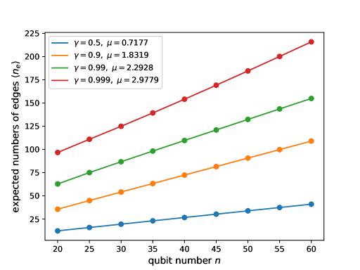
Figure 3: Relation between qubit number $n$ ($x$-axis) and expected number of hyperedges $\langle n_{e}\rangle=p\cdot{n\choose 3}$ ($y$-axis), given the (lower bound of) expected S$\textrm{R}_{2}$E $\underline{\langle\mathbf{M}_{2}\rangle_{\mathcal{E}_{3}^{p}}}=-\log\langle\mathbf{m}_{2}\rangle_{\mathcal{E}_{3}^{p}}=\gamma\cdot n$ for different $\gamma$’s. Different colors represent different expected magic with different slopes $\mu$’s.

Note that Eq. (29) of the previous $p=1/2$ case is obtained by counting the number of solutions to $f(\vec{\vec{\kappa}})=0$. For the general $p$ here, we do not have a very compact formula, and the function $f(\vec{\vec{\kappa}})$ and also $\langle\mathbf{m}_{2}\rangle_{\mathcal{E}_{3}^{p}}$ in Eq. (36) look a little tedious. Nevertheless, the calculation of $\langle\mathbf{m}_{2}\rangle_{\mathcal{E}_{3}^{p}}$ only involves polynomial complexity with respective to the qubit-number $n$, that is, $O(n^{7}\log n)$. This fact enables us to numerically study the relationship between the average magic and the probability $p$ for quite large $n$, as shown in Fig. 3.

To be specific, Fig. 3 shows the relation between the expected number of hyperedges $\langle n_{e}\rangle:=p\cdot{n\choose 3}$ and the qubit-number $n$, given the average magic $\langle\mathbf{m}_{2}\rangle_{\mathcal{E}_{3}^{p}}=\gamma n$ for some constant $\gamma$. One can see that for a fixed proportion $\gamma$ of $n$, $\langle n_{e}\rangle$ is almost linear to $n$ for different $\gamma$’s, i.e., $\langle n_{e}\rangle\sim\mu n$, and thus $p\sim O(n^{-2})$ far less than $1/2$ like before.

For each vertex, the expected number of edges is

$$\langle n_{e}\rangle\cdot\frac{{n-1\choose 2}}{{n\choose 3}}\sim 3\mu,$$ (38)

and thus the expected average degree $\langle\bar{\Delta}(G)\rangle$ is about a constant. This shows the consistency to Theorem 2, where the magic of a bounded-average-degree hypergraph state is also bounded. For $\gamma=0.999$, which is very near the maximal $1$, the slope $\mu\simeq 3.0$. It means that a very small $p$ can let the average magic near the maximal value.

The statistical results here may also suggest a dynamical way to generate maximal magic states efficiently. For each step, one operates a $CCZ$ gate on any three-qubit chosen randomly from a $3$-edge, and repeats this process for about $K=O(n)$ times. In particular, the numerical result implies that $K=3n$ may be enough to let S$\textrm{R}_{2}$E reach $0.999n$. Moreover, if one parallel applies $CCZ$ gates, constant-depth (depth-$3\mu$) quantum circuit could be sufficient (depth-9 for $\mathbf{M}_{2}(\ket{G})\sim 0.999n$).

V Magic of some symmetric hypergraph states

In this section, we investigate the magic of some hypergraph states with permutation symmetry. We focus on the $c$-complete hypergraph states with $c=3$ and $c=n$, and our method can be applied to other symmetric hypergraph states.

The motivation for this study is two-fold. First, for any $c$-complete hypergraph, every vertex is connected to other $n-1$ vertices, and thus the average degree being $\bar{\Delta}(G_{c\textrm{-com}})=n-1$. Consequently, $c$-complete hypergraph states can give some new insight beyond the one with a bounded average degree whose magic is constrained by Theorem 2. Second, the permutation symmetry significantly simplifies the summation of indices ${\vec{x},\vec{z}}$ in Eq. (14) from exponential to polynomial. This fact and the pictural magic formula introduced in Theorem 1 enable calculating the spectrum of the PL-components, and thus S$\textrm{R}_{\alpha}$E for any $\alpha$. In particular, $\alpha$ needs not to be limited to integers as that in Sec. IV, for instance, here one can take $\alpha=1/2$.

Definition 4.

An $n$-partite quantum state $\ket{\Psi}$ owns permutation symmetry, if

$$U_{\{\pi\}}\ket{\Psi}\bra{\Psi}U^{\dagger}_{\{\pi\}}=\ket{\Psi}\bra{\Psi},\ \forall\pi\in S_{n}.$$ (39)

Here $\pi$ is the permutation element in the $n$-th order symmetric group $S_{n}$. $U_{\{\pi\}}$ is an unitary representation with $U_{\{\pi\}}\ket{a_{1},a_{2},\cdots,a_{n}}=\ket{a_{\pi(1)},a_{\pi(2)},\cdots,a_{\pi(n)}}$ with $\{\ket{a}\}$ the basis state for a single-party. For example, $U_{\{(1,2)\}}$ is the swap operator on 2-party.

Due to the permutation symmetry, the PL-component $\Tr{P_{\vec{x},\vec{z}}\ket{\Psi}\bra{\Psi}}$ is not relevant to the specific positions of single-qubit Pauli operators but only depends on the numbers of them, i.e., $x_{i}=1$ and $z_{i}=1$ and both $x_{i}=z_{i}=1$ in $P_{\vec{x},\vec{z}}$. Denote the corresponding sets of $P_{\vec{x},\vec{z}}$ as $A_{x}=\{i|x_{i}=1\}$, $A_{-x}=\{i|x_{i}=0\}$, $A_{z,x}=\{i|z_{i}=1,x_{i}=1\}$, $A_{z,-x}=\{i|z_{i}=1,x_{i}=0\}$, one has the following general observation.

Observation 2.

For an $n$-partite quantum state $\ket{\Psi}$ owning permutation symmetry defined in Def. 4, its PL-component $\Tr{P_{\vec{x},\vec{z}}\ket{\Psi}\bra{\Psi}}$ is directly related to the cardinality of the sets $m=|A_{x}|$, $m_{1}=|A_{z,x}|$ and $m_{0}=|A_{z,-x}|$, but not the specific positions. That is, two components take the same value if these sets share the same cardinality.

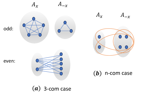
Figure 4: Illustration of induced hypergraphs for $c$-complete hypergraph states. Here the shaded areas label the corresponding sets. Due to the permutation symmetry, the induced hypergraph $G^{*}_{\vec{x},\vec{z}}$ defined in Eq. (11) and (12) is determined by $|A_{x}|$, $|A_{z,x}|$ and $|A_{z,-x}|$. Since $E^{(1)}_{\vec{z}}$ in Eq. (12) only introduces 1-edges, for simplicity, we take $\vec{z}=0$ and thus $|A_{z,x}|=|A_{z,-x}|=0$. In this way, the structure of $G^{*}_{\vec{x},\vec{0}}$ only depends on $m=|A_{x}|$. (a) $3$-complete hypergraph with 8 vertices: $G^{*}_{\vec{x},\vec{0}}$ is related to even/odd of $m$, and it is either two complete-graphs of $A_{x}$ and $A_{-x}$ or complete bipartite graph between them. (b) $n$-complete hypergraph with 6 vertices with $m=2$: $G^{*}_{\vec{x},\vec{0}}$ in this case contains all the hyperedges $A_{-x}\subseteq e^{\prime}\subset V$. See Appendix F for more detailed discussions.

For quantum hypergraph states whose PL-component is proportional to $\Tr{U(G_{\vec{x},\vec{z}})}$ as shown in Proposition 1, if they own permutation symmetry, like $c$-complete hypergraph states, the induced hypergraphs $G_{\vec{x},\vec{z}}$ (and also $G^{*}_{\vec{x},\vec{z}}$) are isomorphic to each other if the aforementioned sets share the same cardinality. This observation and the pictural magic formula in Theorem 1 make the calculations intuitive and elegant.

In the following, we first show the results of magic for $3$- and $n$-complete hypergraph states, respectively, and then give a series of comments on them. We leave the detailed proofs in Appendix F. We show their induced hypergraphs $G^{*}_{\vec{x},\vec{z}}$ in Fig. 4.

Proposition 5.

The $2$-order and $1/2$-order PL-moment of the quantum $3$-complete hypergraph state of $n$-qubit $\ket{G_{3\textrm{-com}}}$ are

$$\mathbf{m}_{2}(\ket{G_{3\textrm{-com}}})=\frac{1}{8}+\frac{7}{2^{n+\frac{3-(-1)^{n}}{2}}},$$ (40)

$$\mathbf{m}_{1/2}(\ket{G_{3\textrm{-com}}})=2^{\frac{2n-7-(-1)^{n}}{4}}+1-2^{-n+\frac{1+(-1)^{n}}{2}}.$$

Consequently, the corresponding $SRE$ approaches $\mathbf{M}_{2}(\ket{G_{3\textrm{-com}}})\rightarrow 3$ and $\mathbf{M}_{1/2}(\ket{G_{3\textrm{-com}}})\rightarrow n-\frac{7+(-1)^{n}}{2}$, as $n\rightarrow\infty$.

Proposition 6.

The $2$-order and $1/2$-order PL-moment of the quantum $n$-complete hypergraph state of $n$-qubit $\ket{G_{n\textrm{-com}}}$ are

$$\mathbf{m}_{2}(\ket{G_{n\textrm{-com}}})=1-16\cdot 2^{-n}+112\cdot 2^{-2n}$$ (41)

$$\ \ \ \ \ \ \ \ \ \ \ \ \ \ \ \ \ \ \ \ -224\cdot 2^{-3n}+128\cdot 2^{-4n},$$

$$\mathbf{m}_{1/2}(\ket{G_{n\textrm{-com}}})=3-10\cdot 2^{-n}+8\cdot 2^{-2n}.$$

for $n\geq 2$. Consequently, the corresponding SRE $\mathbf{M}_{2}(\ket{G_{n\textrm{-com}}})$ shows its maximal value $\log{\frac{32}{11}}\approx 1.54$ when $n=3$, and decreases exponentially with $n$; $\mathbf{M}_{1/2}(\ket{G_{n\textrm{-com}}})$ increases monotonously to $2\log_{2}{3}$ as $n\rightarrow\infty$.

First, these two examples indicate that hypergraph states with an unbounded average degree could not own maximum magic, opposite to Theorem 2. For $\ket{G_{3\textrm{-com}}}$, S$\textrm{R}_{\frac{1}{2}}$E is about a constant, even though there are extensive $CCZ$ gates to generate it. This phenomenon also appears in entanglement analysis, where over-connected graph and hypergraph states only own a small amount of entanglement. For instance, the $2$-complete graph state is equivalent to the GHZ state [64], with entanglement entropy being $1$ for any bipartition.

For $\ket{G_{n\textrm{-com}}}$, its S$\textrm{R}_{2}$E even scales like $O(2^{-n})$ for the large $n$ limit. This behavior can be understood via the fidelity to the initial stabilizer state $\ket{\Psi_{0}}$ with zero magic. The $n$-qubit gate $CZ_{n}$ is nearly an identity operator for a large $n$, and the fidelity $F(\ket{G_{n\textrm{-com}}},\ket{\Psi_{0}})=\bra{G_{n\textrm{-com}}}\Psi_{0}\rangle=1-2^{-n}$. As such, $G_{n\textrm{-com}}$ should have small magic as being close to a stabilizer state.

Second, the S$\textrm{R}_{2}$E and S$\textrm{R}_{\frac{1}{2}}$E are very different for both states. In particular, $\mathbf{M}_{1/2}(\ket{G_{3\textrm{-com}}})$ is near $n$, however, $\mathbf{M}_{2}(\ket{G_{3\textrm{-com}}})$ is about a constant. This is mainly due to the distribution of the PL-component of $\ket{G_{3\textrm{-com}}}$. There are almost half of PL-components are non-zero, but their distribution is very sharp. That is, most of them are extraordinarily small. and on the contrary, only a constant number of them are larger as $O(1)$. This phenomenon may lead to significant consequences in further one-shot manipulations [68, 69].

VI Conclusion and outlook

In this work, we study the magic properties of quantum hypergraph states in terms of SRE. We find that the random hypergraph states typically have near-maximal magic, indicating an efficient way to generate them by dynamically applying few-qubit controlled phase gates. We also show a general upper bound of magic by the degree of the corresponding hypergraph and give a few analytical solutions to states with permutation symmetry. The general pictural formula of magic presented here can advance further explorations of many-qubit magic for large-scale systems.

From the results shown here, there are several directions to investigate further. First, it is direct to generalize the current study to other phase diagonal states [70, 71, 72], especially those generated by 2-qubit $CZ_{\theta}$ gates. $CZ_{\theta}$ gate is more feasible in practise than $3$-qubit $CCZ$ gate and still can create magic. Second, the permutation symmetry significantly simplifies the calculation of magic, leading to a few analytical results, and it is promising to generalize to other states beyond hypergraph states, for example, the W-state [44]. It is thus interesting to analyze the statistical properties of state ensembles with high symmetry [73]. Third, there is a large gap of S$\textrm{R}_{\alpha}$E for different $\alpha$’s, and this indicates the significance of analyzing the spectrum of the PL-component, which may play an important role similar to the entanglement spectrum [74, 75, 76]. And the implications of this phenomenon to one-shot quantum resource theory [69] and magic distillation of many-qubit states [77] also deserve further studies. Finally, it is known that typically random hypergraph states also have near-maximal entanglement [67]. Thus the following important question arises—whether quantum states with near-maximal magic necessarily own a large amount of entanglement? The random states and permutation-symmetry states here give some positive support. Or, more broadly, what are the general relations and constraints between these two key quantum resources [26, 78]? The answers to these questions would definitely unveil some ultra-quantum features and benefit quantum information processing.

VII Acknowledgement

We thank Alioscia Hamma, Xiongfeng Ma, and Ryuji Takagi for their useful discussions. J. C and Y. Y acknowledge the support of the National Natural Science Foundation of China (NSFC) via Grant No. 12174216. Y. Z acknowledges the support of the NSFC via Grant No. 12205048 and the start-up funding of Fudan University.

Appendix A Related Proofs of the general formula of magic for hypergraph states

A.1 Proof of Observation 1

First, a quick observation shows that the stabilizer generator reads

$$S_{i} =U(G)X_{i}U^{{\dagger}}(G)=\prod_{e\in E}CZ_{e}\cdot X_{i}\cdot\prod_{e\in E}CZ_{e}$$ (42)

$$=X_{i}\cdot\prod_{e\in E}X_{i}CZ_{e}X_{i}\cdot\prod_{e\in E}CZ_{e}$$

$$=X_{i}\prod_{e\in E,e\ni v_{i}}CZ_{e\setminus\{v_{i}\}},$$

where in the second line we insert additional $X_{i}$ for each $CZ_{e}$ and apply the relation $X_{i}CZ_{e}X_{i}=CZ_{e}\cdot CZ_{e\setminus\{v_{i}\}}$. Note that $U^{{\dagger}}(G)=U(G)$ for phase gates considered in our work.

Then we prove that for any set $e^{\prime}\subseteq e$,

$$\left(\prod_{v_{i}\in e^{\prime}}X_{i}\right)CZ_{e}\left(\prod_{v_{i}\in e^{\prime}}X_{i}\right)=\prod_{q\subseteq e^{\prime}}CZ_{e\setminus q}$$ (43)

by induction. As there is only one element in $e^{\prime}$, it is just the formula $X_{i}CZ_{e}X_{i}=CZ_{e}\cdot CZ_{e\setminus\{v_{i}\}}$. Suppose for some $e^{\prime}$ Eq. (43) holds, then for any $e^{\prime\prime}=e^{\prime}\cup\{v_{i_{0}}\}$ s.t. $e^{\prime}\subset e^{\prime\prime}\subseteq e$,

$$\left(\prod_{v_{i}\in e^{\prime\prime}}X_{i}\right)CZ_{e}\left(\prod_{v_{i}\in e^{\prime\prime}}X_{i}\right) =X_{i_{0}}\left(\left(\prod_{v_{i}\in e^{\prime}}X_{i}\right)CZ_{e}\left(\prod_{v_{i}\in e^{\prime}}X_{i}\right)\right)X_{i_{0}}$$ (44)

$$=X_{i_{0}}\left(\prod_{q\subseteq e^{\prime}}CZ_{e\setminus q}\right)X_{i_{0}}$$

$$=\left(\prod_{q\subseteq e^{\prime}}CZ_{e\setminus q}\right)\cdot\left(\prod_{q\subseteq e^{\prime}}CZ_{e\setminus(q\cup\{v_{i_{0}}\})}\right)$$

$$=\left(\prod_{q\subseteq e^{\prime\prime}}CZ_{e\setminus q}\right).$$

Consequently, Eq. (43) holds for any set $e^{\prime}\subseteq e$.

Now we calculate the product of stabilizers as

$$\mathrm{St}(G,\vec{s}) :=\prod_{i}S_{i}^{s_{i}}=U(G)\cdot\prod_{i}X_{i}^{s_{i}}\cdot U^{{\dagger}}(G)$$ (45)

$$=\prod_{i}X_{i}^{s_{i}}\cdot\prod_{e\in E}\left(\left(\prod_{i}X_{i}^{s_{i}}\right)CZ_{e}\left(\prod_{i}X_{i}^{s_{i}}\right)\right)\cdot\prod_{e\in E}CZ_{e}$$

$$=\prod_{i}X_{i}^{s_{i}}\cdot\prod_{e\in E}\left(\left(\prod_{v_{i}\in(v(\vec{s})\cap e)}X_{i}\right)CZ_{e}\left(\prod_{v_{i}\in(v(\vec{s})\cap e)}X_{i}\right)\right)\cdot\prod_{e\in E}CZ_{e}$$

$$=\prod_{i}X_{i}^{s_{i}}\cdot\prod_{e\in E}\prod_{q\subseteq(v(\vec{s})\cap e)}CZ_{e\setminus q}\cdot\prod_{e\in E}CZ_{e}$$

$$=\prod_{i}X_{i}^{s_{i}}\cdot\prod_{e\in E}\prod_{q\neq\emptyset,q\subseteq(v(\vec{s})\cap e)}CZ_{e\setminus q}.$$

Here the second line follows similarly to that of Eq. (42), that is, we insert many additional $X$ gates. Note that in the third line, nontrivial contributions come from $v_{i}\in(v(\vec{s})\cap e)$, otherwise $X_{i}$ commutes with $CZ_{e}$. The fourth line is by Eq. (43).

A.2 Proof of Proposition 1

To proceed with the proof, we first show the following simple but useful result about the action of multi-qubit Pauli $X$ gates with any phase unitary $U^{Z}=e^{i\theta(\vec{a})}\ket{\vec{a}}\bra{\vec{a}}$, which only introduces phase on the computational basis $\{\ket{\vec{a}}\}$ for some function $\theta$ of the n-bit string $\vec{a}$.

Lemma 1.

Let $X^{\vec{x}}=\bigotimes_{i}X_{i}^{x_{i}}$ with $X_{i}$ the Pauli $X$ gate on qubit $i$. If $U^{Z}$ is a phase unitary, one has

$$\Tr{X^{\vec{x}}U^{Z}}=\delta_{\vec{x},\vec{0}}\Tr{U^{Z}}.$$ (46)

Moreover, if $U_{1}^{Z}$ and $U_{2}^{Z}$ are both phase unitary,

$$\Tr{X^{\vec{x}_{2}}U_{2}^{Z}X^{\vec{x}_{1}}U_{1}^{Z}}=\delta_{\vec{x}_{1},\vec{x}_{2}}\Tr{X^{\vec{x}_{2}}U_{2}^{Z}X^{\vec{x}_{1}}U_{1}^{Z}}.$$ (47)

Proof.

The proof is straightforward by definition.

$$\Tr{X^{\vec{x}}U^{Z}}=\sum_{\vec{a}}\bra{\vec{a}}X^{\vec{x}}U^{Z}\ket{\vec{a}}=\sum_{\vec{a}}\bra{\vec{a}}X^{\vec{x}}\ket{\vec{a}}e^{i\theta(\vec{a})}=\delta_{\vec{x},\vec{0}}\Tr{U_{Z}},$$ (48)

where $U^{Z}$ only introduces some phase $\theta(\vec{a})$ on $\ket{\vec{a}}$, and

$$\Tr{X^{\vec{x}_{2}}U_{2}^{Z}X^{\vec{x}_{1}}U_{1}^{Z}}= \sum_{\vec{a}}\bra{\vec{a}}X^{\vec{x}_{2}}U_{2}^{Z}X^{\vec{x}_{1}}U_{1}^{Z}\ket{\vec{a}}$$ (49)

$$= \sum_{\vec{a}}\bra{\vec{a}+\vec{x}_{2}}U_{2}^{Z}\ket{\vec{a}+\vec{x}_{1}}e^{i\theta_{1}(\vec{a})}$$

$$= \delta_{\vec{x}_{1},\vec{x}_{2}}\Tr{X^{\vec{x}_{2}}U_{2}^{Z}X^{\vec{x}_{1}}U_{1}^{Z}}.$$

∎

It is clear that $CZ_{e}$ gates used to generate hypergraph states in Eq. (1) are phase gates, and we can apply Lemma 1 to calculate its PL-component as follows. By using the stabilizer decomposition of $\ket{G}$ in Eq. (2), (3) and (4), and the definition of Pauli operator in Eq. (6), one has

$$\Tr{P_{\vec{x},\vec{z}}\ket{G}\bra{G}}= 2^{-n}\Tr{P_{\vec{x},\vec{z}}\ \sum_{\vec{s}}\mathrm{St}(G,\vec{s})}$$ (50)

$$= 2^{-n}\omega(\vec{x},\vec{z})\sum_{\vec{s}}\Tr{X^{\vec{x}}Z^{\vec{z}}X^{\vec{s}}\prod_{e}\prod_{q\subseteq(v(\vec{s})\cap e)}CZ_{e\setminus q}}$$

$$= 2^{-n}\omega(\vec{x},\vec{z})\Tr{X^{\vec{x}}Z^{\vec{z}}X^{\vec{x}}\prod_{e}\prod_{q\subseteq(v(\vec{x})\cap e)}CZ_{e\setminus q}}$$

$$= 2^{-n}\omega^{3}(\vec{x},\vec{z})\Tr{\prod_{i}Z_{i}^{z_{i}}\cdot\prod_{e}\prod_{q\subseteq(v(\vec{x})\cap e)}CZ_{e\setminus q}}.$$

where the third line is by Lemma 1 inducing the constraint $\delta_{\vec{x},\vec{s}}$, and the final line is by the commuting relation $X^{\vec{x}}Z^{\vec{z}}X^{\vec{x}}=\omega^{2}(\vec{x},\vec{z})Z^{\vec{z}}$. Eq. (50) indicates that one should only select the stabilizer generator of $\prod_{i}S_{i}^{s_{i}}$ in the summation exactly according to $\vec{x}$ information of the Pauli operator $P_{\vec{x},\vec{z}}$.

The operator in the trace of the final line of Eq. (50) is indeed a phase unitary denoted as

$$\tilde{U}(G_{\vec{x},\vec{z}}) \doteq\prod_{i}Z_{i}^{z_{i}}\cdot\prod_{e}\prod_{q\subseteq(v(\vec{x})\cap e)}CZ_{e\setminus q}$$ (51)

$$=(-1)^{\nu(\vec{x})}\prod_{i}Z_{i}^{z_{i}}\cdot\prod_{e}\prod_{q\subseteq(v(\vec{x})\cap e),q\neq e}CZ_{e\setminus q}$$

$$\doteq(-1)^{\nu(\vec{x})}U(G_{\vec{x},\vec{z}})$$

which can be represented by a hypergraph $G_{\vec{x},\vec{z}}$ defined in Eq. (11) by considering $1$-hyperedges and other hyperedges separately, similar as in the definition of hypergraph state in Eq. (1). Notice that $\nu(\vec{x})$ is the number of $e\subseteq v(\vec{x})$ such that $v(\vec{x})\cap e=e$, i.e., it counts the number of $q=e$ and thus $CZ_{e\setminus q}=CZ_{\emptyset}$ in the production in the second line of Eq. (51). Since both $\Tr{P_{\vec{x},\vec{z}}\ket{G}\bra{G}}$ and $\Tr{U(G_{\vec{x},\vec{z}})}$ are real numbers, by Eq. (50) we finally have

$$\Tr{P_{\vec{x},\vec{z}}\ket{G}\bra{G}}^{2}=2^{-2n}\Tr{U(G_{\vec{x},\vec{z}})}^{2}.$$ (52)

Appendix B Proof of Theorem 2: upper bound of magic from bounded average degree

First, for each $G_{\vec{x},\vec{z}}^{*}$, define reduced hypergraph $\tilde{G}_{\vec{x},\vec{z}}^{*}=\{\tilde{V}_{\vec{z}},\tilde{E}_{\vec{x},\vec{z}}^{*}\}$ by deleting zero-degree vertices in $V$, so $\tilde{V}_{\vec{z}}=\{v_{i}\in V:v_{i}\in e,e\in E^{(2)}_{\vec{x}}\}$ and $\tilde{E}_{\vec{x},\vec{z}}^{*}$ is just maintained by reducing $E_{\vec{x},\vec{z}}^{*}$ on $\tilde{V}_{\vec{z}}$. In fact, this step reduces all the vertices that are not connected with other vertices and delete all the related $1$-hyperedges in $E^{(1)}_{\vec{z}}$. Let $m=|\tilde{V}_{\vec{z}}|$ represents the number of vertices in $\tilde{V}_{\vec{z}}$, then if $\tilde{E}_{\vec{x},\vec{z}}^{*}=E_{\vec{x},\vec{z}}^{*}$, i.e., we didn’t delete any $1$-hyperedge in the former process,

$$2^{-n}\Tr{U(G_{\vec{x},\vec{z}}^{*})}= 2^{-n}\Tr{U(\tilde{G}_{\vec{x},\vec{z}}^{*})\otimes\mathbb{I}^{\otimes(n-m)}}$$ (53)

$$= \frac{1}{2^{m}}\Tr{U(\tilde{G}_{\vec{x},\vec{z}}^{*})},$$

otherwise there will be some $1$-hyperedge $\{v_{j}\}\in E_{\vec{x},\vec{z}}^{*}$ and $\{v_{j}\}\notin\tilde{E}_{\vec{x},\vec{z}}^{*}$, thus the corresponding unitary shows:

$$2^{-n}\Tr{U(G_{\vec{x},\vec{z}}^{*})}= 2^{-n}\Tr{U(\tilde{G}_{\vec{x},\vec{z}}^{*})\otimes\cdots\otimes Z\otimes\cdots}$$ (54)

$$= 0.$$

Since the only difference between $\tilde{E}_{\vec{x},\vec{z}}^{*}$ and $E_{\vec{x},\vec{z}}^{*}$ comes from $1$-hyperedge-set $E^{(1)}_{\vec{z}}$, when we fix $\vec{x}$, such difference only depend on the vector $\vec{z}$ on vertices in $V\setminus\tilde{V}_{\vec{z}}$. On that part, only one choice $z_{i}=0,\forall v_{i}\in V\setminus\tilde{V}_{\vec{z}}$ can make $\tilde{E}_{\vec{x},\vec{z}}^{*}=E_{\vec{x},\vec{z}}^{*}$ and get nonzero $2^{-n}\Tr{U(G_{\vec{x},\vec{z}}^{*})}$, so only $2^{m}$ of total $\vec{z}$ could have nonzero result.

Now by fixing $\vec{x}$ and summarizing all nontrivial vectors $\vec{z}$,

$$\sum_{\vec{z}}\Tr{U(\tilde{G}_{\vec{x},\vec{z}}^{*})}= \Tr{\sum_{\vec{z}}\prod_{j}Z_{j}^{z_{j}}\prod_{e^{\prime}\in E^{(2)}_{\vec{x}}}CZ_{e^{\prime}}}$$ (55)

$$= \sum_{\vec{a}}\bra{\vec{a}}\left(\prod_{j}(\mathbb{I}+Z_{j})\prod_{e^{\prime}\in E^{(2)}_{\vec{x}}}CZ_{e^{\prime}}\right)\ket{\vec{a}}$$

$$= \sum_{\vec{a}}\delta_{\vec{a},\vec{0}}\cdot 2^{m}\bra{\vec{a}}\prod_{e^{\prime}\in E^{(2)}_{\vec{x}}}CZ_{e^{\prime}}\ket{\vec{a}}$$

$$= 2^{m}\bra{\vec{0}}\prod_{e^{\prime}\in E^{(2)}_{\vec{x}}}CZ_{e^{\prime}}\ket{\vec{0}}=2^{m}.$$

This indicates that $\left|\sum_{\vec{z}}\frac{1}{2^{m}}\Tr{U(\tilde{G}_{\vec{x},\vec{z}}^{*})}\right|=1$, which means that for $\alpha\geq 2$,

$$\sum_{\vec{z}}\left|\frac{1}{2^{m}}\Tr{U(\tilde{G}_{\vec{x},\vec{z}}^{*})}\right|^{2\alpha}\geq 2^{m}\cdot\left(\frac{1}{2^{m}}\right)^{2\alpha}=\frac{1}{2^{(2\alpha-1)m}}$$ (56)

Then consider the relation between $m(\vec{x})$ and $\vec{x}$ since $m$ only depends on the vector $\vec{x}$. Let $W(\vec{x})=w$ be the weight of $\vec{x}$, i.e., the number of $x_{i}=1$ in $\vec{x}$. $m$ is the number of vertices in edges in $E^{(2)}_{\vec{x}}$ so it is bounded by the number of vertices adjacent to those $v_{i}$ with $x_{i}=1$. Then one can get $m(\vec{x})\leq D(\vec{x}):=\sum_{i:x_{i}=1}D(v_{i})$ where $D(v_{i})$ is the degree of vertex $v_{i}$. Finally,

$$m_{\alpha}(\ket{G})= 2^{-n}\sum_{\vec{x}}\left(\sum_{\vec{z}}\left(2^{-n}\Tr{U(G_{\vec{x},\vec{z}}^{*})}\right)^{2\alpha}\right)$$ (57)

$$\geq 2^{-n}\sum_{\vec{x}}\frac{1}{2^{(2\alpha-1)m(\vec{x})}}\geq 2^{-n}\sum_{\vec{x}}\frac{1}{2^{(2\alpha-1)D(\vec{x})}}$$

$$= 2^{-n}\sum_{w=0}^{n}\sum_{\vec{x}:W(\vec{x})=w}\frac{1}{2^{(2\alpha-1)D(\vec{x})}}\geq 2^{-n}\sum_{w=0}^{n}{n\choose w}\frac{1}{2^{(2\alpha-1)\overline{D(\vec{x})}}}$$

$$= 2^{-n}\sum_{w=0}^{n}{n\choose w}\frac{1}{2^{(2\alpha-1)w\bar{\Delta}(G)}}=2^{-n}\left(1+\frac{1}{2^{(2\alpha-1)\bar{\Delta}(G)}}\right)^{n}.$$

Here we use the convex property of function $\frac{1}{2^{3x}}$ and the relation

$$\overline{D(\vec{x})}\doteq\frac{1}{{n\choose w}}\sum_{\vec{x}:W(\vec{x})=w}D(\vec{x})=w\bar{\Delta}(G).$$ (58)

Then the S$\textrm{R}_{\alpha}$E is bounded

$$\mathbf{M}_{\alpha}(\ket{G})=-\frac{1}{\alpha-1}\log\mathbf{m}_{\alpha}(\ket{G})\leq\frac{1}{\alpha-1}\left(1-\log_{2}\left(1+\frac{1}{2^{(2\alpha-1)\bar{\Delta}}}\right)\right)n.$$ (59)

for $\alpha\geq 2$.

Appendix C Proofs of general formulas for statistical properties of PL-moment

C.1 Proof of Theorem 3

To differentiate between various hypergraphs, it is possible to assign a binary vector $\vec{B}=\left(\cdots,B_{e_{c}},\cdots\right)$ with ${e_{c}\subset V,|e|=c}$ as a label: $G_{n,c}\rightarrow G_{n,c}^{(\vec{B})}$. Each $B_{e_{c}}$ decides whether the hyperedge $e_{c}$ appears in the edge set of $G$. This labeling allows us to commence with our proof.

The first step is by writing $\mathbf{m}_{\alpha}$ on $2\alpha$-replica [41, 49],

$$\mathbf{m}_{\alpha}(\ket{\Psi}) =2^{-n}\sum_{P\in\mathcal{P}_{n}}\left(\Tr{P\ket{\Psi}\bra{\ket{\Psi}}}\right)^{2\alpha}$$ (60)

$$=2^{-n}\left(\bra{\Psi}\otimes\bra{\Psi^{*}}\right)^{\otimes\alpha}\bigotimes_{i}\Lambda_{i}^{(\alpha)}\left(\ket{\Psi}\otimes\ket{\Psi^{*}}\right)^{\otimes\alpha}$$

$$=\Tr{\rho^{(\alpha)}(\Psi)\cdot\bigotimes_{i}\Lambda_{i}^{(\alpha)}}$$

where the local term

$$\Lambda_{i}^{(\alpha)}= \frac{1}{2}\sum_{j=0}^{3}(\sigma_{i}^{j}\otimes\sigma_{i}^{j*})^{\otimes\alpha}$$ (61)

$$= \frac{1}{2}\left(\mathbb{I}_{i}^{\otimes 2\alpha}+X_{i}^{\otimes 2\alpha}\right)\left(\mathbb{I}_{i}^{\otimes 2\alpha}+Z_{i}^{\otimes 2\alpha}\right)$$

and

$$\rho^{(\alpha)}(\Psi)=(\ket{\Psi}\otimes\ket{\Psi^{*}})^{\otimes\alpha}(\bra{\Psi}\otimes\bra{\Psi^{*}})^{\otimes\alpha}=(\rho\otimes\rho^{*})^{\otimes\alpha}.$$ (62)

In this step, the $2\alpha$-degree formula is transformed into a $2\alpha$-replica tensor, enabling us to interchange the order of summation and trace. Similarly, we can also interchange the order in the calculation of the average magic

$$\langle\mathbf{m}_{\alpha}\rangle_{\mathcal{E}_{c}} =\frac{1}{2^{{n\choose c}}}\sum_{G_{n,c}\in\mathcal{G}_{n,c}}\mathbf{m}_{\alpha}(\ket{G_{c}})$$ (63)

$$=\frac{1}{2^{{n\choose c}}}\sum_{\vec{B}}\Tr{\rho^{(\alpha)}(G_{n,c}^{(\vec{B})})\cdot\bigotimes_{i}\Lambda_{i}^{(\alpha)}}$$

$$=\Tr{\frac{1}{2^{{n\choose c}}}\sum_{\vec{B}}\rho^{(\alpha)}(G_{n,c}^{(\vec{B})})\cdot\bigotimes_{i}\Lambda_{i}^{(\alpha)}}.$$

It is the trace of a multiplication of two parts. The form of $\Lambda_{i}^{(\alpha)}$ is clear given $n$, and the form of the average $\alpha$-fold density matrix

$$\overline{\rho^{(\alpha)}} \doteq\frac{1}{2^{{n\choose c}}}\sum_{\vec{B}}\rho^{(\alpha)}(G_{n,c}^{(\vec{B})})$$ (64)

$$=\frac{1}{2^{{n\choose c}}}\cdot\frac{1}{2^{2\alpha n}}\sum_{\vec{B}}\bigotimes_{r=1}^{2\alpha}\sum_{\vec{x}^{(r)}}\mathrm{St}(G_{n,c}^{(\vec{B})},\vec{x}^{(r)})$$

$$=\frac{1}{2^{{n\choose c}}}\cdot\frac{1}{2^{2\alpha n}}\sum_{\vec{x}^{(1)}}\cdots\sum_{\vec{x}^{(2\alpha)}}\sum_{\vec{B}}\prod_{r=1}^{2\alpha}\mathrm{St}(G_{n,c}^{(\vec{B})},\vec{x}^{(r)})$$

is much more complicated. Here the binary vector $\vec{x}^{(r)}$ labels the choice of nontrivial $S_{i}$ for each qubit, and the upper index $1\leq r\leq 2\alpha$ labels all $2\alpha$ rounds. Since there is no confusion here, we use $\mathrm{St}(G_{n,c}^{(\vec{B})},\vec{x}^{(r)})$ to replace the complicated expression $\mathbb{I}\otimes\cdots\otimes\mathrm{St}(G_{n,c}^{(\vec{B})},\vec{x}^{(r)})\otimes\cdots\otimes\mathbb{I}$ for short and change the tensor product to matrix product. Similar expressions will be used in the following discussion. With Observation 1, the expression

$$\frac{1}{2^{{n\choose c}}}\sum_{\vec{B}}\prod_{r=1}^{2\alpha}\mathrm{St}(G_{n,c}^{(\vec{B})},\vec{x}^{(r)})\doteq \frac{1}{2^{{n\choose c}}}\sum_{\vec{B}}\prod_{r=1}^{2\alpha}\left(\prod_{i}\left(X_{i}^{(r)}\right)^{x_{i}^{(r)}}\prod_{e_{c}}\prod_{q\subseteq v(\vec{x}^{(r)})\cap e_{c}}\left(CZ_{e_{c}\setminus q}^{(r)}\right)^{B_{e_{c}}}\right)$$ (65)

$$= \frac{1}{2^{{n\choose c}}}\left(\prod_{r=1}^{2\alpha}\prod_{i}\left(X_{i}^{(r)}\right)^{x_{i}^{(r)}}\cdot\sum_{\vec{B}}\prod_{r=1}^{2\alpha}\prod_{e_{c}}\prod_{q\subseteq v(\vec{x}^{(r)})\cap e_{c}}\left(CZ_{e_{c}\setminus q}^{(r)}\right)^{B_{e_{c}}}\right)$$

In the final equality, we put the summation of hypergraph configuration $\vec{B}$ inside the $CZ$ part, since the $X$ part is irrelevant to $\vec{B}$. The meaning of Eq. (65) is that we can separate the Pauli-$X$ part and the phase-gate part.

Since we are discussing $\Tr{\overline{\rho^{(\alpha)}}\cdot\bigotimes_{i}\Lambda_{i}^{(\alpha)}}$, and the average $\alpha$-fold density matrix $\overline{\rho^{(\alpha)}}$ is a linear combination of $\frac{1}{2^{{n\choose c}}}\sum_{\vec{B}}\prod_{r=1}^{2\alpha}\mathrm{St}(G_{n,c}^{(\vec{B})},\vec{x}^{(r)})$, we can turn to calculate

$$\Tr{\frac{1}{2^{{n\choose c}}}\sum_{\vec{B}}\prod_{r=1}^{2\alpha}\mathrm{St}(G_{n,c}^{(\vec{B})},\vec{x}^{(r)})\cdot\bigotimes_{i}\Lambda_{i}^{(\alpha)}}$$ (66)

$$= \Tr\left\{\prod_{i}\left(\prod_{r=1}^{2\alpha}\left(X_{i}^{(r)}\right)^{x_{i}^{(r)}}\left(\mathbb{I}_{i}^{\otimes 2\alpha}+X_{i}^{\otimes 2\alpha}\right)\right)\prod_{i}\frac{\mathbb{I}_{i}^{\otimes 2\alpha}+Z_{i}^{\otimes 2\alpha}}{2}\cdot\frac{1}{2^{{n\choose c}}}\sum_{\vec{B}}\prod_{r=1}^{2\alpha}\prod_{e_{c}}\prod_{q\subseteq v(\vec{x}^{(r)})\cap e_{c}}\left(CZ_{e_{c}\setminus q}^{(r)}\right)^{B_{e_{c}}}\right\}$$

$$= \delta_{\vec{x},\vec{x}^{(1)},\cdots,\vec{x}^{(2\alpha)}}\Tr{C_{0}\cdot C_{1}(\vec{x})}$$

where $C_{0}$ represents

$$C_{0}\doteq\prod_{i}\frac{\mathbb{I}_{i}^{\otimes 2\alpha}+Z_{i}^{\otimes 2\alpha}}{2}$$ (67)

and $C_{1}(\vec{x})$ represents

$$C_{1}(\vec{x})\doteq \left.\frac{1}{2^{{n\choose c}}}\sum_{\vec{B}}\prod_{r=1}^{2\alpha}\prod_{e_{c}}\prod_{q\subseteq v(\vec{x}^{(r)})\cap e_{c}}\left(CZ_{e_{c}\setminus q}^{(r)}\right)^{B_{e_{c}}}\right|_{\vec{x}^{(r)}=\vec{x}}$$ (68)

$$= \frac{1}{2^{{n\choose c}}}\sum_{\vec{B}}\prod_{e_{c}}\prod_{q\subseteq v(\vec{x})\cap e_{c}}\left(\left(CZ_{e_{c}\setminus q}\right)^{\otimes 2\alpha}\right)^{B_{e_{c}}}$$

$$= \prod_{e_{c}}\frac{1}{2}\left(\mathbb{I}+\prod_{q\subseteq v(\vec{x})\cap e_{c}}\left(CZ_{e_{c}\setminus q}\right)^{\otimes 2\alpha}\right)$$

The key step in Eq. (66) is the usage of Lemma 1, which establishes that the whole trace is nonzero iff $\prod_{r=1}^{2\alpha}\left(X_{i}^{(r)}\right)^{x_{i}^{(r)}}$ equals to $\mathbb{I}_{i}^{\otimes 2\alpha}$ or $X_{i}^{\otimes 2\alpha}$. It indicates that all the vectors $\vec{x}^{(1)},\cdots,\vec{x}^{(2\alpha)}$ should be identical, which is denoted by $\vec{x}$ for short in the final line in Eq. (66). The physical meaning is that, to make nonzero contribution, the choice of stabilizers should be the same among $2\alpha$ replicas. We use another trick in the expression of $C_{1}(\vec{x})$ in Eq. (68). In the final line, it is in fact an interchange: $\sum_{\vec{B}}\prod_{e_{c}}\rightarrow\prod_{e_{c}}\sum_{B_{e_{c}}}$.

Since $C_{0}$ and $C_{1}$ are both phase gates in the $Z$ basis, the trace of their multiplication can be written as

$$\Tr{C_{0}\cdot C_{1}(\vec{x})}= \sum_{T}\bra{T}\left(C_{0}\cdot C_{1}(\vec{x})\right)\ket{T}$$ (69)

$$= \sum_{T}\left(\bra{T}C_{0}\ket{T}\cdot\bra{T}C_{1}(\vec{x})\ket{T}\right)$$

where $T=(\vec{t}_{1},\cdots,\vec{t_{i}},\cdots,\vec{t}_{n})$ is a $2\alpha\times n$ binary matrix denoting the bit string in $Z$ basis whose elements are $t_{j,i}$. Each row of it represents a replica, and each column represents a corresponding qubit. The term $\bra{T}C_{0}\ket{T}=\prod_{i}\bra{T}\frac{\mathbb{I}_{i}^{\otimes 2\alpha}+Z_{i}^{\otimes 2\alpha}}{2}\ket{T}$ should only equal to $0$ or $1$ since its each multiplication term equals to $0$ or $1$. It equals to $1$ iff $\bra{T}\frac{\mathbb{I}_{i}^{\otimes 2\alpha}+Z_{i}^{\otimes 2\alpha}}{2}\ket{T}=1$ for all $i$, i.e., $Z_{i}^{\otimes 2\alpha}\ket{T}=\ket{T}$ or

$$\sum_{j=1}^{2\alpha}t_{j,i}=0,\quad\forall i.$$ (70)

On the other hand, the term $\bra{T}C_{1}(\vec{x})\ket{T}=1$ iff $\bra{T}\frac{1}{2}\left(\mathbb{I}+\prod_{q\subseteq v(\vec{x})\cap e_{c}}\left(CZ_{e_{c}\setminus q}\right)^{\otimes 2\alpha}\right)\ket{T}=1$ for all $e_{c}$, i.e., $\prod_{q\subseteq v(\vec{x})\cap e_{c}}\left(CZ_{e_{c}\setminus q}\right)^{\otimes 2\alpha}\ket{T}=\ket{T}$ or

$$\sum_{q\subset e_{c}}\left(\prod_{v_{i}\in q}x_{i}\norm{\bigodot_{v_{k}\in e_{c}\setminus q}\vec{t_{k}}}_{1}\right)=0,\quad\forall|e_{c}|=c.$$ (71)

Notice that $\prod_{q\subseteq v(\vec{x})}\Leftrightarrow\prod_{v_{i}\in q}x_{i}$ here and we overlook the case $q=e_{c}$ since in this case $\left(CZ_{e_{c}\setminus q}\right)^{\otimes 2\alpha}=(-1)^{2\alpha}=1$. These two conditions are just that of Eq. (23) and Eq. (24) in main text.

Finally, plug Eq. (64) and Eq. (66) into Eq. (63) to get

$$\langle\mathbf{m}_{\alpha}\rangle_{\mathcal{E}_{c}}= \Tr{\overline{\rho^{(\alpha)}}\cdot\bigotimes_{i}\Lambda_{i}^{(\alpha)}}$$ (72)

$$= \frac{1}{2^{2\alpha n}}\sum_{\vec{x}^{(1)},\cdots,\vec{x}^{(2\alpha)}}\Tr{\frac{1}{2^{{n\choose c}}}\sum_{\vec{B}}\prod_{r=1}^{2\alpha}\mathrm{St}(G_{n,c}^{(\vec{B})},\vec{x}^{(r)})\cdot\bigotimes_{i}\Lambda_{i}^{(\alpha)}}$$

$$= \frac{1}{2^{2\alpha n}}\sum_{\vec{x}}\Tr{C_{0}\cdot C_{1}(\vec{x})}$$

$$= \frac{1}{2^{2\alpha n}}\sum_{\vec{x}}\sum_{T}\left(\bra{T}C_{0}\ket{T}\cdot\bra{T}C_{1}(\vec{x})\ket{T}\right).$$

It is clear that now the average is just related to the number of possible $\vec{x}$ and $T$ satisfying conditions (70) and (71), and we finishe the proof.

C.2 Proof of Theorem 4

Similar to that of Theorem 3 in the previous section, the first step is to write the average in the replica form.

$$\mathbf{m}_{\alpha}(\ket{\Psi})^{\tau} =\left(\Tr{\rho^{(\alpha)}(\Psi)\cdot\bigotimes_{i}\Lambda_{i}^{(\alpha)}}\right)^{\tau}$$ (73)

$$=\Tr{\left(\bigotimes_{s=1}^{\tau}\rho^{(\alpha)}_{s}(\Psi)\right)\cdot\bigotimes_{s=1}^{\tau}\left(\bigotimes_{i}\Lambda_{i,s}^{(\alpha)}\right)}$$

$$=\Tr{\rho^{(\tau\alpha)}(\Psi)\cdot\bigotimes_{s=1}^{\tau}\left(\bigotimes_{i}\Lambda_{i,s}^{(\alpha)}\right)}$$

So we only need to replace $\alpha$ with $\tau\alpha$ in Eq. (65) and replace $\bigotimes_{i}\Lambda_{i,s}^{(\alpha)}$ with $\bigotimes_{s=1}^{\tau}\left(\bigotimes_{i}\Lambda_{i,s}^{(\alpha)}\right)$ in Eq. (66) and get (ignoring the $2^{-2\tau\alpha n}$ prefactor)

$$\Tr{\frac{1}{2^{{n\choose c}}}\sum_{\vec{B}}\prod_{r=1}^{2\tau\alpha}\mathrm{St}(G_{n,c}^{(\vec{B})},\vec{x}^{(r)})\cdot\bigotimes_{s=1}^{\tau}\left(\bigotimes_{i}\Lambda_{i,s}^{(\alpha)}\right)}$$ (74)

$$= \prod_{s=1}^{\tau}\delta_{\vec{x}_{s},\vec{x}^{(s\alpha+1)},\cdots,\vec{x}^{((s+1)\alpha)}}\cdot\Tr{\prod_{s=1}^{\tau}\left(\prod_{i}\frac{\mathbb{I}_{i,s}^{\otimes 2\alpha}+Z_{i,s}^{\otimes 2\alpha}}{2}\right)\cdot\sum_{\vec{B}}\frac{1}{2}\prod_{e_{c}}\prod_{q\subseteq v(\vec{x}_{s})\cap e_{c}}\prod_{s=1}^{\tau}\left(\left(CZ_{e_{c}\setminus q}\right)^{\otimes 2\alpha}\right)^{B_{e_{c}}}}$$

$$= \prod_{s=1}^{\tau}\delta_{\vec{x}_{s},\vec{x}^{(s\alpha+1)},\cdots,\vec{x}^{((s+1)\alpha)}}\cdot\Tr{\prod_{s=1}^{\tau}\left(\prod_{i}\frac{\mathbb{I}_{i,s}^{\otimes 2\alpha}+Z_{i,s}^{\otimes 2\alpha}}{2}\right)\cdot\prod_{e_{c}}\frac{1}{2}\left(\mathbb{I}+\prod_{s=1}^{\tau}\prod_{q\subseteq v(\vec{x}_{s})\cap e_{c}}\left(CZ_{e_{c}\setminus q}\right)^{\otimes 2\alpha}\right)}$$

$$= \Tr{\prod_{s=1}^{\tau}C_{0,s}\cdot C_{1}(\mathrm{X})}$$

where

$$C_{0,s}\doteq\prod_{i}\frac{\mathbb{I}_{i,s}^{\otimes 2\alpha}+Z_{i,s}^{\otimes 2\alpha}}{2}$$ (75)

and

$$C_{1}(\mathrm{X})\doteq\prod_{e_{c}}\frac{1}{2}\left(\mathbb{I}+\prod_{s=1}^{\tau}\prod_{q\subseteq v(\vec{x}_{s})\cap e_{c}}\left(CZ_{e_{c}\setminus q}\right)^{\otimes 2\alpha}\right)$$ (76)

where $\mathrm{X}=(\vec{x}_{1},\cdots,\vec{x}_{s},\cdots,\vec{x}_{\tau})$.

With a similar analysis as that in Eq. (69), one can derive the conditions Eq. (32) and Eq. (33) according to the expression of $C_{0,s}$ and $C_{1}(\mathrm{X})$ respectively.

C.3 Proof of Proposition 2

We prove the result mainly by recursion. First define a series of more general conditions $C_{\xi}$ with parameter $\xi\in[c]$ describing the cardinality of the hyperedge:

$$C_{\xi}:\quad\sum_{q\subset e_{\xi}}\left(\prod_{v_{i}\in q}x_{i}\norm{\bigodot_{v_{k}\in e_{\xi}\setminus q}\vec{t_{k}}}_{1}\right)=0,\quad\forall|e_{\xi}|=\xi.$$ (77)

Notice that as in main text $q\neq\emptyset$ unless otherwise specified. Now we add the case $q=\emptyset$ and define another very similar series of conditions $C_{\xi}^{*}$ for $\xi\in[c]$:

$$C_{\xi}^{*}:\quad\sum_{q\subset e_{\xi}|q=\emptyset}\left(\prod_{v_{i}\in q}x_{i}\norm{\bigodot_{v_{k}\in e_{\xi}\setminus q}\vec{t_{k}}}_{1}\right)\doteq\sum_{q\subset e_{\xi}}\left(\prod_{v_{i}\in q}x_{i}\norm{\bigodot_{v_{k}\in e_{\xi}\setminus q}\vec{t_{k}}}_{1}\right)+\norm{\bigodot_{v_{k}\in e_{\xi}}\vec{t_{k}}}_{1}=0,\quad\forall|e_{\xi}|=\xi.$$ (78)

Then we can find the condition Eq. (24) is just $C_{c}$. For convenience, we also use $C_{\xi}$ (or $C_{\xi}^{*}$) to denote all the $(T,\vec{x})$ satisfying $C_{\xi}$ (or $C_{\xi}^{*}$) and Eq. (23) in main text. Denote $N_{\xi}=|C_{\xi}|$ (and $N_{\xi}^{*}=|C_{\xi}^{*}|$) as the number of $(T,\vec{x})$ satisfying $C_{\xi}$ (or $C_{\xi}^{*}$) and Eq. (23), so $N(c,\alpha,n)=N_{c}$ of Theorem 3.

Furthermore, define $\Delta C_{\xi}^{*}$ as the set of all the $(T,\vec{x})$ satisfying condition $C_{\xi}^{*}$ but not satisfying condition $C_{\xi-1}^{*}$ and denote $\Delta N_{\xi}^{*}=|\Delta C_{\xi}^{*}|$. Similarly, define $\Delta C_{\xi}$ as the set of all the $(T,\vec{x})$ satisfying condition $C_{\xi}$ but not satisfying condition $C_{\xi-1}^{*}$ and denote $\Delta N_{\xi}=|\Delta C_{\xi}|$. Notice that in the definition of $\Delta C_{\xi}$, the set is $C_{\xi-1}^{*}$ but not $C_{\xi-1}$. Then we directly have the inequalities of the set size $N_{\xi}^{*}\leq N_{\xi-1}^{*}+\Delta N_{\xi}^{*}$ and $N_{\xi}\leq N_{\xi-1}^{*}+\Delta N_{\xi}$, and we give the estimation of both $\Delta N_{\xi}^{*}$ and $\Delta N_{\xi}$.

By definition, for any element $(T,\vec{x})$ in $\Delta C_{\xi}^{*}$, one can find a set $e_{\xi-1}^{(0)}$ such that

$$\sum_{q\subset e_{\xi-1}^{(0)}|q=\emptyset}\left(\prod_{v_{i}\in q}x_{i}\norm{\bigodot_{v_{k}\in e_{\xi-1}^{(0)}\setminus q}\vec{t_{k}}}_{1}\right)=1.$$ (79)

Eq. (79) results in the following powerful restriction for the element in $C_{\xi}^{*}$. For any $v_{i_{1}},v_{i_{2}}\notin e_{\xi-1}^{(0)}$, suppose their corresponding $\vec{t}$ are the same: $\vec{t}_{i_{1}}=\vec{t}_{i_{2}}$, then consider two sets $e_{\xi}^{(1)}=\{v_{i_{1}}\}\cup e_{\xi-1}^{(0)}$ and $e_{\xi}^{(2)}=\{v_{i_{2}}\}\cup e_{\xi-1}^{(0)}$:

$$0= \sum_{q\subset e_{\xi}^{(1)}|q=\emptyset}\left(\prod_{v_{i}\in q}x_{i}\norm{\bigodot_{v_{k}\in e_{\xi}^{(1)}\setminus q}\vec{t_{k}}}_{1}\right)-\sum_{q\subset e_{\xi}^{(2)}|q=\emptyset}\left(\prod_{v_{i}\in q}x_{i}\norm{\bigodot_{v_{k}\in e_{\xi}^{(2)}\setminus q}\vec{t_{k}}}_{1}\right)$$ (80)

$$= \left(x_{i_{1}}-x_{i_{2}}\right)\sum_{q\subset e_{\xi-1}^{(0)}|q=\emptyset}\left(\prod_{v_{i}\in q}x_{i}\norm{\bigodot_{v_{k}\in e_{\xi-1}^{(0)}\setminus q}\vec{t_{k}}}_{1}\right)$$

$$= x_{i_{1}}-x_{i_{2}}.$$

In the first line, we use the precondition that $C_{\xi}^{*}$ is satisfied. In the second line, we use the fact that $\vec{t}_{i_{1}}=\vec{t}_{i_{2}}$ so those two summations in the first line differ only in $x_{i_{1}}$ and $x_{i_{2}}$. Eq. (80) shows that $x_{i_{1}}-x_{i_{2}}=0$, indicating that given $T$, all the vertices except those in $e_{\xi-1}^{(0)}$ share the same valid vector $\vec{t}$ should have the same value of $x_{i}$.

Similarly, for any element $(T,\vec{x})$ in $\Delta C_{\xi}$, one can also find a set $e_{\xi-1}^{(0)}$ satisfying Eq. (79). For $v_{i_{1}},v_{i_{2}},e_{\xi}^{(1)},e_{\xi}^{(2)}$ similar as above, it should be

$$0= \sum_{q\subset e_{\xi}^{(1)}}\left(\prod_{v_{i}\in q}x_{i}\norm{\bigodot_{v_{k}\in e_{\xi}^{(1)}\setminus q}\vec{t_{k}}}_{1}\right)-\sum_{q\subset e_{\xi}^{(2)}}\left(\prod_{v_{i}\in q}x_{i}\norm{\bigodot_{v_{k}\in e_{\xi}^{(2)}\setminus q}\vec{t_{k}}}_{1}\right)$$ (81)

$$= \left(x_{i_{1}}-x_{i_{2}}\right)\sum_{q\subset e_{\xi-1}^{(0)}|q=\emptyset}\left(\prod_{v_{i}\in q}x_{i}\norm{\bigodot_{v_{k}\in e_{\xi-1}^{(0)}\setminus q}\vec{t_{k}}}_{1}\right)$$

$$= x_{i_{1}}-x_{i_{2}},$$

which also indicates that given $T$, all the vertices except those in $e_{\xi-1}^{(0)}$ share the same valid vector $\vec{t}$ should have the same value of $x_{i}$.

Recall the valid set $\mathcal{D}$ for $\vec{t_{i}}$ defined in Section IV.1. For all $\vec{d}$ in the valid set $\mathcal{D}$, a simple observation is that $\vec{t_{i}}=\vec{d}\Leftrightarrow\vec{t_{i}}=\vec{1}-\vec{d}$ in all the conditions including Eq. (23), Eq. (77) and Eq. (78). So when we refer to $\vec{d}$, it can also be $\vec{1}-\vec{d}$ in the latter discussion. Then there are total $2^{2\alpha-2}$ nonequivalent $\vec{d}$, with each $\vec{d}$ have two choices $\vec{d}$ or $\vec{1}-\vec{d}$. Now fix $T$, consider $\vec{x}$ such that $(T,\vec{x})\in\Delta C_{\xi}^{*}$. The number of choices of $\vec{x}$ is no more than $2^{\xi-1}\cdot 2^{2^{2\alpha-2}}$, where $2^{\xi-1}$ denotes the number of choices of $x_{i}$ with $v_{i}\in e_{\xi-1}^{(0)}$, and $2^{2^{2\alpha-2}}$ denotes the number of choices of other $x_{i}$. Therefore, by counting all $2^{(2\alpha-1)n}$ possible $T$, the size of $\Delta C_{\xi}^{*}$ is

$$\Delta N_{\xi}^{*}\leq 2^{(2\alpha-1)n}\cdot 2^{\xi-1}\cdot 2^{2^{2\alpha-2}}.$$ (82)

One can similarly get

$$\Delta N_{\xi}\leq 2^{(2\alpha-1)n}\cdot 2^{\xi-1}\cdot 2^{2^{2\alpha-2}}.$$ (83)

For the initial condition when $\xi=2$, $C_{2}^{*}$ becomes

$$C_{2}^{*}:\quad\sum_{q\subset e_{2}|q=\emptyset}\left(\prod_{v_{i}\in q}x_{i}\norm{\bigodot_{v_{k}\in e_{2}\setminus q}\vec{t_{k}}}_{1}\right)=x_{i_{1}}\norm{\vec{t}_{i_{2}}}_{1}+x_{i_{2}}\norm{\vec{t}_{i_{1}}}_{1}+\norm{\vec{t}_{i_{1}}\odot\vec{t}_{i_{2}}}=\norm{\vec{t}_{i_{1}}\odot\vec{t}_{i_{2}}}=0,\quad\forall i_{1},i_{2}$$ (84)

where we use the fact that $\norm{\vec{t}_{i}}_{1}=0$. Although it gives no limitation on $\vec{x}$, it limits the valid $T$. Indeed this is a matching problem in $\mathcal{D}$, so there are no more than $(2\alpha-1)!!\cdot(2^{\alpha})^{n}$ possible $T$, i.e.,

$$N_{2}^{*}\leq(2\alpha-1)!!\cdot(2^{\alpha})^{n}\cdot 2^{n}=(2\alpha-1)!!\cdot(2^{\alpha+1})^{n}.$$ (85)

Then by recursion, one has

$$N(c,\alpha,n)= N_{c}\leq N_{c-1}^{*}+\Delta N_{c}\leq N^{*}_{2}+\sum_{\xi=3}^{c-1}\Delta N_{\xi}^{*}+\Delta N_{c}$$ (86)

$$\leq (2\alpha-1)!!\cdot(2^{\alpha+1})^{n}+(2^{c}-4)\cdot 2^{2^{2\alpha-2}}\cdot 2^{(2\alpha-1)n}\leq 2^{c}\cdot 2^{2^{2\alpha-2}}\cdot 2^{(2\alpha-1)n}$$

and

$$\langle\mathbf{m}_{\alpha}\rangle_{\mathcal{E}_{c}}=\frac{N(c,\alpha,n)}{2^{2\alpha n}}\leq\frac{2^{(c+2^{2\alpha-2})}}{2^{n}}$$ (87)

for $\alpha\geq 2$.

We remark that in the final step, we use $(2\alpha-1)!!\leq 4\cdot 2^{2^{2\alpha-2}}$ as $\alpha\geq 2$ for simplicity. But such inequality is quite loose, so one can use the original value to give a relatively tighter bound.

Appendix D Proofs of the concentration of magic for random 3-uniform hypergraph states

All the proofs in this section are based on the simplified constraint in Corollary 2.

D.1 Proof of Proposition 3

When $c=3$, we still inherit the spirit of the proof of Proposition 2 in Sec C.3. Suppose we can find $\vec{t}_{i_{1}}$ and $\vec{t}_{i_{2}}$ satisfying $\norm{\vec{t}_{i_{1}}\odot\vec{t}_{i_{2}}}_{1}=1$, the $x_{i}$ corresponding to the same vector $\vec{t_{i}}=\vec{d}$ should be the same except for $\vec{t}_{i_{1}}$ and $\vec{t}_{i_{2}}$. Otherwise, all the $\vec{t}_{i_{1}}$ and $\vec{t}_{i_{2}}$ satisfies $\norm{\vec{t}_{i_{1}}\odot\vec{t}_{i_{2}}}_{1}=0$ so $\vec{x}$ can take all the $2^{n}$ values. Here we go one step further, suppose we can find $\vec{t}_{i_{1}}$ and $\vec{t}_{i_{2}}$ satisfying $\norm{\vec{t}_{i_{1}}\odot\vec{t}_{i_{2}}}_{1}=1$, and can also find $\vec{t}_{i_{3}}=\vec{t}_{i_{1}}$, then take $e_{3}=\{v_{i_{1}},v_{i_{2}},v_{i_{3}}\}$, Eq. (28) is

$$x_{i_{1}}\norm{\vec{t}_{i_{2}}\odot\vec{t}_{i_{3}}}_{1}+x_{i_{2}}\norm{\vec{t}_{i_{1}}\odot\vec{t}_{i_{3}}}_{1}+x_{i_{3}}\norm{\vec{t}_{i_{1}}\odot\vec{t}_{i_{2}}}_{1}=(x_{i_{1}}+x_{i_{3}})\norm{\vec{t}_{i_{1}}\odot\vec{t}_{i_{2}}}_{1}=x_{i_{1}}+x_{i_{3}}=0$$ (88)

since $\norm{\vec{t}_{i_{1}}\odot\vec{t}_{i_{3}}}_{1}=\norm{\vec{t}_{i_{1}}}_{1}=0$. With this result, we can get a stronger statement: suppose we can find $\vec{t}_{i_{1}}$ and $\vec{t}_{i_{2}}$ satisfying $\norm{\vec{t}_{i_{1}}\odot\vec{t}_{i_{2}}}_{1}=1$, the $x_{i}$ corresponding to the same vector $\vec{t_{i}}=\vec{d}$ should always be the same.

First, when $\alpha=2$, there are $4$ nonequivalent $\vec{d}$ (also $\vec{1}-\vec{d}$) in $\mathcal{D}$: $\vec{d}_{0}=(0,0,0,0)$, $\vec{d}_{1}=(1,1,0,0)$, $\vec{d}_{2}=(1,0,1,0)$, $\vec{d}_{3}=(1,0,0,1)$, and their relations are $\norm{\vec{d}_{1}\odot\vec{d}_{2}}_{1}=\norm{\vec{d}_{1}\odot\vec{d}_{3}}_{1}=\norm{\vec{d}_{2}\odot\vec{d}_{3}}_{1}=1$ and $\norm{\vec{d}_{0}\odot\vec{d}_{1}}_{1}=\norm{\vec{d}_{0}\odot\vec{d}_{2}}_{1}=\norm{\vec{d}_{0}\odot\vec{d}_{3}}_{1}=0$. Use the function $n(\vec{d})$ to denote the number of $\vec{t}$ that equals to $\vec{d}$. According to the previous analysis, only when at least two of $n(\vec{d}_{1}),n(\vec{d}_{2}),n(\vec{d}_{3})$ equal to $0$, $\vec{x}$ can take all the $2^{n}$ values, otherwise we only need to count the number of valid $x_{\vec{d}_{0}}$, $x_{\vec{d}_{1}}$, $x_{\vec{d}_{2}}$, $x_{\vec{d}_{3}}$ if their corresponding number is nonzero. By analyzing each case respectively it is not hard to verify there are only $4$ possible $\vec{x}$ in every case. Then totally

$$\langle\mathbf{m}_{2}\rangle_{\mathcal{E}_{3}} =\frac{1}{2^{4n}}\cdot 2^{n}\cdot\left(2^{n}(3\cdot 2^{n}-2)+4(4^{n}-3\cdot 2^{n}+2)\right)$$ (89)

$$=\frac{7}{2^{n}}-\frac{14}{4^{n}}+\frac{8}{8^{n}}$$

where the first $2^{n}$ comes from the equivalence between $\vec{d}$ and $\vec{1}-\vec{d}$ and $3\cdot 2^{n}-2$ is the number of cases that at least two of $n(\vec{d}_{1}),n(\vec{d}_{2}),n(\vec{d}_{3})$ equal to $0$.

When $\alpha\geq 3$, there are totally $2^{2\alpha-2}$ nonequivalent $\vec{d}$. Suppose we can find two $\vec{d}$ and $\vec{d}^{\prime}$ such that $n(\vec{d})\neq 0$, $n(\vec{d}^{\prime})\neq 0$ and $\norm{\vec{d}\odot\vec{d}^{\prime}}_{1}=1$, it is not hard to find that as long as $x_{\vec{d}}$ and $x_{\vec{d}^{\prime}}$ are determined, all the vector $\vec{x}$ is also determined by considering $e_{3}=\{v_{i_{1}},v_{i_{2}},v_{i_{3}}\}$ where $\vec{t}_{i_{1}}=\vec{d}$, $\vec{t}_{i_{2}}=\vec{d}^{\prime}$, and $x_{i_{3}}$ is the one we are calculating. (Notice that not all possible $x_{\vec{d}}$ and $x_{\vec{d}^{\prime}}$ can give a valid $\vec{x}$, but we only need an upper bound here.) Thus,

$$\langle\mathbf{m}_{\alpha}\rangle_{\mathcal{E}_{3}} \leq\frac{1}{2^{2\alpha n}}\cdot\left(4\cdot 2^{(2\alpha-1)n}+2^{n}\cdot(2\alpha-1)!!(2^{\alpha})^{n}\right)$$ (90)

$$=\frac{4}{2^{n}}+\frac{(2\alpha-1)!!}{2^{(\alpha-1)n}}.$$

In fact, if taking a more precise analysis, one can find $\langle\mathbf{m}_{\alpha}\rangle_{\mathcal{E}_{3}}=\frac{1}{2^{n}}+o\left(\frac{1}{2^{n}}\right)$, and we do not elaborate it here.

D.2 Proof of Proposition 4

With Theorem 4, one can directly write the corresponding counting problem when $\alpha=2$ and $c=3$:

$$\begin{gathered}\norm{\vec{t}^{(1)}_{i}}_{1}=\norm{\vec{t}^{(2)}_{i}}_{1}=0,\\ \sum_{i\in e_{3}}\left(x_{i,1}\norm{\bigodot_{k\neq i}\vec{t}^{(1)}_{k}}_{1}+x_{i,2}\norm{\bigodot_{k\neq i}\vec{t}^{(2)}_{k}}_{1}\right)=0,\quad\forall|e_{3}|=3\end{gathered}$$ (91)

Then similar conditions can be derived as the proof of Proposition 2 in Sec. C.3

• Suppose we can find $v_{k_{1}}$ and $v_{k_{2}}$ such that $\norm{\vec{t}^{(1)}_{k_{1}}\odot\vec{t}^{(1)}_{k_{2}}}_{1}=1$ and $\norm{\vec{t}^{(2)}_{k_{1}}\odot\vec{t}^{(2)}_{k_{2}}}_{1}=0$. Then for any other two $v_{i_{1}}$ and $v_{i_{2}}$, consider 3-hyperedges $e_{3,1}=\{v_{i_{1}},v_{k_{1}},v_{k_{2}}\}$ and $e_{3,2}=\{v_{i_{2}},v_{k_{1}},v_{k_{2}}\}$,

  $$0= \sum_{i\in e_{c,1}}\left(x_{i,1}\norm{\bigodot_{k\neq i}\vec{t}^{(1)}_{k}}_{1}+x_{i,2}\norm{\bigodot_{k\neq i}\vec{t}^{(2)}_{k}}_{1}\right)-\sum_{i\in e_{c,2}}\left(x_{i,1}\norm{\bigodot_{k\neq i}\vec{t}^{(1)}_{k}}_{1}+x_{i,2}\norm{\bigodot_{k\neq i}\vec{t}^{(2)}_{k}}_{1}\right)$$ (92)

  $$= (x_{i_{1},1}-x_{i_{2},1})\norm{\bigodot_{k\neq i}\vec{t}^{(1)}_{k}}_{1}+(x_{i_{1},2}-x_{i_{2},2})\norm{\bigodot_{k\neq i}\vec{t}^{(2)}_{k}}_{1}$$

  $$= x_{i_{1},1}-x_{i_{2},1}.$$

  This indicates that $x_{i,1}$ corresponding to the same $(\vec{t}^{(1)}_{i},\vec{t}^{(2)}_{i})$ should be the same except for $v_{k_{1}}$ and $v_{k_{2}}$. With a similar analysis as that in Appendix D.1, one can remove the exception by considering $e_{3}=\{v_{k_{1}},v_{k_{2}},v_{k_{3}}\}$ where $(\vec{t}^{(1)}_{k_{3}},\vec{t}^{(2)}_{k_{3}})=(\vec{t}^{(1)}_{k_{1}},\vec{t}^{(2)}_{k_{1}})$.

• Suppose we can find $v_{k_{1}}$ and $v_{k_{2}}$ such that $\norm{\vec{t}^{(1)}_{k_{1}}\odot\vec{t}^{(1)}_{k_{2}}}_{1}=0$ and $\norm{\vec{t}^{(2)}_{k_{1}}\odot\vec{t}^{(2)}_{k_{2}}}_{1}=1$. One can derive a similar conclusion: $x_{i,2}$ corresponding to the same $(\vec{t}^{(1)}_{i},\vec{t}^{(2)}_{i})$ should be the same.

• Suppose we can find $v_{k_{1}}$ and $v_{k_{2}}$ such that $\norm{\vec{t}^{(1)}_{k_{1}}\odot\vec{t}^{(1)}_{k_{2}}}_{1}=1$ and $\norm{\vec{t}^{(2)}_{k_{1}}\odot\vec{t}^{(2)}_{k_{2}}}_{1}=1$. One can derive a similar conclusion: $x_{i,1}+x_{i,2}$ corresponding to the same $(\vec{t}^{(1)}_{i},\vec{t}^{(2)}_{i})$ should be the same.

Since $\alpha=2$, there are still only $4$ nonequivalent $\vec{d}$ as in the proof of Proposition 3: $\vec{d}_{1}$, $\vec{d}_{2}$, $\vec{d}_{3}$, $\vec{d}_{4}$. Their relation is already introduced in Appendix D.1. With the above conditions, by considering all possible cases respectively one can obtain the total

$$\langle\mathbf{m}_{2}^{2}\rangle_{\mathcal{E}_{3}} \leq\frac{2^{2n}}{2^{8n}}\left(4^{n}\cdot 4^{n}\cdot 4^{2}+2\cdot 3\cdot 4^{n}\cdot 2^{n}\cdot 4(2^{n}-4)+3^{2}\cdot 2^{n}\cdot 2^{n}\cdot(2^{n}-4)^{2}+3^{2}\cdot 2^{n}\cdot 2^{n}\cdot(2^{n}-4^{2})\right)$$ (93)

$$=\frac{7^{2}}{2^{2n}}-\frac{159}{2^{3n}}.$$

Then

$$\delta^{2}_{\mathcal{E}_{3}}[\mathbf{m}_{2}]\leq\left(\frac{7^{2}}{2^{2n}}-\frac{159}{2^{3n}}\right)-\left(\frac{7}{2^{n}}-\frac{14}{4^{n}}+\frac{8}{8^{n}}\right)^{2}\leq\frac{37}{2^{3n}}.$$ (94)

Appendix E Proof of Theorem 5: average magic for non-uniform ensembles

We can directly follow the proof of Theorem 3 to Eq. (66), Eq. (67) and Eq. (68), with the only difference that replacing two coefficients $\frac{1}{2}$ with $(1-p)$ and $p$ in the expression of $C_{1}(\vec{x})$ to get

$$\begin{gathered}C_{0}=\prod_{i}\frac{\mathbb{I}_{i}^{\otimes 2\alpha}+Z_{i}^{\otimes 4}}{2},\\ C_{1}(\vec{x},p)=\Tr{\prod_{e_{3}}\left((1-p)\mathbb{I}+p\prod_{i\in e_{3}}\left(\left(CZ_{e_{3}\setminus\{i\}}\right)^{\otimes 4}\right)^{x_{i}}\right)}.\end{gathered}$$ (95)

The expectation is still the summation

$$\langle\mathbf{m}_{2}\rangle_{\mathcal{E}_{3}^{p}}= \frac{1}{2^{4n}}\sum_{\vec{x}}\Tr{C_{0}\cdot C_{1}(\vec{x},p)}$$ (96)

$$= \frac{1}{2^{4n}}\sum_{\vec{x}}\sum_{T}\left(\bra{T}C_{0}\ket{T}\cdot\bra{T}C_{1}(\vec{x},p)\ket{T}\right).$$

First, to get nonzero $\Tr{C_{0}\cdot C_{1}(\vec{x},p)}$, all the $T$ should still satisfy

$$\norm{\vec{t_{i}}}_{1}=0,\quad\forall i$$ (97)

so that $\bra{T}C_{0}\ket{T}=1$. Since now $\vec{t_{i}}$ are binary vectors of dimension $4$, with the consideration of $\vec{t}\Leftrightarrow\vec{1}-\vec{t}$, there are $4$ different vectors $\vec{d}_{0}=(0,0,0,0)$, $\vec{d}_{1}=(1,1,0,0)$, $\vec{d}_{2}=(1,0,1,0)$, $\vec{d}_{3}=(1,0,0,1)$ satisfies the upper condition. Then we can use $a_{k}^{+}$ to denote the number of $i$ such that $\vec{t_{i}}=\vec{d}_{k}$ and $x_{i}=1$, and use $a_{k}^{-}$ to denote the number of $i$ such that $\vec{t_{i}}=\vec{d}_{k}$ and $x_{i}=0$. Each $T$ can be characterized by these two vectors $\vec{a}$. Now each

$$\bra{T}C_{1}(\vec{x},p)\ket{T}=\prod_{e_{3}}\left(1-p+p\bra{T}\prod_{i\in e_{3}}\left(\left(CZ_{e_{3}\setminus\{i\}}\right)^{\otimes 4}\right)^{x_{i}}\ket{T}\right)$$ (98)

so the multiplication term is $(1-2p)$ when $\bra{T}\prod_{i\in e_{3}}\left(\left(CZ_{e_{3}\setminus\{i\}}\right)^{\otimes 4}\right)^{x_{i}}\ket{T}=-1$ and $1$ otherwise. The problem is to count the number of $e_{3}$ such that $\bra{T}\prod_{i\in e_{3}}\left(\left(CZ_{e_{3}\setminus\{i\}}\right)^{\otimes 4}\right)^{x_{i}}\ket{T}=-1$, i.e.

$$\sum_{i\in e_{3}}\left(x_{i}\norm{\bigodot_{k\neq i}\vec{t_{k}}}_{1}\right)=1$$ (99)

for a given $T$. With the relation of $\vec{d}_{0},\vec{d}_{1},\vec{d}_{2},\vec{d}_{3}$, one can count the number of such $e_{3}$ and get $f(\vec{\kappa})$ in Eq. (37) as the number of $(1-2p)$ in $\bra{T}C_{1}(\vec{x},p)\ket{T}$, so

$$\langle\mathbf{m}_{2}\rangle_{\mathcal{E}_{3}^{p}} =\frac{1}{2^{4n}}\sum_{\vec{x}}\sum_{T}(1-2p)^{f(\vec{\kappa})}$$ (100)

$$=\frac{1}{2^{4n}}\sum_{\vec{\kappa}}{n\choose\vec{\kappa}}\cdot 2^{n}(1-2p)^{f(\vec{\kappa})}$$

where the term $2^{n}$ comes from the $\vec{t}\Leftrightarrow\vec{1}-\vec{t}$ equivalence.

Appendix F Proofs of the magic of hypergraph states with permutation symmetry

F.1 Proof of Proposition 5

Our proof is mainly based on the magic formual in Eq. (16). With the permutation symmetry, the structure of the reduced hypergraphs $G_{\vec{x},\vec{z}}$ is only determined by $m=|A_{x}|$, $m_{1}=|A_{z,x}|$ and $m_{0}=|A_{z,-x}|$. There are two cases determined by the parity of $m$:

• $m$ is odd. In this case, if both $v_{j},v_{k}\in A_{x}$ or $v_{j},v_{k}\in A_{-x}$, the number of $v_{i}$ such that $x_{i}=1$ is $m-2$ or $m$, then $b_{j,k}(\vec{x})=\sum_{\{v_{i},v_{j},v_{k}\}\in E}x_{i}=1$. If $v_{j}\in A_{x},\ v_{k}\in A_{-x}$ or $v_{k}\in A_{x},\ v_{j}\in A_{-x}$, the number of $v_{i}$ such that $x_{i}=1$ is $m-1$, then $b_{j,k}(\vec{x})=\sum_{\{v_{i},v_{j},v_{k}\}\in E}x_{i}=0$. Thus, the edge set $E^{(2)}_{\vec{x}}$ represented by function $b_{j,k}(\vec{x})$ describes two complete graphs of $m$ nodes and $n-m$ nodes, which means that

  $$\Tr{U(G_{\vec{x},\vec{z}})}=\Tr{U(G^{\text{com}}_{m,m_{1}})}\Tr{U(G^{\text{com}}_{n-m,m_{0}})}$$ (101)

  where $G^{\text{com}}_{m,m^{\prime}}$ represents a graph with $m$ vertices, complete $2$-edges and $m^{\prime}$ $1$-edges. Thus one can calculate the trace with the summation of Boolean functions:

  $$\Tr{U(G^{\text{com}}_{m,m^{\prime}})}= \sum_{\vec{a}}(-1)^{\sum_{i=1}^{m^{\prime}}a_{i}+\sum_{j\neq k}a_{j}a_{k}}$$ (102)

  $$= \sum_{w}\sum_{w^{\prime}}{{m-m^{\prime}}\choose w}{m^{\prime}\choose w^{\prime}}(-1)^{w^{\prime}+\frac{1}{2}(w+w^{\prime})(w+w^{\prime}-1)}$$

  where $w^{\prime}=|\{i\leq m^{\prime}|a_{i}=1\}|$ and $w=|\{i>m^{\prime}|a_{i}=1\}|$ represents the number of $a_{i}=1$ with $z_{i}=1$ and $z_{i}=0$ respectively. Notice that we are concerned about not the individual Pauli-Liouville components but the summation of their fourth power and the summation of their absolute value. With the separability in Eq. (101), each term shows

  $$\sum_{\vec{z}}\left(\Tr{U(G_{\vec{x},\vec{z}})}\right)^{4}= \sum_{\vec{z}}\left(\Tr{U(G^{\text{com}}_{m,m_{1}})}\Tr{U(G^{\text{com}}_{n-m,m_{0}})}\right)^{4}$$ (103)

  $$= \sum_{m_{1}=0}^{m}{m\choose m_{1}}\left(\Tr{U(G^{\text{com}}_{m,m_{1}})}\right)^{4}\cdot\sum_{m_{0}=0}^{n-m}{n-m\choose m_{0}}\left(\Tr{U(G^{\text{com}}_{n-m,m_{0}})}\right)^{4}.$$

  and similar for that of absolute value. After some tedious calculation, one can derive

  $$\begin{gathered}\sum_{m^{\prime}=0}^{m}{m\choose m^{\prime}}\left(\Tr{U(G^{\text{com}}_{m,m^{\prime}})}\right)^{4}=\frac{2^{4m}}{2^{m+\frac{(-1)^{m}-1}{2}}}\\ \sum_{m^{\prime}=0}^{m}{m\choose m^{\prime}}\left|\Tr{U(G^{\text{com}}_{m,m_{1}})}\right|=2^{\frac{3m}{2}+\frac{(-1)^{m}-1}{4}}.\end{gathered}$$ (104)

  Since $m$ is odd, one can obtain

  $$\sum_{\vec{z}}\left(\Tr{P_{\vec{x},\vec{z}}\ket{G}\bra{G}}\right)^{4}= \frac{1}{2^{4n}}\cdot\frac{2^{4m}}{2^{m+\frac{(-1)^{m}-1}{2}}}\cdot\frac{2^{4(n-m)}}{2^{n-m+\frac{(-1)^{n-m}-1}{2}}}=\frac{1}{2^{n-\frac{3+(-1)^{n}}{2}}}.$$ (105)

  and

  $$\sum_{\vec{z}}\left|\Tr{P_{\vec{x},\vec{z}}\ket{G}\bra{G}}\right|= \frac{1}{2^{n}}\cdot 2^{\frac{3m}{2}+\frac{(-1)^{m}-1}{4}}\cdot 2^{\frac{3(n-m)}{2}+\frac{(-1)^{n-m}-1}{4}}=2^{\frac{n}{2}-\frac{3+(-1)^{n}}{4}}.$$ (106)

• $m$ is even. Oppositely, in this case, $b_{j,k}(\vec{x})=\sum_{\{v_{i},v_{j},v_{k}\}\in E}x_{i}=1$ only as $v_{j}\in A_{x},\ v_{k}\in A_{-x}$ and vice versa, so the edge set $E^{(2)}_{\vec{x}}$ represented by the function $b_{j,k}(\vec{x})$ describes a complete bipartite graph. Denote the cardinality of the following sets as $w_{00}=|\{i|a_{i}=1,x_{i}=0,z_{i}=0\}|$, $w_{01}=|\{i|a_{i}=1,x_{i}=0,z_{i}=1\}|$, $w_{10}=|\{i|a_{i}=1,x_{i}=1,z_{i}=0\}|$, $w_{11}=|\{i|a_{i}=1,x_{i}=1,z_{i}=1\}|$. One can utilize the symmetry of the complete bipartite graph to demonstrate

  $$\Tr{P_{\vec{x},\vec{z}}\ket{G}\bra{G}}= 2^{-n}\sum_{w_{01},w_{11}}\sum_{w_{00},w_{10}}{m_{0}\choose w_{01}}{m_{1}\choose w_{11}}{n-m-m_{0}\choose w_{00}}{m-m_{1}\choose w_{10}}(-1)^{w_{01}+w_{11}+(w_{01}+w_{00})(w_{11}+w_{10})}$$ (107)

  $$= 2^{-n}\sum_{w_{01},w_{11}}\left[{m_{0}\choose w_{01}}{m_{1}\choose w_{11}}(-1)^{w_{01}+w_{11}}\sum_{w_{00},w_{10}}{n-m-m_{0}\choose w_{00}}{m-m_{1}\choose w_{10}}(-1)^{(w_{01}+w_{00})(w_{11}+w_{10})}\right]$$

  $$= 2^{-n}\sum_{w_{01},w_{11}}{m_{0}\choose w_{01}}{m_{1}\choose w_{11}}(-1)^{w_{01}+w_{11}}\cdot\left\{\begin{array}[]{l}(-1)^{c_{01}c_{11}}(1+(-1)^{c_{01}})^{m-m_{1}},\quad m_{0}=n-m\\ (-1)^{c_{01}c_{11}}(1+(-1)^{c_{10}})^{n-m-m_{0}},\quad m_{1}=m\\ 2^{n-m_{0}-m_{1}-1},\quad m_{0}\neq n-m,\ m_{1}\neq m\end{array}\right.$$

  $$= \left\{\begin{array}[]{l}\frac{1}{2},\quad\text{when }m\neq 0\&n,\ (m_{0}=0|(n-m))\&(m_{1}=0|m)\\ 1,\quad\text{when }\{m=0,\ m_{0}=0\}|\{m=n,\ m_{1}=0\}\\ 0,\quad o.w.\\ \end{array}\right.$$

  When $m=0$ or $m=n$,

  $$\begin{gathered}\sum_{\vec{z}}\left(\Tr{P_{\vec{x},\vec{z}}\ket{G}\bra{G}}\right)^{4}=1.\\ \sum_{\vec{z}}\left|\Tr{P_{\vec{x},\vec{z}}\ket{G}\bra{G}}\right|=1.\end{gathered}$$ (108)

  When $m\neq 0$ and $m\neq n$,

  $$\begin{gathered}\sum_{\vec{z}}\left(\Tr{P_{\vec{x},\vec{z}}\ket{G}\bra{G}}\right)^{4}=4\cdot\frac{1}{2^{4}}=\frac{1}{4}.\\ \sum_{\vec{z}}\left|\Tr{P_{\vec{x},\vec{z}}\ket{G}\bra{G}}\right|=4\cdot\frac{1}{2}=2.\end{gathered}$$ (109)

With the former analysis, one can obtain the Pauli-Liouville moment

$$\mathbf{m}_{2}(\ket{G_{3\textrm{-com}}})= 2^{-n}\sum_{\vec{x}}\sum_{\vec{z}}\left(\Tr{P_{\vec{x},\vec{z}}\ket{G}\bra{G}}\right)^{4}$$ (110)

$$= 2^{-n}\left(\sum_{m\ \text{odd}}\frac{1}{2^{n-\frac{3+(-1)^{n}}{2}}}+\sum_{m\ \text{even}}\frac{1}{4}+\frac{3}{4}+\frac{3}{4}\cdot\frac{(1+(-1)^{n})}{2}\right)$$

$$= \frac{1}{8}+\frac{7}{2^{n+\frac{3-(-1)^{n}}{2}}}$$

and

$$\mathbf{m}_{1/2}(\ket{G_{3\textrm{-com}}})= 2^{-n}\sum_{\vec{x}}\sum_{\vec{z}}\left|\Tr{P_{\vec{x},\vec{z}}\ket{G}\bra{G}}\right|^{4}$$ (111)

$$= 2^{-n}\left(\sum_{m\ \text{odd}}2^{\frac{n}{2}-\frac{3+(-1)^{n}}{4}}+\sum_{m\ \text{even}}2-1-1\cdot\frac{(1+(-1)^{n})}{2}\right)$$

$$= 2^{\frac{2n-7-(-1)^{n}}{4}}+1-2^{-n+\frac{1+(-1)^{n}}{2}}.$$

The corresponding $\mathbf{M}_{2}(\ket{G_{3\textrm{-com}}})$ and $\mathbf{M}_{1/2}(\ket{G_{3\textrm{-com}}})$ can be calculated directly.

F.2 Proof of Proposition 6

In order to calculate $\Tr{U(G_{\vec{x},\vec{z}})}$, consider each term $B(\vec{a})=\bra{\vec{a}}U(G_{\vec{x},\vec{z}})\ket{\vec{a}}$. For convenience, let $\vec{a}=(\vec{a}_{1},\vec{a}_{0})$ where $\vec{a}_{1}$ and $\vec{a}_{0}$ represent the qubit of vertices in $A_{x}$ and $A_{-x}$ respectively. It is not hard to see that as long as $\vec{a}_{0}\neq\vec{1}$, the edges in $E^{(2)}_{\vec{x}}$ will give no addition phase.

When $A_{x}\neq\emptyset$, there are two different cases:

• $m_{0}\neq 0$ or $m_{1}\neq 0$: Define $\vec{a}_{-i}=\vec{a}+\hat{i}$ where $\hat{i}$ is the unit vector corresponding to the vertex $v_{i}\in A_{z,-x}$ or $v_{i}\in A_{z,x}$. Then one only needs to consider the case when $\vec{a}_{0}=\vec{1}$ since otherwise $B(\vec{a})$ adding $B(\vec{a}_{-i})$ will vanish to $0$. With the same consideration, one can find that $B(\vec{a})$ adding $B(\vec{a}_{-i})$ won’t vanish iff $\vec{a}=(\vec{0},\vec{1})$ and $\vec{a}=(\vec{1},\vec{1})$. They have the same phase when $m_{1}$ is even, and the opposite phase when $m_{1}$ is odd. Thus,

  $$\Tr{U(G_{\vec{x},\vec{z}})}=2\left(1+(-1)^{m_{1}}\right).$$ (112)

• $m_{0}=m_{1}=0$: In this case, $B(\vec{a})=1$ for nearly all the vectors $\vec{a}$. One can find that $B(\vec{a})=-1$ iff $\vec{a}=(\vec{0},\vec{1})$ and $\vec{a}=(\vec{1},\vec{1})$. Thus,

  $$\Tr{U(G_{\vec{x},\vec{z}})}=2^{n}-4.$$ (113)

When $A_{x}=\emptyset$, i.e., $m=0$, it is slightly different. In this case, since there are only $Z$ gates, $\Tr{U(G_{\vec{x},\vec{z}})}=0$ for all nonzero $m_{0}$, and $\Tr{U(G_{\vec{x},\vec{z}})}=2^{n}$ for $m_{0}=0$. As a result, the PL-moment with $\alpha=2$ shows

$$\mathbf{m}_{2}(\ket{G_{n\textrm{-com}}})= \frac{1}{2^{5n}}\sum_{\vec{x}}\sum_{\vec{z}}\left(\Tr{U(G_{\vec{x},\vec{z}})}\right)^{4}$$ (114)

$$= \frac{1}{2^{5n}}\left(\left(2^{n}-1\right)\left(\left(\frac{2^{n}}{2}-1\right)\cdot 4^{4}+1\cdot\left(2^{n}-4\right)^{4}\right)+1\cdot 1\cdot\left(2^{n}\right)^{4}\right)$$

$$= 1-16\cdot 2^{-n}+112\cdot 2^{-2n}-224\cdot 2^{-3n}+128\cdot 2^{-4n}$$

and the PL-moment with $\alpha=\frac{1}{2}$ shows

$$\mathbf{m}_{1/2}(\ket{G_{n\textrm{-com}}})= \frac{1}{2^{2n}}\sum_{\vec{x}}\sum_{\vec{z}}\left|\Tr{U(G_{\vec{x},\vec{z}})}\right|$$ (115)

$$= \frac{1}{2^{2n}}\left(\left(2^{n}-1\right)\left(\left(\frac{2^{n}}{2}-1\right)\cdot 4+1\cdot\left(2^{n}-4\right)\right)+1\cdot 1\cdot\left(2^{n}\right)\right)$$

$$= 3-10\cdot 2^{-n}+8\cdot 2^{-2n}$$

In the second line of Eq. (114) and Eq. (115), the term $\left(2^{n}-1\right)$ represents the case $A_{x}\neq\emptyset$, and the term $\left(\frac{2^{n}}{2}-1\right)$ represents the number of $\Tr{U(G_{\vec{x},\vec{z}})}=4$ when $m_{0}\neq 0$ or $m_{1}\neq 0$. The corresponding $\mathbf{M}_{2}(\ket{G_{3\textrm{-com}}})$ and $\mathbf{M}_{1/2}(\ket{G_{3\textrm{-com}}})$ can be calculated directly.

References

- Gottesman [1997] D. Gottesman, Stabilizer codes and quantum error correction (1997), arXiv:quant-ph/9705052 [quant-ph] .
- Nielsen and Chuang [2011] M. A. Nielsen and I. L. Chuang, Quantum Computation and Quantum Information: 10th Anniversary Edition, 10th ed. (Cambridge University Press, New York, NY, USA, 2011).
- Terhal [2015] B. M. Terhal, Quantum error correction for quantum memories, Rev. Mod. Phys. 87, 307 (2015).
- Bravyi and Kitaev [2005] S. Bravyi and A. Kitaev, Universal quantum computation with ideal clifford gates and noisy ancillas, Phys. Rev. A 71, 022316 (2005).
- Veitch et al. [2014] V. Veitch, S. H. Mousavian, D. Gottesman, and J. Emerson, The resource theory of stabilizer quantum computation, New Journal of Physics 16, 013009 (2014).
- Campbell et al. [2017] E. T. Campbell, B. M. Terhal, and C. Vuillot, Roads towards fault-tolerant universal quantum computation, Nature 549, 172 (2017).
- Gottesman and Chuang [1999] D. Gottesman and I. L. Chuang, Demonstrating the viability of universal quantum computation using teleportation and single-qubit operations, Nature 402, 390 (1999).
- Horodecki et al. [2009] R. Horodecki, P. Horodecki, M. Horodecki, and K. Horodecki, Quantum entanglement, Rev. Mod. Phys. 81, 865 (2009).
- Gottesman [1998] D. Gottesman, The heisenberg representation of quantum computers, arXiv preprint quant-ph/9807006 (1998).
- Knill [2005] E. Knill, Quantum computing with realistically noisy devices, Nature 434, 39 (2005).
- Aaronson and Gottesman [2004] S. Aaronson and D. Gottesman, Improved simulation of stabilizer circuits, Phys. Rev. A 70, 052328 (2004).
- Bravyi et al. [2016] S. Bravyi, G. Smith, and J. A. Smolin, Trading classical and quantum computational resources, Phys. Rev. X 6, 021043 (2016).
- Bravyi and Gosset [2016] S. Bravyi and D. Gosset, Improved classical simulation of quantum circuits dominated by clifford gates, Phys. Rev. Lett. 116, 250501 (2016).
- Bravyi et al. [2019] S. Bravyi, D. Browne, P. Calpin, E. Campbell, D. Gosset, and M. Howard, Simulation of quantum circuits by low-rank stabilizer decompositions, Quantum 3, 181 (2019).
- Pashayan et al. [2015] H. Pashayan, J. J. Wallman, and S. D. Bartlett, Estimating outcome probabilities of quantum circuits using quasiprobabilities, Phys. Rev. Lett. 115, 070501 (2015).
- Howard and Campbell [2017] M. Howard and E. Campbell, Application of a resource theory for magic states to fault-tolerant quantum computing, Phys. Rev. Lett. 118, 090501 (2017).
- Seddon et al. [2021] J. R. Seddon, B. Regula, H. Pashayan, Y. Ouyang, and E. T. Campbell, Quantifying quantum speedups: Improved classical simulation from tighter magic monotones, PRX Quantum 2, 010345 (2021).
- Amico et al. [2008] L. Amico, R. Fazio, A. Osterloh, and V. Vedral, Entanglement in many-body systems, Rev. Mod. Phys. 80, 517 (2008).
- Sarkar et al. [2020] S. Sarkar, C. Mukhopadhyay, and A. Bayat, Characterization of an operational quantum resource in a critical many-body system, New Journal of Physics 22, 083077 (2020).
- Ellison et al. [2021] T. D. Ellison, K. Kato, Z.-W. Liu, and T. H. Hsieh, Symmetry-protected sign problem and magic in quantum phases of matter, Quantum 5, 612 (2021).
- Liu and Winter [2022] Z.-W. Liu and A. Winter, Many-body quantum magic, PRX Quantum 3, 020333 (2022).
- Zhou et al. [2020] S. Zhou, Z.-C. Yang, A. Hamma, and C. Chamon, Single T gate in a Clifford circuit drives transition to universal entanglement spectrum statistics, SciPost Phys. 9, 087 (2020).
- Haferkamp et al. [2020] J. Haferkamp, F. Montealegre-Mora, M. Heinrich, J. Eisert, D. Gross, and I. Roth, Quantum homeopathy works: Efficient unitary designs with a system-size independent number of non-clifford gates, arXiv preprint arXiv:2002.09524 (2020).
- True and Hamma [2022] S. True and A. Hamma, Transitions in Entanglement Complexity in Random Circuits, Quantum 6, 818 (2022).
- Sewell and White [2022] T. J. Sewell and C. D. White, Mana and thermalization: Probing the feasibility of near-clifford hamiltonian simulation, Phys. Rev. B 106, 125130 (2022).
- Leone et al. [2021] L. Leone, S. F. E. Oliviero, Y. Zhou, and A. Hamma, Quantum chaos is quantum, Quantum 5, 453 (2021).
- Goto et al. [2022] K. Goto, T. Nosaka, and M. Nozaki, Probing chaos by magic monotones, Phys. Rev. D 106, 126009 (2022).
- Garcia et al. [2023] R. J. Garcia, K. Bu, and A. Jaffe, Resource theory of quantum scrambling, Proceedings of the National Academy of Sciences 120, e2217031120 (2023), https://www.pnas.org/doi/pdf/10.1073/pnas.2217031120 .
- White et al. [2021] C. D. White, C. Cao, and B. Swingle, Conformal field theories are magical, Phys. Rev. B 103, 075145 (2021).
- Leone et al. [2022a] L. Leone, S. F. Oliviero, S. Lloyd, and A. Hamma, Learning efficient decoders for quasi-chaotic quantum scramblers, arXiv preprint arXiv:2212.11338 (2022a).
- Leone et al. [2022b] L. Leone, S. F. E. Oliviero, S. Piemontese, S. True, and A. Hamma, Retrieving information from a black hole using quantum machine learning, Phys. Rev. A 106, 062434 (2022b).
- Veitch et al. [2012] V. Veitch, C. Ferrie, D. Gross, and J. Emerson, Negative quasi-probability as a resource for quantum computation, New Journal of Physics 14, 113011 (2012).
- Seddon and Campbell [2019] J. R. Seddon and E. T. Campbell, Quantifying magic for multi-qubit operations, Proceedings of the Royal Society A: Mathematical, Physical and Engineering Sciences 475, 20190251 (2019).
- Beverland et al. [2020] M. Beverland, E. Campbell, M. Howard, and V. Kliuchnikov, Lower bounds on the non-clifford resources for quantum computations, Quantum Science and Technology 5, 035009 (2020).
- Wang et al. [2019] X. Wang, M. M. Wilde, and Y. Su, Quantifying the magic of quantum channels, New Journal of Physics 21, 103002 (2019).
- Wang et al. [2020] X. Wang, M. M. Wilde, and Y. Su, Efficiently computable bounds for magic state distillation, Physical review letters 124, 090505 (2020).
- Haug and Kim [2023] T. Haug and M. Kim, Scalable measures of magic resource for quantum computers, PRX Quantum 4, 10.1103/prxquantum.4.010301 (2023).
- Saxena and Gour [2022] G. Saxena and G. Gour, Quantifying multiqubit magic channels with completely stabilizer-preserving operations, Phys. Rev. A 106, 042422 (2022).
- Bu et al. [2023] K. Bu, W. Gu, and A. Jaffe, Quantum entropy and central limit theorem, Proceedings of the National Academy of Sciences 120, e2304589120 (2023).
- Heinrich and Gross [2019] M. Heinrich and D. Gross, Robustness of Magic and Symmetries of the Stabiliser Polytope, Quantum 3, 132 (2019).
- Leone et al. [2022c] L. Leone, S. F. E. Oliviero, and A. Hamma, Stabilizer rényi entropy, Phys. Rev. Lett. 128, 050402 (2022c).
- Oliviero et al. [2022a] S. F. E. Oliviero, L. Leone, A. Hamma, and S. Lloyd, Measuring magic on a quantum processor, npj Quantum Information 8, 148 (2022a).
- Oliviero et al. [2022b] S. F. E. Oliviero, L. Leone, and A. Hamma, Magic-state resource theory for the ground state of the transverse-field ising model, Phys. Rev. A 106, 042426 (2022b).
- Odavić et al. [2022] J. Odavić, T. Haug, G. Torre, A. Hamma, F. Franchini, and S. Giampaolo, Complexity of frustration: a new source of non-local non-stabilizerness, arXiv preprint arXiv:2209.10541 (2022).
- Rattacaso et al. [2023] D. Rattacaso, L. Leone, S. F. Oliviero, and A. Hamma, Stabilizer entropy dynamics after a quantum quench, arXiv preprint arXiv:2304.13768 (2023).
- Piemontese et al. [2023] S. Piemontese, T. Roscilde, and A. Hamma, Entanglement complexity of the rokhsar-kivelson-sign wavefunctions, Phys. Rev. B 107, 134202 (2023).
- Leone et al. [2023a] L. Leone, S. F. Oliviero, and A. Hamma, Learning t-doped stabilizer states, arXiv preprint arXiv:2305.15398 (2023a).
- Leone et al. [2023b] L. Leone, S. F. E. Oliviero, and A. Hamma, Nonstabilizerness determining the hardness of direct fidelity estimation, Phys. Rev. A 107, 022429 (2023b).
- Haug and Piroli [2023a] T. Haug and L. Piroli, Quantifying nonstabilizerness of matrix product states, Phys. Rev. B 107, 035148 (2023a).
- Lami and Collura [2023] G. Lami and M. Collura, Quantum magic via perfect pauli sampling of matrix product states (2023), arXiv:2303.05536 [quant-ph] .
- Haug and Piroli [2023b] T. Haug and L. Piroli, Stabilizer entropies and nonstabilizerness monotones, arXiv preprint arXiv:2303.10152 (2023b).
- Rossi et al. [2013] M. Rossi, M. Huber, D. Bruß, and C. Macchiavello, Quantum hypergraph states, New Journal of Physics 15, 113022 (2013).
- Qu et al. [2013] R. Qu, J. Wang, Z.-s. Li, and Y.-r. Bao, Encoding hypergraphs into quantum states, Phys. Rev. A 87, 022311 (2013).
- Raussendorf and Briegel [2001] R. Raussendorf and H. J. Briegel, A one-way quantum computer, Phys. Rev. Lett. 86, 5188 (2001).
- Raussendorf et al. [2003] R. Raussendorf, D. E. Browne, and H. J. Briegel, Measurement-based quantum computation on cluster states, Phys. Rev. A 68, 022312 (2003).
- Bremner et al. [2016] M. J. Bremner, A. Montanaro, and D. J. Shepherd, Average-case complexity versus approximate simulation of commuting quantum computations, Phys. Rev. Lett. 117, 080501 (2016).
- Miller and Miyake [2016] J. Miller and A. Miyake, Hierarchy of universal entanglement in 2d measurement-based quantum computation, npj Quantum Information 2, 1 (2016).
- Takeuchi et al. [2019] Y. Takeuchi, T. Morimae, and M. Hayashi, Quantum computational universality of hypergraph states with pauli-x and z basis measurements, Scientific Reports 9, 13585 (2019).
- Levin and Gu [2012] M. Levin and Z.-C. Gu, Braiding statistics approach to symmetry-protected topological phases, Phys. Rev. B 86, 115109 (2012).
- Yoshida [2016] B. Yoshida, Topological phases with generalized global symmetries, Phys. Rev. B 93, 155131 (2016).
- Miller and Miyake [2018] J. Miller and A. Miyake, Latent computational complexity of symmetry-protected topological order with fractional symmetry, Phys. Rev. Lett. 120, 170503 (2018).
- White and Wilson [2020] C. D. White and J. H. Wilson, Mana in haar-random states, arXiv preprint arXiv:2011.13937 (2020).
- Kruszynska and Kraus [2009a] C. Kruszynska and B. Kraus, Local entanglability and multipartite entanglement, Phys. Rev. A 79, 052304 (2009a).
- Hein et al. [2006] M. Hein, W. Dür, J. Eisert, R. Raussendorf, M. Van den Nest, and H. J. Briegel, Entanglement in Graph States and its Applications, arXiv e-prints , quant-ph/0602096 (2006), arXiv:quant-ph/0602096 [quant-ph] .
- Tóth and Gühne [2005] G. Tóth and O. Gühne, Detecting genuine multipartite entanglement with two local measurements, Phys. Rev. Lett. 94, 060501 (2005).
- Gühne et al. [2014] O. Gühne, M. Cuquet, F. E. Steinhoff, T. Moroder, M. Rossi, D. Bruß, B. Kraus, and C. Macchiavello, Entanglement and nonclassical properties of hypergraph states, Journal of Physics A: Mathematical and Theoretical 47, 335303 (2014).
- Zhou and Hamma [2022] Y. Zhou and A. Hamma, Entanglement of random hypergraph states, Phys. Rev. A 106, 012410 (2022).
- Tomamichel [2012] M. Tomamichel, A framework for non-asymptotic quantum information theory, arXiv preprint arXiv:1203.2142 (2012).
- Liu et al. [2019] Z.-W. Liu, K. Bu, and R. Takagi, One-shot operational quantum resource theory, Phys. Rev. Lett. 123, 020401 (2019).
- Kruszynska and Kraus [2009b] C. Kruszynska and B. Kraus, Local entanglability and multipartite entanglement, Phys. Rev. A 79, 052304 (2009b).
- Nakata and Murao [2014] Y. Nakata and M. Murao, Diagonal quantum circuits: Their computational power and applications, The European Physical Journal Plus 129, 152 (2014).
- Iaconis [2021] J. Iaconis, Quantum state complexity in computationally tractable quantum circuits, PRX Quantum 2, 010329 (2021).
- Nakata and Murao [2020] Y. Nakata and M. Murao, Generic entanglement entropy for quantum states with symmetry, Entropy 22, 684 (2020).
- Li and Haldane [2008] H. Li and F. D. M. Haldane, Entanglement spectrum as a generalization of entanglement entropy: Identification of topological order in non-abelian fractional quantum hall effect states, Phys. Rev. Lett. 101, 010504 (2008).
- Chamon et al. [2014] C. Chamon, A. Hamma, and E. R. Mucciolo, Emergent irreversibility and entanglement spectrum statistics, Phys. Rev. Lett. 112, 240501 (2014).
- Shaffer et al. [2014] D. Shaffer, C. Chamon, A. Hamma, and E. R. Mucciolo, Irreversibility and entanglement spectrum statistics in quantum circuits, Journal of Statistical Mechanics: Theory and Experiment 2014, P12007 (2014).
- Bao et al. [2022] N. Bao, C. Cao, and V. P. Su, Magic state distillation from entangled states, Physical Review A 105, 022602 (2022).
- Tirrito et al. [2023] E. Tirrito, P. S. Tarabunga, G. Lami, T. Chanda, L. Leone, S. F. Oliviero, M. Dalmonte, M. Collura, and A. Hamma, Quantifying non-stabilizerness through entanglement spectrum flatness, arXiv preprint arXiv:2304.01175 (2023).