Distribution-Free Inference for the
Regression Function of Binary Classification

Abstract

One of the key objects of binary classification is the regression function, i.e., the conditional expectation of the class labels given the inputs. With the regression function not only a Bayes optimal classifier can be defined, but it also encodes the corresponding misclassification probabilities. The paper presents a resampling framework to construct exact, distribution-free and non-asymptotically guaranteed confidence regions for the true regression function for any user-chosen confidence level. Then, specific algorithms are suggested to demonstrate the framework. It is proved that the constructed confidence regions are strongly consistent, that is, any false model is excluded in the long run with probability one. The exclusion is quantified with probably approximately correct type bounds, as well. Finally, the algorithms are validated via numerical experiments, and the methods are compared to approximate asymptotic confidence ellipsoids.

I Introduction

Classification or pattern recognition is one of the fundamental problems of statistical learning theory [1], and it is widely studied in several fields, such as machine learning, signal processing (especially in image processing), system identification, and information theory. One of the main goals of classification is to construct a decision rule with as low expected risk as possible, based on an independent identically distributed (i.i.d.) sample.

Standard methods usually provide point estimates with favorable statistical properties, such as consistency, but since in general these point estimates find the target model with probability zero for a finite sample, it is crucial to quantify the uncertainty of the constructed models. Such quantification can be carried out in the form of confidence regions, which are equivalent to hypothesis tests. They provide stochastic guarantees for determining the true model, and are also fundamental for robust approaches.

There are several known techniques to construct region estimates, such as confidence intervals and ellipsoids, but most of these approaches suffer from theoretic limitations. In the area of parametric statistics, under very strong assumptions on the data, in some cases the distribution of the estimate can be derived from which its random value can be bounded, e.g., confidence intervals for the expected value of normal distributions can be constructed based on the sample mean and variance. In a more involved approach the distribution of the estimate is substituted by the limiting distribution of the estimate sequence, which can be assessed by the central limit theorem (e.g., confidence ellipsoids). Because of the asymptotic substitution, these methods can perform poorly for small samples and in general the provided guarantees are only approximate.

In the field of statistical learning the distribution of the sample is unknown, therefore these parametric approaches are not preferred, distribution-free and non-asymptotic methods are sought instead. Even though from a practical viewpoint these two requirements are vital, the available finite-sample analyses of nonparametric methods is scarce. Our main goal in this paper is to tackle these limitations.

One of the oldest statistical problems is to estimate distributions for which Kolmogorov [2], Smirnov [3] and von Mises introduced nonparametric hypothesis tests [4]. Each of these tests define an ancillary statistic whose distribution does not depend on the true underlying distribution, but can be computed from any finite sample. The acceptance regions of these tests define nonparametric confidence sets for the true distribution function for any user-chosen probability. In this paper we construct confidence sets in a similar manner, via hypothesis tests, for the regression function of binary classification.

In the (supervised) statistical learning framework one of the main aims is to find stochastic guarantees for the regression function. In this paper we focus on this challenge from a non-asymptotic and distribution-free viewpoint. The asymptotic theory of distribution-free regression function estimation is rich [5]. Many well-known estimators, e.g., k-nearest neighbors (kNN), partition rules and local averaging estimates are proved to be strongly universally $\mathcal{L}_{2}$ consistent [6, 7], however, it is also shown that the convergence rate can be arbitary slow [8]. Nevertheless, these bounds are usually conservative and does not provide useful information for small datasets. Several error criteria, other than $\mathcal{L}_{2}$ error, were also considered in the literature, e.g., Fritz gives exponential bounds for the risk of nearest neighbor estimates [9] and universal pointwise consistency is proved for kernel estimates by Krzyzak and Pawlak [10].

An elegant distribution–free framework which gained much attention recently is conformal inference [11, 12, 13, 14]. It was introduced to construct prediction intervals, which problem has a slightly different nature in general.

Distribution-free binary classification was studied by Barber [15]. She proves an explicit lower bound on the expected width of distribution-free confidence intervals for the conditional class probability in case of binary outputs, also constructs a procedure that can achieve this length approximately. Nevertheless, in [16, 17, 18] it is shown that there are several regimes, where confidence and prediction intervals with optimal vanishing width are achievable under mild statistical assumptions. Gupta et al. studied three notions of uncertainty quantification for binary classification in this framework [19]. They investigated the connection between calibration, confidence intervals for the regression function values and prediction set construction. They proved that in a distribution-free framework confidence intervals are equivalent to approximate calibration and if the sample distribution is nonatomic, then the prediction set construction is the easiest task.

In this paper we prove the strong consistency of our confidence sets in an $\mathcal{L}_{2}$ space, in a distribution-free way. This seemingly contradicts the results of [15]. However, our scheme does not construct confidence intervals with vanishing width for regression function values in general, but tests the functions themselves instead. Recall that $\mathcal{L}_{2}$ convergence usually does not imply pointwise convergence (nor uniform convergence), which would be sufficient for constructing confidence intervals with vanishing width.

The presented hypothesis tests are based on resampling methods. This class of algorithms makes statistical inference based on alternatively drawn samples. In this paper our aim is to verify the universality and demonstrate the flexibility of these resampling approaches. Bootstrap [20], jackknife [21], and Monte Carlo tests [22] are the most well-known examples of this area. Our new algorithms differ from the original bootstrap and jackknife in the sense that we generate alternative samples from a class of distributions, instead of sampling from the empirical one (or an approximate distribution). Another difference w.r.t. bootstrap is that we give finite-sample guarantees, instead of using the asymptotic distribution of the estimate, similarly to recent advances of jackknife methods which prove universal performance [23, 24, 25]. Monte Carlo tests generate samples from a test distribution and compare some statistics of the alternative datasets to the original sample. In this paper we strongly rely on this principle, therefore the newly presented methods can be viewed as Monte Carlo tests, but rather we emphasize the confidence region perspective of the defined tests and show how to reduce the cost of the alternative data generation process to a constant and still be able to test any candidate. The new algorithms in this paper were mainly motivated by the Sign-Perturbed Sums (SPS) method, which was first introduced for linear regression models in system identification [26, 27, 28]. It is already known that SPS constructs non-asymptotically exact confidence regions for any user-chosen probability. It is also proved that SPS is strongly consistent [29] under mild statistical assumptions and comparable to the asymptotic confidence ellipsoids. SPS has been already generalized for kernel methods [30] and modified for classification [31, 32]. Nevertheless its analysis for classification is still narrow. Our aim in this paper is to broaden this area with a more involved theory.

II Binary Classification

Let the input space be an arbitrary measurable space, $(\mathbb{X},\mathcal{X})$, where $\mathcal{X}$ is a $\sigma$-algebra on set $\mathbb{X}$, and let the binary output space be $\mathbb{Y}=\{+1,-1\}$. We are given a finite i.i.d. sample of input-output pairs, $\mathcal{D}_{0}=\{(X_{i},Y_{i})\}_{i=1}^{n}$, where $X_{i}\in\mathbb{X}$ and $Y_{i}\in\mathbb{Y}$, for $i\in[n]\doteq\{1,\dots,n\}$, from the unknown joint distribution, $P$, of the pair $(X,Y)$.

We call any measurable $\phi:\mathbb{X}\to\mathbb{Y}$ function a classifier or decision rule and apply a measurable loss function, $L:\mathbb{Y}\times\mathbb{Y}\to[\hskip 0.85358pt0,\infty)$ that penalizes label mismatch. In this paper we restrict our attention to the zero-one loss defined by $L(y_{1},y_{2})\doteq\mathbb{I}(y_{1}\neq y_{2})$ for $y_{1},y_{2}\in\mathbb{Y},$ where $\mathbb{I}$ is an indicator function. The expected loss of a classifier is $R(\phi)\doteq\mathbb{E}[L(\phi(X),Y)]$, which is also called the Bayes risk. The main goal of classification is to minimize this quantity. In case of the zero-one loss, the Bayes risk equals to the probability of misclassification. Since the joint distribution of $(X,Y)$ is unknown, we do not have a direct access to this quantity, due to which the minimization is challenging.

It is known that, assuming binary outputs, the joint distribution, $P$, is determined by the marginal distribution of the inputs, $P_{\scriptscriptstyle X}$, and the conditional expectation function, $f_{*}(x)\doteq\mathbb{E}\,[\,Y\,|\,X=x\,]$, which is also called the regression function. Furthermore, when the zero-one loss is applied, it is easy to show that a Bayes (optimal) classifier takes the following form: $\phi_{*}(x)\doteq\operatorname{sign}(f_{*}(x))$, where $\operatorname{sign}(x)\doteq\mathbb{I}(x\geq 0)-\mathbb{I}(x<0)$, see [33, Theorem 2.1]. Observe that the regression function, $f_{*}$, does not only provide an optimal classifier, but it also encodes the misclassification probabilities of the inputs. Hence, estimating $f_{*}$ is of crucial importance for binary classification.

III Resampling Framework

There are several techniques available in the literature to estimate the regression function [1, 5, 34]. For example, empirical risk minimization based methods and nonparametric estimates (e.g., k-nearest neighbors, Nadaraya-Watson kernel estimates) are two widely used tools. In general, these techniques only provide point estimates, i.e., they pick a single element from a given model class. However, in many cases it is important to quantify the uncertainty of our models, for example, for the purpose of safety or stability guarantees. Our main goal is to suggest a novel framework to build distribution-free, non-asymptotic confidence regions, which contain the regression function with a given (user-chosen) confidence probabilities.

Motivated by finite-sample system identification methods [35, 30, 26], we also suggest two specific algorithms that build exact confidence regions for the regression function of binary classification, under mild statistical assumptions. These new methods are based on the concept of resampling, which is closely related to bootstrap and Monte Carlo tests. A preliminary version of our second construction was suggested and briefly analyzed in [31].

III-A Main Assumptions

We aim at providing non-asymptotic and distribution-free stochastic guarantees for including the “true” regression function in our confidence regions. Our main assumptions to guarantee these properties are as follows:

• The given sample, $\mathcal{D}_{0}=\{(X_{i},Y_{i})\}_{i=1}^{n}$, is i.i.d.

• A class of candidate regression functions is available, indexed by a parameter, which contains $f_{*}$, that is

  $$f_{*}\in\mathcal{F}_{0}\,\doteq\,\big{\{}\,f_{\theta}\;|\;\mathbb{X}\to[\,-1,+1\,]\,\mid\,\theta\in\Theta\,\big{\}}.$$ (1)

• The parameterization is injective in the $\mathcal{L}_{2}(P_{\scriptscriptstyle X})$ sense, i.e., for all $\theta_{1}\neq\theta_{2}\in\Theta$ it holds that

  $$\|\,f_{\theta_{1}}-f_{\theta_{2}}\|^{2}_{\scriptscriptstyle P}\,\doteq\int_{\mathbb{X}}(f_{\theta_{1}}(x)-f_{\theta_{2}}(x))^{2}\,\textrm{d}{P}_{\scriptscriptstyle X}(x)\,\neq\,0.$$ (2)

Let $\theta_{*}$ denote the parameter which corresponds to the true regression function, that is $f_{*}={f_{\theta}}_{*}$. The true parameter $\theta_{*}$ is well-defined, because of $A2$. Although we refer to $\Theta$ as parameter space, we allow it to be infinite dimensional, even the functions themselves can be the “parameters”.

A confidence region is a random subset of the parameter space which covers $\theta_{*}$ with a user-chosen high probability. By the (measurable) injection it is convenient to consider the corresponding confidence set in the model space, $\mathcal{F}_{0}$, which covers $f_{*}$ with the same probability. In the following section these distribution-free region estimations are defined as the acceptance region of a suitable rank test.

III-B Construction Scheme

One of the main observations needed for our confidence region construction is that a regresssion function candidate completely determines the conditional distribution of the outputs given the inputs, i.e., for all $\theta\in\Theta$ we have

$$\mathbb{P}(\,Y(\theta)=\pm 1\;|\;X=x\,)\,=\,\frac{1\pm f_{\theta}(x)}{2}.$$ (3)

Notice that $Y$ has the same distribution as $Y(\theta_{*})$. Our idea is to generate alternative samples for a given candidate model, then compare the alternative datasets to the original one with a proper similarity measure to test the candidate’s suitability. The comparison is performed via abstract rank statistics. By “ranking” we mean:

Definition 1 (ranking function).

Let $\mathbb{A}$ be a measurable space (with some $\sigma$-algebra), a (measurable) function $\psi:\mathbb{A}^{m}\to[\,m\,]$ is called a ranking function if for all $(a_{1},\dots,a_{m})\in\mathbb{A}^{m}$ it satisfies the following properties:

1. For all permutation $\mu$ on set $\{2,\dots,m\}$, we have

   $$\psi\big{(}\,a_{1},a_{2},\dots,a_{m}\,\big{)}\;=\;\psi\big{(}\,a_{1},a_{\mu(2)},\dots,a_{\mu(m)}\,\big{)},$$

   that is $\psi$ is invariant w.r.t. reordering the last $m-1$ terms of its arguments.

2. For all $i,j\in[\,m\,]$, if $a_{i}\neq a_{j}$, then we have

   $$\psi\big{(}\,a_{i},\{a_{k}\}_{k\neq i}\,\big{)}\,\neq\;\psi\big{(}\,a_{j},\{a_{k}\}_{k\neq j}\,\big{)},$$ (4)

   where the simplified notation is justified by P1.

The output of the ranking function is called the rank. The following lemma, which is an important observation about the rank of exchangeable random elements, will be our main tool to prove that the coverage probability level of the constructed confidence regions is exact and adjustable for any finite sample size.

Lemma 1.

Let $A_{1},\dots,A_{m}$ be exchangeable, almost surely pairwise different random elements taking values in $\mathbb{A}$ and let $\psi$ be a ranking function. Then, $\psi\big{(}\,A_{1},A_{2},\dots,A_{m}\,\big{)}$ has discrete uniform distribution, that is for all $k\in[\,m\,]:$

$$\mathbb{P}\big{(}\,\psi\big{(}\,A_{1},A_{2},\dots,A_{m}\,\big{)}=k\,\big{)}\,=\,\frac{1}{m}.\vspace{1mm}$$ (5)

The proof is given in Appendix A. Notice that Lemma 1 is very general. The mutual distribution of the given random elements, $\{A_{j}\}_{j=1}^{m}$, can be arbitrary, thus the claim is distribution-free. In addition, the random elements that we compare do not need to be fully independent, only their exchangeability is required (more general than “i.i.d.”).

We define ranking function on resampled datasets. The given sample is included in $(\mathbb{X}\times\mathbb{Y})^{n}$. Our framework produces $m-1$ new alternative random elements from this space for any given model, i.e., for any $\theta\in\Theta$ all together we consider $m$ elements in $(\mathbb{X}\times\mathbb{Y})^{n}$. To ensure pairwise difference, which is a technical assumption in Lemma 1, we extend the datasets with the different values of a random permutation $\pi:[m]\to[m]$ generated according to a uniform distribution. Henceforth, we construct $\psi:\big{(}(\mathbb{X}\times\mathbb{Y})^{n}\times[m]\big{)}^{m}\to[m]$ type ranking functions.

The confidence region construction scheme consists of two parts. First, in the initialization process, see Table I, the hyperparameters and auxiliary functions are set and a stem sample is generated.

Pseudocode: Initialization
Inputs: rational coverage probability $\mu$
Outputs: positive integer parameters $p$, $q$, $m$,
permutation $\pi$ on $[m]$, stem sample $\mathcal{U}$
1.	Choose a rational confidence level $\mu$ and
	select integers $1\,\leq\,p\,\leq\,q\,\leq\,m$ such that
	$\mu=(q-p+1)/m$.
2.	Generate i.i.d. random variables, $\mathcal{U}\doteq\{U_{i,j}\}$ for
	$i\in[n]$, $j\in[m-1]$ with $U_{i,j}\sim\text{uniform}(-1,1)$.
3.	Generate a random permutation $\pi:[m]\to[m]$
	uniformly from the symmetric group over $[m].$

TABLE I:

In the second part of the scheme we define a rank statistic on the given parameter set with the help of an appropriate ranking function $\psi$, see Table II. Then, we construct the confidence region based on the ranks as

$$\Theta_{\varrho}^{\psi}\,\doteq\,\big{\{}\,\theta\in\Theta\;|\;p\leq\psi\big{(}\,\mathcal{D}^{\pi}_{0}(\theta),\{\mathcal{D}^{\pi}_{j}(\theta)\}_{j\neq 0}\,\big{)}\leq q\,\big{\}},$$ (6)

where $\varrho=(p,q,m)$ denotes the parameters that are used.

Pseudocode: Rank Statistic
Inputs: candidate parameter $\theta$, samples $\mathcal{D}_{0}$ and $\mathcal{U}$,
ranking function $\psi$, integer $m$, permutation $\pi$
Output: integer rank $r\in[m]$
1.	Let $Y_{i,j}(\theta)\doteq\operatorname{sign}(f_{\theta}(X_{i})+U_{i,j})$ for $i\in[n]$ and
	$j\in[m-1]$ be the alternative outputs for model
	$f_{\theta}$. For simplicity let $Y_{i,0}(\theta)\doteq Y_{i}$ for $i\in[n]$.
2.	Let $\mathcal{D}_{j}(\theta)\doteq\,\{(X_{i},Y_{i,j}(\theta))\}_{i=1}^{n}$ be the alternative
	sample for $j\in[m-1]$ and $\mathcal{D}_{0}(\theta)\doteq\mathcal{D}_{0}$ for $\theta\in\Theta$.
3.	Let $\mathcal{D}_{j}^{\pi}(\theta)\doteq\big{(}\,\mathcal{D}_{j}(\theta),\pi(j)\big{)}$ be the extended
	alternative sample for $j\in[m-1]$ and for
	notational simplicity let $\mathcal{D}_{0}^{\pi}(\theta)\doteq(\mathcal{D}_{0},\pi(m))$
	for all $\theta\in\Theta$.
4.	Let the rank statistic of parameter $\theta$ be
	$r\doteq\psi\big{(}\,\mathcal{D}^{\pi}_{0}(\theta),\{\mathcal{D}^{\pi}_{j}(\theta)\}_{j\neq 0}\,\big{)}.$

TABLE II:

Let us fix an index $i\in[n]$ and take the observations that follows. First, we notice that

$$\mathbb{P}(\,Y_{i,j}(\theta)=\pm 1\,|\,X_{i}\,)\,=\,\frac{1\pm f_{\theta}(X_{i})}{2}$$ (7)

and consequently $Y_{i,j}(\theta)$ is generated from the conditional distribution with respect to $X_{i}$ determined by candidate regression function $f_{\theta}$ for all $j\in[m-1]$. Second, clearly $Y_{i,0}$ has the same conditional distribution with respect to $X_{i}$ as $Y_{i,j}(\theta_{*})$. In addition $\{\,Y_{i,j}(\theta_{*})\,\}_{j=0}^{m-1}$ are all conditionally i.i.d. with respect to $X_{i}$, because $\{U_{i,j}\}_{j=1}^{m-1}$ are independent of each other and $Y_{i,0}$. We conclude that $\mathcal{D}_{0},\mathcal{D}_{1}(\theta_{*}),\dots,\mathcal{D}_{m-1}(\theta_{*})$ are conditionally i.i.d. with respect to $\{X_{i}\}_{i=1}^{n}$, thus they are also exchangeable. The application of Lemma 1 yields the following general theorem, which is one of our main results:

Theorem 1.

Assume that $A0$, $A1$ and $A2$ hold. Then, for any ranking function $\psi$ and hyper-parameter $\varrho=(m,p,q)$ with integers $1\,\leq\,p\,\leq\,q\,\leq\,m$, we have

$$\mathbb{P}\big{(}\,\theta_{*}\in\Theta_{\varrho}^{\psi}\,\big{)}\;=\;\frac{q-p+1}{m}.\vspace{3mm}$$ (8)

Proof.

We observed that $\mathcal{D}_{0}$, $\mathcal{D}_{1}(\theta_{*}),\dots,\mathcal{D}_{m-1}(\theta_{*})$ are conditionally i.i.d. with respect to the inputs, $\{X_{i}\}_{i=1}^{n}$, hence their extended versions (cf. Table II) are exchangeable, and also (a.s.) different due to their construction. Thus, Lemma 1 implies that $\psi(\mathcal{D}_{0}^{\pi}(\theta),\{\mathcal{D}^{\pi}_{k}(\theta)\}_{k\neq 0})=k$ with exact probability $\nicefrac{{1}}{{m}}$ for all $k\in[m]$. ∎

Notice that Theorem 1 holds for any finite sample size, hence the result is non-asymptotic. Besides, the fine-tuning of user-chosen parameters, $(p,q,m)$, allows us to reach any desired (rational) confidence level, therefore the construction is very flexible. As we allow parametrizing the regression function (if needed), while the distribution of the inputs can be arbitrary, the approach is semi-parametric, in general. However, our finding provides valid confidence on a completely distribution-free fashion, if we consider the model class of all possible regression functions. Finally, note that if we use the construction scheme as a hypothesis test, from Theorem 1 the probability of the type $1$ error can be exactly controlled.

III-C Asymptotic Perspective

The application of the proposed framework requires an appropriate ranking function. Since our definition is very general, it is easy to find a function that satisfies $P1$ and $P2$. Notice that Theorem 1 allows the use of all possible choices. The statement remains valid even for degenerate rankings; e.g., when $\psi$ only depends on the elements of the random permutation that are attached to the extended datasets (leading to purely random confidence sets).

We would like to avoid such cases, therefore we examine the asymptotic properties of the constructed confidence regions. In this paper we study strong pointwise consistency and strong uniform consistency. Intuitively, a method is strongly pointwise consistent if the wrong parameters are excluded from the constructed confidence regions almost surely, when the sample size tends to infinity. Formally:

Definition 2 (strong pointwise consistency).

A method is strongly pointwise consistent if we have

$$\mathbb{P}\,\bigg{(}\,\bigcap_{k=1}^{\infty}\bigcup_{n=k}^{\infty}\left\{\,\theta\in\Theta_{\varrho,n}^{\psi}\,\right\}\bigg{)}=\,0,\vspace{0mm}$$ (9)

for each $\theta\,\neq\,\theta_{*}$, $\theta\in\Theta$, where $\Theta_{\varrho,n}^{\psi}$ denotes the confidence region constructed from a sample of size $n$.

Note that from the hypothesis testing viewpoint strong pointwise consistency ensures the parameterwise convergence of the probability of type 2 errors to zero as the sample size tends to infinity, therefore the corresponding hypothesis test for $H_{0}:\theta=\theta_{*}$ is consistent.

Let the parameter space be a metric space $(\Theta,\Delta)$ and let $B(\theta_{*},\varepsilon)\doteq\{\theta\in\Theta\;|\;\Delta(\theta_{*},\theta_{0})<\varepsilon\}$ be the open ball with center $\theta_{*}$ and radius $\varepsilon$. We say that a confidence region construction method is strongly uniformly consistent if the exclusion discussed above occurs uniformly, i.e.:

Definition 3 (strong uniform consistency).

A method is strongly uniformly consistent if for all $\varepsilon>0$

$$\mathbb{P}\,\bigg{(}\,\bigcup_{k=1}^{\infty}\bigcap_{n=k}^{\infty}\left\{\,\Theta_{\varrho,n}^{\psi}\subseteq B(\theta_{*},\varepsilon)\,\right\}\bigg{)}=\,1,\vspace{0mm}$$ (10)

where $\Theta_{\varrho,n}^{\psi}$ denotes the confidence region in $\Theta$ constructed from a sample of size $n$.

When (9) or (10) hold for all possible distributions of $(X,Y)$ we say that the consistency is universal. We will prove close to universal results about our constructions, which hold under very mild statistical conditions.

III-D Ranking Functions

We aim at sorting datasets $\{\mathcal{D}_{j}^{\pi}(\theta)\}_{j=0}^{m-1}$ with the help of a ranking function. The extended datasets are from a high-dimensional space, where a total order is not predefined in general. For this purpose we introduce real-valued reference variables that can be computed from the datasets:

$$Z_{n}^{(j)}(\theta)\,\doteq\,T(\mathcal{D}_{j}(\theta),\theta),$$ (11)

for $j=0,\dots,m-1$, where $T:(\mathbb{X}\times\mathbb{Y})^{n}\times\Theta\to\mathbb{R}$ is a real-valued map (measurable for all $\theta\in\Theta)$. In order to sort $\{Z_{n}^{(j)}(\theta)\}_{j=0}^{m-1}$ we use a total order $<_{\pi}$ given by

$$\begin{gathered}Z_{n}^{(j)}(\theta)\,<_{\pi}\,Z_{n}^{(k)}(\theta)\\ \Updownarrow\\ Z_{n}^{(j)}(\theta)\,<\,Z_{n}^{(k)}(\theta)\text{ \,or}\\[2.84526pt] \big{(}\,Z_{n}^{(j)}(\theta)\,=\,Z_{n}^{(k)}(\theta)\text{ \,and\, }\pi(j)\,<\,\pi(k)\,\big{)}.\end{gathered}$$ (12)

With these notations we can define ranking functions as

$$\psi\,\big{(}\,\mathcal{D}_{0}^{\pi}(\theta),\{\mathcal{D}_{j}^{\pi}(\theta)\}_{j=1}^{m-1}\,\big{)}\,$$ (13)

$$\doteq\,1+\sum_{j=1}^{m-1}\mathbb{I}(Z_{n}^{(j)}(\theta)<_{\pi}Z_{n}^{(0)}(\theta)).$$

Clearly, $\psi$ satisfies $P1$ and $P2$. In the following sections we design real-valued statistics and reference variables that guarantee promising asymptotic properties for the constructed confidence regions beside the exact coverage probability. We note here that $T$ can depend on the model class as well, see section IV-A, but we regard $\mathcal{F}_{0}$ as fixed, thus we do not indicate this dependence in the notation.

IV Regression Function Based Constructions

Here, we present a general approach to define the reference variables. Our idea is to estimate the regression function from all available datasets, both from the original one and the resampled ones, and compare their empirical errors. We have several options to estimate the regression function. We analyze two choices: an empirical risk minimization (ERM) based and a $k$-nearest neighbors (kNN) based technique. Both approaches construct confidence regions with exact, user-chosen coverage probabilities and we prove that they also have strong asymptotic guarantees. In fact, sufficient conditions are presented for strong uniform consistency for the ERM-based construction and strong pointwise consistency is proved for the kNN-based scheme.

We make the following additional assumption:

• (Euclidean space condition) $\mathbb{X}\subseteq\mathbb{R}^{d}$

IV-A Empirical Risk Minimization

It is well-known that the regression function is a risk minimizer; namely it minimizes the true expected squared loss among all measurable functions, that is

$$f_{*}\,=\,\operatornamewithlimits{arg\,min}\nolimits_{f}\,\mathbb{E}\big{[}(f(X)-Y)^{2}\big{]},$$ (14)

see [5]. It motivates the application of the empirical risk minimization principle, which given a model class $\mathcal{F}$ and a sample $\{(X_{i},Y_{i})\}_{i=1}^{n}$ estimates the regression function as

$${f}_{n}\,\doteq\,\operatornamewithlimits{arg\,min}_{f\in\mathcal{F}}\frac{1}{n}\sum_{i=1}^{n}(f(X_{i})-Y_{i})^{2},$$ (15)

where the quantity in the right hand side is called the empirical risk. Note that we assume the existence and the measurability of ${f}_{n}$ throughout the whole paper, however, we do not require the uniqueness of the estimate.

When $f_{*}$ is included in a given model class $\mathcal{F}$, the consistency of ERM estimators depends on the uniform convergence of the empricial risk to the true risk, i.e., on

$$\sup_{f\in\mathcal{F}}\Big{|}\frac{1}{n}\sum_{i=1}^{n}(f(X_{i})-Y_{i})^{2}-\mathbb{E}\big{[}(f(X)-Y)^{2}\big{]}\Big{|}\xrightarrow{\;a.s.\;}0.$$ (16)

These type of asymptotic results are called the (strong) uniform laws of large numbers (ULLN) and are in the core of statistical learning theory, see [1, 5, 36, 37].

Remark 1.

Note that the measurability of the examined supremum needs to be verified for the chosen model class, $\mathcal{F}$, as it may contain uncountable many elements. In this paper, for simplicity and to avoid digressions, we always assume the measurability of the arising supremums.

IV-B Uniform Laws of Large Numbers

In the general setup we are given an i.i.d. sample $\{Z_{i}\}_{i=1}^{n}$ from the unknown distribution of vector variable $Z$ taking values in $\mathbb{R}^{d}$ and our goal is to find sufficient conditions on function class $\mathcal{H}$, containing $\mathbb{R}^{d}\to\mathbb{R}$ type functions, to ensure the almost sure convergence

$$\sup_{h\in\mathcal{H}}\Big{|}\frac{1}{n}\sum_{i=1}^{n}h(Z_{i})-\mathbb{E}[h(Z)]\,\Big{|}\xrightarrow{\;a.s.\;}\,0.$$ (17)

Classical approaches define a complexity measure to quantify the capacity or expressivity of the model class. The celebrated Vapnik–Chervonenkis dimension (VC dimension) is one of the most widely applied concepts in this area, see [1]. Let $\mathcal{A}$ be a class of subsets of $\mathbb{R}^{d}$. We say that $\mathcal{A}$ shatters set $C\subseteq\mathbb{R}^{d}$ if for all possible subsets $C_{0}\subseteq C$, there exists $A\in\mathcal{A}$ such that $A\cap C=C_{0}$.

Definition 4 (VC dimension).

The VC dimension of $\mathcal{A}$, denoted by $V_{\mathcal{A}}$, is the largest number $n\in\mathbb{N}$ such that there exists a set $\{z_{1},\dots,z_{n}\}\in\mathbb{R}^{d\times n}$ which is shattered by $\mathcal{A}$. Let $V_{\mathcal{A}}\doteq\infty$ if the maximum cardinality does not exist.

Definition 5 (pseudo-dimension).

Given a model class $\mathcal{H}$ let $\mathcal{H}^{+}$ contain the subgraphs of the functions in $\mathcal{H}$, that is

$$h^{+} \,\doteq\,\{\,(x,t)\in\mathbb{R}^{d}\times\mathbb{R}\;|\;t\leq h(x)\;\},$$ (18)

$$\mathcal{H}^{+} \,=\,\{\,h^{+}\;|\;h\in\mathcal{H}\,\},$$ (19)

then, the VC dimension of the class $\mathcal{H}^{+}$, that is $V_{\mathcal{H}^{+}}$, is called the pseudo-dimension of model class $\mathcal{H}$.

It is proved that the ULLN holds if $V_{\mathcal{H}^{+}}<\infty$ and the convex envelope of $\mathcal{H}$ is $P_{\scriptscriptstyle X}$-integrable [5, Theorem 9.6].

IV-C Empirical Risk Minimization Based Ranking

For a given $\theta$, consider ERM estimators for all datasets,

$$f_{\theta,n}^{(j)}\,\doteq\,\operatornamewithlimits{arg\,min}_{f\in\mathcal{F}_{0}}\frac{1}{n}\sum_{i=1}^{n}(f(X_{i})-Y_{i,j}(\theta))^{2},$$ (20)

for all $j=0,\dots,m-1$. With these models we let the reference variables be expressed as empirical error terms:

$$Z_{n}^{(j)}(\theta)\,\doteq\,\frac{1}{n}\sum_{i=1}^{n}(f_{\theta}(X_{i})-{f}_{\theta,n}^{(j)}(X_{i}))^{2},$$ (21)

for all $j=0,\dots,m-1$ and the ranking function is defined exactly as in the case of (13).

Notice that estimator $f_{\theta,n}^{(0)}$ does not depend on parameter $\theta$ because it corresponds to the original dataset $\mathcal{D}_{0}$; so let us denote it by $f_{*,n}^{(0)}$. Then, on one hand $f_{*,n}^{(0)}$ should converge to $f_{*}$ in some sense for all $\theta\in\Theta$, because it only uses the original sample and on the other hand $f_{\theta,n}^{(j)}$ should tend to $f_{\theta}$ for all $j\in[m-1]$, for the reason that they estimate the regression function based on samples generated from the conditional distribution determined by $f_{\theta}$. Because of these observations our intuition is that for $\theta\neq\theta_{*}$ for $n$ large enough $Z_{n}^{(0)}(\theta)$ tends to be the greatest. Therefore, we choose hyperparameter $p=1$ and let

$$\Theta_{\varrho,n}^{(1)}\,\doteq\,\big{\{}\,\theta\in\Theta\;|\;\psi\big{(}\,\mathcal{D}^{\pi}_{0},\{\mathcal{D}^{\pi}_{j}(\theta)\}_{j\neq 0}\,\big{)}\leq q\,\big{\}},\vspace{1mm}$$ (22)

for $\varrho=(q,m)$.

We make the following assumptions:

• (inverse Lipschitz condition) Let $(\Theta,\Delta)$ be a metric space and let the parameterization be inverse Lipschitz-continuous, i.e., there exists a constant real number $L>0$ such that for all $\theta_{1},\theta_{2}\in\Theta$ we have

  $$\Delta(\theta_{1},\theta_{2})\,\leq\,L\cdot\|\,f_{\theta_{1}}-f_{\theta_{2}}\|_{\scriptscriptstyle P}.$$ (23)

• (finite pseudo-dimension) $V_{\mathcal{F}_{0}^{+}}<\infty.$

Theorem 2.

Assume $A0$, $A1$, $A2$, $A3$, $B1$ and $B2$, then

$$\mathbb{P}\big{(}\,\theta_{*}\in\Theta_{\varrho,n}^{(1)}\,\big{)}\,=\,\frac{q}{m},$$ (24)

for all sample size $n$. In addition, if  $q<m$, then $(\Theta_{\varrho,n}^{(1)})_{n\in\mathbb{N}}$ is strongly uniformly consistent.

Proof of exactness.

Observe that the statement regarding the exact coverage probability immediately follows from Theorem 1, because conditions $P1$ and $P2$ are satisfied by the empirical risk minimization based ranking $\psi$. ∎

The proof of strong uniform consistency relies on the concepts of packing and covering numbers and three auxiliary lemmas. In this section we present these concepts and deduce the theorem from the lemmas. The complete proofs of the lemmas can be found in Appendix B.

Condition $B2$ bounds the pseudo-dimension of $\mathcal{F}_{0}$. It turns out that we need to apply the ULLN not on the original model class of regression functions, but on a different function class constructed from $\mathcal{F}_{0}$. Indeed, let us consider the following set of $\mathbb{X}\to\mathbb{R}$ type functions

$$\mathcal{G}\,\doteq\,\{\,h=(f-g)^{2}\;\,|\,\;f,g\in\mathcal{F}_{0}\,\}.$$ (25)

From condition $B2$ we prove $V_{\mathcal{G}^{+}}<\infty$ with the help of bounds on covering and packing numbers. Our reasoning is motivated by the arguments in [1], [5], [36], [37].

Definition 6 ($\varepsilon$-covering number and packing number).

Let $\mathcal{F}$ be a class of real-valued functions and $\left\lVert\cdot\right\rVert$ be a norm on $\mathcal{F}$ and $\varepsilon>0$.

1. We say that $\{f_{1},\dots,f_{k}\}$ is an $\varepsilon$-cover of $\mathcal{F}$ with respect to norm $\left\lVert\cdot\right\rVert$, if for all $f\in\mathcal{F}$ there exists an index $j(f)\in[k]$ such that

   $$\left\lVert f_{j}-f\right\rVert\,\leq\,\varepsilon.$$ (26)

   The size of the smallest $\varepsilon$-cover of $\mathcal{F}$ w.r.t. $\left\lVert\cdot\right\rVert$ (it can be infinite) is denoted by $\mathcal{N}(\varepsilon,\mathcal{F},\left\lVert\cdot\right\rVert)$ and it is called the $\varepsilon$-covering number of $\mathcal{F}$ w.r.t. norm $\left\lVert\cdot\right\rVert$.

2. We say that $\{f_{1},\dots,f_{l}\}\subseteq\mathcal{F}$ is an $\varepsilon$-packing of $\mathcal{F}$ with respect to $\left\lVert\cdot\right\rVert$ if for all $1\leq i<j\leq l$ we have

   $$\left\lVert f_{i}-f_{j}\right\rVert\,>\,\varepsilon.$$ (27)

   The size of the greatest $\varepsilon$-packing of $\mathcal{F}$ w.r.t. $\left\lVert\cdot\right\rVert$ (it can be infinite) is denoted by $\mathcal{M}(\varepsilon,\mathcal{F},\left\lVert\cdot\right\rVert)$ and it is called the $\varepsilon$-packing number of $\mathcal{F}$ w.r.t. norm $\left\lVert\cdot\right\rVert$.

In this paper we consider random $\mathcal{L}_{p}$ covers with respect to the empirical measure, that is for a random vector $(X_{1},\dots,X_{n})\in\mathbb{X}^{n}$ let $\mathbb{P}_{n}$ be the empirical measure, i.e., $\mathbb{P}_{n}(A)\doteq\frac{1}{n}\sum_{i=1}^{n}\mathbb{I}\,(X_{i}\in A)$ for all measurable $A$ and let

$$\mathcal{N}_{1}(\,\varepsilon,\mathcal{G},\{X_{1},\dots,X_{n}\}\,) \,\doteq\,\mathcal{N}\big{(}\,\varepsilon,\mathcal{G},\left\lVert\cdot\right\rVert_{\mathcal{L}_{1}(\mathbb{P}_{n})}\big{)},$$ (28)

$$\mathcal{M}_{1}(\,\varepsilon,\mathcal{G},\{X_{1},\dots,X_{n}\}\,) \,\doteq\,\mathcal{M}\big{(}\,\varepsilon,\mathcal{G},\left\lVert\cdot\right\rVert_{\mathcal{L}_{1}(\mathbb{P}_{n})}\big{)},$$

denote the random $\mathcal{L}_{1}(\mathbb{P}_{n})$ $\varepsilon$-covering and packing number of $\mathcal{G}$. It is known that a sufficient condition for ULLN can be formulated with the help of these. Indeed, the ULLN holds if the expectations of the $\mathcal{L}_{1}(\mathbb{P}_{n})$-covering numbers are summable, see [5, Theorem 9.1] included as Theorem 9. Therefore, bounding the expectation of the random $\mathcal{L}_{1}(\mathbb{P}_{n})$-covering number is a key step in the proof of Theorem 2. We prove Lemma 2 in Appendix B.

Lemma 2.

Let $X_{1},\dots,X_{n}$ be random vectors in $\mathbb{R}^{d}$. If $B2$ holds, then for all $\varepsilon>0$ there exists a real constant $C$, independent of $X_{1},\dots X_{n}$, such that

$$\mathcal{N}_{1}(\,\varepsilon,\mathcal{G},\{X_{1},\dots,X_{n}\}\,)\,\leq\,C.$$ (29)

Lemma 2 and Theorem 9 are our main tools to prove Lemma 3, which is a simplified version of Theorem 2.

Lemma 3.

Consider the constructed confidence regions in the model space, that is let

$$\mathcal{F}_{\varrho,n}^{(1)}\,\doteq\,\big{\{}\,f_{\theta}\in\mathcal{F}_{0}\;\,|\,\;\theta\in\Theta_{\varrho,n}^{(1)}\,\big{\}}.$$ (30)

Assume $A0$, $A1$, $A3$ and (29), then for all  $\varepsilon>0$

$$\mathbb{P}\,\bigg{(}\,\bigcup_{k=1}^{\infty}\bigcap_{n=k}^{\infty}\left\{\,\mathcal{F}_{\varrho,n}^{(1)}\subseteq B(f_{*},\varepsilon)\,\right\}\bigg{)}\,=\,1,\vspace{0mm}$$ (31)

where $B(f_{*},\varepsilon)\doteq\{f\in\mathcal{F}_{0}\;|\;\left\lVert f-f_{*}\right\rVert_{\scriptscriptstyle P}<\varepsilon\}$.

The deduction of the strong uniform consistency claim of Theorem 2 from Lemma 3 is formalized by Lemma 4.

Lemma 4.

If (31) holds for all $\varepsilon>0$ and $A2$, $B1$ hold true, then for all $\varepsilon>0$, we have

$$\mathbb{P}\,\bigg{(}\,\bigcup_{k=1}^{\infty}\bigcap_{n=k}^{\infty}\left\{\,\Theta_{\varrho,n}^{(1)}\subseteq B(\theta_{*},\varepsilon)\,\right\}\bigg{)}\,=\,1.\vspace{0mm}$$ (32)

Proof of Theorem 2.

Lemma 3 proves that the confidence regions are uniformly consistent in the model space. By Lemma 4 in this case condition $B1$ is sufficient for uniform consistency in the parameter space. ∎

Observe that Theorem 2 provides uniform stochastic guarantees under very mild assumptions. The function class can be rich, for example infinite dimensional, only its pseudo-dimension needs to be limited, therefore the distribution of the sample can be varied. The inverse Lipschitz condition is required for uniform consistency, because the parameterization needs to guarantee that close parameters define similar models in the $\mathcal{L}_{2}(P_{\scriptscriptstyle X})$ sense.

Remark 2.

An important property of our method is that the confidence region is built around the ERM estimator. The reason behind this observation is the following. First, notice that $Z_{n}^{(j)}(\theta)\geq 0$ as it is the average of square values. Let $\hat{\theta}$ denote the ERM estimator based on the original sample. Because $f_{\hat{\theta}}=f_{\hat{\theta},n}^{(0)}$, we have $Z_{n}^{(0)}(\hat{\theta})=0$. Therefore, its rank should be the lowest in the ordering.

A quantitative version of Theorem 2 can also be derived: a probably approximately correct (PAC) type guarantee for the confidence set can be formulated as follows.

Theorem 3.

Assume $A0$, $A1$, $A2$, $A3$, $B1$, $B2$ and $q<m$. For all $\varepsilon>0$ there exists $N_{0}$ such that for $n\geq N_{0}$ we have

$$\mathbb{P}\,\big{(}\,\Theta_{\varrho,n}^{(1)}\subseteq B(\theta_{*},\varepsilon)\,\big{)}\,\geq\,1-C_{1}\,e^{-n\lambda_{1}},$$ (33)

where $C_{1}$ depends only on $\varepsilon$ and $V_{\mathcal{F}_{0}^{+}}$, and $\lambda_{1}$ depends only on $\varepsilon$ and Lipschitz constant $L$.

The proof is presented in Appendix B.

Remark 3.

We can quantify the data size needed for the PAC bound to hold, i.e., the sample complexity. By the proof it is clear that (99) is the only condition that we need to guarantee. Elementary calculation shows that

$$\begin{gathered}\bigg{(}\frac{c_{1}+(c_{2}+c_{3})V_{\mathcal{F}_{0}^{+}}}{\gamma}\bigg{)}^{\!2}<\,n,\;\;\textit{where}\\ \gamma\,\doteq\,\min\bigg{(}\frac{\varepsilon^{2}}{6L^{2}},\frac{\varepsilon^{4}}{2\cdot 24^{2}L^{4}}\bigg{)}\end{gathered}$$ (34)

and constants $c_{1}$, $c_{2}$ and $c_{3}$ are defined in [5, Theorem 11.5], is sufficient to satisfy condition (99).

In the following paragraphs we consider several examples of estimators that minimize the empirical risk. Linear regression, (nonlinear) perceptron, radial basis function networks and deep neural networks are considered to illustrate the generality and flexibility of our framework.

IV-D Demonstrative Examples

IV-D1 Linear Models

Let our model class, $\mathcal{F}_{0}$, be a subset of a finite dimensional vector space, $\widetilde{\mathcal{F}}$, spanned by an orthonormal basis $\varphi_{1},\dots,\varphi_{k}$ of $\mathbb{X}\to[-1,1]$ type functions. That is each model $f_{\theta}\in\mathcal{F}_{0}$ can be represented as

$$f_{\theta}(x)\,=\,\sum_{i=1}^{k}\theta_{i}\,\varphi_{i}(x),$$ (35)

and $\Theta\subseteq\mathbb{R}^{k}$. We know that the range of the regression function is limited to $[-1,1]$, therefore we restrict ourselves to the supremum ball with radius $1$ in linear space $\widetilde{\mathcal{F}}$. It is known that $V_{\widetilde{\mathcal{F}}^{+}}\leq k+1$, see [5, Theorem 9.5], hence $B2$ holds. The inverse Lipschitz condition can be verified as well, see Lemma 5 in Appendix B, therefore in this setup our method builds exact, strongly uniformly consistent confidence regions for the true regression function.

We should note here that there is no explicit formula for the optimal solution of the empirical risk minimization problem over $\mathcal{F}_{0}$ when it is not the entire linear space $\widetilde{\mathcal{F}}$, in which case the ordinary least squares (OLS) estimator provides us analitical solutions under general statistical conditions. Unfortunately it can occur that the OLS estimator is not bounded in $[-1,1]$. There are several approach to deal with this problem. First, one can truncate the OLS estimator into the desired interval $[-1,1]$. The advantage of this approach is that generalizing the theory to these variants of our method is fairly easy, because truncation does not increase the VC dimension of a model class. On the other hand one could argue that since the model class of possible regression functions is given, our estimate should be included in this set. Therefore, another approach can be to restrict the parameters in a way that ensures the boundedness of the linear combination in $[-1,1]$, for example, we can require the estimator to be a convex combination of the basis functions.

IV-D2 Perceptron

When a linear model is not capable of capturing the stucture of a regression function, nonlinear approaches are preferable. Perceptron models apply an activation function on an affine transformation of the input vectors, i.e., $f_{(\theta,b)}(x)\doteq\sigma(\theta^{\mathrm{T}}x+b)$ for $\theta,x\in\mathbb{R}^{d}$ and $b\in\mathbb{R}$. For regression function estimation we use a real valued activation function whose range is between $-1$ and $1$ and we consider model class $\mathcal{F}_{0}$ of

$$f_{(\theta,b)}(x)\,\doteq\,\sigma\!\left(\theta^{\mathrm{T}}x+b\right)$$ (36)

type functions, where $\theta$ and $b$ are as before and $\sigma(z)\in[-1,1]$ for all $z\in\mathbb{R}$. A typical choice for $\sigma$ is the following transformed variant of the sigmoid function:

$$\sigma(z)\,\doteq\,2\cdot\frac{1}{1+e^{-z}}-1,$$ (37)

where the affine transformation is only needed to adjust our setup to $\{-1,1\}$ valued classes. These models can be interpreted as simple neural networks with a single output neuron. Observe that the least squares solution in this model class can be found via solving a typically non-convex optimization problem, which is challenging in practice. Nevertheless, in most cases approximate numerical solutions are provided by stochastic gradient type methods (cf. the celebrated backpropagation algorithm).

One can show that the pseudo-dimension of neural networks with fixed structure is finite, therefore as a special case $V_{\mathcal{F}_{0}^{+}}<\infty$, implying that by Theorem 1 and Lemma 3 in this setup our method constructs exact confidence regions, which are uniformly consistent in $\mathcal{L}_{2}(P_{\scriptscriptstyle X})$.

Finally, note that the examined models are closely related to the method of logistic regression. Indeed, model class $\mathcal{F}_{0}$ contains affine transformations of logistic model functions. The perceptron differs from the logistic regression estimate only in the used error criterion. In this paper we consider least squares estimates, whereas in logistic regression one needs to find the parameters which maximize the conditional likelihood function. In Section VI we present numerical tests that compare these approaches.

IV-D3 Radial Basis Function Networks

In the third example we examine the model class of radial basis function networks with one hidden layer on $\mathbb{X}\subseteq\mathbb{R}^{d}$, see [5].

Let $K:\mathbb{R}^{+}\to\mathbb{R}$ be a kernel function. The most popular choices are the naïve kernel $K(z)\doteq\mathbb{I}(\,z\in[\hskip 0.85358pt0,1)\,)$ and the Gaussian kernel $K(z)\doteq e^{-z^{2}}$. We consider regular kernels, which are nonnegative, monotonically decreasing, left continuous and satisfy the following two properties

$$\begin{gathered}\int_{\mathbb{R}^{d}}K(\left\lVert x\right\rVert)dx\neq 0\qquad\textit{and}\qquad\int_{\mathbb{R}^{d}}K(\left\lVert x\right\rVert)dx<\infty,\end{gathered}$$ (38)

with the Euclidean norm $\left\lVert\cdot\right\rVert$. It is easy to prove that regular kernels are bounded, see [5], [38] and [39]. Let $K(z)\leq K_{*}$ for all $z\in\mathbb{R}^{+}$ and $k$ be the number of computational units, i.e., consider the model class

$$\begin{gathered}\!\!\!\mathcal{F}_{0}\,\doteq\,\Big{\{}\sum_{i=1}^{k}w_{i}K(\left\lVert x-c_{i}\right\rVert_{A_{i}})+w_{0}\;\,\big{|}\;\,w_{1},\dots,w_{n}\in\mathbb{R},\!\!\!\\[-1.42262pt] c_{1},\dots,c_{k}\in\mathbb{R}^{d},A_{1},\dots,A_{k}\in\mathbb{R}^{d\times d},\sum_{i=1}^{k}|w_{i}|<B\Big{\}},\end{gathered}$$ (39)

where

$$\begin{gathered}\left\lVert x-c_{i}\right\rVert_{A_{i}}\doteq(x-c_{i})^{\mathrm{T}}A(x-c_{i}).\end{gathered}$$ (40)

The restriction $\sum_{i=1}^{k}|w_{i}|<B$ was made both to control the boundedness of the models and the complexity or capacity of the model class.

The verification of the inverse Lipschitz property is challenging and depends on the specific choice of the kernel, but the uniform convergence in $\mathcal{L}_{2}(P_{\scriptscriptstyle X})$ can be guaranteed by bounding the proper complexity measure. We refer to the result in [5, Lemma 17.2] where the random $\mathcal{L}_{1}$-cover is bounded independently of the sample, particularly

$$\mathcal{N}_{1}(\nicefrac{{\varepsilon}}{{8}},\mathcal{F}_{0},\{x_{1},\dots,x_{n}\})$$ (41)

$$\leq\,3^{k}\Big{(}\frac{96eB(k+1)}{\varepsilon}\Big{)}^{(2d^{2}+2d+3)k+1}\doteq\,R.$$

Combining this inequality with

$$\!\!\!\!\mathcal{N}_{1}(\varepsilon,\mathcal{H},\{x_{1},\dots,x_{n}\})\leq\big{(}\mathcal{N}_{1}(\varepsilon/8,\mathcal{F}_{0},\{x_{1},\dots,x_{n}\})\big{)}^{2}\!\!,\!\!$$ (42)

which is proved in Appendix B, yields that

$$\mathcal{N}_{1}(\varepsilon,\mathcal{H},\{X_{1},\dots,X_{n}\})\,\leq\,R^{2}.$$ (43)

This is sufficient for the uniform consistency in $\mathcal{L}_{2}(P_{\scriptscriptstyle X})$.

The training of radial basis function networks suffers from high computational burden and effective methods for finding the global optimum are only known in special cases. Nevertheless, in practice stochastic gradient type approaches are widely used and provide estimates with good performance. These estimates can also be used as $\{f_{\theta,n}^{(j)}\}$ functions to define a ranking, and the exact confidence of the constructed regions remain guaranteed.

IV-D4 Neural Networks

Deep neural networks are a generalizations of the single neuron model and are widely used in many different areas including industry, economics and health care. We consider a class of feed-forward models, however, we emphasize that our method works fine for any fixed class of neural networks with finite pseudo-dimension. Let $\mathcal{F}_{0}$ be a class of feed-forward neural networks with a fixed structure containing $W$ parameters (weights and biased terms together), $M$ layers and $k$ computation units. Either the sigmoid function

$$\sigma_{S}(x)\,\doteq\,\frac{1}{1+e^{-x}},$$ (44)

or the recently favored rectified linear unit (ReLU)

$$\sigma_{R}(x)\,\doteq\,x\cdot\mathbb{I}(x\geq 0),$$ (45)

can be used as activation in each computation unit.

By [40, Theorem 14.2] for neural networks with sigmoid activation functions it holds that

$$V_{\mathcal{F}_{0}^{+}}\leq((W+2)k)^{2}+11(W+2)k\log_{2}(18(W+2)k^{2}).$$ (46)

Similary for the ReLU activation it is proved that under general conditions the pseudo-dimension is $O(\,WM\log(W)\,)$, see [41, Theorem 7], therefore uniform convergence in $\mathcal{L}_{2}(P_{\scriptscriptstyle X})$ is a corrolary of Lemma 3. For a particular example when $\mathbb{X}\subseteq\mathbb{R}^{d}$ we consider a network with one hidden layer, i.e., the model class is defined by

$$\begin{gathered}\mathcal{F}_{0}\,\doteq\,\Big{\{}\,\sum_{i=1}^{k}c_{i}\cdot\sigma_{S}(a_{i}^{\intercal}x+b_{i})+c_{0}\,\;\big{|}\;\,\sum_{i=1}^{k}|c_{i}|\leq B,\\ \,c_{0},\dots c_{k},b_{1},\dots,b_{k}\in\mathbb{R},a_{1},\dots,a_{k}\in\mathbb{R}^{d}\,\Big{\}},\end{gathered}$$ (47)

where restriction $\sum_{i=1}^{k}|c_{i}|\leq B$ ensures the boundedness of the models. In this case the number of parameters is $W=(k+1)+k+k\cdot d$, consequently, the pseudo-dimension of $\mathcal{F}_{0}$ is finite because of (46).

The training of artificial neural networks faces several computational and theoretical challenges, because in general it requires solving highly non-convex optimization problems. Nevertheless, approximate solutions (e.g., which are close to a local optimum) can be found by stochastic gradient descent type (cf. backpropagation) algorithms. These solutions provide us feasible estimates with decent performances, which can also be used in our uncertainty quantification framework as $\{f_{\theta,n}^{(j)}\}$ functions to define the ranking, still leading to exact coverage guarantees.

V Local Averaging Estimates

In some cases determining the ERM estimator is computationally demanding or infeasible. The flexibility of our construction scheme allows us to use any other tractable regression function estimator in these challenging cases.

In this section we consider nonparametric local averaging estimates. Namely, the k-nearest neighbors (kNN) estimator is applied to construct strongly pointwise consistent confidence regions for a wide range of distributions of $(X,Y)$. Furthermore, we extend our construction schemes to uniformly consistent estimates (UCE) which allow the use of local averaging kernel estimates.

V-A kNN Estimates

Let $\mathbb{X}\subseteq\mathbb{R}^{d}$ as before with the Euclidean metric. Given i.i.d. sample $\{(X_{i},Y_{i})\}$, the kNN estimate is defined by

$${f}_{n}(x)\,\doteq\,\frac{1}{k_{n}}\sum_{i=1}^{n}Y_{i}\,\mathbb{I}(X_{i}\in N(x,k_{n})),\vspace{-0.5mm}$$ (48)

where $N_{n}(x,k_{n})$ or simply $N(x,k_{n})$ denotes the set of $k_{n}$ closest points in $\{X_{i}\}_{i=1}^{n}$ to $x$. We assume that $\left\lVert X-X^{\prime}\right\rVert=\left\lVert X-X^{\prime\prime}\right\rVert$ holds with probability zero for $i\neq j\in[n]$, where $\{X,\hskip 0.56905ptX^{\prime}\!,X^{\prime\prime}\}$ are i.i.d. copies. This assumption is needed to define the $k_{n}$ closest neighors in $\{X_{i}\}_{i=1}^{n}$ $P_{\scriptscriptstyle X}$-almost surely. Note that this assumption can be eliminated by using random tie breaking for those $x\in\mathbb{X}$ and $\{X_{i},X_{j}\}$ for which we have $\left\lVert X_{i}-x\right\rVert=\left\lVert X_{j}-x\right\rVert$.

It is known that by [5, Theorem 23.7] we have

$$\int\big{(}\,{f}_{n}(x)-f_{*}(x)\,\big{)}^{2}\,\textrm{d}{P_{\scriptscriptstyle X}}(x)\,\xrightarrow{\,a.s.\,}\,0,\vspace{-0.5mm}$$ (49)

if $k_{n}/n\to 0$ and $k_{n}\to\infty$ as $n\to\infty$.

V-B kNN-Based Ranking

We follow the procedure in Section IV-C to generate alternative samples for a given candidate model. Then, we consider the kNN estimates for every dataset, i.e., we let

$${f}_{\theta,n}^{(j)}(x)\,\doteq\,\frac{1}{k_{n}}\sum_{i=1}^{n}Y_{i,j}(\theta)\,\mathbb{I}(X_{i}\in N(x,k_{n})),$$ (50)

for all $j=0,\dots,m-1$. Finally, we define the reference variables as in (21), the ranking function as in (13) and the confidence region for $\varrho=(q,m)$ by

$$\Theta_{\varrho,n}^{(2)}\,\doteq\,\big{\{}\,\theta\in\Theta\;|\;\psi\big{(}\,\mathcal{D}^{\pi}_{0},\{\mathcal{D}^{\pi}_{j}(\theta)\}_{j\neq 0}\,\big{)}\leq q\,\big{\}}.$$ (51)

The guarantees of the construction can be summarized as:

Theorem 4.

Assume $A0$, $A1$, $A2$ and $A3$, then

$$\mathbb{P}\big{(}\,\theta_{*}\in\Theta_{\varrho,n}^{(2)}\,\big{)}\,=\,\frac{q}{m},$$ (52)

for all sample size $n$. Further, if $q<m$, $\nicefrac{{k_{n}}}{{n}}\to 0$, and there exists $\delta>0$ such that $\nicefrac{{k_{n}^{2}}}{{n^{(1+\delta)}}}\to\infty$ as $n\to\infty$, then $(\,\Theta_{\varrho,n}^{(2)}\,)_{n\in\mathbb{N}}$ is strongly pointwise consistent for all distribution of $(X,Y)$ such that

$$\mathbb{P}\big{(}\,\left\lVert X-X^{\prime}\right\rVert_{2}\neq\left\lVert X-X^{\prime\prime}\right\rVert_{2}\,\big{)}=1,$$

where $X^{\prime}$ and $X^{\prime\prime}$ are independent copies of $X$.

The proof can be found in Appendix C. Observe that the statement is completely distribution-free as $\mathcal{F}_{0}$ may contain all possible regression functions and ties can be resolved by a random permutation. As before, the exact confidence of the coverage is non-asymptotically guaranteed and easily adjustable. The confidence regions shrink around the true parameter under mild statistical assumptions. The conditions on $k_{n}$ can be easily satisfied, e.g., $k_{n}=\left\lfloor n^{\alpha}\right\rfloor$ for $\alpha\in(\nicefrac{{1}}{{2}},1)$ is an appropriate choice.

Similarly as before, we formulate the quantitative version of Theorem 2. In this case, we give an exponential bound on the exclusion probability for any $\theta\neq\theta_{*}$.

Theorem 5.

Assume that $A0$, $A1$, $A2$, $A3$ and $q<m$ hold. In addition, $\nicefrac{{k_{n}}}{{n}}\to 0$, and there exists $\delta>0$ such that $\nicefrac{{k_{n}^{2}}}{{n^{(1+\delta)}}}\to\infty$ as $n\to\infty$. For every distribution of $(X,Y)$ such that  $\mathbb{P}\big{(}\left\lVert X-X^{\prime}\right\rVert_{2}\neq\left\lVert X-X^{\prime\prime}\right\rVert_{2}\big{)}=1,$ where $X^{\prime}$ and $X^{\prime\prime}$ are independent copies of $X$, for a given $\theta\in\Theta$, $\theta\neq\theta_{*}$ there exists $N_{0}$ such that for $n\geq N_{0}$ we have

$$\mathbb{P}\big{(}\,\theta\notin\Theta_{\varrho,n}^{(2)}\,\big{)}\,\geq\,1-C_{2}\,e^{-\nicefrac{{k_{n}^{2}\lambda_{2}}}{{n}}},$$ (53)

where $C_{2}$ depends only on $m$, the number of datasets, and $\lambda_{2}$ depends on $\kappa\doteq\|f_{\theta}-f_{*}\|_{\scriptscriptstyle P}$.

In Theorem 5 the required number of sample points is not quantified for the presented exponential bounds. In the appendix it is argued that $n$ should be large enough to reduce some expected losses below $\nicefrac{{\kappa}}{{8}}$, which can be carried out, because of the weak consistency of kNN estimates, see Theorem 10. However, this weak consistency can be arbitrarily slow, therefore determining a sufficient sample size for (120) comes at a price. A possible bound on the minimum sample size can be found via rate of convergence results, which usually restrict the model class (e.g., by requiring Lipschitzness) and make assumptions on the distrtibution of the data (e.g., limited conditional variance function, bounded support). For such results see [42, Theorem 14.5], [43, Theorem 6] and [5, Theorem 6.2].

V-C Uniformly Consistent Estimators

In this section, we generalize our construction to uniformly consistent estimators (UCEs). Notice that the exact probability of covering the true regression function can hold for any estimator of $f_{*}$, and the strong consistency of the kNN-based approach was traced back to the consistency of kNN estimates. Now, we generalize Theorem 4 to point estimation based methods which build on strongly uniformly consistent regression function estimators.

Definition 7 (strong uniform consistency).

Let $\mathcal{D}_{n}=\{(X_{i},Y_{i})\}_{i=1}^{n}$ be an i.i.d. sample and let $f$ be the corresponding regression function. We say that a (random) $\mathcal{D}_{n}$-measurable sequence of regression function estimates $(f(\cdot,\mathcal{D}_{n}))_{n\in\mathbb{N}}$ is strongly uniformly consistent if

$$\sup_{x\in\mathbb{X}}\,|\,f(x;\mathcal{D}_{n})-f(x)\,|\xrightarrow{\,a.s.\,}0,$$ (54)

assuming that $\,\sup_{x\in\mathbb{X}}|f(x;\mathcal{D}_{n})-f(x)|$ is measurable.

In our previous example $f(x;\mathcal{D}_{n})$ was the kNN estimator. Several papers provide sufficient conditions for the strong uniform consistency of the kNN method, see [44], [45] and [46], therefore kNN-based confidence regions are special cases of the UCE-based construction. Nevertheless we should emphasize that Theorem 4 holds under much weaker assumptions than the uniform consistency of the kNN method as proved in the cited papers. Indeed in [44] and [46] it is assumed that $f_{*}$ is continuous, that $P_{\scriptscriptstyle X}$ has a compact support and also the conditional distribution of respond variable $Y$ with respect to $X$ is restricted. Similarly in [45] the author poses strong assumptions on $P_{\scriptscriptstyle X}$ (compact support, absolutely continuous distribution, density is bounded from below) and sub-Gaussianity on the distribution of the noise terms.

V-D Uniformly Consistent Estimator Based Construction

We assume the following for a variant of Theorem 4:

• Let $(\hat{f}(\cdot;\mathcal{D}_{n}))_{n\in\mathbb{N}}$ be a strongly uniformly consistent regression function estimate sequence.

As before, for all parameter $\theta\in\Theta$ let

$$\begin{gathered}f_{\theta,n}^{(j)}(x)=\hat{f}(x;\mathcal{D}_{j}^{\pi}(\theta))\end{gathered}$$ (55)

for all $j\in\{0,\dots,m-1\}$. Additionally, we define the reference variables as in (21), the ranking function as in (13) and the confidence region as

$$\Theta_{\varrho,n}^{(3)}\doteq\big{\{}\theta\in\Theta\;|\;\psi(\mathcal{D}_{0}^{\pi},\{\mathcal{D}_{i}^{\pi}(\theta)\}_{j\neq 0})\leq q\big{\}},$$ (56)

where $\varrho=(m,q)$ as above.

Theorem 6.

Assume $A0$, $A1$, $A2$, $A3$ and $C1$. Then

$$\mathbb{P}\big{(}\,\theta_{*}\in\Theta_{\varrho,n}^{(3)}\,\big{)}\,=\,\frac{q}{m},$$ (57)

for all sample size $n$. Furthermore, if $q<m$, then $(\,\Theta_{\varrho,n}^{(3)}\,)_{n\in\mathbb{N}}$ is strongly pointwise consistent.

The proof of Theorem 6 can be found in Appendix D.

Note that several strongly uniformly consistent techniques are available in the literature. Many of the standard local avereging methods are proved to be uniformly consistent under suitable mild conditions.

As an illustration, lets us consider kernel estimates or Nadaraya-Watson estimates which are defined by

$$\hat{f}(x;\mathcal{D}_{n})\doteq\frac{\sum_{i=1}^{n}Y_{i}K\Big{(}\frac{x-X_{i}}{h_{n}}\Big{)}}{\sum_{i=1}^{n}K\Big{(}\frac{x-X_{i}}{h_{n}}\Big{)}},$$ (58)

whenever ${\sum_{i=1}^{n}K\big{(}\nicefrac{{x-X_{i}}}{{h_{n}}}\big{)}}$ does not equal to $0$; otherwise $\hat{f}$ is defined as zero. Sequence $\{h_{n}\}$ is called the bandwidth and usually tends to zero to amplify the effect of those elements in the data that are close to the given input $x$. The uniform consistency of this estimator is proved in several papers including [44, 47, 48, 49] and [50].

VI Numerical Experiments

Now we illustrate the proposed confidence region construction with the help of numerical experiments.

VI-A Logistic Regression

In order to define the model class $\mathcal{F}_{0}$, we considered the parametric model used by logistic regression.

Logistic regression is a standard nonlinear technique to estimate the regression functions of binary classification. In this framework the binary output values are usually denoted by $0$ and $1$. The i.i.d. sample is denoted by $\mathcal{D}_{0}=\{(X_{i},Y_{i})\}_{i=1}^{n}$ as above. Logistic regression models the conditional probabilities of a chosen class with a logistic (sigmoid) function by maximizing the (quasi) conditional likelihood, or equivalently the joint log-likelihood function

$$L(\theta)=L(\beta,b)\doteq\log\Big{(}\prod_{i=1}^{n}p_{i}^{Y_{i}}(1-p_{i})^{Y_{i}}\Big{)},$$ (59)

where

$$p_{i}\doteq\mathbb{P}(Y_{i}=1\,|\,X_{i})=\frac{1}{1+e^{-(X_{i}^{\mathrm{T}}\beta+b)}},$$ (60)

for $\beta\in\mathbb{R}^{d}$ and $b\in\mathbb{R}$. Let the (quasi) maximum likelihood (ML) estimator be denoted by

$$\hat{\theta}_{n}\doteq(\hat{\beta},\hat{b})\in\operatornamewithlimits{arg\,max}L(\beta,b).$$ (61)

By the central limit theorem it is proved that under some regularity conditions, see [51], the limit distribution of the ML estimator is normal, i.e.,

$$\sqrt{n}\,(\,\hat{\theta}-\theta_{*}\,)\,\xlongrightarrow{\,d\,}\,\mathcal{N}_{d+1}(0,I(\theta)^{-1}),$$ (62)

where $I(\theta)$ is the Fisher-information matrix. Because of the continuity of the Fisher-information an asymptotic confidence region, in fact an ellipsoid, for $\theta_{*}$ with significance level $\alpha$ can be constructed by

$$\widehat{\Theta}_{n}\doteq\big{\{}\,\theta\in\mathbb{R}^{d+1}\;\,|\,\;(\theta-\hat{\theta}_{n})I(\hat{\theta}_{n})(\theta-\hat{\theta}_{n})\leq\nicefrac{{c}}{{n}}\,\big{\}},$$ (63)

where $c$ is the $(1-\alpha)$-quantile of the $\chi^{2}(d+1)$ distribution.

Under some mild regularity conditions, the Fisher-information matrix can be computed as

$$I(\theta)=-\mathbb{E}_{\theta}\big{[}\partial^{2}l(\theta)\big{]},$$ (64)

where $l(\theta)$ denotes the log-likelihood function of a single sample point and $\partial^{2}$ denotes the second derivative or Hessian matrix with respect to $\theta$. Using likelihood function

$$L(\theta)=\sum_{i=1}^{n}l_{i}(\theta)$$ (65)

the Fisher-information can be approximated as

$$I(\hat{\theta}_{n})\approx\frac{\partial^{2}L(\hat{\theta}_{n})}{n}.$$ (66)

and an approximate confidence set can be constructed by

$$\widehat{\Theta}_{n}\doteq\big{\{}\theta\in\mathbb{R}^{d+1}\,|\,(\theta-\hat{\theta}_{n})\,\partial^{2}L(\hat{\theta}_{n})\,(\theta-\hat{\theta}_{n})\leq{c}\big{\}}.$$ (67)

VI-B Simulated Results

We carried out numerical tests on synthetic datasets to demonstrate our new algorithms. In this example we considered a logistic model class defined as

$$\mathcal{F}_{0}\doteq\Big{\{}f_{(a,b)}(x)\doteq 2\cdot\frac{1}{1+e^{-(a\cdot x+b)}}-1\;\big{|}\;a,b\in\mathbb{R}\Big{\}}$$ (68)

and compared our perceptron-based and our kNN-based method to the properly translated logistic regression estimates equipped with asymptotic confidence regions. Variable $Y$ took values $-1$ and $1$ with probability $\nicefrac{{1}}{{2}}$ each (for logistic regression class $-1$ was identified with class $0$). The conditional distribution of $X$ on $Y$ was Gaussian with mean $Y$ and variance $1$. It is easy to prove that in this case the regression function takes the following form

$$f_{*}(x)=\frac{2}{1-e^{-2x}}-1,$$ (69)

i.e., $[a_{*},b_{*}]=[2,0]$, therefore the true parameter was included in the examined parameter space. We observed a sample with size $n=500$ and used the resampling parameter $m=40$. We tested the model parameters on a fine grid and indicated the relative ranks with the colors. The precise values of each point can be evaluated with the help of the colorbar. The results of the perceptron-based construction and the kNN-based construction can be seen in Figure 1a and Figure 1b. The asymptotic confidence ellipsoids centered in the (quasi) maximum likelihood parameter are presented in Figure 1c.

Recall that our resampling framework is not restricted to any specific regression function estimate, therefore we also tested an ML-based algorithm, where the reference variables, (21), were defined with the help of the ML estimator for all parameter $\theta$, see Figure 1d. In this case Theorem 1 ensures the exact coverage probability. The asymptotic properties of this variant of our method depend on the asymptotic behaviour of the ML estimate, which has been studied for a long time, see [51], [52], [53], however, in general the corresponding theory strongly rely on the presumed parametric distribution of the sample, since the likelihood function is utilized.

In the figures it can be seen that our resampling framework produces comparable estimates to the asymptotic ellipsoids. It is clear that those methods which use the a priori knowledge about the regression function’s parametric form construct tighter bounds. Recall that the advantage of the kNN-based approach is the close to universal consistency and the ability to test any measurable candidate. We plotted the applied point estimates and the true parameters on the figures. Note that the kNN estimate was not included in the model class $\mathcal{F}_{0}$, therefore it is not marked. In conclusion our methods produce similar regions to the asymptotic approach, what is more we gain exact theoretical guarantees for the confidence level instead of approximate bounds.

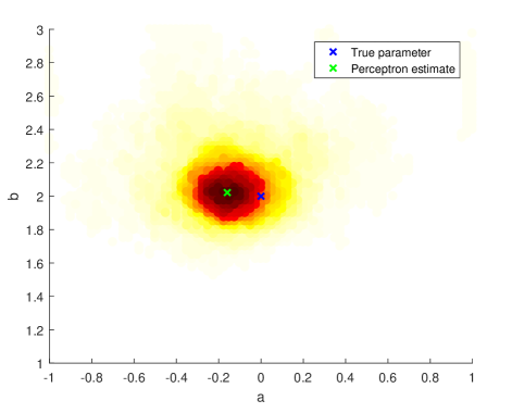
(a) Perceptron-Based Levels

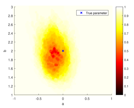
(b) kNN-Based Levels

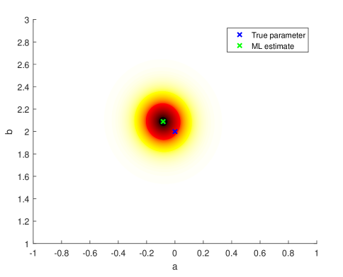
(c) Asymptotic Ellipsoids

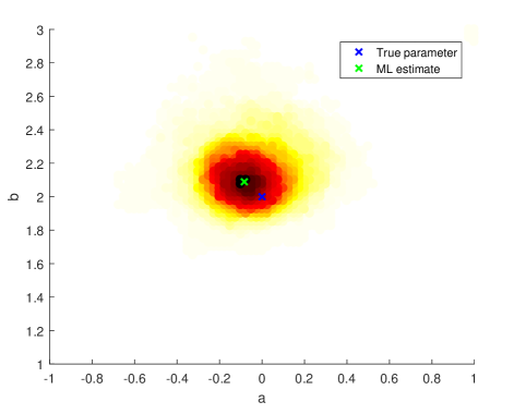
(d) ML-Based Levels

Figure 1: Families of confidence regions for the perceptron-based, the kNN-based and the ML-based resampling scheme are presented along with the asymptotic confidence ellipsoids based on an i.i.d. sample with $n=500$ observations. The distribution of the output variables were discrete uniform and the conditional distribution of an input given the output was Gaussian with different mean values, $\mu_{-1}=-1$ and $\mu_{+1}=1$. We tested a class of logistic functions parameterized by $a$ and $b$, see (68). The true model parameter was $[a_{*},b_{*}]=[0,2]$. The relative ranks are indicated with the colors for each parameter pair on a fine grid. The color bar presents the inclusion probabilities. In the resampling framework altogether we used $m=40$ samples to test each parameter and we applied $k_{n}=\lfloor\sqrt{n}\rfloor$ for the kNN-based algorithm.

In order to emphasize the exactness of our methods, we estimated the coverage probability of the regions with theoretical value $95\%$ based on $30\,000$ Monte Carlo experiments, which is by Hoeffding’s inequality sufficient to reach a $1\%$ precision with probability $99\%$. We tested if the true parameter was included in the confidence region with hyperparameters $m=20$ and $q=1$, and estimated the confidence level by the frequency of the inclusions.

The perceptron-based, the kNN-based and the ML-based construction schemes were all applied. Similarly, we tested if the true parameter was included in the asymptotic confidence ellipsoid with desired level $95\%$ and calculated the frequency of the inclusions. We carried out tests for $n=20$, $50$ and $100$ observations. We can see in Table III that the confidence level of the asymptotic region is conservative and higher than $96\%$ for $n=20$ and $n=50$ instead of the desired $95\%$, while our exact methods are close to the theoretical value for all sample sizes.

We conclude that our non-asymptotic exact guarantee is preferable to the asymptotic one, which is conservative for small samples even if the a priori assumptions are correct.

We carried out similar experiments with a different setup, where the regression function remained the same, but the marginal distribution of the data was changed to a uniform distribution on $[-1,1]$. The results of these trials can be seen in Table IV. Observe that our resampling framework provides exact guarantees for any sample size as before, on the other hand, we can see that the coverage levels of the asymptotic confidence ellipsoids are inaccurate for small sample sizes, though they tend to the theoretic value ($95\%$) as the sample size $n$ increases.

Sample Size	Perceptron	kNN	ML	Ellipsoid
20	95.19 $\%$	95.21 $\%$	95.10 $\%$	96.50 $\%$
50	94.90 $\%$	94.84 $\%$	95.07 $\%$	96.22 $\%$
100	94.83 $\%$	95.01 $\%$	94.88 $\%$	95.86 $\%$

TABLE III: Empirical coverage probabilities (estimated confidence levels) for $n=20$, $50$ and $100$ observations based on $30\,000$ Monte Carlo trials for the perceptron-based, the kNN-based and the ML-based resampling construction and the asymptotic confidence ellipsoids. The underlying conditional marginal distribution of $X$ given $Y$ was normal with mean $Y$ and variance $1$.

Sample Size	Perceptron	kNN	ML	Ellipsoid
20	95,09 $\%$	94.92 $\%$	95.01 $\%$	97.49 $\%$
50	94.69 $\%$	94.99 $\%$	94.90 $\%$	96.63 $\%$
100	94.94 $\%$	94.72 $\%$	94.89 $\%$	95.63 $\%$

TABLE IV: Empirical coverage probabilities (estimated confidence levels) for $n=20$, $50$ and $100$ observations based on $30\,000$ Monte Carlo trials for the perceptron-based, the kNN-based and the ML-based resampling construction and the asymptotic confidence ellipsoids. The underlying marginal distribution was uniform on $[-1,1]$, using the same true regression function as in Table III.

VII Conlusions

In this paper our main goal was to assess the uncertainty of regression models in case of binary classification. The regression function is the key object to deal with in this area, because it is not only sufficient to derive an optimal classifier, but can also be used to determine the probability of misclassification (zero-one risk) at any given input point. The uncertainty regarding the estimated model is quantified in the form of confidence regions.

The paper presented a very flexible resampling framework, which provides exact stochastic guarantees for finding the true underlying regression function. The idea is to test any given candidate by generating alternative samples and comparing those to the original dataset. The strengths of the proposed framework are summarized below:

• The scheme provides finite-sample guarantees for the coverage probability of the true regression function.

• The attained stochastic bounds are distribution-free. We only used that the sample is i.i.d. and the true regression function is included in the given model class $\mathcal{F}_{0}$. Therefore, the distribution of the inputs can be arbitrary and if $\mathcal{F}_{0}$ contains every possible regression function, then the joint distribution of the sample is also unrestricted.

• Any (rational) confidence level can be reached.

• The parameterization of the models can be almost arbitrary, only $\mathcal{L}_{2}(P_{\scriptscriptstyle X})$-injectivity is required, see $A2$.

• The ranking function can be adopted to the problem to build a priori knowledge into the algorithms.

• The framework can be applied for hypothesis testing, in which case the probability of the type I error is explicitly determined for any finite sample.

These can make our framework a promising choice for many real-world uncertainty quantification problems.

We noted earlier that the generality of our framework also allows degenerate constructions. In order to avoid them, we investigated the asymptotic properties of the constructed regions, namely strong pointwise consistency and strong uniform consistency were studied, which hold if the wrong parameters are excluded pointwise or uniformly, respectively. From a hypothesis testing viewpoint, these properties ensure that for any “bad” parameter the probability of type II error tends to zero.

We suggested several specific algorithms with good asymptotic properties, as well. All of them were based on regression function estimation. The idea was to test a given parameter $\theta$, by estimating the regression function from the available datasets. Since the alternative samples are generated with the help of $\theta$, the corresponding estimates should tend to regression function candidate $f_{\theta}$, while the original sample-based estimate should converge to $f_{*}$. Our intention was to statistically detect this difference. We analyzed two main approaches, however, we emphasize that our scheme can be combined with any point estimator.

The first method is based on empirical risk minimization and VC theory. We used least-squares (LS) estimates in the algorithm and proved that if the model class has finite pseudo-dimension and the parameterization is inverse-Lipschitz, then the constructed regions are strongly uniformly consistent, i.e., the confidence sets uniformly shrink around the true parameter. We also proved an exponential PAC-bound, to quantify the probability of inclusion in a given ball around the true parameter. For illustration, several well-known LS-based estimators were revisited.

The condition regarding the model class was weakened for the second method. In fact we allowed $\mathcal{F}_{0}$ to contain all possible regression functions by using nonparametric local averaging estimates, such as kNN or Nadaraya-Watson kernel estimates. Strong pointwise consistency was proved for this variant of our framework, which means that any “bad” parameter is eventually excluded from the confidence regions as the sample size tends to infinity. We quantified the probability of exclusion for a fixed parameter other than $\theta_{*}$ with an exponential bound. One of the main strengths of this latter approach is that no prior knowledge is assumed regarding the model class, hence the second approach is completely distribution-free.

We presented numerical experiments to illustrate our new algorithms. The results showed that our scheme provides comparable regions to the asymptotic ellipsoids. It was demonstrated that the theoretical guarantees are tighter in the resampling framework than in the asymptotic setup, i.e., the confidence level is exact in case of the newly proposed methods, whereas the asymptotic theory usually provides conservative estimates.

A future research direction is to generalize the proposed regression-based construction to more involved nonparametric techniques, such as structural risk minimization, which combine the idea of LS methods with model class complexity theory. Quantifying the size and shape of the regions and giving computationally efficient outer-approximations are also open problems.

Appendix A Proof of Lemma 1

Lemma 1.

Let $A_{1},\dots,A_{m}$ be exchangeable, almost surely pairwise different random elements taking values in $\mathbb{A}$ and let $\psi$ be a ranking function. Then, $\psi\big{(}\,A_{1},A_{2},\dots,A_{m}\,\big{)}$ has discrete uniform distribution, that is for all $k\in[\,m\,]:$

$$\mathbb{P}\big{(}\,\psi\big{(}\,A_{1},A_{2},\dots,A_{m}\,\big{)}=k\,\big{)}=\frac{1}{m}.$$ (70)

Proof.

Random elements $\{A_{i}\}_{i=1}^{m}$ are exchangeable, thus

$$\mathbb{P}\big{(}\,\psi\big{(}\,A_{1},\dots,A_{m}\,\big{)}\,=\,k\,\big{)}$$ (71)

$$=\;\mathbb{P}\big{(}\,\psi\big{(}\,A_{\mu(1)},\dots,A_{\mu(m)}\,\big{)}\,=\,k\,\big{)}$$

for all $k\in[\,m\,]$ and permutation $\mu$ on set $[\,m\,]$. Let us fix the value of $k$. Observe that because of $P1$ we have

$$\big{\{}\,\psi\big{(}\,A_{1},\dots,A_{m}\big{)}=k\,\big{\}}$$ (72)

$$=\big{\{}\,\psi\big{(}\,A_{1},A_{\sigma(2)}\dots,A_{\sigma(m)}\big{)}=k\,\big{\}}$$

for all permutation $\sigma$ on set $\{2,\dots,m\}$. Using the same notation as in $P2$  let $C_{i}\doteq\big{\{}\psi\big{(}\,A_{i},\{A_{j}\}_{j\neq i},\big{)}=k\,\big{\}}$. Notice that events $\big{\{}C_{i}\big{\}}_{i=1}^{m}$ are disjoint because of $P2$. We show that they cover a probability one event. Let $\Omega_{0}$ be the zero probability event which covers those cases when there exists $(i,j)\in[m]\times[m]$ such that $A_{i}=A_{j}$. Because of $P2$ for all $\omega\in\Omega\setminus\Omega_{0}$ values $\psi(A_{j}(\omega),\{A_{k}(\omega)\}_{k\neq j})$ are different for all index $j\in[m]$. By definition these values are included in $[m]$, hence there exists $i\in[m]$ such that $\psi(A_{i}(\omega),\{A_{k}(\omega)\}_{k\neq i})=k$ implying that $\omega\in\textstyle\bigcup_{i=1}^{m}C_{i}$ and $\Omega\setminus\Omega_{0}\subseteq\textstyle\bigcup_{i=1}^{m}C_{i}$. Consequently $\mathbb{P}\Big{(}\textstyle\bigcup_{i=1}^{m}C_{i}\Big{)}=1$. Putting this together with the disjoint property of events $\{C_{i}\}_{i=1}^{m}$, and the exchangeability of $\{A_{i}\}_{i=1}^{m}$ yields

$$1 =\mathbb{P}\big{(}\Omega\setminus\Omega_{0}\big{)}=\mathbb{P}\big{(}\textstyle\bigcup_{i=1}^{m}C_{i}\big{)}=\sum_{i=1}^{m}\mathbb{P}\big{(}C_{i}\big{)}$$ (73)

$$=\sum_{i=1}^{m}\mathbb{P}\big{(}\,\psi\big{(}\,A_{i},\{A_{j}\}_{j\neq i},\big{)}=k\,\big{)}$$

$$=\sum_{i=1}^{m}\mathbb{P}(\psi\big{(}\,A_{1},\{A_{j}\}_{j\neq 1},\big{)}=k\,)$$

$$=m\,\mathbb{P}\big{(}\,\psi\big{(}\,A_{1},\dots,A_{m}\big{)}=k\,\big{)},$$

from which it follows that $\mathbb{P}(\,\psi\big{(}\,A_{1},\dots,A_{m}\big{)}=k\,)=\nicefrac{{1}}{{m}}$ for all $k\in[\,m\,]$. ∎

Appendix B Proofs of Theorem 2 and Theorem 3

Theorem 2.

Assume $A0$, $A1$, $A2$, $B1$ and $B2$, then

$$\mathbb{P}\big{(}\,\theta_{*}\in\Theta_{\varrho,n}^{(1)}\,\big{)}\,=\,\frac{q}{m},$$ (74)

for all sample size $n$. In addition, if $q<m$, then $(\Theta_{\varrho,n}^{(1)})_{n\in\mathbb{N}}$ is strongly uniformly consistent.

The first part of the theorem is already proved in Section IV-A, where the statement about the strong uniform consistency of the constructed regions is deduced from Lemma 2, Lemma 3 and Lemma 4. We present the proof of these here.

Lemma 2.

Let $X_{1},\dots,X_{n}$ be random vectors in $\mathbb{R}^{d}$. If $B2$ holds, then for all $\varepsilon>0$ there exists a real constant $C$ independent of $X_{1},\dots X_{n}$ such that

$$\mathcal{N}_{1}(\,\varepsilon,\mathcal{G},\{X_{1},\dots,X_{n}\}\,)\leq C.$$ (75)

Proof.

First, we show that for any $x_{1},\dots,x_{n}\in\mathbb{X}$ we have

$$\mathcal{N}_{1}(\,\varepsilon,\mathcal{G},\{x_{1},\dots,x_{n}\}\,)$$ (76)

$$\leq\big{(}\mathcal{N}_{1}(\varepsilon/8,\mathcal{F}_{0},\{x_{1},\dots,x_{n}\})\big{)}^{2}.$$

Let $\{f_{1},\dots,f_{k}\}$ be an $\nicefrac{{\varepsilon}}{{8}}$-cover of $\mathcal{F}_{0}$ w.r.t. the $\mathcal{L}_{1}(\mathbb{P}_{n})$ norm with minimal size. It can be assumed w.l.o.g. that $f_{i}$ is bounded between $[-1,1]$ for all $i\in[k]$, otherwise the truncated versions can be used. We argue that $\{\,(f_{i}-f_{j})^{2}\,|\,i,j\in[k]\,\}$ is an $\varepsilon$-cover of $\mathcal{G}$ including at most $k^{2}$ elements. For an arbitrary $h\in\mathcal{G}$ there exist $f,g\in\mathcal{F}_{0}$ such that $h=(f-g)^{2}$. For these functions one can find indexes $i(f),j(g)\in[k]$ such that

$$\left\lVert f-f_{i}\right\rVert_{\mathcal{L}_{1}(\mathbb{P}_{n})}\leq\nicefrac{{\varepsilon}}{{8}},$$ (77)

$$\left\lVert g-f_{j}\right\rVert_{\mathcal{L}_{1}(\mathbb{P}_{n})}\leq\nicefrac{{\varepsilon}}{{8}}.$$

Since $f,g,f_{i}$ and $f_{j}$ are all bounded in $[-1,1]$ and (77) holds, we obtain that

$$\int\big{|}h-(f_{i}-f_{j})^{2}\big{|}\textrm{d}\mathbb{P}_{n}$$ (78)

$$=\int\big{|}(f-g)^{2}-(f_{i}-f_{j})^{2}\big{|}\textrm{d}\mathbb{P}_{n}$$

$$\leq\int\,\big{|}(f-g+f_{i}-f_{j})(f-g-f_{i}+f_{j})\,\big{|}\,\textrm{d}\mathbb{P}_{n}$$

$$\leq 4\int\,\big{|}f-f_{i}\big{|}\,\textrm{d}\mathbb{P}_{n}+4\int\,\big{|}g-f_{j}\big{|}\,\textrm{d}\mathbb{P}_{n}\leq\varepsilon,$$

thus (76) is proved. In the second step we consider function class $\widetilde{\mathcal{F}}\doteq\{\,\nicefrac{{1}}{{2}}(f+1)\,|\,f\in\mathcal{F}_{0}\,\}$ to satisfy the condition of Theorem 7, requiring the boundedness of function each $\tilde{f}\in\widetilde{\mathcal{F}}$ in $[0,1]$. Notice that this transformation does not affect the pseudo-dimension, that is $V_{\mathcal{F}_{0}^{+}}=V_{\widetilde{\mathcal{F}}^{+}}$, and for the covering numbers it holds that

$$\mathcal{N}_{1}(\varepsilon/8,{\mathcal{F}_{0}},\{x_{1},\dots,x_{n}\})$$ (79)

$$\leq\mathcal{N}_{1}(\varepsilon/16,\widetilde{\mathcal{F}},\{x_{1},\dots,x_{n}\}),$$

becuase $\{f_{1},\dots,f_{k}\}$ is an $\varepsilon$-cover of $\mathcal{F}_{0}$ if and only if $\{\nicefrac{{1}}{{2}}(f_{1}+1),\dots,\nicefrac{{1}}{{2}}(f_{k}+1)\}$ is an $\nicefrac{{\varepsilon}}{{2}}$-cover of $\widetilde{\mathcal{F}}$. In the third step we bound the covering numbers with packing numbers by Lemma 6, see [5], as

$$\mathcal{N}_{1}(\varepsilon/16,\widetilde{\mathcal{F}},\{x_{1},\dots,x_{n}\})$$ (80)

$$\leq\mathcal{M}_{1}(\varepsilon/16,\widetilde{\mathcal{F}},\{x_{1},\dots,x_{n}\}).$$

Finally, by Theorem 7 we derive a constant upper bound depending only on pseudo-dimension $V_{\mathcal{F}_{0}^{+}}$ (see [54])

$$\mathcal{M}_{1}(\varepsilon/16,\widetilde{\mathcal{F}},\{x_{1},\dots,x_{n}\})\leq e(V_{\mathcal{F}_{0}^{+}}+1)\bigg{(}\frac{32e}{\varepsilon}\bigg{)}^{\!\!V_{\mathcal{F}_{0}^{+}}},\hskip 2.84526pt$$ (81)

where we used that $V_{\mathcal{F}_{0}^{+}}=V_{\widetilde{\mathcal{F}}^{+}}$. Combining these inequalities yields that $C\doteq e^{2}(V_{\mathcal{F}_{0}^{+}}+1)^{2}\big{(}\frac{32e}{\varepsilon}\big{)}^{2V_{\mathcal{F}_{0}^{+}}}$ is a sought bound on the covering number. ∎

Lemma 3.

Consider the constructed confidence regions in the model space, that is let

$$\mathcal{F}_{\varrho,n}^{(1)}\doteq\big{\{}\,f_{\theta}\in\mathcal{F}_{0}\;|\;\theta\in\Theta_{\varrho,n}^{(1)}\,\big{\}}.$$ (82)

Assume $A0$, $A1$, $A3$ and $B2$, then for all $\varepsilon>0$:

$$\mathbb{P}\,\bigg{(}\,\bigcup_{k=1}^{\infty}\bigcap_{n=k}^{\infty}\left\{\,\mathcal{F}_{\varrho,n}^{(1)}\subseteq B(f_{*},\varepsilon)\,\right\}\bigg{)}\,=\,1,\vspace{0mm}$$ (83)

where $B(f_{*},\varepsilon)\doteq\{f\in\mathcal{F}_{0}\;|\;\left\lVert f-f_{*}\right\rVert_{P}<\varepsilon\}$.

Proof.

We are going to show that $Z_{n}^{(0)}(\theta)$ tends to be the greatest in the ordering, defined by $<_{\pi}$, uniformly for all $\theta\notin B(f_{*},\varepsilon)$ as $n\to\infty$. For $j\in[m-1]$ the difference between the reference variables can be bounded from below as follows

$$Z_{n}^{(0)}(\theta)-Z_{n}^{(j)}(\theta)$$

$$=\frac{1}{n}\sum_{i=1}^{n}(f_{\theta}(X_{i})-f_{\theta,n}^{(0)}(X_{i}))^{2}-\frac{1}{n}\sum_{i=1}^{n}(f_{\theta}(X_{i})-f_{\theta,n}^{(j)}(X_{i}))^{2}$$

$$=\frac{1}{n}\sum_{i=1}^{n}(f_{\theta}(X_{i})-f_{*}(X_{i}))^{2}+\frac{1}{n}\sum_{i=1}^{n}(f_{*}(X_{i})-f_{*,n}^{(0)}(X_{i}))^{2}$$

$$+\frac{2}{n}\sum_{i=1}^{n}(f_{\theta}(X_{i})-f_{*}(X_{i}))(f_{*}(X_{i})-f_{*,n}^{(0)}(X_{i}))$$

$$-\frac{1}{n}\sum_{i=1}^{n}(f_{\theta}(X_{i})-f_{\theta,n}^{(j)}(X_{i}))^{2}\geq\mathbb{E}\big{[}(f_{\theta}(X)-f_{*}(X))^{2}\big{]}$$

$$-\mathbb{E}\big{[}(f_{\theta}(X)-f_{*}(X))^{2}\big{]}+\frac{1}{n}\sum_{i=1}^{n}(f_{\theta}(X_{i})-f_{*}(X_{i}))^{2}$$

$$+\mathbb{E}\big{[}(f_{*}(X)-f_{*,n}^{(0)}(X))^{2}\big{]}-\mathbb{E}\big{[}(f_{*}(X)-f_{*,n}^{(0)}(X))^{2}\big{]}$$

$$+\frac{1}{n}\sum_{i=1}^{n}(f_{*}(X_{i})-f_{*,n}^{(0)}(X_{i}))^{2}-\mathbb{E}\big{[}(f_{\theta}(X)-f_{\theta,n}^{(j)}(X))^{2}\big{]}$$

$$+\mathbb{E}\big{[}(f_{\theta}(X)-f_{\theta,n}^{(j)}(X))^{2}\big{]}-\frac{1}{n}\sum_{i=1}^{n}(f_{\theta}(X_{i})-f_{\theta,n}^{(j)}(X_{i}))^{2}$$

$$-\frac{4}{n}\sum_{i=1}^{n}\big{|}\,f_{*}(X_{i})-f_{*,n}^{(0)}(X_{i})\,\big{|},$$ (84)

where $X$ is independent of $\mathcal{D}_{0}^{\pi}$ and $\mathcal{D}_{j}^{\pi}(\theta)$ and the expectation is with respect to variables $X,\mathcal{D}_{0}$ and $\mathcal{D}_{j}^{\pi}(\theta)$. We want to take the infimum on the left hand side for $f_{\theta}\in\mathcal{F}_{0}\setminus B(f_{*},\varepsilon)$. First, notice that

$$\inf_{f_{\theta}\notin B(f_{*},\varepsilon)}\mathbb{E}\big{[}(f_{\theta}(X)-f_{*}(X))^{2}\big{]}\geq\varepsilon^{2}.$$ (85)

Further, we bound the expectations of the $\mathcal{L}_{2}$-errors:

$$\mathbb{E}\big{[}(f_{*}(X)-f_{*,n}^{(0)}(X))^{2}\big{]}\geq 0,$$ (86)

$$\mathbb{E}\big{[}(f_{\theta}(X)-f_{\theta,n}^{(j)}(X))^{2}\big{]}$$

$$\leq\frac{c_{1}+(c_{2}+c_{3}\log(n))V_{\mathcal{F}_{0}^{+}}}{n}\doteq a_{n},$$

where we used Theorem 8 from Appendix E [5, Theorem 11.5] with the observation that

$$\inf_{f\in\mathcal{F}_{n}}\int\,|\,f(x)-f_{*}(x)\,|^{2}\,\textrm{d}{P_{\scriptscriptstyle X}}(x)=0$$ (87)

follows from $f_{*}\in\mathcal{F}_{n}\doteq\mathcal{F}_{0}$ for all $n\in\mathbb{N}$. Besides, note that $|Y|\leq 1$ and $\sup_{x\in\mathbb{R}^{d}}|f(x)|\leq 1$ for all $f\in\mathcal{F}_{0}$, therefore Theorem 8 can be applied directly and the truncation does not affect the estimators.

The deviations from the expected values are bounded with a supremum over $\mathcal{F}_{0}$ as

$$\mathbb{E}\big{[}(f_{\theta}(X)-f_{*}(X))^{2}\big{]}-\frac{1}{n}\sum_{i=1}^{n}(f_{\theta}(X_{i})-f_{*}(X_{i}))^{2}$$

$$+\mathbb{E}\big{[}(f_{*}(X)-f_{*,n}^{(0)}(X))^{2}\big{]}-\frac{1}{n}\sum_{i=1}^{n}(f_{*}(X_{i})-f_{*,n}^{(0)}(X_{i}))^{2}$$

$$-\mathbb{E}\big{[}(f_{\theta}(X)-f_{\theta,n}^{(j)}(X))^{2}\big{]}+\frac{1}{n}\sum_{i=1}^{n}(f_{\theta}(X_{i})-f_{\theta,n}^{(j)}(X_{i}))^{2}\leq$$

$$3\sup_{f,g\in\mathcal{F}_{0}}\Big{|}\,\frac{1}{n}\sum_{i=1}^{n}(f(X_{i})-g(X_{i}))^{2}-\mathbb{E}\big{[}(f(X)-g(X))^{2}\big{]}\Big{|}$$

$$=3\sup_{h\in\mathcal{G}}\Big{|}\,\frac{1}{n}\sum_{i=1}^{n}h(X_{i})-\mathbb{E}h(X)\Big{|},$$ (88)

where $\mathcal{G}$ is defined in (25). The inequality holds because $f_{\theta}$, $f_{*}$ and the estimators are all included in $\mathcal{F}_{0}$.

For the quarter of the last term in (84) we apply the Cauchy–Schwartz inequality, then we bound the obtained value with the same supremum as in (88) plus the zero sequence $a_{n}$, defined in (86), as

$$\Big{(}\frac{1}{n}\sum_{i=1}^{n}\big{|}\,f_{*}(X_{i})-f_{*,n}^{(0)}(X_{i})\,\big{|}\Big{)}^{2}$$

$$\leq\frac{1}{n^{2}}\sum_{i=1}^{n}(f_{*}(X_{i})-f_{*,n}^{(0)}(X_{i}))^{2}\sum_{i=1}^{n}1$$

$$\leq\frac{1}{n}\sum_{i=1}^{n}(f_{*}(X_{i})-f_{*,n}^{(0)}(X_{i}))^{2}$$

$$-\mathbb{E}\big{[}(f_{*}(X)-f_{*,n}^{(0)}(X))^{2}\big{]}+\mathbb{E}\big{[}(f_{*}(X)-f_{*,n}^{(0)}(X))^{2}\big{]}$$

$$\leq\sup_{f,g\in\mathcal{F}_{0}}\Big{|}\,\frac{1}{n}\sum_{i=1}^{n}(f(X_{i})-g(X_{i}))^{2}-\mathbb{E}\big{[}(f(X)-g(X))^{2}\big{]}\,\Big{|}$$

$$+a_{n}=\sup_{h\in\mathcal{G}}\Big{|}\,\frac{1}{n}\sum_{i=1}^{n}h(X_{i})-\mathbb{E}h(X)\Big{|}+a_{n}.$$ (89)

For the sake of simplicity let

$$A_{n}\doteq\sup_{h\in\mathcal{G}}\Big{|}\,\frac{1}{n}\sum_{i=1}^{n}h(X_{i})-\mathbb{E}h(X)\,\Big{|}.$$ (90)

To sum up, we can bound the infimum of the difference between two reference variables from below as

$$\begin{gathered}\inf_{f_{\theta}\notin B(f_{*},\varepsilon)}(Z_{n}^{(0)}(\theta)-Z_{n}^{(j)}(\theta))\geq\varepsilon^{2}-a_{n}\\ -3A_{n}-4\sqrt{A_{n}+a_{n}}.\end{gathered}$$ (91)

Observe that $a_{n}$ is deterministic and tends to zero as $n\to\infty$. If $A_{n}$ converges to zero almost surely, then for all $j\in[m-1]$ a.s. there exists $n_{j}\in\mathbb{N}$ such that for all $n>n_{j}$ the $Z_{n}^{(0)}(\theta)-Z_{n}^{(j)}(\theta)$ difference becomes positive for all $f_{\theta}\notin B(f_{*},\varepsilon)$, and by the construction for all $n>\max_{j\in[m-1]}n_{j}$ we have $\mathcal{F}_{\varrho,n}^{(1)}\subseteq B(f_{*},\varepsilon)$.

It remained to prove that $A_{n}\xrightarrow{\,a.s.\,}0$. We need to use a uniform law of large numbers. By Lemma 2 the assumption of Theorem 9 is satisfied, i.e., for all $\varepsilon>0$ we have

$$\begin{gathered}\sum_{n=1}^{\infty}\mathbb{E}\big{(}\,\mathcal{N}_{1}(\varepsilon/8,\mathcal{G},\{X_{1},\dots,X_{n}\})\,\big{)}e^{-\nicefrac{{n\varepsilon^{2}}}{{(128B^{2})}}}\\ \leq C\cdot\sum_{n=1}^{\infty}e^{-\nicefrac{{n\varepsilon^{2}}}{{(128B^{2})}}}<\infty,\end{gathered}$$ (92)

where $B=4$, because $(f(x)-g(x))^{2}\in[0,4]$ for all $x\in\mathbb{X}$ and $f,g\in\mathcal{F}_{0}$. Consequently $A_{n}\xrightarrow{\,a.s.\,}0$ holds. ∎

Lemma 4.

If (31) holds for all $\varepsilon>0$ and $A2$, $B1$ hold true, then for all $\varepsilon>0$ we have

$$\mathbb{P}\,\bigg{(}\,\bigcup_{k=1}^{\infty}\bigcap_{n=k}^{\infty}\left\{\,\Theta_{\varrho,n}^{(1)}\subseteq B(\theta_{*},\varepsilon)\,\right\}\bigg{)}\,=\,1.\vspace{0mm}$$ (93)

Proof.

If $f_{\theta}\in B(f_{*},\nicefrac{{\varepsilon}}{{L}})$, then $\theta\in B(\theta_{*},\varepsilon)$, because of $B1$. Hence, it follows that

$$\left\{\,\Theta_{\varrho,n}^{(1)}\subseteq B(\theta_{*},\varepsilon)\,\right\}\supseteq\left\{\,\mathcal{F}_{\varrho,n}^{(1)}\subseteq B(f_{*},\nicefrac{{\varepsilon}}{{L}})\,\right\}.$$ (94)

The inclusion also holds for the $\liminf$ of events. Finally, since (31) holds for $\nicefrac{{\varepsilon}}{{L}}$ by (94) we also have (93). ∎

Theorem 3.

Assume $A0$, $A1$, $A2$, $A3$, $B1$, $B2$ and $q<m$, then for all $\varepsilon>0$ for $n$ large enough we have

$$\mathbb{P}\,\big{(}\,\Theta_{\varrho,n}^{(1)}\subseteq B(\theta_{*},\varepsilon)\,\big{)}\geq 1-C_{1}e^{-n\lambda_{1}},$$ (95)

where $C$ depends only on $\varepsilon$ and $V_{\mathcal{F}_{0}^{+}}$, and $\lambda_{1}$ depends only on $\varepsilon$ and Lipschitz constant $L$.

Proof of Theorem 3.

Similarly as in the proof of Theorem 2 observe that

$$\begin{gathered}\big{\{}\Theta_{\varrho,n}^{(1)}\subseteq B(\theta_{*},\varepsilon)\big{\}}\supseteq\\ \big{\{}\forall j\in[m-1]:\inf_{\theta\notin B(\theta_{*},\varepsilon)}\big{(}Z_{n}^{(0)}(\theta)-Z_{n}^{(j)}(\theta)\big{)}>0\big{\}}.\end{gathered}$$ (96)

By Lemma 4 and (91) we obtain for all $j\in[m-1]$ that

$$\inf_{\theta\notin B(\theta_{*},\varepsilon)}\big{(}Z_{n}^{(0)}(\theta)-Z_{n}^{(j)}(\theta)\big{)}$$ (97)

$$\geq\inf_{f_{\theta}\notin B(f_{*},\varepsilon/L)}\big{(}Z_{n}^{(0)}(\theta)-Z_{n}^{(j)}(\theta)\big{)}$$

$$\geq\frac{\varepsilon^{2}}{L^{2}}-a_{n}-3A_{n}-4\sqrt{A_{n}+a_{n}},$$

where $L$ is the Lipschitz constant, $a_{n}$ is a deterministic zero sequence defined in (86) and $A_{n}$ is the random (measurable) supremum of the deviations defined in (90). Notice that the lower bound does not depend on index $j$, consequently by elementary manipulations we gain

$$\;\mathbb{P}\big{(}\,\Theta_{\varrho,n}^{(1)}\subseteq B(\theta_{*},\varepsilon)\,\big{)}$$ (98)

$$\geq\mathbb{P}\big{(}\forall j\in[m-1]:\inf_{\theta\notin B(\theta_{*},\varepsilon)}\big{(}Z_{n}^{(0)}(\theta)-Z_{n}^{(j)}(\theta)\big{)}>0\big{)}$$

$$\geq\mathbb{P}\big{(}\forall j\in[m-1]:\inf_{f_{\theta}\notin B(f_{*},\varepsilon/L)}\big{(}Z_{n}^{(0)}(\theta)-Z_{n}^{(j)}(\theta)\big{)}>0\big{)}$$

$$\geq\mathbb{P}\bigg{(}\,\frac{\varepsilon^{2}}{2L^{2}}>a_{n}+3A_{n}+4\sqrt{A_{n}+a_{n}}\,\bigg{)}$$

$$\geq\mathbb{P}\bigg{(}\,\frac{\varepsilon^{2}}{6L^{2}}>a_{n},\frac{\varepsilon^{2}}{6L^{2}}\geq 3A_{n},\frac{\varepsilon^{2}}{6L^{2}}\geq 4\sqrt{A_{n}+a_{n}}\,\bigg{)}$$

$$=\mathbb{P}\bigg{(}\,\frac{\varepsilon^{2}}{6L^{2}}>a_{n},\frac{\varepsilon^{2}}{18L^{2}}\geq A_{n},\frac{\varepsilon^{4}}{24^{2}L^{4}}\geq A_{n}+a_{n}\,\bigg{)}$$

$$\geq\mathbb{P}\bigg{(}\min\Big{(}\frac{\varepsilon^{2}}{6L^{2}},\frac{\varepsilon^{4}}{2\cdot 24^{2}L^{4}}\Big{)}>a_{n},$$

$$\;\;\;\;\hskip 71.13188pt\min\Big{(}\frac{\varepsilon^{2}}{18L^{2}},\frac{\varepsilon^{4}}{2\cdot 24^{2}L^{4}}\Big{)}\geq A_{n}\bigg{)}.$$

Since $a_{n}$ is deterministic and tends to zero we can find $n_{0}$ such that for all $n>n_{0}$:

$$\gamma\doteq\min\Big{(}\frac{\varepsilon^{2}}{6L^{2}},\frac{\varepsilon^{4}}{2\cdot 24^{2}L^{4}}\Big{)}>a_{n}$$ (99)

holds. Furthermore let

$$\tau\doteq\min\Big{(}\frac{\varepsilon^{2}}{18L^{2}},\frac{\varepsilon^{4}}{2\cdot 24^{2}L^{4}}\Big{)}$$ (100)

Then by Theorem 9 and Lemma 2 for $n>n_{0}$ we have

$$\mathbb{P}(A_{n}\leq\tau)=1-\mathbb{P}(A_{n}>\tau)$$ (101)

$$\geq 1-8\cdot C\cdot\exp\Big{(}-\frac{n\tau^{2}}{128B^{2}}\Big{)},$$

where $B=4$. Consequently with constants $C_{1}\doteq 8C$ and $\lambda_{1}\doteq\frac{\tau^{2}}{128B^{2}}$ Theorem 3 follows. ∎

Lemma 5.

Let $\mathcal{F}_{0}$ be a finite dimensional linear subspace of $\mathcal{L}_{2}(P_{\scriptscriptstyle X})$ spanned by an orthonormal system of vectors $\{\varphi_{1},\dots,\varphi_{k}\}$. Then the linear parameterization is an isometry, i.e., for all $\alpha,\beta\in\mathbb{R}^{k}$ we have

$$\left\lVert\alpha-\beta\right\rVert_{2}=\Big{\|}\sum_{i=1}^{k}\alpha_{i}\varphi_{i}(x)-\sum_{i=1}^{k}\beta_{i}\varphi_{i}(x)\Big{\|}_{\scriptscriptstyle P},$$ (102)

henceforth it is also inverse Lipschitz-continuous.

Proof.

The orthonormality of $\varphi_{1},\dots,\varphi_{k}$ implies (102). ∎

Appendix C Proof of Theorem 4 and Theorem 5

Theorem 4.

Assume $A0$, $A1$, $A2$ and $A3$, then

$$\mathbb{P}\big{(}\,\theta_{*}\in\Theta_{\varrho,n}^{(2)}\,\big{)}\,=\,\frac{q}{m},$$ (103)

for all sample size $n$. Furthermore, if $q<m$, $\nicefrac{{k_{n}}}{{n}}\to 0$, and there is $\delta>0$ such that $\nicefrac{{k_{n}^{2}}}{{n^{(1+\delta)}}}\to\infty$ as $n\to\infty$, then $(\,\Theta_{\varrho,n}^{(2)}\,)_{n\in\mathbb{N}}$ is strongly pointwise consistent for all distribution of $(X,Y)$ which satisfy

$$\mathbb{P}\big{(}\,\left\lVert X-X^{\prime}\right\rVert_{2}\neq\left\lVert X-X^{\prime\prime}\right\rVert_{2}\,\big{)}=1,$$ (104)

where $X^{\prime}$ and $X^{\prime\prime}$ are independent copies of $X$.

Proof of Theorem 4.

We are going to show that for $\theta\neq\theta_{*}$ reference variable $Z_{n}^{(0)}(\theta)$ tends to be the greatest in the ordering. The proof will be presented in two steps. First we reduce the problem to the almost sure convergence of empirical $\mathcal{L}_{1}$-errors to zero, then we prove that the convergence holds for the kNN estimates.

Let $\theta\neq\theta_{*}$ and fix an index $j\in[m-1]$. We bound the difference between the reference variables from below as

$$Z_{n}^{(0)}(\theta)-Z_{n}^{(j)}(\theta)=$$

$$\frac{1}{n}\sum_{i=1}^{n}\big{(}f_{\theta}(X_{i})-f_{*,n}^{(0)}(X_{i})\big{)}^{2}-\frac{1}{n}\sum_{i=1}^{n}\big{(}f_{\theta}(X_{i})-f_{\theta,n}^{(j)}(X_{i})\big{)}^{2}$$

$$=\frac{1}{n}\sum_{i=1}^{n}\big{(}f_{\theta}(X_{i})-f_{*}(X_{i})\big{)}^{2}\!+\frac{1}{n}\sum_{i=1}^{n}\big{(}f_{*}(X_{i})-f_{*,n}^{(0)}(X_{i})\big{)}^{2}$$ (105)

$$+\frac{2}{n}\sum_{i=1}^{n}\big{(}f_{\theta}(X_{i})-f_{*}(X_{i})\big{)}\big{(}f_{*}(X_{i})-f_{*,n}^{(0)}(X_{i})\big{)}$$

$$-\frac{1}{n}\sum_{i=1}^{n}\big{(}f_{\theta}(X_{i})-f_{\theta,n}^{(j)}(X_{i})\big{)}^{2}$$

$$\geq\frac{1}{n}\sum_{i=1}^{n}\big{(}\,f_{\theta}(X_{i})-f_{*}(X_{i})\,\big{)}^{2}-\frac{2}{n}\sum_{i=1}^{n}\big{|}\,f_{*}(X_{i})-f_{*,n}^{(0)}(X_{i})\,\big{|}$$

$$-\frac{4}{n}\sum_{i=1}^{n}\big{|}\,f_{*}(X_{i})-f_{*,n}^{(0)}(X_{i})\,\big{|}-\frac{2}{n}\sum_{i=1}^{n}\big{|}\,f_{\theta}(X_{i})-f_{\theta,n}^{(j)}(X_{i})\,\big{|},$$

where we used that $f_{\theta}$, $f_{*}$ and the estimators are all bounded in $[-1,1]$. Observe that by the strong law of large numbers as $n\to\infty$ the following holds

$$\frac{1}{n}\sum_{i=1}^{n}\big{(}\,f_{\theta}(X_{i})-f_{*}(X_{i})\,\big{)}^{2}\xrightarrow{\,a.s.\,}\kappa^{2}\doteq\left\lVert f_{\theta}-f_{*}\right\rVert_{P}^{2},$$ (106)

where $\kappa>0$, because of $A2$. It remained to prove that

$$\frac{1}{n}\sum_{i=1}^{n}\big{|}\,f_{*}(X_{i})-f_{*,n}^{(0)}(X_{i})\,\big{|}\xrightarrow{\,a.s.\,}0,$$ (107)

$$\frac{1}{n}\sum_{i=1}^{n}\big{|}\,f_{\theta}(X_{i})-f_{\theta,n}^{(j)}(X_{i})\,\big{|}\xrightarrow{\,a.s.\,}0$$ (108)

hold. As in the proof of Theorem 2, then a.s. there exists $n_{j}$ such that the quantity in (105) becomes positive, therefore for all $n>\max_{j\in[m-1]}n_{j}$ we have $\theta\notin\Theta_{\varrho,n}^{(2)}$.

Notice that it is sufficient for (107) and (108) to prove for any possible regression function $f$ that

$$\frac{1}{n}\sum_{i=1}^{n}\big{|}\,f_{n}(X_{i})-f(X_{i})\,\big{|}\xrightarrow{\,a.s.\,}0$$ (109)

holds, where $f_{n}$ is the kNN estimator of $f$ based on $\{(X_{i},Y_{i})\}_{i=1}^{n}$ with $k_{n}$ neighbors. Hence, we need to prove the consistency of an empirical $\mathcal{L}_{1}$-error for all distributions of $(X,Y)$ such that (104) holds. In order to obtain (109) we use the following decomposition:

$$\frac{1}{n}\sum_{i=1}^{n}\big{|}\,f_{n}(X_{i})-f(X_{i})\,\big{|}=\frac{1}{n}\sum_{i=1}^{n}\big{|}\,f_{n}(X_{i})-f(X_{i})\,\big{|}$$

$$-\mathbb{E}\Big{[}\frac{1}{n}\sum_{i=1}^{n}\big{|}\,f_{n}(X_{i})-f(X_{i})\,\big{|}\Big{]}+\mathbb{E}\Big{[}\frac{1}{n}\sum_{i=1}^{n}\big{|}\,f_{n}(X_{i})-f(X_{i})\,\big{|}\Big{]}$$

$$\leq\Big{|}\frac{1}{n}\sum_{i=1}^{n}\big{|}\,f_{n}(X_{i})-f(X_{i})\,\big{|}-\mathbb{E}\Big{[}\frac{1}{n}\sum_{i=1}^{n}\big{|}\,f_{n}(X_{i})-f(X_{i})\,\big{|}\Big{]}\Big{|}$$

$$+\mathbb{E}\Big{[}\frac{1}{n}\sum_{i=1}^{n}\big{|}\,f_{n}(X_{i})-f(X_{i})\,\big{|}\Big{]}.$$ (110)

First, we prove that the expected value converges to zero, then we apply McDiarmid’s inequality [55] to show that the empirical $\mathcal{L}_{1}$-error is concentrated around its expectation. By the linearity of the expectation and the i.i.d. property of the sample we obtain

$$\mathbb{E}\Big{[}\frac{1}{n}\sum_{i=1}^{n}\big{|}\,f_{n}(X_{i})-f(X_{i})\,\big{|}\Big{]}=\mathbb{E}\big{|}\,f_{n}(X_{n})-f(X_{n})\,\big{|}$$

$$=\mathbb{E}\Big{|}\,\frac{1}{k_{n}}\sum_{i=1}^{n}Y_{i}\mathbb{I}(X_{i}\in N_{n}(X_{n},k_{n}))-f(X_{n})\,\Big{|}$$

$$=\frac{1}{k_{n}}\mathbb{E}\Big{|}\sum_{i=1}^{n}(Y_{i}-f(X_{n}))\mathbb{I}(X_{i}\in N_{n}(X_{n},k_{n}))\,\Big{|}$$

$$\leq\mathbb{E}\Big{|}\frac{1}{k_{n}}\sum_{i=1}^{n-1}(Y_{i}-f(X_{n}))\mathbb{I}(X_{i}\in N_{n}(X_{n},k_{n}))\Big{|}$$

$$+\frac{1}{k_{n}}\mathbb{E}\big{|}Y_{n}-f(X_{n})\big{|}\leq$$

$$\mathbb{E}\Big{|}\frac{1}{k_{n}-1}\!\sum_{i=1}^{n-1}(Y_{i}-f(X_{n}))\mathbb{I}(X_{i}\in N_{n-1}(X_{n},k_{n}\!-1))\Big{|}\!+\!\frac{2}{k_{n}}$$

$$\leq\mathbb{E}\big{|}f_{n-1}^{\prime}(X_{n})-f(X_{n})\big{|}+\frac{2}{k_{n}},$$ (111)

where $f_{n-1}^{\prime}$ is a kNN estimate based on $\{(X_{i},Y_{i})\}_{i=1}^{n-1}$ with $k_{n}-1$ neighbors. Clearly, $\nicefrac{{2}}{{k_{n}}}\to 0$ as $n\to\infty$. In addition, by the weak consistency of the kNN method (Theorem 10)

$$\mathbb{E}\big{|}f_{n-1}^{\prime}(X_{n})-f(X_{n})\big{|}$$ (112)

$$\leq\sqrt{\mathbb{E}\big{[}\,\big{|}f_{n-1}^{\prime}(X_{n})-f(X_{n})\big{|}^{2}\,\big{]}}\to 0,$$

because $(k_{n}-1)\to\infty$ and $\nicefrac{{k_{n}-1}}{{n}}\to 0$ as $n\to\infty$ and $X_{n}$ is independent of $\{(X_{i},Y_{i})\}_{i=1}^{n-1}$.

In the last step we apply McDiarmid’s inequality, see Theorem 11, to bound the difference between the empirical error and the expected value. Let $\mathcal{D}\doteq\{(x_{i},y_{i})\}_{i=1}^{n}$ and $g:(\mathbb{X}\times\mathbb{Y})^{n}\to\mathbb{R}^{+}$ be the following function

$$\begin{gathered}g((x_{1},y_{1}),\dots,(x_{n}.y_{n}))\doteq\frac{1}{n}\sum_{i=1}^{n}\big{|}\,f_{n}^{\mathcal{D}}(x_{i})-f(x_{i})\,\big{|},\end{gathered}$$ (113)

where $f_{n}^{\mathcal{D}}(x)\doteq\nicefrac{{1}}{{k_{n}}}\sum_{i=1}^{n}y_{i}\mathbb{I}(x_{i}\in N(x,k_{n}))$. Observe that $g$ satisfies the bounded difference property (139). If two samples, $\mathcal{D}_{1}$ and $\mathcal{D}_{2}$, differ only in one pair $(x_{i},y_{i})$, then

$$\big{|}f_{n}^{\mathcal{D}_{1}}(x)-f_{n}^{\mathcal{D}_{2}}(x)\big{|}\leq\nicefrac{{2}}{{k_{n}}}$$ (114)

holds for all $x\in\mathbb{X}$. Hence by the reverse triangle inequality

$$|\,g(\mathcal{D}_{1})-g(\mathcal{D}_{2})\,|\leq\frac{2}{k_{n}}.$$ (115)

Consequently, by Theorem 11 we obtain

$$\mathbb{P}\big{(}\,\big{|}g(\mathcal{D})-\mathbb{E}g(\mathcal{D})\big{|}\geq\varepsilon\,\big{)}\leq 2\exp\bigg{(}-\frac{k_{n}^{2}\varepsilon^{2}}{2n}\bigg{)}.$$ (116)

By $\nicefrac{{k_{n}^{2}}}{{n^{1+\delta}}}\to\infty$ for $n$ large enough

$$\exp\bigg{(}-\frac{k_{n}^{2}n^{\delta}\varepsilon^{2}}{2n^{1+\delta}}\bigg{)}\leq\exp\bigg{(}-\frac{n^{\delta}\varepsilon^{2}}{2}\bigg{)},$$ (117)

where the right hand side is summable. Then the application of the Borel–Cantelli lemma yields that

$$\limsup_{n\to\infty}\big{|}g(\mathcal{D})-\mathbb{E}g(\mathcal{D})\big{|}<\varepsilon$$ (118)

almost surely. Because we have (118) for all $\varepsilon>0$,

$$\big{|}g(\mathcal{D})-\mathbb{E}g(\mathcal{D})\big{|}\xrightarrow{\,a.s.\,}0,$$ (119)

hence the convergence in (109) is proved. ∎

Theorem 5.

Assume that $A0$, $A1$, $A2$, $A3$ and $q<m$ hold. In addition, $\nicefrac{{k_{n}}}{{n}}\to 0$, and there exists $\delta>0$ such that $\nicefrac{{k_{n}^{2}}}{{n^{(1+\delta)}}}\to\infty$ as $n\to\infty$. For every distribution of $(X,Y)$ such that  $\mathbb{P}\big{(}\left\lVert X-X^{\prime}\right\rVert_{2}\neq\left\lVert X-X^{\prime\prime}\right\rVert_{2}\big{)}=1,$ where $X^{\prime}$ and $X^{\prime\prime}$ are independent copies of $X$, for a given $\theta\in\Theta$, $\theta\neq\theta_{*}$, there exists $N_{0}$ such that for $n\geq N_{0}$ we have

$$\mathbb{P}\big{(}\,\theta\notin\Theta_{\varrho,n}^{(2)}\,\big{)}\geq 1-C_{2}e^{-\nicefrac{{k_{n}^{2}\lambda_{2}}}{{n}}},$$ (120)

where $C_{2}$ depends only on $m$, the number of datasets, and $\lambda_{2}$ depends on $\|f_{\theta}-f_{*}\|_{\scriptscriptstyle P}$.

Proof.

For the sake of simplicity let

$$I_{n}\doteq\frac{1}{n}\sum_{i=1}^{n}(f_{\theta}(X_{i})-f_{*}(X_{i}))^{2},$$ (121)

$$J_{n}\doteq\frac{6}{n}\sum_{i=1}^{n}\big{|}\,f_{*}(X_{i})-f_{*,n}(X_{i})\,\big{|},$$

$$K_{n}^{(j)}\doteq\frac{2}{n}\sum_{i=1}^{n}\big{|}\,f_{\theta}(X_{i})-f_{\theta,n}^{(j)}(X_{i})\,\big{|}$$

for $j\in[m-1]$. Since $Z_{n}^{(0)}(\theta)-Z_{n}^{(j)}(\theta)$ can be lower bounded by $I_{n}-J_{n}-K_{n}^{(j)}$, see (105), we have

$$\begin{gathered}\{\theta\notin\Theta_{\varrho,n}^{(2)}\}\supseteq\big{\{}\forall j\in[m-1]:I_{n}-J_{n}-K_{n}^{(j)}>0\big{\}}.\end{gathered}$$

Let $\kappa\doteq\|f_{\theta}-f_{*}\|_{\scriptscriptstyle P}^{2}$. Then, by De Morgan’s law and the union bound, we have

$$\mathbb{P}(\theta\notin\Theta_{\varrho,n}^{(2)})\geq\mathbb{P}(\forall j\in[m-1]:I_{n}-J_{n}-K_{n}^{(j)}>0)$$

$$\geq\mathbb{P}(I_{n}\geq\nicefrac{{\kappa}}{{2}},J_{n}<\nicefrac{{\kappa}}{{4}},\forall j\in[m-1]:K_{n}^{(j)}<\nicefrac{{\kappa}}{{4}})$$

$$\geq 1-\mathbb{P}(I_{n}<\nicefrac{{\kappa}}{{2}})-\mathbb{P}(J_{n}\geq\nicefrac{{\kappa}}{{4}})-\sum_{j=1}^{m-1}\mathbb{P}(K_{n}^{(j)}\geq\nicefrac{{\kappa}}{{4}}).$$

We will bound these terms separately. First, let

$$\xi_{i}\doteq(f_{\theta}(X_{i})-f_{*}(X_{i}))^{2}$$ (122)

for all $i\in[n]$. By Hoeffding’s inequality

$$\mathbb{P}(\,I_{n}<\nicefrac{{\kappa}}{{2}}\,)=\mathbb{P}(\,I_{n}-\kappa<-\nicefrac{{\kappa}}{{2}}\,)$$ (123)

$$\leq\mathbb{P}\Big{(}\,\Big{|}\frac{1}{n}\sum_{i=1}^{n}\xi_{i}-\mathbb{E}\xi_{1}\Big{|}>\nicefrac{{\kappa}}{{2}}\,\Big{)}\leq 2e^{-\nicefrac{{2n\kappa^{2}}}{{4^{2}}}}$$

$$\leq 2e^{-\nicefrac{{k_{n}^{2}\kappa^{2}}}{{n8}}}.$$

For the second term notice that

$$\begin{gathered}\{J_{n}\geq\nicefrac{{\kappa}}{{4}}\}\subseteq\\ \big{\{}|J_{n}-\mathbb{E}J_{n}|\geq|\,\nicefrac{{\kappa}}{{4}}-\mathbb{E}J_{n}\,|\big{\}}\Big{)}.\end{gathered}$$ (124)

For $n$ large enough, see (111) and Theorem 10, $\mathbb{E}J_{n}\leq\nicefrac{{\kappa}}{{8}}$ holds. Furthermore, by McDiarmid’s inequality, see the proof of Theorem 4, we have

$$\begin{gathered}\mathbb{P}\,\big{(}\,|J_{n}-\mathbb{E}J_{n}|\geq\nicefrac{{\kappa}}{{8}}\,\big{)}\leq\exp\Big{(}-\frac{k_{n}^{2}\kappa^{2}}{2\cdot 24^{2}n}\Big{)}.\end{gathered}$$ (125)

Combining these yields that for $n$ large enough

$$\begin{gathered}\mathbb{P}\,(\,J_{n}\geq\nicefrac{{\kappa}}{{4}}\,)\leq\mathbb{P}\,\big{(}\,|J_{n}-\mathbb{E}J_{n}|\geq\nicefrac{{\kappa}}{{8}}\,\big{)}\\ \leq 2\exp\Big{(}-\frac{k_{n}^{2}\kappa^{2}}{2\cdot 48^{2}n}\Big{)}\end{gathered}$$ (126)

For the last term observe that $\{K_{n}^{(j)}\}_{j=1}^{m-1}$ are identically distributed, therefore

$$\sum_{j=1}^{m-1}\mathbb{P}\,(\,K_{n}^{(j)}\geq\nicefrac{{\kappa}}{{4}}\,)=(m-1)\,\mathbb{P}\,(\,K_{n}^{(1)}\geq\nicefrac{{\kappa}}{{4}}\,).$$ (127)

In addition, since $K_{n}^{(j)}$ is a similar quantity as $J_{n}$ for a different model parameter, the same argument as above yields the exponential upper bound, see (126), on the probability of $\big{\{}K_{n}^{(j)}\geq\nicefrac{{\kappa}}{{4}}\big{\}}$ for $n$ large enough.

We obtain the claim of the theorem, namely (120), by merging these exponential bounds together as

$$\mathbb{P}\big{(}\,\theta\notin\Theta_{\varrho,n}^{(2)}\,\big{)}\geq 1-(4+2(m-1))\exp\Big{(}-\frac{k_{n}^{2}\lambda_{2}}{n}\Big{)},$$ (128)

for $n$ large enough, where $\lambda_{2}\doteq\frac{\kappa^{2}}{2\cdot 48^{2}}$. ∎

Appendix D Proof of Theorem 6

Theorem 6.

Assume $A0$, $A1$, $A2$, $A3$ and $C1$. Then

$$\mathbb{P}\big{(}\,\theta_{*}\in\Theta_{\varrho,n}^{(3)}\,\big{)}\,=\,\frac{q}{m},$$ (129)

for all sample size $n$. Furthermore, if $q<m$, then $(\,\Theta_{\varrho,n}^{(3)}\,)_{n\in\mathbb{N}}$ is strongly consistent.

Proof.

The claim concerning the exact coverage probability is a corollary of Lemma 1.

For strong pointwise consistency let $\theta\neq\theta_{*}$ and fix an index $j\in[m-1]$. In order to prove the almost sure convergence of the examined parameter we bound the difference of reference variables from below as

$$Z_{n}^{(0)}(\theta)-Z_{n}^{(j)}(\theta)$$

$$\geq\frac{1}{n}\sum_{i=1}^{n}\big{(}f_{\theta}(X_{i})-f_{*}(X_{i})\big{)}^{2}-\frac{2}{n}\sum_{i=1}^{n}\big{|}f_{*}(X_{i})-f_{*,n}^{(0)}(X_{i})\big{|}$$

$$-\frac{4}{n}\sum_{i=1}^{n}\big{|}f_{*}(X_{i})-f_{*,n}^{(0)}(X_{i})\big{|}-\frac{2}{n}\sum_{i=1}^{n}\big{|}f_{\theta}(X_{i})-f_{\theta,n}^{(j)}(X_{i})\big{|},$$

$$\geq\frac{1}{n}\sum_{i=1}^{n}\big{(}\,f_{\theta}(X_{i})-f_{*}(X_{i})\,\big{)}^{2}-6\sup_{x\in\mathbb{X}}\big{|}\,f_{*}(x)-f_{*,n}^{(0)}(x)\,\big{|}$$

$$-2\sup_{x\in\mathbb{X}}\big{|}\,f_{\theta}(x)-f_{\theta,n}^{(j)}(x)\,\big{|},$$ (130)

where the first inequality is justified by (105). The first term converges to $\kappa=\left\lVert f_{\theta}-f_{*}\right\rVert_{P}^{2}$ by the SLLN. The second and third terms converge to zero by the uniform consistency of the regression function estimate ($C1$). From this point on, the proof can be finished very similarly as above, see the proof of Theorem 4. ∎

Appendix E Fundamental Results used in the Proofs

In the proof of Lemma 2 we used Lemma 6 and Theorem 7. The following lemma establishes a close relationship between packing and covering numbers, see [5, Lemma 9.2]

Lemma 6.

Let $\mathcal{F}$ be a class of functions on $\mathbb{R}^{d}$, $P_{\scriptscriptstyle X}$ be a probability measure on $\mathbb{R}^{d}$ and $\left\lVert\cdot\right\rVert\doteq\left\lVert\cdot\right\rVert_{\mathcal{L}_{1}(P_{\scriptscriptstyle X})}$ be the $\mathcal{L}_{1}$ norm on $\mathcal{F}$. Then for all $\varepsilon>0$:

$$\mathcal{N}(\varepsilon,\mathcal{F},\left\lVert\cdot\right\rVert)\leq\mathcal{M}(\varepsilon,\mathcal{F},\left\lVert\cdot\right\rVert).$$ (131)

The following theorem provides an upper bound on the packing numbers of $\mathcal{F}$ w.r.t. an $\mathcal{L}_{1}$ norm based on its VC dimension, see [54, Corollary 3].

Theorem 7.

For any set $\mathbb{X}$, any probability distribution $P_{\scriptscriptstyle X}$ on $\mathbb{X}$, any set $\mathcal{F}$ of $P_{\scriptscriptstyle X}$-measurable functions on $\mathbb{X}$ taking values in the interval $[0,1]$ with $V_{\mathcal{F}^{+}}<\infty$, and any $\varepsilon>0$

$$\mathcal{M}\big{(}\varepsilon,\mathcal{F},\left\lVert\cdot\right\rVert_{\mathcal{L}_{1}(P_{\scriptscriptstyle X})}\big{)}\leq e(V_{\mathcal{F}^{+}}+1)\bigg{(}\frac{2e}{\varepsilon}\bigg{)}^{\!\!V_{\mathcal{F}^{+}}}.$$ (132)

In the proof of Lemma 3 we applied the following result, see [5, Theorem 11.5].

Theorem 8.

Assume that there exists $1\leq L_{0}<\infty$ such that $|Y|\leq L_{0}$ a.s. Let the estimate $f_{n}$ be defined by minimization of the empirical $\mathcal{L}_{2}$ risk over a set of functions $\mathcal{F}_{n}$ and truncation in $[-L_{0},L_{0}]$. Then one has

$$\mathbb{E}\Big{[}\int\,|\,f_{n}(x)-f_{*}(x)\,|^{2}\,\,\textrm{d}{P_{\scriptscriptstyle X}}(x)\Big{]}$$ (133)

$$\leq\frac{c_{1}}{n}+\frac{(c_{2}+c_{3}\log(n))V_{\mathcal{F}_{n}^{+}}}{n}$$

$$+2\inf_{f\in\mathcal{F}_{n}}\int\,|f(x)-f_{*}(x)\,|^{2}\,\textrm{d}{P_{\scriptscriptstyle X}}(x),$$

where $c_{1}$, $c_{2}$ and $c_{3}$ are constants depending only on $\mathcal{L}_{0}$.

In the proof of Theorem 2 we used the following ULLN, which is an advanced version of [5, Theorem 9.1]:

Theorem 9 (Uniform Law of Large Number).

Let $X,X_{1},\dots,X_{n}$ be i.i.d. random vectors taking values in $\mathbb{R}^{d}$ and $\mathcal{H}$ be a class of $\mathbb{R}^{d}\to[0,B]$ type functions. For any $n$, and any $\varepsilon>0$

$$\mathbb{P}\Big{(}\,\sup_{h\in\mathcal{H}}\Big{|}\frac{1}{n}\sum_{i=1}^{n}h(X_{i})-\mathbb{E}h(X)\Big{|}>\varepsilon\,\Big{)}\leq$$ (134)

$$8\cdot\mathbb{E}\big{(}\mathcal{N}_{1}(\varepsilon/8,\mathcal{H},\{X_{1},\dots,X_{n}\})\big{)}e^{-\nicefrac{{n\varepsilon^{2}}}{{(128B^{2})}}}.$$

In addition, if for all $\varepsilon>0$ we have

$$\sum_{n=1}^{\infty}\mathbb{E}\big{(}\,\mathcal{N}_{1}(\varepsilon/8,\mathcal{H},\{X_{1},\dots,X_{n}\})\,\big{)}e^{-\nicefrac{{n\varepsilon^{2}}}{{(128B^{2})}}}<\infty,$$ (135)

then the ULLN holds, that is

$$\sup_{h\in\mathcal{H}}\Big{|}\,\frac{1}{n}\sum_{i=1}^{n}h(X_{i})-\mathbb{E}h(X)\,\Big{|}\xrightarrow{\,a.s.\,}0.$$ (136)

The weak $\mathcal{L}_{2}$ consistency of kNN estimates, [5, Theorem 6.1], is used in the proof of Theorem 4.

Theorem 10.

Let $\{(X_{i},Y_{i})\}_{i=1}^{n}$ be an i.i.d. sample from the distribution of $(X,Y)$ such that

$$\mathbb{P}\big{(}\,\left\lVert X-X^{\prime}\right\rVert_{2}\neq\left\lVert X-X^{\prime\prime}\right\rVert_{2}\,\big{)}=1,$$

where $X^{\prime}$ and $X^{\prime\prime}$ are independent copies of $X$. Let $f_{*}$ denote the regression function. If $k_{n}\to\infty$ and $\nicefrac{{k_{n}}}{{n}}\to 0$, then for estimator

$$f_{n}(x)\doteq\frac{1}{k_{n}}\sum_{i=1}^{n}Y_{i}\cdot\mathbb{I}(\,X_{i}\in N(x,k_{n})\,)$$ (137)

the expected $\mathcal{L}_{2}$-loss tends to zero, that is

$$\mathbb{E}\int\big{|}f_{n}(x)-f_{*}(x)\big{|}^{2}\,\textrm{d}{P_{\scriptscriptstyle X}}(x)\to 0.$$ (138)

McDiarmid’s inequality is used in the proof of Theorem 4 and Theorem 5. It was first presented in [55] and a brief proof can be found in [37, Corollary 2.21].

Theorem 11 (McDiarmid’s inequality).

Let $Z_{1},\dots,Z_{n}$ be independent random elements from set $A$ and $f:A^{n}\to\mathbb{R}$ be a function with the bounded difference property, i.e.,

$$|f(x_{1},\dots,x_{n})-f(x_{1},\dots,x_{i-1},y,x_{i+1},\dots,x_{n})|\leq c_{i}$$ (139)

for all $x_{1},\dots,x_{n},y\in A$ and $i\in[n]$. Then for all $\varepsilon\geq 0$

$$\begin{gathered}\mathbb{P}\,\big{(}\,|\,f(X_{1},\dots,X_{n})-\mathbb{E}f(X_{1},\dots,X_{n})\,|\,\geq\varepsilon\,\big{)}\\ \leq 2\exp\bigg{(}-\frac{2\varepsilon^{2}}{\sum_{i=1}^{n}c_{i}^{2}}\bigg{)}.\end{gathered}$$ (140)

We directly refered to the celebrated Borel–Cantelli lemma in the proof of Theorem 4 and to Hoeffding’s inequality in the proof of Theorem 5.

Lemma 7 (Borel–Cantelli).

Let $(\Omega,\mathcal{A},\mathbb{P})$ be a probability space and let $A_{1},A_{2},\dots$ be a sequence of events in $\mathcal{A}$. If

$$\sum_{i=1}^{\infty}\mathbb{P}(A_{i})<\infty$$ (141)

then infinitely of them occur with probability zero, i.e.,

$$\mathbb{P}\,\Big{(}\,\limsup_{n\to\infty}A_{n}\,\Big{)}=\mathbb{P}\bigg{(}\bigcap_{n=1}^{\infty}\bigcup_{k=n}^{\infty}A_{k}\,\bigg{)}=0.$$ (142)

Theorem 12 (Hoeffding’s inequality for bouunded variables).

Let $X_{1},\dots,X_{n}$ be independent variables taking values from $[a,b]$, with expected values $\mathbb{E}X_{i}=\mu_{i}$ for $i=1,\dots,n$. Then for all $t\geq 0$ we have

$$\mathbb{P}\,\bigg{(}\,\sum_{i=1}^{n}(X_{i}-\mu_{i})\,>\,t\,\bigg{)}\leq\exp\bigg{(}-\frac{2t^{2}}{n(b-a)^{2}}\bigg{)}.$$ (143)

References

- [1] V. N. Vapnik, Statistical Learning Theory. Wiley-Int., 1998.
- [2] A. Kolmogorov, “Sulla Determinazione Empirica di una Legge di Distribuzione,” Giornale dell’Istituto Italiano degli Attuari, vol. 4, pp. 83–91, 1933.
- [3] N. Smirnov, “Table for Estimating the Goodness of Fit of Empirical Distributions,” Annals of Mathematical Statistics, vol. 19, no. 2, pp. 279–281, 06 1948.
- [4] D. A. Darling, “The Kolmogorov-Smirnov, Cramer-von Mises Tests,” Annals of Mathematical Statistics, vol. 28, no. 4, pp. 823–838, 1957.
- [5] L. Györfi, M. Kohler, A. Krzyzak, and H. Walk, A Distribution-Free Theory of Nonparametric Regression. Springer, 2002.
- [6] L. Devroye, L. Gyorfi, A. Krzyzak, and G. Lugosi, “On the Strong Universal Consistency of Nearest Neighbor Regression Function Estimates,” Annals of Statistics, vol. 22, no. 3, pp. 1371–1385, 1994.
- [7] H. Walk, “Almost Sure Convergence Properties of Nadaraya-Watson Regression Estimates,” Modeling Uncertainty: An Examination of Stochastic Theory, Methods, and Applications, pp. 201–223, 2002.
- [8] T. M. Cover, “Rates of Convergence for Nearest Neighbor Procedures,” in Proceedings of the Hawaii International Conference on Systems Sciences, vol. 415, 1968.
- [9] J. Fritz, “Distribution-Free Exponential Error Bound for Nearest Neighbor Pattern Classification,” IEEE Transactions on Information Theory, vol. 21, no. 5, pp. 552–557, 1975.
- [10] A. Krzyzak and M. Pawlak, “Distribution-Free Consistency of a Nonparametric Kernel Regression Estimate and Classification,” IEEE Transactions on Information Theory, vol. 30, no. 1, pp. 78–81, 1984.
- [11] A. Gammerman, V. Vovk, and V. Vapnik, “Learning by Transduction,” in Proceedings of the Fourteenth Conference on Uncertainty in Artificial Intelligence. Morgan Kaufmann Publishers Inc., 1998, p. 148–155.
- [12] V. Vovk, A. Gammerman, and G. Shafer, Algorithmic Learning in a Random World. Springer, 2005, vol. 29.
- [13] A. N. Angelopoulos, S. Bates et al., “Conformal Prediction: A Gentle Introduction,” Foundations and Trends® in Machine Learning, vol. 16, no. 4, pp. 494–591, 2023.
- [14] M. Fontana, G. Zeni, and S. Vantini, “Conformal Prediction: A Unified Review of Theory and New Challenges,” Bernoulli, vol. 29, no. 1, pp. 1–23, 2023.
- [15] R. F. Barber, “Is Distribution-Free Inference Possible for Binary Regression?” Electronic Journal of Statistics, vol. 14, no. 2, pp. 3487–3524, 2020.
- [16] Y. Lee and R. Barber, “Distribution-Free Inference for Regression: Discrete, Continuous, and in Between,” in 35th Conference on Neural Information Processing Systems (NeurIPS 2021), 2021, pp. 7448–7459.
- [17] J. Lei and L. Wasserman, “Distribution-Free Prediction Bands for Non-Parametric Regression,” Journal of the Royal Statistical Society: Series B: Statistical Methodology, pp. 71–96, 2014.
- [18] J. Lei, M. G’Sell, A. Rinaldo, R. J. Tibshirani, and L. Wasserman, “Distribution-Free Predictive Inference for Regression,” Journal of the American Statistical Association, vol. 113, no. 523, pp. 1094–1111, 2018.
- [19] C. Gupta, A. Podkopaev, and A. Ramdas, “Distribution-Free Binary Classification: Prediction Sets, Confidence Intervals and Calibration,” in 34th Conference on Neural Information Processing Systems (NeurIPS 2020), 2020.
- [20] B. Efron and R. J. Tibshirani, An Introduction to the Bootstrap. CRC press, 1994.
- [21] C.-F. J. Wu, “Jackknife, Bootstrap and Other Resampling Methods in Regression Analysis,” Annals of Statistics, vol. 14, no. 4, pp. 1261–1295, 1986.
- [22] L.-X. Zhu, Nonparametric Monte Carlo Tests and Their Applications. Springer Science & Business Media, 2006, vol. 182.
- [23] W. H. Rogers and T. J. Wagner, “A Finite Sample Distribution-Free Performance Bound for Local Discrimination Rules,” Annals of Statistics, pp. 506–514, 1978.
- [24] L. Devroye and T. Wagner, “Distribution-Free Inequalities for the Deleted and Holdout Error Estimates,” IEEE Transactions on Information Theory, vol. 25, no. 2, pp. 202–207, 1979.
- [25] R. F. Barber, E. J. Candes, A. Ramdas, and R. J. Tibshirani, “Predictive Inference with the Jackknife+,” Annals of Statistics, vol. 49, pp. 486–507, 2021.
- [26] B. Cs. Csáji, M. C. Campi, and E. Weyer, “Sign-Perturbed Sums: A New System Identification Approach for Constructing Exact Non–Asymptotic Confidence Regions in Linear Regression models,” IEEE Transactions on Signal Processing, vol. 63, no. 1, pp. 169–181, 2014.
- [27] B. Cs. Csáji and E. Weyer, “Closed-Loop Applicability of the Sign-Perturbed Sums method,” in 54th IEEE Conference on Decision and Control (CDC). IEEE, 2015, pp. 1441–1446.
- [28] S. Kolumbán, I. Vajk, and J. Schoukens, “Perturbed Datasets Methods for Hypothesis Testing and Structure of Corresponding Confidence Sets,” Automatica, vol. 51, pp. 326–331, 2015.
- [29] E. Weyer, M. C. Campi, and B. Cs. Csáji, “Asymptotic Properties of SPS Confidence Regions,” Automatica, vol. 82, pp. 287–294, 2017.
- [30] B. Cs. Csáji and K. B. Kis, “Distribution-Free Uncertainty Quantification for Kernel Methods by Gradient Perturbations,” Machine Learning, vol. 108, no. 8, pp. 1677–1699, 2019.
- [31] B. Cs. Csáji and A. Tamás, “Semi-Parametric Uncertainty Bounds for Binary Classification,” in 58th IEEE Conference on Decision and Control (CDC), Nice, France, 2019.
- [32] A. Tamás and B. C. Csáji, “Exact Distribution-Free Hypothesis Tests for the Regression Function of Binary Classification via Conditional Kernel Mean Embeddings,” IEEE Control Systems Letters, vol. 6, pp. 860–865, 2021.
- [33] L. Devroye, L. Györfi, and G. Lugosi, A Probabilistic Theory of Pattern Recognition. Springer Science & Business Media, 2013.
- [34] G. James, D. Witten, T. Hastie, and R. Tibshirani, An Introduction to Statistical Learning. Springer, 2013, vol. 112.
- [35] A. Carè, B. Cs. Csáji, M. C. Campi, and E. Weyer, “Finite-Sample System Identification: An Overview and a New Correlation Method,” IEEE Control Systems Letters, vol. 2, no. 1, pp. 61–66, 2017.
- [36] S. Shalev-Shwartz and S. Ben-David, Understanding Machine Learning. Cambridge University Press, 2014.
- [37] M. J. Wainwright, High-Dimensional Statistics: A Non-Asymptotic Viewpoint. Cambridge University Press, 2019.
- [38] A. Krzyzak and T. Linder, “Radial Basis Function Networks and Complexity Regularization in Function Learning,” IEEE Transactions on Neural Networks, vol. 9, pp. 247–256, 1998.
- [39] Y. Lei, L. Ding, and W. Zhang, “Generalization Performance of Radial Basis Function Networks,” IEEE Transactions on Neural Networks and Learning Systems, vol. 26, pp. 551–564, 2014.
- [40] M. Anthony and P. L. Bartlett, Neural Network Learning: Theoretical Foundations. Cambridge University Press, 2009.
- [41] P. L. Bartlett, N. Harvey, C. Liaw, and A. Mehrabian, “Nearly-Tight VC-Dimension and Pseudodimension Bounds for Piecewise Linear Neural Networks.” Journal of Machine Learning Research, vol. 20(63), pp. 1–17, 2019.
- [42] G. Biau and L. Devroye, Lectures on the Nearest Neighbor Method. Springer, 2015, vol. 246.
- [43] M. Döring, L. Györfi, and H. Walk, “Rate of Convergence of k–Nearest–Neighbor Classification Rule,” Journal of Machine Learning Research, vol. 18, no. 1, pp. 8485–8500, 2017.
- [44] L. P. Devroye, “The Uniform Convergence of the Nadaraya–Watson Regression Function Estimate,” Canadian Journal of Statistics, vol. 6, no. 2, pp. 179–191, 1978.
- [45] H. Jiang, “Non-Asymptotic Uniform Rates of Consistency for k-NN Regression,” in Proceedings of the AAAI Conference on Artificial Intelligence, vol. 33, 2019, pp. 3999–4006.
- [46] P. E. Cheng, “Strong Consistency of Nearest Neighbor Regression Function Estimators,” Journal of Multivariate Analysis, vol. 15, no. 1, pp. 63–72, 1984.
- [47] B. E. Hansen, “Uniform Convergence Rates for Kernel Estimation with Dependent Data,” Econometric Theory, vol. 24, no. 3, pp. 726–748, 2008.
- [48] E. Schuster, S. Yakowitz et al., “Contributions to the Theory of Nonparametric Regression, with Application to System Identification,” Annals of Statistics, vol. 7, no. 1, pp. 139–149, 1979.
- [49] G. Collomb and W. Härdle, “Strong Uniform Convergence Rates in Robust Nonparametric Time Series Analysis and Prediction: Kernel Regression Estimation from Dependent Observations,” Stochastic Processes and Their Applications, vol. 23, no. 1, pp. 77–89, 1986.
- [50] Y.-P. Mack and B. W. Silverman, “Weak and Strong Uniform Consistency of Kernel Regression Estimates,” Zeitschrift für Wahrscheinlichkeitstheorie und verwandte Gebiete, vol. 61, no. 3, pp. 405–415, 1982.
- [51] E. L. Lehmann and G. Casella, Theory of Point Estimation. Springer Science & Business Media, 2006.
- [52] A. Wald, “Note on the Consistency of the Maximum Likelihood Estimate,” Annals of Mathematical Statistics, vol. 20, no. 4, pp. 595–601, 1949.
- [53] J. Kiefer and J. Wolfowitz, “Consistency of the Maximum Likelihood Estimator in the Presence of Infinitely Many Incidental Parameters,” Annals of Mathematical Statistics, vol. 27, no. 4, pp. 887–906, 1956.
- [54] D. Haussler, “Sphere Packing Numbers for Subsets of the Boolean n-Cube with Bounded Vapnik–Chervonenkis Dimension,” Journal of Combinatorial Theory, Series A, vol. 69, no. 2, pp. 217–232, 1995.
- [55] C. McDiarmid, “On the Method of Bounded Differences,” Surveys in Combinatorics, vol. 141, no. 1, pp. 148–188, 1989.