Tensor Programs IVb:
Adaptive Optimization in the $\infty$-Width Limit

Abstract

Going beyond stochastic gradient descent (SGD), what new phenomena emerge in wide neural networks trained by adaptive optimizers like Adam? Here we show: The same dichotomy between feature learning and kernel behaviors (as in SGD) holds for general optimizers as well, including Adam — albeit with a nonlinear notion of “kernel.” We derive the corresponding “neural tangent” and “maximal update” limits for any architecture. Two foundational advances underlie the above results: 1) A new Tensor Program language, $\textsc{Ne}{\otimes}\textsc{or}\top$, that can express how adaptive optimizers process gradients into updates. 2) The introduction of bra-ket notation (borrowed from quantum physics) to drastically simplify expressions and calculations in Tensor Programs. This work summarizes and generalizes all previous results in the Tensor Programs series of papers.

Contents.sectionContents.sectionTable of ContentsTable of ContentsContents.section

Chapter 1 Introduction

While historically the deep learning theory literature has by-and-large (carelessly in hindsight) identified “infinite-width neural networks” with “neural tangent kernel” [21, 3] or “gaussian process” [20, 29, 14, 33], by now we understand these are just particular kinds of infinite-width limit with simple mathematics. Indeed, there also exists a “feature learning regime” with much more complex mathematics but also all the actually desired properties of a neural network [8, 7, 31, 34, 36, 32]. Yang & Hu [45] precisely characterized this so-called Dynamical Dichotomy: there is no other regime that can happen for MLPs trained by SGD in finite time.

Does Adaptive Optimization Create New Large Width Behavior?

In practice, of course, most neural networks of importance are trained by adaptive optimizers like Adam [19]. Can new phenomenon arise in the infinite-width limit of adaptive optimizers? For example, if one invokes the (not-quite-correct) intuition that neural network trained with small learning rate exhibits kernel behavior, then one might suppose that these optimizers may adaptively enforce large effective learning rates. This prevents kernel behavior and may even “supercharge” feature learning.

But it turns out there’s nothing special about adaptive optimizers in this regard. Essentially the exact dichotomy of feature learning vs kernel regime plays out for any adaptive optimizer. This means there is also a “neural tangent kernel” limit for any adaptive optimizer, where the network evolution can be captured solely by some kind of evolution equation in the function space — albeit no longer a linear equation. This also means that “maximal update” parametrization can be defined for e.g., Adam, that maximizes feature learning in a suitable sense. Indeed, [47] already contained an intuitive derivation of this $\mu$P for Adam, and showed it preserves optimal hyperparameters as ones scales the width of a model (e.g., Transformer [39]). Part of this work serves to fill the gap in [47]’s theoretical foundations.

Tensor Program with Nonlinear Outer Products

To achieve this result, we leverage the Tensor Programs framework: express the adaptive optimization of a network in any parametrization in a Tensor Program, and invoke the Master Theorem to take the infinite-width limit of the whole computation, obtaining in particular the limit at the end of training.

Yet, there is one problem: no previous Tensor Program language can express adaptive optimization! The main issue is the expression of the entrywise “normalization” of the gradient done by the optimizer: For example, in the first step of training, Adam essentially just takes the sign of the gradient; while previous Tensor Program languages like $\textsc{Netsor}\top$ can express this operation for the input and output weights, they cannot do so for the hidden weights.

Thus, we extend $\textsc{Netsor}\top$ (pronounced “NETS-ert”) to a new language $\textsc{Ne}{\otimes}\textsc{or}\top$ (pronounced “NEK-zort”) by allowing such operations. More precisely, this operation can be construed as a “nonlinear outer product” of vectors. For example, a nonlinear outer product $z$ of two vectors $x,y\in\mathbb{R}^{n}$ has $z_{\alpha\beta}=\phi(x_{\alpha},y_{\beta})$ for some $\phi:\mathbb{R}^{2}\to\mathbb{R}$. In its full generality, nonlinear outer products express the the gradient processing done by Adam and other optimizers. $\textsc{Ne}{\otimes}\textsc{or}\top$ can be just thought of as “$\textsc{Netsor}\top$ $+$ nonlinear outer products.”

We prove the Master Theorem for $\textsc{Ne}{\otimes}\textsc{or}\top$ (i.e., how to take the infinite width limit for any $\textsc{Ne}{\otimes}\textsc{or}\top$ program), for both the classical Gaussian case (where matrices are sampled from Gaussians) as well as the general non-Gaussian case, following the strategy of [12].

Infinite Width Limits for Any Architecture

The Tensor Programs series is known for architecturally universal results — results that hold for all “natural deep learning architectures”, past and future. For example, [41] established the architectural universality of Neural Network-Gaussian Process (NNGP) Correspondence, [43, 46] established the same for the Neural Network-Tangent Kernel Correspondence, and [44] likewise for Free Independence Principle. Yet, [45]’s theoretical development of maximal update parametrization only focused on multi-layer perceptrons.

Here we write down the $\mu$-limit (as well as the neural tangent limit) for any architecture and any adaptive optimizer. The key innovation here is the definition of what “any architecture” means, while the proofs follow essentially the MLP examples.

Notational Advances

Prior works did not write down the $\mu$-limits for all “natural” architectures mainly because the Tensor Programs notation was not efficient enough to deal with this arbitrary complexity. The mundane looking but vital innovation of this work is a new set of Tensor Programs notations that enables concise expression of all of the above: the bra-ket (aka Dirac) notation, borrowed from quantum physics. For readers familiar with prior Tensor Programs papers, in short:

$$\hstretch{0.7}{\talloblong}x\rangle=Z^{x},\quad\langle x\hstretch{0.7}{\talloblong}y\rangle=\operatorname*{\mathbb{E}}Z^{x}Z^{y}.$$

The expectation inner product becomes notably succinct in the new notation, which also enables much more efficient expressions of the nonlinear outer product that is at the center of adaptive optimization.

Contributions

• We formalize a general notion of adaptive optimization in deep learning, called entrywise updates — the property that gradients are processed entrywise — satisfied by common optimizers like SGD and Adam [19].

• We define the neural tangent and maximal update parametrizations for entrywise optimizers and derive their infinite-width limits. While we focus on MLPs in most of this paper for pedagogical purposes, we eventually write down the limits for any “reasonable” architecture.

• More generally, like [45], we identify all “natural” infinite-width limits in this setting and dichotomize them into feature learning vs a nonlinear version of kernel regime. The maximal update limit remains the “optimal” feature learning limit for all entrywise optimizers.

• All of the above results are made possible by a new version of Tensor Program, called $\textsc{Ne}{\otimes}\textsc{or}\top$, that can express the adaptive updates using the new instruction of nonlinear outer product. This forms the bulk of the technical advances made in this work.

• Even so, the most vital contribution of this work is perhaps introducing the bra-ket notation to drastically simplify expressions and calculations common in Tensor Programs.

The infinite-width limits of adaptive optimizers take the headline for this paper and may be what piques readers’ interest in the near term. But the new Tensor Program and the new notation will likely have longer lasting impact, pushing forward our fundamental knowledge of large neural network behavior and lowering the translation tax between how this knowledge is stored on paper and in our heads.

The Tensor Programs Series

In a way, this work gathers and generalizes all previous results in the Tensor Programs series about infinite-width limits: 2.9.19 generalizes the architecturally universal Neural Network-Gaussian Process correspondence [41] and Neural Network-Tangent Kernel correspondence [43, 46]; the new Tensor Program, $\textsc{Ne}{\otimes}\textsc{or}\top$ (2.6.1), generalizes the $\textsc{Netsor}\top^{+}$ of [44]; its Master Theorem (2.6.10) holds for both Gaussian and non-Gaussian matrices, generalizing [12]; the Dynamical Dichotomy for entrywise updates (2.8.20) generalizes that for SGD [45]; our $\mu$-limit equations generalize those of [45] for SGD and, for the first time, we even write down the general $\mu$-limit equations for any architecture (2.9.25).

1.1 Related Work

Infinite-Width Neural Networks

Here we briefly overview past works on infinite-width neural networks, but we recommend the reader to refer to [45, Sec 2] for a more comprehensive review. A large body of literature exists on both the kernel (NTK) limit [18, 21, 3, 43, 46] and the mean field limit for 2-layer neural network [7, 31, 34, 36, 32]. Various papers describe the kernel and feature learning regimes more generally without taking an infinite-width limit. [8] describes the “lazy training” regime in arbitrary differentiable programs, and is controlled by a single parameter $\alpha$ which scales the output. It is shown that when $\alpha$ is large, the weight need only move slightly to fit the training data, and network essentially performs kernel learning. Many papers [2, 16, 30] view the kernel and feature learning regimes as learning in different timescales, explicitly incorporating the time dependence in the infinite-width limit, and others derive finite width corrections to the NTK for finite width networks [13, 22]. In this paper, as in [45], we consider training time to be constant, and take only the width to infinity.

Tensor Programs

Tensor Programs, first introduced in [42] and expanded upon in [41, 43, 44], were developed as a theoretical framework to analyze the infinite-width limits of any architecture expressible in a simple formal language, in an attempt to unify the per-architecture analysis prevalent in the literature [1, 10, 23, 15]. [45] defined a natural space of neural network parametrizations (abc-parametrizations), and classified all resulting infinite-width limits into two possible catagories: 1) the kernel regime, in which the neural network function evolves as a linear model, and 2) the feature learning regime, in which the representations change and adapt to data over the course of training. The $\mu$ parametrization was then identified as the “optimal” parametrization for arbitrary architectures in which all layers learn features, and was later heuristically extended to adaptive optimizers [47].

Adaptive Optimizers

Adaptive optimizers [19, 11, 52] and their variants were developed to accelerate learning by adapting the learning rate on a per parameter basis, and currently is a critical component of large scale pretraining of transformer models [17, 25, 51]. No previous work has developed their theory for infinite-width neural network, but a concurrent work has derived the infinite-width NTK for SignSGD in the batch-size 1 setting [28] (which is not equivalent to the general batch-size setting).

1.2 Notations

One of the the key innovations of this work is a set of much cleaner notations to express ideas in Tensor Programs. While this sizeable section may be off-putting to some readers, it’s better to explain the notation sooner than later. We recommend skimming until the end of the Outer Product subsection and then move on, coming back to read other parts when necessary.

Multi-vectors and Multi-scalars

Throughout this paper, we expect $n$ to be large. If $x\in\mathbb{R}^{n}$, then we say $x$ is an $n$-vector, or just vector. If $\bm{x}\in\mathbb{R}^{n\times k}$ where $k$ is fixed as $n\to\infty$, then we say $\bm{x}$ is a multi-vector, with the intuition that $\bm{x}$ can be thought of as a $k$-tuple of vectors. Likewise, $c\in\mathbb{R}$ is a scalar, but we will call $\bm{c}\in\mathbb{R}^{k}$ (where $k$ is fixed as $n\to\infty$) a multi-scalar (not a vector), with the intuition that $\bm{c}$ can be thought of as a $k$-tuple of scalars. A more formal definition is given in Section 4.2.3.

Averaging over $n$

When $x\in\mathbb{R}^{n}$, we always use greek subscript $\alpha,\beta,\ldots\in[n]$ to index its entries. Then $\langle x_{\alpha}\rangle_{\alpha}$ denotes its average entry. This notation will only be used to average over $n$-dimensions, but not over constant dimensions.

1.2.1 The Tensor Program Ansatz: Representing Vectors via Random Variables

As we will see, as width becomes large, the entries of the (pre-)activation vectors and their gradients will become roughly iid (just like in the SGD case), both at initialization (which is easy to see) and training (which is harder to see). Hence any such vector’s behavior can be tracked via a random variable that reflects the distribution of its entries. While we call this the “Tensor Program Ansatz”, it is a completely rigorous calculus as seen below in Section 2.6 (as well as in previous papers in the Tensor Programs series for SGD).

Ket Notation

Concretely, if $x\in\mathbb{R}^{n}$ is one such vector, then we write $\hstretch{0.7}{\talloblong}x\rangle\in\mathbb{R}$ (called a ket) for such a random variable, such that $x$’s entries look like iid samples from $\hstretch{0.7}{\talloblong}x\rangle$. For any two such vectors $x,y\in\mathbb{R}^{n}$, $(x_{\alpha},y_{\alpha})\in\mathbb{R}^{2}$ for each $\alpha$ will look like iid samples from the random vector $(\hstretch{0.7}{\talloblong}x\rangle,\hstretch{0.7}{\talloblong}y\rangle)$, such that, for example, $\lim_{n\to\infty}\frac{x^{\top}y}{n}=\operatorname*{\mathbb{E}}\hstretch{0.7}{\talloblong}x\rangle\cdot\hstretch{0.7}{\talloblong}y\rangle$, which we write succinctly as just $\langle x\hstretch{0.7}{\talloblong}y\rangle$. Here $\langle x\hstretch{0.7}{\talloblong}$ is called a bra, interpreted as a sort of “transpose” to $\hstretch{0.7}{\talloblong}x\rangle$. In our convention, $\hstretch{0.7}{\talloblong}x\rangle$ is always a random variable independent of $n$ and $x$ always has $\Theta(1)$ typical entry size..

Multi-Vector Kets

Furthermore, this notation cleanly handles the multi-vector case when $\bm{x}=(x^{1},\ldots,x^{k})$ is an $n\times k$ matrix where $k$ is fixed as $n\to\infty$:

$$\hstretch{0.7}{\talloblong}\bm{x}\rangle=(\hstretch{0.7}{\talloblong}x^{1}\rangle,\ldots,\hstretch{0.7}{\talloblong}x^{k}\rangle)\in\mathbb{R}^{k},\quad\langle\bm{x}\hstretch{0.7}{\talloblong}\bm{y}\rangle\in\mathbb{R}^{k\times l},$$

if $\bm{y}$ has shape $n\times l$. Here $\hstretch{0.7}{\talloblong}\bm{x}\rangle$, a ket, should be thought of as a row vector (and its “transpose” $\langle\bm{x}\hstretch{0.7}{\talloblong}$, a bra, as a column vector), so that $\hstretch{0.7}{\talloblong}\bm{x}\rangle\bm{v}=\sum_{i}\hstretch{0.7}{\talloblong}x^{i}\rangle v^{i}$ for any vector $(v^{1},\ldots,v^{k})\in\mathbb{R}^{k}$. Generally, the intuition is that in the expression $\hstretch{0.7}{\talloblong}\bm{x}\rangle$, the $\hstretch{0.7}{\talloblong}$ side represents the $n$-dimension (in the limit as $n\to\infty$) while the $\rangle$ side represents the $k$-dimension. Thus

$\langle\bm{x}\hstretch{0.7}{\talloblong}\bm{y}\rangle$ represents the limit of $\bm{x}^{\top}\bm{y}/n$.

Because we will often need to multiply a ket with a diagonal matrix, we introduce a shorthand:

$$\hstretch{0.7}{\talloblong}\bm{x}\rangle_{\bm{\chi}}=\hstretch{0.7}{\talloblong}\bm{x}\rangle\mathrm{Diag}(\bm{\chi}),$$ (1.1)

if $\bm{x}$ is $n\times k$ and $\bm{\chi}$ is a $k$-dimensional vector.

Outer Product

Likewise, if both $\bm{x}$ and $\bm{y}$ have shape $n\times k$, the expression

$$\hstretch{0.7}{\talloblong}\bm{x}\rangle\langle\bm{y}\hstretch{0.7}{\talloblong}\ \text{ represents the limit of $\bm{x}\bm{y}^{\top}\in\mathbb{R}^{n\times n}$.}$$

More formally, $\hstretch{0.7}{\talloblong}\bm{x}\rangle\langle\bm{y}\hstretch{0.7}{\talloblong}$ is defined as an operator that takes a ket $\hstretch{0.7}{\talloblong}\bm{z}\rangle\in\mathbb{R}^{j}$ and return the ket

$$(\hstretch{0.7}{\talloblong}\bm{x}\rangle\langle\bm{y}\hstretch{0.7}{\talloblong})\hstretch{0.7}{\talloblong}\bm{z}\rangle=\hstretch{0.7}{\talloblong}\bm{x}\rangle(\langle\bm{y}\hstretch{0.7}{\talloblong}\bm{z}\rangle)\in\mathbb{R}^{j}$$

i.e., it returns the random vector $\hstretch{0.7}{\talloblong}\bm{x}\rangle\in\mathbb{R}^{k}$ multiplied by the deterministic matrix $\langle\bm{y}\hstretch{0.7}{\talloblong}\bm{z}\rangle\in\mathbb{R}^{k\times j}$ on the right. This corresponds to the limit of $\bm{x}\bm{y}^{\top}\bm{z}/n$. Likewise, $\hstretch{0.7}{\talloblong}\bm{x}\rangle\langle\bm{y}\hstretch{0.7}{\talloblong}$ acts on a bra $\langle\bm{w}\hstretch{0.7}{\talloblong}\in\mathbb{R}^{j}$ by

$$\langle\bm{w}\hstretch{0.7}{\talloblong}(\hstretch{0.7}{\talloblong}\bm{x}\rangle\langle\bm{y}\hstretch{0.7}{\talloblong})=(\langle\bm{w}\hstretch{0.7}{\talloblong}\bm{x}\rangle)\langle\bm{y}\hstretch{0.7}{\talloblong}\in\mathbb{R}^{j}.$$

which corresponds to the limit of $\frac{1}{n}\bm{w}^{\top}\bm{x}\bm{y}^{\top}$. This definition of $\hstretch{0.7}{\talloblong}\bm{x}\rangle\langle\bm{y}\hstretch{0.7}{\talloblong}$ makes the expressions

$$\hstretch{0.7}{\talloblong}\bm{x}\rangle\langle\bm{y}\hstretch{0.7}{\talloblong}\bm{z}\rangle,\quad\langle\bm{w}\hstretch{0.7}{\talloblong}\bm{x}\rangle\langle\bm{y}\hstretch{0.7}{\talloblong},\quad\langle\bm{w}\hstretch{0.7}{\talloblong}\bm{x}\rangle\langle\bm{y}\hstretch{0.7}{\talloblong}\bm{z}\rangle$$

unambiguous (since any way of ordering the operations give the same answer).

Remark 1.2.1 (Potential Confusion).

One should not interpret $\hstretch{0.7}{\talloblong}\bm{x}\rangle\langle\bm{y}\hstretch{0.7}{\talloblong}$ as the scalar random variable $\hstretch{0.7}{\talloblong}\bm{x}\rangle\cdot\hstretch{0.7}{\talloblong}\bm{y}\rangle=\sum_{i=1}^{k}\hstretch{0.7}{\talloblong}x^{i}\rangle\hstretch{0.7}{\talloblong}y^{i}\rangle$, which would act on a ket $\hstretch{0.7}{\talloblong}\bm{z}\rangle$ to produce $(\langle\bm{x}\hstretch{0.7}{\talloblong}\cdot\langle\bm{y}\hstretch{0.7}{\talloblong})\hstretch{0.7}{\talloblong}\bm{z}\rangle=\operatorname*{\mathbb{E}}(\hstretch{0.7}{\talloblong}\bm{x}\rangle\cdot\hstretch{0.7}{\talloblong}\bm{y}\rangle)\hstretch{0.7}{\talloblong}\bm{z}\rangle$, which is deterministic. On the other hand, $\hstretch{0.7}{\talloblong}\bm{x}\rangle\langle\bm{y}\hstretch{0.7}{\talloblong}\bm{z}\rangle$ is always a linear combination of $\hstretch{0.7}{\talloblong}\bm{x}\rangle$, a nondeterministic random variable in general. In particular, any correlation between $\hstretch{0.7}{\talloblong}\bm{x}\rangle$ and $\hstretch{0.7}{\talloblong}\bm{y}\rangle$ does not directly play a role in their outer product $\hstretch{0.7}{\talloblong}\bm{x}\rangle\langle\bm{y}\hstretch{0.7}{\talloblong}$: we always have $\hstretch{0.7}{\talloblong}\bm{x}\rangle\langle\bm{y}\hstretch{0.7}{\talloblong}\bm{z}\rangle=\hstretch{0.7}{\talloblong}\bm{x}\rangle\langle\bm{y}\hstretch{0.7}{\talloblong}^{\mathord{\ThisStyle{\LMpt\kern 1.0pt\LMpt\framebox{$\SavedStyle 1$}\kern 1.0pt\LMpt}}}\hstretch{0.7}{\talloblong}\bm{z}\rangle^{\mathord{\ThisStyle{\LMpt\kern 1.0pt\LMpt\framebox{$\SavedStyle 1$}\kern 1.0pt\LMpt}}}$, where $(\hstretch{0.7}{\talloblong}\bm{y}\rangle^{\mathord{\ThisStyle{\LMpt\kern 1.0pt\LMpt\framebox{$\SavedStyle 1$}\kern 1.0pt\LMpt}}},\hstretch{0.7}{\talloblong}\bm{z}\rangle^{\mathord{\ThisStyle{\LMpt\kern 1.0pt\LMpt\framebox{$\SavedStyle 1$}\kern 1.0pt\LMpt}}})$ is an iid copy of $(\hstretch{0.7}{\talloblong}\bm{y}\rangle,\hstretch{0.7}{\talloblong}\bm{z}\rangle)$ independent from $\hstretch{0.7}{\talloblong}\bm{x}\rangle$. (See Section 1.2.2 below for more comment on this notation).

Outer Product with Diagonal Inserted

Finally, if $\bm{\chi}\in\mathbb{R}^{k}$ is deterministic, then (consistent with Eq. 1.1) we define $\hstretch{0.7}{\talloblong}\bm{x}\rangle{}_{\bm{\chi}}\langle\bm{y}\hstretch{0.7}{\talloblong}$ as the operator that acts on kets $\hstretch{0.7}{\talloblong}\bm{z}\rangle\in\mathbb{R}^{j}$ by

$$(\hstretch{0.7}{\talloblong}\bm{x}\rangle{}_{\bm{\chi}}\langle\bm{y}\hstretch{0.7}{\talloblong})\hstretch{0.7}{\talloblong}\bm{z}\rangle=\hstretch{0.7}{\talloblong}\bm{x}\rangle{}_{\bm{\chi}}\langle\bm{y}\hstretch{0.7}{\talloblong}{\bm{z}}\rangle=\hstretch{0.7}{\talloblong}\bm{x}\rangle\mathrm{Diag}(\bm{\chi})(\langle\bm{y}\hstretch{0.7}{\talloblong}\bm{z}\rangle)\in\mathbb{R}^{j}.$$

Morally, $\hstretch{0.7}{\talloblong}\bm{x}\rangle{}_{\bm{\chi}}\langle\bm{y}\hstretch{0.7}{\talloblong}$ is just a shorter way of writing $\hstretch{0.7}{\talloblong}\bm{x}\rangle\mathrm{Diag}(\bm{\chi})\langle\bm{y}\hstretch{0.7}{\talloblong}$ and represents the limit of $\bm{x}\mathrm{Diag}(\bm{\chi})\bm{y}^{\top}$. In particular, $\hstretch{0.7}{\talloblong}\bm{x}\rangle{}_{\bm{1}}\langle\bm{y}\hstretch{0.7}{\talloblong}=\hstretch{0.7}{\talloblong}\bm{x}\rangle\langle\bm{y}\hstretch{0.7}{\talloblong}$.

Nonlinear Outer Product

If $xy^{\top}\in\mathbb{R}^{n\times n}$ is the (linear) outer product of two vectors $x\in\mathbb{R}^{n}$ and $y\in\mathbb{R}^{n}$, then $\phi(xy^{\top})$, the entrywise application of nonlinear $\phi:\mathbb{R}\to\mathbb{R}$ to $xy^{\top}$, is a kind of nonlinear outer product. Passing to the ket notation, in general we define $\phi\left(\hstretch{0.7}{\talloblong}\bm{x}\rangle{}_{\bm{\chi}}\langle\bm{y}\hstretch{0.7}{\talloblong}\right)$ as the operator that acts on kets as

$$\phi\left(\hstretch{0.7}{\talloblong}\bm{x}\rangle{}_{\bm{\chi}}\langle\bm{y}\hstretch{0.7}{\talloblong}\right)\hstretch{0.7}{\talloblong}\bm{z}\rangle\mathrel{\raisebox{-1.29167pt}{$\mathbin{\overset{\text{{def}}}{=}}$}}\operatorname*{\mathbb{E}}_{\mathord{\ThisStyle{\LMpt\kern 1.0pt\LMpt\framebox{$\SavedStyle 1$}\kern 1.0pt\LMpt}}}\phi\left(\sum_{i=1}^{k}\chi^{i}\hstretch{0.7}{\talloblong}x^{i}\rangle\hstretch{0.7}{\talloblong}y^{i}\rangle^{\mathord{\ThisStyle{\LMpt\kern 1.0pt\LMpt\framebox{$\SavedStyle 1$}\kern 1.0pt\LMpt}}}\right)\hstretch{0.7}{\talloblong}\bm{z}\rangle^{\mathord{\ThisStyle{\LMpt\kern 1.0pt\LMpt\framebox{$\SavedStyle 1$}\kern 1.0pt\LMpt}}}$$

where $\left(\hstretch{0.7}{\talloblong}y^{1}\rangle^{\mathord{\ThisStyle{\LMpt\kern 1.0pt\LMpt\framebox{$\SavedStyle 1$}\kern 1.0pt\LMpt}}},\ldots,\hstretch{0.7}{\talloblong}y^{k}\rangle^{\mathord{\ThisStyle{\LMpt\kern 1.0pt\LMpt\framebox{$\SavedStyle 1$}\kern 1.0pt\LMpt}}},\hstretch{0.7}{\talloblong}\bm{z}\rangle^{\mathord{\ThisStyle{\LMpt\kern 1.0pt\LMpt\framebox{$\SavedStyle 1$}\kern 1.0pt\LMpt}}}\right)$ is an iid copy of $\left(\hstretch{0.7}{\talloblong}y^{1}\rangle,\ldots,\hstretch{0.7}{\talloblong}y^{k}\rangle,\hstretch{0.7}{\talloblong}\bm{z}\rangle\right)$ independent from $\hstretch{0.7}{\talloblong}\bm{x}\rangle$ and the expectation is taken only over the former. This is just like, in the finite $n$ case,

$$\phi\left(\bm{x}\mathrm{Diag}(\bm{\chi})\bm{y}^{\top}\right)\bm{z}/n=\phi\left(\sum_{i=1}^{k}\chi^{i}x^{i}{y^{i\top}}\right){\bm{z}}/n.$$

Moreover, if $\hstretch{0.7}{\talloblong}\bm{w}\rangle\in\mathbb{R}^{j},\hstretch{0.7}{\talloblong}\bm{z}\rangle\in\mathbb{R}^{k}$, then

$$\langle\bm{w}\hstretch{0.7}{\talloblong}\phi\left(\hstretch{0.7}{\talloblong}\bm{x}\rangle{}_{\bm{\chi}}\langle\bm{y}\hstretch{0.7}{\talloblong}\right)\hstretch{0.7}{\talloblong}\bm{z}\rangle =\langle\bm{w}\hstretch{0.7}{\talloblong}\phi\left(\hstretch{0.7}{\talloblong}\bm{x}\rangle{}_{\bm{\chi}}\langle\bm{y}\hstretch{0.7}{\talloblong}^{\mathord{\ThisStyle{\LMpt\kern 1.0pt\LMpt\framebox{$\SavedStyle 1$}\kern 1.0pt\LMpt}}}\right)\hstretch{0.7}{\talloblong}\bm{z}\rangle^{\mathord{\ThisStyle{\LMpt\kern 1.0pt\LMpt\framebox{$\SavedStyle 1$}\kern 1.0pt\LMpt}}}\in\mathbb{R}^{j\times k}$$

$$=\operatorname*{\mathbb{E}}\phi\left(\sum_{i=1}^{k}\chi^{i}\hstretch{0.7}{\talloblong}x^{i}\rangle\hstretch{0.7}{\talloblong}y^{i}\rangle^{\mathord{\ThisStyle{\LMpt\kern 1.0pt\LMpt\framebox{$\SavedStyle 1$}\kern 1.0pt\LMpt}}}\right)\left(\hstretch{0.7}{\talloblong}\bm{w}\rangle\otimes\hstretch{0.7}{\talloblong}\bm{z}\rangle^{\mathord{\ThisStyle{\LMpt\kern 1.0pt\LMpt\framebox{$\SavedStyle 1$}\kern 1.0pt\LMpt}}}\right)$$

where $\otimes$ denotes outer product of vectors and expectation is taken over everything.

More generally, if $\phi:\mathbb{R}^{t}\to\mathbb{R}$, then $\phi\Big{(}\hstretch{0.7}{\talloblong}\bm{x}_{1}\rangle{}_{\bm{\chi}_{1}}\langle\bm{y}_{1}\hstretch{0.7}{\talloblong},\ldots,\hstretch{0.7}{\talloblong}\bm{x}_{t}\rangle{}_{\bm{\chi}_{t}}\langle\bm{y}_{t}\hstretch{0.7}{\talloblong}\Big{)}$ is an operator taking kets to kets, defined by

$$\phi\Big{(}\hstretch{0.7}{\talloblong}\bm{x}_{1}\rangle{}_{\bm{\chi}_{1}}\langle\bm{y}_{1}\hstretch{0.7}{\talloblong},\ldots,\hstretch{0.7}{\talloblong}\bm{x}_{t}\rangle{}_{\bm{\chi}_{t}}\langle\bm{y}_{t}\hstretch{0.7}{\talloblong}\Big{)}\hstretch{0.7}{\talloblong}\bm{z}\rangle\mathrel{\raisebox{-1.29167pt}{$\mathbin{\overset{\text{{def}}}{=}}$}}\operatorname*{\mathbb{E}}_{\mathord{\ThisStyle{\LMpt\kern 1.0pt\LMpt\framebox{$\SavedStyle 1$}\kern 1.0pt\LMpt}}}\phi\left(\sum_{i=1}^{k}\chi_{1}^{i}\hstretch{0.7}{\talloblong}x_{1}^{i}\rangle\hstretch{0.7}{\talloblong}y_{1}^{i}\rangle^{\mathord{\ThisStyle{\LMpt\kern 1.0pt\LMpt\framebox{$\SavedStyle 1$}\kern 1.0pt\LMpt}}},\ldots,\sum_{i=1}^{k}\chi_{t}^{i}\hstretch{0.7}{\talloblong}x_{t}^{i}\rangle\hstretch{0.7}{\talloblong}y_{t}^{i}\rangle^{\mathord{\ThisStyle{\LMpt\kern 1.0pt\LMpt\framebox{$\SavedStyle 1$}\kern 1.0pt\LMpt}}}\right)\hstretch{0.7}{\talloblong}\bm{z}\rangle^{\mathord{\ThisStyle{\LMpt\kern 1.0pt\LMpt\framebox{$\SavedStyle 1$}\kern 1.0pt\LMpt}}}$$

Remark 1.2.2 (Potential Confusion).

Note $\phi(\hstretch{0.7}{\talloblong}\bm{x}\rangle\langle\bm{y}\hstretch{0.7}{\talloblong})$ is not the image of the operator $\hstretch{0.7}{\talloblong}\bm{x}\rangle\langle\bm{y}\hstretch{0.7}{\talloblong}$ under $\phi$ in the continuous function calculus of operators, but rather a “coordinatewise application” of $\phi$. For example, if $\phi(t)=t^{2}$, then $\phi(\hstretch{0.7}{\talloblong}x\rangle\langle y\hstretch{0.7}{\talloblong})$ is not $\hstretch{0.7}{\talloblong}x\rangle\langle y\hstretch{0.7}{\talloblong}x\rangle\langle y\hstretch{0.7}{\talloblong}$, the latter being what typically “squaring an operator” means, but rather $\hstretch{0.7}{\talloblong}x\rangle^{2}\langle y\hstretch{0.7}{\talloblong}^{2}=\hstretch{0.7}{\talloblong}x\odot x\rangle\langle y\odot y\hstretch{0.7}{\talloblong}$.

Bar Notation

In later applications, when $\phi$ is an update function (such as $Q_{t}$ in Eq. 2.1), this will be clear from context. Then we use the much lighter “bar” notation

$$\overline{\hstretch{0.7}{\talloblong}\bm{x}\rangle\bm{v}} =\phi(\hstretch{0.7}{\talloblong}\bm{x}\rangle\bm{v})$$ (1.2)

$$\overline{\hstretch{0.7}{\talloblong}\bm{x}\rangle{}_{\bm{\chi}}\langle\bm{y}\hstretch{0.7}{\talloblong}} =\phi(\hstretch{0.7}{\talloblong}\bm{x}\rangle{}_{\bm{\chi}}\langle\bm{y}\hstretch{0.7}{\talloblong})$$

$$\overline{\hstretch{0.7}{\talloblong}\bm{x}\rangle{}_{\bm{\chi}}\langle\bm{y}\hstretch{0.7}{\talloblong}}\bm{z}\rangle =\phi(\hstretch{0.7}{\talloblong}\bm{x}\rangle{}_{\bm{\chi}}\langle\bm{y}\hstretch{0.7}{\talloblong})\hstretch{0.7}{\talloblong}\bm{z}\rangle$$

$$\langle\bm{w}\overline{\hstretch{0.7}{\talloblong}\bm{x}\rangle{}_{\bm{\chi}}\langle\bm{y}\hstretch{0.7}{\talloblong}}\bm{z}\rangle =\langle\bm{w}\hstretch{0.7}{\talloblong}\phi(\hstretch{0.7}{\talloblong}\bm{x}\rangle{}_{\bm{\chi}}\langle\bm{y}\hstretch{0.7}{\talloblong})\hstretch{0.7}{\talloblong}\bm{z}\rangle.$$

Random Vector Calculation

In contrast to the cases above, when an expression involves only kets (or bras), then the usual calculus of kets as random variables or vectors apply, e.g., $\hstretch{0.7}{\talloblong}\bm{x}\rangle\odot\hstretch{0.7}{\talloblong}\bm{y}\rangle$ is just the random vector formed from entrywise product of $\hstretch{0.7}{\talloblong}\bm{x}\rangle$ and $\hstretch{0.7}{\talloblong}\bm{y}\rangle$.

Comparison with Previous $Z^{\bullet}$ Notation

For readers familiar with the Tensor Programs papers, this new “bra-ket” notation (aka Dirac notation) relates to the old $Z^{\bullet}$ notation by

$$\hstretch{0.7}{\talloblong}x\rangle=Z^{x},\quad\langle x\hstretch{0.7}{\talloblong}y\rangle=\operatorname*{\mathbb{E}}Z^{x}Z^{y}.$$

The new notation’s succinctness of expectation inner product should already be apparent. Furthermore, the old notation is not very compatible with multi-vectors whereas $\hstretch{0.7}{\talloblong}x\rangle$ makes it clear that $\rangle$ represents the constant dimension side. Consequently, (nonlinear) outer product is awkward to express in it, especially when its contraction with random variables requires an explicit expectation symbol $\operatorname*{\mathbb{E}}$.

1.2.2 IID Copies

As already seen above, if $\bm{X}$ is any random object, then $\bm{X}^{\mathord{\ThisStyle{\LMpt\kern 1.0pt\LMpt\framebox{$\SavedStyle 1$}\kern 1.0pt\LMpt}}},\bm{X}^{\mathord{\ThisStyle{\LMpt\kern 1.0pt\LMpt\framebox{$\SavedStyle 2$}\kern 1.0pt\LMpt}}},\ldots$ denote iid copies of $\bm{X}$: $\bm{X}^{\mathord{\ThisStyle{\LMpt\kern 1.0pt\LMpt\framebox{$\SavedStyle i$}\kern 1.0pt\LMpt}}}\overset{\mathrm{d}}{=}\bm{X}$ for all $i$ and $\bm{X},\bm{X}^{\mathord{\ThisStyle{\LMpt\kern 1.0pt\LMpt\framebox{$\SavedStyle 1$}\kern 1.0pt\LMpt}}},\bm{X}^{\mathord{\ThisStyle{\LMpt\kern 1.0pt\LMpt\framebox{$\SavedStyle 2$}\kern 1.0pt\LMpt}}},\ldots$ are mutually independent. If $\bm{Y}$ is another random object, then $\bm{Y}^{\mathord{\ThisStyle{\LMpt\kern 1.0pt\LMpt\framebox{$\SavedStyle 1$}\kern 1.0pt\LMpt}}},\bm{Y}^{\mathord{\ThisStyle{\LMpt\kern 1.0pt\LMpt\framebox{$\SavedStyle 2$}\kern 1.0pt\LMpt}}},\ldots$ are iid copies of $\bm{Y}$ that furthermore satisfy $(\bm{X}^{\mathord{\ThisStyle{\LMpt\kern 1.0pt\LMpt\framebox{$\SavedStyle i$}\kern 1.0pt\LMpt}}},\bm{Y}^{\mathord{\ThisStyle{\LMpt\kern 1.0pt\LMpt\framebox{$\SavedStyle i$}\kern 1.0pt\LMpt}}})\overset{\mathrm{d}}{=}(\bm{X},\bm{Y})$ for each $i$. $\operatorname*{\mathbb{E}}_{\mathord{\ThisStyle{\LMpt\kern 1.0pt\LMpt\framebox{$\SavedStyle i$}\kern 1.0pt\LMpt}}}$ means taking the expectation over the iid copies with superscript $\mathord{\ThisStyle{\LMpt\kern 1.0pt\LMpt\framebox{$\SavedStyle i$}\kern 1.0pt\LMpt}}$.

1.2.3 Big-O Notation

Remark 1.2.3 (Potential Confusion).

Following previous papers of the Tensor Programs series, we adopt the following semantics of big-O notation, which concerns the “typical size” of entries of a tensor rather than the norm of the tensor (as is the more common usage of big-O notation). Therefore, the reader must internalize this notation sooner rather than later to avoid confusion.

Definition 1.2.4 (Big-O Notation).

Given a sequence $\bm{x}=\{\bm{x}(n)\}_{n=1}^{\infty}$ of random tensors, where $\bm{x}(n)$ can have different shapes for different $n$, we write $\bm{x}=\Theta(n^{-a})$ and say $\bm{x}$ has coordinates (or entries) of size $\Theta(n^{-a})$ if there exist constants $A,B>0$ such that almost surely, for sufficiently large $n$,

$$A\leq\frac{1}{\#\bm{x}(n)}\sum_{{\bm{\alpha}}}\bm{x}(n)_{{\bm{\alpha}}}^{2}\leq B$$ (1.3)

where $\#\bm{x}(n)$ is the number of entries in $\bm{x}(n)$. We make similar definitions for $O(n^{-a})$ and $\Omega(n^{-a})$.

Note the constants $A,B$ can depend on everything except $n$; in concrete contexts below, such constants can, for example, depend on neural network architecture, training time, optimizer, etc, but just not width.

Most often, $\bm{x}$ will have “approximately iid” coordinates, so the notation $\bm{x}=\Theta(n^{-a})$ can be interpreted intuitively to say $\bm{x}$ has coordinates of “empirical standard deviation” $\Theta(n^{-a})$, which justifies the name.

We also define $\tilde{O}$ in a slightly nonstandard manner that is more suitable for our usage.

Definition 1.2.5.

For a random sequence $\bm{c}=\{\bm{c}(n)\}_{n\geq 1}$ of fixed-sized vectors, we write $\bm{c}=\tilde{O}(n^{k})$ if $n^{-k-\varepsilon}\bm{c}\xrightarrow{\mathrm{\mathrm{a.s.}}}0$ for every $\varepsilon>0$.

Morally, $\tilde{O}(1)$ objects are those that are typically poly-logarithmic in norm, thus coinciding with the more conventional definition of $\tilde{O}(1)$ in computational complexity theory. However, technically our notion is a bit more general since they allow any growth slower than any polynomial.

Chapter 2 Exposition of Main Results

Here we explain our main results while later chapters will prove them. We begin by isolating a concept that captures most of adaptive optimizers, namely entrywise optimizers (Section 2.1), which forms the focus of this work. By considering how to scale the learning rate, initialization, and multipliers (a so-called abcd-parametrization), we catalogue all natural ways of taking infinite-width limits (Section 2.2). We study the archetypical examples, the (canonical generalizations of) neural tangent (NT) (Section 2.4) and the maximal update ($\mu$) (Sections 2.5 and LABEL:{sec:deepmaximalupdate}) parametrizations, and describe their infinite-width limits. More generally, we classify all possible limits of abcd-parametrizations (Section 2.8): while most parametrizations are degenerate in one way or another, the rest can be divided into the feature learning and the operator regimes, the latter being the nonlinear counterpart of kernel regime. The $\mu$ and NT limits are respectively the “maximal” elements of each regime in that all parameters contribute to the function evolution. Nevertheless, like in the SGD case, all operator regime limits, including the NT limit, do not learn features and trivialize transfer learning. While all of the above stars the MLP as the instructional architecture, finally we write down the NT and $\mu$ limits for any architecture (Section 2.9).

Underlying these results is the new Tensor Program language, $\textsc{Ne}{\otimes}\textsc{or}\top$, that expresses the so-called nonlinear outer products (Section 2.6). We formulate the algorithm, aka the Master Theorem, to compute the infinite-width limit of any $\textsc{Ne}{\otimes}\textsc{or}\top$ program. New techniques, such as new notions of equivalence of random vectors, are needed to prove the Master Theorem; we overview the proof in Section 2.11 before giving it in full in Chapter 4.

2.1 Optimizers

What does one mean by adaptive optimization? Both SGD and Adam, prototypical optimizers in deep learning, have entrywise updates, where parameter updates take the form of a function of the current and/or past gradients. This turns out to be a concept that captures most of adaptive optimizers.

Entrywise Updates

Generically, if $g_{0},g_{1},...,g_{t}\in\mathbb{R}$ denote the gradients of some scalar parameter $w\in\mathbb{R}$ at steps $0,1,...,t$, a general notion of an update at step $t$ takes the form

$$w_{t}-w_{t-1}=-\eta Q_{t}(g_{0},\ldots,g_{t})$$ (2.1)

for some function $Q_{t}:\mathbb{R}^{t+1}\to\mathbb{R}$ which we call the update function, where $\eta$ is the learning rate. We call Eq. 2.1 an entrywise update and the corresponding optimizer an entrywise optimizer. For example, for SGD, $Q_{t}$ just returns $g_{t}$. For SGD with momentum $\beta$, $Q_{t}(g_{0},\ldots,g_{t})=\beta^{t}g_{0}+\cdots+\beta^{0}g_{t}.$ These are examples of linear entrywise updates, where $Q_{t}$ is linear. On the other hand, “adaptive updates” are generally nonlinear, where $Q_{t}$ typically takes the form

$$Q_{t}(g_{0},\ldots,g_{t})=\frac{m}{\sqrt{v+\epsilon^{2}}}$$ (2.2)

where $m$ and $v$ are both functions of the past gradients $g_{0},\ldots,g_{t}$ and $\epsilon>0$ is there for numerical stability. For example, in Adam [19], $m$ and $v$ are respectively the exponential moving averages of them and their squares, resulting in the following unwieldy expression:

$$Q_{t}(g_{0},\ldots,g_{t})=\frac{\frac{1}{1-\beta_{1}^{t+1}}\sum_{s=0}^{t}(1-\beta_{1})\beta_{1}^{t-s}g_{s}}{\sqrt{\frac{1}{1-\beta_{2}^{t+1}}\sum_{s=0}^{t}(1-\beta_{2})\beta_{2}^{t-s}g_{s}^{2}+\epsilon^{2}}}, \mathtt{Adam}$$ ()

where $\beta_{1},\beta_{2}$ are Adam’s momentum hyperameters. We can also consider a simpler “memoryless” version of this, namely SignSGD [4]:

$$Q_{t}(g_{0},\ldots,g_{t})=Q_{t}(g_{t})=\frac{g_{t}}{\sqrt{g_{t}^{2}+\epsilon^{2}}}. \mathtt{SignSGD}$$ ()

In the context of an $L$-hidden-layer MLP, we can more generally consider a collection $\bm{Q}=\{Q^{l}_{t}:\mathbb{R}^{t+1}\to\mathbb{R}\}_{t\geq 0,l\in[L+1]}$ of update functions, one for each layer $l$.

Definition 2.1.1.

We say $Q^{l}_{t}:\mathbb{R}^{t+1}\to\mathbb{R}$ is memoryless if $Q^{l}_{t}(g_{0},\ldots,g_{t})$ only depends on $g_{t}$ for any $(g_{0},\ldots,g_{t})\in\mathbb{R}^{t+1}$. We say $\bm{Q}$ is memoryless if all $Q^{l}_{t}$ are memoryless.

Definition 2.1.2.

We say a memoryless $\bm{Q}$ is stationary if $Q^{l}_{t}$ does not depend on $l$ or $t$. In this case, we just write $Q:\mathbb{R}\to\mathbb{R}$ instead of $\bm{Q}$.

We will also write memoryful and nonstationary for the opposite of memoryless and stationary. In this sense, SGD and SignSGD are both memoryless and stationary but Adam is neither. We will always present the memoryless stationary versions of our theorems first, as they carry across the main ideas. The full version (i.e., memoryful nonstationary) will always be a straightforward modification, though often requiring more notations.

Optimizer Coverage

Many other optimizers are covered by this entrywise update framework Eq. 2.1, including RMSProp, Adagrad, Adadelta, NAdam, Adamax, etc [19, 35, 52, 9, 27]. However, some other ingredients of “adaptive” optimization, such as gradient clipping, weight decay, or momentum factoring as in Adafactor [35], are not directly covered. Nevertheless, using our new extension of Tensor Programs discussed in Section 2.6, it is straightforward to derive and classify the infinite-width limits including such ingredients, and we do so in Section 2.10. Such theorems will be by-and-large the same as what we have here (e.g., Dynamical Dichotomy 2.8.20 still holds), but the definitions of neural tangent and maximal update parametrizations (2.4.1,2.5.1) can change, as well as, e.g., the equations characterizing feature learning. See [47, Sec B.3] for further intuitive discussions.

Insufficient Expressivity of Previous Tensor Programs

If $Q_{t}$ in Eq. 2.1 is nonlinear, then $\textsc{Netsor}\top^{+}$, the most advanced version of Tensor Programs before this work, is unable to express Eq. 2.1 for hidden weights of a network (weight matrices where both dimensions tend to infinity). In this work, we extend $\textsc{Netsor}\top$ to $\textsc{Ne}{\otimes}\textsc{or}\top$ that can express it and develop its Master Theorem.

2.2 abcd-Parametrizations

In this work, we consider how such optimization should be parametrized wrt the width of a neural network, generalizing the the abc-parametrization of [45].

For concreteness, consider an $L$-hidden-layer biasless perceptron: For weight matrices $W^{1}\in\mathbb{R}^{n\times d}$ and $W^{2},\ldots,W^{L}\in\mathbb{R}^{n\times n}$, and nonlinearity $\phi:\mathbb{R}\to\mathbb{R}$, such a neural network on input $\xi\in\mathbb{R}^{d}$ is given by

$$h^{l}(\xi)=W^{l}x^{l-1}(\xi)\in\mathbb{R}^{n},\quad x^{l}(\xi)=\phi(h^{l}(\xi))\in\mathbb{R}^{n},\quad\text{for $l=1,\ldots,L$,}$$ (2.3)

where $x^{0}(\xi)=\xi$ and the network output is $f(\xi)=W^{L+1\top}x^{L}(\xi)$ for $W^{L+1}\in\mathbb{R}^{n\times 1}$.

Definition 2.2.1.

Fix a set of update functions $\bm{Q}=\{Q^{l}_{t}:\mathbb{R}^{t+1}\to\mathbb{R}\}_{t\geq 0,l\in[L+1]}$. An abcd-parametrization of the MLP in Eq. 2.3 is specified by a set of numbers $\{a_{l},b_{l},c_{l},d_{l}\}_{l}$ such that

1. We parametrize each weight as $W^{l}=n^{-a_{l}}w^{l}$ for actual trainable parameter $w^{l}$

2. We initialize each $w_{\alpha\beta}^{l}\sim\mathcal{N}(0,n^{-2b_{l}})$

3. The learning rate is $\eta n^{-c_{l}}$ for some width-independent $\eta$

4. The gradients of $w^{l}$ are multiplied by $n^{d_{l}}$ before being processed by $Q^{l}_{t}$: i.e., the update at time $t$ is

   $$w^{l}\leftarrow w^{l}-\eta n^{-c_{l}}Q^{l}_{t}(n^{d_{l}}g_{0},\ldots,n^{d_{l}}g_{t})$$ (2.4)

   where $g_{s},s=0,\ldots,t$, are the gradients of $w^{l}$ at time $s$ and $Q^{l}_{t}$ is applied entrywise.

A simple example is the “standard parametrization” that is the default for, e.g., PyTorch, where nothing scales with width other than the initialization.

Example 2.2.2.

The standard abcd-parametrization (SP) is defined by

$l$	$[2,L]$	$1$	$L+1$
$a_{l}$	$0$	$0$	$0$
$b_{l}$	$\nicefrac{{1}}{{2}}$	$0$	$\nicefrac{{1}}{{2}}$
$c_{l}$	$0$	$0$	$0$
$d_{l}$	$0$	$0$	$0$

In 2.2.1, beyond the obvious addition of scaling exponent $d_{l}$, compared to abc-parametrization of [45], we also now have layer dependent $c_{l}$. This is without loss of generality, because of the redundancy in $a_{l},b_{l},c_{l}$, as shown in [45, Eq 5]. This takes the more general form as follows for abcd-parametrization:

Proposition 2.2.3 (abcd Redundancy).

For every $l\in[L+1]$,

for all $\theta\in\mathbb{R}$, at any finite width $n$, $f_{t}(\xi)$ stays fixed for all $t$ and $\xi$ if we set

$$a_{l}\leftarrow a_{l}+\theta,\ b_{l}\leftarrow b_{l}-\theta,\ c_{l}\leftarrow c_{l}-\theta,\ d_{l}\leftarrow d_{l}+\theta.$$ (2.5)

Remark 2.2.4 (Reduction to abc-Parametrization for SGD).

In the case of SGD (i.e., when $Q^{l}_{t}(g_{0},\ldots,g_{t})=g_{t}$), an abcd-parametrization reduces to an abc-parametrization with the mapping

$$(a_{l},b_{l},c_{l})\leftarrow(a_{l},b_{l},c_{l}-d_{l}).$$ (2.6)

Remark 2.2.5 (Omitted Constants).

As in [45], our concern here is the correct way to scale with width. In practice, there should be tunable hyperparameters in front of the powers of $n$ in 2.2.1, as investigated in [47].

Remark 2.2.6 (Alternative Definition of $d_{l}$ for Adam).

In the idealized case of Adam and similar adaptive optimizers where the $\epsilon$ in Eq. 2.2 is 0, $Q^{l}_{t}$ is degree-0 homogeneous and $d_{l}$ itself is redundant. When $\epsilon>0$, this is no longer true. But the almost homogeneity yields an alterative but equivalent way to define $d_{l}$: instead of $g_{s}$ being multiplied by $n^{d_{l}}$, we let $\epsilon$ be multiplied by $n^{-d_{l}}$.

Remark 2.2.7 (For Adam, SP with Tuned LR Learns Features).

If one sets the global learning rate for SP (2.2.2) to its largest stable value, then for SGD, SP is in the kernel regime [45]. But for SignSGD and Adam, assuming perfect scale invariance, SP’s largest stable learning rate is $\Theta(1/n)$, so that with this setting (i.e., setting $c_{l}=1$ for every $l$), SP is actually in the feature learning regime. The reader is not expected to understand the underlying reasoning at this point, but the claim above can be derived by calculating $r=0$ from 2.8.5 and invoking 2.8.12 and 2.8.19. This difference in default scaling may be a contributing factor to the success of Adam compared to SGD.

2.3 Setup

Here we set up the notation and conventions regarding the data, (pre)activations, and training of the network as well as the main technical assumptions for our rigorous results.

Data and (Pre)Activations

Consider a set of $\mathcal{M}$ inputs $\bm{\xi}\subseteq\mathbb{R}^{d}$ considered as a $d\times\mathcal{M}$ matrix whose columns $\xi^{a},a=1,\ldots,\mathcal{M}$ represent individual inputs. Then we write $\bm{f}_{t}\in\mathbb{R}^{\mathcal{M}}$ for the function outputs on these inputs, and write $\bm{h}_{t}^{l}$ and $\bm{x}_{t}^{l}$ (with shape $n\times\mathcal{M}$) for the pre- and post-activations of all of such inputs in layer $l$ at time $t$. Similarly, let $d\bm{h}_{t}^{l}$ and $d\bm{x}_{t}^{l}$ (with shape $n\times\mathcal{M}$) represent the scaled gradients $n^{a_{L}+b_{L}}\nabla_{\bm{h}_{t}^{l}}\bm{f}_{t}$ and $n^{a_{L}+b_{L}}\nabla_{\bm{x}_{t}^{l}}\bm{f}_{t}$ at time $t$ (this scaling ensures that $d\bm{h}_{t}^{l}$ and $d\bm{x}_{t}^{l}$ have typical size $\Theta(1)$ entrywise at initialization $t=0$).

Error Signal and Training Routine

While [45] considered only the batch-size-1 case to simplify notation, here, because of our notational advance, we can afford to consider the following more general setting.

Setup 2.3.1.

We consider the function evolution under an abcd-parametrization and a sequence of error signal functions $\varepsilon_{t}:\mathbb{R}^{\mathcal{M}}\to\mathbb{R}^{\mathcal{M}}\ (t\geq 0)$, that returns the output error signal given the function values. A training routine is the package of 1) the learning rate $\eta$, 2) collection $\bm{Q}$ of update functions (as in 2.2.1) and 3) a sequence of $\varepsilon_{t}$ as above.

The $\varepsilon_{t}$ error signals simultaneously encapsulate both full batch as well as mini-batch training. For example, we can set $\varepsilon_{t}(\bm{f})=\mathcal{L}^{\prime}(\bm{f},\bm{y})\odot batchmask_{t}$ for some loss function $\mathcal{L}$ and a target vector $\bm{y}\in\mathbb{R}^{\mathcal{M}}$, where $batchmask_{t}$ is the vector that is 1 on elements in the batch at time $t$ and 0 otherwise.

Furthermore, we can implement train-test split via $\varepsilon_{t}$: For example, $\bm{\xi}$ can be split into two parts, $\bm{\xi}=(\bm{\xi}^{train},\bm{\xi}^{test})$ such that $\varepsilon_{t}$ is always 0 on the $\bm{\xi}^{test}$. Then the evolution of $\bm{f}_{t}$ can track the evolution of function values on the test set due to changes from the training set.

The $\varepsilon_{t}$ framework more generally covers settings like reinforcement and online learning where the error signal is not obtained from just a simple loss function.

Technical Assumptions

For all rigorous results in this work, we will consider the following smoothness assumption. This is sufficient for deriving the NTK and $\mu$P limits but more assumptions, stated later, are required for Dynamical Dichotomy, i.e., the classification of abcd-parametrizations.

Assumption 2.3.2 (Smoothness).

Assume $\phi^{\prime}$, $\varepsilon_{t}$, and $Q^{l}_{t}$ for all $l,t$ are pseudo-Lipschitz.

This is a very weak assumption satisfied by typical loss functions (e.g., MSE or cross entropy), update functions (e.g., SGD or Adam), and nonlinearities (e.g., tanh or gelu). The notable exception here is that relu itself is not covered because its derivative has a discontinuity. But this is a common technicality not treated in the theoretical literature. Nevertheless, we expect all theorems in this work should apply to relu as well and can be proven rigorously in the future.

With this setup in mind, we next describe the two prototypical infinite-width limits, the neural tangent and maximal update limits, for nonlinear entrywise updates before completely classifying the space of abcd-parametrization.

2.4 Neural Tangent

The “classical” neural tangent (abc-)parametrization (NTP) can be generalized easily to an abcd-parametrization using the intuition that the input to any nonlinear update function should be $\Theta(1)$ (we won’t go through this calculation here but c.f. 2.8.8 and LABEL:{lemma:faithfulconditionsinit}). After defining this generalization next, we adapt the well-known continuous-time heuristic for deriving the NTK limit to the nonlinear updates case (Eq. 2.7), before writing down a succinct expression of the infinite-width limit made possible by our new bra-ket notation (Eqs. 2.8 and 2.9).

Definition 2.4.1.

The neural tangent abcd-parametrization (NTP) is defined (modulo Eq. 2.5) by

$l$	$[2,L]$	$1$	$L+1$
$a_{l}$	$\nicefrac{{1}}{{2}}$	0	$\nicefrac{{1}}{{2}}$
$b_{l}$	$0$	$0$	$0$
$c_{l}$	$1$	$\nicefrac{{1}}{{2}}$	$\nicefrac{{1}}{{2}}$
$d_{l}$	$1$	$\nicefrac{{1}}{{2}}$	$\nicefrac{{1}}{{2}}$

Recovering “Classical” NTP

Reducing to abc-parametrization in the SGD case via Eq. 2.6 (i.e., subtracting the last 2 rows), we recover exactly the classical NTP [45, Table 1].

2.4.1 Continuous Time Intuition

If we consider $\bm{f}_{t}\in\mathbb{R}^{\mathcal{M}}$ as a function of parameters $\Theta_{t}$ over continuous time $t$, then, for SGD, we have the typical equation

$$\bm{f}^{\prime}_{t}=-\eta\left\langle\frac{\partial\bm{f}_{t}}{\partial\Theta_{t}},\frac{\partial\mathcal{L}_{t}}{\partial\Theta_{t}}\right\rangle=-\eta\left\langle\frac{\partial\bm{f}_{t}}{\partial\Theta_{t}},\frac{\partial\mathcal{L}_{t}}{\partial\bm{f}_{t}}\frac{\partial\bm{f}_{t}}{\partial\Theta_{t}}\right\rangle$$

where $\mathcal{L}_{t}=\mathcal{L}(\bm{f}_{t})$ and $\mathcal{L}$ is the loss function. For a general (memoryless stationary) update function $Q$, this just becomes

$$\bm{f}^{\prime}_{t}=-\eta\left\langle\frac{\partial\bm{f}_{t}}{\partial\Theta_{t}},Q\left(\frac{\partial\mathcal{L}_{t}}{\partial\bm{f}_{t}}\frac{\partial\bm{f}_{t}}{\partial\Theta_{t}}\right)\right\rangle,$$ (2.7)

with $Q$ applied entrywise. In both cases, when width is large in NTP (2.4.1), the weights essentially move so little that $\frac{\partial\bm{f}_{t}}{\partial\Theta_{t}}$ is invariant to $t$ (in so far as this contraction in Eq. 2.7 is concerned). What changes from $Q=\mathrm{id}$ (SGD case) to the general case is that $\bm{f}^{\prime}_{t}$ is no longer linear in the error signal $\varepsilon_{t}(\bm{f}_{t})=\frac{\partial\mathcal{L}_{t}}{\partial\bm{f}_{t}}$; instead, it is the result of a nonlinear operator $\mathcal{K}_{Q}$ mapping the error signal to the function update:

$$\bm{f}^{\prime}_{t}=-\eta\mathcal{K}_{Q}\left(\frac{\partial\mathcal{L}_{t}}{\partial\bm{f}_{t}}\right)=-\eta\mathcal{K}_{Q}(\varepsilon_{t}(\bm{f}_{t})).$$

When $Q=\mathrm{id}$, $\mathcal{K}_{Q}$ reduces to the linear operator represented by the NTK. But note that $\bm{f}^{\prime}_{t}$ is still linear in the learning rate $\eta$ for general $Q$.

Now we turn to make this intuition rigorous.

2.4.2 Infinite-Width Limit

We can associate random vectors $\hstretch{0.7}{\talloblong}\bm{x}_{t}^{l}\rangle,\hstretch{0.7}{\talloblong}\bm{h}_{t}^{l}\rangle$ to $\bm{x}_{t}^{l}$ and $\bm{h}_{t}^{l}$ as discussed in Section 1.2.1 (and similar to the SGD case studied in [45]). But as in the case with SGD, these random vectors will turn out to be independent of $t$ (because of the lack of feature learning). Therefore, we will drop the subscript $t$ in the notation below. The construction of $\hstretch{0.7}{\talloblong}\bm{x}^{l}\rangle,\hstretch{0.7}{\talloblong}\bm{h}^{l}\rangle$ follow from the general rules of the $\textsc{Ne}{\otimes}\textsc{or}\top$ program we develop below, but here they can be stated simply as follows:

Definition 2.4.2.

For each $l=1,\ldots,L$, the ket $\hstretch{0.7}{\talloblong}\bm{h}^{l}\rangle\in\mathbb{R}^{\mathcal{M}}$ is constructed as a mean-zero Gaussian vector with covariance matrix $\langle\bm{x}^{l-1}\hstretch{0.7}{\talloblong}\bm{x}^{l-1}\rangle$ when $l>1$ or $\bm{\xi}^{\top}\bm{\xi}$ when $l=1$. Simultaneously, $\bm{x}^{l}\mathrel{\raisebox{-1.29167pt}{$\mathbin{\overset{\text{{def}}}{=}}$}}\phi(\hstretch{0.7}{\talloblong}\bm{h}^{l}\rangle)\in\mathbb{R}^{\mathcal{M}}$ for $l=1,\ldots,L$.

Likewise, we can associate random vectors $\hstretch{0.7}{\talloblong}d\bm{x}^{l}\rangle,\hstretch{0.7}{\talloblong}d\bm{h}^{l}\rangle$ to gradients $d\bm{x}^{l},d\bm{h}^{l}$ (again, suppressing subscript $t$ because it will turn out the kets are independent of $t$).

Definition 2.4.3.

For each $l=L,\ldots,1$, the ket $\hstretch{0.7}{\talloblong}d\bm{x}^{l}\rangle\in\mathbb{R}^{\mathcal{M}}$ is independent from $\{\hstretch{0.7}{\talloblong}\bm{x}^{l}\rangle,\hstretch{0.7}{\talloblong}\bm{h}^{l}\rangle\}_{l=1}^{L}$ and is a mean-zero Gaussian vector with covariance matrix $\langle d\bm{h}^{l+1}\hstretch{0.7}{\talloblong}d\bm{h}^{l+1}\rangle$ when $l<L$ or the all-1s matrix when $l=L$. Simultaneously, $\hstretch{0.7}{\talloblong}d\bm{h}^{l}\rangle\mathrel{\raisebox{-1.29167pt}{$\mathbin{\overset{\text{{def}}}{=}}$}}\phi^{\prime}(\hstretch{0.7}{\talloblong}\bm{h}^{l}\rangle)\odot\hstretch{0.7}{\talloblong}d\bm{x}^{l}\rangle\in\mathbb{R}^{\mathcal{M}}$ for all $l$.

Memoryless Stationary Case

Finally, having constructed these kets, we can define the generalization of NTK we need. To make the formula short, we employ the following convention: we write $\hstretch{0.7}{\talloblong}\bm{x}^{0}\rangle\mathrel{\raisebox{-1.29167pt}{$\mathbin{\overset{\text{{def}}}{=}}$}}\bm{\xi}\in\mathbb{R}^{d\times\mathcal{M}}$ and $\hstretch{0.7}{\talloblong}d\bm{h}^{L+1}\rangle\mathrel{\raisebox{-1.29167pt}{$\mathbin{\overset{\text{{def}}}{=}}$}}\bm{1}\in\mathbb{R}^{1\times\mathcal{M}}$ is the row vector of 1s. Then we set $\langle\bm{x}^{0}\hstretch{0.7}{\talloblong}=\hstretch{0.7}{\talloblong}\bm{x}^{0}\rangle^{\top}$ and $\langle\bm{x}^{0}\hstretch{0.7}{\talloblong}\bm{x}^{0}\rangle=\bm{\xi}^{\top}\bm{\xi}\in\mathbb{R}^{\mathcal{M}\times\mathcal{M}}$; likewise for $\langle d\bm{h}^{L+1}\hstretch{0.7}{\talloblong}d\bm{h}^{L+1}\rangle$. At this point, the reader may find it helpful to review Section 1.2.1, especially on Bar Notation.

Definition 2.4.4 (Neural Tangent Operator, Memoryless Stationary Case).

For any function $Q:\mathbb{R}\to\mathbb{R}$, we define the neural tangent $Q$-operator $\mathcal{K}_{Q}:\mathbb{R}^{\mathcal{M}}\to\mathbb{R}^{\mathcal{M}}$ by the following: for any $\bm{\chi}\in\mathbb{R}^{\mathcal{M}}$,

$$\mathcal{K}_{Q}(\bm{\chi}) \mathrel{\raisebox{-1.29167pt}{$\mathbin{\overset{\text{{def}}}{=}}$}}\mathrm{Diag}\sum_{l=1}^{L+1}\langle{d\bm{h}^{l}}\overline{\hstretch{0.7}{\talloblong}d\bm{h}^{l}\rangle{}_{\bm{\chi}}\langle\bm{x}^{l-1}\hstretch{0.7}{\talloblong}}{\bm{x}^{l-1}}\rangle$$ (2.8)

where the “bar” notation abbreviates application of $Q$ as in Eq. 1.2.

Let’s digest the notation a bit: In Eq. 2.8, 1) the subscript $\bm{\chi}\in\mathbb{R}^{\mathcal{M}}$ represents multiplication by $\mathrm{Diag}(\bm{\chi})$, 2) $\overline{\hstretch{0.7}{\talloblong}d\bm{h}^{l}\rangle{}_{\bm{\chi}}\langle\bm{x}^{l-1}\hstretch{0.7}{\talloblong}}$ is a random scalar variable, and 3) $\langle{d\bm{h}^{l}}\overline{\hstretch{0.7}{\talloblong}d\bm{h}^{l}\rangle{}_{\bm{\chi}}\langle\bm{x}^{l-1}\hstretch{0.7}{\talloblong}}{\bm{x}^{l-1}}\rangle$ is a deterministic $\mathcal{M}\times\mathcal{M}$ matrix. The $\mathrm{Diag}$ in Eq. 2.8 takes its diagonal. Thus, $\mathcal{K}_{Q}(\bm{\chi})$ has entries

$$\mathcal{K}_{Q}(\bm{\chi})^{a} =\sum_{l=1}^{L+1}\langle{dh^{la}}\overline{\hstretch{0.7}{\talloblong}d\bm{h}^{l}\rangle{}_{\bm{\chi}}\langle\bm{x}^{l-1}\hstretch{0.7}{\talloblong}}{x^{l-1,a}}\rangle$$

for each $a\in[\mathcal{M}]$.

Example 2.4.5 (SGD Example).

As an example, when $Q$ is identity, the “bar” can be removed, and $\mathcal{K}_{Q}$ reduces to the linear operator represented by the NTK:

$$\mathcal{K}_{\mathrm{id}}(\bm{\chi}) =\bm{\chi}K,\quad\text{where $K\in\mathbb{R}^{\mathcal{M}\times\mathcal{M}}$ is the NTK}$$

$$K \mathrel{\raisebox{-1.29167pt}{$\mathbin{\overset{\text{{def}}}{=}}$}}\sum_{l=1}^{L+1}\langle d\bm{h}^{l}\hstretch{0.7}{\talloblong}d\bm{h}^{l}\rangle\odot\langle\bm{x}^{l-1}\hstretch{0.7}{\talloblong}\bm{x}^{l-1}\rangle.$$

Example 2.4.6 (SignSGD Example).

As another example, consider $Q=\operatorname{sign}$ (Eq. $\mathtt{SignSGD}$ with $\epsilon=0$). If the batch size is 1, i.e., $\bm{\chi}$ is nonzero on exactly one input, say $\xi^{b},b\in[\mathcal{M}]$, then Eq. 2.8 is linear in $\operatorname{sign}(\bm{\chi})$ because $\operatorname{sign}(xy)=\operatorname{sign}(x)\operatorname{sign}(y)$. Thus,

$$\mathcal{K}_{Q}(\bm{\chi}) =\operatorname{sign}(\bm{\chi})K_{\operatorname{sign}},\quad\text{where $K_{\operatorname{sign}}\in\mathbb{R}^{\mathcal{M}\times\mathcal{M}}$ is}$$

$$K_{\operatorname{sign}} =\sum_{l=1}^{L+1}\langle{d\bm{h}^{l}}\overline{\hstretch{0.7}{\talloblong}d\bm{h}^{l}\rangle}\odot\langle{\bm{x}^{l-1}}\overline{\hstretch{0.7}{\talloblong}\bm{x}^{l-1}\rangle}$$

for each $a\in[\mathcal{M}]$. This expression was concurrently derived in [28]. However, when batch size is larger than 1, $\mathcal{K}_{Q}(\bm{\chi})$ is no longer linear in $\operatorname{sign}(\bm{\chi})$ generally, and there is no simplification like this. In particular, in the continuous time gradient flow setting, SignSGD with a large batch size is not equivalent to that with batch size 1 but very small learning rate, in contrast to SGD.

We can now state the generalized Neural Tangent limit for memoryless stationary updates. In particular, this covers SGD and SignSGD (Eq. $\mathtt{SignSGD}$).

Theorem 2.4.7 (Neural Tangent Limit, Memoryless Stationary Case).

Consider any training routine (2.3.1) with memoryless stationary update function $Q$ (2.1.1). Adopt 2.3.2. Then

$$\bm{f}_{0}\xrightarrow{\mathrm{d}}\mathcal{N}(0,\langle\bm{x}^{L}\hstretch{0.7}{\talloblong}\bm{x}^{L}\rangle)$$

and for every $t$, $\bm{f}_{t}$ converges almost surely to random function $\mathring{\bm{f}_{t}}\in\mathbb{R}^{\mathcal{M}}$ satisfying

$$\mathring{\bm{f}}_{t+1}-\mathring{\bm{f}}_{t} =-\eta\mathcal{K}_{Q}(\varepsilon_{t}(\mathring{\bm{f}}_{t})),\quad\text{for all $t$}.$$ (2.9)

The proof can be found in Section 3.3. Note, as in the SGD case, $\mathring{f}_{t}$ is deterministic conditioned on $\mathring{f}_{0}$. We remind the reader that Eq. 2.9 simultaneously covers full batch, mini-batch, train-test split, and other schemes by changing $\varepsilon_{t}$, as discussed under 2.3.1. This will be the same for all theorems in this work.

Memoryful Nonstationary Case

The memoryless stationary condition allowed a clean mathematical formulation of the NT limit. But we can remove it easily at the cost of some more notation.

Definition 2.4.8 (Neural Tangent Operator, Memoryful Nonstationary Case).

For memoryless but nonstationary update functions $\bm{Q}_{t}=\{Q^{l}_{t}:\mathbb{R}\to\mathbb{R}\}_{l}$, we define $\mathcal{K}_{\bm{Q}_{t}}:\mathbb{R}^{\mathcal{M}}\to\mathbb{R}^{\mathcal{M}}$ with the same equation as Eq. 2.8, except the bar notation abbreviates $Q^{l}_{t}$ where $l$ is the same as in the $d\bm{h}^{l}$ under the bar.

For general update functions $\bm{Q}_{t}=\{Q^{l}_{t}:\mathbb{R}^{t+1}\to\mathbb{R}\}_{l}$, we define $\mathcal{K}_{\bm{Q}_{t}}:\mathbb{R}^{(t+1)\times\mathcal{M}}\to\mathbb{R}^{\mathcal{M}}$,

$$\mathcal{K}_{\bm{Q}_{t}}(\bm{\chi}_{0},\ldots,\bm{\chi}_{t})\mathrel{\raisebox{-1.29167pt}{$\mathbin{\overset{\text{{def}}}{=}}$}}\mathrm{Diag}\sum_{l=1}^{L+1}\langle{d\bm{h}^{l}}\overline{\hstretch{0.7}{\talloblong}d\bm{h}^{l}\rangle{}_{\bm{\chi}_{\leq t}}\langle\bm{x}^{l-1}\hstretch{0.7}{\talloblong}}{\bm{x}^{l-1}}\rangle$$ (2.10)

where $\overline{\hstretch{0.7}{\talloblong}d\bm{h}^{l}\rangle{}_{\bm{\chi}_{\leq t}}\langle\bm{x}^{l-1}\hstretch{0.7}{\talloblong}}$ is shorthand for $Q^{l}_{t}\left(\hstretch{0.7}{\talloblong}d\bm{h}^{l}\rangle{}_{\bm{\chi}_{0}}\langle\bm{x}^{l-1}\hstretch{0.7}{\talloblong},\ldots,\hstretch{0.7}{\talloblong}d\bm{h}^{l}\rangle{}_{\bm{\chi}_{t}}\langle\bm{x}^{l-1}\hstretch{0.7}{\talloblong}\right)$.

With this in mind, the following theorem yields the NT limit of Adam (Eq. $\mathtt{Adam}$) as a corollary.

Theorem 2.4.9 (Neural Tangent Limit, Memoryful Nonstationary Case).

If the update functions $\bm{Q}$ are memoryless but not necessarily stationary, then 2.4.7 holds with Eq. 2.9 replaced by

$$\mathring{\bm{f}}_{t+1}-\mathring{\bm{f}}_{t}=-\eta\mathcal{K}_{\bm{Q}_{t}}(\varepsilon_{t}(\mathring{\bm{f}}_{t})),\quad\text{for all $t$}.$$ (2.11)

For general $\bm{Q}$, not necessarily memoryless, 2.4.7 holds with Eq. 2.9 replaced by

$$\mathring{\bm{f}}_{t+1}-\mathring{\bm{f}}_{t}=-\eta\mathcal{K}_{\bm{Q}_{t}}(\varepsilon_{0}(\mathring{\bm{f}}_{0}),\ldots,\varepsilon_{t}(\mathring{\bm{f}}_{t})),\quad\text{for all $t$}.$$ (2.12)

The proof is a straightforward adaptation of the proof of 2.4.7 in Section 3.3.

2.4.3 Lack of Feature Learning

Just as for the SGD case, the neural tangent limit cannot learn features, for example, in the sense that the feature kernel (the Gram matrix of the input representations) does not evolve during training (2.8.19). Likewise, pretraining is futile in this limit as finetuning it would be no different than finetuning a randomly initialized network (2.8.22). Nevertheless, the NT limit is “maximal” among all nondegenerate limits without feature learning in that all other limits are just given by a neural tangent operator that involves a subsum of Eq. 2.8 (2.8.21).

2.5 Maximal Update

As for NTP, the “classical” maximal update (abc-)parametrization can be generalized easily to an abcd-parametrization using the intuition that the input to any nonlinear update function should be $\Theta(1)$ (c.f. 2.8.8 and LABEL:{lemma:faithfulconditionsinit}). After defining this generalization next, we study its limit for shallow MLP. The deep case will have to wait until we develop the new Tensor Program theory in the next section.

Definition 2.5.1.

The maximal update abcd-parametrization ($\mu$P) is defined (modulo Eq. 2.5) by

$l$	$[2,L]$	$1$	$L+1$
$a_{l}$	0	0	1
$b_{l}$	$\nicefrac{{1}}{{2}}$	$0$	$0$
$c_{l}$	1	0	0
$d_{l}$	1	1	1

Recovering “Classical” $\mu$P

If we assume that the Adam update function (Eq. $\mathtt{Adam}$) is perfectly scale-invariant, then the $d_{l}$ row can be dropped, yielding [47, Table 8] regarding Adam LR scaling.

To recover the abc version of $\mu$P in [45, Table 1] for SGD, just apply Eq. 2.5 to the $l=1,L+1$ columns with $\theta=\nicefrac{{-1}}{{2}}$ and then apply Eq. 2.6 (i.e., subtracting the last 2 rows).

2.5.1 Shallow Infinite-Width Limit

We focus on the shallow case first because its $\mu$-limit is fairly easy to describe. We shall cover the general case after we describe the outer product tensor program $\textsc{Ne}{\otimes}\textsc{or}\top$ in Section 2.6. Adopt the following leaner notation:

$$f(\xi)=(\nicefrac{{1}}{{n}})v^{\top}x(\xi),\quad x(\xi)=\phi(h(\xi)),\quad h(\xi)=u\xi,$$ (2.13)

for trainable parameters $u\in\mathbb{R}^{n\times d},v\in\mathbb{R}^{n\times 1}$ with initialization $u,v\sim\mathcal{N}(0,I)$.

The following general theorem covers the $\mu$-limit for SGD ($Q=\mathrm{id}$) and SignSGD (Eq. $\mathtt{SignSGD}$).

Theorem 2.5.2 (Shallow $\mu$-Limit, Memoryless Stationary Case).

Consider any training routine (2.3.1) with memoryless stationary update function $Q$ (2.1.1). Adopt 2.3.2. As $n\to\infty$, $\bm{f}_{t}$ for the network in Eq. 2.13 converges almost surely to some $\mathring{\bm{f}}_{t}$ for every $t$, which is recursively defined from $t=0$ by the following dynamics:

1. (Forward and Backward Propagation)

   $$\mathring{\bm{\chi}}_{t} =\varepsilon_{t}(\mathring{\bm{f}}_{t})\in\mathbb{R}^{\mathcal{M}}, \mathring{\bm{f}}_{t} =\langle v_{t}\hstretch{0.7}{\talloblong}\bm{x}_{t}\rangle\in\mathbb{R}^{\mathcal{M}}, \hstretch{0.7}{\talloblong}\bm{x}_{t}\rangle =\phi(\hstretch{0.7}{\talloblong}\bm{h}_{t}\rangle)\in\mathbb{R}^{\mathcal{M}}, \hstretch{0.7}{\talloblong}\bm{h}_{t}\rangle =\hstretch{0.7}{\talloblong}u_{t}\rangle\bm{\xi}\in\mathbb{R}^{\mathcal{M}}$$

2. (Parameter Updates)

   $$\hstretch{0.7}{\talloblong}u_{t+1}\rangle =\hstretch{0.7}{\talloblong}u_{t}\rangle-\eta\overline{\hstretch{0.7}{\talloblong}v_{t}\rangle\phi^{\prime}(\hstretch{0.7}{\talloblong}\bm{h}_{t}\rangle)_{\mathring{\bm{\chi}}_{t}}\bm{\xi}^{\top}}\in\mathbb{R}^{d}$$ (2.14)

   $$\hstretch{0.7}{\talloblong}v_{t+1}\rangle =\hstretch{0.7}{\talloblong}v_{t}\rangle-\eta\overline{\hstretch{0.7}{\talloblong}\bm{x}_{t}\rangle\cdot\mathring{\bm{\chi}}_{t}}\in\mathbb{R}$$ (2.15)

   where the bar notation (Eq. 1.2) abbreviates application of $Q$ and $\cdot$ denotes dot product.

3. (Initialization)

   $$(\hstretch{0.7}{\talloblong}v_{0}\rangle,\hstretch{0.7}{\talloblong}u_{0}\rangle) =\mathcal{N}(0,I)$$

Again, one can note that if $Q$ is identity, then we recover the SGD equations from [45, Theorem 6.1].

The proof of 2.5.2 is given in Section 3.2. This can be adapted straightforwardly to cover the nonstationary or memoryful cases:

Theorem 2.5.3 (Shallow $\mu$-Limit, Memoryful Nonstationary Case).

If $\bm{Q}$ is memoryless but not stationary, then 2.5.2 holds if the bar in Eq. 2.15 (resp. Eq. 2.14) is interpreted as $Q^{2}_{t}$ (resp. $Q^{1}_{t}$).

If $\bm{Q}$ is not memoryless, then 2.5.2 holds if Eqs. 2.15 and 2.14 are replaced with

$$\hstretch{0.7}{\talloblong}u_{t+1}\rangle =\hstretch{0.7}{\talloblong}u_{t}\rangle-\eta\overline{\hstretch{0.7}{\talloblong}v_{\leq t}\rangle\phi^{\prime}(\hstretch{0.7}{\talloblong}\bm{h}_{\leq t}\rangle)_{\mathring{\bm{\chi}}_{\leq t}}\bm{\xi}^{\top}}\in\mathbb{R}$$

$$\hstretch{0.7}{\talloblong}v_{t+1}\rangle =\hstretch{0.7}{\talloblong}v_{t}\rangle-\eta\overline{\hstretch{0.7}{\talloblong}\bm{x}_{\leq t}\rangle\cdot\mathring{\bm{\chi}}_{\leq t}}\in\mathbb{R}$$

where the bar notations abbreviate

$$\overline{\hstretch{0.7}{\talloblong}v_{\leq t}\rangle\phi^{\prime}(\hstretch{0.7}{\talloblong}\bm{h}_{\leq t}\rangle)_{\mathring{\bm{\chi}}_{\leq t}}\bm{\xi}^{\top}} =Q^{1}_{t}\left(\hstretch{0.7}{\talloblong}v_{0}\rangle\phi^{\prime}(\hstretch{0.7}{\talloblong}\bm{h}_{0}\rangle)_{\mathring{\bm{\chi}}_{0}}\bm{\xi}^{\top},\ldots,{\hstretch{0.7}{\talloblong}v_{t}\rangle\phi^{\prime}(\hstretch{0.7}{\talloblong}\bm{h}_{t}\rangle)_{\mathring{\bm{\chi}}_{t}}\bm{\xi}^{\top}}\right)$$

$$\overline{\hstretch{0.7}{\talloblong}\bm{x}_{\leq t}\rangle\cdot\mathring{\bm{\chi}}_{\leq t}} =Q^{2}_{t}\left({\hstretch{0.7}{\talloblong}\bm{x}_{0}\rangle\cdot\mathring{\bm{\chi}}_{0}},\ldots,{\hstretch{0.7}{\talloblong}\bm{x}_{t}\rangle\cdot\mathring{\bm{\chi}}_{t}}\right)$$

Remark 2.5.4.

2.5.2 and 2.5.3 also hold if the output dimension is greater than 1, in which case the equations should be interpreted slightly differently; see Eq. 2.35.

2.6 $\textsc{Ne}{\otimes}\textsc{or}\top$: Tensor Program with Nonlinear Outer Products

As mentioned above, the gradient processing done by entrywise optimizers in general cannot be expressed previously by even the most expressive Tensor Program language. Here we fix this issue by adding “nonlinear outer products” to Tensor Programs. Like in previous works, we algebraically construct such programs’ limit objects (“kets”, in our new notation) and link them to the analytic properties of vectors in the corresponding programs via a Master Theorem. Unlike previous works, we also construct the limits of matrices, which are operators on kets. This is purely a conceptual change, but this perspective helps express the deep $\mu$-limit much more efficiently than possible before.

2.6.1 The $\textsc{Ne}{\otimes}\textsc{or}\top$ Language

Definition 2.6.1.

A $\textsc{Ne}{\otimes}\textsc{or}\top$ program generates a sequence $\bm{x}$ of $\mathbb{R}^{n}$-vectors and a sequence $\bm{c}$ of $\mathbb{R}$-scalars inductively defined via one of the following ways from an initial set $\bm{c}^{0}\subseteq\bm{c}$ of random scalars, an initial set $\bm{x}^{0}\subseteq\bm{x}$ of random $\mathbb{R}^{n}$ vectors, and an initial set $\mathcal{W}$ of random $\mathbb{R}^{n\times n}$ matrices. We will think of $\bm{c}$ as a vector and $\bm{x}$ as a matrix with the $\mathbb{R}^{n}$ vectors as columns; then $\bm{c}^{0}$ is just a subvector of $\bm{c}$ and $\bm{x}^{0}$ is a submatrix of $\bm{x}$. At each step of the program, one can

Avg

choose a vector $x\in\bm{x}$ (think of $x$ as a column in $\bm{x}\in\mathbb{R}^{n\times|\bm{x}|}$) and append to $\bm{c}$ a scalar

$$\frac{1}{n}\sum_{\alpha=1}^{n}x_{\alpha}\in\mathbb{R}$$ (2.16)

MatMul

choose a matrix $W\in\mathcal{W}$ and vector $x\in\bm{x}$, and append to $\bm{x}$ the vector

$$Wx\in\mathbb{R}^{n}\quad\text{or}\quad W^{\top}x\in\mathbb{R}^{n}$$

OuterNonlin

choose integer $r\geq 0$ and function $\psi:\mathbb{R}^{|\bm{x}|(r+1)+l}\to\mathbb{R}$; append to $\bm{x}$ the vector

$$y\in\mathbb{R}^{n},\quad y_{\alpha}=\frac{1}{n^{r}}\sum_{\beta_{1},...,\beta_{r}=1}^{n}\psi(\bm{x}_{\alpha};\bm{x}_{\beta_{1}};...;\bm{x}_{\beta_{r}};\bm{c})$$ (2.17)

where $\bm{x}_{\gamma}$ is the $\gamma$th row in $\bm{x}$ as a matrix and $|\bm{x}|$ is the number of vectors in $\bm{x}$. We call $r+1$ the order of $\psi$ in this context.

Note that while 2.6.1 doesn’t directly give an instruction to transform scalars into scalars (in contrast to MatMul and OuterNonlin that transforms vectors into vectors), this can be done by combining instructions.

Lemma 2.6.2.

If $\psi:\mathbb{R}^{|\bm{c}|}\to\mathbb{R}$ and $\bm{c}$ are the scalars in a $\textsc{Ne}{\otimes}\textsc{or}\top$ program, then $\psi(\bm{c})\in\mathbb{R}$ can be introduced as a new scalar in the program.

Proof.

Think of $\psi$ as a function that ignores vector arguments and depend only on scalars, and use it in OuterNonlin to create the vector whose entries are identically equal to $\psi(\bm{c})$. Applying Avg to this vector gives the desired result. ∎

2.6.2 Setups

We are interested in the behavior of $\textsc{Ne}{\otimes}\textsc{or}\top$ programs in two typical settings:

Setup 2.6.3 (Gaussian).

Assume

1. Every entry of every $W\in\mathcal{W}$ is sampled iid from $\mathcal{N}(0,1/n)$.

2. Every entry of every initial vector $x\in\bm{x}^{0}$ is sampled iid from $\mathcal{N}(0,1)$.

3. The initial scalars $\bm{c}^{0}$ converge almost surely to 0.

4. All functions $\psi$ used in OuterNonlin are pseudo-Lipschitz.

Setup 2.6.4 (Non-Gaussian).

Assume the same as 2.6.3 but replace 1) and 4) with

1. there exists a sequence $\nu_{3},\nu_{4},\ldots>0$ such that all matrices have independent entries drawn from distributions with zero mean, variance $n^{-1}$, and all higher $k$th moment bounded by $\nu_{k}n^{-k/2}$; and

2. All functions $\psi$ used in OuterNonlin are polynomially smooth.

We further require initial scalars $\bm{c}^{0}$ to have moments of all orders bounded in $n$.

While 2.6.4 allows more general distributions for matrix entries, its nonlinearities need to have more smoothness than 2.6.3. See [12] for more discussions on these setups.

2.6.3 Limit Objects

As before, when the width $n$ of the program goes to infinity, one can infer how the program behaves via a calculus of random variables. We define them below via the new ket notation instead of the earlier $Z$ notation.

Definition 2.6.5 (Ket Construction).

We recursively define the random variable $\hstretch{0.7}{\talloblong}x\rangle$ (called a ket) for each vector $x$ and deterministic number $\mathring{\theta}$ for each scalar $\theta$ in the program. For a vector $Wx$ produced by MatMul, we also define random variables $\hstretch{0.7}{\talloblong}Wx\hat{\rangle\mkern-3.0mu}\mkern 3.0mu$ and $\hstretch{0.7}{\talloblong}Wx\dot{\rangle\mkern-3.0mu}\mkern 3.0mu$ (called hat-ket and dot-ket respectively) such that $\hstretch{0.7}{\talloblong}Wx\rangle=\hstretch{0.7}{\talloblong}Wx\hat{\rangle\mkern-3.0mu}\mkern 3.0mu+\hstretch{0.7}{\talloblong}Wx\dot{\rangle\mkern-3.0mu}\mkern 3.0mu$. Their recursive definitions are given below.

Init

$\hstretch{0.7}{\talloblong}\bm{x}^{0}\rangle\mathrel{\raisebox{-1.29167pt}{$\mathbin{\overset{\text{{def}}}{=}}$}}\mathcal{N}(0,I)\in\mathbb{R}^{|\bm{x}^{0}|}$ and $\mathring{\bm{c}}\mathrel{\raisebox{-1.29167pt}{$\mathbin{\overset{\text{{def}}}{=}}$}}0\in\mathbb{R}^{|\bm{c}^{0}|}$.

Avg

If $\theta$ is generated by Avg as in Eq. 2.16, then $\mathring{\theta}\mathrel{\raisebox{-1.29167pt}{$\mathbin{\overset{\text{{def}}}{=}}$}}\operatorname*{\mathbb{E}}\hstretch{0.7}{\talloblong}x\rangle=\langle 1\hstretch{0.7}{\talloblong}x\rangle$.

OuterNonlin

If $x$ is generated by OuterNonlin as in Eq. 2.17, then

$\hstretch{0.7}{\talloblong}x\rangle\mathrel{\raisebox{-1.29167pt}{$\mathbin{\overset{\text{{def}}}{=}}$}}f(\hstretch{0.7}{\talloblong}\bm{x}\rangle)\quad$ where $\quad f:\mathbb{R}^{|\bm{x}|}\to\mathbb{R},f(\mathbf{y})\mathrel{\raisebox{-1.29167pt}{$\mathbin{\overset{\text{{def}}}{=}}$}}\operatorname*{\mathbb{E}}\psi(\mathbf{y};\hstretch{0.7}{\talloblong}\bm{x}\rangle^{\mathord{\ThisStyle{\LMpt\kern 1.0pt\LMpt\framebox{$\SavedStyle 1$}\kern 1.0pt\LMpt}}};\cdots;\hstretch{0.7}{\talloblong}\bm{x}\rangle^{\mathord{\ThisStyle{\LMpt\kern 1.0pt\LMpt\framebox{$\SavedStyle r$}\kern 1.0pt\LMpt}}};\mathring{\bm{c}})$.

Hat

All hat-kets are jointly Gaussian with zero-mean and covariance

$$\mathrm{Cov}(\hstretch{0.7}{\talloblong}Wx\hat{\rangle\mkern-3.0mu}\mkern 3.0mu,\hstretch{0.7}{\talloblong}Uy\hat{\rangle\mkern-3.0mu}\mkern 3.0mu) =\mathbb{I}(W=U)\langle x\hstretch{0.7}{\talloblong}y\rangle$$ (2.18)

Dot

Every dot-ket is a linear combination of previous kets, expressed by the following equation

$$\hstretch{0.7}{\talloblong}Wx\dot{\rangle\mkern-3.0mu}\mkern 3.0mu\mathrel{\raisebox{-1.29167pt}{$\mathbin{\overset{\text{{def}}}{=}}$}}\hstretch{0.7}{\talloblong}\bm{x}\rangle\langle\nabla_{W^{\top}\bm{x}}\hstretch{0.7}{\talloblong}x\rangle$$ (2.19)

Eq. 2.19 is the same equation [45, Zdot] but formulated much more succinctly in the bra-ket notation:

$$\text{\cite[citep]{[\@@bibref{Number}{yang4}{}{}, Zdot]}},\quad\dot{Z}^{Wx} =\sum_{y\in\bm{x}}Z^{y}\operatorname*{\mathbb{E}}\frac{\partial Z^{x}}{\partial\hat{Z}^{W^{\top}y}},$$

$$\text{or, in scalar ket notation,}\quad\hstretch{0.7}{\talloblong}Wx\dot{\rangle\mkern-3.0mu}\mkern 3.0mu =\sum_{y\in\bm{x}}\hstretch{0.7}{\talloblong}y\rangle\operatorname*{\mathbb{E}}\frac{\partial\hstretch{0.7}{\talloblong}x\rangle}{\partial\hstretch{0.7}{\talloblong}W^{\top}y\hat{\rangle\mkern-3.0mu}\mkern 3.0mu}.$$

To arrive at the presentation Eq. 2.19, we think of $\operatorname*{\mathbb{E}}\frac{\partial\hstretch{0.7}{\talloblong}x\rangle}{\partial\hstretch{0.7}{\talloblong}W^{\top}y\hat{\rangle\mkern-3.0mu}\mkern 3.0mu}$ as $\langle\partial_{\hstretch{0.7}{\talloblong}W^{\top}y\hat{\rangle\mkern-3.0mu}\mkern 3.0mu}\hstretch{0.7}{\talloblong}x\rangle$ for a “generalized bra” $\langle\partial_{\hstretch{0.7}{\talloblong}W^{\top}y\hat{\rangle\mkern-3.0mu}\mkern 3.0mu}\hstretch{0.7}{\talloblong}$, and group together 1) all kets $\hstretch{0.7}{\talloblong}y\rangle$ as $\hstretch{0.7}{\talloblong}\bm{x}\rangle$ and 2) all the bras $\langle\partial_{\hstretch{0.7}{\talloblong}W^{\top}y\hat{\rangle\mkern-3.0mu}\mkern 3.0mu}\hstretch{0.7}{\talloblong}$ (over all $y\in\bm{x}$) as a multidimensional bra written simply as $\langle\nabla_{W^{\top}\bm{x}}\hstretch{0.7}{\talloblong}$. Then the sum $\sum_{y}$ can be straightforwardly rewritten as the “ket outer product” described in Section 1.2.1.

Remark 2.6.6 (Alternative Notation).

The bra $\langle\nabla_{W^{\top}\bm{x}}\hstretch{0.7}{\talloblong}$ is really the “dual” of $\mkern 3.0mu\hat{\mkern-3.0mu\langle}W^{\top}\bm{x}\hstretch{0.7}{\talloblong}$ in the sense that

$$\text{for any ket $\hstretch{0.7}{\talloblong}y\rangle$,}\quad\langle\bm{x}\hstretch{0.7}{\talloblong}\bm{x}\rangle\langle\nabla_{W^{\top}\bm{x}}\hstretch{0.7}{\talloblong}y\rangle =\mkern 3.0mu\hat{\mkern-3.0mu\langle}W^{\top}\bm{x}\hstretch{0.7}{\talloblong}y\rangle,$$

$$\text{or, in short,}\quad\langle\bm{x}\hstretch{0.7}{\talloblong}\bm{x}\rangle\langle\nabla_{W^{\top}\bm{x}}\hstretch{0.7}{\talloblong} =\mkern 3.0mu\hat{\mkern-3.0mu\langle}{W^{\top}\bm{x}}\hstretch{0.7}{\talloblong}$$

This follows from Stein’s lemma. Thus, a more appropriate notation for $\langle\nabla_{W^{\top}\bm{x}}\hstretch{0.7}{\talloblong}$ is perhaps

$$\mkern 3.0mu\check{\mkern-3.0mu\langle}W^{\top}\bm{x}\hstretch{0.7}{\talloblong}\mathrel{\raisebox{-1.29167pt}{$\mathbin{\overset{\text{{def}}}{=}}$}}\langle\nabla_{W^{\top}\bm{x}}\hstretch{0.7}{\talloblong},$$

so that

$$\langle\bm{x}\hstretch{0.7}{\talloblong}\bm{x}\rangle\mkern 3.0mu\check{\mkern-3.0mu\langle}W^{\top}\bm{x}\hstretch{0.7}{\talloblong} =\mkern 3.0mu\hat{\mkern-3.0mu\langle}{W^{\top}\bm{x}}\hstretch{0.7}{\talloblong}$$

and Eq. 2.19 reads

$$\hstretch{0.7}{\talloblong}Wx\dot{\rangle\mkern-3.0mu}\mkern 3.0mu\mathrel{\raisebox{-1.29167pt}{$\mathbin{\overset{\text{{def}}}{=}}$}}\hstretch{0.7}{\talloblong}\bm{x}\rangle\mkern 3.0mu\check{\mkern-3.0mu\langle}{W^{\top}\bm{x}}\hstretch{0.7}{\talloblong}x\rangle=\hstretch{0.7}{\talloblong}\bm{x}\rangle\langle\bm{x}\hstretch{0.7}{\talloblong}\bm{x}\rangle^{+}\mkern 3.0mu\hat{\mkern-3.0mu\langle}{W^{\top}\bm{x}}\hstretch{0.7}{\talloblong}x\rangle.$$

However, this “duality” is not essential for understanding this paper, so we keep the more intuitive notation $\langle\nabla_{W^{\top}\bm{x}}\hstretch{0.7}{\talloblong}$ instead.

Definition 2.6.7.

Let $W$ be an initial matrix in a $\textsc{Ne}{\otimes}\textsc{or}\top$ program. We define $\hstretch{0.7}{\talloblong}W\hstretch{0.7}{\talloblong}$ to be the linear operator on kets that acts by

$$\hstretch{0.7}{\talloblong}W\hstretch{0.7}{\talloblong}x\rangle\mathrel{\raisebox{-1.29167pt}{$\mathbin{\overset{\text{{def}}}{=}}$}}\hstretch{0.7}{\talloblong}Wx\rangle=\hstretch{0.7}{\talloblong}Wx\hat{\rangle\mkern-3.0mu}\mkern 3.0mu+\hstretch{0.7}{\talloblong}Wx\dot{\rangle\mkern-3.0mu}\mkern 3.0mu.$$

Any linear operator that is equal to $\hstretch{0.7}{\talloblong}W\hstretch{0.7}{\talloblong}$ for some initial matrix $W$ is called an initial operator. A set of initial operators is called independent if their corresponding initial matrices are distinct.

We have already seen an example of a linear operator on kets: expressions like $\overline{\hstretch{0.7}{\talloblong}y\rangle{}_{\chi}\langle z\hstretch{0.7}{\talloblong}}$. 2.6.7 puts $\hstretch{0.7}{\talloblong}W\hstretch{0.7}{\talloblong}$ in the same space as $\overline{\hstretch{0.7}{\talloblong}y\rangle{}_{\chi}\langle z\hstretch{0.7}{\talloblong}}$. This allows us to add them in the sequel, which simplifies the presentation of the $\mu$-limit.

We can immediately see a few properties of $\hstretch{0.7}{\talloblong}W\hstretch{0.7}{\talloblong}$ by considering the counterpart when $n$ is finite.

Proposition 2.6.8.

For any initial matrix $W$, the operator $\hstretch{0.7}{\talloblong}W\hstretch{0.7}{\talloblong}$ is bounded.

Proof.

This follows from the classical operator norm tail bounds on iid random matrices (see, e.g., [38]), which passes to the limit via 2.6.10 below. ∎

Proposition 2.6.9.

For any initial matrix, the operator $\hstretch{0.7}{\talloblong}W^{\top}\hstretch{0.7}{\talloblong}$ is the adjoint of the operator $\hstretch{0.7}{\talloblong}W\hstretch{0.7}{\talloblong}$.

Proof.

By 2.6.10 below, $\frac{1}{n}\langle x,Wy\rangle\xrightarrow{\mathrm{\mathrm{a.s.}}}\langle x\hstretch{0.7}{\talloblong}Wy\rangle$ and $\frac{1}{n}\langle W^{\top}x,y\rangle\xrightarrow{\mathrm{\mathrm{a.s.}}}\langle W^{\top}x\hstretch{0.7}{\talloblong}y\rangle$. Since $\langle x,Wy\rangle=\langle W^{\top}x,y\rangle$ for any $n$, we have

$$\langle x\hstretch{0.7}{\talloblong}Wy\rangle=\langle W^{\top}x\hstretch{0.7}{\talloblong}y\rangle,$$

i.e., $\hstretch{0.7}{\talloblong}W^{\top}\hstretch{0.7}{\talloblong}$ is the adjoint of $\hstretch{0.7}{\talloblong}W\hstretch{0.7}{\talloblong}$. ∎

2.6.4 The Master Theorem

Our key foundational result is that the Master Theorem of earlier Tensor Programs generalizes to $\textsc{Ne}{\otimes}\textsc{or}\top$ programs. This underlies all of our theorems about adaptive optimization.

Theorem 2.6.10 ($\textsc{Ne}{\otimes}\textsc{or}\top$ Master Theorem).

Consider a $\textsc{Ne}{\otimes}\textsc{or}\top$ program with (Gaussian) 2.6.3 or (non-Gaussian) 2.6.4. Then, as $n\to\infty$, its scalars $\bm{c}$ satisfy

$$\bm{c}\xrightarrow{\mathrm{\mathrm{a.s.}}}\mathring{\bm{c}}.$$

In 2.6.4, this convergence also happens in $L^{p}$ for every $p\in[1,\infty)$. In either setup, if the initial scalars are all $\tilde{O}(n^{-1/2})$ (1.2.5), then

$$\bm{c}-\mathring{\bm{c}}=\tilde{O}(n^{-1/2})$$

as well.

Remark 2.6.11.

If the initial scalars are $\tilde{O}(n^{-1/2})$, then we can almost say that the distribution of $\bm{c}$ converge to the delta distribution on $\mathring{\bm{c}}$ in Wasserstein distance, at a rate of $\tilde{O}(n^{-1/2})$. See Section 4.3.4. An analogous $\tilde{O}(n^{-1/2})$-convergence result also holds for vectors converging to their kets (in a suitable sense). See Lemma 4.8.2.

2.7 Maximal Update for Deep MLP

In this section we describe the infinite-width limit of $\mu$P for arbitrarily deep MLP. The main difference here compared to the shallow case (Section 2.5.1) is the presence of $n\times n$ iid matrices in the middle of the network, which behaves like initial operators (2.6.7) in the limit.

Theorem 2.7.1 (Deep $\mu$-Limit, Memoryless Stationary Case).

Consider any training routine (2.3.1) with memoryless stationary update function $Q$ (2.1.1). Adopt 2.3.2. As $n\to\infty$, $\bm{f}_{t}$ converges almost surely to some $\mathring{\bm{f}}_{t}$ for every $t$, which is recursively defined from $t=0$ by the following dynamics:

1. (Forward and Backward Propagation)

   $$\mathring{\bm{f}}_{t}=\langle w_{t}^{L+1}\hstretch{0.7}{\talloblong}\bm{x}^{L}_{t}\rangle,\quad\mathring{\bm{\chi}}_{t}=\varepsilon_{t}(\mathring{\bm{f}}_{t})$$

   $$\hstretch{0.7}{\talloblong}\bm{h}_{t}^{1}\rangle =\hstretch{0.7}{\talloblong}w_{t}^{1}\rangle\bm{\xi}, \hstretch{0.7}{\talloblong}\bm{h}_{t}^{l}\rangle =\hstretch{0.7}{\talloblong}W^{l}_{t}\hstretch{0.7}{\talloblong}\bm{x}^{l-1}_{t}\rangle, \hstretch{0.7}{\talloblong}\bm{x}_{t}^{l}\rangle =\phi(\hstretch{0.7}{\talloblong}\bm{h}_{t}^{l}\rangle),$$

   $$\hstretch{0.7}{\talloblong}d\bm{x}_{t}^{L}\rangle =\hstretch{0.7}{\talloblong}w_{t}^{L+1}\rangle\otimes\bm{1}_{\mathcal{M}}, \hstretch{0.7}{\talloblong}d\bm{x}^{l-1}_{t}\rangle =\hstretch{0.7}{\talloblong}W^{l\top}_{t}\hstretch{0.7}{\talloblong}d\bm{h}^{l}_{t}\rangle, \hstretch{0.7}{\talloblong}d\bm{h}_{t}^{l}\rangle =\hstretch{0.7}{\talloblong}d\bm{x}_{t}^{l}\rangle\odot\phi^{\prime}(\hstretch{0.7}{\talloblong}\bm{h}_{t}^{l}\rangle).$$

2. (Parameter Updates)

   $$\hstretch{0.7}{\talloblong}w^{1}_{t+1}\rangle =\hstretch{0.7}{\talloblong}w^{1}_{t}\rangle-\eta\overline{\hstretch{0.7}{\talloblong}d\bm{h}_{t}^{1}\rangle_{\mathring{\bm{\chi}}_{t}}\bm{\xi}^{\top}}$$ (2.20)

   $$\hstretch{0.7}{\talloblong}W^{l}_{t+1}\hstretch{0.7}{\talloblong} =\hstretch{0.7}{\talloblong}W^{l}_{t}\hstretch{0.7}{\talloblong}-\eta\overline{\hstretch{0.7}{\talloblong}d\bm{h}_{t}^{l}\rangle{}_{\mathring{\bm{\chi}}_{t}}\langle\bm{x}_{t}^{l-1}\hstretch{0.7}{\talloblong}},\ \forall l\in[2,L]$$ (2.21)

   $$\hstretch{0.7}{\talloblong}w_{t+1}^{L+1}\rangle =\hstretch{0.7}{\talloblong}w_{t}^{L+1}\rangle-\eta\overline{\hstretch{0.7}{\talloblong}\bm{x}_{t}^{L}\rangle\cdot\mathring{\bm{\chi}}_{t}}.$$ (2.22)

3. (Initialization) $\hstretch{0.7}{\talloblong}W^{2}_{0}\hstretch{0.7}{\talloblong},\ldots,\hstretch{0.7}{\talloblong}W^{L}_{0}\hstretch{0.7}{\talloblong}$ are independent initial operators (2.6.7), and

   $$(\hstretch{0.7}{\talloblong}w^{1}_{0}\rangle,\hstretch{0.7}{\talloblong}w_{0}^{L+1}\rangle) =\mathcal{N}(0,I).$$

One can check that when $L=1$, we recover 2.5.2.

Here, Eq. 2.21 uses the operator semantics discussed in and below 2.6.7 to cleanly express the parameter update. When unwinded, Eq. 2.21 is equivalent to

$$\hstretch{0.7}{\talloblong}\bm{h}_{t}^{l}\rangle =\hstretch{0.7}{\talloblong}W_{0}^{l}\bm{x}_{t}^{l-1}\rangle-\eta\sum_{s=0}^{t-1}\overline{\hstretch{0.7}{\talloblong}d\bm{h}_{s}^{l}\rangle{}_{\mathring{\bm{\chi}}_{s}}\langle\bm{x}_{s}^{l-1}\hstretch{0.7}{\talloblong}}{\bm{x}_{t}^{l-1}}\rangle$$

$$\hstretch{0.7}{\talloblong}d\bm{x}_{t}^{l-1}\rangle =\hstretch{0.7}{\talloblong}W_{0}^{l\top}d\bm{h}_{t}^{l}\rangle-\eta\sum_{s=0}^{t-1}\overline{\hstretch{0.7}{\talloblong}\bm{x}_{s}^{l-1}\rangle{}_{\mathring{\bm{\chi}}_{s}}\langle d\bm{h}_{s}^{l}\hstretch{0.7}{\talloblong}}{d\bm{h}_{t}^{l}}\rangle.$$

The proof of 2.7.1 and 2.5.2 can be found in Section 3.2.

Remark 2.7.2 ($\mu$P is Most Natural).

Observe that all of the equations above are essentially the “ket” versions of what one does in a finite network. This holds for general architectures: the $\mu$-limit can always be obtained straightforwardly transcribing the tensor operations in a finite network to their counterparts acting on kets in the infinite-width limit. See 2.9.25. In this sense, $\mu$P is the most natural parametrization.

As before, the general case without stationarity or memorylessness is straightforward given 2.7.1, albeit with some more notation.

Theorem 2.7.3 (Deep $\mu$-Limit, Memoryful Nonstationary Case).

If $\bm{Q}$ is memoryless but not stationary, then 2.7.1 holds if the bars in Eqs. 2.21, 2.20 and 2.22 are interpreted as $Q^{l}_{t}$ (where $l$ is the same as the layer index appearing in $W^{l}_{t+1}$ or $w^{l}_{t+1}$ on the LHS).

If $\bm{Q}$ is not memoryless, then 2.7.1 holds if Eqs. 2.21, 2.20 and 2.22 are replaced with

$$\hstretch{0.7}{\talloblong}w^{1}_{t+1}\rangle =\hstretch{0.7}{\talloblong}w^{1}_{t}\rangle-\eta\overline{\hstretch{0.7}{\talloblong}d\bm{h}_{\leq t}^{1}\rangle_{\mathring{\bm{\chi}}_{\leq t}}\bm{\xi}^{\top}}$$

$$\hstretch{0.7}{\talloblong}W^{l}_{t+1}\hstretch{0.7}{\talloblong} =\hstretch{0.7}{\talloblong}W^{l}_{t}\hstretch{0.7}{\talloblong}-\eta\overline{\hstretch{0.7}{\talloblong}d\bm{h}_{\leq t}^{l}\rangle{}_{\mathring{\bm{\chi}}_{\leq t}}\langle\bm{x}_{\leq t}^{l-1}\hstretch{0.7}{\talloblong}},\ \forall l\in[2,L]$$

$$\hstretch{0.7}{\talloblong}w_{t+1}^{L+1}\rangle =\hstretch{0.7}{\talloblong}w_{t}^{L+1}\rangle-\eta\overline{\hstretch{0.7}{\talloblong}\bm{x}_{\leq t}^{L}\rangle\cdot\mathring{\bm{\chi}}_{\leq t}}$$

where the bar notations abbreviate

$$\overline{\hstretch{0.7}{\talloblong}d\bm{h}_{\leq t}^{1}\rangle_{\mathring{\bm{\chi}}_{\leq t}}\bm{\xi}^{\top}} =Q^{1}_{t}\left(\hstretch{0.7}{\talloblong}d\bm{h}_{0}^{1}\rangle_{\mathring{\bm{\chi}}_{0}}\bm{\xi}^{\top},\ldots,{\hstretch{0.7}{\talloblong}d\bm{h}_{t}^{1}\rangle_{\mathring{\bm{\chi}}_{t}}\bm{\xi}^{\top}}\right)$$

$$\overline{\hstretch{0.7}{\talloblong}d\bm{h}_{\leq t}^{l}\rangle{}_{\mathring{\bm{\chi}}_{\leq t}}\langle\bm{x}_{\leq t}^{l-1}\hstretch{0.7}{\talloblong}} =Q^{l}_{t}\left(\hstretch{0.7}{\talloblong}d\bm{h}_{0}^{l}\rangle{}_{\mathring{\bm{\chi}}_{0}}\langle\bm{x}_{0}^{l-1}\hstretch{0.7}{\talloblong},\ldots,\hstretch{0.7}{\talloblong}d\bm{h}_{t}^{l}\rangle{}_{\mathring{\bm{\chi}}_{t}}\langle\bm{x}_{t}^{l-1}\hstretch{0.7}{\talloblong}\right)$$

$$\overline{\hstretch{0.7}{\talloblong}\bm{x}^{L}_{\leq t}\rangle\cdot\mathring{\bm{\chi}}_{\leq t}} =Q^{L+1}_{t}\left({\hstretch{0.7}{\talloblong}\bm{x}^{L}_{0}\rangle\cdot\mathring{\bm{\chi}}_{0}},\ldots,{\hstretch{0.7}{\talloblong}\bm{x}^{L}_{t}\rangle\cdot\mathring{\bm{\chi}}_{t}}\right).$$

Remark 2.7.4.

2.5.2 and 2.5.3 also hold if the output dimension is greater than 1, but the equations need to be interpreted slightly differently. See Eq. 2.35.

Remark 2.7.5 (What is $\mu$P “maximal” in?).

For SGD, [45] showed $\mu$P is the unique stable parametrization where every weight matrix is updated maximally [45, Defn 5.2] and the output weight matrix is also initialized maximally [45, Defn 5.4]. These definitions still make sense here and this statement holds as well if “stable” is replaced with “stable and faithful” (2.8.7, 2.8.8).

2.8 Dynamical Dichotomy: The Classification of abcd-Parametrizations

In this section, we characterize the infinite-width limits of all possible abcd-parametrizations under reasonable assumptions of the optimizer and network nonlinearity, generalizing the work done for SGD in [45]. First, we filter out the uninteresting limits: the unstable (training blows up), the trivial (training gets stuck at initialization), and the unfaithful (the update functions $\bm{Q}$ and/or nonlinearities $\phi$ are trivialized). We sort all other limits into a Dynamical Dichotomy (2.8.20) between feature learning and operator regimes (the latter being the nonlinear version of kernel regime in the SGD case). The $\mu$ and NT limits are respectively their archetypes (indeed, the maximal parametrizations in these regimes (LABEL:{rem:maximality})). Like in the SGD case, this dichotomy is not tautological: it implies certain network training dynamics cannot be the infinite-width limit of any abcd-parametrization (2.8.24). Likewise, pretraining is still futile in the operator regime even with adaptive optimizers (2.8.22).

Our results here hold for not only memoryless stationary but also memoryful nonstationary updates.

2.8.1 Technical Assumptions

Definition 2.8.1.

We say a function $F:\mathbb{R}\to\mathbb{R}$ preserves positivity if $F(x)>0$ whenever $x>0$. We say it preserves sign if $\operatorname{sign}F(x)=\operatorname{sign}(x)$ for all $x$ (where $\operatorname{sign}$ takes value in $\{-1,0,1\}$).

For proving the Dynamical Dichotomy Theorem for entrywise updates, we will make the following technical assumptions. Roughly speaking, we will focus only on “relu-like” nonlinearities and sign-preserving update functions with mild smoothness.

Assumption 2.8.2.

Suppose

1. $\phi$ and $\phi^{\prime}$ are nonnegative and pseudo-Lispchitz.

2. $\phi$ preserves positivity.

3. There exists $\delta>0$ such that $t^{\delta}\phi(x/t)$ converges uniformly (as a function in $x\in\mathbb{R}$) to $\mathrm{relu}(x)^{\delta}$ as $t\to 0$.

4. $Q^{l}_{t}$ is pseudo-Lipschitz for all $l,t$, and $Q^{l}_{0}$ preserves sign for all $l$.

Remark 2.8.3 (Sufficiency).

As in [45], the pseudo-Lipschitzness of $\phi,\phi^{\prime},Q^{l}_{t}$ are sufficient for letting us use our new Master Theorem (2.6.10) to take the limits of any parametrization, get the operator limits, and prove their properties. Any assumptions beyond such is required only for proving that $r=0$ implies feature learning (3.1.3). In particular, the reason we only require $Q^{l}_{0}$ to preserve signs (instead of for all $t$) is because we will only need to show that features evolve in the first step.

Remark 2.8.4 (Necessity).

2.8.2 is satisfied by typical smooth versions of relu like gelu and its powers. However, note that these are only a specific set of conditions that allow us to easily prove our desired result and are likely very far from a necessary set of conditions. For example, 1) the pseudo-Lipschitz conditions can likely be relaxed to allow $\phi=\mathrm{relu}$ and $Q^{l}_{t}=\operatorname{sign}$, and 2) the uniform convergence in 2.8.2 certainly can be relaxed to some measure-theoretic convergence. In fact, we expect all theorems below in this section to hold for generic activations and update functions. We leave this to future work.

2.8.2 Size of Feature Learning

In [45], the number $r$ of an abc-parametrization measures how much the features change over training. We adapt its definition to abcd-parametrizations.

Definition 2.8.5.

Define

$$r_{l}\mathrel{\raisebox{-1.29167pt}{$\mathbin{\overset{\text{{def}}}{=}}$}}\begin{cases}c_{l}+a_{l}-1&\text{if $l>1$}\\ c_{l}+a_{l}&\text{if $l=1$}\end{cases},\quad r_{\leq l}\mathrel{\raisebox{-1.29167pt}{$\mathbin{\overset{\text{{def}}}{=}}$}}\min_{m=1}^{l}r_{l},\quad r\mathrel{\raisebox{-1.29167pt}{$\mathbin{\overset{\text{{def}}}{=}}$}}r_{\leq L}$$

Morally, in any “reasonable” abcd-parametrization (in the sense of stable (2.8.7) and faithful (2.8.8) discussed below), we have $\Delta W_{t}^{l}\bm{x}_{t}^{l-1}=\Theta(n^{-r_{l}})$ and $\Delta\bm{x}_{t}^{L}=\Theta(n^{-r})$, where $\Delta\bullet_{t}=\bullet_{t}-\bullet_{0}$ is the cumulative change of $\bullet_{t}$. Concretely, for NTP and $\mu$P we have, for all $l\in[1,L]$,

$$r=r_{l} =\nicefrac{{1}}{{2}}\quad\text{in NTP (\lx@cref{creftype~refnum}{defn:NTP})} r=r_{l} =0\quad\text{in $\mu$P (\lx@cref{creftype~refnum}{defn:mup})}$$ (2.23)

The reader should sanity check that $r_{l}$ and $r$ are invariant to the symmetry in Eq. 2.5.

Remark 2.8.6.

Ostensibly, 2.8.5 is different from and much simpler than [45, Defn 3.2] for abc-parametrizations. But, in fact, they are equivalent for stable and faithful abcd-parametrizations (under the reduction Eq. 2.6 to abc-parametrizations). The comparative simplicity of 2.8.5 is also due to the faithfulness.

2.8.3 Stability and Faithfulness

We will only care about any parametrization satisfying two basic properties: 1) does not blow up during at initialization or during training as width $\to\infty$ and 2) does not trivialize the update functions $Q_{t}^{l}$. The former property is known as stability and has already been studied in [45] for SGD. The latter is specific to nonlinear entrywise updates, and we will call this the faithful property. By “trivialize,” we mean that the input to $Q_{t}^{l}$ is either i) too small and thus linearizing $Q_{t}^{l}$ around the origin or ii) too large and only depends on $Q_{t}^{l}$’s behavior “around infinity”. Both scenarios ignore the bulk of $Q_{t}^{l}$’s values as a function. If such behaviors are actually desired, then one can change $Q^{l}_{t}$ to such effects. For example, the linearizing behavior in case i) can be implemented by choosing a linear $Q_{t}^{l}$ and modifying $c_{l},d_{l}$ appropriately so that the input to $Q_{t}^{l}$ has constant typical size (wrt width).

Recall from Section 1.2.3 the entry-wise semantics of big-O notation. We formalize the stability and faithfulness properties below.

Definition 2.8.7 (Stability).

We say an abcd-parametrization of an $L$-hidden layer MLP is

1. stable at initialization if

   $$\bm{h}_{0}^{l},\bm{x}_{0}^{l}=\Theta(1),\forall l\in[L],\quad\text{and}\quad\bm{f}_{0}=O(1).$$ (2.24)

2. stable during training if for any training routine, any time $t\geq 0$, $l\in[L]$, we have

   $$\Delta\bm{h}_{t}^{l},\Delta\bm{x}_{t}^{l}=O(1),\forall l\in[L],\quad\text{and}\quad\Delta\bm{f}_{t}=O(1).$$

We say the parametrization is stable if it is stable both at initialization and during training.

Definition 2.8.8.

We say an abcd-parametrization is faithful at time $t$ if the input to $Q_{{}_{t}}^{l}$ is $\Theta(1)$ for every $l\in[L]$. We also say it is faithful at initialization if this is true at $t=0$.

Remark 2.8.9.

The condition $\bm{h}_{0}^{l},\bm{x}_{0}^{l}=\Theta(1)$ in Eq. 2.24 is in truth more of a “faithfulness to $\phi$” condition than just stability (which would strictly speaking be more like $O(1)$ than $\Theta(1)$). But we never need to distinguish these notions, so following [45], we will keep the definition as is.

Lemma 2.8.10.

Adopt 2.8.2. An abcd-parametrization is stable at initialization iff

$$a_{1}+b_{1}=0;\quad a_{l}+b_{l}=1/2,\ \forall l\in[2,L];\quad\text{and}\ \ a_{L+1}+b_{L+1}\geq 1/2.$$ (2.25)

This condition is the same as [45, Thm H.6(1)]. For example, SP, NTP, and $\mu$P are all stable at initialization. In this situation, some easy calculation shows that, at initialization, the last layer gradients have entry size $\Theta(n^{-a_{L+1}})$ and while all other layers’ gradients have entry size $\Theta(n^{-a_{l}-a_{L+1}-b_{L+1}})$. Hence,

Lemma 2.8.11.

In Lemma 2.8.10, the abcd-parametrization is furthermore faithful at initialization iff

$$d_{l}=a_{l}+a_{L+1}+b_{L+1}\text{\ \ for $l\leq L$}\quad\text{and}\quad d_{L+1}=a_{L+1}.$$ (2.26)

For example, NTP and $\mu$P are faithful at initialization but SP (2.2.2) is not (but if $\bm{Q}$ is scale invariant then SP is equivalent to a faithful parametrization).

Theorem 2.8.12 (Stability and Faithfulness Characterization).

Adopt 2.8.2. Suppose, at initialization, an abcd-parametrization is both faithful and stable. Then it remains so for all $t\geq 1$ iff

$$r_{l}\geq 0\ \text{ for all }l\in[L+1]\quad\text{and}\quad a_{L+1}+b_{L+1}+r\geq 1\quad\text{and}\quad b_{L+1}\leq c_{L+1}.$$ (2.27)

In words: 1) $r_{l}\geq 0$ for all $l\in[L]$ ensures the features do not blow up, while 2) $r_{L+1}\geq 0$ and $a_{L+1}+b_{L+1}+r\geq 1$ resp. ensure that $W_{t}^{L+1}\bm{x}_{t}^{L},W_{0}^{L+1}\Delta\bm{x}_{t}^{L}=O(1)$, so $\bm{f}_{t}$ does not blow up; finally, 3) $b_{L+1}\leq c_{L+1}$ ensures that $W^{L+1}$ does not change scale after updates, since otherwise the $d_{l}$ in Eq. 2.26 is no longer faithful.

Remark 2.8.13.

One can check that 2.8.12 reduces to [45, Thm 3.3] (the stability characterization of abc-parametrizations) plus the additional constraint that $W^{L+1}_{t}=O(W^{L+1}_{0})$ for all $t$ (which is imposed by $b_{L+1}\leq c_{L+1}$ in Eq. 2.27). As remarked above, this constraint is due to the faithfulness requirement. But in fact, if we allow $d_{l}$ to vary during training, then this constraint can be removed and the appropriate version of 2.8.12 would be equivalent to [45, Thm 3.3].

2.8.4 Nontriviality

Even among stable and faithful parametrizations, we are only interested in nontrivial parametrizations (as in [45]), where in the infinite width limit the network will not be stuck at initialization during training.

Definition 2.8.14 (Nontriviality).

We say an abcd-parametrization of an $L$-hidden layer MLP is trivial if for every training routine and any time $t\geq 1$, $\bm{f}_{t}-\bm{f}_{0}\xrightarrow{\mathrm{\mathrm{a.s.}}}0$ as $n\to\infty$ (i.e., the function does not evolve in the infinite-width limit). We say the parametrization is nontrivial otherwise.

Nontriviality is characterized by a disjunction of equations in $a_{l},b_{l},c_{l}$, just as for SGD in [45].

Theorem 2.8.15.

Adopt 2.8.2. A stable and faithful abcd-parametrization is nontrivial iff

$$a_{L+1}+c_{L+1}=1\quad\text{or}\quad a_{L+1}+b_{L+1}+r=1.$$ (2.28)

This is essentially equivalent to [45, Thm 3.4]. For example, NTP and $\mu$P are both nontrivial.

2.8.5 Feature Learning and Operator Regimes

Finally, we ask: what are the different possible behaviors among the nontrivial, stable, and faithful parametrizations? As in [45], we will see a dichotomy between feature learning and a nonlinear version of the kernel regime which we call the operator regime.

Definition 2.8.16 (The Operator Regime).

For memoryless stationary updates, we say an abcd-parametrization of an $L$-hidden layer MLP is in the operator regime if there exists a function $\mathcal{K}:\mathbb{R}^{\mathcal{M}}\to\mathbb{R}^{\mathcal{M}}$, which we call an operator, such that for all training routines and every $t\geq 0$, as width $n\to\infty$,

$$\bm{f}_{t+1}-\bm{f}_{t}-\eta\mathcal{K}(\bm{f}_{t})\xrightarrow{\mathrm{\mathrm{a.s.}}}0.$$ (2.29)

For memoryless, nonstationary updates, we allow $\mathcal{K}$ to depend on $t$. For general entrywise updates, we make the same definition if for all $t$,

$$\bm{f}_{t+1}-\bm{f}_{t}-\eta\mathcal{K}_{t}(\bm{f}_{0},\ldots,\bm{f}_{t})\xrightarrow{\mathrm{\mathrm{a.s.}}}0.$$ (2.30)

for some $\mathcal{K}_{t}:\mathbb{R}^{(t+1)\times\mathcal{M}}\to\mathbb{R}^{\mathcal{M}}$.

Notice that the operator regime is defined solely in the function space, without talking about the internals of the network, in contrast to feature learning.

Definition 2.8.17 (Feature Learning).

We say an abcd-parametrization of an $L$-hidden layer MLP admits feature learning in the $l$th layer if there exists some training routine such that

$$\Delta\bm{x}_{t}^{l}=\Omega(1)$$ (2.31)

for some $t\geq 0$. We say the parametrization admits feature learning if it does so in any layer.

We say the parametrization fixes the $l$th layer features if for all training routine,

$$\|\Delta\bm{x}_{t}^{l}\|^{2}/n\xrightarrow{\mathrm{\mathrm{a.s.}}}0$$

for all $t\geq 0$. We say the parametrization fixes all features if it does so in every layer.

We make similar definitions as above replacing feature with prefeature and $\bm{x}^{l}$ with $\bm{h}^{l}$.

Definition 2.8.18 (Feature Kernel Evolution).

We say an abcd-parametrization of an $L$-hidden layer MLP evolves the $l$th layer feature kernel if there exists some training routine such that

$$\bm{x}_{t}^{l}\bm{x}_{t}^{l\top}/n-\bm{x}_{0}^{l\top}\bm{x}_{0}^{l}/n=\Omega(1)$$

for some $t\geq 0$. We say the parametrization evolves feature kernels if it does so in any layer.

We say the parametrization fixes the $l$th layer feature kernel if for all training routine,

$$\bm{x}_{t}^{l\top}\bm{x}_{t}^{l}/n-\bm{x}_{0}^{l\top}\bm{x}_{0}^{l}/n\xrightarrow{\mathrm{\mathrm{a.s.}}}0,\quad\text{as}\quad n\to\infty,$$

for all $t\geq 0$. We say the parametrization fixes all feature kernels if it does so in every layer.

We make similar definitions as above replacing feature with prefeature and $x^{l}$ with $h^{l}$.

2.8.6 Classification of abcd-Parametrizations

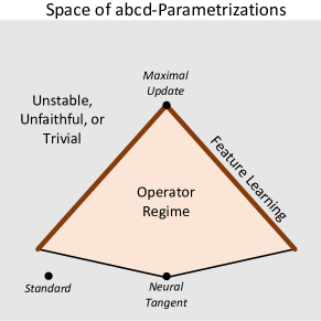
Figure 2.1: A Caricature of abcd-Parametrizations. The nontrivial stable faithful parametrizations form a high dimensional polyhedron. Those on a part of its boundary admit feature learning, while all others are in the operator regime. $\mu$P is a vertex in the former, while NTP, latter. The overall shape is similar to [45, Fig. 2]

The classification of abcd-parametrizations is similar to that of abc-parametrizations [45, Thm H.13]. We remind the reader that this holds for not only memoryless stationary but more generally memoryful nonstationary updates.

Theorem 2.8.19.

Adopt 2.8.2. Consider a nontrivial, stable, and faithful abcd-parametrization of an $L$-hidden layer MLP. Then

1. The following are equivalent to $r=0$

   1. feature learning

   2. feature learning in the $L$th layer

   3. feature kernels evolution

   4. feature kernel evolution in the $L$th layer

   5. prefeature learning

   6. prefeature learning in the $L$th layer

   7. prefeature kernels evolution

   8. prefeature kernel evolution in the $L$th layer

2. The following are equivalent to $r>0$

   1. the operator regime

   2. fixes all features

   3. fixes features in the $L$th layer

   4. fixes all feature kernels

   5. fixes feature kernel in the $L$th layer

   6. fixes all prefeatures

   7. fixes prefeatures in the $L$th layer

   8. fixes all prefeature kernels

   9. fixes prefeature kernel in the $L$th layer

3. If there is feature learning or feature kernel evolution or prefeature learning or prefeature kernel evolution in layer $l$, then there is feature learning and feature kernel evolution and prefeature learning and prefeature kernel evolution in layers $l,\ldots,L$.

4. If $r=0$, then $\bm{f}_{0}\xrightarrow{\mathrm{\mathrm{a.s.}}}0$ and $\bm{f}_{t}\xrightarrow{\mathrm{\mathrm{a.s.}}}\mathring{\bm{f}}_{t}$ for some deterministic $\mathring{\bm{f}}_{t}$. However, the converse is not true.

Consequently, we can generalize Dynamical Dichotomy to (nonlinear) entrywise updates.

Corollary 2.8.20 (Dynamical Dichotomy).

A nontrivial, stable, and faithful abcd-parametrization either admits feature learning or is in the operator regime, but not both.

Of course, the canonical examples here are $\mu$P in the feature learning regime and NTP in the operator regime. In the SGD case, LABEL:{thm:abcdclassification} and 2.8.20 are equivalent to their counterparts [45, Thm H.13, Cor H.14] other than a minor technical difference as discussed in 2.8.13.

Remark 2.8.21 (Maximality).

The $\mu$ and NT limits are resp. the “maximal” limits in the feature learning and operator regimes, in the sense that all parameter tensors contribute to the function update, and that any other limits in those regimes are just “downgrades” of $\mu$ and NT limits by zeroing out the initialization or learning rate of some parameters. See also 2.7.5.

Remark 2.8.22 (Pretraining is still futile in the operator regime even with adaptive optimizers).

[45, Thm H.17] holds almost verbatim in our case as well, after replacing “stable” with “stable and faithful” and “kernel regime” with “operator regime”: Finetuning any pretrained network in the operator regime would be equivalent to finetuning a randomly initialized network. Thus, pretraining in the operator regime is useless.

Remark 2.8.23 (Function Space Picture).

In the memoryless stationary case, an operator regime limit resides solely in the function space picture, i.e. $\bm{f}_{t+1}$ being solely determined by the function values $\bm{f}_{t}$ themselves (as opposed to the internal activations of $f$ as well) along with learning rate $\eta$ and error signals $\varepsilon_{t}$. However, as in [45, Remark 3.11], this is not true of any feature learning limit because one can construct counterexamples where $\bm{f}_{t}$ are close for two infinite-width limits but $\bm{f}_{t+1}$ are far.

Remark 2.8.24 (Not All Dynamics are Infinite-Width Limits).

Compared to the kernel regime in the SGD case, the operator regime now allows nonlinear evolution in the function space picture. Nevertheless, in such dynamics, $\bm{f}_{t+1}-\bm{f}_{t}$ must be linear in $\eta$ for every $t$. Thus, any function space evolution nonlinear in $\eta$ cannot be the infinite-width limit of any entrywise optimizer. For example, $\bm{f}_{t+1}-\bm{f}_{t}=-\eta\bm{f}_{t}-\eta^{2}\bm{f}_{t}^{2}$ is not a valid limit.

Remark 2.8.25 (Uniform Parametrization).

[45, Sec G] identified a subclass of abc-parametrizations, called uniform parametrizations, where all layers “learn the same amount of features” and the output layer is initialized and updated maximally. This is used in [40] to give an alternative presentation of $\mu$P as well as discussion of joint width-depth limit. This notion also makes sense for abcd-parametrizations: For every $s\in[0,\nicefrac{{1}}{{2}}]$, there is a unique stable and faithful abcd-parametrization, called UP_s such that $r_{l}=s$ for all $l=1,\ldots,L$ and $r_{L+1}=1$ and $a_{L+1}+b_{L+1}=1-s$. For example, UP₀ is $\mu$P and UP${}_{\nicefrac{{1}}{{2}}}$ is NTP.

2.9 Infinite-Width Limits for Any Architecture

Having written down the infinite-width limits of adaptive optimizers for MLPs, we now turn to general architectures. An astute reader may have already absorbed the key insights from the previous sections and can use them to derive the NT or $\mu$ limits for each new architecture in an ad hoc fashion. In contrast, here we describe the algorithm to do this once and for all, uniformly for all “reasonable” architectures. This uniformity of course requires abstraction, which is not conducive to quick comprehension; on the flip side, this algorithm will always be here for someone to fall back to if the ad hoc approach does not work out.

The main work here is not the proofs (which can be easily adapted from the MLP case and so are omitted), but the definitions: What is an architecture? What architecture counts as “reasonable”? How to define abcd-parametrization for any such architecture? What are their infinite-width limits? Answering these questions in the most generality requires careful thought.

2.9.1 Representating Architectures via Tensor Programs

Definition 2.9.1 (Architecture and Representability).

Let $\mathcal{T}_{n}=(\mathbb{R})^{j}\oplus(\mathbb{R}^{n})^{k}\oplus(\mathbb{R}^{n\times n})^{l}$. We shall call this the parameter space with $l$ matrix, $k$ vector, and $j$ scalar parameters.

A function family $f=\{f_{n}(-;-):\mathbb{R}^{d}\times\mathcal{T}_{n}\to\mathbb{R}^{e}\}_{n=1}^{\infty}$ (with fixed input and output dimensions $d$ and $e$ independent of $n$) is called an architecture. It has $l$ matrix, $k$ vector, and $j$ scalar parameters.

We say an architecture $f$ is representable if there is a $\textsc{Ne}{\otimes}\textsc{or}\top$ program $\pi$ and vectors $x^{1},\ldots,x^{e}$ in $\pi$ such that 1) $\pi$ has $j+d$ initial scalars, $k$ initial vectors, and $l$ initial matrices; and 2) for any $n$, when they are instantiated with $\xi\in(\mathbb{R})^{d}$ and $\Theta\in\mathcal{T}_{n}$, the sum of $x^{i}$’s entries yields $f_{n}(\xi;\Theta)_{i}$ for each $i\in[{e}]$. In this case, $(\pi,x^{1},\ldots,x^{e})$ is called a representation of $f$, and $\pi$ is called a representation program of $f$.

As demonstrated in [41, 43], 2.9.1 covers essentially every architecture in practice: RNNs, residual network, transformers, etc.

Remark 2.9.2.

In this definition, only the symbolic structure of the program matters; the random sampling of 2.6.3 and 2.6.4 plays no role.

Remark 2.9.3.

For simplicity, we only considered the case when the notion of “width” is the same throughout the network. Nevertheless, this definition can be easily modified to cover the nonuniform case, but stating it would be much more complex.

Remark 2.9.4.

In truth, we could have phrased 2.9.1 using $\textsc{Netsor}\top$ instead of $\textsc{Ne}{\otimes}\textsc{or}\top$, since we do not know of any neural network in the wild that is not $\textsc{Netsor}\top$-representable ($\textsc{Ne}{\otimes}\textsc{or}\top$ is only required for expressing adaptive optimization like Adam). But there is little cost in stating the more general version, which can potentially matter in the future.

Remark 2.9.5.

[46] also defined a notion of representable functions using $\textsc{Netsor}\top$. In comparison, our definition is much more general: Beyond the superficial difference of $\textsc{Ne}{\otimes}\textsc{or}\top$ here vs $\textsc{Netsor}\top$ there, [46] dealt with input and output layer weights in special ways, whereas here we do not, instead opting to uniformly deal with scalar, vector, and matrix parameters. The input and output weights of [46] are vector parameters in this view.

Example 2.9.6.

The $L$-hidden-layer MLP in Eq. 2.3 has $d+1$ vector parameters (where $d$ corresponds to input dimension and $1$ corresponds to output dimension) and $L-1$ matrix parameters. It is represented by the program that generates 1) $h^{1}$ using OuterNonlin and $h^{l},l\geq 2,$ using MatMul; 2) $x^{l}$ using OuterNonlin; and 3) generate function output by summing $W^{L+1}\odot x^{L}$ (so we can take $x^{1}$ in 2.9.1 to be $W^{L+1}\odot x^{L}$).

2.9.2 abcd-Parametrization for Any Architecture

Definition 2.9.7 (abcd-Parametrization for Representable Architectures).

Consider a representable architecture with representation program $\pi$. Fix a set of update functions $\bm{Q}=\{Q^{W}_{t}:\mathbb{R}^{t+1}\to\mathbb{R}\}_{t\geq 0,W}$ where $W$ ranges over every matrix, vector, and scalar parameters. An abcd-parametrization of this architecture is specified by $a_{W},b_{W},c_{W},d_{W}$ for each such $W$, along with an additional number $a_{\mathrm{out}}$, such that

1. We parametrize $W$ as $W=n^{-a_{W}}w$ for actual trainable parameter $w$;

2. We initialize each entry of $w$ iid from $\mathcal{N}(0,n^{-2b_{W}})$;

3. The learning rate is $\eta n^{-c_{W}}$ for some width-independent $\eta$;

4. The gradients of $w$ are multiplied by $n^{d_{W}}$ before being processed by $Q^{W}_{t}$: i.e., the update at time $t$ is

   $$w\leftarrow w-\eta n^{-c_{W}}Q^{W}_{t}(n^{d_{W}}g_{0},\ldots,n^{d_{W}}g_{t})$$

   where $g_{s},s=0,\ldots,t$, are the gradients of $w$ at time $s$ and $Q^{W}_{t}$ is applied entrywise;

and the function output is multiplied by $n^{-a_{\mathrm{out}}}$.

Remark 2.9.8.

In the MLP case, the $a_{\mathrm{out}}$ was absorbed into $a_{L+1}$. But in the generality of 2.9.1, output weights are not singled out, so we need to separately specify $a_{\mathrm{out}}$.

Remark 2.9.9.

As always, we are only concerned with scaling with $n$ here, but there can be a tunable constant hyperparameter in front of every power of $n$ in 2.2.1.

Remark 2.9.10.

The random initialization in 2.9.7 is always mean-zero. For some applications, such as layernorm/batchnorm weights $W$ (that is initialized as all 1s), this may seem insufficient. However, one can just refactor the parameter: For this particular example, we can refactor $W=1+W^{\prime}$ where $W^{\prime}$ is the initial vector of the program $\pi$. $W^{\prime}$ can then be initialized as $\mathcal{N}(0,\sigma n^{-2b_{W^{\prime}}})$ for some tunable constant hyperparameter $\sigma$ (which is set to 0 by practitioners typically).

NTP and $\mu$P naturally generalize to general representable architectures.

Definition 2.9.11 (NTP for general architecture).

For any representable architecture, its Neural Tangent Parametrization (NTP) is defined by the following setting of $a,b,c,d$ for matrix, vector, and scalar parameters as well as the output multiplier $a_{\mathrm{out}}$.

	matrix	vector	scalar	out
$a$	$\nicefrac{{1}}{{2}}$	$0$	$0$	$\nicefrac{{1}}{{2}}$
$b$	$0$	$0$	$0$	-
$c$	$1$	$\nicefrac{{1}}{{2}}$	$0$	-
$d$	$1$	$\nicefrac{{1}}{{2}}$	$0$	-

Definition 2.9.12 ($\mu$P for general architecture).

For any representable architecture, its Maximal Update Parametrization ($\mu$P) is defined by the following setting of $a,b,c,d$ for matrix, vector, and scalar parameters as well as the output multiplier $a_{\mathrm{out}}$.

	matrix	vector	scalar	out
$a$	$0$	$0$	$0$	$1$
$b$	$\nicefrac{{1}}{{2}}$	$0$	$0$	-
$c$	$1$	$0$	$0$	-
$d$	$1$	$1$	$0$	-

Remark 2.9.13.

In comparison to their counterparts for MLP, the NTP and $\mu$P above consider scalar parameters (which are not present in the MLP in Eq. 2.3). Otherwise, 2.4.1 can be recovered from 2.9.11 by mapping the columns $[2,L]$ to “matrix,” $1$ to “vector,” and $L+1$ to “vector” but with the value of $a$ taken from the “out” column. 2.5.1 can be recovered likewise from 2.9.12.

Before we formulate their limits, we need to discuss how to construct the “backpropagation” of an arbtrary of $\textsc{Ne}{\otimes}\textsc{or}\top$ program.

2.9.3 Interlude: Backpropagation and Total Programs

Recall that when $x\in\mathbb{R}^{n}$, the notation $\langle x_{\alpha}\rangle_{\alpha}$ denotes its average entry; this applies more generally to tensors, such as $\langle x_{\alpha_{1}\ldots\alpha_{r}}\rangle_{\alpha_{1}\cdots\alpha_{r}}$ when $x\in\mathbb{R}^{n\times\cdots\times n}=(\mathbb{R}^{n})^{\otimes r}$.

Definition 2.9.14 (Backpropagation Program).

Consider any $\textsc{Ne}{\otimes}\textsc{or}\top$ program $\pi$ and a vector $x$ in $\pi$. Then $\pi$’s backpropagation program wrt $x$ is an extension of $\pi$ defined by constructing the following objects on top of $\pi$: (Intuitively, one should interpret $d^{x}y=n\frac{\partial\langle x_{\alpha}\rangle_{\alpha}}{\partial y}$ if $y$ is a vector and $d^{x}c=\frac{\partial\langle x_{\alpha}\rangle_{\alpha}}{\partial c}$ if $c$ is a scalar.)

• $d^{x}x:=1_{n}\in\mathbb{R}^{n}$

• For any MatMul instruction $z:=Wy$ in $\pi$, we construct $d^{x|z}y:=W^{\top}d^{x}z$ (via another MatMul)

• For any Avg instruction $c:=\langle z_{\alpha}\rangle_{\alpha}$ in $\pi$, we construct $d^{x|c}z:=(d^{x}c){1}_{n}\in\mathbb{R}^{n}$ (via OuterNonlin)

• Suppose $y=\langle\psi(\bm{x};\bm{x}_{\beta_{1}};\cdots;\bm{x}_{\beta_{r}};\bm{c})\rangle_{\beta_{1}\cdots\beta_{r}}$. For each $i=0,\ldots,r$, let

  $$\bm{g}^{i}_{\beta_{0}\cdots\beta_{r}}=d^{x}y_{\alpha}\bm{\psi}_{i}(\bm{x}_{\beta_{0}};\cdots;\bm{x}_{\beta_{r}};\bm{c})\in\mathbb{R}^{|\bm{x}|},$$

  where $\bm{\psi}_{i}:\mathbb{R}^{|\bm{x}|(r+1)+l}\to\mathbb{R}^{|\bm{x}|}$ yields the derivative of $\psi$ against $\bm{x}$ in the $i$th slot. When $i=r+1$, we make the analogous definition for $\bm{g}^{r+1}_{\beta_{0}\cdots\beta_{r}}\in\mathbb{R}^{|\bm{c}|}$. We write ${\bm{\beta}}=(\beta_{0},\ldots,\beta_{r})$, ${\bm{\beta}}[i\mapsto\alpha]=(\beta_{0},\ldots,\beta_{i-1},\alpha,\beta_{i+1},\ldots,\beta_{r})$, and ${\bm{\beta}}_{-i}=(\beta_{0},\ldots,\beta_{i-1},\beta_{i+1},\ldots,\beta_{r})$. Then we construct $d^{x|y}\bm{c}=(d^{x|y}c^{1},\ldots,d^{x|y}c^{|\bm{c}|})$ and $d^{x|y}\bm{x}=(d^{x|y}x^{1},\ldots,d^{x|y}x^{|\bm{x}|})$ by

  $$d^{x|y}\bm{c} :=\langle\bm{g}^{r+1}_{\bm{\beta}}\rangle_{\bm{\beta}}\in\mathbb{R}^{|\bm{c}|}$$ OuterNonlin + Avg

  $$d^{x|y}\bm{x}_{\alpha} :=\sum_{i=0}^{r}\langle\bm{g}^{i}_{{\bm{\beta}}[i\mapsto\alpha]}\rangle_{{\bm{\beta}}_{-i}}\in\mathbb{R}^{|\bm{x}|}$$

  Explicitly,

  $$d^{x|y}\bm{x}_{\alpha}=\langle\bm{g}^{0}_{\alpha\beta_{1}\cdots\beta_{r}}\rangle_{\beta_{1}\cdots\beta_{r}}+\langle\bm{g}^{1}_{\beta_{0}\alpha\beta_{2}\cdots\beta_{r}}\rangle_{\beta_{0}\beta_{2}\cdots\beta_{r}}+\cdots+\langle\bm{g}^{r}_{\beta_{0}\cdots\beta_{r-1}\alpha}\rangle_{\beta_{0}\cdots\beta_{r-1}}$$

• Finally, for every vector or scalar $y$ in $\pi$ other than $x$,

  $$d^{x}y:=\sum_{u}d^{x|u}y$$

  where $u$ ranges over all vector or scalar in $\pi$ whose construction used $y$.

The subprogram constructing all of these new objects is denoted $d^{x}\pi$ (so that the backpropagation program is $\pi|d^{x}\pi$).

Recall ([44, Defn I.1]) that “$|$” (as in “$\pi|\pi^{\prime}$”) signifies the concatenation of programs.

Remark 2.9.15.

If $r=0$ in OuterNonlin (i.e., we just have a Nonlin+ instruction), then the formulas simplify to

$$d^{x|y}\bm{c} :=\langle d^{x}y_{\alpha}\bm{\psi}_{1}(\bm{x}_{\alpha};\bm{c})\rangle_{\alpha}$$

$$d^{x|y}\bm{x}_{\alpha} :=y_{\alpha}\bm{\psi}_{0}(\bm{x}_{\alpha};\bm{c}).$$

Definition 2.9.16 (Total Program $\bm{d}\bm{\pi}$).

Consider a representable architecture $f$ with representation $(\pi,x^{1},\ldots,x^{e})$. Gather all of $\pi$’s backpropagation programs wrt $x^{i}$ into a single (large) program:

$$\bm{d}\pi\mathrel{\raisebox{-1.29167pt}{$\mathbin{\overset{\text{{def}}}{=}}$}}\pi|d^{x^{1}}\pi|\cdots|d^{x^{e}}\pi.$$

Let $\xi\in\mathbb{R}^{d}$ be an input to $f$. Then $\bm{d}\pi(\xi)$ will denote the program $\bm{d}\pi$ with $\xi$ inserted as the appropriate initial scalars (c.f. 2.9.1). As in Section 2.3, we consider a set of $\mathcal{M}$ inputs $\bm{\xi}=\{\xi^{1},\ldots,\xi^{\mathcal{M}}\}\subseteq\mathbb{R}^{d}$. Then we set

$$\bm{d}\bm{\pi}\mathrel{\raisebox{-1.29167pt}{$\mathbin{\overset{\text{{def}}}{=}}$}}\bm{d}\pi(\xi^{1})|\cdots|\bm{d}\pi(\xi^{\mathcal{M}}),$$

whose initial data are the $j$ scalars, $k$ vectors, and $l$ matrices corresponding to $\mathcal{T}_{n}$ in 2.9.1; they are shared among all subprograms $\bm{d}\pi(\xi^{i})$. We call $\bm{d}\bm{\pi}$ the total program of $f$.

For any vector $y$ in $\pi$, we write $\bm{y}=(y(\xi^{1}),\ldots,y(\xi^{\mathcal{M}}))\in\mathbb{R}^{n\times\mathcal{M}}$ to denote the multi-vector of its counterparts in $\bm{d}\bm{\pi}$. We also write $\bm{d}\bm{y}=(d^{x^{j}}y(\xi^{a}))_{j\in[e],a\in[\mathcal{M}]}\in\mathbb{R}^{n\times e\times\mathcal{M}}$ for the multi-vector in $\bm{d}\bm{\pi}$ of its error signals.

2.9.4 Training Setup

The setup in Section 2.3 is defined with the MLP in mind, but can be generalized easily to deal with general architectures, as we do here for clariy: 1) Because we consider multi-dimensional outputs here, the error signal functions $\varepsilon_{t}$ obviously need to take the more general signature $\varepsilon_{t}:\mathbb{R}^{e\times\mathcal{M}}\to\mathbb{R}^{e\times\mathcal{M}}$. 2) The update functions $\bm{Q}$ now contain a $Q^{\Theta}_{t}:\mathbb{R}^{t+1}\to\mathbb{R}$ for every matrix, vector, and scalar parameter $\Theta$. Memoryless still means $Q^{\Theta_{t}}$ only depends on its last argument, and stationary still means $Q^{\Theta}_{t}$ is the same regardless of $\Theta$ and $t$. 3) The smoothness assumption we require is the natural adaptation of 2.3.2:

Assumption 2.9.17 (Smoothness).

Assume $\varepsilon_{t}$ and $Q^{\Theta}_{t}$ for all $\Theta,t$ are pseudo-Lipschitz and all nonlinearities used in the representing program has pseudo-Lipschitz derivatives.

2.9.5 Neural Tangent Limit

Memoryless Stationary Case

Definition 2.9.18 (Neural Tangent Operator for General Architecture).

Fix a representable architecture $f$ with representation $(\pi,x^{1},\ldots,x^{e})$. For any function $Q:\mathbb{R}\to\mathbb{R}$, we define the neural tangent $Q$-operator $\mathcal{K}_{Q}:\mathbb{R}^{e\times\mathcal{M}}\to\mathbb{R}^{e\times\mathcal{M}}$ by the following: for any $\bm{\chi}\in\mathbb{R}^{e\times\mathcal{M}}$,

$$\mathcal{K}_{Q}^{W}(\bm{\chi}) \mathrel{\raisebox{-1.29167pt}{$\mathbin{\overset{\text{{def}}}{=}}$}}\mathrm{Diag}_{\mathcal{M}}\sum_{\begin{subarray}{c}h=Wz\\ g=Wy\end{subarray}}\langle{\bm{d}\bm{g}}\overline{\hstretch{0.7}{\talloblong}\bm{d}\bm{h}\rangle{}_{\bm{\chi}}\langle\bm{z}\hstretch{0.7}{\talloblong}}{\bm{y}}\rangle$$ (2.32)

$$\mathcal{K}_{Q}^{v}(\bm{\chi}) \mathrel{\raisebox{-1.29167pt}{$\mathbin{\overset{\text{{def}}}{=}}$}}\langle{\bm{d}\bm{v}}\overline{\hstretch{0.7}{\talloblong}\bm{d}\bm{v}\rangle\cdot\bm{\chi}}$$ (2.33)

$$\mathcal{K}_{Q}(\bm{\chi}) \mathrel{\raisebox{-1.29167pt}{$\mathbin{\overset{\text{{def}}}{=}}$}}\sum_{W}\mathcal{K}_{Q}^{W}(\bm{\chi})+\sum_{v}\mathcal{K}_{Q}^{v}(\bm{\chi})$$ (2.34)

where the “bar” notation abbreviates application of $Q$ as in Eq. 1.2 and all kets and bras are evaluated in $\bm{d}\bm{\pi}$ (2.9.16) via 2.6.5. To interpret these formulas, we need to tell you two things:

1) Ranges of arguments. Here, $W$ ranges over all matrix parameters and $v$ over all vector parameters of $f$, and all kets are calculated from $\bm{d}\bm{\pi}$ by sampling matrix parameters from $\mathcal{N}(0,1/n)$ and vector parameters from $\mathcal{N}(0,1)$. The sum in Eq. 2.32 sums over all vectors $h,z,g,y$ in $\pi$ satisfying $h=Wz$ and $g=Wy$ (potentially $h=g$ and $z=y$).

2) Tensor operations. Here $\hstretch{0.7}{\talloblong}\bm{d}\bm{g}\rangle,\hstretch{0.7}{\talloblong}\bm{d}\bm{h}\rangle,\bm{\chi}\in\mathbb{R}^{e\times\mathcal{M}}$ while $\hstretch{0.7}{\talloblong}\bm{z}\rangle,\hstretch{0.7}{\talloblong}\bm{y}\rangle\in\mathbb{R}^{\mathcal{M}}$. First, we take the convention that each bra has the same shape as the corresponding ket: $\langle\bm{d}\bm{g}\hstretch{0.7}{\talloblong},\langle\bm{d}\bm{h}\hstretch{0.7}{\talloblong}\in\mathbb{R}^{e\times\mathcal{M}}$. Second, the meaning of $\hstretch{0.7}{\talloblong}\bm{d}\bm{h}\rangle{}_{\bm{\chi}}\langle\bm{z}\hstretch{0.7}{\talloblong}$ is

$$\hstretch{0.7}{\talloblong}\bm{d}\bm{h}\rangle{}_{\bm{\chi}}\langle\bm{z}\hstretch{0.7}{\talloblong}=\sum_{a\in[\mathcal{M}],i\in[e]}\chi^{ai}\hstretch{0.7}{\talloblong}d^{x^{i}}h(\xi^{a})\rangle\langle z(\xi^{a})\hstretch{0.7}{\talloblong}$$ (2.35)

(i.e., contraction of all matching indices), which generalizes the case of $e=1$ in 2.9.19. Likewise, in Eq. 2.33, $\hstretch{0.7}{\talloblong}\bm{d}\bm{v}\rangle\cdot\bm{\chi}\in\mathbb{R}$ contracts all indices. Finally, $\mathrm{Diag}_{\mathcal{M}}$ in Eq. 2.32 takes its argument tensor of shape $e\times\mathcal{M}\times\mathcal{M}$ and returns a tensor of shape $e\times\mathcal{M}$ by “taking the diagonal over the $\mathcal{M}$ dimension.”

Theorem 2.9.19 (Neural Tangent Limit for General Architecture).

Consider a representable architecture $f$ with representation $(\pi,x^{1},\ldots,x^{e})$ and any training routine in NTP (2.9.11) with memoryless stationary update function $Q$. Adopt 2.9.17. Further assume

1. $f$ has no scalar parameters, and

2. $\langle 1\hstretch{0.7}{\talloblong}x^{i}(\xi)\rangle=0$ for every input $\xi$ and output index $i\in[e]$ at initialization.

Recall $\bm{f}_{t}$ denotes the function after $t$ steps of updates from random initialization. Then

$$\bm{f}_{0}\xrightarrow{\mathrm{d}}\mathcal{N}(0,\langle\bm{x}\hstretch{0.7}{\talloblong}\bm{x}\rangle)$$

where $\bm{x}$ is the multi-vector consisting of $x^{1},\ldots,x^{e}$ evaluated on all $\mathcal{M}$ inputs. Additionally, for every $t\geq 0$, $\bm{f}_{t}$ converges almost surely to a random function $\mathring{\bm{f}_{t}}\in\mathbb{R}^{e\times\mathcal{M}}$ satisfying

$$\mathring{\bm{f}}_{s+1}-\mathring{\bm{f}}_{s} =-\eta\mathcal{K}_{Q}(\varepsilon_{s}(\mathring{\bm{f}}_{s})),\quad\text{for all $s$}.$$ (2.36)

Remark 2.9.20.

Note Simple GIA Check [43] may not be satisfied in general architectures, so that we cannot necessarily calculate kets like $\hstretch{0.7}{\talloblong}\bm{d}\bm{h}\rangle$ by assuming matrix parameters and their transposes are independent (even if no transposes occur in $\pi$), e.g., ignoring $\hstretch{0.7}{\talloblong}\bm{d}\bm{h}\dot{\rangle\mkern-3.0mu}\mkern 3.0mu$ in our calculations. Nevertheless, 2.9.19 still holds if one calculates $\hstretch{0.7}{\talloblong}\bm{d}\bm{h}\rangle$ correctly using the rules of 2.6.5.

Remark 2.9.21.

Assumption 39 ($\bm{x}$ being mean zero) in 2.9.19 is obviously necessary for us to arrive at a Gaussian Process limit at initialization. Assumption 1 is also necessary for two reasons: 1) at initialization, random initialization of scalar parameters would make the initial process a mixture of Gaussian processes (or a GP conditioned on the values of scalar parameters). Even if the scalar parameters are deterministic, the gradient wrt scalar parameters will also be a random process (possibly correlated to the process of the function) at initialization. 2) Function space picture (c.f. 2.8.23 and [45, Remark 3.11]) would no longer hold: One cannot track the evolution of the $\mathring{f}_{t}$ solely by knowing what it is at time $t=0$. Instead, one would need to track the values of the scalar parameters and their gradients as well. So in a sense we will have a “function space + scalar parameters” picture. The complete evolution of $\mathring{f}_{t}$ can then be described by a) the joint process of the function output, scalar parameters, and their gradients at initialization, together with b) an evolution equation involving how they evolve given their previous values in time. This is similar to [24].

Memoryful Nonstationary Case

As before, with some more notation we can write down the NT limit for any representable architecture.

Definition 2.9.22 (Neural Tangent Operator, Memoryful Nonstationary Case).

For memoryless but nonstationary update functions $\bm{Q}_{t}=\{Q^{\theta}_{t}:\mathbb{R}\to\mathbb{R}:\text{parameter }\theta\}$, we define $\mathcal{K}_{\bm{Q}_{t}}:\mathbb{R}^{e\times\mathcal{M}}\to\mathbb{R}^{e\times\mathcal{M}}$ with the same equation as Eqs. 2.32, 2.33 and LABEL:{eqn:KQgeneral}, except the bar notation abbreviates $Q^{W}_{t}$ or $Q^{v}_{t}$.

For general update functions $\bm{Q}_{t}=\{Q^{\theta}_{t}:\mathbb{R}^{t+1}\to\mathbb{R}\}_{\theta}$, we define $\mathcal{K}_{\bm{Q}_{t}}:\mathbb{R}^{(t+1)\times e\times\mathcal{M}}\to\mathbb{R}^{e\times\mathcal{M}}$,

$$\mathcal{K}_{\bm{Q}_{t}}^{W}(\bm{\chi}_{0},\ldots,\bm{\chi}_{t}) \mathrel{\raisebox{-1.29167pt}{$\mathbin{\overset{\text{{def}}}{=}}$}}\mathrm{Diag}_{\mathcal{M}}\sum_{\begin{subarray}{c}h=Wz\\ g=Wy\end{subarray}}\langle{\bm{d}\bm{g}}\overline{\hstretch{0.7}{\talloblong}\bm{d}\bm{h}\rangle{}_{\bm{\chi}_{\leq t}}\langle\bm{z}\hstretch{0.7}{\talloblong}}{\bm{y}}\rangle$$ (2.37)

$$\mathcal{K}_{\bm{Q}_{t}}^{v}({\bm{\chi}_{0},\ldots,\bm{\chi}_{t}}) \mathrel{\raisebox{-1.29167pt}{$\mathbin{\overset{\text{{def}}}{=}}$}}\langle{\bm{d}\bm{v}}\overline{\hstretch{0.7}{\talloblong}\bm{d}\bm{v}\rangle\cdot\bm{\chi}_{\leq t}}$$ (2.38)

$$\mathcal{K}_{\bm{Q}_{t}}(\bm{\chi}_{0},\ldots,\bm{\chi}_{t}) \mathrel{\raisebox{-1.29167pt}{$\mathbin{\overset{\text{{def}}}{=}}$}}\sum_{W}\mathcal{K}_{\bm{Q}_{t}}^{W}(\bm{\chi}_{0},\ldots,\bm{\chi}_{t})+\sum_{v}\mathcal{K}_{\bm{Q}_{t}}^{v}(\bm{\chi}_{0},\ldots,\bm{\chi}_{t})$$ (2.39)

where $\overline{\hstretch{0.7}{\talloblong}\bm{d}\bm{h}\rangle{}_{\bm{\chi}_{\leq t}}\langle\bm{z}\hstretch{0.7}{\talloblong}}$ is shorthand for $Q^{W}_{t}\left(\hstretch{0.7}{\talloblong}\bm{d}\bm{h}\rangle{}_{\bm{\chi}_{0}}\langle\bm{z}\hstretch{0.7}{\talloblong},\ldots,\hstretch{0.7}{\talloblong}\bm{d}\bm{h}\rangle{}_{\bm{\chi}_{t}}\langle\bm{z}\hstretch{0.7}{\talloblong}\right)$ and $\overline{\hstretch{0.7}{\talloblong}\bm{d}\bm{v}\rangle\cdot\bm{\chi}_{\leq t}}$ is shorthand for $Q^{v}_{t}\left(\hstretch{0.7}{\talloblong}\bm{d}\bm{v}\rangle\cdot\bm{\chi}_{0},\ldots,\hstretch{0.7}{\talloblong}\bm{d}\bm{v}\rangle\cdot\bm{\chi}_{t}\right)$

With this in mind, the following theorem yields the NT limit of Adam (Eq. $\mathtt{Adam}$) as a corollary.

Theorem 2.9.23 (Neural Tangent Limit, Memoryful Nonstationary Case).

If the update functions $\bm{Q}$ are memoryless but not necessarily stationary, then 2.9.19 holds with Eq. 2.36 replaced by

$$\mathring{\bm{f}}_{t+1}-\mathring{\bm{f}}_{t}=-\eta\mathcal{K}_{\bm{Q}_{t}}(\varepsilon_{t}(\mathring{\bm{f}}_{t})),\quad\text{for all $t$}.$$ (2.40)

For general $\bm{Q}$, not necessarily memoryless, 2.9.19 holds with Eq. 2.36 replaced by

$$\mathring{\bm{f}}_{t+1}-\mathring{\bm{f}}_{t}=-\eta\mathcal{K}_{\bm{Q}_{t}}(\varepsilon_{0}(\mathring{\bm{f}}_{0}),\ldots,\varepsilon_{t}(\mathring{\bm{f}}_{t})),\quad\text{for all $t$}.$$ (2.41)

2.9.6 Maximal Update Limit

Given a representable architecture, the representing program describes the symbolic procedure for computing the output of the network given an assignment of the input and parameters to concrete values. This procedure is well defined for any network width (by construction). Naturally, it remains well defined as explicitly spelled out below even when we “pass to the infinite-width limit.” In short, 2.9.24 specifies what it means for a program to compute something given an assignment of the input and parameters to concrete infinite-width limits (e.g., kets and operators).

Definition 2.9.24.

For any program $\pi$ and a vector $y$ in $\pi$, $\hstretch{0.7}{\talloblong}y\rangle$ can be thought of as a function, defined via 2.6.5, of $\{\hstretch{0.7}{\talloblong}W\hstretch{0.7}{\talloblong}\}_{W},\{\hstretch{0.7}{\talloblong}v\rangle\}_{v},\{\mathring{c}\}_{c}$ where $W,v,c$ range over the initial matrices, vectors, and scalars respectively. Consider an assignment $\Theta$ that assigns an operator ${\Theta\{W\}}$ to each initial matrix $W$, ket ${\Theta\{v\}}$ to each initial vector $v$, and a deterministic number $\Theta\{c\}$ to each initial scalar $c$. Then we write

$$\Theta\{\hstretch{0.7}{\talloblong}x\rangle{}_{\mathring{\bm{\chi}}}\langle y\hstretch{0.7}{\talloblong}\},\quad\Theta\{\hstretch{0.7}{\talloblong}y\rangle\},\quad\Theta\{\langle y\hstretch{0.7}{\talloblong}z\rangle\},\quad\Theta\{\mathring{\theta}\}$$

for $\hstretch{0.7}{\talloblong}x\rangle{}_{\mathring{\bm{\chi}}}\langle y\hstretch{0.7}{\talloblong},\hstretch{0.7}{\talloblong}y\rangle$, $\langle y\hstretch{0.7}{\talloblong}z\rangle$ and $\mathring{\theta}$ computed using this assignment (i.e., swapping out $\hstretch{0.7}{\talloblong}W\hstretch{0.7}{\talloblong}$ for $\Theta\{W\}$, $\hstretch{0.7}{\talloblong}v\rangle$ for $\Theta\{v\}$, and $\mathring{c}$ for $\Theta\{c\}$).

More precisely, we recursively define

$$\hstretch{0.7}{\talloblong}\Theta\{x\}\rangle \mathrel{\raisebox{-1.29167pt}{$\mathbin{\overset{\text{{def}}}{=}}$}}\Theta\{\hstretch{0.7}{\talloblong}x\rangle\}$$

$$\Theta\{\langle x\hstretch{0.7}{\talloblong}y\rangle\} \mathrel{\raisebox{-1.29167pt}{$\mathbin{\overset{\text{{def}}}{=}}$}}\langle\Theta\{x\}\hstretch{0.7}{\talloblong}\Theta\{y\}\rangle$$

$$\Theta\{\hstretch{0.7}{\talloblong}x\rangle{}_{\mathring{\bm{\chi}}}\langle y\hstretch{0.7}{\talloblong}\} \mathrel{\raisebox{-1.29167pt}{$\mathbin{\overset{\text{{def}}}{=}}$}}\hstretch{0.7}{\talloblong}\Theta\{x\}\rangle{}_{\Theta\{\mathring{\bm{\chi}}\}}\langle\Theta\{y\}\hstretch{0.7}{\talloblong}$$

$$\Theta\{\hstretch{0.7}{\talloblong}W\hstretch{0.7}{\talloblong}x\rangle\} \mathrel{\raisebox{-1.29167pt}{$\mathbin{\overset{\text{{def}}}{=}}$}}\hstretch{0.7}{\talloblong}\Theta\{W\}\hstretch{0.7}{\talloblong}\Theta\{x\}\rangle$$

$$\Theta\left\{\operatorname*{\mathbb{E}}_{\mathord{\ThisStyle{\LMpt\kern 1.0pt\LMpt\framebox{$\SavedStyle 1$}\kern 1.0pt\LMpt}}\cdots\mathord{\ThisStyle{\LMpt\kern 1.0pt\LMpt\framebox{$\SavedStyle r$}\kern 1.0pt\LMpt}}}\psi(\hstretch{0.7}{\talloblong}\bm{x}\rangle;\hstretch{0.7}{\talloblong}\bm{x}\rangle^{\mathord{\ThisStyle{\LMpt\kern 1.0pt\LMpt\framebox{$\SavedStyle 1$}\kern 1.0pt\LMpt}}};\cdots;\hstretch{0.7}{\talloblong}\bm{x}\rangle^{\mathord{\ThisStyle{\LMpt\kern 1.0pt\LMpt\framebox{$\SavedStyle r$}\kern 1.0pt\LMpt}}};\mathring{\bm{c}})\right\} \mathrel{\raisebox{-1.29167pt}{$\mathbin{\overset{\text{{def}}}{=}}$}}\operatorname*{\mathbb{E}}_{\mathord{\ThisStyle{\LMpt\kern 1.0pt\LMpt\framebox{$\SavedStyle 1$}\kern 1.0pt\LMpt}}\cdots\mathord{\ThisStyle{\LMpt\kern 1.0pt\LMpt\framebox{$\SavedStyle r$}\kern 1.0pt\LMpt}}}\psi(\hstretch{0.7}{\talloblong}\tilde{\bm{x}}\rangle;\hstretch{0.7}{\talloblong}\tilde{\bm{x}}\rangle^{\mathord{\ThisStyle{\LMpt\kern 1.0pt\LMpt\framebox{$\SavedStyle 1$}\kern 1.0pt\LMpt}}};\cdots;\hstretch{0.7}{\talloblong}\tilde{\bm{x}}\rangle^{\mathord{\ThisStyle{\LMpt\kern 1.0pt\LMpt\framebox{$\SavedStyle r$}\kern 1.0pt\LMpt}}};\Theta\{\mathring{\bm{c}}\})\quad\text{where $\tilde{\bm{x}}=\Theta\{\bm{x}\}$}$$

where we write $\hstretch{0.7}{\talloblong}\Theta\{W\}\hstretch{0.7}{\talloblong}=\Theta\{W\}$ for each initial matrix $W$, $\hstretch{0.7}{\talloblong}\Theta\{v\}\rangle=\Theta\{v\}$ for each initial vector $v$, and $\Theta\{\mathring{c}\}=\Theta\{c\}$ for each initial scalar $c$.

Memoryless Stationary Case

Theorem 2.9.25 ($\mu$-Limit for General Architecture).

Consider a representable architecture $f$ with representation $(\pi,x^{1},\ldots,x^{e})$ and any training routine in $\mu$P (2.9.12) with memoryless stationary update function $Q$. Adopt 2.9.17.

Then for each $t\geq 0$, $\bm{f}_{t}$ converges almost surely to $\mathring{\bm{f}}_{t}$ computed from the following.

1. (Forward and Backward Propagation) Let $\Theta_{t}$ be the assignment that assigns $\hstretch{0.7}{\talloblong}W_{t}\hstretch{0.7}{\talloblong}$ to each matrix parameter $W$, $\hstretch{0.7}{\talloblong}v\rangle$ to each vector parameter $v$, and $\mathring{c}_{t}$ to each scalar parameter $c$.

   $$\mathring{\bm{f}}_{t} =\Theta_{t}\{\langle 1\hstretch{0.7}{\talloblong}\bm{x}\rangle\}\in\mathbb{R}^{e\times\mathcal{M}} \mathring{\bm{\chi}}_{t} =\varepsilon_{t}(\mathring{\bm{f}}_{t})\in\mathbb{R}^{e\times\mathcal{M}}$$ (2.42)

   $$\hstretch{0.7}{\talloblong}\bm{y}_{t}\rangle =\Theta_{t}\{\hstretch{0.7}{\talloblong}\bm{y}\rangle\}\in\mathbb{R}^{\mathcal{M}} \hstretch{0.7}{\talloblong}\bm{d}\bm{y}_{t}\rangle =\Theta_{t}\{\hstretch{0.7}{\talloblong}\bm{d}\bm{y}\rangle\}\in\mathbb{R}^{e\times\mathcal{M}} y \pi$$ for any vector in (2.43)

   $$\mathring{\bm{a}}_{t} =\Theta_{t}\{\mathring{\bm{a}}\}\in\mathbb{R}^{\mathcal{M}} \bm{d}\mathring{\bm{a}}_{t} =\Theta_{t}\{\bm{d}\mathring{\bm{a}}\}\in\mathbb{R}^{e\times\mathcal{M}} a \pi$$ for any scalar in (2.44)

   Here $\bm{x}$ is the multi-vector consisting of $x^{1},\ldots,x^{e}$ evaluated on all $\mathcal{M}$ inputs, and all kets and limits are calculated in $\bm{d}\bm{\pi}$ via 2.6.5.

2. (Parameter Updates)

   $$\hstretch{0.7}{\talloblong}W_{t+1}\hstretch{0.7}{\talloblong} =\hstretch{0.7}{\talloblong}W_{t}\hstretch{0.7}{\talloblong}-\eta\overline{\sum_{h=Wx}\hstretch{0.7}{\talloblong}\bm{d}\bm{h}_{t}\rangle{}_{\mathring{\bm{\chi}}_{t}}\langle\bm{x}_{t}\hstretch{0.7}{\talloblong}} W$$ for every matrix parameter (2.45)

   $$\hstretch{0.7}{\talloblong}v_{t+1}\rangle =\hstretch{0.7}{\talloblong}v_{t}\rangle-\eta\overline{\hstretch{0.7}{\talloblong}\bm{d}v_{t}\rangle\cdot\mathring{\bm{\chi}}_{t}} v$$ for every vector parameter (2.46)

   $$\mathring{c}_{t+1} =\mathring{c}_{t}-\eta\overline{\bm{d}\mathring{c}_{t}} c$$ for every scalar parameter (2.47)

   where the tensor operations and summation over $h=Wx$ should be interpreted as in 2.9.18.

3. (Initialization) $\{\hstretch{0.7}{\talloblong}W_{0}\hstretch{0.7}{\talloblong}:\text{matrix parameter $W$}\}$ is a set of independent initial operators. Additionally,

   $$\hstretch{0.7}{\talloblong}v_{0}\rangle =\mathcal{N}(0,1) v$$ for every vector parameter (2.48)

   $$\mathring{c}_{0} \sim\mathcal{N}(0,1) c$$ for every scalar parameter (2.49)

   all independent from one another.

Here, we used the notation $W,v,c$ for matrix, vector, and scalar parameters, in contrast to $y$ and $a$ for vector and scalar generated by the program $\pi$. The former are exemplified by weights while the latter by (pre)activations.

Example 2.9.26.

In the MLP case with program $\pi$ given in Eq. 2.3, there are no generated scalars, so we can ignore Eq. 2.44. The generated vectors (in $\bm{d}\bm{\pi}$) are $\bm{h}^{1},\ldots,\bm{h}^{L}$ and $\bm{x}^{1},\ldots,\bm{x}^{L}$ as well as their error signals $d\bm{h}^{l},d\bm{x}^{l}$. So Eq. 2.43 reduces to the 2nd and 3rd rows in 2.7.1(1). Finally, the function output is given by averaging $w^{L+1}\odot x^{L}$, so the $\mathring{\bm{f}}_{t}=\Theta_{t}\{\langle 1\hstretch{0.7}{\talloblong}\bm{x}\rangle\}$ in Eq. 2.42 reduces to $\mathring{\bm{f}}_{t}=\langle w_{t}^{L+1}\hstretch{0.7}{\talloblong}\bm{x}^{L}_{t}\rangle$ in 2.7.1(1).

Remark 2.9.27 (Scalar Parameters).

In contrast to the NT limit (2.9.19), here we allow scalar parameters. The sampling of $\mathring{c}_{0}\sim\mathcal{N}(0,1)$ in Eq. 2.49 for every scalar parameter $c$ is just a consequence of the sampling in 2.9.7. But in fact for any deterministic initialization $C\in\mathbb{R}$ of $c$, we can set $\mathring{c}_{0}=C$ in Eq. 2.49, and 2.9.25 still holds. Indeed, for scalar parameters, the most natural initialization is probably either 0 (for additive parameters like bias) or 1 (for multiplicative parameters like layernorm weights). When scalar parameters have deterministic initializations, $\mathring{\bm{f}}_{t}$ is always deterministic as well; however, in 2.9.25, as written, $\mathring{\bm{f}}_{t}$ is only deterministic conditioned on $\mathring{c}_{0}$ for every scalar parameter $c$.

Remark 2.9.28 ($\mu$P is Most Natural).

As discussed in 2.7.2, $\mu$P is in a sense the most natural parametrization because its infinite-width limit is just a direct “ket-translation” of the finite-width computations, no matter the architecture. Compare this with NTP, where the Gaussian process and kernel behaviors can only happen under some relative restrictive conditions, like “no scalar parameters” (2.9.19 and 2.9.21).

Remark 2.9.29.

In the $\mu$-limit for a general architecture, $\mathring{\bm{f}}_{0}$ no longer needs to be 0, unlike 2.7.1. For example, if in an MLP with relu activation, the output is given by the average entry of the last layer activation vector, then obviously $\mathring{\bm{f}}_{0}$ will always be positive.

Memoryful Nonstationary Case

Theorem 2.9.30 ($\mu$-Limit for General Architecture, Memoryful Nonstationary Updates).

If $\bm{Q}$ is memoryless but not stationary, then 2.9.25 holds if the bars in LABEL:{eqn:muP_op_update_general}, LABEL:{eqn:muP_ket_update_general} and LABEL:{eqn:muP_scalar_update_general} are interpreted as $Q^{W}_{t},Q^{v}_{t},$ and $Q^{c}_{t}$.

If $\bm{Q}$ is not memoryless, then 2.9.25 holds if LABEL:{eqn:muP_op_update_general}, LABEL:{eqn:muP_ket_update_general} and LABEL:{eqn:muP_scalar_update_general} are replaced with

$$\hstretch{0.7}{\talloblong}W_{t+1}\hstretch{0.7}{\talloblong} =\hstretch{0.7}{\talloblong}W_{t}\hstretch{0.7}{\talloblong}-\eta\overline{\sum_{h=Wx}\hstretch{0.7}{\talloblong}\bm{d}\bm{h}_{\leq t}\rangle{}_{\mathring{\bm{\chi}}_{\leq t}}\langle\bm{x}_{\leq t}\hstretch{0.7}{\talloblong}} W$$ for every matrix parameter

$$\hstretch{0.7}{\talloblong}v_{t+1}\rangle =\hstretch{0.7}{\talloblong}v_{t}\rangle-\eta\overline{\hstretch{0.7}{\talloblong}\bm{d}v_{{\leq t}}\rangle\cdot\mathring{\bm{\chi}}_{{\leq t}}} v$$ for every vector parameter

$$\mathring{c}_{t+1} =\mathring{c}_{t}-\eta\overline{\bm{d}\mathring{c}_{\leq t}} c$$ for every scalar parameter

where the bar notations abbreviate

$$\overline{\sum_{h=Wx}\hstretch{0.7}{\talloblong}\bm{d}\bm{h}_{\leq t}\rangle{}_{\mathring{\bm{\chi}}_{\leq t}}\langle\bm{x}_{\leq t}\hstretch{0.7}{\talloblong}} =Q^{W}_{t}\left(\sum_{h=Wx}\hstretch{0.7}{\talloblong}\bm{d}\bm{h}_{0}\rangle{}_{\mathring{\bm{\chi}}_{0}}\langle\bm{x}_{0}\hstretch{0.7}{\talloblong},\ldots,\sum_{h=Wx}\hstretch{0.7}{\talloblong}\bm{d}\bm{h}_{t}\rangle{}_{\mathring{\bm{\chi}}_{t}}\langle\bm{x}_{t}\hstretch{0.7}{\talloblong}\right)$$

$$\overline{\hstretch{0.7}{\talloblong}\bm{d}v_{{\leq t}}\rangle\cdot\mathring{\bm{\chi}}_{{\leq t}}} =Q^{v}_{t}\left(\hstretch{0.7}{\talloblong}\bm{d}v_{{0}}\rangle\cdot\mathring{\bm{\chi}}_{{0}},\ldots,\hstretch{0.7}{\talloblong}\bm{d}v_{{t}}\rangle\cdot\mathring{\bm{\chi}}_{{t}}\right)$$

$$\overline{\bm{d}\mathring{c}_{\leq t}} =Q^{c}_{t}\left(\bm{d}\mathring{c}_{0},\ldots,\bm{d}\mathring{c}_{t}\right).$$

2.10 Extensions

2.10.1 Weight Decay

Consider the update equation (Eq. 2.4) with decoupled weight decay $\lambda$:

$$w^{l}_{t}=(1-\lambda)w^{l}_{t-1}-\eta n^{-c_{l}}Q_{t}^{l}(n^{d_{l}}g_{0},\ldots,n^{d_{l}}g_{t}).$$ (2.50)

This decoupled weight decay $\lambda$ is equivalent to a traditional weight decay value $\nicefrac{{\lambda}}{{\eta n^{-c_{l}}}}$. It’s obvious that $\lambda$ should be invariant to the width $n$: if $\lambda\to\infty$ with $n$, then $1-\lambda<0$ eventually; if $\lambda\to 0$ with $n$, then weight decay has no effect in the limit.

The theory in this section covers AdamW [27], SGD with weight decay, and so on.

Maximal Update Limit

2.7.1 holds with Eqs. 2.20, 2.21 and 2.22 replaced with

$$\hstretch{0.7}{\talloblong}w^{1}_{t+1}\rangle =(1-\lambda)\hstretch{0.7}{\talloblong}w^{1}_{t}\rangle-\eta\overline{\hstretch{0.7}{\talloblong}d\bm{h}_{t}^{1}\rangle_{\mathring{\bm{\chi}}_{t}}\bm{\xi}^{\top}}$$ (2.51)

$$\hstretch{0.7}{\talloblong}W^{l}_{t+1}\hstretch{0.7}{\talloblong} =(1-\lambda)\hstretch{0.7}{\talloblong}W^{l}_{t}\hstretch{0.7}{\talloblong}-\eta\overline{\hstretch{0.7}{\talloblong}d\bm{h}_{t}^{l}\rangle{}_{\mathring{\bm{\chi}}_{t}}\langle\bm{x}_{t}^{l-1}\hstretch{0.7}{\talloblong}},\ \forall l\in[2,L]$$ (2.52)

$$\hstretch{0.7}{\talloblong}w_{t+1}^{L+1}\rangle =(1-\lambda)\hstretch{0.7}{\talloblong}w_{t}^{L+1}\rangle-\eta\overline{\hstretch{0.7}{\talloblong}\bm{x}_{t}^{L}\rangle\cdot\mathring{\bm{\chi}}_{t}}.$$ (2.53)

All other $\mu$-limit theorems (2.5.2, 2.5.3, 2.7.3, and 2.9.30) hold with similar modifications. In particular, if we interpret the bars in Eqs. 2.51, 2.45 and 2.53 as Eq. $\mathtt{Adam}$ and replace the $\bullet_{t}$ subscripts under the bars to $\bullet_{\leq t}$ (c.f. the notation in 2.7.3), then we get the equations for AdamW’s $\mu$-limit.

Neural Tangent

Fix decoupled weight decay $\lambda$.

Definition 2.10.1.

For each $l=1,\ldots,L$ and $s=0,1,\ldots$, the ket $\hstretch{0.7}{\talloblong}\bm{h}^{l}_{s}\rangle\in\mathbb{R}^{\mathcal{M}}$ is constructed as a mean-zero Gaussian vector with covariance matrix $(1-\lambda)^{2s}\langle\bm{x}^{l-1}_{s}\hstretch{0.7}{\talloblong}\bm{x}^{l-1}_{s}\rangle$ when $l>1$ or $\bm{\xi}^{\top}\bm{\xi}$ when $l=1$. Simultaneously, $\bm{x}^{l}_{s}\mathrel{\raisebox{-1.29167pt}{$\mathbin{\overset{\text{{def}}}{=}}$}}\phi(\hstretch{0.7}{\talloblong}\bm{h}^{l}_{s}\rangle)\in\mathbb{R}^{\mathcal{M}}$ for $l=1,\ldots,L$. Furthermore, for any $s,t\geq 0$, $\hstretch{0.7}{\talloblong}\bm{h}^{l}_{s}\rangle$ and $\hstretch{0.7}{\talloblong}\bm{h}^{l}_{t}\rangle$ are jointly Gaussian with covariance $(1-\lambda)^{s+t}\langle\bm{x}^{l-1}_{s}\hstretch{0.7}{\talloblong}\bm{x}^{l-1}_{t}\rangle$.

Definition 2.10.2.

For each $l=L,\ldots,1$ and $s=0,1,\ldots$, the ket $\hstretch{0.7}{\talloblong}d\bm{x}^{l}_{s}\rangle\in\mathbb{R}^{\mathcal{M}}$ is independent from $\{\hstretch{0.7}{\talloblong}\bm{x}^{l}_{t}\rangle,\hstretch{0.7}{\talloblong}\bm{h}^{l}_{t}\rangle\}_{l=1}^{L}$ for any $t$ and is a mean-zero Gaussian vector with covariance matrix $(1-\lambda)^{2s}\langle d\bm{h}^{l+1}_{s}\hstretch{0.7}{\talloblong}d\bm{h}^{l+1}_{s}\rangle$ when $l<L$ or the all-1s matrix when $l=L$. Simultaneously, $\hstretch{0.7}{\talloblong}d\bm{h}^{l}_{s}\rangle\mathrel{\raisebox{-1.29167pt}{$\mathbin{\overset{\text{{def}}}{=}}$}}\phi^{\prime}(\hstretch{0.7}{\talloblong}\bm{h}^{l}_{s}\rangle)\odot\hstretch{0.7}{\talloblong}d\bm{x}^{l}_{s}\rangle\in\mathbb{R}^{\mathcal{M}}$ for all $l$. Furthermore, for any $s,t\geq 0$, $\hstretch{0.7}{\talloblong}d\bm{x}^{l}_{s}\rangle$ and $\hstretch{0.7}{\talloblong}d\bm{x}^{l}_{t}\rangle$ are jointly Gaussian with covariance $(1-\lambda)^{s+t}\langle d\bm{h}^{l+1}_{s}\hstretch{0.7}{\talloblong}d\bm{h}^{l+1}_{t}\rangle$.

Theorem 2.10.3.

With decoupled weight decay $\lambda$, 2.4.7 holds with the update equation Eq. 2.9 replaced by

$$\mathring{\bm{f}}_{t+1}-\mathring{\bm{f}}_{0} =-\eta\sum_{s=0}^{t}(1-\lambda)^{t-s}\mathrm{Diag}\sum_{l=1}^{L+1}\langle{d\bm{h}^{l}_{t+1}}\overline{\hstretch{0.7}{\talloblong}d\bm{h}^{l}_{s}\rangle{}_{\bm{\chi}_{s}}\langle\bm{x}^{l-1}_{s}\hstretch{0.7}{\talloblong}}{\bm{x}^{l-1}_{t+1}}\rangle.$$

For memoryless nonstationary updates, interpret the bar as $Q_{t}^{l}$. For memoryful nonstationary updates, replace the nonlinear outer product with $\overline{\hstretch{0.7}{\talloblong}d\bm{h}^{l}_{\leq s}\rangle{}_{\bm{\chi}_{\leq s}}\langle\bm{x}^{l-1}_{\leq s}\hstretch{0.7}{\talloblong}}$ (c.f. 2.7.3 for the notation).

Note that when $\lambda=0$, $\bm{h}^{l}_{s}$ is invariant to $s$ as are $\bm{x}^{l}_{s},d\bm{h}^{l}_{s},d\bm{x}^{l}_{s}$, and this exponentially weighted sum just reduces to a simple sum and thus to Eq. 2.9.

In the memoryful case, interpreting the bar in 2.10.3 as Eq. $\mathtt{Adam}$ yields the NT limit of AdamW. The limit theorems (2.9.19 and 2.9.23) for general architecture also hold with analogous modifications.

2.10.2 Update Clipping and Normalization

We now add update clipping or normalization to Eq. 2.50:

$$w^{l}_{t}=(1-\lambda)w^{l}_{t-1}-\eta n^{-c_{l}}\cdot\nu^{-1}Q_{t}^{l}(n^{d_{l}}g_{0},\ldots,n^{d_{l}}g_{t}),$$ (2.54)

where

• if we are doing update normalization, then we set $\nu\leftarrow\|Q_{t}^{l}(n^{d_{l}}g_{0},\ldots,n^{d_{l}}g_{t})\|$;

• if we are doing update clipping, then calculate additionally $\nu\leftarrow\min(\nu,\theta^{l})$ where $\theta^{l}$ is a threshold hyperparameter for layer $l$.

Some recent works [49, 35, 50, 6, 5, 26] normalize the update by the current weight (Frobenius) norm instead of by the update norm. We explore its implications in LABEL:{sec:normbycurrentweightnorm}. For now we focus on the formulation above.

The key questions we explore here are:

1. How should the abcd values adjust to update clipping and normalization?

2. What do the neural tangent and maximal update limits look like?

3. How should the threshold hyperparameter $\theta^{l}$ scale with width $n$?

The key intuition is as follows: In all “reasonable” parametrizations (more precisely, faithful ones (2.8.8)), $Q_{t}^{l}(n^{d_{l}}g_{0},\ldots,n^{d_{l}}g_{t})$ is entrywise $\Theta(1)$. Thus, its norm $\nu$ scales like $\sqrt{\#\text{entries}}$, as can be verified via the Master Theorem (2.6.10). For example, for the input and output weights of the MLP (Eq. 2.3), this is $\sqrt{n}$, while for the hidden weights, this is $n$. Therefore, for update clipping, the threshold should be

$$\theta^{l}=\theta^{l}_{0}n^{e_{l}}\quad\text{where}\quad e_{l}=\begin{cases}\nicefrac{{1}}{{2}}&\text{if $l=1,L+1$}\\ 1&\text{otherwise,}\end{cases}$$ (2.55)

for some tunable hyperparameter $\theta^{l}_{0}$ independent of width. Otherwise, either the clipping has no effect (if $\theta^{l}$ is larger than this) or $\nu$ after update clipping is always equal to the threshold $\theta^{l}$ (if $\theta^{l}$ is smaller than this).

At the same time, $c_{l}$ should be ${e_{l}}$ smaller than if there is no update normalization or clipping (i.e., the learning rate should be larger). Thus, for example,

Definition 2.10.4.

The NTP with update normalization or clipping is

$l$	$[2,L]$	$1$	$L+1$
$a_{l}$	$\nicefrac{{1}}{{2}}$	0	$\nicefrac{{1}}{{2}}$
$b_{l}$	$0$	$0$	$0$
$c_{l}$	$0$	$0$	$0$
$d_{l}$	$1$	$\nicefrac{{1}}{{2}}$	$\nicefrac{{1}}{{2}}$

where update clipping thresholds $\theta^{l}$ scale as in Eq. 2.55.

Definition 2.10.5.

The $\mu$P with update normalization or clipping is

$l$	$[2,L]$	$1$	$L+1$
$a_{l}$	$0$	$0$	$1$
$b_{l}$	$\nicefrac{{1}}{{2}}$	$0$	$0$
$c_{l}$	$0$	$-\nicefrac{{1}}{{2}}$	$-\nicefrac{{1}}{{2}}$
$d_{l}$	$1$	$1$	$1$

where update clipping thresholds $\theta^{l}$ scale as in Eq. 2.55.

Likewise, the classification of parametrizations in Section 2.8 hold for update normalization or clipping if we replace all mentions of $c_{l}$ in Section 2.8 with $c_{l}+e_{l}$. For example,

Definition 2.10.6.

With update clipping or normalization, we redefine

$$r_{l}\mathrel{\raisebox{-1.29167pt}{$\mathbin{\overset{\text{{def}}}{=}}$}}\begin{cases}c_{l}+e_{l}+a_{l}-1&\text{if $l>1$}\\ c_{l}+e_{l}+a_{l}&\text{if $l=1$}\end{cases},\quad r_{\leq l}\mathrel{\raisebox{-1.29167pt}{$\mathbin{\overset{\text{{def}}}{=}}$}}\min_{m=1}^{l}r_{l},\quad r\mathrel{\raisebox{-1.29167pt}{$\mathbin{\overset{\text{{def}}}{=}}$}}r_{\leq L}$$

Then $\bm{x}^{L}_{t}-\bm{x}^{L}_{0}=\Theta(n^{-r})$ still and it remains that $r=\nicefrac{{1}}{{2}}$ for NTP (2.10.4) and $r=0$ for $\mu$P (2.10.5) with the new definitions above.

General Architectures

For general architectures, there is one $e_{w}$ for every parameter tensor $w$, and should be set to $0,\nicefrac{{1}}{{2}},$ and $1$ respectively for scalar, vector, and matrix parameters. Then the obvious generalization of the above discussion holds.

Maximal Update Limit

Definition 2.10.7.

For any random vector $\bm{X}$, let $|\bm{X}|\mathrel{\raisebox{-1.29167pt}{$\mathbin{\overset{\text{{def}}}{=}}$}}\sqrt{\operatorname*{\mathbb{E}}\|\bm{X}\|^{2}}$. Then let $\tilde{\bm{X}}\mathrel{\raisebox{-1.29167pt}{$\mathbin{\overset{\text{{def}}}{=}}$}}\bm{X}/|\bm{X}|$.

Then 2.7.1 holds with Eqs. 2.20, 2.21 and 2.22 replaced with (essentially, compared to Eqs. 2.51, 2.52 and 2.53 we added a tilde $\tilde{\ }$ to all bars.)

$$\hstretch{0.7}{\talloblong}w^{1}_{t+1}\rangle =(1-\lambda)\hstretch{0.7}{\talloblong}w^{1}_{t}\rangle-\eta\tilde{\overline{\hstretch{0.7}{\talloblong}d\bm{h}_{t}^{1}\rangle_{{\bm{\chi}}_{t}}\bm{\xi}^{\top}}}$$ (2.56)

$$\hstretch{0.7}{\talloblong}W^{l}_{t+1}\hstretch{0.7}{\talloblong} =(1-\lambda)\hstretch{0.7}{\talloblong}W^{l}_{t}\hstretch{0.7}{\talloblong}-\eta\tilde{\overline{\hstretch{0.7}{\talloblong}d\bm{h}_{t}^{l}\rangle{}_{\bm{\chi}_{t}}\langle\bm{x}_{t}^{l-1}\hstretch{0.7}{\talloblong}}},\ \forall l\in[2,L]$$ (2.57)

$$\hstretch{0.7}{\talloblong}w_{t+1}^{L+1}\rangle =(1-\lambda)\hstretch{0.7}{\talloblong}w_{t}^{L+1}\rangle-\eta\tilde{\overline{\hstretch{0.7}{\talloblong}\bm{x}_{t}^{L}\rangle\cdot{\bm{\chi}}_{t}}}.$$ (2.58)

Here, we think of $\hstretch{0.7}{\talloblong}\bm{h}_{t}^{l}\rangle{}_{\mathring{\bm{\chi}}_{t}}\langle\bm{x}_{t}^{l-1}\hstretch{0.7}{\talloblong}$ as a scalar random variable with the same distribution as $\sum_{i=1}^{\mathcal{M}}\mathring{\chi}_{t}(\xi_{i})\hstretch{0.7}{\talloblong}h^{l}_{t}(\xi_{i})\rangle\hstretch{0.7}{\talloblong}x^{l-1}_{t}(\xi_{i})\rangle^{\mathord{\ThisStyle{\LMpt\kern 1.0pt\LMpt\framebox{$\SavedStyle 1$}\kern 1.0pt\LMpt}}}\in\mathbb{R}$.

If doing update clipping, then interpret $\tilde{\bm{X}}\mathrel{\raisebox{-1.29167pt}{$\mathbin{\overset{\text{{def}}}{=}}$}}\bm{X}/\min(\theta_{0},|\bm{X}|)$ for $\theta_{0}$ being the $\theta^{l}_{0}$ (Eq. 2.55) for appropriate layer $l$.

Similar statements hold for other $\mu$-limit theorems, including those in general architectures.

Neural Tangent Limit

2.10.3 holds with a tilde added to all bars, where the tilde should be interpreted according to $\tilde{\bm{X}}\mathrel{\raisebox{-1.29167pt}{$\mathbin{\overset{\text{{def}}}{=}}$}}\bm{X}/|\bm{X}|$ if doing update normalization or $\tilde{\bm{X}}\mathrel{\raisebox{-1.29167pt}{$\mathbin{\overset{\text{{def}}}{=}}$}}\bm{X}/\min(\theta_{0},|\bm{X}|)$ if doing update clipping. Similar statements hold for other NT limit theorems, including those in general architectures.

Normalization by Current Weight Norm

Now suppose in Eq. 2.54, we normalizd by the current weight norm instead, i.e.,

$$\nu\leftarrow\|w^{l}_{t-1}\|_{F}.$$

For simpicity, assume the weight decay $\lambda$ is zero; our conclusion will turn out to hold even when this is not the case.

Let’s consider what happens to the hidden weights. Consider $W^{l}$ for $l\in[2,L]$. The Frobenius norm of its initialization $W^{l}_{0}\in\mathbb{R}^{n\times n}$ (a random Gaussian matrix with $W_{\alpha\beta}\sim\mathcal{N}(0,1/n)$) scales like $\Theta(\sqrt{n})$ (in fact, asymptotically $\sqrt{n}+O(1)$). But, in a stable parametrization (2.8.7), the Frobenius norm of $\delta W^{l}_{t}=W^{l}_{t}-W^{l}_{t-1}$, a nonlinear outer product with $O(1/n)$ entries, scales like $O(1)$. This means that

$$\frac{\|\delta W^{l}_{t}\|_{F}}{\|W^{l}_{0}\|_{F}}=\frac{\|\delta w^{l}_{t}\|_{F}}{\|w^{l}_{0}\|_{F}}=O(1/\sqrt{n}).$$

Therefore,

$$\frac{\|W^{l}_{0}+\delta W^{l}_{1}+\cdots+\delta W^{l}_{t}\|_{F}}{\|W^{l}_{0}\|_{F}}=\frac{\|W^{l}_{t}\|_{F}}{\|W^{l}_{0}\|_{F}}=\frac{\|w^{l}_{t}\|_{F}}{\|w^{l}_{0}\|_{F}}\to 1$$

for any $t$ as $n\to\infty$. So $\nu=\|w^{l}_{t-1}\|_{F}=\Theta(\|w^{l}_{0}\|_{F})=\Theta(n^{1-b_{l}})$ (in fact, $\nu/n^{-b_{l}}\to 1$).

In contrast, for the input layer weight $W=W^{1}$, we have $\Delta W_{t}=O(W_{0})$ (entrywise and in Frobenius norm) in a stable parametrization. If the parametrization is furthermore faithful (2.8.8), then for $W=W^{L+1}$, this is true as well (c.f. 2.8.13). So $\|w^{1}_{t}\|_{F}/\|w^{1}_{0}\|_{F}$ and $\|w^{L+1}_{t}\|_{F}/\|w^{L+1}_{0}\|_{F}$ are both $\Theta(1)$ (but $\not\to 1$ generally) and $\nu=\Theta(n^{\nicefrac{{1}}{{2}}-b_{l}})$ in both cases.

Therefore, if we subtract $b_{l}$ from $e_{l}$ in Eq. 2.55, then all discussion above applies. For example, the parametrizations for current weight norm can be obtained by adding the $b_{l}$ row to the $c_{l}$ row.

Definition 2.10.8.

The NTP with update normalization or clipping with current weight norm is the same as 2.10.4.

Definition 2.10.9.

The $\mu$P with update normalization or clipping with current weight norm is

$l$	$[2,L]$	$1$	$L+1$
$a_{l}$	$0$	$0$	$1$
$b_{l}$	$\nicefrac{{1}}{{2}}$	$0$	$0$
$c_{l}$	$\nicefrac{{1}}{{2}}$	$-\nicefrac{{1}}{{2}}$	$-\nicefrac{{1}}{{2}}$
$d_{l}$	$1$	$1$	$1$

where the clipping thresholds $\theta^{l}$ scale as $n^{\nicefrac{{1}}{{2}}}$.

The limit equations for $\mu$P in this case is just Eqs. 2.56, 2.57 and 2.58 but with the tilde interpreted as dividing by $\sqrt{\langle w^{1}_{t}\hstretch{0.7}{\talloblong}w^{1}_{t}\rangle}$, $1$, and $\sqrt{\langle w^{L+1}_{t}\hstretch{0.7}{\talloblong}w^{L+1}_{t}\rangle}$ respectively. Similar modifications apply to the NT limits.

Likewise, the classification of parametrizations hold if we replace each $c_{l}$ with $c_{l}+e_{l}-b_{l}$.

We have assumed that the weight decay $\lambda$ is 0 at the beginning. In the general case, define $\delta W_{t}=W_{t}-(1-\lambda)W_{t-1}$ instead, but the same calculations will yield the same conclusions.

2.10.3 Second Moment Factoring ala Adafactor

The key observation here is that, even though the factored update function $Q$ is not entrywise anymore, the update itself is still a nonlinear outer product of $d\bm{h}_{\leq t}$ and $d\bm{x}_{\leq t}$ (with some scalars variables inserted in an appropriate $\textsc{Ne}{\otimes}\textsc{or}\top$ program), All of our theory in fact holds as-is for this more general kind of update function, since they all factor through the OuterNonlin instruction of $\textsc{Ne}{\otimes}\textsc{or}\top$.

2.10.4 Future Optimizers

As technology advances, we may get better optimizers of very different forms than we discussed here. But we can quite reasonably expect them to continue to efficiently utilize GPUs, i.e., perform large matrix-multiplies. As such, these optimizers can always be analyzed in a Tensor Program. So the lesson is: as long as one understands Tensor Programs, one can always derive the correct way of scaling an optimizer (with width).

2.11 Proof Sketch

$\textsc{Ne}{\otimes}\textsc{or}\top$ programs equipped with their Master Theorem (2.6.10) provide the main tool to all of our rigorous results. For example, to prove the neural tangent or $\mu$ limit equations, one can: express the optimization dynamics using a $\textsc{Ne}{\otimes}\textsc{or}\top$ program, mechanically compute the kets according to 2.6.5, and apply 2.6.10 to compute the limit (see full proofs in Sections 3.2 and 3.3). What remains is to prove 2.6.10 using a strategy which we now outline.

In a program, all vectors can be collected into an $n\times M$ matrix $V$ where $n$ is the dimension of each vector, and $M$ is the total number of vectors. The Master Theorem can be interpreted as saying that each row of $V$ (i.e., the slice for each $\alpha\in[n]$) is roughly an iid sample from some distribution $\mathcal{D}$ on $\mathbb{R}^{M}$ (the distribution of some multivariate ket computed from 2.6.5). Specifically, 2.6.10 and all previous versions of the Master Theorem formalize this by saying: this matrix $V$ of vectors looks similar to a matrix $V^{\prime}$ of iid samples from $\mathcal{D}$, as measured by applying arbitrary pseudo-Lipschitz “test function $\psi$” to both sides and taking averages (the scalars in 2.6.10 are exactly of this form by Avg).

Core Insight

Our core insight here is that $V$ is in fact similar to $V^{\prime}$ in a stronger sense without needing to refer to any test function $\psi$: There is a “small” matrix $\delta V$ of the same shape as $V$ such that $V-\delta V$ is distributed exactly the same as $V^{\prime}$. In general, if this happens, then we say $V$ is distributionally equivalent, or dequivalent, to $V^{\prime}$ (4.3.15). The definition of “small” roughly means that $\delta V$ is $\tilde{O}(1)$ in $L^{2}$ norm, so that dequivalence is morally just “close in Wasserstein distance.” This “Wasserstein” notion is a stronger sense of closeness of $V$ to $V^{\prime}$ than the “test function” notion described in the previous paragraph because the test function $\psi$ is (by assumption) smooth enough that $\delta V$ contributes a vanishing amount to the average (4.3.11).

To prove this core insight, there are two parts.

Part 1:

We show that, in any $\textsc{Netsor}\top$ program (i.e., a program with no scalar variables and no Tensor operation), $V$ is dequivalent to $V^{\prime}$. This can be done by re-analyzing the proof of the $\textsc{Netsor}\top$ Master Theorem in [44] in a fairly straightforward way.

Part 2:

For any $\textsc{Ne}{\otimes}\textsc{or}\top$ program $\pi$ (the subject of our work here), we construct a parallel $\textsc{Netsor}\top$ program (4.8.1) and show, by induction, that the vectors of the two programs are dequivalent (i.e., distributed exactly the same after subtracting “small” vectors). This parallel program essentially replaces 1) all scalar variables in the original program by their deterministic limits, as computed in 2.6.5(Avg), and 2) all OuterNonlin operations by Nonlin operations, as computed in 2.6.5(OuterNonlin), so that the corresponding vectors of these programs share their kets. Then, by Part 1 above, we will have proven $V$ dequivalent to $V^{\prime}$ for the original $\textsc{Ne}{\otimes}\textsc{or}\top$ program $\pi$.

In this induction, we need to prove and use a lemma that, in the simplest case as an illustration, says the following: For any pseudo-Lipschitz function $\psi:\mathbb{R}^{k}\to\mathbb{R}$ and random vector $x\in\mathbb{R}^{n}$ with iid standard Gaussian entries, the following two tensors $T$ and $T^{\prime}$ are equivalent: 1) the tensor $T$ with entries $T_{\beta_{1}\ldots\beta_{k}}=\psi(x_{\beta_{1}},\ldots,x_{\beta_{k}})$, and 2) the tensor $T^{\prime}$ with entries $T^{\prime}_{\beta_{1}\ldots\beta_{k}}=\psi(x^{1}_{\beta_{1}},\ldots,x^{k}_{\beta_{k}})$ where $x^{1},\ldots,x^{k}$ are iid copies of $x$. The proof of this lemma interestingly requires Baranyai’s theorem (4.1.5), a classical theorem from the theory of combinatorial design about perfect matching in complete hypergraphs.

Chapter 3 Proofs of Infinite-Width Limits

Here we prove the classificatioon of abcd-parametrizations as well as the NT and $\mu$-limit equations, assuming the $\textsc{Ne}{\otimes}\textsc{or}\top$ Master Theorem (2.6.10).

3.1 Proof of Classification of abcd-Parametrizations

Here we seek to prove the main claims of Section 2.8: 2.8.19, 2.8.15, and 2.8.12.

Overview

The proof is a straightforward modification of the proof of [45, H.13]. The main subtle point is how $r=0$ implies Item 1 of 2.8.19 (Item 4(a)iii in the proof outline below). The reasoning for this in [45] is very specific to SGD and the activation functions tanh and (smoothed) relu. Here, we adopt a different logic, given in Section 3.1.4 and 3.1.3, based on the “asymptotic relu-ness” of the nonlinearity.

On the other hand, the implication of Item 2 in 2.8.19 by $r>0$ is similar to [45], adapted naturally to general $Q^{l}_{t}$ functions, so we omit the full proof here. However, we provide the derivation of the NT limit in Section 2.4, which gives an instructive example of the proof for general operator regime parametrizations.

Proof Outline

In the sequel, we provide full details of Items 4(a)i and LABEL:{item:r=0} of the outline below. All other steps in this outline are straightforward adaptations of [45] or easy in a self-contained way.

1. The characterization of stability at initialization (Lemma 2.8.10) is already proven in [45, Thm H.19]. So assume stability at initialization from here on.

2. Some simple calculations then verifies the characterization of faithfulness at initialization (Lemma 2.8.11). So assume faithfulness at initialization from here on.

3. If $b_{L+1}>c_{L+1}$, then it’s easy to see that we lose faithfulness after 1 step of update (because the input to $Q^{l}_{t}$ is $\omega(1)$).

4. Otherwise $b_{L+1}\leq c_{L+1}$.

   1. First, assume that $r_{l}\geq 0$ for all $l\in[L+1]$ and $a_{L+1}+b_{L+1}+r\geq 1$. (i.e., we assume Eq. 2.27)

      1. Then we can build a $\textsc{Ne}{\otimes}\textsc{or}\top$ program computing the network evolution (which we do in Sections 3.1.1 and 3.1.2). The Master Theorem yields its infinite-width limit, described in Section 3.1.3, which will be obviously stable and faithful (Lemma 3.1.2).

      2. If $r>0$, then, by adapting the corresponding reasoning in [45], it’s easy to derive all properties in 2.8.19(2), as well as the validity of 2.8.15 (assuming $r>0$). We derive the NT limit in Section 3.3 as an example.

      3. If $r=0$, then the reasoning in [45] cannot be straightforwardly adapted. In Section 3.1.4, using a different method based on “asymptotic relu-ness” of the nonlinearity $\phi$ (2.8.2), we prove all properties in 2.8.19(1,3,4), the validity of 2.8.15 (assuming $r=0$), and the fact that we are not in operator regime.

   2. Suppose $r_{l}<0$ for some $l\in[L]$, and $l^{*}$ is the smallest such $l$. Then the infinite-width limit derived above up to time 1, layer $l^{*}$ shows that $\Delta\bm{x}^{l}_{1}=\omega(1)$ for some choice of $\bm{\xi}$ and training routine, so we lose stability.

   3. Otherwise, if $a_{L+1}+b_{L+1}+r<1$ or $r_{L+1}<0$, then the infinite-width limit derived above up to time 1 shows that $\Delta\bm{f}_{1}=\omega(1)$, so we lose stability as well.

   4. Combining all caseworks, we 1) derive the nontriviality condition 2.8.15; 2) see Eq. 2.27 is necessary for faithfulness and stability as well, proving 2.8.12; and 3) prove 2.8.19.

3.1.1 Program Setup

In Sections 3.1.1, 3.1.2 and 3.1.3, we implement Item 4(a)i: we construct the Tensor Program that encodes the training of an $L$-hidden layer MLP under an abcd-parametrization satisfying Eqs. 2.25, 2.26 and LABEL:{eqn:stable_faithful} and take its infinite-width limit. For the most part, they are straightforward adaptations of [45, Sec. H.3-H.5]; nevertheless, we show full details to demonstrate the usage of the new $\textsc{Ne}{\otimes}\textsc{or}\top$ language and its Master Theorem (2.6.10).

In this section, we first describe the initial matrices, vectors, and scalars of the program, along with necessary notations.

For ease of presentation, we assume the input dimension $d=1$. The general $d$ case is a trivial adaptation.

Initial Matrices, Vectors, Scalars

1. Initial matrices: $W_{0}^{2},\ldots,W_{0}^{L}$, sampled like $(W_{0}^{l})_{\alpha\beta}\sim\mathcal{N}(0,1/n)$.

2. Initial vectors: input layer matrix $W_{0}^{1}\in\mathbb{R}^{n\times 1}$ and normalized output layer matrix $\widehat{W}_{0}^{L+1}\mathrel{\raisebox{-1.29167pt}{$\mathbin{\overset{\text{{def}}}{=}}$}}W_{0}^{L+1}n^{a_{L+1}+b_{L+1}}\in\mathbb{R}^{n\times 1}$, sampled like $(W_{0}^{1})_{\alpha},(\widehat{W}_{0}^{L+1})_{\alpha}\sim\mathcal{N}(0,1)$.

3. Initial scalars: We define the following scalars (where we explain the intuition in parenthesis). The reader can skip this part on a first read but come back when referred to.

   1. ($n$ times the scale of coordinates of $\Delta W_{t}^{l}$) For $l\geq 2$, define

      $$\theta_{W^{l}}\mathrel{\raisebox{-1.29167pt}{$\mathbin{\overset{\text{{def}}}{=}}$}}n^{-r_{l}}=n^{1-c_{l}-a_{l}}$$

   2. (scale of coordinates of $\Delta W_{t}^{1}$ and $\Delta h_{t}^{1}$) Define

      $$\theta_{1}=\theta_{W^{1}}\mathrel{\raisebox{-1.29167pt}{$\mathbin{\overset{\text{{def}}}{=}}$}}n^{-r_{1}}=n^{-c_{1}-a_{1}}$$

   3. (scale of coordinates of $\Delta W_{t}^{L+1}$)

      $$\theta_{L+1}=\theta_{W^{L+1}}\mathrel{\raisebox{-1.29167pt}{$\mathbin{\overset{\text{{def}}}{=}}$}}n^{-a_{L+1}-c_{L+1}}$$

   4. (scale of $\Delta h_{t}^{l}$ and $\Delta x_{t}^{l}$) For $l\in[L]$, define

      $$\theta_{h^{l}}=\theta_{x^{l}}=\theta_{l} \mathrel{\raisebox{-1.29167pt}{$\mathbin{\overset{\text{{def}}}{=}}$}}\max_{m\leq l}\theta_{W^{m}}=\max(\theta_{W^{l}},\theta_{l-1})=n^{-r_{\leq l}}$$ (3.1)

      Note that $\theta_{L}=n^{-r}$ with $r$ defined in 2.8.5.

   5. (scale of $W_{t}^{L+1}$)

      $$\theta_{f}\mathrel{\raisebox{-1.29167pt}{$\mathbin{\overset{\text{{def}}}{=}}$}}n^{-(a_{L+1}+b_{L+1})}$$ (3.2)

   6. (convenience scalars)

      $$\theta_{x^{l-1}/h^{l}} =\theta_{x^{l-1}}/\theta_{h^{l}}=n^{r_{\leq l}-r_{\leq l-1}}$$

      $$\theta_{W^{l}/h^{l}} =\theta_{W^{l}}/\theta_{h^{l}}=n^{r_{\leq l}-r_{l}}$$

      $$\theta_{W^{l}x^{l-1}/h^{l}} =\theta_{W^{l}}\theta_{x^{l-1}}/\theta_{h^{l}}=n^{r_{\leq l}-r_{l}-r_{\leq l-1}}$$

      $$\theta_{L+1/f} =\theta_{L+1}/\theta_{f}=n^{b_{L+1}-c_{L+1}}$$

      $$\theta_{L+1}^{\prime} =n\theta_{L+1}=n^{1-a_{L+1}-c_{L+1}}$$

      $$\theta_{Lf}^{\prime} =n\theta_{L}\theta_{f}=n^{1-(r+a_{L+1}+b_{L+1})}$$

   7. Depending on the the value of $a_{L+1}+b_{L+1}$, we will also construct the values of $f$ at initialization as initial scalars. See Section 3.1.2 for an explanation.

Eq. 2.27 implies all of these $\theta$s either converge to 0 or stay constant at 1. This means that, assuming appropriate regularity conditions on the nonlinearities and rank stability, we can apply the Master Theorem (if $\theta$ blows up to $\infty$ then we can’t do that).

Notations

We use $:=$ to more clearly denote assignment happening in the program, as opposed to mathematical equality. To clearly demonstrate the application of OuterNonlin, we will rewrite expressions in the form

$$y=\hyperref@@ii[eqn:outernonlin_order2]{\texttt{Nonlin}^{2}}{}(\bm{x};\bm{z};\bm{c})$$

for vector $y\in\mathbb{R}^{n}$, multi-vectors $\bm{x}\in\mathbb{R}^{n\times k},\bm{z}\in\mathbb{R}^{n\times j}$, and multi-scalar $\bm{c}\in\mathbb{R}^{l}$ if there exists a function $\psi:\mathbb{R}^{k+j+l}\to\mathbb{R}$ such that

$$y_{\alpha}=\frac{1}{n}\sum_{\beta=1}^{n}\psi(\bm{x}_{\alpha};\bm{z}_{\beta};\bm{c}).$$ (3.3)

This is the order-2 form of Eq. 2.17. We also write

$$y=\hyperref@@ii[eqn:outernonlin_order1]{\texttt{Nonlin}^{1}}{}(\bm{x};\bm{c})$$

if there exists a function $\psi:\mathbb{R}^{k+l}\to\mathbb{R}$ such that

$$y_{\alpha}=\psi(\bm{x}_{\alpha};\bm{c}).$$ (3.4)

This is the order-1 form of Eq. 2.17. All usages of OuterNonlin in the program below will be through $\texttt{Nonlin}^{1}$ (majority of cases) and $\texttt{Nonlin}^{2}$ (only when weight updates are involved). This program will not use OuterNonlin order higher than 2.

Preview of Names for Vectors

In the program, for each $\bm{z}\in\{\bm{x}^{l},\bm{h}^{l}\}_{l}$, we will construct vectors $\delta\bm{z}_{t}$ to mathematically represent $\theta_{z}^{-1}(\bm{z}_{t}-\bm{z}_{t-1})$ (intuition: change in $z$ scaled to have $\Theta(1)$ coordinates). Similarly, for $w\in\{W^{L+1},W^{1}\}$, we will construct $\delta w_{t}$ to mathematically represent $\theta_{w}^{-1}(w_{t}-w_{t-1})$ (intuition: change in $w$ scaled to have $\Theta(1)$ coordinates). Then, mathematically, $\bm{z}_{t}=\bm{z}_{t-1}+\theta_{z}\delta\bm{z}_{t},w_{t}=w_{t-1}+\theta_{w}\delta w_{t}$.

We will also construct $d\bm{z}$ to mathematically represent $\theta_{f}^{-1}\nabla_{\bm{z}}\bm{f}$ (intuition: gradient $\nabla_{\bm{z}}\bm{f}$ scaled to have $\Theta(1)$ coordinates). For weight changes, we have the following identity

$$W_{t}^{l}-W_{t-1}^{l} =-\eta\theta_{W^{l}}\frac{1}{n}Q^{l}_{t}(n^{d_{l}-a_{l}}\bm{\chi}_{t-1}\bm{x}_{t-1}^{l-1\top})$$

$$=-\eta\theta_{W^{l}}\frac{1}{n}Q^{l}_{t}(\bm{\chi}_{t-1}\bm{x}_{t-1}^{l-1\top})$$ (3.5)

for $l=L+1$,

$$W_{t}^{l}-W_{t-1}^{l} =-\eta\theta_{W^{l}}\frac{1}{n}Q^{l}_{t}(n^{d_{l}-a_{l}}\theta_{f}d\bm{h}_{t-1}^{l}\mathrm{Diag}(\bm{\chi}_{t-1})\bm{x}_{t-1}^{l-1\top})$$

$$=-\eta\theta_{W^{l}}\frac{1}{n}Q^{l}_{t}(d\bm{h}_{t-1}^{l}\mathrm{Diag}(\bm{\chi}_{t-1})\bm{x}_{t-1}^{l-1\top})$$ (3.6)

for $l\in[2,L]$, and for $l=1$,

$$W_{t}^{l}-W_{t-1}^{l} =-\eta\theta_{W^{l}}Q^{l}_{t}(n^{d_{l}-a_{l}}\theta_{f}d\bm{h}_{t-1}^{l}\mathrm{Diag}(\bm{\chi}_{t-1})\bm{\xi}_{t-1}^{\top})$$

$$=-\eta\theta_{W^{l}}Q^{l}_{t}(d\bm{h}_{t-1}^{l}\mathrm{Diag}(\bm{\chi}_{t-1})\bm{\xi}_{t-1}^{\top}).$$ (3.7)

Here, the 2nd equality of each block is due to our assumption of Eqs. 2.25, 2.26 and LABEL:{eqn:stable_faithful} (see discussion at the start of this section), which means $n^{d_{l}-a_{l}}\theta_{f}=1$ for all $l\leq L$ above and $n^{d_{L+1}-a_{L+1}}=1$.

3.1.2 Program Construction

Here we construct the $\textsc{Ne}{\otimes}\textsc{or}\top$ Program encoding the training of an MLP. We separately describe the first forward and backward passes followed by the later forward and backward passes.

First Forward Pass

We compute $\bm{h}^{1}_{0}:=W^{1}_{0}\bm{\xi}$ via $\texttt{Nonlin}^{1}$ and then construct the following multi-vectors via $\texttt{Nonlin}^{1}$ and MatMul respectively:

$$\bm{x}_{0}^{l}:=\phi(\bm{h}_{0}^{l})\in\mathbb{R}^{n\times\mathcal{M}},\quad\bm{h}_{0}^{l+1}:=W_{0}^{l+1}\bm{x}_{0}^{l}\in\mathbb{R}^{n\times\mathcal{M}},\quad\text{for $l=1,\ldots,L-1$,}$$ (3.8)

Function Output

The first output is $\bm{f}_{0}=W_{0}^{L+1\top}\bm{x}_{0}^{L}\in\mathbb{R}^{\mathcal{M}}$, but we will define $\bm{f}_{0}$ in the program slightly differently.

Case when $a_{L+1}+b_{L+1}>1/2$

Then $\bm{f}_{0}\xrightarrow{\mathrm{\mathrm{a.s.}}}0$. In the program, we will construct $\bm{f}_{0}$ as an initial (multi-)scalar mathematically defined by $W_{0}^{L+1\top}\bm{x}_{0}^{L}$.

Case when $a_{L+1}+b_{L+1}=1/2$

If $a_{L+1}+b_{L+1}=1/2$, then $\bm{f}_{0}$ converges to a nontrival Gaussian via CLT [41], so we will condition on $\bm{f}_{0}$:

Given values $$\bm{c}\in\mathbb{R}^{\mathcal{M}} \mathcal{E} \bm{f}_{0}=\frac{1}{\sqrt{n}}\widehat{W}_{0}^{L+1\top}\bm{x}_{0}^{L} \bm{c}$$, we will condition on the event that equals . (3.9)

The distribution of $\widehat{W}_{0}^{L+1}$ conditioned on $\mathcal{E}$ is given by

$$\widehat{W}_{0}^{L+1}\overset{\mathrm{d}}{=}_{\mathcal{E}}\sqrt{n}\bm{x}^{+\top}\bm{c}+\Pi\widetilde{W}_{0}^{L+1}$$

where $\bm{x}$ is shorthand for $\bm{x}_{0}^{L}$, $\widetilde{W}_{0}^{L+1}$ is an iid copy of $\widehat{W}_{0}^{L+1}$, and $\Pi$ is the orthogonal projection into the orthogonal complement of the column space of $\bm{x}$ (and $\bullet^{+\top}$ denotes the pseudo-inverse transpose as usual).

By standard formulas for pseudo-inverse and orthogonal projection, we can write

$$\bm{x}^{+\top}=\frac{1}{n}\bm{x}\bm{\Sigma}^{+},\quad\Pi=I-\frac{1}{n}\bm{x}\bm{\Sigma}^{+}\bm{x}^{\top},\quad\text{where}\ \ \bm{\Sigma}\mathrel{\raisebox{-1.29167pt}{$\mathbin{\overset{\text{{def}}}{=}}$}}\bm{x}^{\top}\bm{x}/n\in\mathbb{R}^{\mathcal{M}\times\mathcal{M}}.$$

If we further define $\bm{\gamma}\mathrel{\raisebox{-1.29167pt}{$\mathbin{\overset{\text{{def}}}{=}}$}}\bm{x}^{\top}\widetilde{W}_{0}^{L+1}/n$, then

$$\Pi\widetilde{W}_{0}^{L+1}=\widetilde{W}_{0}^{L+1}-\bm{x}\bm{\Sigma}^{+}\bm{\gamma}\quad\text{and}\quad\sqrt{n}\bm{x}^{+\top}\bm{c}=\frac{1}{\sqrt{n}}\bm{x}\bm{\Sigma}^{+}\bm{c}.$$

By the Master Theorem, $\bm{\gamma}\xrightarrow{\mathrm{\mathrm{a.s.}}}0$ because $\widetilde{W}_{0}^{L+1}$ is independent from $\bm{x}$, and $\bm{\Sigma}\xrightarrow{\mathrm{\mathrm{a.s.}}}\mathring{\bm{\Sigma}}$ for some PSD matrix $\mathring{\bm{\Sigma}}$. At this point in the program, all (multi-)scalars we used (like $\bm{c}$) are constant with $n$ and can be absorbed into nonlinearities. By the rank stability property of any program without scalars [44], the rank of $\bm{\Sigma}$ is fixed for large enough $n$, almost surely, so $\bm{\Sigma}^{+}\xrightarrow{\mathrm{\mathrm{a.s.}}}\mathring{\bm{\Sigma}}^{+}$ by the continuity of pseudo-inverse on fixed-rank matrices. Therefore, we have

$$\frac{\bm{c}}{\sqrt{n}},\bm{\gamma}\xrightarrow{\mathrm{\mathrm{a.s.}}}0\implies\bm{\Sigma}^{+}\frac{\bm{c}}{\sqrt{n}},\bm{\Sigma}^{+}\bm{\gamma}\xrightarrow{\mathrm{\mathrm{a.s.}}}0.$$

Thus, the mathematical conditioning done in Eq. 3.9 is achieved programmatically as follows:

1. We introduce $\widetilde{W}_{0}^{L+1}$ as an initial vector and $\bm{c}$ (the value of $\bm{f}_{0}$) as initial scalars

2. We introduce $\bm{\Sigma}$ as a multi-scalar via $\bm{\Sigma}:=\bm{x}^{\top}\bm{x}/n$ ($\texttt{Nonlin}^{1}$ followed by Avg)

3. We introduce $\bm{\gamma}$ as a multi-scalar via $\bm{\gamma}:=\bm{x}^{\top}\widetilde{W}_{0}^{L+1}/n$ ($\texttt{Nonlin}^{1}$ followed by Avg)

4. We replace $\widehat{W}_{0}^{L+1}$ (an initial vector) in the program with (the non-initial vector)

   $$\widehat{W}_{\mathcal{E}}^{L+1}:=\bm{x}\bm{\Sigma}^{+}\frac{\bm{c}}{\sqrt{n}}+\widetilde{W}_{0}^{L+1}-\bm{x}\bm{\Sigma}^{+}\bm{\gamma}$$

   constructed using $\texttt{Nonlin}^{1}$$(\bm{x},\widetilde{W}_{0}^{L+1};\bm{\Sigma},\bm{\gamma},\bm{c},\theta_{f}=\frac{1}{\sqrt{n}})$.

Since $\bm{\Sigma}^{+}\frac{\bm{c}}{\sqrt{n}},\bm{\Sigma}^{+}\bm{\gamma}\xrightarrow{\mathrm{\mathrm{a.s.}}}0$ as above, we have $\hstretch{0.7}{\talloblong}\widehat{W}_{\mathcal{E}}^{L+1}\rangle=\hstretch{0.7}{\talloblong}\widetilde{W}_{0}^{L+1}\rangle$. Intuitively, this means that, even after conditioning on $\bm{f}_{0}=\bm{c}$, the conditional distribution of $\widetilde{W}_{0}^{L+1}$ is practically the same as the original distribution. We can then proceed exactly as in the case when $a_{L+1}+b_{L+1}>1/2$, with $\widehat{W}_{\mathcal{E}}^{L+1}$ taking the role of $\widehat{W}_{0}^{L+1}$. The program then encodes the evolution of $\bm{f}$ conditioned on $\bm{f}_{0}=\bm{c}$.

Assumption 3.1.1.

For the above reason, we will assume $a_{L+1}+b_{L+1}>1/2$, and remark whenever the case $a_{L+1}+b_{L+1}=1/2$ involves subtleties.

First Backward Pass

Next, we write the backward pass

$$d\bm{x}_{0}^{L} :=\widehat{W}_{0}^{L+1}\otimes\bm{1}_{\mathcal{M}} \texttt{Nonlin}^{1}$$

$$d\bm{h}_{0}^{l} :=d\bm{x}_{0}^{l}\odot\phi^{\prime}(\bm{h}_{0}^{l}) \texttt{Nonlin}^{1}$$

$$d\bm{x}_{0}^{l-1} :=W_{0}^{l\top}d\bm{h}_{0}^{l}$$

where $\bm{1}_{\mathcal{M}}$ is the $\mathcal{M}$-dimensional vector of all 1s, recall, $d\bm{z}$ mathematically equals $\theta_{f}^{-1}\nabla_{\bm{z}}f$.

The error signal at the output is expressed using $\texttt{Nonlin}^{1}$ followed by Avg as in Lemma 2.6.2.

$$\bm{\chi}_{0}:=\varepsilon_{0}(\bm{f}_{0}).$$

Mirroring Eq. 3.5, we also define

$$\delta W_{1}^{L+1} :=-\eta Q_{0}^{L+1}(\bm{x}_{0}^{L}\bm{\chi}_{0}) \texttt{Nonlin}^{1}$$

to represent the (normalized) change in $W^{L+1}$ due to the first gradient step.

$t$th Forward Pass, $t\geq 1$

Overview

We iteratively define $\delta\bm{z}_{t}$ to mathematically represent $\theta_{z}^{-1}(\bm{z}_{t}-\bm{z}_{t-1})$, for $z\in\{x^{l},h^{l}\}_{l}$. Then we eventually set

$$\bm{z}_{t} :=\bm{z}_{0}+\theta_{z}\delta\bm{z}_{1}+\cdots+\theta_{z}\delta\bm{z}_{t}$$

$$=\hyperref@@ii[eqn:outernonlin_order1]{\texttt{Nonlin}^{1}}{}(\bm{z}_{0},\delta\bm{z}_{1},\ldots,\delta\bm{z}_{t};\theta_{z})$$

Likewise, we will define $\delta W_{t}^{L+1}$ so that $W_{t}^{L+1}=\theta_{f}\widehat{W}_{0}^{L+1}+\theta_{L+1}(\delta W_{1}^{L+1}+\cdots+\delta W_{t}^{L+1})$. In the program, we will not directly use $W_{t}^{L+1}$ but instead use its normalized version

$$\widehat{W}_{t}^{L+1} :=\widehat{W}_{0}^{L+1}+\theta_{L+1/f}(\delta W_{1}^{L+1}+\cdots+\delta W_{t}^{L+1})$$ (3.10)

$$=\hyperref@@ii[eqn:outernonlin_order1]{\texttt{Nonlin}^{1}}{}(\widehat{W}_{0}^{L+1},\delta W_{1}^{L+1},\ldots,\delta W_{t}^{L+1};\theta_{L+1/f})$$ (3.11)

where $\theta_{L+1/f}=\theta_{L+1}/\theta_{f}$. Mathematically, $\widehat{W}_{t}^{L+1}=\theta_{f}^{-1}W_{t}^{L+1}$.

The Construction of (Pre)Activations

We start with $h=h^{1}$: By Eq. 3.7, we have

$$\delta\bm{h}_{t}:=-\eta Q_{t}^{1}(d\bm{h}_{t-1}\mathrm{Diag}(\bm{\chi}_{t-1})\bm{\xi}^{\top})\bm{\xi}=\hyperref@@ii[eqn:outernonlin_order1]{\texttt{Nonlin}^{1}}(d\bm{h}_{t-1};\bm{\xi},\eta,\bm{\chi}_{t-1}).$$

For higher layers, if for brevity we write $h=h^{l}$, $x=x^{l-1}$, and $W=W^{l}$, then $h=Wx$. By Eq. 3.6, we have, mathematically,

$$\theta_{h}\delta\bm{h}_{t} =\theta_{x}W_{t-1}\delta\bm{x}_{t}+(W_{t}-W_{t-1})\bm{x}_{t}$$

$$=\theta_{x}\left(W_{0}\delta\bm{x}_{t}+\sum_{s=1}^{t-1}(W_{s}-W_{s-1})\delta\bm{x}_{t}\right)+(W_{t}-W_{t-1})\bm{x}_{t}$$

$$=\theta_{x}\left(W_{0}\delta\bm{x}_{t}-\eta\theta_{W}\sum_{s=1}^{t-1}Q_{s-1}^{l}(d\bm{h}_{s-1}\mathrm{Diag}(\bm{\chi}_{s-1})\bm{x}_{s-1}^{\top})\frac{\delta\bm{x}_{t}}{n}\right)$$

$$\quad\quad-\eta\theta_{W}Q_{t-1}^{l}(d\bm{h}_{t-1}\mathrm{Diag}(\bm{\chi}_{t-1})\bm{x}_{t-1}^{\top})\frac{\bm{x}_{t}}{n}.$$

Recall $\theta_{x/h}=\theta_{h}^{-1}\theta_{x},\theta_{W/h}=\theta_{h}^{-1}\theta_{W},\theta_{Wx/h}=\theta_{h}^{-1}\theta_{W}\theta_{x}$. We construct

$$\delta\bm{h}_{t} :=\theta_{x/h}W_{0}\delta\bm{x}_{t}-\eta\theta_{Wx/h}\sum_{s=1}^{t-1}Q_{s-1}^{l}(d\bm{h}_{s-1}\mathrm{Diag}(\bm{\chi}_{s-1})\bm{x}_{s-1}^{\top})\frac{\delta\bm{x}_{t}}{n}$$

$$\quad\quad-\eta\theta_{W/h}Q_{t-1}^{l}(d\bm{h}_{t-1}\mathrm{Diag}(\bm{\chi}_{t-1})\bm{x}_{t-1}^{\top})\frac{\bm{x}_{t}}{n}$$

$$=\hyperref@@ii[eqn:outernonlin_order2]{\texttt{Nonlin}^{2}}{}(\textsc{\ref{instr:matmul}}(W_{0},\delta\bm{x}_{t}),d\bm{h}_{0},\ldots,d\bm{h}_{t-1};$$

$$\phantom{=\hyperref@@ii[eqn:outernonlin_order2]{\texttt{Nonlin}^{2}}{}(}\bm{x}_{0},\ldots,\bm{x}_{t-1},\delta\bm{x}_{t};$$

$$\phantom{=\hyperref@@ii[eqn:outernonlin_order2]{\texttt{Nonlin}^{2}}{}(}\eta,\theta_{x/h},\theta_{Wx/h},\theta_{W/h},\bm{\chi}_{0},\ldots,\bm{\chi}_{t-1})$$

If $x=x^{l}$, $h=h^{l}$, then $x=\phi(h)$, and (using $\theta_{x}=\theta_{h}$ (Eq. 3.1)),

$$\delta\bm{x}_{t} :=\theta_{h}^{-1}(\phi(\bm{h}_{t-1}+\theta_{h}\delta\bm{h}_{t})-\phi(\bm{h}_{t-1}))$$

$$=\hyperref@@ii[eqn:outernonlin_order1]{\texttt{Nonlin}^{1}}(\bm{h}_{t-1},\delta\bm{h}_{t};\theta_{h})$$ (3.12)

where the function in $\texttt{Nonlin}^{1}$ is precisely the difference quotient for the function $\phi$.

The Function Outputs

We do not construct $\bm{f}_{t}$ directly, but rather through scalars $\delta\bm{f}_{t}=\bm{f}_{t}-\bm{f}_{t-1}$, so that

$$\bm{f}_{t} :=\bm{f}_{0}+\delta\bm{f}_{1}+\cdots+\delta\bm{f}_{t}. \texttt{Nonlin}^{1}$$

Mathematically, $\delta\bm{f}_{t}=\theta_{L+1}\delta W_{t}^{L+1\top}\bm{x}_{t}^{L}+W_{t-1}^{L+1\top}\theta_{L}\delta\bm{x}_{t}^{L}$, but we shall write it slightly differently in the program:

$$\delta\bm{f}_{t} :=\theta_{L+1}^{\prime}\frac{\delta W_{t}^{L+1\top}\bm{x}_{t}^{L}}{n}+\theta_{Lf}^{\prime}\frac{\widehat{W}_{t-1}^{L+1\top}\delta\bm{x}_{t}^{L}}{n}$$

$$=\textsc{\ref{instr:avg}}(\hyperref@@ii[eqn:outernonlin_order1]{\texttt{Nonlin}^{1}}{}(\delta W_{t}^{L+1},\bm{x}_{t}^{L},\widehat{W}_{t-1}^{L+1},\delta\bm{x}_{t}^{L};\theta_{L+1}^{\prime},\theta_{Lf}^{\prime}))$$

where $\theta_{L+1}^{\prime}=n\theta_{L+1},\theta_{Lf}^{\prime}=n\theta_{L}\theta_{f}$ and $\widehat{W}_{t-1}^{L+1}$ is constructed in Eq. 3.10.

$t$th Backward Pass, $t\geq 1$

In the last layer, we construct

$$d\bm{x}_{t}^{L} :=\widehat{W}_{t}^{L+1}\otimes\bm{1}_{N}. \texttt{Nonlin}^{1}$$

(i.e., outer product between the vector $\widehat{W}_{t}^{L+1}$ and the vector $\bm{1}_{N}$).

For each $l=L,\ldots,1$ for $dh^{l}$ and $l=L,\ldots,2$ for $dx^{l-1}$, we also calculate

$$d\bm{h}_{t}^{l} :=d\bm{x}_{t}^{l}\odot\phi^{\prime}(\bm{h}_{t}^{l})=\hyperref@@ii[eqn:outernonlin_order1]{\texttt{Nonlin}^{1}}{}(d\bm{x}_{t}^{l},\bm{h}^{l}_{t})$$

$$d\bm{x}_{t}^{l-1} :=W_{0}^{l\top}d\bm{h}_{t}^{l}-\eta\theta_{W^{l}}\sum_{s=0}^{t-1}Q_{s}^{l}(\bm{x}_{s}^{l-1}\mathrm{Diag}(\bm{\chi}_{s})d\bm{h}_{s}^{l\top})d\bm{h}_{t}^{l}/n$$

$$=\hyperref@@ii[eqn:outernonlin_order2]{\texttt{Nonlin}^{2}}(\textsc{\ref{instr:matmul}}(W_{0}^{l\top},d\bm{h}_{t}^{l}),\bm{x}_{0}^{l-1},\ldots,\bm{x}_{t-1}^{l-1};$$

$$\phantom{=\hyperref@@ii[eqn:outernonlin_order2]{\texttt{Nonlin}^{2}}(}d\bm{h}_{0}^{l},\ldots,d\bm{h}_{t-1}^{l},d\bm{h}_{t}^{l};$$

$$\phantom{=\hyperref@@ii[eqn:outernonlin_order2]{\texttt{Nonlin}^{2}}(}\eta,\theta_{W^{l}},\bm{\chi}_{0},\ldots,\bm{\chi}_{t-1})$$

Using Lemma 2.6.2, we define the error signal

$$\bm{\chi}_{t}:=\varepsilon_{t}(\bm{f}_{t})=\textsc{\ref{instr:avg}}(\hyperref@@ii[eqn:outernonlin_order1]{\texttt{Nonlin}^{1}}{}(;\bm{f}_{t})).$$

Finally, we compute the (normalized) change in $W^{L+1}$ after this update as in Eq. 3.5.

$$\delta W_{t+1}^{L+1} :=-\eta Q_{t}^{L+1}(\bm{x}_{t}^{L}\bm{\chi}_{t})=\hyperref@@ii[eqn:outernonlin_order1]{\texttt{Nonlin}^{1}}{}(\bm{x}^{L}_{t};\bm{\chi}_{t},\eta)$$

3.1.3 The Infinite-Width Limit

In this section, we describe the kets (2.6.5) corresponding to the vectors of the program constructed above. According to the Master Theorem, each such vector $z$ will have roughly iid coordinates distributed like $\hstretch{0.7}{\talloblong}z\rangle$ in the large $n$ limit.

Let $\mathring{\theta}_{\bullet}$ denote the limit of any $\theta_{\bullet}$ in Section 3.1.1. If pseudostability holds, then $\mathring{\theta}_{\bullet}$ is either 0 or 1, as one can easily verify. We can construct the kets for each vector in the program, as follows.

1. For the first forward and backward passes, we have,

   $$\hstretch{0.7}{\talloblong}\bm{h}_{0}^{1}\rangle =\hstretch{0.7}{\talloblong}W_{0}^{1}\rangle\bm{\xi}, \hstretch{0.7}{\talloblong}\bm{x}_{0}^{l}\rangle =\phi(\hstretch{0.7}{\talloblong}\bm{h}_{0}^{l}\rangle), \hstretch{0.7}{\talloblong}\bm{h}_{0}^{l+1}\rangle =\hstretch{0.7}{\talloblong}W_{0}^{l+1}\bm{x}_{0}^{l}\rangle,$$

   $$\hstretch{0.7}{\talloblong}d\bm{x}_{0}^{L}\rangle =\hstretch{0.7}{\talloblong}\widehat{W}_{0}^{L+1}\rangle\otimes\bm{1}_{\mathcal{M}}, \hstretch{0.7}{\talloblong}d\bm{h}_{0}^{l}\rangle =\hstretch{0.7}{\talloblong}d\bm{x}_{0}^{l}\rangle\odot\phi^{\prime}(\hstretch{0.7}{\talloblong}\bm{h}_{0}^{l}\rangle), \hstretch{0.7}{\talloblong}d\bm{x}_{0}^{l-1}\rangle =\hstretch{0.7}{\talloblong}W_{0}^{l\top}d\bm{h}_{0}^{l}\rangle$$

2. For $z\in\{x^{l},h^{l}\}_{l}$, we have

   $$\hstretch{0.7}{\talloblong}\bm{z}_{t}\rangle=\hstretch{0.7}{\talloblong}\bm{z}_{0}\rangle+\mathring{\theta}_{z}\hstretch{0.7}{\talloblong}\delta\bm{z}_{1}\rangle+\cdots+\mathring{\theta}_{z}\hstretch{0.7}{\talloblong}\delta\bm{z}_{t}\rangle$$ (3.13)

   where $\mathring{\theta}_{x^{l}}=\mathring{\theta}_{h^{l}}=\mathbb{I}(r_{\leq l}=0)$.

3. For $l\in[L],x=x^{l},h=h^{l}$, we have $\hstretch{0.7}{\talloblong}\delta\bm{x}_{t}\rangle=\Psi(\hstretch{0.7}{\talloblong}\bm{h}_{t-1}\rangle,\hstretch{0.7}{\talloblong}\delta\bm{h}_{t}\rangle;\mathring{\theta}_{h})$ where $\Psi$ is the nonlinearity represented by Nonlin1 in Eq. 3.12. If $\mathring{\theta}_{h}=0$ (e.g. if $r_{\leq l}>0$), then

   $$\hstretch{0.7}{\talloblong}\delta\bm{x}_{t}\rangle=\phi^{\prime}(\hstretch{0.7}{\talloblong}\bm{h}_{t-1}\rangle)\odot\hstretch{0.7}{\talloblong}\delta\bm{h}_{t}\rangle.$$ (3.14)

   Otherwise, $\mathring{\theta}_{h}=1$ (e.g. if $r_{\leq l}=0$), and

   $$\hstretch{0.7}{\talloblong}\delta\bm{x}_{t}\rangle=\phi(\hstretch{0.7}{\talloblong}\bm{h}_{t}\rangle)-\phi(\hstretch{0.7}{\talloblong}\bm{h}_{t-1}\rangle).$$ (3.15)

4. For $h=h^{1}$, we have

   $$\hstretch{0.7}{\talloblong}\delta\bm{h}_{t}\rangle=-\eta\overline{\hstretch{0.7}{\talloblong}d\bm{h}_{t-1}\rangle_{\mathring{\bm{\chi}}_{t-1}}\bm{\xi}^{\top}}\bm{\xi}.$$ (3.16)

   where the bar notation abbreviates $Q^{1}_{t-1}$.

5. For $l\geq 2,h=h^{l},x=x^{l-1},W=W^{l}$, we have

   $$\hstretch{0.7}{\talloblong}\delta\bm{h}_{t}\rangle =\mathring{\theta}_{x/h}\hstretch{0.7}{\talloblong}W_{0}\delta\bm{x}_{t}\rangle-\eta\mathring{\theta}_{Wx/h}\sum_{s=0}^{t-1}\overline{\hstretch{0.7}{\talloblong}d\bm{h}_{s}\rangle{}_{\mathring{\bm{\chi}}_{s}}\langle\bm{x}_{s}\hstretch{0.7}{\talloblong}}{\delta\bm{x}_{t}}\rangle$$

   $$\phantom{{}={}}\quad-\eta\mathring{\theta}_{W/h}\overline{\hstretch{0.7}{\talloblong}d\bm{h}_{t-1}\rangle{}_{\mathring{\bm{\chi}}_{t-1}}\langle\bm{x}_{t-1}\hstretch{0.7}{\talloblong}}{\bm{x}_{t}}\rangle.$$ (3.17)

   Here, as is everywhere else, the bar notation abbreviates $Q^{l}_{t}$ where $l,t$ are the same as the super/subscripts in $\hstretch{0.7}{\talloblong}d\bm{h}^{l}_{t}\rangle$ or $\langle d\bm{h}^{l}_{t}\hstretch{0.7}{\talloblong}$ contained inside. Note at least one of $\mathring{\theta}_{x/h}$ and $\mathring{\theta}_{W/h}$ equals 1; the exact formulas are

   $$\mathring{\theta}_{x/h} =\mathbb{I}(r_{l}\geq r_{\leq l-1})$$

   $$\mathring{\theta}_{W/h} =\mathbb{I}(r_{l}\leq r_{\leq l-1})$$

   $$\mathring{\theta}_{Wx/h} =\mathbb{I}(r_{l}=0\And r_{\leq l-1}=0).$$

   As usual, we can decompose $\hstretch{0.7}{\talloblong}W_{0}\delta\bm{x}_{t}\rangle$ by 2.6.5.

   $$\hstretch{0.7}{\talloblong}W_{0}\delta\bm{x}_{t}\rangle =\hstretch{0.7}{\talloblong}W_{0}\delta\bm{x}_{t}\hat{\rangle\mkern-3.0mu}\mkern 3.0mu+\hstretch{0.7}{\talloblong}W_{0}\delta\bm{x}_{t}\dot{\rangle\mkern-3.0mu}\mkern 3.0mu$$

   $$=\hstretch{0.7}{\talloblong}W_{0}\delta\bm{x}_{t}\hat{\rangle\mkern-3.0mu}\mkern 3.0mu+\hstretch{0.7}{\talloblong}d\bm{h}_{<t}\rangle\langle\nabla_{d\bm{h}_{<t}}\hstretch{0.7}{\talloblong}\delta\bm{x}_{t}\rangle.$$

   where $d\bm{h}_{<t}$ is the multi-vector $(d\bm{h}_{0},\ldots,d\bm{h}_{t-1})$. Here we simplified $\hstretch{0.7}{\talloblong}W_{0}\delta\bm{x}_{t}\dot{\rangle\mkern-3.0mu}\mkern 3.0mu$ because $\hstretch{0.7}{\talloblong}\delta\bm{x}_{t}\rangle$ only depends on $d\bm{h}_{<t}$ among previous vectors.

6. For last layer weight

   $$\hstretch{0.7}{\talloblong}\delta W_{t}^{L+1}\rangle=-\eta\overline{\hstretch{0.7}{\talloblong}\bm{x}_{t-1}^{L}\rangle\mathring{\bm{\chi}}_{t-1}}$$ (3.18)

   (where the bar notation abbreviates $Q_{t-1}^{L+1}$) and

   $$\hstretch{0.7}{\talloblong}\widehat{W}_{t}^{L+1}\rangle=\hstretch{0.7}{\talloblong}\widehat{W}_{0}^{L+1}\rangle+\mathring{\theta}_{L+1/f}(\hstretch{0.7}{\talloblong}\delta W_{1}^{L+1}\rangle+\cdots+\hstretch{0.7}{\talloblong}\delta W_{t}^{L+1}\rangle)$$ (3.19)

   where $\mathring{\theta}_{L+1/f}=\mathbb{I}(b_{L+1}=c_{L+1})$.

7. The output deltas have limits

   $$\delta\mathring{\bm{f}}_{t}=\mathring{\theta}_{L+1}^{\prime}\langle\delta W_{t}^{L+1}\hstretch{0.7}{\talloblong}\bm{x}_{t}^{L}\rangle+\mathring{\theta}_{Lf}^{\prime}\langle\widehat{W}_{t-1}^{L+1}\hstretch{0.7}{\talloblong}\delta\bm{x}_{t}^{L}\rangle$$ (3.20)

   where $\mathring{\theta}_{L+1}^{\prime}=\mathbb{I}(a_{L+1}+c_{L+1}=1)$ and $\mathring{\theta}_{Lf}^{\prime}=\mathbb{I}(r+a_{L+1}+b_{L+1}=1)$, and

   $$\mathring{\bm{f}}_{t}=\mathring{\bm{f}}_{0}+\delta\mathring{\bm{f}}_{1}+\cdots+\delta\mathring{\bm{f}}_{t},$$

   where $\mathring{\bm{f}}_{0}=0$ if $a_{L+1}+b_{L+1}>1/2$ (3.1.1); otherwise ($a_{L+1}+b_{L+1}=1/2$), $\mathring{\bm{f}}_{0}$ equals the value (from the initial NNGP) we conditioned on (as specified in the discussion above 3.1.1).

8. For gradients:

   $$\hstretch{0.7}{\talloblong}d\bm{x}_{t}^{L}\rangle =\hstretch{0.7}{\talloblong}\widehat{W}_{t}^{L+1}\rangle\otimes\bm{1}_{\mathcal{M}}$$

   $$\hstretch{0.7}{\talloblong}d\bm{h}_{t}^{l}\rangle =\hstretch{0.7}{\talloblong}d\bm{x}_{t}^{l}\rangle\odot\phi^{\prime}(\hstretch{0.7}{\talloblong}\bm{h}_{t}^{l}\rangle)$$

   $$\hstretch{0.7}{\talloblong}d\bm{x}_{t}^{l-1}\rangle =\hstretch{0.7}{\talloblong}W_{0}^{l\top}d\bm{h}_{t}^{l}\rangle-\eta\mathring{\theta}_{W^{l}}\sum_{s=0}^{t-1}\overline{\hstretch{0.7}{\talloblong}\bm{x}_{s}^{l-1}\rangle{}_{\mathring{\bm{\chi}}_{s}}\langle d\bm{h}_{s}^{l}\hstretch{0.7}{\talloblong}}{d\bm{h}_{t}^{l}}\rangle$$ (3.21)

   where $\mathring{\theta}_{W^{l}}=\mathbb{I}(r_{l}=0)$.

9. Error signal

   $$\mathring{\bm{\chi}}_{t}=\varepsilon_{t}(\mathring{\bm{f}}_{t}).$$

From this description of the infinite-width limit, it’s clear that the resulting dynamics is both faithful and stable.

Lemma 3.1.2.

Eqs. 2.25, 2.26 and LABEL:{eqn:stable_faithful} imply stability and faithfulness.

3.1.4 $r=0$ Implies Feature Learning

In this section, we implement Item 4(a)iii of the proof outline.

Theorem 3.1.3.

Adopt 2.8.2. Consider a parametrization satisfying Eqs. 2.25, LABEL:{eqn:faithful_init}, LABEL:{eqn:stable_faithful} and LABEL:{eqn:nontrivial}.

If $r=0$, then the following are true of this parametrization:

1. not in the operator regime

2. feature learning

3. feature learning in the $L$th layer

4. feature kernels evolution

5. feature kernel evolution in the $L$th layer

6. prefeature learning

7. prefeature learning in the $L$th layer

8. prefeature kernels evolution

9. prefeature kernel evolution in the $L$th layer

10. if there is feature learning or feature kernel evolution or prefeature learning or prefeature kernel evolution in layer $l$, then there is feature learning and feature kernel evolution and prefeature learning and prefeature kernel evolution in layers $l,\ldots,L$.

Proof.

WLOG, assume $\mathcal{M}=1$ where the sole input is nonzero; our construction will work obviously for general $\mathcal{M}$ by masking the error signal $\varepsilon_{t}$. Correspondingly, we use notation $h^{l}$ instead of $\bm{h}^{l}$, etc.

Outline

We will show that as learning rate $\eta\to\infty$, $\langle h^{l}_{1}\hstretch{0.7}{\talloblong}h^{l}_{1}\rangle,\langle x^{l}_{1}\hstretch{0.7}{\talloblong}x^{l}_{1}\rangle\to\infty$, so that $\langle h^{l}_{1}\hstretch{0.7}{\talloblong}h^{l}_{1}\rangle\neq\langle h^{l}_{0}\hstretch{0.7}{\talloblong}h^{l}_{0}\rangle$ and $\langle x^{l}_{1}\hstretch{0.7}{\talloblong}x^{l}_{1}\rangle\neq\langle x^{l}_{0}\hstretch{0.7}{\talloblong}x^{l}_{0}\rangle$ for sufficiently large $\eta$. This would imply (pre)feature kernel evolution and (pre)feature learning of the parametrization. In addition, we will show that $\mathring{f}_{1}$ (output of function after 1 step of update) asympotically grows like $\eta^{s}$ for some $s>0$. If $s\neq 1$, then the dynamics cannot satisfy the the operator equation Eq. 2.29, which is linear in $\eta$. If $s=1$, then we can calculate that $\lim_{\eta\to\infty}\eta^{-1}\mathring{f}_{1}\neq\partial_{\eta}\mathring{f}_{1}|_{\eta=0}$, so that the update is not perfectly linear in $\eta$, violating Eq. 2.29, so we are not in the operator regime. The other claims will also naturally follow over the course of the proof.

The general reasoning is that, when $\eta$ is large, by the asymptotic homogeneity of $\phi$ (2.8.2(3)), $\hstretch{0.7}{\talloblong}h^{l}_{1}\rangle$ should roughly be of order $\eta^{1+\delta+\cdots+\delta^{j}}$ where $j$ is the number of $\ell\leq l$ with $r_{l}=0$, and the order of $\hstretch{0.7}{\talloblong}x^{l}_{1}\rangle$ is the $\delta$th power of that. This would show $\langle x^{l}_{1}\hstretch{0.7}{\talloblong}x^{l}_{1}\rangle\to\infty$. Some further calculation shows that $\mathring{f}_{1}$ is of the same order as $\hstretch{0.7}{\talloblong}x^{l}_{1}\rangle$ or $\eta$ more than that. This would violate the operator equation Eq. 2.29 either because $\mathring{f}_{1}$ does not scale linearly in $\eta$ or because it’s not perfectly linear in $\eta$.

This reasoning should work for “generic” activations. However, for concreteness, we impose the conditions of 2.8.2 to be able to easily prove that certain pathological behavior cannot happen where certain inner products vanish, such as $\langle x^{l}_{0}\hstretch{0.7}{\talloblong}x^{l}_{1}\rangle$, allowing this reasoning to become rigorous.

Proof of theorem

Let $s_{k}=1+\delta+\cdots+\delta^{k-1}$ with convention $s_{0}=0$. Let $e_{l}=s_{\sigma},$ where $\sigma=\sum_{\ell=1}^{l}\mathbb{I}(r_{\ell}=0)$ is the partial count of how many $r_{l}$s are zero up to layer $l$. Because $r=\min_{l}r_{l}=0$, $e_{l}>0$ for some $l$ and is nondecreasing.

Define $\hstretch{0.7}{\talloblong}\tilde{h}_{1}^{l}\rangle\mathrel{\raisebox{-1.29167pt}{$\mathbin{\overset{\text{{def}}}{=}}$}}\lim_{\eta\to\infty}\hstretch{0.7}{\talloblong}x_{1}^{l}\rangle/\eta^{e_{l}}$ and $\hstretch{0.7}{\talloblong}\tilde{x}_{1}^{l}\rangle\mathrel{\raisebox{-1.29167pt}{$\mathbin{\overset{\text{{def}}}{=}}$}}\lim_{\eta\to\infty}\hstretch{0.7}{\talloblong}x_{1}^{l}\rangle/\eta^{e_{l}\delta}$. Design $\varepsilon_{0}$ so that $\mathring{\chi}_{0}=-1$. Then we can see that

$$\forall l\in[0,L-1],\ \hstretch{0.7}{\talloblong}\tilde{h}_{1}^{l+1}\rangle=\begin{cases}\overline{\hstretch{0.7}{\talloblong}dh_{0}^{l}\rangle\langle x_{0}^{l}\hstretch{0.7}{\talloblong}}{\tilde{x}_{1}^{l}}\rangle&\text{if $r_{l+1}=0$}\\ \hstretch{0.7}{\talloblong}W_{0}^{l}\tilde{x}_{1}^{l}\rangle&\text{otherwise}\end{cases}$$

$$\forall l\in[1,L],\ \hstretch{0.7}{\talloblong}\tilde{x}_{1}^{l}\rangle=\begin{cases}\mathrm{relu}^{\delta}(\hstretch{0.7}{\talloblong}\tilde{h}_{1}^{l}\rangle)&\text{if $r_{l}=0$}\\ \phi(\hstretch{0.7}{\talloblong}\tilde{h}_{1}^{l}\rangle)&\text{else if $r_{\ell}>0$ for all $\ell\leq l$}\\ \mathrm{relu}^{\delta}(\hstretch{0.7}{\talloblong}\tilde{h}_{1}^{l}\rangle)&\text{otherwise}\end{cases}$$

(Pre)Feature kernel evolution

Using this formula and the lemmas above, we can perform an easy induction to see that 1) $\hstretch{0.7}{\talloblong}\tilde{x}_{1}^{l}\rangle\geq 0$ and is greater than 0 with nonzero probability, and 2) $\langle\tilde{h}_{1}^{l}\hstretch{0.7}{\talloblong}h_{0}^{l}\rangle\geq 0$ for all $l$.

This already implies that $\hstretch{0.7}{\talloblong}x_{1}^{L}\rangle$ scales like $\eta^{e_{L}\delta}$ and $\hstretch{0.7}{\talloblong}h_{1}^{L}\rangle$ scales like $\eta^{e_{L}}$ in $\eta$, so the (pre)feature kernel evolves.

Output scaling; violation of the operator equation

By Eq. 2.28, either $a_{L+1}+c_{L+1}=1$ (last update is maximal) or $a_{L+1}+b_{L+1}+r=1$ (last layer initialization is maximal).

If the last layer update is maximal, then its contribution to the output has the property

$$\lim_{\eta\to\infty}\eta^{-(e_{L}\delta+1)}\langle\widehat{W}_{1}^{L+1}-\widehat{W}_{0}^{L+1}\hstretch{0.7}{\talloblong}x_{1}^{L}\rangle=\langle x_{0}^{L}\hstretch{0.7}{\talloblong}\tilde{x}_{1}^{L}\rangle>0$$

by Lemma 3.1.5 (and the fact that $\mathrm{relu}^{\delta}$ and $\phi$ both preserve positivity). This means that the contribution scales like $\eta^{e_{L}\delta+1}$ in $\eta$.

If the last layer initialization is maximal, then its contribution to the output has the property

$$\lim_{\eta\to\infty}\eta^{-e_{L}\delta}\langle\widehat{W}_{0}^{L+1}\hstretch{0.7}{\talloblong}x_{1}^{L}\rangle=\langle\widehat{W}_{0}^{L+1}\hstretch{0.7}{\talloblong}\tilde{x}_{1}^{L}\rangle>0$$

by Stein’s lemma and Lemma 3.1.5. This means the contribution scales like $\eta^{e_{L}\delta}$ in $\eta$.

Thus, the output of the function scales either like $\eta^{e_{L}\delta+1}$ or $\eta^{e_{L}\delta}$. This means that, if the last layer update is maximal or $\delta$ is not among the discrete set of values where $e_{L}\delta=1$, then $\mathring{f}_{1}$ does not scale linearly in $\eta$.

If the last layer update is not maximal and $\delta$ takes one of such values (such as $\delta=1$ when $r_{l}=0$ for exactly one $l$), then one can calculate

$$\langle\widehat{W}_{0}^{L+1}\hstretch{0.7}{\talloblong}\tilde{x}_{1}^{L}\rangle\neq\partial_{\eta}\langle\widehat{W}_{0}^{L+1}\hstretch{0.7}{\talloblong}{x}_{1}^{L}\rangle|_{\eta=0}.$$ (3.22)

which means that $\mathring{f}_{1}$ is not perfectly linear in $\eta$.

In either case, Eq. 2.29 cannot be satisfied.

∎

The above proof (especially the section on “Output scaling”) in fact also yields the following.

Theorem 3.1.4.

If Eq. 2.28 is not satisfied in 3.1.3 (but $r$ is still 0), then the parametrization is trivial.

Helper Lemmas

The significance of the positivity and sign preservation properties in 2.8.2 is that they allow us to apply the following lemmas in our reasoning.

Lemma 3.1.5.

If $F,G:\mathbb{R}\to\mathbb{R}$ preserve positivity and are nonnegative, then

$$\operatorname*{\mathbb{E}}F(X)G(Y)>0$$

for any nonzero random variables $X,Y$ with $\operatorname*{\mathbb{E}}XY\geq 0$.

Proof.

Obviously, $\operatorname*{\mathbb{E}}XY\geq 0$ implies there is nonzero probability that both $X$ and $Y$, and thus $F(X)$ and $G(Y)$ are positive. Since $F$ and $G$ are nonnegative, the conclusion follows. ∎

Lemma 3.1.6.

Let $X,Y\in\mathbb{R}$ be nonnegative random variables. Suppose $Q$ preserves sign. Then the function $F:\mathbb{R}\to\mathbb{R}$ defined by

$$F(\mathbf{z})\mathrel{\raisebox{-1.29167pt}{$\mathbin{\overset{\text{{def}}}{=}}$}}\operatorname*{\mathbb{E}}Q(\mathbf{z}X)Y$$

is identically 0 if $\operatorname*{\mathbb{E}}XY=0$, but otherwise satisfies

$$\operatorname{sign}F(\mathbf{z})=\operatorname{sign}\mathbf{z},\ \forall\mathbf{z}\in\mathbb{R}.$$

Again, here $\operatorname{sign}$ takes value in $\{-1,0,1\}$.

In the language of kets, this implies: For nonnegative kets $\hstretch{0.7}{\talloblong}x\rangle,\hstretch{0.7}{\talloblong}y\rangle$ and any ket $\hstretch{0.7}{\talloblong}z\rangle$,

$$F(\hstretch{0.7}{\talloblong}z\rangle)\mathrel{\raisebox{-1.29167pt}{$\mathbin{\overset{\text{{def}}}{=}}$}}Q(\hstretch{0.7}{\talloblong}z\rangle\langle x\hstretch{0.7}{\talloblong})\hstretch{0.7}{\talloblong}y\rangle$$

is 0 almost surely if $\langle x\hstretch{0.7}{\talloblong}y\rangle=0$ but otherwise satisfies

$$\operatorname{sign}F(\hstretch{0.7}{\talloblong}z\rangle)=\operatorname{sign}\hstretch{0.7}{\talloblong}z\rangle$$

Proof.

If $\operatorname*{\mathbb{E}}XY=0$, then $XY$ is almost surely 0 because $X$ and $Y$ are nonnegative. Then $Q(\mathbf{z}X)Y$ is almost surely 0 because $Q$ preserves sign. So its expectation is 0, hence $F$ is identically 0.

Otherwise, $\operatorname*{\mathbb{E}}XY>0$ and there is nonzero probability that $X$ and $Y$ are both positive. In this event, $Q(\mathbf{z}X)Y$ has the same sign as $\mathbf{z}$; otherwise $Q(\mathbf{z}X)Y=0$. Taking average, we see that $\operatorname{sign}F(\mathbf{z})=\operatorname{sign}\mathbf{z}$ as desired. ∎

3.2 Proof of Maximal Update Limit

In $\mu$P (2.5.1), all of the $\mathring{\theta}$s in Section 3.1.3 will equal 1. Some straightforward simplifications then lead to 2.5.2 for the shallow case and 2.7.1 for the deep case. (We made some simplification in notation as well: $w_{t}^{L+1}$ in 2.7.1 corresponds to $\widehat{W}_{t}^{L+1}$ in Section 3.1.3 and $w_{t}^{1}$ in 2.7.1 corresponds to $W_{t}^{1}$ in Section 3.1.3)

3.3 Proof of Neural Tangent Limit

In this section, we prove LABEL:{thm:memorylessNTK} by specializing the limit formula in Section 3.1.3 above for general abcd-parametrizations.

In NTP (2.4.1), all $r_{l}$ equal $\nicefrac{{1}}{{2}}$ (Eq. 2.23). In particular, from Eq. 3.13, we see that

$$\hstretch{0.7}{\talloblong}\bm{x}^{l}_{t}\rangle=\hstretch{0.7}{\talloblong}\bm{x}^{l}_{0}\rangle,\quad\hstretch{0.7}{\talloblong}\bm{h}^{l}_{t}\rangle=\hstretch{0.7}{\talloblong}\bm{h}^{l}_{0}\rangle$$

for all $l$ and all $t$. Likewise, from Eq. 3.19, we see that

$$\hstretch{0.7}{\talloblong}\widehat{W}_{t}^{L+1}\rangle=\hstretch{0.7}{\talloblong}\widehat{W}_{0}^{L+1}\rangle$$

and from Eq. 3.21, that

$$\hstretch{0.7}{\talloblong}d\bm{x}_{t}^{L}\rangle =\hstretch{0.7}{\talloblong}\widehat{W}_{t}^{L+1}\rangle\otimes\bm{1}_{\mathcal{M}}$$

$$\hstretch{0.7}{\talloblong}d\bm{h}_{t}^{l}\rangle =\hstretch{0.7}{\talloblong}d\bm{x}_{t}^{l}\rangle\odot\phi^{\prime}(\hstretch{0.7}{\talloblong}\bm{h}_{t}^{l}\rangle)$$

$$\hstretch{0.7}{\talloblong}d\bm{x}_{t}^{l-1}\rangle =\hstretch{0.7}{\talloblong}W_{0}^{l\top}d\bm{h}_{t}^{l}\rangle$$

so that, inductively,

$$\hstretch{0.7}{\talloblong}d\bm{x}^{l}_{t}\rangle=\hstretch{0.7}{\talloblong}d\bm{x}^{l}_{0}\rangle,\quad\hstretch{0.7}{\talloblong}d\bm{h}^{l}_{t}\rangle=\hstretch{0.7}{\talloblong}d\bm{h}^{l}_{0}\rangle$$

for all $l$ and all $t$. These consequences justify the notational decision to drop the $t$ subscript in Section 2.4. We now adopt this notation as well in the rest of this section. However, note that $\delta\mathring{f}_{t}$, $\delta W_{t}^{L+1}$, $\delta\bm{h}^{l}_{t}$, and $\delta\bm{x}^{l}_{t}$ still vary with $t$.

In addition, plugging in the NTP values of abcd to Eqs. 3.14, LABEL:{eq:Zdelh} and LABEL:{eq:delflimit} gives

$$\hstretch{0.7}{\talloblong}\delta\bm{x}^{l}_{t}\rangle =\phi^{\prime}(\hstretch{0.7}{\talloblong}\bm{h}^{l}\rangle)\odot\hstretch{0.7}{\talloblong}\delta\bm{h}^{l}_{t}\rangle.$$ (3.23)

$$\hstretch{0.7}{\talloblong}\delta\bm{h}^{l}_{t}\rangle =\hstretch{0.7}{\talloblong}W_{0}\delta\bm{x}^{l-1}_{t}\rangle-\eta\overline{\hstretch{0.7}{\talloblong}d\bm{h}^{l}\rangle{}_{\mathring{\bm{\chi}}_{t-1}}\langle\bm{x}^{l-1}\hstretch{0.7}{\talloblong}}{\bm{x}^{l-1}}\rangle$$ (3.24)

$$\delta\mathring{\bm{f}}_{t} =\langle\delta W_{t}^{L+1}\hstretch{0.7}{\talloblong}\bm{x}^{L}\rangle+\langle\widehat{W}^{L+1}\hstretch{0.7}{\talloblong}\delta\bm{x}_{t}^{L}\rangle$$ (3.25)

To show 2.4.7, we need to calculate $\delta\mathring{\bm{f}}_{t}$ and show it equals $-\eta\mathcal{K}_{Q}(\mathring{\bm{\chi}}_{t-1})$.

There are two contributions to $\delta\mathring{\bm{f}}_{t}$ from Eq. 3.25. We first calculate the former. By Eq. 3.18,

$$\langle\delta W_{t}^{L+1}\hstretch{0.7}{\talloblong}\bm{x}_{t}^{L}\rangle =-\eta\overline{\mathring{\bm{\chi}}_{t-1}^{\top}\langle\bm{x}_{t-1}^{L}\hstretch{0.7}{\talloblong}}{\bm{x}_{t}^{L}}\rangle$$

$$=-\eta\overline{\mathring{\bm{\chi}}_{t-1}^{\top}\langle\bm{x}^{L}\hstretch{0.7}{\talloblong}}{\bm{x}^{L}}\rangle$$ (3.26)

(where the bar notation abbreviates $Q_{t-1}^{L+1}$) which matches with the output weight contribution from Eq. 2.8.

To calculate the latter term from Eq. 3.25, we employ the following lemma.

Lemma 3.3.1.

For any $l\in[2,L]$,

$$\langle d\bm{h}^{l}\hstretch{0.7}{\talloblong}\delta\bm{h}_{t}^{l}\rangle=\langle d\bm{h}^{L-1}\hstretch{0.7}{\talloblong}\delta\bm{h}_{t}^{L-1}\rangle-\eta\langle{d\bm{h}^{l}}\overline{\hstretch{0.7}{\talloblong}d\bm{h}^{l}\rangle{}_{\mathring{\bm{\chi}}_{t-1}}\langle\bm{x}^{l-1}\hstretch{0.7}{\talloblong}}{\bm{x}^{l-1}}\rangle.$$

For $l=1$, we have

$$\langle d\bm{h}^{1}\hstretch{0.7}{\talloblong}\delta\bm{h}_{t}^{1}\rangle=-\eta\langle{d\bm{h}^{1}}\overline{\hstretch{0.7}{\talloblong}d\bm{h}^{1}\rangle_{\mathring{\bm{\chi}}_{t-1}}\bm{\xi}^{\top}}\bm{\xi}.$$

Proof.

For $l=1$, this follows trivially from Eq. 3.16. For $l\in[2,L]$, by Eq. 3.24,

$$\langle d\bm{h}^{l}\hstretch{0.7}{\talloblong}\delta\bm{h}_{t}^{l}\rangle=\langle d\bm{h}^{l}\hstretch{0.7}{\talloblong}W_{0}^{l}\delta x_{t}^{l-1}\rangle-\eta\langle{d\bm{h}^{l}}\overline{\hstretch{0.7}{\talloblong}d\bm{h}^{l}\rangle{}_{\mathring{\bm{\chi}}_{t-1}}\langle\bm{x}^{l-1}\hstretch{0.7}{\talloblong}}{\bm{x}^{l-1}}\rangle.$$

So it remains to show $\langle d\bm{h}^{l}\hstretch{0.7}{\talloblong}W_{0}^{l}\delta\bm{x}_{t}^{l-1}\rangle=\langle d\bm{h}^{l-1}\hstretch{0.7}{\talloblong}\delta\bm{h}_{t}^{l-1}\rangle$. But applying Lemma 4.8.3,

$$\langle d\bm{h}^{l}\hstretch{0.7}{\talloblong}W_{0}^{l}\delta\bm{x}_{t}^{l-1}\rangle =\langle W_{0}^{l\top}d\bm{h}^{l}\hstretch{0.7}{\talloblong}\delta\bm{x}_{t}^{l-1}\rangle=\langle d\bm{x}^{l-1}\hstretch{0.7}{\talloblong}\delta\bm{x}_{t}^{l-1}\rangle$$

$$=\langle d\bm{x}^{l-1}\hstretch{0.7}{\talloblong}\phi^{\prime}(\bm{h}^{l-1})\odot\delta\bm{h}_{t}^{l-1}\rangle$$

$$=\langle d\bm{x}^{l-1}\odot\phi^{\prime}(\bm{h}^{l-1})\hstretch{0.7}{\talloblong}\delta\bm{h}_{t}^{l-1}\rangle$$

$$=\langle d\bm{h}^{l-1}\hstretch{0.7}{\talloblong}\delta\bm{h}_{t}^{l-1}\rangle$$

as desired. ∎

Then the latter term from Eq. 3.25 is

$$\langle\widehat{W}^{L+1}\hstretch{0.7}{\talloblong}\delta\bm{x}_{t}^{L}\rangle=\langle\widehat{W}^{L+1}\hstretch{0.7}{\talloblong}\phi^{\prime}(\bm{h}^{L})\odot\delta\bm{h}_{t}^{L}\rangle=\langle\widehat{W}^{L+1}\odot\phi^{\prime}(\bm{h}^{L})\hstretch{0.7}{\talloblong}\delta\bm{h}_{t}^{L}\rangle=\mathrm{Diag}\langle d\bm{h}^{L}\hstretch{0.7}{\talloblong}\delta\bm{h}_{t}^{L}\rangle$$

which, by Eq. 3.26 and a trivial induction with Lemma 3.3.1, gives

$$\delta\mathring{\bm{f}}_{t}=-\eta\mathcal{K}_{\bm{Q}}(\mathring{\bm{\chi}}_{t-1})=-\eta\mathcal{K}_{\bm{Q}}(\varepsilon_{t-1}(\mathring{\bm{f}}_{t-1}))$$

as desired.

Chapter 4 Proof of Master Theorem

To prove our main foundational theorem 2.6.10, we had an editorial choice: we could bash our way to a proof by repeating (over and over again) analytical arguments involving the likes of Holder and Cauchy-Schwarz, or we could encapsulate them into neat objects with neat properties that then make the underlying algebraic structure more transparent. Even though the writing is more arduous, we chose the latter way, because of this transparency and because it builds a more extensible foundation for future work. The drawback is perhaps that there can be many long sections building up the underlying structures before the payoff — but that’s the choice we made, and the reader is stuck with it, for better (hopefully) or worse.

4.1 Basic Tools

Here we just record some basic lemmas that we would use frequently. The reader can skip this on first read and come back when necessary.

Lemma 4.1.1.

For an integer $m$, and complex numbers $a_{i}\in\mathbb{C}$, $i\in[k]$,

$$\left|\sum_{i=1}^{k}a_{i}\right|^{m}\leq k^{m-1}\sum_{i=1}^{k}\left|a_{i}\right|^{m}.$$

Proof.

Expand the power in the LHS using the multinomial theorem, apply AM-GM to each summand, and finally aggregate using triangle inequality. ∎

Lemma 4.1.2.

Let $\{X_{n}\}_{n\geq 1}$ be a sequence of random variables with zero mean. If for some $p\in\mathbb{N}$ and for all $n$, $\operatorname*{\mathbb{E}}X_{n}^{2p}\leq cn^{-1-\lambda}$, for some $\lambda>0$, then $X_{n}\to 0$ almost surely.

Proof.

By Markov’s inequality, for any $\epsilon>0$,

$$\Pr(|X_{n}|>\epsilon) =\Pr(X_{n}^{2p}>\epsilon^{2p})\leq\operatorname*{\mathbb{E}}X_{n}^{2p}/\epsilon^{2p}\leq cn^{-1-\lambda}/\epsilon^{2p}$$

$$\sum_{n}\Pr(|X_{n}|>\epsilon) \leq\sum_{n}cn^{-1-\lambda}/\epsilon^{2p}<\infty.$$

By Borel-Cantelli Lemma, almost surely, $|X_{n}|\leq\epsilon$ for all large $n$. Then, if we pick a sequence $\{\epsilon_{k}>0\}_{k}$ converging to 0, we have that, almost surely, for each $k$, $|X_{n}|\leq\epsilon_{k}$ for large enough $n$ — i.e. almost surely, $X_{n}\to 0$. ∎

Lemma 4.1.3.

Let $x\in\mathbb{R}^{n}$ be a random vector with iid components such that $\operatorname*{\mathbb{E}}x_{1}=0$ and $\operatorname*{\mathbb{E}}|x_{1}|^{p}<\infty$ for all integer $p\geq 1$. Then there exist constants $C_{p}$, independent of $n$, for all $p\geq 1$ such that $S\mathrel{\raisebox{-1.29167pt}{$\mathbin{\overset{\text{{def}}}{=}}$}}\frac{1}{\sqrt{n}}\sum_{\alpha=1}^{n}x_{\alpha}$ satisfies

$$\operatorname*{\mathbb{E}}|S|^{p}<C_{p},\quad\forall p\geq 1.$$

Furthermore, $C_{p}$ can be taken to be $P_{p}(\nu_{1},\nu_{2},\ldots,\nu_{p})$ where

• $\nu_{k}$ is an upper bound on the signed $k$th moment $\operatorname*{\mathbb{E}}x_{1}^{k}$ of $x_{1}$

• $P_{p}$ is a polynomial that depends only on $p$.

Proof.

See [12, prop H.2]. ∎

4.1.1 Review of Moore-Penrose Pseudo-Inverse

We recall Moore-Penrose pseudo-inverse and some properties of it.

Definition 4.1.4.

For $A\in\mathbb{R}^{n\times m}$, a pseudo-inverse of $A$ is defined as a matrix $A^{+}\in\mathbb{R}^{m\times n}$ that satisfies all of the following criteria

$$AA^{+}A =A, A^{+}AA^{+} =A^{+}, (AA^{+})^{\top} =AA^{+}, (A^{+}A)^{\top} =A^{+}A.$$

The following facts are standard.

• If $A$ has real entries, then so does $A^{+}$.

• The pseudo-inverse always exists and is unique.

• When $A$ is invertible, $A^{+}=A^{-1}$.

• $(A^{\top})^{+}=(A^{+})^{\top}$, which we denote as $A^{+\top}$.

• $A^{+}=(A^{\top}A)^{+}A^{\top}=A^{\top}(AA^{\top})^{+}$.

• $AA^{+}$ is the orthogonal projector to the column space of $A$; $I-A^{+}A$ is the orthogonal project to the null space of $A$.

• If $A$ has singular value decomposition $A=U\Lambda V$ where $U$ and $V$ are orthogonal and $\Lambda$ has the singular values on its diagonal, then $A^{+}=V^{\top}\Lambda^{+}U^{\top}$ where $\Lambda^{+}$ inverts all nonzero entries of $\Lambda$.

• For any collection of vectors $\{v_{i}\}_{i=1}^{n}$ in a Hilbert space, $w\mapsto\sum_{i,j=1}^{n}v_{i}(\Sigma^{+})_{ij}\langle v_{j},w\rangle$, where $\Sigma_{ij}=\langle v_{i},v_{j}\rangle$, is the projection operator to the linear span of $\{v_{i}\}_{i=1}^{n}$.

4.1.2 Baranyai’s Theorem

Figure 4.1: A graphical illustration of Baranyai’s Theorem for $n=8,r=2$. Here $G^{8}_{2}$ is just the usual complete graph on 8 vertices. A perfect matching here reduces to the usual meaning on graphs: a set of 4 edges that covers all 8 vertices. Every edge above is colored, and for each color, the edges with that color form a perfect matching. Image source: wikipedia.org

The complete hypergraph $G^{n}_{r}$ is a hypergraph containing $n$ vertices in which every subset of $r$ vertices forms a hyperedge. A perfect matching of it is a set of $\nicefrac{{n}}{{r}}$ hyperedges that (thought of as subsets of vertices) partitions the vertices of $G^{n}_{r}$.

Theorem 4.1.5 (Baranyai’s Theorem).

Suppose integer $r$ divides integer $n$. The collection of all $\binom{n}{r}$ hyperedges in $G^{n}_{r}$ can be partitioned into $\binom{n}{r}\frac{r}{n}$ perfect matchings.

See Fig. 4.1 for a graphical illustration. The hyperedges of $G^{n}_{r}$ are just the $r$-element subsets of $[n]$. A version of Baranyai’s Theorem also holds for ordered $r$-element subsets, i.e., length-$r$ sequences of distinct elements of $[n]$.

Theorem 4.1.6 (Ordered Baranyai’s Theorem).

Suppose integer $r$ divides integer $n$. The collection of all $n(n-1)\cdots(n-r+1)$ length-$r$ sequences of distinct elements of $[n]$ can be partitioned into $r(n-1)\cdots(n-r+1)$ perfect matchings.

The proof follows from 4.1.5 and symmetrization.

4.2 Basic Objects and Operations

In this section, we define the basic objects and operations on them recurring in our quest to understand Tensor Programs. In the next, we describe their properties.

4.2.1 Fixed-Dimensional Random Variables and Vectors

Notation

We will predominantly consider sequences of random objects indexed by an integer $n$ (see Section 4.2.2 below). In this context, to emphasize objects that do not vary with $n$, we will use uppercase letters like $X,Y,\ldots$ for scalar random variables and their bolded versions $\bm{X},\bm{Y},\ldots$ for random vectors, matrices, or tensors. The latter will have components denoted by superscripts, e.g., $\bm{X}=(X^{1},\ldots,X^{k})$ if $\bm{X}\in\mathbb{R}^{k}$.

4.2.2 Space of Random Sequences

Prior papers in the Tensor Programs series often talk about objects like scalars, vectors, and matrices whose size varies with a global notion of “width” denoted $n$. Formally, each such object is a sequence (of scalars, vectors, or matrices) in $n$, but to be intuitive, these works downplay this sequence aspect (for example, by suppressing the dependence on $n$ notationally).

However, here we need to talk about more complex high order tensors who can contain both dimensions that scale with $n$ and those that do not. In addition, we will formulate a notion of “vanishing” tensors that is really an asymptotic property as $n\to\infty$ rather than a nonasymptotic one; this notion turns out to interact cleanly with typical operations like pseudo-Lipschitz nonlinearities that is involved in Tensor Programs. As such, for these reasons, we will be explicit that the objects we play with here are sequences in $n$:

Definition 4.2.1.

For any integer $s\geq 0$, denote by $\mathcal{S}^{s}$ the set of all random sequences $x$ of order-$s$ tensors with dimensions $\underbrace{n\times n\times\cdots\times n}_{s}$ (i.e., sequences $x$ with $x(n)\in\otimes^{s}\mathbb{R}^{n}$ for all $n=1,2,\ldots$). We call the objects in $\mathcal{S}^{0}$, $\mathcal{S}^{1}$, $\mathcal{S}^{2}$ respectively $n$-scalars, $n$-vectors, and $n$-matrices. For general $s$, we call the objects in $\mathcal{S}^{s}$ $n$-tensors. Often, we will drop the prefix “$n$-” when the context is clear.

So, for example, $\mathcal{S}^{0}$ contains all infinite sequences of scalar random variables, and $\mathcal{S}^{1}$ contains all infinite sequences of random vectors of linearly increasing size.

Notation

We will use Greek letters $\alpha,\beta,\ldots$ (with values in $[n]$) to denote indices of an $n$-tensor. For higher order $n$-tensors in $\mathcal{S}^{s}$, we also use their bolded counterparts ${\bm{\alpha}},{\bm{\beta}},\ldots$ (with values in $[n]^{s}$) to denote multi-indices, where (for example) ${\bm{\alpha}}$ is understood to have components ${\bm{\alpha}}=(\alpha_{1},\ldots,\alpha_{s})$. For example, if $x\in\mathcal{S}^{s}$, then $x(n)$ has entries $\{x(n)_{\alpha_{1}\ldots\alpha_{s}}:\alpha_{1},\ldots,\alpha_{s}\in[n]\}=\{x(n)_{{\bm{\alpha}}}:{\bm{\alpha}}\in[n]^{s}\}$. We can also mix single indices and multi-indices, e.g., $\{x(n)_{\alpha{\bm{\beta}}}:\alpha\in[n],{\bm{\beta}}\in[n]^{s-1}\}$.

As in prior works, even though we will work with sequences of tensors $(x(n))_{n\geq 1}$, we will suppress the dependence on $n$ notationally and talk about $x$ as if it’s a fixed tensor. So, for example, for an $n$-matrix $x$, $x_{\alpha\beta}$ refers to the entry $x(n)_{\alpha\beta}$ where the $n$ is from context.

4.2.3 Multi-Tensors

In many results we shall discuss, we often talk about lists of $n$-tensors, e.g., $x^{1},\ldots,x^{k}\in\mathcal{S}^{s}$. Going forward, it will be helpful to think of such lists as (a sequence of) a single tensor of shape $n\times n\times\cdots\times n\times k$ (or other arrangements of dimensions, as discussed below) for each $n$. We generalize this further in the following definition.

Definition 4.2.2 (Multi-Tensors).

For any integers $s\geq 0$ and $k\geq 0$, let $\mathcal{S}^{s}\otimes\mathbb{R}^{k}$ denote the set of all random sequences (in $n$) of tensors of shape $\underbrace{n\times\cdots\times n}_{s}\times k$.

In general, suppose $\mathcal{V}=\mathbb{R}^{k_{1}\times\cdots\times k_{r}}$. Then $\mathcal{S}^{s}\otimes\mathcal{V}$ denotes the same but for shape $\underbrace{n\times\cdots\times n}_{s}\times k_{1}\times\cdots\times k_{r}$. We shall call any element of such a space a multi-tensor. When $s=0,1,2$, we also call such elements multi-scalar, multi-vector, and multi-matrix respectively.

Intuitively, $\mathcal{S}^{s}$ can be read as $\otimes^{s}\mathbb{R}^{n}$, so that $\mathcal{S}^{s}\otimes\mathbb{R}^{k_{1}\times\cdots\times k_{r}}$ can be read as $\mathbb{R}^{n}\otimes\cdots\otimes\mathbb{R}^{n}\otimes\mathbb{R}^{k_{1}\times\cdots\times k_{r}}\cong\mathbb{R}^{n}\otimes\cdots\otimes\mathbb{R}^{n}\otimes\mathbb{R}^{k_{1}}\otimes\cdots\otimes\mathbb{R}^{k_{r}}$, which makes the tensor shapes more apparent.

More abstractly, we can let $\mathcal{V}$ be any finite-dimensional Euclidean space, in which case $\mathcal{S}^{s}\otimes\mathcal{V}$ is the space of sequences of tensors with shape $\underbrace{n\times\cdots\times n}_{s}$, taking values in $\mathcal{V}$. However, in this work, we will primarly concern ourselves with the $\mathcal{V}$ being tensor spaces as in 4.2.2.

Definition 4.2.3.

In this work, by Euclidean space we mean any finite-dimensional real vector space. We will use notation $\mathcal{V}$ and its cousins to denote such spaces.

In this abstraction, we will also talk about nonlinearities that map between Euclidean spaces (e.g., $\psi:\mathcal{V}\to\mathcal{V}^{\prime}$), generalizing the scalar functions (e.g., $\psi:\mathbb{R}^{k}\to\mathbb{R}$) typical of prior works. This generality allows us to compose nonlinearities more naturally, which simplifies our presentation conceptually and our proofs technically.

Notation

We will always use lower case letters $x,y,z,\ldots$ to denote $n$-tensors (i.e., elements of $\mathcal{S}^{\bullet}$). On the other hand, we will always use their bolded counterparts $\bm{x},\bm{y},\bm{z},\ldots$ to denote multi-tensors (i.e., elements of $\mathcal{S}^{\bullet}\otimes\mathcal{V}$).

We think of a multi-tensor as a (fixed-size) tuple of $n$-tensors: for example, $\bm{x}\in\mathcal{S}^{s}\otimes\mathbb{R}^{k}$ is thought of as a tuple $(x^{1},\ldots,x^{k})$ of $n$-tensors $x^{i}\in\mathcal{S}^{s}$. As in this example, we will always use letters $i,j,k,\ldots$ in superscript for “constant-sized” indices (corresponding to $\mathbb{R}^{k}$ in the example) to distinguish from the Greek letters $\alpha,\beta,\ldots$ in subscript for the “$n$-sized” indices. This is consistent with the notation in Section 4.2.1 for fixed-dimensional objects. So $\bm{x}$ here has elements $\{x_{{\bm{\alpha}}}^{i}:{\bm{\alpha}}\in[n]^{s}\text{ and }i\in[k]\}$. In particular, for any ${\bm{\alpha}}\in[n]^{s}$, $\bm{x}_{{\bm{\alpha}}}=\{x_{{\bm{\alpha}}}^{i}\}_{i}\in\mathbb{R}^{k}$; for any $i\in[k]$, $x^{i}=\{x_{{\bm{\alpha}}}^{i}\}_{{\bm{\alpha}}}\in\mathcal{S}^{s}$. Note that when we pick the $i$th component $x^{i}$ of $\bm{x}$, the letter $x$ is not bolded.

In contrast, we will need to talk about a list of multi-tensors as well, $\bm{x}^{1},\ldots,\bm{x}^{r}$, where we use the superscript letters $r,s,t,\ldots$ to denote the indices of this list. Each multi-tensor has components $\bm{x}^{t}=\{x^{ti}\}_{i}=\{x_{{\bm{\alpha}}}^{ti}\}_{i,{\bm{\alpha}}}=\{\bm{x}_{{\bm{\alpha}}}^{t}\}_{{\bm{\alpha}}}$. Again, notationally, notice that $\bm{x}^{t}$ means a multi-tensor in a sequence, but $x^{i}$ means the $i$th component of multi-tensor $\bm{x}$.

4.2.4 Constant Tensors

Definition 4.2.4 (Notation for constant sequences).

Often we will need to talk about some sequence (in $n$) that equals a fixed value, say $\vartheta$, for all $n$. Then we shall denote this sequence by $\vartheta$ as well, which should not cause confusion in our contexts.

4.2.5 IID Tensors

Definition 4.2.5.

Let $\bm{X}$ be any random object. Then $\bm{X}^{\mathord{\ThisStyle{\LMpt\kern 1.0pt\LMpt\framebox{$\SavedStyle 1$}\kern 1.0pt\LMpt}}},\bm{X}^{\mathord{\ThisStyle{\LMpt\kern 1.0pt\LMpt\framebox{$\SavedStyle 2$}\kern 1.0pt\LMpt}}},\ldots$ denote iid copies of $\bm{X}$: $\bm{X}^{\mathord{\ThisStyle{\LMpt\kern 1.0pt\LMpt\framebox{$\SavedStyle i$}\kern 1.0pt\LMpt}}}\overset{\mathrm{d}}{=}\bm{X}$ for all $i$ and $\bm{X},\bm{X}^{\mathord{\ThisStyle{\LMpt\kern 1.0pt\LMpt\framebox{$\SavedStyle 1$}\kern 1.0pt\LMpt}}},\bm{X}^{\mathord{\ThisStyle{\LMpt\kern 1.0pt\LMpt\framebox{$\SavedStyle 2$}\kern 1.0pt\LMpt}}},\ldots$ are mutually independent. If $\bm{Y}$ is another random object, then $\bm{Y}^{\mathord{\ThisStyle{\LMpt\kern 1.0pt\LMpt\framebox{$\SavedStyle 1$}\kern 1.0pt\LMpt}}},\bm{Y}^{\mathord{\ThisStyle{\LMpt\kern 1.0pt\LMpt\framebox{$\SavedStyle 2$}\kern 1.0pt\LMpt}}},\ldots$ are iid copies of $\bm{Y}$ that furthermore satisfy $(\bm{X}^{\mathord{\ThisStyle{\LMpt\kern 1.0pt\LMpt\framebox{$\SavedStyle i$}\kern 1.0pt\LMpt}}},\bm{Y}^{\mathord{\ThisStyle{\LMpt\kern 1.0pt\LMpt\framebox{$\SavedStyle i$}\kern 1.0pt\LMpt}}})\overset{\mathrm{d}}{=}(\bm{X},\bm{Y})$ for each $i$.

In other words, the collection of all objects with superscript $\mathord{\ThisStyle{\LMpt\kern 1.0pt\LMpt\framebox{$\SavedStyle i$}\kern 1.0pt\LMpt}}$ forms an “isomorphic world” to the collection with superscript $\mathord{\ThisStyle{\LMpt\kern 1.0pt\LMpt\framebox{$\SavedStyle j$}\kern 1.0pt\LMpt}}$. We will always use the above notation when we want to make a “constant number” (wrt $n$) of iid copies (except in 4.2.6 below). However, we will also at times need to make $n$ (or powers of $n$) iid copies, for which we use the following notation instead. We first give the general but abstract definition before substantiating it with examples.

Definition 4.2.6.

For every integer $s\geq 0$, We define the iid operator

$$\mathrm{iid}:\mathcal{S}^{s}\otimes\mathcal{V}\to\mathcal{S}^{s+1}\otimes\mathcal{V}$$

as follows. If $\bm{x}\in\mathcal{S}^{s}\otimes\mathcal{V}$, then $\mathrm{iid}(\bm{x})\in\mathcal{S}^{s+1}\otimes\mathcal{V}$ is the multi-tensor satisfying, for any $\alpha\in[n]$,

$$\mathrm{iid}(\bm{x})(n)_{\alpha}=\bm{x}^{\mathord{\ThisStyle{\LMpt\kern 1.0pt\LMpt\framebox{$\SavedStyle\alpha$}\kern 1.0pt\LMpt}}}(n).$$

Example 4.2.7.

If $Z\in\mathbb{R}$ is a (scalar) random variable, we can think of $Z$ as the sequence in $\mathcal{S}^{0}$ identically equal to $Z$ (c.f. 4.2.4). Then $\mathrm{iid}(Z)$ denotes the sequence in $\mathcal{S}^{1}$ where, for each $n\geq 1$, the $n$th element $\mathrm{iid}(Z)(n)$ is the $n$-dimensional random vector where each entry is an iid copy of $Z$.

Similarly, if $\bm{Z}\in\mathcal{V}$ for some Euclidean space $\mathcal{V}$, then for each $n$, $\mathrm{iid}(\bm{Z})(n)_{\alpha}$ is an iid copy of $\bm{Z}$ for every $\alpha\in[n]$.

In general, if $\bm{Z}\in\mathbb{R}^{k_{1}\times\cdots\times k_{r}}$ is a random tensor, then $\mathrm{iid}(\bm{Z})\in\mathcal{S}^{1}\otimes\mathbb{R}^{k_{1}\times\cdots\times k_{r}}$ is the sequence whose $n$th element is the shape-$(n\times k_{1}\times\cdots\times k_{r})$ tensor $\mathrm{iid}(\bm{Z})(n)$ where, for each $\alpha\in[n]$, $\mathrm{iid}(\bm{Z})(n)_{\alpha}$ is an iid copy of $\bm{Z}$.

Example 4.2.8.

If $Z\in\mathbb{R}$ is a random variable, then $\mathrm{iid}^{2}(Z)=\mathrm{iid}(\mathrm{iid}(Z))$ is the sequence of $n\times n$ matrices with iid entries drawn from $Z$.

When we iterate $\mathrm{iid}$ and want to clarify or emphasize the shape information, we will also write $\mathrm{iid}_{n}$ for $\mathrm{iid}$, $\mathrm{iid}_{n\times n}$ for $\mathrm{iid}^{2}$, $\mathrm{iid}_{n\times n\times n}$ for $\mathrm{iid}^{3}$, and so on. So $\mathrm{iid}_{n\times n}(\mathcal{N}(0,1))$ is the sequence of $n\times n$ standard Gaussian matrices.

Remark 4.2.9.

Note that $\mathrm{iid}$ is only well defined up to distributional equality. Thus, if for example one wants to prove almost sure equality and the proof involves $\mathrm{iid}$, then one needs to carefully check that the usage of $\mathrm{iid}$ makes sense.

4.2.6 Averaging over $n$

Definition 4.2.10.

Let $\mathcal{V}$ be a finite-dimensional Euclidean space, and let $\bm{x}\in\mathcal{S}^{s+r}\otimes\mathcal{V}$ be a multi-tensor. For ${\bm{\alpha}}\in[n]^{s},{\bm{\beta}}\in[n]^{r}$, we write

$$\left\langle\bm{x}_{{\bm{\alpha}}{\bm{\beta}}}\right\rangle_{{\bm{\beta}}}\mathrel{\raisebox{-1.29167pt}{$\mathbin{\overset{\text{{def}}}{=}}$}}\frac{1}{n^{r}}\sum_{{\bm{\beta}}\in[n]^{r}}\bm{x}_{{\bm{\alpha}}{\bm{\beta}}}\in\mathcal{S}^{s}\otimes\mathcal{V}$$

for averaging over multi-index ${\bm{\beta}}$ while fixing multi-index ${\bm{\alpha}}$.

This notation can be nested, e.g., $\left\langle F\left(\left\langle\bm{x}_{{\bm{\alpha}}{\bm{\beta}}}\right\rangle_{{\bm{\beta}}}\right)\right\rangle_{{\bm{\alpha}}}$for some function $F$. When $F$ is identity, this is obviously just $\left\langle\bm{x}_{\bm{\gamma}}\right\rangle_{\bm{\gamma}}$.

4.2.7 Implicit Broadcasting of Nonlinearities on Multi-Tensors

Given a nonlinearity $\phi:\mathbb{R}^{k}\to\mathbb{R}$ and $n$-vectors $x^{1},\ldots,x^{k}$, the expression $y=\phi(x^{1},\ldots,x^{k})$ denotes another $n$-vector $y$ with entries $y_{\alpha}=\phi(x_{\alpha}^{1},\ldots,x_{\alpha}^{k})$ (with the multi-tensor notation $\bm{x}=(x^{1},\ldots,x^{k})$, we can also write $y=\phi(\bm{x})$). In the terminology of linear-algebra software (such as numpy), we say “$\phi$ is implicitly broadcast across the dimension $n$.”

In general, this implicit broadcast rule holds for any $n$-tensors or multi-tensors.

Definition 4.2.11.

Let $\mathcal{V}$ be any finite-dimensional Euclidean space (e.g., $\mathcal{V}=\mathbb{R}^{k_{1}\times\cdots\times k_{r}}$). For any multi-tensor $\bm{x}\in\mathcal{S}^{s}\otimes\mathcal{V}$ and $\phi:\mathcal{V}\to\mathbb{R}$, the expression $\phi(\bm{x})$ denotes a new $n$-tensor $y\in\mathcal{S}^{s}$ with $y_{{\bm{\alpha}}}=\phi(\bm{x}_{{\bm{\alpha}}})$.

More generally, if $\mathcal{V}^{\prime}$ is another Euclidean space and $\phi:\mathcal{V}\to\mathcal{V}^{\prime}$, then $\phi(\bm{x})\in\mathcal{S}^{s}\otimes\mathcal{V}^{\prime}$ with $y_{{\bm{\alpha}}}=\phi(\bm{x}_{{\bm{\alpha}}})$.

In other words, the implicit broadcasting lifts $\phi:\mathcal{V}\to\mathcal{V}^{\prime}$ to a function $\phi:\mathcal{S}^{s}\otimes\mathcal{V}\to\mathcal{S}^{s}\otimes\mathcal{V}^{\prime}$ for any $s\geq 0$.

4.2.8 Nonlinear Outer Products

An outer product of two vectors $x,y$ is the matrix $W$ with entries $W_{\alpha\beta}=x_{\alpha}y_{\beta}$. This can be written trivially as $W_{\alpha\beta}=\psi(x_{\alpha};y_{\beta})$ for $\psi(-;-)$ being the product function. This is generalized by a notion of nonlinear outer product, where $\psi$ can be any function, not just product. We make the definition below in full generality, but for first reading, it may help to mentally set $\mathcal{V}_{1},\ldots,\mathcal{V}_{r},\mathcal{V}^{\prime}$ to be $\mathbb{R}$ to understand the basic idea.

Definition 4.2.12 (Nonlinear Outer Product).

Let $\mathcal{V}_{1},\ldots,\mathcal{V}_{r},\mathcal{V}^{\prime}$ be any finite dimensional Euclidean spaces. Suppose $\psi:\mathcal{V}_{1}\oplus\cdots\oplus\mathcal{V}_{r}\to\mathcal{V}^{\prime}$, where we format $\psi$’s arguments in blocks $\psi(-;-;\cdots;-)$, with the $t$th block “$-$” corresponding to $\mathcal{V}_{t}$. Then given $\bm{x}^{t}\in\mathcal{S}^{s_{t}}\otimes\mathcal{V}_{t}$ for $t=1,\ldots,r$, we write

$$\psi(\bm{x}^{1};\cdots;\bm{x}^{r})$$

for the multi-tensor $\bm{y}$ in $\mathcal{S}^{\sum_{t}s_{t}}\otimes\mathcal{V}^{\prime}$ with entries

$$\bm{y}_{{\bm{\alpha}}_{1}\cdots{\bm{\alpha}}_{r}}=\psi(\bm{x}_{{\bm{\alpha}}_{1}}^{1};\cdots;\bm{x}_{{\bm{\alpha}}_{r}}^{r}),\quad\text{for all }\text{${\bm{\alpha}}_{t}$$\in[n]^{s_{t}}$}.$$

We call this the $\psi$-outer product of $\bm{x}^{1},\ldots,\bm{x}^{r}$.

Let’s unpack the multi-tensor notation a bit. For example, if $\bm{x}^{t}=(x^{t1},x^{t2})$ for every $t=1,\ldots,r$, then

$$\psi(\bm{x}^{1};\cdots;\bm{x}^{r})_{{\bm{\alpha}}_{1}\cdots{\bm{\alpha}}_{r}}=\psi(x_{{\bm{\alpha}}_{1}}^{11},x_{{\bm{\alpha}}_{1}}^{12};\cdots;x_{{\bm{\alpha}}_{r}}^{r1},x_{{\bm{\alpha}}_{r}}^{r2}).$$

In other words, arguments in the same block have matching (multi-)indices, while arguments in different blocks have freely varying indices. This in particular generalizes 4.2.11, which applies when there is only one block in $\psi$. Likewise, the implicit broadcasting in this nonlinear outer product lifts $\psi:\mathcal{V}_{1}\oplus\cdots\oplus\mathcal{V}_{r}\to{\cal V}^{\prime}$ to a function $\psi:\mathcal{S}^{s_{1}}\otimes\mathcal{V}_{1}\oplus\cdots\oplus\mathcal{S}^{s_{r}}\otimes\mathcal{V}_{r}\to\mathcal{S}^{\sum_{i}s_{i}}\otimes{\cal V}^{\prime}$.

We isolate the case when $\psi:\mathcal{V}_{1}\oplus\cdots\oplus\mathcal{V}_{r}\to\mathcal{V}^{\prime}$ is the identity function with $\mathcal{V}^{\prime}=\mathcal{V}_{1}\oplus\cdots\oplus\mathcal{V}_{r}$.

Definition 4.2.13.

$(\bm{x}^{1};\cdots;\bm{x}^{r})$ is called the semicolon product of $\bm{x}^{1},\ldots,\bm{x}^{r}$. It has entries

$$(\bm{x}^{1};\cdots;\bm{x}^{r})_{{\bm{\alpha}}_{1}\cdots{\bm{\alpha}}_{r}}=(\bm{x}_{{\bm{\alpha}}_{1}}^{1},\ldots,\bm{x}_{{\bm{\alpha}}_{r}}^{r}).$$

The importance of this operation is that: for any $\psi$, the $\psi$-outer product is just the composition of the semicolon product followed by application of $\psi$ as in 4.2.11.

$$\psi(\bm{x}^{1};\cdots;\bm{x}^{r})=\psi(\bm{x}),\quad\text{where}\quad\bm{x}=(\bm{x}^{1};\cdots;\bm{x}^{r}).$$ (4.1)

This fact simplifies the proofs involving nonlinear outer products.

Consistency with “Nonlinearities with Parameters”

The semicolon notation in nonlinear outer product is consistent with previous papers in the Tensor Programs series. There, the nonlinearities are all of the form $\psi:\mathbb{R}^{k}\oplus\mathbb{R}^{l}\to\mathbb{R}$, applied to $k$ $n$-vectors $x^{1},\ldots,x^{k}$ and $l$ $n$-scalars $\theta^{1},\ldots,\theta^{l}$ of the program to produce a single vector:

$$\psi(x^{1},\ldots,x^{k};\theta^{1},\ldots,\theta^{l}).$$

In light of 4.2.12, this is now interpreted as a $\psi$-outer product of the multi-vector $\bm{x}=(x^{1},\ldots,x^{k})$ and the multi-scalar $\bm{\theta}=(\theta^{1},\ldots,\theta^{l})$.

4.3 Vanishing and Bounded Moments

4.3.1 Moment-Bounded Multi-Tensors

For the following discussion, let $\mathcal{V}$ be finite-dimensional Eucldiean spaces and let $\bm{x}\in\mathcal{S}^{s}\otimes\mathcal{V}$ be a multi-tensor. For first time reading, one may mentally set $\mathcal{V}=\mathbb{R}$, so that $\mathcal{S}^{s}\otimes\mathcal{V}=\mathcal{S}^{s}$, to get the basic intuitions more quickly.

In this work, we will especially focus on $\bm{x}$ where each entry of $\bm{x}(n)$ has “typical size $O(1)$” as $n\to\infty$. We formalize this “typical size $O(1)$” criterion as follows.

Definition 4.3.1.

We say a multi-tensor $\bm{x}$ is entrywise moment-bounded, or just moment-bounded for short, if the following holds: for every integer $p\geq 1$

$$\left\langle\|\bm{x}_{{\bm{\alpha}}}\|_{p}^{p}\right\rangle_{{\bm{\alpha}}}=\tilde{O}(1).$$

with $\tilde{O}$ from 1.2.5. We write $\mathcal{S}_{\mathrm{b}}^{s}\otimes\mathcal{V}$ for the space of such multi-tensors.

Unpacking the big-O notation, $\bm{x}$ is moment-bounded iff, for every integer $p\geq 1$ and every $\epsilon>0$, we have

$$n^{-\epsilon}\cdot\left\langle\|\bm{x}_{{\bm{\alpha}}}\|_{p}^{p}\right\rangle_{{\bm{\alpha}}}\xrightarrow{\mathrm{\mathrm{a.s.}}}0,\quad\text{as}\quad n\to\infty.$$

Intuitively, if one thinks of the entries $\bm{x}_{{\bm{\alpha}}}$ as samples from a distribution $\mathcal{D}$, then $\left\langle\|\bm{x}_{{\bm{\alpha}}}\|_{p}^{p}\right\rangle_{{\bm{\alpha}}}$ is the (empirical) $p$th moment of $\mathcal{D}$. Thus, moment-boundedness just means that $\mathcal{D}$ has bounded empirical moments of every order (ignoring logarithmic factors), i.e., samples from $\mathcal{D}$ has typical size $O(1)$.

Basic Properties

First, one can note the following trivial property that is useful for simplifying proofs.

Proposition 4.3.2.

$\bm{x}=(x^{1},\ldots,x^{k})$ is moment-bounded iff each of its components $x^{1},\ldots,x^{k}$ is moment-bounded.

A related property holds for “components along $n$”:

Proposition 4.3.3.

If random $\bm{Z}\in\mathbb{R}^{k}$ has all moments, then $\mathrm{iid}^{r}(\bm{Z})$ is moment-bounded for all $r\geq 0$.

Moment-boundedness is closed under applications of polynomially bounded functions: in short,

• $\psi(\bm{x})$ is moment-bounded if $\bm{x}$ is, and

• more generally, $\psi(\bm{x}^{1};\cdots;\bm{x}^{r})$ is moment-bounded if $\bm{x}^{1},\ldots,\bm{x}^{r}$ are.

We make this formal in the following

Proposition 4.3.4.

Consider moment-bounded multi-tensors $\bm{x}^{t}\in\mathcal{S}_{\mathrm{b}}^{s_{t}}\otimes\mathcal{V}_{t}$ for each $t=1,\ldots,r$. Let $\psi(-;\cdots;-):\mathcal{V}_{1}\oplus\cdots\oplus\mathcal{V}_{r}\to\mathcal{V}^{\prime}$ be polynomially bounded. Then $\psi(\bm{x}^{1};\cdots;\bm{x}^{r})$ is moment-bounded as well: $\psi(\bm{x}^{1};\cdots;\bm{x}^{r})\in\mathcal{S}_{\mathrm{b}}^{\sum_{t}s_{t}}\otimes{\cal V}^{\prime}$.

For example, for $r=1$, when we take $\psi:\mathbb{R}^{2}\to\mathbb{R}$ as the sum and product functions, we have that $\mathcal{S}_{\mathrm{b}}^{s}$ is closed under entrywise sum and product. Similarly, when we take $\psi:\mathbb{R}^{k\times l+l\times m}\to\mathbb{R}^{k\times m}$ to be the matrix multiplication function (multiplying matrices of sizes $k\times l$ and $l\times m$ to get one of size $k\times m$), we derive the closure of $\mathcal{S}_{\mathrm{b}}^{s}\otimes\mathbb{R}^{k\times k}$ under matrix multiplication (after setting $l=m=k$).

Proof.

By polynomially-boundedness of $\psi$, for any $q>0$, there are $C,p$ such that, for any $\bm{z}^{t}\in\mathcal{V}_{t},t=1,\ldots,r$, we have

$$\|\psi(\bm{z}^{1};\cdots;\bm{z}^{r})\|_{q}^{q}\leq C(1+\|\bm{z}^{1}\|_{p}^{p}+\cdots+\|\bm{z}^{r}\|_{p}^{p}).$$

Therefore, for ${\bm{\beta}}\in[n]^{s}$,

$$\left\langle\|\psi(\bm{x}_{{\bm{\alpha}}_{1}}^{1};\cdots;\bm{x}_{{\bm{\alpha}}_{r}}^{r})\|_{q}^{q}\right\rangle_{{\bm{\alpha}}_{1}\cdots{\bm{\alpha}}_{r}} \leq C\left\langle(1+\|\bm{x}_{{\bm{\alpha}}_{1}}^{1}\|_{p}^{p}+\cdots+\|\bm{x}_{{\bm{\alpha}}_{r}}^{r}\|_{p}^{p})\right\rangle_{{\bm{\alpha}}_{1}\cdots{\bm{\alpha}}_{r}}$$

$$=C\left(1+\left\langle\|\bm{x}_{{\bm{\alpha}}}^{1}\|_{p}^{p}\right\rangle_{{\bm{\alpha}}}+\cdots+\left\langle\|\bm{x}_{{\bm{\alpha}}}^{r}\|_{p}^{p}\right\rangle_{{\bm{\alpha}}}\right).$$

But, for each $t\in[r]$, since $\bm{x}^{t}$ is moment-bounded, we have $n^{-\epsilon}\left\langle\|\bm{x}_{{\bm{\alpha}}}^{t}\|_{p}^{p}\right\rangle_{{\bm{\alpha}}}\xrightarrow{\mathrm{\mathrm{a.s.}}}0$ for any $\epsilon>0$. Therefore,

$$n^{-\epsilon}\left\langle\|\psi(\bm{x}_{{\bm{\alpha}}_{1}}^{1};\cdots;\bm{x}_{{\bm{\alpha}}_{r}}^{r})\|_{q}^{q}\right\rangle_{{\bm{\alpha}}_{1}\cdots{\bm{\alpha}}_{r}}\leq n^{-\epsilon}C\left(1+\left\langle\|\bm{x}_{{\bm{\alpha}}}^{1}\|_{p}^{p}\right\rangle_{{\bm{\alpha}}}+\cdots+\left\langle\|\bm{x}_{{\bm{\alpha}}}^{r}\|_{p}^{p}\right\rangle_{{\bm{\alpha}}}\right)\xrightarrow{\mathrm{\mathrm{a.s.}}}0$$

as well. Since $q$ and $\epsilon$ are arbitrary in this argument, this shows $\psi(\bm{x}^{1};\cdots;\bm{x}^{r})$ is moment-bounded. ∎

4.3.2 Vanishing Multi-Tensors

A mentioned above, a notion of “vanishing” will play a central role in what follows:

Definition 4.3.5.

We say a multi-tensors $\bm{x}$ is entrywise vanishing, or just vanishing for short, if

$$\left\langle\|\bm{x}_{{\bm{\alpha}}}\|^{2}\right\rangle_{{\bm{\alpha}}}=\tilde{O}(n^{-1}),$$

with $\tilde{O}$ from 1.2.5. We write $\mathcal{S}_{0}^{s}\otimes\mathcal{V}$ for the space of such multi-tensors.

Unpacking the big-O notation, $\bm{x}$ is vanishing iff, for every $\epsilon>0$,

$$n^{1-\epsilon}\cdot\left\langle\|\bm{x}_{{\bm{\alpha}}}\|^{2}\right\rangle_{{\bm{\alpha}}}\xrightarrow{\mathrm{\mathrm{a.s.}}}0,\quad\text{as}\quad n\to\infty.$$

At first, using the same intuition as above, one may think of vanishing tensors as those whose entries have typical size $O(1/\sqrt{n})$.

But notice that “vanishing” is defined only via $L^{2}$ norm, while “moment-bounded” is defined via every $L^{p}$ norm. This is an important technical distinction. The primary purpose of this distinction is that when $x$ is an $n$-vector and $W$ is an iid matrix with (for example) $\mathcal{N}(0,1/n)$ entries,

$Wx$ is vanishing if $x$ is; see 4.3.14.

This is because of the well-known almost sure operator-norm bounds [38, 48] on such iid matrices $W$. If we defined “vanishing” based on other $L^{p}$ norm as well, then we cannot make the same statement as it will be much more difficult to control the $L^{p}$ norm of $Wx$.

As a result of this difference in the definitions, “vanishing” implies “moment-bounded” only for scalars and vectors (i.e., $\mathcal{S}_{0}^{s}\subseteq\mathcal{S}_{\mathrm{b}}^{s}$ only for $s=0,1$); see Lemma 4.3.7 below. For example, consider the $n$-matrix $x$ with all-zero entries except the value $\sqrt{n}$ in its top left corner. It is vanishing (because $\left\langle|x_{{\bm{\alpha}}}|^{2}\right\rangle_{{\bm{\alpha}}}=\Theta(1/n)$) but not moment-bounded (e.g., $\left\langle|x_{{\bm{\alpha}}}|^{8}\right\rangle_{{\bm{\alpha}}}=\Theta(n^{2})$). The takeaway here is that while moment-bounded tensors can be thought of as “every entry is $O(1)$”, vanishing tensors can have a small number of entries that explode with $n$, as long as the quadratic mean of the entries has size $O(\nicefrac{{1}}{{\sqrt{n}}})$.

We summarize these intuitions succinctly as follows (because they are important to understand sooner than later):

moment-bounded $$\approx\text{dense entries all of size $O(1)$}$$

vanishing $$\approx\text{potentially sparse entries, $O(\nicefrac{{1}}{{\sqrt{n}}})$ in quadratic mean}.$$

Basic Properties

Like for moment-boundedness, the “vanishing” property is reducible to components, which makes proofs a bit simpler.

Proposition 4.3.6.

$\bm{x}=(x^{1},\ldots,x^{k})$ is vanishing iff each of its components $x^{1},\ldots,x^{k}$ is vanishing.

As mentioned above, $\mathcal{S}_{0}^{s}\subseteq\mathcal{S}_{\mathrm{b}}^{s}$ only for $s=0,1$.

Lemma 4.3.7.

Let $\bm{x}\in\mathcal{S}_{0}^{s}\otimes\mathcal{V}$ for Euclidean space $\mathcal{V}$. Whenever $s=0,1$ or else $p<\frac{2s}{s-1}$, we have

$$\left\langle\|\bm{x}_{{\bm{\alpha}}}\|_{p}^{p}\right\rangle_{{\bm{\alpha}}}\xrightarrow{\mathrm{\mathrm{a.s.}}}0.$$

Consequently, $\mathcal{S}_{0}^{s}\otimes\mathcal{V}\subseteq\mathcal{S}_{\mathrm{b}}^{s}\otimes\mathcal{V}$ for $s=0,1$. i.e., all vanishing multi-scalars and multi-vectors are moment-bounded. But this is false for $s\geq 2$.

Proof.

For clarity, we prove the claim for $x\in\mathcal{S}_{0}^{s}$; the generalization to $\bm{x}\in\mathcal{S}_{0}^{s}\otimes\mathcal{V}$ follows from this case componentwise.

By $L^{p}$ norm inequalities, for all $p\geq 2$,

$$\|x(n)\|_{p}\leq\|x(n)\|_{2}$$

so

$$\|x(n)\|_{p}^{p}/n^{s}\leq\|x(n)\|_{2}^{p}/n^{s}=K{}^{p/2}$$

where

$$K\mathrel{\raisebox{-1.29167pt}{$\mathbin{\overset{\text{{def}}}{=}}$}}\|x(n)\|_{2}^{2}/n^{s\cdot\frac{2}{p}}.$$

When $s=0$ or 1 or when $p<\frac{2s}{s-1}$, we have $s\cdot\frac{2}{p}>s-1$, so that, for any sufficiently small $\delta>0$,

$$K<n^{1-\delta}\cdot\|x(n)\|_{2}^{2}/n^{s}\quad\text{for all $n$}.$$

But since $x$ is vanishing, the RHS goes to 0 almost surely, and therefore so does $K$. We thus have

$$\|x(n)\|_{p}^{p}/n^{s}=\left\langle\|\bm{x}_{{\bm{\alpha}}}\|_{p}^{p}\right\rangle_{{\bm{\alpha}}}=K^{p/2}\xrightarrow{\mathrm{\mathrm{a.s.}}}0$$

as desired. ∎

The following yields a sufficient condition for vanishing that is often easier to show than directly showing vanishing itself. Roughly speaking, it says an $n$-tensor is vanishing if every entry looks like $O(1/\sqrt{n})$ as measured by every power mean expectation.

Proposition 4.3.8.

Suppose $v\in\mathcal{S}_{\mathrm{b}}^{s}$. If there exist constants $C_{p,\varepsilon}$ for all $\varepsilon>0$ and all integers $p\geq 1$ such that we have the following inequality

$$n^{-s}\operatorname*{\mathbb{E}}\|v\|_{2p}^{2p}=\operatorname*{\mathbb{E}}\left\langle v_{\alpha}^{2p}\right\rangle_{\alpha}\leq C_{p,\varepsilon}n^{-p+\varepsilon}$$

for all $p,\varepsilon$ and $n$, then $v$ is vanishing.

Proof.

WLOG we assume $s=1$, since the general case follows by unrolling $v$ into a (giant) vector.

To show $v$ is vanshing, we need to show $n^{-\epsilon}\|v\|^{2}\xrightarrow{\mathrm{\mathrm{a.s.}}}0$ for any $\epsilon>0$. By LABEL:{lemma:momentBoundASConvergence}, we just need to show that for some $q,\gamma>0$, we have $\operatorname*{\mathbb{E}}(n^{-\epsilon}\|v\|^{2})^{q}=O(n^{-1-\gamma})$. But $\|v\|\leq n^{1/2-1/2q}\|v\|_{2q}$ for all $q\geq 1$. Thus, for any $q\geq 1$,

$$\operatorname*{\mathbb{E}}(n^{-\epsilon}\|v\|^{2})^{q}\leq n^{-\epsilon q}\operatorname*{\mathbb{E}}n^{q-1}\|v\|_{2q}^{2q}\leq n^{q-\epsilon q}C_{q,\varepsilon}n^{-q+\varepsilon}=n^{\varepsilon-\epsilon q}C_{q,\varepsilon}.$$

Whence we can take any small $\varepsilon>0$ and $q>(1+\varepsilon)/\epsilon$ to have $\operatorname*{\mathbb{E}}(n^{-\epsilon}\|v\|^{2})^{q}=O(n^{-1-\gamma})$, as desired. ∎

4.3.3 Equivalence Modulo Vanishing Multi-Tensors

Definition 4.3.9.

Let $\bm{x},\bm{y}$ be multi-tensors of the same shape. We say $\bm{x}$ is equivalent to $\bm{y}$, written $\bm{x}\equiv\bm{y}$, if $\bm{x}-\bm{y}$ is vanishing.

Since our writing convention suppresses $n$, this notation may be ambiguous: To disambiguate, the equivalence $\bm{x}\equiv\bm{y}$ is a notion between multi-tensors as sequences, i.e., it should be read as $\{\bm{x}(n)\}_{n}\equiv\{\bm{y}(n)\}_{n}$, NOT as a sequence of equivalences $\bm{x}(n)\equiv\bm{y}(n)$, one for each $n$.

The $\bm{x},\bm{y}$ here will all have $\Theta(1)$-sized entries in our applications. By the discussion above regarding vanishing multi-tensors, $\bm{x}\equiv\bm{y}$ just means that $\bm{x}$ and $\bm{y}$ have roughly the same entries. But note that, as vectors, matrices, or tensors, $\bm{x}$ can definitely differ from $\bm{y}$ nontrivially in norm, because e.g., a vanishing vector can have $\Theta(1)$ norm.

We first note a trivial but useful property.

Proposition 4.3.10.

$(x^{1},\ldots,x^{k})\equiv(y^{1},\ldots,y^{k})$ iff $x^{1}\equiv y^{1},\ldots$, and $x^{k}\equiv y^{k}$.

Equivalence is preserved under most operations, as summarized below:

1. “smooth” mapping $\phi$: (4.3.11 and 4.3.12)

   1. For example, if $\bm{x}\equiv\bm{y}$ are both moment-bounded, then $\phi(\bm{x})\equiv\phi(\bm{y})$. This holds more generally for “smooth” nonlinear outer products.

2. averaging over $[n]$: (Lemma 4.3.13)

   1. If $\bm{x}\equiv\bm{y}$, then $\langle\bm{x}_{{\bm{\alpha}}{\bm{\beta}}}\rangle_{{\bm{\beta}}}\equiv\langle\bm{y}_{{\bm{\alpha}}{\bm{\beta}}}\rangle_{{\bm{\beta}}}$

3. multiplication by operator-norm-bounded matrices: (4.3.14)

   1. If $x\equiv y$ are $n$-vectors and $W$ is an $n$-matrix that almost surely has bounded operator norm, then $Wx\equiv Wy$. This holds in particular for $W$ having iid, zero-mean entries of size $\Theta(1/\sqrt{n})$.

Preservation under Nonlinear Outer Products

Proposition 4.3.11.

Consider multi-tensors $\bm{x}^{t},\bm{y}^{t}\in\mathcal{S}_{\mathrm{b}}^{s_{t}}\otimes\mathcal{V}_{t}$ for each $t=1,\ldots,r$ and a function $\psi(-;\cdots;-):\mathcal{V}_{1}\oplus\cdots\oplus\mathcal{V}_{t}\to\mathcal{V}^{\prime}$. If $\psi$ is pseudo-Lipschitz and $\bm{x}^{t}\equiv\bm{y}^{t}$ for all $t$, then

$$\psi(\bm{x}^{1};\cdots;\bm{x}^{r})\equiv\psi(\bm{y}^{1};\cdots;\bm{y}^{r}).$$

Proof.

Note that this holds for the semicolon product (i.e., when $\psi$ is identity and $\mathcal{V}^{\prime}=\mathcal{V}_{1}\oplus\cdots\oplus\mathcal{V}_{t}$): If we shorthand $\bm{\Delta}=(\bm{x}^{1};\cdots;\bm{x}^{r})-(\bm{y}^{1};\cdots;\bm{y}^{r})$, then

$$\bm{\Delta}_{{\bm{\beta}}_{1}\cdots{\bm{\beta}}_{r}}=(\bm{x}_{{\bm{\beta}}_{1}}^{1}-\bm{y}_{{\bm{\beta}}_{1}}^{1},\ldots,\bm{x}_{{\bm{\beta}}_{r}}^{r}-\bm{y}_{{\bm{\beta}}_{r}}^{r})\in\mathcal{V}^{\prime}$$

so that, with ${\bm{\alpha}}=({\bm{\beta}}_{1},\ldots,{\bm{\beta}}_{r})$,

$$\left\langle\|\bm{\Delta}_{{\bm{\alpha}}}\|^{2}\right\rangle_{{\bm{\alpha}}} =\left\langle\|\bm{x}_{{\bm{\beta}}_{1}}^{1}-\bm{y}_{{\bm{\beta}}_{1}}^{1}\|^{2}+\cdots+\|\bm{x}_{{\bm{\beta}}_{r}}^{r}-\bm{y}_{{\bm{\beta}}_{r}}^{r}\|^{2}\right\rangle_{{\bm{\beta}}_{1}\cdots{\bm{\beta}}_{r}}$$

$$=\left\langle\|\bm{x}_{{\bm{\beta}}}^{1}-\bm{y}_{{\bm{\beta}}}^{1}\|^{2}\right\rangle_{{\bm{\beta}}}+\cdots+\left\langle\|\bm{x}_{{\bm{\beta}}}^{r}-\bm{y}_{{\bm{\beta}}}^{r}\|^{2}\right\rangle_{{\bm{\beta}}}.$$

Then since $\bm{x}^{1}-\bm{y}^{1},\ldots,\bm{x}^{r}-\bm{y}^{r}$ are all vanishing, so is $\bm{\Delta}$. Thus, we get $(\bm{x}^{1};\cdots;\bm{x}^{r})\equiv(\bm{y}^{1};\cdots;\bm{y}^{r})$.

By Eq. 4.1, this means, for proving 4.3.11, it suffices to show $\psi(\bm{x})\equiv\psi(\bm{y})$ when $\psi:\mathcal{V}\to\mathcal{V}^{\prime}$ and $\bm{x},\bm{y}\in\mathcal{S}_{\mathrm{b}}^{s}\otimes\mathcal{V}$ with $\bm{x}\equiv\bm{y}$, where $\mathcal{V},\mathcal{V}^{\prime}$ are arbitrary Euclidean spaces. WLOG, assume $\mathcal{V}=\mathbb{R}^{k}$ for some integer $k\geq 0$. We can further assume $\mathcal{V}^{\prime}$ to be $\mathbb{R}$, because the general case follows componentwise from this. We proceed as follows.

By the definition of pseudo-Lipschitz, we have

$$|\psi(\bm{x}_{{\bm{\beta}}})-\psi(\bm{y}_{{\bm{\beta}}})| \leq C\|\bm{x}_{{\bm{\beta}}}-\bm{y}_{{\bm{\beta}}}\|u_{{\bm{\beta}}}$$

$$\text{where}\quad u_{{\bm{\beta}}} \mathrel{\raisebox{-1.29167pt}{$\mathbin{\overset{\text{{def}}}{=}}$}}1+\|\bm{x}_{{\bm{\beta}}}\|_{p}^{p}+\|\bm{y}_{{\bm{\beta}}}\|_{p}^{p}$$

for some constants $C,p>0$. By 4.3.4, $(u_{{\bm{\beta}}})_{{\bm{\beta}}}$ form a moment-bounded tensor $u\in\mathcal{S}_{\mathrm{b}}^{s}$. Thus

$$\left\langle|\psi(\bm{x}_{{\bm{\beta}}})-\psi(\bm{y}_{{\bm{\beta}}})|^{2}\right\rangle_{{\bm{\beta}}}\leq C\left\langle\|\bm{x}_{{\bm{\beta}}}-\bm{y}_{{\bm{\beta}}}\|^{2}u_{{\bm{\beta}}}^{2}\right\rangle_{{\bm{\beta}}}=C\sum_{i=1}^{k}\left\langle(x_{{\bm{\beta}}}^{i}-y_{{\bm{\beta}}}^{i})^{2}u_{{\bm{\beta}}}^{2}\right\rangle_{{\bm{\beta}}}.$$

Now fix $i$ and let $v=x^{i}-y^{i}$. By assumption, $v$ is vanishing. We will show $n^{1-\epsilon}\left\langle v_{{\bm{\beta}}}^{2}u_{{\bm{\beta}}}^{2}\right\rangle_{{\bm{\beta}}}\xrightarrow{\mathrm{\mathrm{a.s.}}}0$ for any $\epsilon>0$, for any $i$. By the above inequality, this will prove the desired result. Below, we shall abbreivate $\langle\bullet_{{\bm{\beta}}}\rangle_{{\bm{\beta}}}$ as just $\langle\bullet\rangle$.

By Holder’s inequality, for any $q,r>2$ such that $\frac{2}{q}+\frac{2}{r}=1$, we have

$$\left\langle v^{2}u^{2}\right\rangle\leq\left\langle v^{q}\right\rangle^{2/q}\left\langle u^{r}\right\rangle^{2/r}.$$

For any $\epsilon>0$, we shall choose $q$ (and consequently $r$ by the relation $\frac{2}{q}+\frac{2}{r}=1$) barely larger than 2 such that

$$n^{1-\epsilon/2}\left\langle v^{q}\right\rangle^{2/q} \xrightarrow{\mathrm{\mathrm{a.s.}}}0$$ (4.2)

$$n^{-\epsilon/2}\left\langle u^{r}\right\rangle^{2/r} \xrightarrow{\mathrm{\mathrm{a.s.}}}0$$ (4.3)

from which follows $n^{1-\epsilon}\left\langle v^{2}u^{2}\right\rangle$ as we wanted. Now, Eq. 4.3 holds for any $\epsilon>0$ and $r>0$ because $u$ is moment-bounded.

For Eq. 4.2, notice

$$\left\langle v^{q}\right\rangle^{2/q}=n^{-2s/q}\|v\|_{q}^{2}\leq n^{-2s/q}\|v\|_{2}^{2}=n^{s(1-2/q)}\left\langle v^{2}\right\rangle$$

by standard $L^{p}$ norm inequality. We shall choose $q$ just slightly above $2$ so that $s(1-2/q)<\epsilon/2$. Then $1-\epsilon/2+s(1-2/q)<1-\delta$ for some positive $\delta>0$ and hence

$$n^{1-\epsilon/2}\left\langle v^{q}\right\rangle^{2/q}\leq n^{1-\epsilon/2+s(1-2/q)}\left\langle v^{2}\right\rangle<n^{1-\delta}\left\langle v^{2}\right\rangle\xrightarrow{\mathrm{\mathrm{a.s.}}}0$$

where the convergence to 0 is because $v$ is vanishing. ∎

While most nonlinearities we encounter will be pseudo-Lipschitz (globally), occasionally we need to work with the functions that are only locally Lipschitz around some point (for example, the matrix inverse function is locally Lipschitz around a nonsingular matrix). Equivalence to deterministic constant is preserved under locally Lipschitz mapping:

Proposition 4.3.12.

Consider moment-bounded multi-scalar $\bm{\theta}\in\mathcal{S}_{\mathrm{b}}^{0}\otimes\mathcal{V}$ such that $\bm{\theta}\equiv\mathring{\bm{\theta}}$ for some deterministic $\mathring{\bm{\theta}}\in\mathcal{V}$. Let $\psi:\mathcal{V}\to\mathcal{V}^{\prime}$ be locally Lipschitz at $\mathring{\bm{\theta}}$. Then

$$\psi(\bm{\theta})\equiv\psi(\mathring{\bm{\theta}}).$$

Proof.

WLOG assume $\mathcal{V}=\mathbb{R}^{k}$. Let $U$ be the open neighborhood of $\mathring{\bm{\theta}}$ in $\mathbb{R}^{k}$ such that $\psi$ is Lipschitz on $U$ with Lipschitz constant $L$. Almost surely, $\bm{\theta}\in U$ as $n\to\infty$ because $\bm{\theta}\equiv\mathring{\bm{\theta}}$. Therefore, almost surely, $\|\psi(\bm{\theta})-\psi(\mathring{\bm{\theta}})\|\leq L\|\bm{\theta}-\mathring{\bm{\theta}}\|$ as $n\to\infty$. Since $\bm{\theta}-\mathring{\bm{\theta}}$ is vanishing, we have $\psi(\bm{\theta})-\psi(\mathring{\bm{\theta}})$ is vanishing as well. ∎

Preservation under Averaging

Lemma 4.3.13.

Suppose $\bm{x},\bm{y}\in\mathcal{S}_{\mathrm{b}}^{s}\otimes\mathcal{V}$ are equivalent. With ${\bm{\beta}}$ denoting any subset of indices, let $\left\langle\bm{x}_{\bullet{\bm{\beta}}}\right\rangle_{{\bm{\beta}}}$ be the multi-tensor $\bm{x}^{\prime}$ with entries $\bm{x}^{\prime}_{{\bm{\alpha}}}=\left\langle\bm{x}_{{\bm{\alpha}}{\bm{\beta}}}\right\rangle_{{\bm{\beta}}}$. Then

1) $\left\langle\bm{x}_{\bullet{\bm{\beta}}}\right\rangle_{{\bm{\beta}}},\left\langle\bm{y}_{\bullet{\bm{\beta}}}\right\rangle_{{\bm{\beta}}}$ are both moment-bounded;

2) we have

$$\left\langle\bm{x}_{\bullet{\bm{\beta}}}\right\rangle_{{\bm{\beta}}}\equiv\left\langle\bm{y}_{\bullet{\bm{\beta}}}\right\rangle_{{\bm{\beta}}}.$$

Proof.

Note 1) follows easily from Jensen’s inequality. So we shall focus on 2) in the remainder.

We first make a few simplifications: 1) We assume ${\bm{\beta}}$ is just the single last index and use the unbolded font $\beta$ instead. The general case follows from the obvious induction. 2) WLOG we can assume $\mathcal{V}=\mathbb{R}$ because the general case follows componentwise from this. We then use unbolded font $x,y$ instead of $\bm{x},\bm{y}$. 3) By linearity of $\equiv$, it suffices to prove this for $y\equiv 0$ (i.e., $x$ and $y$ are both vanishing).

Let ${\bm{\beta}}^{\prime}=(\beta_{1},\ldots,\beta_{s-1})\in[n]^{s-1}$ denote the first $s-1$ indices. Then, by power-mean inequality, for every ${\bm{\beta}}^{\prime}$,

$$\left\langle x_{{\bm{\beta}}^{\prime}\beta}\right\rangle_{\beta}^{2}\leq\left\langle x_{{\bm{\beta}}^{\prime}\beta}^{2}\right\rangle_{\beta}.$$

Therefore,

$$\left\|\left\langle x_{\bullet\beta}\right\rangle_{\beta}\right\|^{2}=\sum_{{\bm{\beta}}^{\prime}}\left\langle x_{{\bm{\beta}}^{\prime}\beta}\right\rangle_{\beta}^{2}\leq n^{s-1}\left\langle x_{{\bm{\beta}}}^{2}\right\rangle_{{\bm{\beta}}}$$

where ${\bm{\beta}}$ ranges over all $[n]^{s}$. Then

$$n^{1-\epsilon}\cdot\left\|\left\langle x_{\bullet\beta}\right\rangle_{\beta}\right\|^{2}/n^{s-1}\leq n^{1-\epsilon}\left\langle x_{{\bm{\beta}}}^{2}\right\rangle_{{\bm{\beta}}}\xrightarrow{\mathrm{\mathrm{a.s.}}}0$$

where the almost sure convergence is because $x$ is vanishing. Thus we have $\left\langle x_{\bullet\beta}\right\rangle_{\beta}$ is vanishing, as well. ∎

Preservation under Matrix Multiplication

Proposition 4.3.14.

Given $n$-vectors $x,y\in\mathcal{S}_{\mathrm{b}}^{1}$ with $x\equiv y$ and an $n$-matrix $W\in\mathcal{S}_{\mathrm{b}}^{2}$ with almost surely bounded operator norm, we have

$$Wx\equiv Wy,$$

no matter how $W$ is correlated with $x$ and $y$.

In particular, this applies when $W(n)=\frac{1}{\sqrt{n}}\mathrm{iid}_{n\times n}(Z)$ where $Z$ is a sub-Gaussian random variable with zero mean and unit variance.

Proof.

The first statement is trivial since the definition of “vanishing” only depends on $L^{2}$ norm. The second statement follows from well-known operator norm bounds on iid matrices with sub-Gaussian entries. ∎

4.3.4 Distributional Equivalence (aka Dequivalence)

We will also need the distributional version of equivalence. In the simplest case, we have the following definition.

Definition 4.3.15.

For any multi-tensor $\bm{x},\bm{y}$ of the same shape, we say $\bm{x}$ and $\bm{y}$ are distributionally equivalent, or dequivalent, written

$$\bm{x}\overset{\mathrm{d}}{\equiv}\bm{y},$$

if there exist multi-tensors $\hat{\bm{x}},\hat{\bm{y}}$ with $\hat{\bm{x}}\equiv\bm{x}$ and $\hat{\bm{y}}\equiv\bm{y}$ such that $\hat{\bm{x}}\overset{\mathrm{d}}{=}\hat{\bm{y}}$.

Like for equivalence, $\bm{x}\overset{\mathrm{d}}{\equiv}\bm{y}$ is a notion between multi-tensors as sequences, i.e., it should be read as $\{\bm{x}(n)\}_{n}\overset{\mathrm{d}}{\equiv}\{\bm{y}(n)\}_{n}$, NOT as a sequence of equivalences $\bm{x}(n)\overset{\mathrm{d}}{\equiv}\bm{y}(n)$, one for each $n$.

However, note that, contrary to equality, distributional equality in general is not reducible componentwise: $(x^{1},x^{2})\overset{\mathrm{d}}{=}(y^{1},y^{2})$ is usually stronger than the conjunction of $x^{1}\overset{\mathrm{d}}{=}y^{1}$ and $x^{2}\overset{\mathrm{d}}{=}y^{2}$. Thus, we need to define a more general notion of distributional equivalence of list of objects.

Definition 4.3.16.

Suppose we have two lists of multi-tensors $\bm{x}^{1},\ldots,\bm{x}^{r}$ and $\bm{y}^{1},\ldots,\bm{y}^{r}$, such that $x^{t}$ and $\bm{y}^{t}$ have the same shape for every $t$, but their shapes can vary with $t$. We say $\left(\bm{x}^{1},\ldots,\bm{x}^{r}\right)$ and $\left(\bm{y}^{1},\ldots,\bm{y}^{r}\right)$ are distributionally equivalent, written

$$\left(\bm{x}^{1},\ldots,\bm{x}^{r}\right)\overset{\mathrm{d}}{\equiv}\left(\bm{y}^{1},\ldots,\bm{y}^{r}\right),$$

if there exist $\hat{\bm{x}}^{t}\equiv\bm{x}^{t}$, $\hat{\bm{y}}^{t}\equiv\bm{y}^{t}$ for all $t\in[r]$ such that $(\hat{\bm{x}}^{1},\ldots,\hat{\bm{x}}^{r})\overset{\mathrm{d}}{=}(\hat{\bm{y}}^{1},\ldots,\hat{\bm{y}}^{r})$.

This definition is especially necessary for reasoning about the Gaussian conditioning trick inside the induction proof of the Master Theorem.

Finally, we note that, while 4.3.16 seems to be strictly more general than 4.3.15, in fact they are logically equivalent:

$$\left(\bm{x}^{1},\ldots,\bm{x}^{r}\right)\overset{\mathrm{d}}{\equiv}\left(\bm{y}^{1},\ldots,\bm{y}^{r}\right)\iff\left(\bm{x}^{1};\cdots;\bm{x}^{r}\right)\overset{\mathrm{d}}{\equiv}\left(\bm{y}^{1};\cdots;\bm{y}^{r}\right)$$ (4.4)

where the RHS uses 4.3.15 on semicolon products. Nevertheless, we explicitly formulated 4.3.16 as it is more transparent.

As discussed above, $(\bm{z},\bm{x})\overset{\mathrm{d}}{\equiv}(\bm{z}^{\prime},\bm{y})$ is strictly stronger than the conjunction of $\bm{z}\overset{\mathrm{d}}{\equiv}\bm{z}^{\prime}$ and $\bm{x}\overset{\mathrm{d}}{\equiv}y$. However, they are logically equivalent if we replace $\bm{x}\overset{\mathrm{d}}{\equiv}y$ with the conditional dequivalence $\bm{x}\overset{\mathrm{d}}{\equiv}_{R}\bm{y}$, as defined below, where $R$ is the relation $\bm{z}\overset{\mathrm{d}}{\equiv}\bm{z}^{\prime}$.

Definition 4.3.17 (Conditional distributional equivalence).

The expression $R:\bm{z}\overset{\mathrm{d}}{\equiv}\bm{z}^{\prime}$ means “we give the relation $\bm{z}\overset{\mathrm{d}}{\equiv}\bm{z}^{\prime}$ the name $R$.” In this case, we define $\bm{x}\overset{\mathrm{d}}{\equiv}_{R}\bm{y}$ to mean $(\bm{z},\bm{x})\overset{\mathrm{d}}{\equiv}(\bm{z}^{\prime},\bm{y})$. This is called a conditional dequivalence.

More generally, if $R:\bm{z}\overset{\mathrm{d}}{\equiv}_{R^{\prime}}\bm{z}^{\prime}$ is itself a conditional equivalence, we recursively define $\bm{x}\overset{\mathrm{d}}{\equiv}_{R}\bm{y}$ to mean $(\bm{z},\bm{x})\overset{\mathrm{d}}{\equiv}_{R^{\prime}}(\bm{z}^{\prime},\bm{y})$. Finally, when $R=\emptyset$ is the empty relation (equivalence of nothing to nothing), we define $\bm{x}\overset{\mathrm{d}}{\equiv}_{R}\bm{y}$ as just the unconditional dequivalence $\bm{x}\overset{\mathrm{d}}{\equiv}\bm{y}$.

For example, we may recursively write $R_{0}:\bm{x}_{0}\overset{\mathrm{d}}{\equiv}\bm{y}_{0}$ and $R_{i}:\bm{x}_{i}\overset{\mathrm{d}}{\equiv}_{R_{i-1}}\bm{y}_{i}$. Then the conditional dequivalence $R_{i}$ can be unpacked into $(\bm{x}_{0},\ldots,\bm{x}_{i})\overset{\mathrm{d}}{\equiv}(\bm{y}_{0},\ldots,\bm{y}_{i})$.

Wasserstein Distance Interpretation

For two multi-tensors $\bm{x},\bm{y}$ of the same shape, thought of as sequences $\{\bm{x}(n)\}_{n},\{\bm{y}(n)\}_{n}$, we may form a new sequence $W_{2}(\bm{x},\bm{y})$ of their Wasserstein distances $\{W_{2}(\mathcal{D}_{\bm{x}(n)},\mathcal{D}_{\bm{y}(n)})\}_{n}$, where $W_{2}$’s underlying metric for each $n$ is the scaled Euclidean distance $d(\mathbf{x},\mathbf{y})=\sqrt{\langle\|\mathbf{x}_{\bm{\alpha}}-\mathbf{y}_{\bm{\alpha}}\|^{2}\rangle_{\bm{\alpha}}},$ and $\mathcal{D}_{\bm{x}(n)},\mathcal{D}_{\bm{y}(n)}$ denote the measures of $\bm{x}(n),\bm{y}(n)$. Then,

$$\text{morally,}\quad\bm{x}\overset{\mathrm{d}}{\equiv}\bm{y}\iff W_{2}(\bm{x},\bm{y})=\tilde{O}(n^{-1/2}).$$

This is not exactly rigorous because Wasserstein distance is defined using expected movement while equivalence is defined using an almost sure notion of “vanishing.” This is a technical issue that can be sidestepped if one were to define $\tilde{O}$ using convergence of expectations rather than almost sure. Since we will not actually use this Wasserstein distance interpretation in this work, we will not attempt to make this more formal. This connection is purely to aid the reader’s intuitive understanding.

Basic Properties

Conditional dequivalence naturally inherits the basic properties of equivalence. Consider any conditional dequivalence named $R$. In summary, conditional dequivalence is preserved under:

1. “smooth” mapping $\phi$: (4.3.18)

   1. For example, if $R^{\prime}:\bm{x}\overset{\mathrm{d}}{\equiv}_{R}\bm{y}$ are all moment-bounded, then $\phi(\bm{x})\overset{\mathrm{d}}{\equiv}_{R^{\prime}}\phi(\bm{y})$. This holds more generally for “smooth” nonlinear outer products.

2. averaging over $[n]$: (Lemma 4.3.19)

   1. If $R^{\prime}:\bm{x}\overset{\mathrm{d}}{\equiv}_{R}\bm{y}$, then $\langle\bm{x}_{\bullet{\bm{\beta}}}\rangle_{{\bm{\beta}}}\overset{\mathrm{d}}{\equiv}_{R^{\prime}}\langle\bm{y}_{\bullet{\bm{\beta}}}\rangle_{{\bm{\beta}}}$.

3. multiplication by operator-normed-bounded matrices: (4.3.20)

   1. If $x,y$ are $n$-vectors with $R^{\prime}:x\overset{\mathrm{d}}{\equiv}_{R}y$ and $W$ is an $n$-matrix that almost surely has bounded operator norm, then $Wx\equiv_{R^{\prime}}Wy$. This holds in particular for $W$ having iid, zero-mean entries of size $\Theta(1/\sqrt{n})$.

The formal statements are as follows. The proofs are all trivial given the corresponding statements in Section 4.3.3.

Proposition 4.3.18.

Consider multi-tensors $\bm{x}^{t},\bm{y}^{t}\in\mathcal{S}_{\mathrm{b}}^{s_{t}}\otimes\mathcal{V}_{t}$ for each $t=1,\ldots,r$ and a function $\psi(-;\cdots;-):\mathcal{V}_{1}\oplus\cdots\oplus\mathcal{V}_{t}\to\mathcal{V}^{\prime}$. Let $R$ be any dequivalence. If $\psi$ is pseudo-Lipschitz and $R^{\prime}:(\bm{x}^{1},\ldots,\bm{x}^{r})\overset{\mathrm{d}}{\equiv}_{R}(\bm{y}^{1},\ldots,\bm{y}^{r})$, then

$$\psi(\bm{x}^{1};\cdots;\bm{x}^{r})\overset{\mathrm{d}}{\equiv}_{R^{\prime}}\psi(\bm{y}^{1};\cdots;\bm{y}^{r}).$$

Lemma 4.3.19.

Suppose $\bm{x},\bm{y}\in\mathcal{S}_{\mathrm{b}}^{s}\otimes\mathcal{V}$ satisfy $R^{\prime}:\bm{x}\overset{\mathrm{d}}{\equiv}_{R}\bm{y}$ for some dequivalence $R$. Then, with ${\bm{\beta}}$ denoting any subset of indices,

$$\left\langle\bm{x}_{\bullet{\bm{\beta}}}\right\rangle_{{\bm{\beta}}}\overset{\mathrm{d}}{\equiv}_{R^{\prime}}\left\langle\bm{y}_{\bullet{\bm{\beta}}}\right\rangle_{{\bm{\beta}}},$$

where $\left\langle\bm{x}_{\bullet{\bm{\beta}}}\right\rangle_{{\bm{\beta}}}$ is the multi-tensor $\bm{x}^{\prime}$ with entries $\bm{x}^{\prime}_{{\bm{\alpha}}}=\left\langle\bm{x}_{{\bm{\alpha}}{\bm{\beta}}}\right\rangle_{{\bm{\beta}}}$, and likewise for $\left\langle\bm{y}_{\bullet{\bm{\beta}}}\right\rangle_{{\bm{\beta}}}$.

Proposition 4.3.20.

Given an $n$-matrix $W\in\mathcal{S}_{\mathrm{b}}^{2}$ with almost surely bounded operator norm and $n$-vectors $x,y\in\mathcal{S}_{\mathrm{b}}^{1}$ with $R:x\overset{\mathrm{d}}{\equiv}_{W}y$, we have

$$Wx\overset{\mathrm{d}}{\equiv}_{R}Wy.$$

In particular, this applies when $W(n)=\frac{1}{\sqrt{n}}\mathrm{iid}_{n\times n}(Z)$ where $Z$ is a random variable with zero mean, unit variance, and finite fourth moment.

4.4 Getting Equivalence From Distributional Equivalence

Here we discuss several situations, in order of easy to hard, that allow us to “upgrade” dequivalence to equivalence. The most important result (Lemma 4.4.5) in this section reads roughly as follows: If $\bm{x}$ is iid along the $n$-dimensions, then $\langle\phi(\bm{x};\bm{x}_{\beta_{1}};\cdots;\bm{x}_{\beta_{r}})\rangle_{{\bm{\beta}}}\equiv\langle\phi(\bm{x};\bm{x}_{\beta_{1}}^{\mathord{\ThisStyle{\LMpt\kern 1.0pt\LMpt\framebox{$\SavedStyle 1$}\kern 1.0pt\LMpt}}};\cdots;\bm{x}_{\beta_{r}}^{\mathord{\ThisStyle{\LMpt\kern 1.0pt\LMpt\framebox{$\SavedStyle r$}\kern 1.0pt\LMpt}}})\rangle_{{\bm{\beta}}}$ (where, recall, for each $i$, $\bm{x}^{\mathord{\ThisStyle{\LMpt\kern 1.0pt\LMpt\framebox{$\SavedStyle i$}\kern 1.0pt\LMpt}}}$ is an iid copy of $\bm{x}$, such that $\bm{x},\bm{x}^{\mathord{\ThisStyle{\LMpt\kern 1.0pt\LMpt\framebox{$\SavedStyle 1$}\kern 1.0pt\LMpt}}},\ldots,\bm{x}^{\mathord{\ThisStyle{\LMpt\kern 1.0pt\LMpt\framebox{$\SavedStyle r$}\kern 1.0pt\LMpt}}}$ are mutually independent).

Trivial Conversion

Sometimes, we can directly convert $\overset{\mathrm{d}}{\equiv}$ to $\equiv$:

Proposition 4.4.1.

If $\bm{x}\overset{\mathrm{d}}{\equiv}\bm{y}$ and, for each $n$, $\bm{y}(n)$ is deterministic, then $\bm{x}\equiv\bm{y}$.

Proof.

This just follows from that fact that, for any random vectors $\bm{X}$ and $\bm{Y}$, if $\bm{X}\overset{\mathrm{d}}{=}\bm{Y}$ and $\bm{Y}$ is deterministic, then $\bm{X}\overset{\text{a.s.}}{=}\bm{Y}$. ∎

Easy Conversion

In other times, two objects formed from dequivalent ingredients are actually (absolutely) equivalent. This happens typically when we are averaging over many iid things, essentially because of the Law of Large Numbers. The most basic example is:

Lemma 4.4.2.

Let $Z\in\mathbb{R}$ be a random variable for whom moments of every order exists. Then, as elements of $\mathcal{S}_{\mathrm{b}}^{0}$,

$$\left\langle\mathrm{iid}(Z)_{\alpha}\right\rangle_{\alpha}\equiv\operatorname*{\mathbb{E}}Z.$$

Here $\mathrm{iid}(Z)$ is only well-defined up to distributional equality, so what we mean here is: whenever $z\overset{\mathrm{d}}{\equiv}\mathrm{iid}(Z)$, we have $\left\langle z_{\alpha}\right\rangle_{\alpha}\equiv\operatorname*{\mathbb{E}}Z.$ In other words, if $z\overset{\mathrm{d}}{\equiv}z^{\prime}\overset{\mathrm{d}}{\equiv}\mathrm{iid}(Z)$, then we in fact have $\langle z_{\alpha}\rangle_{\alpha}\equiv\langle z^{\prime}_{\alpha}\rangle_{\alpha}$, not just $\overset{\mathrm{d}}{\equiv}$ as from Lemma 4.3.19.

Proof.

WLOG assume $\operatorname*{\mathbb{E}}Z=0$. Then because $Z$ has moments of every order, by Lemma 4.1.3, $Y\mathrel{\raisebox{-1.29167pt}{$\mathbin{\overset{\text{{def}}}{=}}$}}\frac{1}{\sqrt{n}}\sum_{\alpha}\mathrm{iid}(Z)_{\alpha}$ has moments of every order $p$ bounded by some constant $C_{p}$ independent of $n$. To show $\left\langle\mathrm{iid}(Z)_{\alpha}\right\rangle_{\alpha}=\frac{1}{\sqrt{n}}Y$ is vanishing, we need to show that for every $\epsilon>0$, $n^{1-\epsilon}\left\langle\mathrm{iid}(Z)_{\alpha}\right\rangle_{\alpha}^{2}=n^{-\epsilon}Y^{2}\xrightarrow{\mathrm{\mathrm{a.s.}}}0$. But $\operatorname*{\mathbb{E}}|n^{-\epsilon}Y^{2}|^{p}\leq C_{2p}n^{-\epsilon p}$ for every $p>0$. In particular, taking $p>1/\epsilon$, we can apply Lemma 4.1.2 to get the desired result. ∎

For example, we will frequently use the following corollary of this:

Lemma 4.4.3.

If $\bm{x}\in\mathcal{S}_{\mathrm{b}}^{1}\otimes\mathbb{R}^{k}$ and $\bm{y}\in\mathcal{S}_{\mathrm{b}}^{1}\otimes\mathbb{R}^{l}$ satisfy $(\bm{x},\bm{y})\overset{\mathrm{d}}{\equiv}\mathrm{iid}(\bm{X},\bm{Y})$ for random vectors $\bm{X}\in\mathbb{R}^{k},\bm{Y}\in\mathbb{R}^{l}$ with finite joint moments of every order, then

$$\frac{1}{n}\bm{x}^{\top}\bm{y}\equiv\operatorname*{\mathbb{E}}\bm{X}\bm{Y}^{\top}\in\mathbb{R}^{k\times l}.$$

In other words, the RHS has entries $\operatorname*{\mathbb{E}}X^{i}Y^{j}$ for each $i\in[k],j\in[l]$.

Proof.

The $(i,j)$th entry of $\frac{1}{n}\bm{x}^{\top}\bm{y}$ is just $\langle x_{\alpha}^{i}y_{\alpha}^{j}\rangle_{\alpha}\overset{\mathrm{d}}{\equiv}\langle\mathrm{iid}(X^{i}Y^{j})_{\alpha}\rangle_{\alpha}$ which is equivalent to $\operatorname*{\mathbb{E}}X^{i}Y^{j}$ by Lemma 4.4.2. Then we can upgrade this to equivalence by 4.4.1: $(\frac{1}{n}\bm{x}^{\top}\bm{y})^{ij}\equiv\operatorname*{\mathbb{E}}X^{i}Y^{j}$, as desired. ∎

Medium Conversion

For our main theorem involving nonlinear outer products, we need the following (much stronger) generalization of Lemma 4.4.2, which roughly says $\langle\psi(\bm{x};\mathrm{iid}(\bm{Z})_{\alpha})\rangle_{\alpha}\equiv\operatorname*{\mathbb{E}}_{\bm{Z}}\psi(\bm{x};\bm{Z})$ in the simplest case.

Lemma 4.4.4.

Let $\bm{x}\in\mathcal{S}_{\mathrm{b}}^{s_{0}}\otimes\mathcal{V}_{0}$ be moment-bounded. For each $t=1,\ldots,r$, let $\bm{Z}^{t}\in\mathcal{V}_{t}$ be a (fixed-dimensional) random vector whose moments exist for all orders. Assume $\bm{Z}^{1},\ldots,\bm{Z}^{r}$ are all mutually independent. For each $t$, define $s_{t}\geq 1$ and $\bm{z}^{t}\in\mathcal{S}^{s_{t}}\otimes\mathcal{V}_{t}$ such that $\bm{z}^{t}\overset{\mathrm{d}}{=}\mathrm{iid}^{s_{t}}(\bm{Z}^{t})$. Assume $\bm{x},\bm{z}^{1},\ldots,\bm{z}^{r}$ are mutually independent. Let $\psi:\mathcal{V}_{0}\oplus\cdots\oplus\mathcal{V}_{r}\to\mathcal{V}^{\prime}$ be a pseudo-Lipschitz function. Then, with ${\bm{\beta}}_{t}\in[n]^{s_{t}}$ and ${\bm{\beta}}={\bm{\beta}}_{1}\cdots{\bm{\beta}}_{r}$,

$$\left\langle\psi(\bm{x};\bm{z}_{{\bm{\beta}}_{1}}^{1};\cdots;\bm{z}_{{\bm{\beta}}_{r}}^{r})\right\rangle_{{\bm{\beta}}}\equiv\Psi(\bm{x})\in\mathcal{S}_{\mathrm{b}}^{s_{0}}\otimes\mathcal{V}^{\prime}$$

where

$$\Psi:\mathcal{V}_{0}\to\mathcal{V}^{\prime},\quad\Psi(\xi)\mathrel{\raisebox{-1.29167pt}{$\mathbin{\overset{\text{{def}}}{=}}$}}\operatorname*{\mathbb{E}}\psi(\xi;\bm{Z}^{1};\cdots;\bm{Z}^{r}),$$

where the expectation is taken over $\bm{Z}^{1},\ldots,\bm{Z}^{r}$.

As discussed above, this implies

$$\left\langle\psi(\bm{x};\bm{z}_{{\bm{\beta}}_{1}}^{1};\cdots;\bm{z}_{{\bm{\beta}}_{r}}^{r})\right\rangle_{{\bm{\beta}}}\equiv\left\langle\psi(\bm{x};\bm{z}_{{\bm{\beta}}_{1}}^{1\mathord{\ThisStyle{\LMpt\kern 1.0pt\LMpt\framebox{$\SavedStyle 1$}\kern 1.0pt\LMpt}}};\cdots;\bm{z}_{{\bm{\beta}}_{r}}^{r\mathord{\ThisStyle{\LMpt\kern 1.0pt\LMpt\framebox{$\SavedStyle 1$}\kern 1.0pt\LMpt}}})\right\rangle_{{\bm{\beta}}},$$ (4.5)

which is an upgrade over the $\overset{\mathrm{d}}{\equiv}$ from Lemma 4.3.19.

Proof.

WLOG assume $\mathcal{V}^{\prime}=\mathbb{R}$ since the general case follows from this componentwise. Furthermore, we will assume $r=1$ because the general case follows from this by induction. Let

$$\bar{\psi}(\xi;\zeta^{1})\mathrel{\raisebox{-1.29167pt}{$\mathbin{\overset{\text{{def}}}{=}}$}}\psi(\xi;\zeta^{1})-\Psi(\xi).$$

Then for any $\xi$, $\bar{\psi}(\xi;\bm{Z}^{1})$ has mean zero (over the randomness of $\bm{Z}^{1}$). Let

$$y\mathrel{\raisebox{-1.29167pt}{$\mathbin{\overset{\text{{def}}}{=}}$}}\left\langle\bar{\psi}(\bm{x};\bm{z}_{{\bm{\beta}}_{1}}^{1})\right\rangle_{{\bm{\beta}}_{1}}\in\mathcal{S}_{\mathrm{b}}^{s_{0}}.$$

We want to show $y$ is vanishing.

Notationally, we have usually written $\bm{x}$ when we really mean $\bm{x}(n)$, the $n$th element of $\bm{x}$ as sequence of tensors. This is not ambiguous typically, but here we do want to talk about both semantics. Therefore, in this proof, we will be explicit: for emphasis, we write $\bm{x}[1,\infty)=\{x(n)\}_{n=1}^{\infty}$ for the sequence interpretation and still write just “$\bm{x}$” for the $n$th element of it (with dependence on $n$ suppressed as usual).

Now, we will prove $y$ is vanishing by showing that, with probability 1 on the distribution of $\bm{x}[1,\infty)$, $y$ is vanishing conditioned on $\bm{x}[1,\infty)$.

By Lemma 4.1.3 applied to $\bar{\psi}(\bm{x}_{{\bm{\alpha}}};\bm{z}_{{\bm{\beta}}_{1}}^{1})$ with fixed ${\bm{\alpha}}$ (using the independence of $\bm{z}^{1}$ from $\bm{x}$), we have

$$\operatorname*{\mathbb{E}}[y_{{\bm{\alpha}}}^{2p}|\bm{x}_{{\bm{\alpha}}}]\leq D_{p}(\bm{x}_{{\bm{\alpha}}})n^{-ps_{1}}\leq D_{p}(\bm{x}_{{\bm{\alpha}}})n^{-p}$$

for some polynomially-bounded function $D_{p}:\mathcal{V}_{0}\to\mathbb{R}$ independent of ${\bm{\alpha}}$. (More specifically, $D_{p}(\bm{x}_{{\bm{\alpha}}})$ is a polynomial in the moments of the random variable $\psi(\bm{x}_{{\bm{\alpha}}};\bm{Z}^{1})$ conditioned on $\bm{x}_{{\bm{\alpha}}}$, which are themselves polynomially bounded functions of $\bm{x}_{{\bm{\alpha}}}$). Here we used the assumption that $s_{1}\geq 1$ in the 2nd inequality. Then

$$\operatorname*{\mathbb{E}}\left[\left\langle y_{{\bm{\alpha}}}^{2p}\right\rangle_{{\bm{\alpha}}}\mid\bm{x}\right]=\left\langle\operatorname*{\mathbb{E}}[y_{{\bm{\alpha}}}^{2p}|\bm{x}_{{\bm{\alpha}}}]\right\rangle_{{\bm{\alpha}}}\leq n^{-p}\left\langle D_{p}(\bm{x}_{{\bm{\alpha}}})\right\rangle_{{\bm{\alpha}}}.$$

Because $\bm{x}$ is moment-bounded, so is $\left\langle D_{p}(\bm{x}_{{\bm{\alpha}}})\right\rangle_{{\bm{\alpha}}}\in\mathcal{S}^{0}$, so that, for every $\varepsilon>0$,

$$n^{-\varepsilon}\left\langle D_{p}(\bm{x}_{{\bm{\alpha}}})\right\rangle_{{\bm{\alpha}}}\xrightarrow{\mathrm{\mathrm{a.s.}}}0.$$

Thus, for almost every sequence $\bm{x}[1,\infty)$,

$$n^{-\varepsilon}\left\langle D_{p}(\bm{x}_{{\bm{\alpha}}})\right\rangle_{{\bm{\alpha}}}\leq C_{p,\varepsilon}(\bm{x}[1,\infty))\quad\text{for all $n$}$$

for some constant $C_{p,\varepsilon}(\bm{x}[1,\infty))$ dependent on the whole sequence $\bm{x}[1,\infty)$. Then

$$n^{-\varepsilon}\operatorname*{\mathbb{E}}\left[\left\langle y_{{\bm{\alpha}}}^{2p}\right\rangle_{{\bm{\alpha}}}\mid\bm{x}[1,\infty)\right]\leq C_{p,\varepsilon}(\bm{x}[1,\infty))n^{-p}\quad\text{for all $n$}$$

satisfying 4.3.8, implying $y$ is vanishing conditioned on $\bm{x}[1,\infty)$. Since this argument holds for every $\bm{x}[1,\infty)$ and every $\varepsilon>0$, we have the desired result. ∎

Advanced Conversion

In the most advanced case, we need Eq. 4.5 to hold even when the $\bm{x}$ and $\bm{z}^{i}$ are strongly correlated. This will turn out to be the most important case, since it forms the induction base for our main theorem.

Lemma 4.4.5 (IID Equivalence).

Let $\bm{X}\in\mathbb{R}^{k}$ be a random vector whose moments exist for all orders. Let $\bm{x}\in\mathcal{S}_{\mathrm{b}}^{1}\otimes\mathbb{R}^{k}$ satisfy $\bm{x}\overset{\mathrm{d}}{\equiv}\mathrm{iid}(\bm{X})$. Let $\bm{c}\in\mathcal{S}_{\mathrm{b}}^{0}\otimes\mathbb{R}^{l}$ be such that $\bm{c}\equiv\mathring{\bm{c}}$ for some deterministic $\mathring{\bm{c}}\in\mathbb{R}^{l}$.

Let $\psi:(\oplus^{s+r}\mathbb{R}^{k})\oplus\mathbb{R}^{l}\to\mathbb{R}$ be pseudo-Lipschitz. Then, with ${\bm{\beta}}=(\beta_{1},\ldots,\beta_{r})$,

$$\langle\psi(\bm{x};\cdots;\bm{x};\bm{x}_{\beta_{1}};\cdots;\bm{x}_{\beta_{r}};\bm{c})\rangle_{{\bm{\beta}}}\equiv\langle\psi(\bm{x};\cdots;\bm{x};\bm{x}_{\beta_{1}}^{\mathord{\ThisStyle{\LMpt\kern 1.0pt\LMpt\framebox{$\SavedStyle 1$}\kern 1.0pt\LMpt}}};\cdots;\bm{x}_{\beta_{r}}^{\mathord{\ThisStyle{\LMpt\kern 1.0pt\LMpt\framebox{$\SavedStyle r$}\kern 1.0pt\LMpt}}};\mathring{\bm{c}})\rangle_{{\bm{\beta}}}$$ (4.6)

as elements of $\mathcal{S}_{\mathrm{b}}^{s}$ (where, recalling 4.2.5, $\bm{x}^{\mathord{\ThisStyle{\LMpt\kern 1.0pt\LMpt\framebox{$\SavedStyle 1$}\kern 1.0pt\LMpt}}},\ldots,\bm{x}^{\mathord{\ThisStyle{\LMpt\kern 1.0pt\LMpt\framebox{$\SavedStyle r$}\kern 1.0pt\LMpt}}}$ are iid copies of $\mathrm{iid}(\bm{X})$, independent from $\bm{x}$).

We in fact don’t need to assume $\mathring{c}$ is deterministic, but doing so simplifies the proof.

We remind the reader the notations in Eq. 4.6. To be very explicit, if $s=1$ and $T=\langle\psi(\bm{x};\bm{x}_{\beta_{1}};\cdots;\bm{x}_{\beta_{r}};\bm{c})\rangle_{{\bm{\beta}}}\in\mathcal{S}_{\mathrm{b}}^{1}$, then each entry $T_{\alpha}$ is

$$T_{\alpha}=\frac{1}{n^{r}}\sum_{\beta_{1},\ldots,\beta_{r}}\psi(x_{\alpha}^{1},\ldots,x_{\alpha}^{k}\ ;\ x_{\beta_{1}}^{1},\ldots,x_{\beta_{1}}^{k}\ ;\ \cdots\ ;\ x_{\beta_{r}}^{1},\ldots,x_{\beta_{r}}^{k}\ ;\ c^{1},\ldots,c^{l}).$$ (4.7)

Likewise for $\langle\psi(\bm{x};\bm{x}_{\beta_{1}}^{\mathord{\ThisStyle{\LMpt\kern 1.0pt\LMpt\framebox{$\SavedStyle 1$}\kern 1.0pt\LMpt}}};\cdots;\bm{x}_{\beta_{r}}^{\mathord{\ThisStyle{\LMpt\kern 1.0pt\LMpt\framebox{$\SavedStyle r$}\kern 1.0pt\LMpt}}};\mathring{\bm{c}})\rangle_{{\bm{\beta}}}$.

Intuitively, when all the $\beta_{1},\ldots,\beta_{r}$ are distinct, then $\bm{x}_{\beta_{1}},\ldots,\bm{x}_{\beta_{r}}$ are roughly independent as well, but this is obviously not the case when $\beta_{1},\ldots,\beta_{r}$ are not distinct. However, among all possible values of the tuple $(\beta_{1},\ldots,\beta_{r})$, the nondistinct ones constitute a minority, vanishing with $n$. Therefore, we hope to say that they contribute vanishingly to the sum Eq. 4.7 so as to establish Eq. 4.6.

By combining with Lemma 4.4.4, we get

Lemma 4.4.6.

In the same scenario as Lemma 4.4.5, if $s=1$, then

$$\langle\psi(\bm{x};\bm{x}_{\beta_{1}};\cdots;\bm{x}_{\beta_{r}};\bm{c})\rangle_{{\bm{\beta}}}\equiv\Psi(\bm{x})$$

where

$$\Psi:\mathbb{R}^{k}\to\mathbb{R},\quad\Psi(\mathbf{x})\mathrel{\raisebox{-1.29167pt}{$\mathbin{\overset{\text{{def}}}{=}}$}}\operatorname*{\mathbb{E}}_{\mathord{\ThisStyle{\LMpt\kern 1.0pt\LMpt\framebox{$\SavedStyle 1$}\kern 1.0pt\LMpt}},\ldots,\mathord{\ThisStyle{\LMpt\kern 1.0pt\LMpt\framebox{$\SavedStyle r$}\kern 1.0pt\LMpt}}}\psi(\mathbf{x};\bm{X}^{\mathord{\ThisStyle{\LMpt\kern 1.0pt\LMpt\framebox{$\SavedStyle 1$}\kern 1.0pt\LMpt}}};\cdots;\bm{X}^{\mathord{\ThisStyle{\LMpt\kern 1.0pt\LMpt\framebox{$\SavedStyle r$}\kern 1.0pt\LMpt}}};\mathring{\bm{c}}),\forall\mathbf{x}\in\mathbb{R}^{k},$$

(with the expectation taken over $\bm{X}^{\mathord{\ThisStyle{\LMpt\kern 1.0pt\LMpt\framebox{$\SavedStyle 1$}\kern 1.0pt\LMpt}}};\cdots;\bm{X}^{\mathord{\ThisStyle{\LMpt\kern 1.0pt\LMpt\framebox{$\SavedStyle r$}\kern 1.0pt\LMpt}}}$).

4.4.1 Proof of Lemma 4.4.5

Preliminary Reduction and Setup

We assume in the proof that $s=1$, as the general case is a straightforward modification.

WLOG, we can assume $\bm{x}$ is an iid copy of $\mathrm{iid}(\bm{X})$ by 4.3.11. Applying 4.3.11 again to $\bm{c}$, we see

$$\psi(\bm{x};\bm{x};\cdots;\bm{x};\bm{c})\equiv\psi(\bm{x};\bm{x};\cdots;\bm{x};\mathring{\bm{c}}).$$

So we can assume WLOG $\bm{c}=\mathring{c}$ and furthermore just absorb it into $\psi$ since $\mathring{\bm{c}}$ is deterministic. It remains to show

$$\langle\psi(\bm{x};\bm{x}_{\beta_{1}};\cdots;\bm{x}_{\beta_{r}})\rangle_{{\bm{\beta}}}\equiv\langle\psi(\bm{x};\bm{x}_{\beta_{1}}^{\mathord{\ThisStyle{\LMpt\kern 1.0pt\LMpt\framebox{$\SavedStyle 1$}\kern 1.0pt\LMpt}}};\cdots;\bm{x}_{\beta_{r}}^{\mathord{\ThisStyle{\LMpt\kern 1.0pt\LMpt\framebox{$\SavedStyle r$}\kern 1.0pt\LMpt}}})\rangle_{{\bm{\beta}}}.$$

Let $\Delta\in\mathcal{S}_{\mathrm{b}}^{r+1}$ be the tensor

$$\Delta_{\alpha{\bm{\beta}}}=\Delta_{\alpha\beta_{1}\cdots\beta_{r}}=\psi(\bm{x}_{\alpha};\bm{x}_{\beta_{1}};\cdots;\bm{x}_{\beta_{r}})-\psi(\bm{x}_{\alpha};\bm{x}_{\beta_{1}}^{\mathord{\ThisStyle{\LMpt\kern 1.0pt\LMpt\framebox{$\SavedStyle 1$}\kern 1.0pt\LMpt}}};\cdots;\bm{x}_{\beta_{r}}^{\mathord{\ThisStyle{\LMpt\kern 1.0pt\LMpt\framebox{$\SavedStyle r$}\kern 1.0pt\LMpt}}}).$$

Note the following properties of $\Delta$:

Proposition 4.4.7.

1) If $\alpha$ does not appear in ${\bm{\beta}}$ and all indices in ${\bm{\beta}}$ are distinct, then $\operatorname*{\mathbb{E}}\Delta_{\alpha{\bm{\beta}}}=0$. 2) If ${\bm{\beta}}^{\prime}$ is another multi-index with the same property and that furthermore does not intersect ${\bm{\beta}}$, then $\Delta_{\alpha{\bm{\beta}}}$ and $\Delta_{\alpha{\bm{\beta}}^{\prime}}$ are independent conditioned on $\bm{x}_{\alpha}$.

Then our goal is to show $\left\langle\Delta_{\bullet{\bm{\beta}}}\right\rangle_{{\bm{\beta}}}\in\mathcal{S}_{\mathrm{b}}^{1}$ is vanishing, i.e., for any $\epsilon>0$,

$$n^{1-\epsilon}\left\langle\left\langle\Delta_{\alpha{\bm{\beta}}}\right\rangle_{{\bm{\beta}}}^{2}\right\rangle_{\alpha}\xrightarrow{\mathrm{\mathrm{a.s.}}}0.$$

By 4.3.8, we just need to show there exist constants $C_{p}$ for all integers $p\geq 1$ such that

$$\operatorname*{\mathbb{E}}\left\langle\left\langle\Delta_{\alpha{\bm{\beta}}}\right\rangle_{{\bm{\beta}}}^{2p}\right\rangle_{\alpha}\leq C_{p}n^{-p}$$ (4.8)

for all $n$ and $p$.

Fix $n$ and $p$. Below, we shall bound each $\left\langle\Delta_{\alpha{\bm{\beta}}}\right\rangle_{{\bm{\beta}}}^{2p}$ individually. By symmetry in $\alpha$, we WLOG fix $\alpha=n$. Let $n^{\prime}$ be the largest multiple of $r$ smaller than $n$.

The Core Insight

We succinctly overview the core insight here, with more explanation below. There are 3 steps of reasoning:

1. For large $n$, $\sum_{{\bm{\beta}}}\Delta_{\alpha{\bm{\beta}}}$ is dominated by the subset sum $\sum_{{\bm{\beta}}\in\Gamma}\Delta_{\alpha{\bm{\beta}}}$ where $\Gamma\subseteq[n^{\prime}]^{r}$ consists of all ${\bm{\beta}}$ that do not contain repeating indices (i.e., $\beta_{1},\ldots,\beta_{r}$ are all distinct). (Note such ${\bm{\beta}}$ does not contain $\alpha$ either since $\alpha=n>n^{\prime}$ by assumption).

2. But by Ordered Baranyai’s Theorem (4.1.6), there is a partition of $\Gamma$ into perfect matchings $\Gamma_{1},\Gamma_{2},\ldots$ i.e., such that each $\Gamma_{i}$ consists of multi-indices $\Gamma_{i}=\{{\bm{\beta}}^{1},\ldots,{\bm{\beta}}^{n^{\prime}/r}\}$ and ${\bm{\beta}}^{1},\ldots,{\bm{\beta}}^{n^{\prime}/r}$ partition $[n^{\prime}]$ (i.e., each $\beta\in[n^{\prime}]$ appear in exactly one of ${\bm{\beta}}^{j}$). For example, if $n^{\prime}=4$ and $r=2$, then $\Gamma=\{(1,2),(1,3),(1,4),(2,3),(2,4),(3,4)\}\cup\{\text{mirror image}\}$. This is partitioned into the perfect matchings $\{(1,2),(3,4)\}\sqcup\{(1,3),(2,4)\}\sqcup\{(1,4),(2,3)\}$ along with their mirror images. Back to the general case, we thus have

$$\sum_{{\bm{\beta}}\in\Gamma}\Delta_{\alpha{\bm{\beta}}}=\sum_{i}\sum_{{\bm{\beta}}\in\Gamma_{i}}\Delta_{\alpha{\bm{\beta}}}.$$ (4.9)

3. But, conditioned on $\bm{x}_{\alpha}$, each $\sum_{{\bm{\beta}}\in\Gamma_{i}}\Delta_{\alpha{\bm{\beta}}}$ is a sum of independent, mean-zero random variables by 4.4.7. Therefore it has typical size $O(\sqrt{n^{\prime}/r})$ which is just $O(\sqrt{n})$ because $r$ is constant. As a result, the whole sum Eq. 4.9 is of order $n^{r-1/2}$ so that

$$n^{-r}\sum_{{\bm{\beta}}\in\Gamma}\Delta_{\alpha{\bm{\beta}}}=O(n^{-1/2}).$$

This will be formalized as moment bounds

$$\operatorname*{\mathbb{E}}\left\langle\Delta_{\alpha{\bm{\beta}}}\right\rangle_{{\bm{\beta}}}^{2p}\leq C_{p}n^{-p}$$

from which Eq. 4.8 would follow.

Of the 3 steps above, only 1 and 3 need further explanation. We do so below.

Filling in the Details

1. Sum Decomposition

Let $R_{1}$ be the set of ${\bm{\beta}}$ that contains at least one of $n^{\prime}+1,\ldots,n$. Let $R_{2}$ be the set of ${\bm{\beta}}$ that contains repeating indices. Then the complement of $\Gamma$ in $[n]^{r}$ is a subset of $R_{1}\cup R_{2}$.

Now note that $|R_{1}\cup R_{2}|=\Theta(n^{r-1})$ (where the hidden constant can depend on $r$ since $r=\Theta(1)$). Furthermore, because $\bm{X}$ (the distribution of $\bm{x}$ and $\bm{y}$’s $\alpha$-slices) has all moments and $\psi$ is pseudo-Lipschitz and thus polynomially bounded, there exist constants $D_{q}$ for every $q\geq 1$ such that for all $\alpha,{\bm{\beta}}$, we have $\operatorname*{\mathbb{E}}|\Delta_{\alpha{\bm{\beta}}}|^{q}\leq D_{q}=O(1)$. Therefore, we have

$$\operatorname*{\mathbb{E}}(\sum_{{\bm{\beta}}\not\in\Gamma}\Delta_{\alpha{\bm{\beta}}})^{2p}\leq|R_{1}\cup R_{2}|^{2p-1}\operatorname*{\mathbb{E}}\sum_{{\bm{\beta}}\not\in\Gamma}\Delta_{\alpha{\bm{\beta}}}^{2p}=O(n^{(r-1)(2p-1)+(r-1)})=O(n^{(r-1)2p}).$$

Thus, after multiplying by $(n^{-r})^{2p}$, we get

$$\operatorname*{\mathbb{E}}\left\langle\Delta_{\alpha{\bm{\beta}}}\mathbb{I}_{{\bm{\beta}}\not\in\Gamma}\right\rangle_{{\bm{\beta}}}^{2p}=O(n^{-2p}).$$

Consequently,

$$\operatorname*{\mathbb{E}}\left\langle\Delta_{\alpha{\bm{\beta}}}\right\rangle_{{\bm{\beta}}}^{2p} =\operatorname*{\mathbb{E}}\left\langle\Delta_{\alpha{\bm{\beta}}}\mathbb{I}_{{\bm{\beta}}\in\Gamma}+\Delta_{\alpha{\bm{\beta}}}\mathbb{I}_{{\bm{\beta}}\not\in\Gamma}\right\rangle_{{\bm{\beta}}}^{2p}$$

$$\leq C\operatorname*{\mathbb{E}}\left\langle\Delta_{\alpha{\bm{\beta}}}\mathbb{I}_{{\bm{\beta}}\in\Gamma}\right\rangle_{{\bm{\beta}}}^{2p}+C\operatorname*{\mathbb{E}}\left\langle\Delta_{\alpha{\bm{\beta}}}\mathbb{I}_{{\bm{\beta}}\not\in\Gamma}\right\rangle_{{\bm{\beta}}}^{2p}$$

$$\leq C\operatorname*{\mathbb{E}}\left\langle\Delta_{\alpha{\bm{\beta}}}\mathbb{I}_{{\bm{\beta}}\in\Gamma}\right\rangle_{{\bm{\beta}}}^{2p}+O(n^{-2p})$$

where $C=2^{2p-1}$ (by Lemma 4.1.1). Thus, to show Eq. 4.8, it suffices to show

$$\operatorname*{\mathbb{E}}\left\langle\Delta_{\alpha{\bm{\beta}}}\mathbb{I}_{{\bm{\beta}}\in\Gamma}\right\rangle_{{\bm{\beta}}}^{2p}\leq C_{p}n^{-p}$$

(for a different set of constants $C_{p}$).

3. Bounding Moments

Let $\left\langle-\right\rangle_{{\bm{\beta}}\in\Gamma}$ denote average over ${\bm{\beta}}\in\Gamma$. Recall that, by Ordered Baranyai’s Theorem, we have partitioned $\Gamma$ into $\Gamma_{1},\Gamma_{2},\ldots$ where each $\Gamma_{i}$ consists of multi-indices $\Gamma_{i}=\{{\bm{\beta}}^{1},\ldots,{\bm{\beta}}^{n^{\prime}/r}\}$ such that ${\bm{\beta}}^{1},\ldots,{\bm{\beta}}^{n^{\prime}/r}$ partition $[n^{\prime}]$. Consequently, for each $i$, $\{\Delta_{\alpha{\bm{\beta}}}:{\bm{\beta}}\in\Gamma_{i}\}$ is mutually independent conditioned on $\bm{x}_{\alpha}$. We first deduce

$$\operatorname*{\mathbb{E}}\left\langle\Delta_{\alpha{\bm{\beta}}}\mathbb{I}_{{\bm{\beta}}\in\Gamma}\right\rangle_{{\bm{\beta}}}^{2p}\leq\operatorname*{\mathbb{E}}\left\langle\Delta_{\alpha{\bm{\beta}}}\right\rangle_{{\bm{\beta}}\in\Gamma}^{2p}=\operatorname*{\mathbb{E}}\left\langle\left\langle\Delta_{\alpha{\bm{\beta}}}\right\rangle_{{\bm{\beta}}\in\Gamma_{i}}\right\rangle_{i}^{2p}\leq\left\langle\operatorname*{\mathbb{E}}\left\langle\Delta_{\alpha{\bm{\beta}}}\right\rangle_{{\bm{\beta}}\in\Gamma_{i}}^{2p}\right\rangle_{i}$$

where the equality follows from Eq. 4.9 and the last inequality follows from power-mean inequality. Again, conditioned on $\bm{x}_{\alpha}$, each $\left\langle\Delta_{\alpha{\bm{\beta}}}\right\rangle_{{\bm{\beta}}\in\Gamma_{i}}$ is a mean of independent, mean-zero random variables by 4.4.7. But by Lemma 4.1.3, there are real polynomially bounded functions $F_{p}$ of $\bm{x}_{\alpha}$ for each integer $p$ such that $\operatorname*{\mathbb{E}}\left[\left\langle\Delta_{\alpha{\bm{\beta}}}\right\rangle_{{\bm{\beta}}\in\Gamma_{i}}^{2p}\mid\bm{x}_{{\bm{\alpha}}}\right]<F_{p}(\bm{x}_{\alpha})(n^{\prime}/r)^{-p}$ simultaneously for every $i$. Therefore, altogether,

$$\operatorname*{\mathbb{E}}\left\langle\Delta_{\alpha{\bm{\beta}}}\mathbb{I}_{{\bm{\beta}}\in\Gamma}\right\rangle_{{\bm{\beta}}}^{2p}\leq C_{p}n^{-p}$$

where $C_{p}=2^{p}r^{p}\operatorname*{\mathbb{E}}F_{p}(\bm{x}_{\alpha})=2^{p}r^{p}\operatorname*{\mathbb{E}}F_{p}(\bm{X})$ (which is finite because $\bm{X}$ has all moments, and where $2^{p}\geq(n/n^{\prime})^{p}$ is there as a loose conversion factor from $n^{\prime}$ to $n$).

4.5 Matrix Pseudo-Inverse

Lemma 4.5.1.

Suppose $\Lambda\in\mathcal{S}_{\mathrm{b}}^{0}\otimes\mathbb{R}^{k\times k}$ such that $\Lambda\equiv\mathring{\Lambda}$ for a deterministic $\mathring{\Lambda}\in\mathbb{R}^{k\times k}$. If $\mathring{\Lambda}$ is full rank, then

$$\Lambda^{+}\equiv\mathring{\Lambda}^{-1}$$

as well.

Proof.

Apply 4.3.12 to $\psi$ being the matrix pseudo-inverse function, which is locally Lipschitz at any full rank matrix. ∎

Earlier we defined spaces like $\mathcal{S}^{1}\otimes\mathbb{R}^{k}$ which roughly contains sequences (in $n$) of $n\times k$ matrices. Likewise, we can define $\mathbb{R}^{k}\otimes\mathcal{S}^{1}$ which contain the transposes of $\mathcal{S}^{1}\otimes\mathbb{R}^{k}$, i.e., $k\times n$ matrices.

Lemma 4.5.2.

Suppose $\bm{X}\in\mathbb{R}^{k}$ is a random vector and $\bm{x}\overset{\mathrm{d}}{\equiv}\mathrm{iid}(\bm{X})\in\mathcal{S}_{\mathrm{b}}^{1}\otimes\mathbb{R}^{k}$. If $\bm{X}$ has moments of all orders and its covariance $\Lambda\mathrel{\raisebox{-1.29167pt}{$\mathbin{\overset{\text{{def}}}{=}}$}}\operatorname*{\mathbb{E}}\bm{X}\bm{X}^{\top}\in\mathbb{R}^{k\times k}$ (which is deterministic, independent of $n$) is full rank, then as elements of $\mathcal{S}_{\mathrm{b}}^{1}\otimes\mathbb{R}^{k}$,

$$n\bm{x}^{+\top}\equiv\bm{x}\Lambda^{-1}\overset{\mathrm{d}}{\equiv}n\ \mathrm{iid}(\bm{X})^{+\top}\overset{\mathrm{d}}{\equiv}\mathrm{iid}(\bm{X})\Lambda^{-1}.$$ (4.10)

Here $n\bm{x}^{+\top}$ is the sequence $n\mapsto n\bm{x}(n)^{+\top}$, and likewise for $n\ \mathrm{iid}(\bm{X})^{+\top}$; $\bm{x}\Lambda^{-1}$ at index $n$ is the matrix multiplication between $\bm{x}(n)$ (shape $n\times k$) and $\Lambda^{-1}$ (shape $k\times k$).

Note that $n\bm{x}^{+\top}$ is the correct scaling with $n$ so that this matrix has $\Theta(1)$ sized entries (it is elucidating to consider the example when $k=1$ and $\bm{x}$ is just an $n$-vector).

Proof.

Let $\tilde{\bm{x}}$ be an instance of $\mathrm{iid}(\bm{X})$ such that $\bm{x}\equiv\tilde{\bm{x}}$.

By standard pseudo-inverse facts (Section 4.1.1), $n\bm{x}^{+}=(\frac{1}{n}\bm{x}^{\top}\bm{x})^{+}\bm{x}^{\top}.$ By Lemma 4.3.13, $\frac{1}{n}\bm{x}^{\top}\bm{x}\equiv\frac{1}{n}\tilde{\bm{x}}^{\top}\tilde{\bm{x}}$. By Lemma 4.4.2, $\frac{1}{n}\tilde{\bm{x}}^{\top}\tilde{\bm{x}}\equiv\operatorname*{\mathbb{E}}\bm{X}\bm{X}^{\top}=\Lambda$. By Lemma 4.5.1 and the nonsingularity of $\Lambda$, we have

$$\left(\frac{1}{n}\bm{x}^{\top}\bm{x}\right)^{+}\equiv\Lambda^{-1}.$$ (4.11)

Therefore, since equivalence is preserved under matrix multiplication (which is certainly pseudo-Lipschitz; see 4.3.11), we have

$$n\bm{x}^{+\top}=\bm{x}(\frac{1}{n}\bm{x}^{\top}\bm{x})^{+}\equiv\bm{x}\Lambda^{-1}\overset{\mathrm{d}}{\equiv}\tilde{\bm{x}}\Lambda^{-1}\overset{\mathrm{d}}{=}\mathrm{iid}(\bm{X})\Lambda^{-1}$$

as desired. ∎

Lemma 4.5.3.

In the setting of Lemma 4.5.2, suppose there is additionally $\bm{y}\in\mathcal{S}_{\mathrm{b}}^{1}\otimes\mathbb{R}^{l}$ such that $(\bm{x},\bm{y})\overset{\mathrm{d}}{\equiv}\mathrm{iid}(\bm{X},\bm{Y})$ (as sequences in $\mathcal{S}_{\mathrm{b}}^{1}\otimes(\mathbb{R}^{k}\oplus\mathbb{R}^{l})$) for some (fixed wrt $n$) random vector $\bm{Y}\in\mathbb{R}^{l}$. Then, as elements of $\mathcal{S}_{\mathrm{b}}^{0}\otimes\mathbb{R}^{k\times l}$,

$$\bm{x}^{+}\bm{y}\equiv\Lambda^{-1}\Gamma$$ (4.12)

where $\Gamma\in\mathbb{R}^{k\times l}$ is the deterministic matrix with entries $\Gamma^{ij}\mathrel{\raisebox{-1.29167pt}{$\mathbin{\overset{\text{{def}}}{=}}$}}\operatorname*{\mathbb{E}}X^{i}Y^{j}$.

Proof.

let $(\tilde{\bm{x}},\tilde{\bm{y}})$ be an instance of $\mathrm{iid}(\bm{X},\bm{Y})$ such that $(\bm{x},\bm{y})\equiv(\tilde{\bm{x}},\tilde{\bm{y}})$. Then by standard pseudo-inverse facts (Section 4.1.1),

$$\bm{x}^{+}\bm{y}=(\frac{1}{n}\bm{x}^{\top}\bm{x})^{-1}(\frac{1}{n}\bm{x}^{\top}\bm{y})\equiv\Lambda^{-1}(\frac{1}{n}\tilde{\bm{x}}^{\top}\tilde{\bm{y}})\equiv\Lambda^{-1}\Gamma$$

where the first equivalence follows from Eq. 4.11 and 4.3.11, and the last equivalence follows from Lemma 4.4.2. ∎

4.6 Uniformized Tensor Programs

Here, we “uniformize” different variations of Tensor Programs, in the sense that we squash all the different instructions into a single step. This allows us to streamline the induction in our proofs.

4.6.1 Uniformized $\textsc{Netsor}\top$

Given initial matrices $A^{1},\ldots,A^{L}\in\bm{\mathbb{\mathbb{R}}}^{n\times n}$ and initial vectors $g^{1},\ldots,g^{M_{0}}\in\bm{\mathbb{\mathbb{R}}}^{n}$, consider the following iteration for $i=M_{0}+1,\ldots,M$ that generates new vectors $g^{M_{0}+1},\ldots,g^{M}\in\bm{\mathbb{\mathbb{R}}}^{n}$:

$$g_{\alpha}^{i}\leftarrow\sum_{\beta=1}^{n}W_{\alpha\beta}^{i}x_{\beta}^{i},\quad\text{where }x_{\alpha}^{i}=\phi^{i}(g_{\alpha}^{1},\ldots,g_{\alpha}^{i-1}).$$ (4.13)

Here each $\phi^{i}$ is a chosen scalar function with $(i-1)$ arguments and $W^{i}$ is an $n\times n$ matrix. Each matrix $W^{i}$ equals to either some matrix $A^{j}$ of the program or its transpose $A^{j\top}$. The matrices $W^{i}$ for different $i$ can possibly be the same. Thus each program is entirely determined by the data $\{A^{j}\}_{j=1}^{L}\cup\{g^{i}\}_{i=1}^{M_{0}}\cup\{\phi^{i}\}_{i=M_{0}+1}^{M}$ along with the correspondence between $W^{i}$ and $A^{j}$ or $A^{j\top}$.

This type of program is obviously a subset of $\textsc{Netsor}\top$ ([44]) but it’s also easy to see that they have the same expressive power.

4.6.2 Uniformized $\textsc{Ne}{\otimes}\textsc{or}\top$

Now extend the previous formulation to include additionally initial scalars $c^{1},\ldots,c^{M_{0}}\in\mathbb{R}$ and extend Eq. 4.13 to produce both a new vector $g^{i}$ and a new scalar $c^{i}$ at each step $i=M_{0}+1,\ldots,M$:

$$g_{\alpha}^{i} \leftarrow\sum_{\beta=1}^{n}W_{\alpha\beta}^{i}x_{\beta}^{i},\quad c^{i}\leftarrow\frac{1}{n}\sum_{\beta=1}^{n}x_{\beta}^{i},$$ (4.14)

$$\text{where }x_{\alpha}^{i} =\frac{1}{n^{i}}\sum_{{\bm{\beta}}}\phi^{i}(\bm{g}_{\alpha};\bm{g}_{\beta};\cdots;\bm{g}_{\beta_{i}};\bm{c})$$ (4.15)

$$=\langle\phi^{i}(\bm{g}_{\alpha};\bm{g}_{\beta_{1}};\cdots;\bm{g}_{\beta_{i}};\bm{c})\rangle_{{\bm{\beta}}}$$ (4.16)

where $\phi^{i}:\underbrace{\mathbb{R}^{i-1}\oplus\cdots\oplus\mathbb{R}^{i-1}}_{i+2}\to\mathbb{R}$, each ${\bm{\beta}}=(\beta_{1},\ldots,\beta_{i})$ ranges over all tuples in $[n]^{i}$, and $\bm{g}=(g^{1},\ldots,g^{i-1}),\bm{c}=(\bm{c}^{1},\ldots,\bm{c}^{i-1})$ at iteration $i$.

Here we are tying together the tensor order of $\phi^{i}$ with the iteration index $i$, to simplify the formulation. But note that $\phi^{i}$ can always ignore all but the first block of inputs, for example, to replicate Eq. 4.13. By the same reasoning as Section 4.6.1, this formulation of $\textsc{Ne}{\otimes}\textsc{or}\top$ is equivalent to 2.6.1.

4.6.3 Setup and Constructions

Below, we typically consider the following setup for both uniformized $\textsc{Netsor}\top$ and uniformized $\textsc{Ne}{\otimes}\textsc{or}\top$. It is essentially the same as 2.6.3 except that the initial scalars need to converge at the rate of $\tilde{O}(n^{-1/2})$. This is needed to prove the vectorwise convergence results below.

Setup 4.6.1.

Assume

1. Every entry of every $A^{l}$ is sampled iid from $\mathcal{N}(0,1/n)$.

2. Every entry of every initial vector $g^{i}$ is sampled iid from $\mathcal{N}(0,1)$.

3. Each initial scalar $c^{i}$ is $\tilde{O}(n^{-1/2})$.

4. All nonlinearities $\phi^{i}$ are pseudo-Lipschitz.

In addition, since both uniformized $\textsc{Netsor}\top$ and uniformized $\textsc{Ne}{\otimes}\textsc{or}\top$ are subsets of the $\textsc{Ne}{\otimes}\textsc{or}\top$ language, the construction of kets in 2.6.5 make sense for both of them. Finally, in the context of $n\to\infty$, we think of the program’s objects as sequences in $n$, i.e., $A^{j}\in\mathcal{S}^{2}$, $g^{i}\in\mathcal{S}^{1}$, $c^{i}\in\mathcal{S}^{0}$.

4.7 $\textsc{Netsor}\top$ Master Theorem, Vectorwise Convergence

Definition 4.7.1.

Consider a Tensor Program (of any variation). Let $x^{1},\ldots,x^{k}$ be the set of all vectors in the program. Then we define $(\mathring{x}^{1},\ldots,\mathring{x}^{k})$ as $\mathrm{iid}(\hstretch{0.7}{\talloblong}x^{1}\rangle,\ldots,\hstretch{0.7}{\talloblong}x^{k}\rangle)$, i.e., each $\alpha$-slice $(\mathring{x}_{\alpha}^{1},\ldots,\mathring{x}_{\alpha}^{k})$ is an iid sample from $(\hstretch{0.7}{\talloblong}x^{1}\rangle,\ldots,\hstretch{0.7}{\talloblong}x^{k}\rangle)$.

Both $\mathring{x}$ and $\hstretch{0.7}{\talloblong}x\rangle$ are “limits” of a vector $x$ in some sense, but $\mathring{x}$ always has the same shape as $x$ (same for $\mathring{\theta}$ for scalar $\theta$) while $\hstretch{0.7}{\talloblong}x\rangle$ collapses the $n$-dimension. In this and the next section, we aim to show that $x\overset{\mathrm{d}}{\equiv}\mathring{x}$ in different kinds of Tensor Programs. This essentially means that $x$ and $\mathring{x}$, random vectors with larger and larger dimensions, become closer and closer in distribution as $n\to\infty$ (see Section 4.3.4) — hence the vectorwise convergence in the section title.

Theorem 4.7.2.

Consider a $\textsc{Netsor}\top$ program in 4.6.1. Consider any collection of vectors $y^{1},\ldots,y^{k}$ in the program. Then they are moment-bounded and

$$(y^{1},\ldots y^{k})\overset{\mathrm{d}}{\equiv}(\mathring{y}^{1},\ldots\mathring{y}^{k}).$$

In other words, $(y^{1},\ldots y^{k})$ is distributed like $n$ iid copies of $(\hstretch{0.7}{\talloblong}y^{1}\rangle,\ldots\hstretch{0.7}{\talloblong}y^{k}\rangle)$, modulo vanishing vectors. This is a stronger result than [44], at the cost of assuming faster convergence of initial scalars in 4.6.1.

Remark 4.7.3.

Let us comment that, in this proof, we do not use the property that equivalence is preserved under iid matrix multiplication 4.3.14 (this property is a crucial reason underlying the definition of “vanishing”), because of $\textsc{Netsor}\top$’s rank stability property. This however will be crucial in Section 4.8 to prove the analogous result for $\textsc{Ne}{\otimes}\textsc{or}\top$.

We recall some terminology from prior works.

Definition 4.7.4.

A vector is called a G-var if it is an initial vector or generated by MatMul.

4.7.1 Proof Setup

[44]	Here
$x^{i}$	$g^{i}$
$y^{i}$	$x^{i}$
$u^{j}$	$h^{j}$
$v^{j}$	$y^{j}$
$h$	$x$
$g$	$g$
$\Upsilon$	$\bm{x}^{\top}\bm{x}/n$
$\mathring{\Upsilon}$	$\langle\bm{x}\hstretch{0.7}{\talloblong}\bm{x}\rangle$
$\Lambda$	$\bm{y}^{\top}\bm{y}/n$
$\mathring{\Lambda}$	$\langle\bm{y}\hstretch{0.7}{\talloblong}\bm{y}\rangle$
$\Gamma$	$\bm{h}^{\top}\bm{x}/n$
$\mathring{\Gamma}$	$\langle\bm{h}\hstretch{0.7}{\talloblong}\bm{x}\rangle$
$\gamma$	$\bm{x}^{\top}x/n$
$\mathring{\gamma}$	$\langle\bm{x}\hstretch{0.7}{\talloblong}x\rangle$
$\delta$	$\bm{h}^{\top}x/n$
$\mathring{\delta}$	$\langle\bm{h}\hstretch{0.7}{\talloblong}x\rangle$

Table 4.1: Notation mapping between [44] and here. We improved the notation to be more intuitive, leveraging our new bra-ket notation.

We will nontrivially leverage parts of the Master Theorem proof in [44]. Our notation differs from there (hopefully improved for first time readers), but a mapping is provided in Table 4.1. By 4.3.18, it suffices to show this for all G-vars of the program, since other vectors are pseudo-Lipschitz images of G-vars. We furthermore WLOG assume the formulation in Eq. 4.13 and proceed to show this for vectors $g^{1},\ldots,g^{M}$ (all G-vars in the program).

By the $\textsc{Netsor}\top$ Master Theorem [44], we know that the matrices $(\frac{1}{n}g^{i\top}g^{j})_{i,j=1}^{M}$ and $(\frac{1}{n}x^{i\top}x^{j})_{i,j=1}^{M}$ converge almost surely to deterministic matrices $\Omega\in\mathbb{R}^{M\times M}$ and $\Xi\in\mathbb{R}^{M\times M}$. By rank stability [44, sec L.5], WLOG, we can assume

Assumption 4.7.5.

WLOG, we assume $\Omega$ and $\Xi$ are both full rank.

Indeed, [44, sec L.5] says that $\Xi$ (resp. $\Omega$) is singular iff there are linear dependencies (with constant coefficients) between $x^{i}$s (resp. $g^{i}$s), which we can get rid of by rewriting the program in the obvious way.

We induct on $i$, starting from the base case $i=M_{0}$.

Base Case: $i=M_{0}.$

This holds by 4.6.1 that the initial vectors are sampled iid.

Inductive Step

Here we assume the dequivalence

$$R:(g^{1},\ldots,g^{i})\overset{\mathrm{d}}{\equiv}(\mathring{g}^{1},\ldots,\mathring{g}^{i})$$ (4.17)

as well as their moment-boundedness and we shall show

$$g^{i+1}\overset{\mathrm{d}}{\equiv}_{R}\mathring{g}^{i+1},$$

and their moment-boundedness, where the conditional dequivalence can be unpacked into

$$(g^{1},\ldots,g^{i},g^{i+1})\overset{\mathrm{d}}{\equiv}(\mathring{g}^{1},\ldots,\mathring{g}^{i},\mathring{g}^{i+1}).$$ (4.18)

For brevity, write $g\mathrel{\raisebox{-1.29167pt}{$\mathbin{\overset{\text{{def}}}{=}}$}}g^{i+1},x\mathrel{\raisebox{-1.29167pt}{$\mathbin{\overset{\text{{def}}}{=}}$}}x^{i+1},W\mathrel{\raisebox{-1.29167pt}{$\mathbin{\overset{\text{{def}}}{=}}$}}W^{i+1}$ so that in this notation, by Eq. 4.13, $g=Wx$.

We apply Gaussian conditioning trick to obtain

$$(g^{1},\ldots,g^{i},g) \overset{\mathrm{d}}{=}(g^{1},\ldots,g^{i},\omega+\sigma\Pi^{\perp}z)$$ (4.19)

where $\omega\in\mathcal{S}^{1},\Pi^{\perp}\in\mathcal{S}^{2}$ and $\sigma\in\mathcal{S}^{0}$ are functions of $g^{1},\ldots,g^{i}$, and $z\in\mathcal{S}^{1},z\overset{\mathrm{d}}{=}\mathrm{iid}(\mathcal{N}(0,1))$ is a fresh iid standard Gaussian vector, independent from everything else.

4.7.2 Proof Plan

Below, we will give the exact formulas for $\omega,\Pi^{\perp},\sigma$ and we will show that

1. there is a pseudo-Lipschitz function $\psi:\mathbb{R}^{i}\to\mathbb{R}$ such that $\omega\equiv\psi(g^{1},\ldots,g^{i})$,

2. there is a deterministic $\mathring{\sigma}\in\mathbb{R}$ such that $\sigma\equiv\mathring{\sigma}$, and

3. $\Pi^{\perp}z\equiv z$.

These claims already imply that $g$ is moment-bounded. Furthermore, applying Eq. 4.17 and 4.3.18 to Eq. 4.19, the above claims imply

$$(g^{1},\ldots,g^{i},g)\overset{\mathrm{d}}{\equiv}(\mathring{g}^{1},\ldots,\mathring{g}^{i},\psi(\mathring{g}^{1},\ldots,\mathring{g}^{i})+\mathring{\sigma}z)$$

Using the exact formulas below, by the same calculations of [44], the RHS can be shown to be $\overset{\mathrm{d}}{=}(\mathring{g}^{1},\ldots,\mathring{g}^{i},\mathring{g}^{i+1})$, yielding Eq. 4.18 as desired.

4.7.3 Exact Formulas

Preliminary Definitions

We define the following objects.

• Let $J$ (resp. $J^{\prime}$) be the set of indices $j\leq i$ such that $W^{j}=W^{i+1}$ (resp. $W^{j}=W^{i+1\top}$), so that $g^{j}=Wx^{j}$ (resp. $g^{j}=W^{\top}x^{j}$) by construction.

• Let $\bm{g}\in\mathcal{S}^{1}\otimes\mathbb{R}^{J}$ (resp. $\bm{x}\in\mathcal{S}^{1}\otimes\mathbb{R}^{J}$) be the matrix with column vectors $g^{j}$ (resp. $x^{j}$) for all $j\in J$, so that $\bm{g}=W\bm{x}$. (Note $\bm{g}$ is a distinct object from and does not contain $g=g^{i+1}$; likewise for $\bm{x}$ and $x=x^{i+1}$)

• Likewise, let $\bm{h}\in\mathcal{S}^{1}\otimes\mathbb{R}^{J^{\prime}}$ (resp. $\bm{y}\in\mathcal{S}^{1}\otimes\mathbb{R}^{J^{\prime}}$) be the matrix with column vectors $g^{j}$ (resp. $x^{j}$) for all $j\in J^{\prime}$, so that $\bm{h}=W^{\top}\bm{y}$.

Exact Formulas

Then, by the same calculations as in [44], $\omega,\Pi^{\perp},\sigma$ have the following exact formulas:

$$\omega =(\bm{g}\bm{x}^{+}+\bm{y}^{+\top}\bm{h}^{\top}-\bm{y}^{+\top}\bm{h}^{\top}\bm{x}\bm{x}^{+})x$$ (4.20)

and

$$\sigma =\sqrt{\frac{\|\Pi_{\bm{x}}^{\perp}x\|^{2}}{n}}$$ (4.21)

$$\text{with }\Pi_{\bm{x}}^{\perp} \mathrel{\raisebox{-1.29167pt}{$\mathbin{\overset{\text{{def}}}{=}}$}}I-\bm{x}\bm{x}^{+}$$

and

$$\Pi^{\perp}\mathrel{\raisebox{-1.29167pt}{$\mathbin{\overset{\text{{def}}}{=}}$}}I-\bm{y}\bm{y}^{+}.$$ (4.22)

Further Constructions

Now we further define $\mathring{\bm{g}}$ to be the matrix with column vectors $\mathring{g}^{j}$ for all $j\in J$; likewise we define $\mathring{\bm{x}},\mathring{\bm{h}},\mathring{\bm{y}}$. By induction hypothesis (Eq. 4.17), we have

$$(\bm{g},\bm{x},\bm{h},\bm{y})\overset{\mathrm{d}}{\equiv}_{R}(\mathring{\bm{g}},\mathring{\bm{x}},\mathring{\bm{h}},\mathring{\bm{y}})$$ (4.23)

because of 4.3.18 (as this relation is a pseudo-Lipschitz image of Eq. 4.17).

Now note

$$\mathcal{S}^{0}\otimes\mathbb{R}^{J\times J}\ni\frac{1}{n}\bm{x}^{\top}\bm{x}\equiv\langle\bm{x}\hstretch{0.7}{\talloblong}\bm{x}\rangle\in\mathbb{R}^{J\times J}$$

by Eq. 4.23 and Lemma 4.4.3, where the RHS is a deterministic object independent of $n$. Likewise,

$$\mathcal{S}^{0}\otimes\mathbb{R}^{J^{\prime}\times J^{\prime}}\ni\frac{1}{n}\bm{y}^{\top}\bm{y}\equiv\langle\bm{y}\hstretch{0.7}{\talloblong}\bm{y}\rangle\in\mathbb{R}^{J^{\prime}\times J^{\prime}}.$$

But both $\langle\bm{x}\hstretch{0.7}{\talloblong}\bm{x}\rangle$ and $\langle\bm{y}\hstretch{0.7}{\talloblong}\bm{y}\rangle$ are principal submatrices of $\Xi$ by construction, so by Sylvester’s Criterion and 4.7.5,

$$\langle\bm{x}\hstretch{0.7}{\talloblong}\bm{x}\rangle\text{ and }\langle\bm{y}\hstretch{0.7}{\talloblong}\bm{y}\rangle\text{ are nonsingular.}$$ (4.24)

The significance of this is that now we can use Lemma 4.5.3 on $\bm{x}$ and $\bm{y}$.

4.7.4 Showing 3)

Using Eq. 4.22 and Lemma 4.5.3, we have

$$\Pi^{\perp}z=z-\bm{y}\bm{y}^{+}z\equiv z-\bm{y}\langle\bm{y}\hstretch{0.7}{\talloblong}\bm{y}\rangle^{-1}\langle\bm{y}\hstretch{0.7}{\talloblong}z\rangle$$

But $\hstretch{0.7}{\talloblong}z\rangle$ is independent from $\hstretch{0.7}{\talloblong}\bm{y}\rangle$ (because $z$ is independent from $\bm{y}$ by construction) and is distributed as $\mathcal{N}(0,1)$, so the $\langle\bm{y}\hstretch{0.7}{\talloblong}z\rangle$ vanishes. In conclusion,

$$\Pi^{\perp}z\equiv z$$

as desired. This shows 3).

4.7.5 Showing 2)

Writing out the definition of $\sigma^{2}$ (Eq. 4.21), we see

$$\sigma^{2} =\frac{\|\Pi_{\bm{x}}^{\perp}x\|^{2}}{n}=\frac{1}{n}x^{\top}x-(\frac{1}{n}x^{\top}\bm{x})(\bm{x}^{+}x)$$

$$\equiv\frac{1}{n}x^{\top}x-(\frac{1}{n}x^{\top}\bm{x})\langle\bm{x}\hstretch{0.7}{\talloblong}\bm{x}\rangle^{-1}\langle\bm{x}\hstretch{0.7}{\talloblong}x\rangle$$

$$\equiv\langle x\hstretch{0.7}{\talloblong}x\rangle-\langle x\hstretch{0.7}{\talloblong}\bm{x}\rangle\langle\bm{x}\hstretch{0.7}{\talloblong}\bm{x}\rangle^{-1}\langle\bm{x}\hstretch{0.7}{\talloblong}x\rangle\mathrel{\raisebox{-1.29167pt}{$\mathbin{\overset{\text{{def}}}{=}}$}}\mathring{\sigma}^{2}$$

where the second line follows by Lemma 4.5.3, and the third line follows by Eq. 4.23 and Lemma 4.4.3.

Note that $\mathring{\sigma}^{2}$ is deterministic. By 4.7.5, $\mathring{\sigma}^{2}>0$ (because $\mathring{\sigma}$ is a $1\times 1$ Schur complement of $\Xi$). Then the square root function is locally Lipschitz around $\mathring{\sigma}^{2}$. So by 4.3.12, we get

$$\sigma\equiv\mathring{\sigma}.$$

4.7.6 Showing 1)

Finally, we can apply the same strategy to show $\omega=Ex$ is equivalent to a linear combination of $\mathring{\bm{g}}$ and $\mathring{\bm{y}}$ with deterministic coefficients, albeit with slightly more calculations.

By Eq. 4.20, we can decompose

$$\omega =(\bm{g}\bm{x}^{+}+\bm{y}^{+\top}\bm{h}^{\top}-\bm{y}^{+\top}\bm{h}^{\top}\bm{x}\bm{x}^{+})x$$

$$=A+B-C$$

where

$$A\mathrel{\raisebox{-1.29167pt}{$\mathbin{\overset{\text{{def}}}{=}}$}}\bm{g}\bm{x}^{+}x,\quad B\mathrel{\raisebox{-1.29167pt}{$\mathbin{\overset{\text{{def}}}{=}}$}}\bm{y}(\frac{1}{n}\bm{y}^{\top}\bm{y})^{+}(\frac{1}{n}\bm{h}^{\top}x),\quad C\mathrel{\raisebox{-1.29167pt}{$\mathbin{\overset{\text{{def}}}{=}}$}}\bm{y}(\frac{1}{n}\bm{y}^{\top}\bm{y})^{+}(\frac{1}{n}\bm{h}^{\top}\bm{x})(\bm{x}^{+}x).$$

Then the same deduction as before (involving Lemma 4.4.3 and Lemma 4.5.3) shows

$$A\equiv\bm{g}\langle\bm{x}\hstretch{0.7}{\talloblong}\bm{x}\rangle^{-1}\langle\bm{x}\hstretch{0.7}{\talloblong}x\rangle,\quad B\equiv\bm{y}\langle\bm{y}\hstretch{0.7}{\talloblong}\bm{y}\rangle^{-1}\langle\bm{h}\hstretch{0.7}{\talloblong}x\rangle,\quad C\equiv\bm{y}\langle\bm{y}\hstretch{0.7}{\talloblong}\bm{y}\rangle^{-1}\langle\bm{h}\hstretch{0.7}{\talloblong}\bm{x}\rangle\langle\bm{x}\hstretch{0.7}{\talloblong}\bm{x}\rangle^{-1}\langle\bm{x}\hstretch{0.7}{\talloblong}x\rangle$$

Thus, $A,B,C$, and thus $\omega$ are clearly equivalent to linear combinations of (the columns of) $\bm{g}$ and $\bm{y}$. Consequently, $\omega$ is also a pseudo-Lipschitz image of $g^{1},\ldots,g^{i}$ because $\bm{y}$ is. This proves 1).

4.8 $\textsc{Ne}{\otimes}\textsc{or}\top$ Master Theorem, Vectorwise Convergence

Definition 4.8.1 (Integrated Program).

Given an uniformized $\textsc{Ne}{\otimes}\textsc{or}\top$ program $\pi$ (Eq. 4.14), we construct a parallel uniformized $\textsc{Netsor}\top$ program $\underline{\pi}$, called the integrated program, as follows. $\underline{\pi}$’s vectors will be denoted with an underline $\underline{g}^{1},\ldots,\underline{g}^{M}$ (which will turn out to be equivalent to their counterparts without underlines).

• The initial matrices of $\pi$ and $\underline{\pi}$ are identical and using the same symbols $A^{1},\ldots,A^{L}$.

• The initial vectors $\underline{g}^{1},\ldots,\underline{g}^{M_{0}}$ are the same as those of the original program $g^{1},\ldots,g^{M_{0}}$.

• new vectors $\underline{g}^{i}$ for $i=M_{0}+1,\ldots,M$ are generated iteratively as follows: For each such $i$, define $\underline{\phi}^{i}:\mathbb{R}^{i-1}\to\mathbb{R}$ by

  $$\underline{\phi}^{i}(\mathbf{x})\mathrel{\raisebox{-1.29167pt}{$\mathbin{\overset{\text{{def}}}{=}}$}}\operatorname*{\mathbb{E}}_{\mathord{\ThisStyle{\LMpt\kern 1.0pt\LMpt\framebox{$\SavedStyle 1$}\kern 1.0pt\LMpt}}\ldots\mathord{\ThisStyle{\LMpt\kern 1.0pt\LMpt\framebox{$\SavedStyle i$}\kern 1.0pt\LMpt}}}\phi^{i}(\mathbf{x};\hstretch{0.7}{\talloblong}\underline{\bm{g}}\rangle^{\mathord{\ThisStyle{\LMpt\kern 1.0pt\LMpt\framebox{$\SavedStyle 1$}\kern 1.0pt\LMpt}}};\ldots;\hstretch{0.7}{\talloblong}\underline{\bm{g}}\rangle^{\mathord{\ThisStyle{\LMpt\kern 1.0pt\LMpt\framebox{$\SavedStyle i$}\kern 1.0pt\LMpt}}};\mathring{\bm{c}})$$

  for any $\mathbf{x}\in\mathbb{R}^{i-1}$, where $\underline{\bm{g}}$ denotes $(\underline{g}^{1},\ldots,\underline{g}^{i-1})$, $\bm{c}$ denotes $(c^{1},\ldots,c^{i-1})$, and $\phi^{i}$ is from Eq. 4.16. Then $\underline{g}^{i}$ is generated as

  $$\underline{g}_{\alpha}^{i} \leftarrow\sum_{\beta=1}^{n}W_{\alpha\beta}^{i}\underline{x}_{\beta}^{i},\quad\text{where}\quad\underline{x}_{\alpha}^{i}=\underline{\phi}^{i}\left(\underline{\bm{g}}_{\alpha}\right).$$

Note all scalars $c^{i}$ of $\pi$ are replaced by their deterministic limits $\mathring{c}^{i}\in\mathbb{R}$ as constructed in 2.6.5 and absorbed into the nonlinearities $\underline{\phi}^{i}$.

The name integrated program refers to the intuition that we are replacing the averaging $\langle\phi^{i}(\bm{g}_{\alpha};\bm{g}_{\beta_{1}};\cdots;\bm{g}_{\beta_{i}};\bm{c})\rangle_{{\bm{\beta}}}$ with integration $\operatorname*{\mathbb{E}}_{\mathord{\ThisStyle{\LMpt\kern 1.0pt\LMpt\framebox{$\SavedStyle 1$}\kern 1.0pt\LMpt}}\ldots\mathord{\ThisStyle{\LMpt\kern 1.0pt\LMpt\framebox{$\SavedStyle i$}\kern 1.0pt\LMpt}}}\phi^{i}(\bm{g}_{\alpha};\hstretch{0.7}{\talloblong}\bm{g}\rangle^{\mathord{\ThisStyle{\LMpt\kern 1.0pt\LMpt\framebox{$\SavedStyle 1$}\kern 1.0pt\LMpt}}};\cdots;\hstretch{0.7}{\talloblong}\bm{g}\rangle^{\mathord{\ThisStyle{\LMpt\kern 1.0pt\LMpt\framebox{$\SavedStyle i$}\kern 1.0pt\LMpt}}};\mathring{\bm{c}})$.

Lemma 4.8.2.

Consider a uniformized $\textsc{Ne}{\otimes}\textsc{or}\top$ program $\pi$ in 4.6.1 and its integrated $\textsc{Netsor}\top$ program $\underline{\pi}$ as constructed above. Then for $\underline{\bm{g}}=(\underline{g}^{1},\ldots,\underline{g}^{M})$, we have $\hstretch{0.7}{\talloblong}\bm{g}\rangle\overset{\mathrm{d}}{=}\hstretch{0.7}{\talloblong}\underline{\bm{g}}\rangle$ (as random vectors in $\mathbb{R}^{M}$) and

$$\bm{g}\equiv\underline{\bm{g}}\overset{\mathrm{d}}{\equiv}\mathring{\underline{\bm{g}}}\overset{\mathrm{d}}{\equiv}\mathring{\bm{g}}.$$

In particular, this implies that for (non-uniformized) $\textsc{Ne}{\otimes}\textsc{or}\top$ programs, $\bm{x}\overset{\mathrm{d}}{\equiv}\mathring{\bm{x}}$ for $\bm{x}$ being the collection of all vectors, i.e., we have the vectorwise convergent version of the Master Theorem, a strengthening of the 2nd half of 2.6.10 (which assumes initial scalars are $\tilde{O}(n^{-1/2})$).

Before we prove this, let us remark that Lemma 4.8.2 automatically tells us that identities of kets, such as [44, Lemma L.3], that hold for $\textsc{Netsor}\top$ programs automatically hold for $\textsc{Ne}{\otimes}\textsc{or}\top$ programs:

Lemma 4.8.3 ([44, Lemma L.3]).

For any vectors $x,y$ and matrix $W$ in a $\textsc{Ne}{\otimes}\textsc{or}\top$ program, the following identities hold.

$$\langle x\hstretch{0.7}{\talloblong}Wy\rangle =\langle W^{\top}x\hstretch{0.7}{\talloblong}y\rangle$$

$$\langle x\hstretch{0.7}{\talloblong}Wy\hat{\rangle\mkern-3.0mu}\mkern 3.0mu =\mkern 3.0mu\dot{\mkern-3.0mu\langle}W^{\top}x\hstretch{0.7}{\talloblong}y\rangle$$

Proof of Lemma 4.8.2.

The distributional equality $\hstretch{0.7}{\talloblong}\bm{g}\rangle\overset{\mathrm{d}}{=}\hstretch{0.7}{\talloblong}\underline{\bm{g}}\rangle$ follows straightforwardly from the definition of these random vectors. Thus we also have $\mathring{\bm{g}}\overset{\mathrm{d}}{=}\mathring{\underline{\bm{g}}}$ (since they are just iid samples of $\hstretch{0.7}{\talloblong}\bm{g}\rangle$ and $\hstretch{0.7}{\talloblong}\underline{\bm{g}}\rangle$). We also have from 4.7.2 that $\underline{\bm{g}}\overset{\mathrm{d}}{\equiv}\mathring{\underline{\bm{g}}}$. So it remains to prove that $\bm{g}\equiv\underline{\bm{g}}$.

We will induct on $i$ to show that $(g^{1},\ldots,g^{i})\equiv(\underline{g}^{1},\ldots,\underline{g}^{i})$. Note that, by 4.3.11, this implies $(x^{1},\ldots,x^{i+1})\equiv(\underline{x}^{1},\ldots,\underline{x}^{i+1})$, and by Lemma 4.3.13, this also implies $(c^{1},\ldots,c^{i+1})\equiv(\mathring{c}^{1},\ldots,\mathring{c}^{i+1})$.

The base case of $i=M_{0}$ is trivial since both programs share their initial vectors.

Assuming the induction hypothesis for $i$ (i.e., $(g^{1},\ldots,g^{i})\equiv(\underline{g}^{1},\ldots,\underline{g}^{i})$), we shall prove it’s also true for $i+1$: i.e., we need to show $g^{i+1}\equiv\underline{g}^{i+1}$ in addition.

For brevity, write $\phi=\phi^{i+1}$, $\underline{\phi}=\underline{\phi}^{i+1},W=W^{i+1}$, $x=x^{i+1}$. Let $\bm{g}$ denote $(g^{1},\ldots,g^{i})$; likewise for $\underline{\bm{g}}$. Let $\bm{c}$ denote $(c^{1},\ldots,c^{i})$ and $\mathring{\bm{c}}$ denote $(\mathring{c}^{1},\ldots,\mathring{c}^{i})$. Then since $\bm{g}\equiv\underline{\bm{g}}$ and $\bm{c}\equiv\mathring{\bm{c}}$ by IH, we have by 4.3.11 that

$$\phi(\bm{g};\ldots;\bm{g};\bm{c})\equiv\phi(\underline{\bm{g}};\ldots;\underline{\bm{g}};\mathring{\bm{c}})\in\mathcal{S}_{\mathrm{b}}^{i+2}.$$

Finally, by Lemma 4.4.6, we get

$$\langle\phi(\underline{\bm{g}};\underline{\bm{g}}_{\beta_{1}};\ldots;\underline{\bm{g}}_{\beta_{i}};\mathring{\bm{c}})\rangle_{{\bm{\beta}}}\equiv\operatorname*{\mathbb{E}}_{\mathord{\ThisStyle{\LMpt\kern 1.0pt\LMpt\framebox{$\SavedStyle 1$}\kern 1.0pt\LMpt}}\ldots\mathord{\ThisStyle{\LMpt\kern 1.0pt\LMpt\framebox{$\SavedStyle i$}\kern 1.0pt\LMpt}}}\phi(\underline{\bm{g}};\hstretch{0.7}{\talloblong}\underline{\bm{g}}\rangle^{\mathord{\ThisStyle{\LMpt\kern 1.0pt\LMpt\framebox{$\SavedStyle 1$}\kern 1.0pt\LMpt}}};\ldots;\hstretch{0.7}{\talloblong}\underline{\bm{g}}\rangle^{\mathord{\ThisStyle{\LMpt\kern 1.0pt\LMpt\framebox{$\SavedStyle i$}\kern 1.0pt\LMpt}}};\mathring{\bm{c}})=\underline{\phi}^{i+1}(\underline{\bm{g}};\mathring{\bm{c}})=\underline{x}.$$

So, altogether,

$$x=\langle\phi(\bm{g};\bm{g}_{\beta_{1}};\ldots;\bm{g}_{\beta_{i}};\bm{c})\rangle_{{\bm{\beta}}}\equiv\underline{x}.$$

Finally, by 4.3.14, we arrive at

$$g^{i+1}=Wx\equiv W\underline{x}=\underline{g}^{i+1}$$

as desired. ∎

Remark 4.8.4.

In this proof, the preservation of equivalence under iid matrix multiplication 4.3.14 (proved using off-the-shelf operator norm tail bounds) is crucial. It allowed us to circumvent a complex (and probably ill-fated) Gaussian conditioning argument inside a larger, more involved induction loop. This preservation property is a key factor behind the 4.3.5 of “vanishing.” The slight downside to this is that initial scalars need to be $\tilde{O}(n^{-1/2})$ (to get the equivalence going in the first place), but that is satisfied most of the time in practice.

4.9 Proof of $\textsc{Ne}{\otimes}\textsc{or}\top$ Master Theorem 2.6.10

With Lemma 4.8.2, the only things left to prove are: 1) We can weaken the requirement that the initial scalars are $\tilde{O}(n^{-1/2})$ (1.2.5) to just that they converge to 0 almost surely; in turn the conclusion needs to be weakened as well to almost sure convergence instead of the stronger $\tilde{O}(n^{-1/2})$ convergence. 2) We can swap the Gaussian setup 2.6.3 with the non-Gaussian setup 2.6.4 and not only still obtain all of the above results but also show all scalars converge in $L^{p}$ as well, for all $p\in[1,\infty)$.

4.9.1 Relaxing Initial Scalar Requirement

This will follow from the “uniformly locally Lipschitz” property of $\textsc{Ne}{\otimes}\textsc{or}\top$ programs: For any scalar $\theta$ in a program, we can treat $\theta$ as a random function $\theta_{n}(\bm{c})$ of initial scalars $\bm{c}$ (with randomness coming from sampling of initial matrices and vectors) for any finite $n$. Then for any $\bm{c}$, there is a neighborhood of $\bm{c}$ and a constant $L>0$ such that $\theta_{n}$ is almost surely Lipschitz for all $n$ on that neighborhood with Lipschitz constant $L$.

This property in particular implies that $\theta_{n}$ is equicontinuous over $n$ almost surely, and thus how fast or slow $\bm{c}_{n}$ converges to $\mathring{\bm{c}}$ does not affect the limit $\lim_{n\to\infty}\theta_{n}(\bm{c}_{n})$.

This “uniformly locally Lipschitz” property can be shown by proving a sub-Weibull tail bound on the convergence of any scalar in a program, and then performing a chaining argument [37]. The full details will be given in a future paper.

4.9.2 Proof of Non-Gaussian $\textsc{Ne}{\otimes}\textsc{or}\top$ Master Theorem

The non-Gaussian $\textsc{Netsor}\top$ Master Theorem ([12]) states that, under 2.6.4, the scalars of the program converge almost surely and in $L^{p}$ for every $p\in[1,\infty)$. Our goal here is to adapt its proof to the more general $\textsc{Ne}{\otimes}\textsc{or}\top$ case.

The overarching proof strategy of the non-Gaussian $\textsc{Netsor}\top$ Master Theorem was to smoothly interpolate between the non-Gaussian program and the Gaussian program (c.f. [12, Defn 5.1]) and to show that for large enough $n$, the scalars of the program do not change much along this interpolation. In fact, the total change along this interpolation is $\tilde{O}(n^{-1/2})$ (see the last chain of equation/inequalities before [12, Sec 5.1]). So if we can adapt all of the reasoning to $\textsc{Ne}{\otimes}\textsc{or}\top$, then we can obtain the $\tilde{O}(n^{-1/2})$ convergence in 2.6.10 as well under 2.6.4.

The key technical insight enabling all of this is a bound on the moments of mixed derivatives of a non-Gaussian program’s scalars and vectors against the program’s matrices.

To obtain the non-Gaussian $\textsc{Ne}{\otimes}\textsc{or}\top$ Master Theorem, the main task is to generalize this key technical insight, with which the interpolation trick carries over to our case easily. This is done in Lemmas 4.9.2 and LABEL:{lemma:dc_bound} below, which are useful in their own right beyond this context. The full proof of the non-Gaussian Master Theorem can be then be straightforwardly adapted from [12].

Setup 4.9.1.

Consider 2.6.4, but allow the variances of matrix entries to differ from $n^{-1}$ but still bounded above by $\nu_{2}n^{-1}$ for some $\nu_{2}>0$ common to all matrix entries.

Below, we invoke the notion of oblivious constants from [12, Defn I.1]. This is a technical notion needed to finish the proof of the the non-Gaussian Master Theorem, but the first time readers can ignore the comments on oblivious constants.

Lemma 4.9.2 (Expected Smoothness of Vectors).

Consider a $\textsc{Ne}{\otimes}\textsc{or}\top$ program under 4.9.1. Then, for any polynomially smooth $\psi:\mathbb{R}^{rM+M}\to\mathbb{R}$, any $p\geq 1$, and any multiset $\mathcal{P}$ of the program’s matrix entries $\{W_{\alpha\beta}\}_{\alpha,\beta,W\in\mathcal{W}}$,

$$\sup_{{\bm{\alpha}}\in[n]^{r}}\operatorname*{\mathbb{E}}\left|\partial^{\mathcal{P}}\psi(\bm{g}_{\alpha_{1}};\cdots;\bm{g}_{\alpha_{r}};\bm{c})\right|^{p}=O(1)\quad\text{as $n\to\infty$.}$$ (4.25)

where constant in the big-O is $(p,\mathcal{P})$-oblivious wrt $\psi$ and the program.

This generalizes [12, Lemma I.3] to $\textsc{Ne}{\otimes}\textsc{or}\top$.

Proof.

In the original proof in [12, Sec I], replace $\phi(x^{1},\ldots,x^{k})$ with $\phi(x^{1};\cdots;x^{k})$ everywhere. As the original proof essentially factors through arguments about the “supremum” over all indices $\alpha\in[n]$, it can be adapted straightforwardly to the “supremum” over all multi-indices ${\bm{\alpha}}\in[n]^{r}$. ∎

Lemma 4.9.3 (Expected Smoothness of Scalars).

Consider a program in 4.9.1. Then for any $p\geq 1$, any nonempty multiset $\mathcal{P}$ of the program’s matrix entries $\{W_{\alpha\beta}\}_{\alpha,\beta,W\in\mathcal{W}}$,, and any scalar $c$ of the program,

$$\operatorname*{\mathbb{E}}\left|\partial^{\mathcal{P}}c\right|^{p}=O(n^{-p})\quad\text{as $n\to\infty$.}$$ (4.26)

Furthermore, the constant in the big-O is $(p,\mathcal{P})$-oblivious wrt the program.

This generalizes [12, Lemma J.6] to $\textsc{Ne}{\otimes}\textsc{or}\top$.

Proof.

Construct the backpropagation program (2.9.14), which is another $\textsc{Ne}{\otimes}\textsc{or}\top$ program. Then proceed as in the proof of [12, Lemma J.6]. ∎

Chapter 5 Experiments

5.1 Numerical Verification

We perform numerical experiments to validate our theory. It is intractable to compute the exact infinite-width limits for general $\bm{Q}$, since the expectations required to evaluate the infinite-width dynamics in both limits do not admit an analytical solution (even for the Neural Tangent Limit). We thus employ Monte Carlo simulations to approximate these expectations.

We test LABEL:{thm:NT_MLP_memoryful} and 2.7.3 by training ReLU MLPs ($L=4$ for NTP and $L=2$ for $\mu$P) on $\mathbb{R}^{10}$ Gaussian inputs and a unit output. We use the standard L2 loss function, regressing to random targets. We train networks with different widths using the Adam optimizer with a learning rate of $\eta=0.2$ and $\epsilon=10^{-4}$, using 100 training samples and conducting 10 trials for each width. To account for varying initial outputs and loss derivatives per weight initialization, we subtract the initialized network output from the output for each sample, ensuring that the output is zero at initialization for all inputs.

We approximate the infinite-width training dynamics by estimating the expectations in 2.4.4 and 2.7.3 using Monte Carlo simulations. As the initial loss derivatives are deterministic with zero outputs, the infinite-width dynamics can be estimated without actually constructing a network. To compare the finite and infinite width neural networks’ evolution, we assess the output on random inputs at each iteration. Our results are summarized in Fig. 5.1 and Fig. 5.2. As anticipated, the training dynamics converge to the infinite-width dynamics as the width increases.

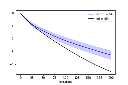
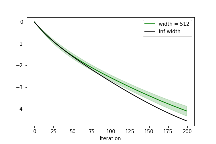
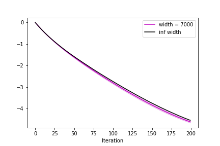
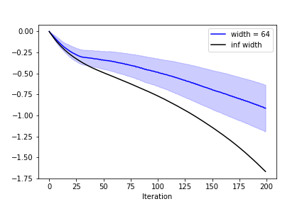
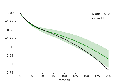
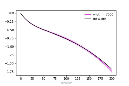
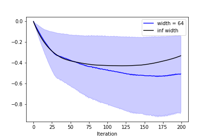
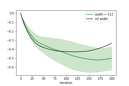
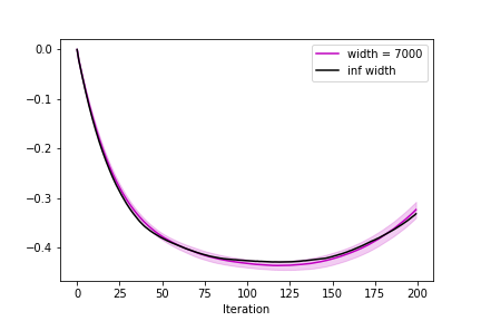
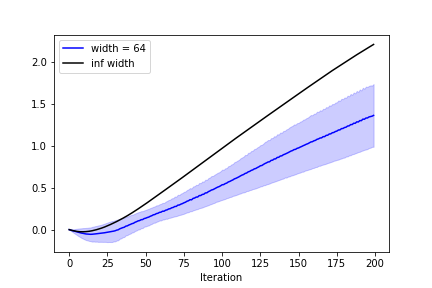
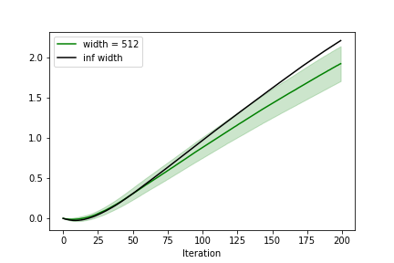
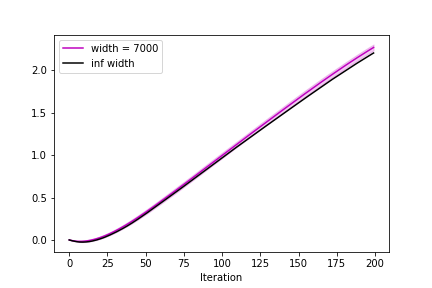
(a)	(b)	(c)

Figure 5.1: Adam training dynamics of finite and infinite-width networks in NTP. We train networks of widths 64 (a), 512 (b), 7000 (c), and track the outputs for 4 random inputs (one per row) at each iteration as the network trains. We compute the output distribution over 10 independent runs for each network, and compare with the infinite-width dynamics (black curve). As the width grows, the network function converges to that of the infinite-width dynamics captured in 2.4.9.

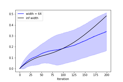
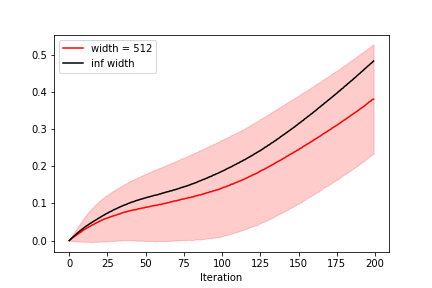
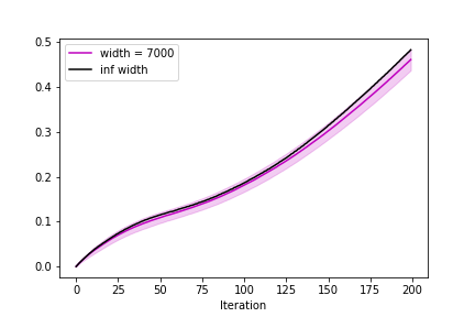
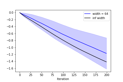
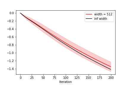
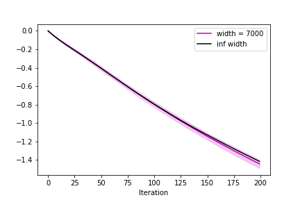
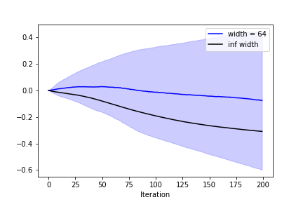
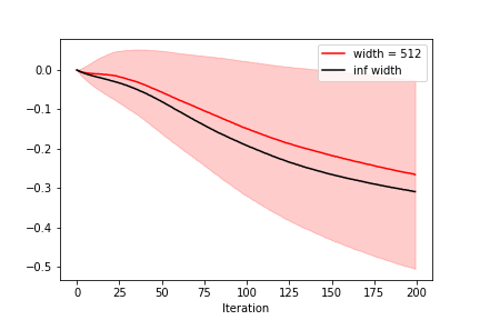
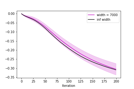
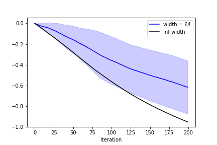
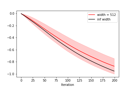
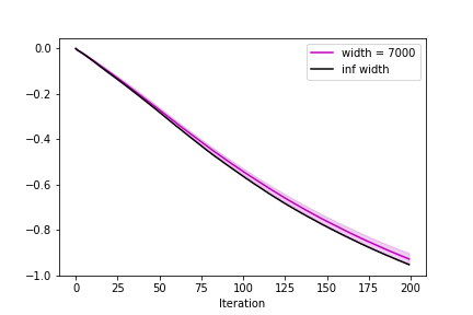
(a)	(b)	(c)

Figure 5.2: Adam training dynamics of finite and infinite-width networks in $\mu$P. We train networks of widths 64 (a), 512 (b), 7000 (c), and track the outputs for 4 random inputs (one per row) at each iteration as the network trains. We compute the output distribution over 10 independent runs for each network, and compare with the infinite-width dynamics (black curve). As the width grows, the network function converges to that of the infinite-width dynamics captured in 2.7.3.

Acknowledgements

In alphabetical order, we would like to thank Jeremy Bernstein, Nikhil Ghosh, Dror Ironi, Ariel Landau, Sadhika Malladi, Jamie Simon, and Josh Susskind for providing insightful comments and discussion.

References

- Alemohammad et al. [2021] Sina Alemohammad, Zichao Wang, Randall Balestriero, and Richard Baraniuk. The recurrent neural tangent kernel. ArXiv, abs/2006.10246, 2021.
- Allen-Zhu et al. [2019] Zeyuan Allen-Zhu, Yuanzhi Li, and Zhao Song. A convergence theory for deep learning via over-parameterization. ArXiv, abs/1811.03962, 2019.
- Arora et al. [2019] Sanjeev Arora, S. Du, Wei Hu, Zhiyuan Li, R. Salakhutdinov, and Ruosong Wang. On exact computation with an infinitely wide neural net. In NeurIPS, 2019.
- Bernstein et al. [2018] Jeremy Bernstein, Yu-Xiang Wang, Kamyar Azizzadenesheli, and Anima Anandkumar. signSGD: Compressed Optimisation for Non-Convex Problems, February 2018. URL https://arxiv.org/abs/1802.04434v3.
- Bernstein et al. [2021] Jeremy Bernstein, Arash Vahdat, Yisong Yue, and Ming-Yu Liu. On the distance between two neural networks and the stability of learning. arXiv:2002.03432 [cs, math, stat], January 2021. URL http://arxiv.org/abs/2002.03432.
- Carbonnelle & De Vleeschouwer [2019] Simon Carbonnelle and Christophe De Vleeschouwer. Layer rotation: a surprisingly powerful indicator of generalization in deep networks? arXiv:1806.01603 [cs, stat], July 2019. URL http://arxiv.org/abs/1806.01603.
- Chizat & Bach [2018] Lénaïc Chizat and Francis R. Bach. On the global convergence of gradient descent for over-parameterized models using optimal transport. In NeurIPS, 2018.
- Chizat et al. [2019] Lénaïc Chizat, Edouard Oyallon, and Francis R. Bach. On lazy training in differentiable programming. In NeurIPS, 2019.
- Dozat [2016] Timothy Dozat. Incorporating nesterov momentum into adam. 2016.
- Du et al. [2019] Simon Shaolei Du, Kangcheng Hou, Barnabás Póczos, Ruslan Salakhutdinov, Ruosong Wang, and Keyulu Xu. Graph neural tangent kernel: Fusing graph neural networks with graph kernels. ArXiv, abs/1905.13192, 2019.
- Duchi et al. [2010] John C. Duchi, Elad Hazan, and Yoram Singer. Adaptive subgradient methods for online learning and stochastic optimization. In J. Mach. Learn. Res., 2010.
- Golikov & Yang [2022] Eugene Golikov and Greg Yang. Non-Gaussian Tensor Programs. October 2022. URL https://openreview.net/forum?id=AcHUIG2wA8-.
- Hanin & Nica [2020] Boris Hanin and Mihai Nica. Finite depth and width corrections to the neural tangent kernel. ArXiv, abs/1909.05989, 2020.
- Hinton & Neal [1995] Geoffrey E. Hinton and R. Neal. Bayesian learning for neural networks. 1995.
- Hron et al. [2020] Jiri Hron, Yasaman Bahri, Jascha Narain Sohl-Dickstein, and Roman Novak. Infinite attention: Nngp and ntk for deep attention networks. In ICML, 2020.
- Huang & Yau [2020] Jiaoyang Huang and H. T. Yau. Dynamics of deep neural networks and neural tangent hierarchy. ArXiv, abs/1909.08156, 2020.
- Huang et al. [2020] Xiaoshan Huang, Felipe Pérez, Jimmy Ba, and Maksims Volkovs. Improving transformer optimization through better initialization. In ICML, 2020.
- Jacot et al. [2018] Arthur Jacot, Franck Gabriel, and Clément Hongler. Neural tangent kernel: convergence and generalization in neural networks (invited paper). Proceedings of the 53rd Annual ACM SIGACT Symposium on Theory of Computing, 2018.
- Kingma & Ba [2015] Diederik P. Kingma and Jimmy Ba. Adam: A method for stochastic optimization. CoRR, abs/1412.6980, 2015.
- Lee et al. [2018] Jaehoon Lee, Y. Bahri, Roman Novak, S. Schoenholz, Jeffrey Pennington, and Jascha Sohl-Dickstein. Deep neural networks as gaussian processes. ArXiv, abs/1711.00165, 2018.
- Lee et al. [2019] Jaehoon Lee, Lechao Xiao, Samuel S. Schoenholz, Yasaman Bahri, Jascha Sohl-Dickstein, and Jeffrey Pennington. Wide neural networks of any depth evolve as linear models under gradient descent. ArXiv, abs/1902.06720, 2019.
- Littwin et al. [2020a] Etai Littwin, T. Galanti, and L. Wolf. On random kernels of residual architectures. arXiv: Learning, 2020a.
- Littwin et al. [2020b] Etai Littwin, Tomer Galanti, Lior Wolf, and Greg Yang. On infinite-width hypernetworks. arXiv: Learning, 2020b.
- Littwin et al. [2021] Etai Littwin, Omid Saremi, Shuangfei Zhai, Vimal Thilak, Hanlin Goh, Joshua M. Susskind, and Greg Yang. Implicit Acceleration and Feature Learning in Infinitely Wide Neural Networks with Bottlenecks, July 2021. URL http://arxiv.org/abs/2107.00364. arXiv:2107.00364 [cs].
- Liu et al. [2020] Liyuan Liu, Xiaodong Liu, Jianfeng Gao, Weizhu Chen, and Jiawei Han. Understanding the difficulty of training transformers. ArXiv, abs/2004.08249, 2020.
- Liu et al. [2021] Yang Liu, Jeremy Bernstein, Markus Meister, and Yisong Yue. Learning by Turning: Neural Architecture Aware Optimisation. arXiv:2102.07227 [cs], September 2021. URL http://arxiv.org/abs/2102.07227.
- Loshchilov & Hutter [2017] Ilya Loshchilov and Frank Hutter. Decoupled weight decay regularization. In International Conference on Learning Representations, 2017.
- Malladi et al. [2022] Sadhika Malladi, Alexander Wettig, Dingli Yu, Danqi Chen, and Sanjeev Arora. A Kernel-Based View of Language Model Fine-Tuning, October 2022. URL https://arxiv.org/abs/2210.05643v3.
- Matthews et al. [2018] A. Matthews, M. Rowland, J. Hron, R. Turner, and Zoubin Ghahramani. Gaussian process behaviour in wide deep neural networks. ArXiv, abs/1804.11271, 2018.
- Mei et al. [2018a] Song Mei, Andrea Montanari, and Phan-Minh Nguyen. A mean field view of the landscape of two-layer neural networks. Proceedings of the National Academy of Sciences of the United States of America, 115:E7665 – E7671, 2018a.
- Mei et al. [2018b] Song Mei, Andrea Montanari, and Phan-Minh Nguyen. A mean field view of the landscape of two-layer neural networks. Proceedings of the National Academy of Sciences of the United States of America, 115:E7665 – E7671, 2018b.
- Nguyen & Pham [2020] Phan-Minh Nguyen and Huy-Tuan Pham. A rigorous framework for the mean field limit of multilayer neural networks. ArXiv, abs/2001.11443, 2020.
- Novak et al. [2019] Roman Novak, L. Xiao, Y. Bahri, Jaehoon Lee, Greg Yang, J. Hron, D. Abolafia, Jeffrey Pennington, and Jascha Sohl-Dickstein. Bayesian deep convolutional networks with many channels are gaussian processes. In ICLR, 2019.
- Rotskoff & Vanden-Eijnden [2018] Grant M. Rotskoff and Eric Vanden-Eijnden. Neural networks as interacting particle systems: Asymptotic convexity of the loss landscape and universal scaling of the approximation error. ArXiv, abs/1805.00915, 2018.
- Shazeer & Stern [2018] Noam Shazeer and Mitchell Stern. Adafactor: Adaptive Learning Rates with Sublinear Memory Cost. April 2018. URL https://arxiv.org/abs/1804.04235v1.
- Sirignano & Spiliopoulos [2020] Justin A. Sirignano and Konstantinos Spiliopoulos. Mean field analysis of neural networks: A law of large numbers. SIAM J. Appl. Math., 80:725–752, 2020.
- Talagrand [2014] Michel Talagrand. Upper and lower bounds for stochastic processes: modern methods and classical problems. Number 3. Folge, volume 60 in Ergebnisse der Mathematik und ihrer Grenzgebiete : a series of modern surveys in mathematics. Springer, Heidelberg ; New York, 2014. ISBN 978-3-642-54074-5. OCLC: ocn873529598.
- Tao [2012] Terence Tao. Topics in random matrix theory. Graduate studies in Mathematics, 132, 2012.
- Vaswani et al. [2017] Ashish Vaswani, Noam Shazeer, Niki Parmar, Jakob Uszkoreit, Llion Jones, Aidan N. Gomez, L. Kaiser, and Illia Polosukhin. Attention is all you need. ArXiv, abs/1706.03762, 2017.
- Yaida [2022] Sho Yaida. Meta-Principled Family of Hyperparameter Scaling Strategies. Technical Report arXiv:2210.04909, arXiv, October 2022. URL http://arxiv.org/abs/2210.04909. arXiv:2210.04909 [hep-th, stat] type: article.
- Yang [2019a] Greg Yang. Tensor programs i: Wide feedforward or recurrent neural networks of any architecture are gaussian processes. ArXiv, abs/1910.12478, 2019a.
- Yang [2019b] Greg Yang. Scaling Limits of Wide Neural Networks with Weight Sharing: Gaussian Process Behavior, Gradient Independence, and Neural Tangent Kernel Derivation. arXiv:1902.04760 [cond-mat, physics:math-ph, stat], February 2019b.
- Yang [2020a] Greg Yang. Tensor programs ii: Neural tangent kernel for any architecture. ArXiv, abs/2006.14548, 2020a.
- Yang [2020b] Greg Yang. Tensor programs iii: Neural matrix laws. ArXiv, abs/2009.10685, 2020b.
- Yang & Hu [2020] Greg Yang and Edward J. Hu. Feature learning in infinite-width neural networks. ArXiv, abs/2011.14522, 2020.
- Yang & Littwin [2021] Greg Yang and Etai Littwin. Tensor programs iib: Architectural universality of neural tangent kernel training dynamics. ArXiv, abs/2105.03703, 2021.
- Yang et al. [2022] Greg Yang, Edward J. Hu, Igor Babuschkin, Szymon Sidor, Xiaodong Liu, David Farhi, Nick Ryder, Jakub Pachocki, Weizhu Chen, and Jianfeng Gao. Tensor Programs V: Tuning Large Neural Networks via Zero-Shot Hyperparameter Transfer. arXiv:2203.03466 [cond-mat], March 2022. URL http://arxiv.org/abs/2203.03466. arXiv: 2203.03466.
- Yin et al. [1988] Y. Q. Yin, Z. D. Bai, and P. R. Krishnaiah. On the limit of the largest eigenvalue of the large dimensional sample covariance matrix. Probability Theory and Related Fields, 78(4):509–521, August 1988. ISSN 0178-8051, 1432-2064. doi: 10.1007/BF00353874. URL https://link.springer.com/10.1007/BF00353874.
- You et al. [2017] Yang You, Igor Gitman, and Boris Ginsburg. Large Batch Training of Convolutional Networks. arXiv:1708.03888 [cs], September 2017. URL http://arxiv.org/abs/1708.03888.
- You et al. [2020] Yang You, Jing Li, Sashank Reddi, Jonathan Hseu, Sanjiv Kumar, Srinadh Bhojanapalli, Xiaodan Song, James Demmel, Kurt Keutzer, and Cho-Jui Hsieh. Large Batch Optimization for Deep Learning: Training BERT in 76 minutes. arXiv:1904.00962 [cs, stat], January 2020. URL http://arxiv.org/abs/1904.00962.
- Zhang et al. [2019] J. Zhang, Sai Praneeth Karimireddy, Andreas Veit, Seungyeon Kim, Sashank J. Reddi, Surinder Kumar, and Suvrit Sra. Why adam beats sgd for attention models. ArXiv, abs/1912.03194, 2019.
- Zhou et al. [2018] Zhiming Zhou, Qingru Zhang, Guansong Lu, Hongwei Wang, Weinan Zhang, and Yong Yu. Adaptive learning rate methods. 2018.