An optimisation–based domain–decomposition reduced order model for parameter-dependent non–stationary fluid dynamics problems

Abstract

In this work, we address parametric non–stationary fluid dynamics problems within a model order reduction setting based on domain decomposition. Starting from the domain decomposition approach, we derive an optimal control problem, for which we present the convergence analysis. The snapshots for the high–fidelity model are obtained with the Finite Element discretisation, and the model order reduction is then proposed both in terms of time and physical parameters, with a standard POD–Galerkin projection. We test the proposed methodology on two fluid dynamics benchmarks: the non–stationary backward–facing step and lid–driven cavity flow. Finally, also in view of future works, we compare the intrusive POD–Galerkin approach with a non–intrusive approach based on Neural Networks.

1 Introduction

With the increase in the potential of high–performance computing in the last years, there is an immense necessity for numerical methods and approximation techniques that can perform real–time simulations of Partial Differential Equation (PDEs). The applications vary from naval, aeronautical and biomedical engineering, to name a few. There exist many techniques in order to achieve such a goal, among which reduced–order modelling [26] and domain–decomposition (DD) methods [43].

The DD methodology is a very efficient tool in the framework of PDEs. Any DD algorithm is constructed by an effective splitting of the domain of interest into different subdomains (overlapping or not), and the original problem is then restricted to each of these subdomains with some coupling conditions on the intersections of the subdomains. The coupling conditions may be very different, they depend on the physical meaning of the problem at hand, and they must render a certain degree of continuity among these subdomains (see, for example, [42, 43]). These methods are extremely important for multi–physics problems when efficient subcomponent numerical codes are already available, or when we do not have direct access to the numerical algorithms for some parts of the systems; see, for instance, [15, 19, 29, 31, 32, 33].

Model–order reduction methods are another set of methods mentioned before, which are extremely useful when dealing with real–time simulations or multi–query tasks. These methods are successfully employed in the settings of non–stationary and/or parameter–dependent PDEs. Reduced–order models (ROMs) are extremely effective thanks to the splitting of the computational effort into two stages: the offline stage, which contains the most expensive part of the computations, and the online stage, which allows performing fast computational queries using structures that are pre–computed in the offline stage; for more details, we refer to [26]. ROMs have been successfully applied in different fields such as fluid dynamics [4, 12, 13, 14, 34, 46, 49, 50, 52, 54, 55, 57], structural mechanics [8, 9, 24, 47, 56, 58] and fluid–structure interaction problems [5, 8, 37, 36]. Lately, there have also been great advances in reduced–order modelling for optimal–control problems, [40, 51, 53].

This paper is a direct extension of the work that has been carried out in the case of the stationary parameter–dependent fluid dynamics problems [41]. Here we exploit both aforementioned techniques, namely domain–decomposition methods using an optimisation approach to ensure the coupling of the interface conditions between subdomains, as it is presented, for example, in [23, 20], and we build a ROM on top of that using both intrusive [26, 50] and non–intrusive [27, 45, 38, 39, 48] approaches.

This work is structured as follows. In Section 2, we introduce the monolithic fluid dynamics problem and its time–discretisation scheme with the further derivation of the optimisation–based domain–decomposition formulation at each time step in both strong and weak forms. In Section 3, we derive a priori estimates for the solutions to Navier–Stokes equations which are then used to prove the existence and uniqueness of the minimiser to the optimal–control problem derived in the previous section. Furthermore, in Section 4 we derive the optimality condition for the resulting optimal control problem and the expression for the gradient of the objective functional with the following listing of the gradient–based optimisation algorithm. Section 5 contains the Finite Element discretisation of the problem of interest and the corresponding finite–dimensional high–fidelity optimisation problem. Section 6 deals with two ROM techniques: an intrusive Galerkin projection and a neural network (NN) algorithm, both based on a Proper Orthogonal Decomposition (POD) methodology. In Section 7, we show some numerical results for two toy problems: the backward–facing step and the lid–driven cavity flows. Conclusions will follow in Section 8.

2 Problem formulation

In this section, starting with a monolithic formulation of the time–dependent incompressible Navier–Stokes equations, we first introduce a time discretisation on the continuous level employing the implicit Euler time–stepping scheme. Then, we will describe a two–domain optimisation-based domain–decomposition formulation at each time step, and its variational formulation in the end. Here and in the next few sections, the analysis is valid for any value of the physical parameter, so for the sake of simplicity, we postpone mentioning the parameter dependence of the problem until Section 6.

2.1 Monolithic formulation

Let $\Omega$ be a physical domain of interest: we assume $\Omega$ to be an open subset of $\mathbb{R}^{2}$ and $\Gamma$ to be the boundary of $\Omega$. We also consider a finite time interval $[0,T]$ with $T>0$. Let $f:\Omega\times[0,T]\rightarrow\mathbb{R}^{2}$ be the forcing term, $\nu$ the kinematic viscosity, $u_{D}$ a given Dirichlet datum and $u_{0}$ a given initial condition. The problem reads as follows: find the velocity field $u:\Omega\times[0,T]\rightarrow\mathbb{R}^{2}$ and the pressure $p:\Omega\times[0,T]\rightarrow\mathbb{R}$ s.t.

$$\frac{\partial u}{\partial t}-\nu\Delta u+\left(u\cdot\nabla\right)u+\nabla p=f \Omega\times(0,T],$$ in (1a)

$$-\text{div}u=0 \Omega\times(0,T],$$ in (1b)

$$u=u_{D} \Gamma_{D}\times[0,T],$$ on (1c)

$$\nu\frac{\partial u}{\partial\textbf{n}}-p\textbf{n}=0 \Gamma_{N}\times[0,T],$$ on (1d)

$$u(t=0)=u_{0} \Omega,$$ in (1e)

where $\Gamma_{D}$ and $\Gamma_{N}$ are disjoint subsets of $\Gamma$ (as it is shown in Figure 1(a)) and n is an outward unit normal vector to $\Gamma_{N}$.

(a) Physical domain

(b) Domain Decomposition

Figure 1: Domain and boundaries

2.2 Time discretisation

We will start with time discretisation of problem (1). Let $\Delta t>0$, we assume the following time interval partition: $0=t_{0}<t_{1}<....<t_{M}=T$, where $t_{n}=n\Delta t$ for $n=0,...,M$. We employ the implicit Euler scheme for the incompressible Navier–Stokes equation which reads as follows: for $n\geq 1$ find $u^{n}:\Omega\rightarrow\mathbb{R}^{2}$, $p^{n}:\Omega\rightarrow\mathbb{R}$ s.t.

$$\frac{u^{n}-u^{n-1}}{\Delta t}-\nu\Delta u^{n}+\left(u^{n}\cdot\nabla\right)u^{n}+\nabla p^{n}=f^{n} \Omega,$$ in (2a)

$$-\text{div}u^{n}=0 \Omega,$$ in (2b)

$$u^{n}=u_{D}^{n} \Gamma_{D},$$ on (2c)

$$\nu\frac{\partial u^{n}}{\partial\textbf{n}}-p^{n}\textbf{n}=0 \Gamma_{N},$$ on (2d)

and for $$n=0$$

$$u^{0}=u_{0}\quad\text{in}\quad\Omega.$$ (2e)

Here we adopted the following notations: $f^{n}(\cdot)=f(\cdot,t_{n})$ and $u^{n}_{D}(\cdot)=u_{D}(\cdot,t_{n})$.

2.3 Domain Decomposition (DD) formulation

Let $\Omega_{i},\ i=1,2$, be open subsets of $\Omega$, such that $\overline{\Omega}=\overline{\Omega_{1}\cup\Omega_{2}}$,   $\Omega_{1}\cap\Omega_{2}=\emptyset$. Denote $\Gamma_{i}:=\partial\Omega_{i}\cap\Gamma,\ i=1,2,$ and $\Gamma_{0}:=\overline{\Omega_{1}}\cap\overline{\Omega_{2}}$. In the same way, we define the corresponding boundary subsets $\Gamma_{i,D}$ and $\Gamma_{i,N}$, $i=1,2$, see Figure 1(b).
The DD formulation reads as follows: for $n\geq 1$ and $i=1,2$, given $f_{i}:\Omega_{i}\times[0,T]\rightarrow\mathbb{R}^{2}$ and $u_{i,D}:\Gamma_{i,D}\times[0,T]\rightarrow\mathbb{R}^{2}$, find $u_{i}^{n}:\Omega_{i}\rightarrow\mathbb{R}^{2}$ and $p_{i}^{n}:\Omega_{i}\rightarrow\mathbb{R}$ s.t.

$$\frac{u_{i}^{n}-u_{i}^{n-1}}{\Delta t}-\nu\Delta u_{i}^{n}+\left(u_{i}^{n}\cdot\nabla\right)u_{i}^{n}+\nabla p_{i}^{n}=f_{i}^{n} \Omega_{i},$$ in (3a)

$$-\text{div}u_{i}^{n}=0 \Omega_{i},$$ in (3b)

$$u_{i}^{n}=u_{i,D}^{n} \Gamma_{i,D},$$ on (3c)

$$\nu\frac{\partial u_{i}^{n}}{\partial\textbf{n}}-p_{i}^{n}\textbf{n}=0 \Gamma_{i,N},$$ on (3d)

$$\nu\frac{\partial u_{i}^{n}}{\partial\textbf{n}_{i}}-p_{i}^{n}\textbf{n}_{i}=(-1)^{i+1}g \Gamma_{0},$$ on (3e)

for some $$g:\Gamma_{0}\rightarrow\mathbb{R}^{2} \textbf{n}_{i} \Omega_{i}$$, where by we denote an outward unit normal vector with respect to the domain and

$$u^{0}_{i}=u_{0}\quad\text{in}\quad\Omega_{i},$$ (3f)

for $$n=0$$.

For a given $g$, the solution to problem (3) might not be the same as the solution to problem (2), that is $u_{1}^{n}\neq u^{n}|_{\Omega_{1}}$, $p_{1}^{n}\neq p^{n}|_{\Omega_{1}}$, $u_{2}^{n}\neq u^{n}|_{\Omega_{2}}$ and $p_{2}^{n}\neq p^{n}|_{\Omega_{2}}$. On the other hand, there exists a choice for $g$, $g=\left(\nu\frac{\partial u^{n}_{1}}{\partial\textbf{n}_{1}}-p_{1}^{n}\textbf{n}_{1}\right)|_{\Gamma_{0}}=-\left(\nu\frac{\partial u^{n}_{2}}{\partial\textbf{n}_{2}}-p_{2}^{n}\textbf{n}_{2}\right)|_{\Gamma_{0}}$, such that the solution to (3) coincides with the solution to (2) on the corresponding subdomains. Therefore, we must find such a $g$, so that $u_{1}^{n}$ is as close as possible to $u_{2}^{n}$ at the interface $\Gamma_{0}$. One way to accomplish this is to minimise the functional

$$\mathcal{J}(u_{1}^{n},u_{2}^{n}):=\frac{1}{2}\int_{\Gamma_{0}}\left|u_{1}^{n}-u_{2}^{n}\right|^{2}d\Gamma.$$ (4)

Instead of (4), we can also consider the penalised or regularised functional

$$\mathcal{J}_{\gamma}(u_{1}^{n},u_{2}^{n};g):=\frac{1}{2}\int_{\Gamma_{0}}\left|u_{1}^{n}-u_{2}^{n}\right|^{2}d\Gamma+\frac{\gamma}{2}\int_{\Gamma_{0}}\left|g\right|^{2}d\Gamma,$$ (5)

where $\gamma$ is a constant that can be chosen to change the relative importance of the terms in (5). Thus, we face an optimisation problem under PDE constraints: minimise the functional (4) (or (5)) over a suitable function $g$, subject to (3).

2.4 Variational Formulation of the PDE constraints

For $i=1,2$ define the following spaces:

• $V_{i}:=\left\{u\in H^{1}(\Omega_{i};\mathbb{R}^{2})\right\}$,

• $V_{i,0}:=\left\{u\in H^{1}(\Omega_{i};\mathbb{R}^{2}):\ u|_{\Gamma_{i,D}}=0\right\}$,

• $Q_{i}:=\left\{p\in L^{2}(\Omega_{i};\mathbb{R})\right\}$.

The spaces $V_{i}$ are endowed with the $H^{1}(\Omega_{i})$–norm for $i=1,2$, the spaces $V_{i,0}$ with the $H_{0}^{1}(\Omega_{i})$–norm and the spaces $Q_{i}$ with the $L^{2}(\Omega_{i})$–norm for $i=1,2$.

Then, we define the following bilinear and trilinear forms: for i=1,2

• $m_{i}:V_{i}\times V_{i,0}\rightarrow\mathbb{R},\quad m_{i}(u_{i},v_{i}):=(u_{i},v_{i})_{\Omega_{i}}$,

• $a_{i}:V_{i}\times V_{i,0}\rightarrow\mathbb{R},\quad a_{i}(u_{i},v_{i}):=\nu(\nabla u_{i},\nabla v_{i})_{\Omega_{i}}$,

• $b_{i}:V_{i}\times Q_{i}\rightarrow\mathbb{R},\quad b_{i}(v_{i},q_{i}):=-(\text{div}v_{i},q_{i})_{\Omega_{i}}$,

• $c_{i}:V_{i}\times V_{i}\times V_{i,0}\rightarrow\mathbb{R},\quad c_{i}(u_{i},w_{i},v_{i}):=\left((u_{i}\cdot\nabla)w_{i},v_{i}\right)_{\Omega_{i}}$,

where $(\cdot,\cdot)_{\omega}$ indicates the $L^{2}(\omega)$ inner product.

Consequently, the variational counterpart of (3) reads as follows: for $n\geq 1$ and $i=1,2$, find $u_{i}\in V_{i}$ and $p_{i}\in Q_{i}$ s.t.

$$\begin{split}\frac{1}{\Delta t}m_{i}\left(u_{i}^{n}-u_{i}^{n-1},v_{i}\right)+&a_{i}(u_{i}^{n},v_{i})+c_{i}(u_{i}^{n},u_{i}^{n},v_{i})+b_{i}(v_{i},p_{i}^{n})\\ &\quad=(f_{i}^{n},v_{i})_{\Omega_{i}}+\left((-1)^{i+1}g,v_{i}\right)_{\Gamma_{0}}\quad\forall v_{i}\in V_{i,0},\end{split}$$ (6a)

$$b_{i}(u_{i}^{n},q_{i})=0\quad\quad\forall q_{i}\in Q_{i},$$ (6b)

$$\quad\quad u_{i}^{n}=u_{i,D}^{n}\quad\quad\text{on}\ \Gamma_{i,D}.$$ (6c)

3 Analysis of the optimal control problem

In this section, we would like to give an overview of the existence of local minima of the optimal–control problem described above. It will rely on the a priori estimates for the solutions to the Navier–Stokes equations. Due to the presence of the Neumann boundary condition, the analysis of the state problem is not possible, so we will modify the problem in the framework where the problem is well posed and give some indication about the original problem later in the section.

3.1 A modified Navier–Stokes problem

First, without loss of generality, we assume that the Dirichlet data $u_{i,D}$ is homogeneous. Otherwise, we can use various techniques, e.g., lifting functions as will be discussed later on, to obtain a problem with homogeneous Dirichlet boundary conditions on $\Gamma_{i,D}$. As mentioned in the preface to this section, it is hard to prove the well–posedness of the solution to the Navier–Stokes equation in the form (6). The main problem arises from the nonlinear term $c_{i}(u_{i}^{n},u_{i}^{n},v_{i})=\left((u_{i}^{n}\cdot\nabla)u_{i}^{n},v_{i}\right)_{\Omega_{i}^{n}}$. Indeed, by integration by parts and the incompressibility conditions (6b), we can see

$$c_{i}(u_{i}^{n},u_{i}^{n},v_{i}) =\int_{\Omega_{i}}(u_{i}^{n}\cdot\nabla)u_{i}^{n}\cdot v_{i}d\Omega=\int_{\partial\Omega_{i}}(u_{i}^{n}\cdot v_{i})(u_{i}^{n}\cdot\textbf{n})d\Gamma$$

$$-\int_{\Omega_{i}}(u_{i}^{n}\cdot v_{i})\,\text{div}\,u_{i}^{n}d\Omega-\int_{\Omega_{i}}(u_{i}^{n}\cdot\nabla)v_{i}\cdot u_{i}^{n}d\Omega$$

$$=\int_{\partial\Omega_{i}}(u_{i}^{n}\cdot v_{i})(u_{i}^{n}\cdot\textbf{n})d\Gamma-\int_{\Omega_{i}}(u_{i}^{n}\cdot\nabla)v_{i}\cdot u_{i}^{n}d\Omega$$

$$=\int_{\Gamma_{i,N}\cup\Gamma_{0}}(u_{i}^{n}\cdot v_{i})(u_{i}^{n}\cdot\textbf{n})d\Gamma-c_{i}(u_{i}^{n},v_{i},u_{i}^{n}),$$

which leads to the following expression

$$c_{i}(u_{i}^{n},u_{i}^{n},u_{i}^{n})=\frac{1}{2}\int_{\Gamma_{i,N}\cup\Gamma_{0}}|u_{i}^{n}|^{2}(u_{i}^{n}\cdot\textbf{n})d\Gamma.$$ (7)

As we can see, the problem here is due to the fact that this boundary term has an unknown sign, which complicates further analysis. On the other hand, it gives us an idea of how to redefine the problem at hand in order to obtain well–posedness (see, e.g. [10]). We rewrite the Neumann–type outlet conditions and the coupling stress conditions between subdomains in the following way:

$$\nu\frac{\partial u_{i}^{n}}{\partial\textbf{n}}-p_{i}^{n}\textbf{n}-\frac{1}{2}(u_{i}^{n}\cdot\textbf{n})u_{i}^{n}=0 \Gamma_{i,N},$$ on (8)

$$\nu\frac{\partial u_{i}^{n}}{\partial\textbf{n}_{i}}-p_{i}^{n}\textbf{n}_{i}-\frac{1}{2}(u_{i}^{n}\cdot\textbf{n}_{i})u_{i}^{n}=(-1)^{i+1}g \Gamma_{0}.$$ on (9)

This, in turn, leads to a new variational formulation of the state equations (3): for $n\geq 1$ and $i=1,2$, find $u_{i}^{n}\in V_{i,0}$ and $p_{i}^{n}\in Q_{i}$ s.t.

$$\begin{split}\frac{1}{\Delta t}m_{i}\left(u_{i}^{n}-u_{i}^{n-1},v_{i}\right)+&a_{i}(u_{i}^{n},v_{i})+\tilde{c}_{i}(u_{i}^{n},u_{i}^{n},v_{i})+b_{i}(v_{i},p_{i}^{n})\\ &\quad=(f_{i}^{n},v_{i})_{\Omega_{i}}+\left((-1)^{i+1}g,v_{i}\right)_{\Gamma_{0}}\quad\quad\forall v_{i}\in V_{i,0},\end{split}$$ (10a)

$$b_{i}(u_{i}^{n},q_{i})=0\quad\quad\forall q_{i}\in Q_{i},$$ (10b)

where the trilinear form $\tilde{c}(\cdot,\cdot,\cdot)$ is defined as

$$\tilde{c}_{i}(u_{i},w_{i},v_{i})=\frac{1}{2}\left((u_{i}\cdot\nabla)w_{i},v_{i}\right)_{\Omega_{i}}-\frac{1}{2}\left((u_{i}\cdot\nabla)v_{i},w_{i}\right)_{\Omega_{i}}$$ (11)

and it has the following remarkable property

$$\tilde{c}_{i}(u_{i},v_{i},v_{i})=0\quad\forall u_{i},v_{i}\in V_{i,0}.$$ (12)

3.2 A priori estimates

We now first introduce the various well–known properties of the different terms entering the weak formulation (10), i.e.

• the forms $m_{i}(\cdot.\cdot)$, $a_{i}(\cdot,\cdot)$ and $\tilde{c}_{i}(\cdot,\cdot,\cdot)$ are continuous: there exist positive constants $C_{m}$, $C_{a}$ and $C_{c}$ such that

  $$|m_{i}(u_{i},v_{i})|\leq C_{m}||u_{i}||_{V_{i,0}}||v_{i}||_{V_{i,0}}\quad \forall u_{i},v_{i}\in V_{i,0},$$ (13)

  $$|a_{i}(u_{i},v_{i})|\leq C_{a}||u_{i}||_{V_{i,0}}||v_{i}||_{V_{i,0}}\quad \forall u_{i},v_{i}\in V_{i,0},$$ (14)

  $$|\tilde{c}_{i}(u_{i},w_{i},v_{i})|\leq C_{c}||u_{i}||_{V_{i,0}}||w_{i}||_{V_{i,0}}||v_{i}||_{V_{i,0}}\quad \forall u_{i},w_{i},v_{i}\in V_{i,0},$$ (15)

• the bilinear form $a_{i}(\cdot,\cdot)$ is coercive: there exists a positive constant $\alpha>0$ such that

  $$a_{i}(v_{i},v_{i})\geq\alpha||v_{i}||_{V_{i,0}}^{2}\quad\forall v_{i}\in V_{i,0},$$ (16)

• the bilinear form $b_{i}(\cdot,\cdot)$ satisfies inf–sup condition: there exists a positive constant $\beta>0$ such that

  $$\sup\limits_{v_{i}\in V_{i,0}\backslash\{0\}}\frac{b_{i}(v_{i},q_{i})}{||v_{i}||_{V_{i,0}}}\geq\beta||q_{i}||_{Q_{i}}\quad\forall q_{i}\in Q_{i},$$ (17)

• the bilinear form $m_{i}(\cdot,\cdot)$ is non–negative definite, i.e.

  $$m_{i}(v_{i},v_{i})=||v_{i}||_{L^{2}(\Omega_{i})}^{2}\geq 0\quad\forall v_{i}\in V_{i,0}.$$ (18)

  By using the properties (13) (16), (12), (18), the trace theorem and equations (10), we are able to write the following estimate for the solution $u_{i}^{n}$ and $p_{i}^{n}$ to (10)

  $$||u_{i}^{n}||_{V_{i,0}}^{2} \leq \frac{1}{\alpha}a_{i}(u_{i}^{n},u_{i}^{n})\leq\frac{1}{\alpha}a_{i}(u_{i}^{n},u_{i}^{n})+\frac{1}{\alpha\Delta t}m_{i}(u_{i}^{n},u_{i}^{n})$$

  $$= \frac{1}{\alpha}\left(\frac{1}{\Delta t}m_{i}(u_{i}^{n-1},u_{i}^{n})-\tilde{c}_{i}(u_{i}^{n},u_{i}^{n},u_{i}^{n})-b_{i}(u_{i}^{n},p_{i}^{n})\right.$$

  $$+ \left.(f_{i}^{n},u_{i}^{n})_{\Omega_{i}}+(-1)^{i+1}(g,u_{i}^{n})_{\Gamma_{0}}\right)$$

  $$\leq \frac{1}{\alpha}\left(\frac{C_{m}}{\Delta t}||u_{i}^{n-1}||_{V_{i,0}}+||f_{i}^{n}||_{L^{2}(\Omega_{i})}+||g||_{L^{2}(\Gamma_{0})}\right)||u_{i}^{n}||_{V_{i,0}},$$

  which leads to the following estimate:

  $$||u_{i}^{n}||_{V_{i,0}}\leq\frac{1}{\alpha}\left(\frac{C_{m}}{\Delta t}||u_{i}^{n-1}||_{V_{i,0}}+||f_{i}^{n}||_{L^{2}(\Omega_{i})}+||g||_{L^{2}(\Gamma_{0})}\right).$$ (19)

  Similarly, by using (17), (13), (14), (15) and equations (10), we obtain

  $$||p_{i}^{n}||_{Q_{i}} \leq \frac{1}{\beta}\sup\limits_{v_{i}\in V_{i,0}\backslash\{0\}}\frac{b_{i}(v_{i},p_{i}^{n})}{||v_{i}||_{V_{i,0}}}\leq\frac{1}{\beta}\sup\limits_{v_{i}\in V_{i,0}\backslash\{0\}}\frac{\frac{1}{\Delta t}|m_{i}(u_{i}^{n}-u_{i}^{n-1},v_{i})|}{||v_{i}||_{V_{i,0}}}$$

  $$+ \frac{1}{\beta}\sup\limits_{v_{i}\in V_{i,0}\backslash\{0\}}\frac{|a_{i}(u_{i}^{n},v_{i})|+|c_{i}(u_{i}^{n},u_{i}^{n},v_{i})|+|(f_{i}^{n},v_{i})_{\Omega_{i}}|}{||v_{i}||_{V_{i,0}}}$$

  $$+ \frac{1}{\beta}\sup\limits_{v_{i}\in V_{i,0}\backslash\{0\}}\frac{|(g,v_{i})_{\Gamma_{0}}|}{||v_{i}||_{V_{i,0}}}\leq\frac{1}{\beta}\left(\frac{C_{m}}{\Delta t}+C_{a}+C_{c}||u_{i}^{n}||_{V_{i,0}}\right)||u_{i}^{n}||_{V_{i,0}}$$

  $$+ \frac{1}{\beta}\left(\frac{C_{m}}{\Delta t}||u_{i}^{n-1}||_{V_{i,0}}+||f_{i}^{n}||_{L^{2}(\Omega_{i})}+||g||_{L^{2}(\Gamma_{0})}\right),$$

  which together with the estimate (19) leads to

  $$||p_{i}^{n}||_{Q_{i}} \leq \frac{1}{\beta}\left[\left(1+\frac{1}{\alpha}\left(\frac{C_{m}}{\Delta t}+C_{a}\right)\right)\left(\frac{C_{m}}{\Delta t}||u_{i}^{n-1}||_{V_{i,0}}+||f_{i}^{n}||_{L^{2}(\Omega_{i})}\right.\right.$$

  $$+ \left.\left.||g||_{L^{2}(\Gamma_{0})}\right)+\frac{C_{c}}{\alpha^{2}}\left(\frac{C_{m}}{\Delta t}||u_{i}^{n-1}||_{V_{i,0}}+||f_{i}^{n}||_{L^{2}(\Omega_{i})}+||g||_{L^{2}(\Gamma_{0})}\right)^{2}\right].$$

3.3 Existence of optimal solutions

In this subsection, we prove the existence of optimal solutions for the regularised functional (5). The proof follows the methodology presented by Gunzburger et al. [21]. Firstly, we define the admissibility set as follows:

$$\mathcal{U}_{ad}=\left\{(u_{1}^{n},p_{1}^{n},u_{2}^{n},p_{2}^{n},g)\in V_{1,0}\times Q_{1}\times V_{2,0}\times Q_{2}\times L^{2}(\Gamma_{0})\text{ such that}\quad\quad\quad\right.$$

$$\left.\text{equations }\eqref{eq:state_new}\text{ are satisfied and }\mathcal{J}_{\gamma}(u_{1}^{n},u_{2}^{n};g)<\infty\right\}.$$

The admissibility set is clearly non–empty, since, as it was pointed out above, the restrictions to subdomains of the monolithic solution and its corresponding flux on the interface belong to the set.

Let $\left\{\left(u_{1}^{n,(j)},p_{1}^{n,(j)},u_{2}^{n,(j)},p_{2}^{n,(j)},g^{(j)}\right)\right\}$ be a minimizing sequence in $\mathcal{U}_{ad}$, i.e.,

$$\lim\limits_{j\rightarrow\infty}\mathcal{J}_{\gamma}\left(u_{1}^{n,(j)},u_{2}^{n,(j)},g^{(j)}\right)=\inf\limits_{(u_{1}^{n},p_{1}^{n},u_{2}^{n},p_{2}^{n},g)\in\mathcal{U}_{ad}}\mathcal{J}_{\gamma}(u_{1}^{n},u_{2}^{n},g).$$

From the definition of the admissible set $\mathcal{U}_{ad}$ and the functional $\mathcal{J}_{\gamma}$, it is evident that the set $\left\{g^{(j)}\right\}$ is uniformly bounded in $L^{2}(\Gamma_{0})$, which in turn, due to the a priori estimates (19) and (• ‣ 3.2), implies that the sets $\left\{\left(u_{i}^{n,(j)}\right)\right\}$ are uniformly bounded in $V_{i,0}$ and the sets $\left\{\left(p_{i}^{n,(j)}\right)\right\}$ are uniformly bounded in $Q_{i}$ for $i=1,2$. Thus there exists a point $\left(\hat{u}_{1}^{n},\hat{p}_{1}^{n},\hat{u}_{2}^{n},\hat{p}_{2}^{n},\hat{g}\right)\in\mathcal{U}_{ad}$ and a subsequence $\left\{\left(u_{1}^{n,(j_{k})},p_{1}^{n,(j_{k})},u_{2}^{n,(j_{k})},p_{2}^{n,(j_{k})},g^{(j_{k})}\right)\right\}$ of the minimising sequence such that for $i=1,2$

$$u_{i}^{n,(j_{k})}\rightharpoonup\hat{u}_{i}^{n} V_{i,0},$$ in (21)

$$p_{i}^{n,(j_{k})}\rightharpoonup\hat{p}_{i}^{n} Q_{i},$$ in (22)

$$g^{(j_{k})}\rightharpoonup\hat{g} L^{2}(\Gamma_{0}),$$ in (23)

$$u_{i}^{n,(j_{k})}\rightarrow\hat{u}_{i}^{n} L^{2}(\Omega_{i}),$$ in (24)

$$u_{i}^{n,(j_{k})}|_{\Gamma_{0}}\rightarrow\hat{u}_{i}^{n}|_{\Gamma_{0}} L^{2}(\Gamma_{0}).$$ in (25)

The last two results are obtained by the trace theorem and compact embedding results in Sobolev spaces, see for example [16, 35].

Since the forms $m_{i}(\cdot,\cdot)$, $a_{i}(\cdot,\cdot)$ and $b_{i}(\cdot,\cdot)$ are bilinear and continuous by (21), (22) and (23) we obtain the following convergence results:

$$m_{i}(u_{i}^{n,(j_{k})},v_{i})\rightarrow m_{i}(\hat{u}_{i}^{n},v_{i}) \forall v_{i}\in V_{i,0},$$

$$a_{i}(u_{i}^{n,(j_{k})},v_{i})\rightarrow a_{i}(\hat{u}_{i}^{n},v_{i}) \forall v_{i}\in V_{i,0},$$

$$b_{i}(u_{i}^{n,(j_{k})},q_{i})\rightarrow b_{i}(\hat{u}_{i}^{n},q_{i}) \forall q_{i}\in Q_{i},$$

$$b_{i}(v_{i},p_{i}^{n,(j_{k})})\rightarrow b_{i}(v_{i},\hat{p}_{i}^{n}) \forall v_{i}\in V_{i,0},$$

$$(g^{(j_{k})},v_{i})_{\Gamma_{0}}\rightarrow(\hat{g},v_{i})_{\Gamma_{0}} \forall v_{i}\in V_{i,0}.$$

Concerning the trilinear form $\tilde{c}_{i}(\cdot,\cdot,\cdot)$, we exploit integration by part twice, divergence–free conditions for $u_{i}^{n,(j_{k})}$ and $\hat{u}_{i}^{n}$, and the strong convergence results (24)–(25). We obtain $\forall v_{i}\in V_{i,0}$

$$\lim\limits_{k\rightarrow\infty}\frac{1}{2}\int_{\Omega_{i}}(u_{i}^{n,(j_{k})}\cdot\nabla)v_{i}\cdot u_{i}^{n,(j_{k})}d\Omega=\frac{1}{2}\int_{\Omega_{i}}(\hat{u}_{i}^{n}\cdot\nabla)v\cdot\hat{u}_{i}^{n}d\Omega,$$

$$\lim\limits_{k\rightarrow\infty}\frac{1}{2}\int_{\Omega_{i}}(u_{i}^{n,(j_{k})}\cdot\nabla)u_{i}^{n,(j_{k})}\cdot v_{i}d\Omega=\lim\limits_{k\rightarrow\infty}\frac{1}{2}\int_{\Gamma_{0}}\left(u_{i}^{n,(j_{k})}\cdot v_{i}\right)\left(u_{i}^{n,(j_{k})}\cdot\textbf{n}_{i}\right)d\Gamma$$

$$-\lim\limits_{k\rightarrow\infty}\frac{1}{2}\int_{\Omega_{i}}(u_{i}^{n,(j_{k})}\cdot\nabla)v_{i}\cdot u_{i}^{n,(j_{k})}d\Omega=\frac{1}{2}\int_{\Gamma_{0}}\left(\hat{u}_{i}^{n}\cdot v_{i}\right)\left(\hat{u}_{i}^{n}\cdot\textbf{n}_{i}\right)d\Gamma$$

$$-\frac{1}{2}\int_{\Omega_{i}}(\hat{u}_{i}^{n}\cdot\nabla)v_{i}\cdot\hat{u}_{i}^{n,}d\Omega=\frac{1}{2}\int_{\Omega_{i}}(\hat{u}_{i}^{n}\cdot\nabla)\hat{u}_{i}^{n}\cdot v_{i}d\Omega,$$

which leads to

$$\lim\limits_{k\rightarrow\infty}\tilde{c}_{i}(u_{i}^{n,(j_{k})},u_{i}^{n,(j_{k})},v_{i})=\tilde{c}_{i}(\hat{u}_{i}^{n},\hat{u}_{i}^{n},v_{i}) \forall v_{i}\in V_{i,0}.$$

These convergence results mean that the functions $\hat{u}_{1}^{n},\hat{p}_{1}^{n},\hat{u}_{2}^{n},\hat{p}_{2}^{n},\hat{g}$ satisfy the state equations (10). We also note that the functional $\mathcal{J}_{\gamma}$ is lower–semicontinuous, i.e

$$\liminf\limits_{j\rightarrow\infty}\mathcal{J}_{\gamma}(u_{1}^{n,(j_{k})},u_{2}^{n,(j_{k})},g^{(j_{k})})\geq\mathcal{J}_{\gamma}(\hat{u}_{1}^{n},\hat{u}_{2}^{n},\hat{g}),$$

which implies that

$$\inf\limits_{(u_{1}^{n},p_{1}^{n},u_{2}^{n},p_{2}^{n},g)\in\mathcal{U}_{ad}}\mathcal{J}_{\gamma}(u_{1}^{n},u_{2}^{n},g)=\mathcal{J}_{\gamma}(\hat{u}_{1}^{n},\hat{u}_{2}^{n},\hat{g}).$$

Hence, we have proved the existence of optimal solutions.

3.4 Convergence with vanishing penalty parameter

In the previous section, we have proved the existence of optimal solutions of the regularised function $\mathcal{J}_{\gamma}$ for any $\gamma>0$, where the parameter $\gamma$ indicates the relative importance of the two terms entering the definition of the functional. This poses an issue in our domain–decomposition setting since the optimal solution does not satisfy the coupling condition $u_{1}^{n}|_{\Gamma_{0}}=u_{2}^{n}|_{\Gamma_{0}}$. In this section, we prove the existence of an optimal solution to the unregularised functional $\mathcal{J}$ with corresponds to the functional $\mathcal{J}_{\gamma}$ with $\gamma=0$.

Let $(u^{n,mon},p^{n,mon})$ be a weak solution to the monolithic equations (2), and for each $\gamma>0$ we denote by $(u_{1}^{n,\gamma},p_{1}^{n,\gamma},u_{2}^{n,\gamma},p_{2}^{n,\gamma},g^{\gamma})$ an optimum of $\mathcal{J}_{\gamma}$ under the constraints (10). We define the following functions for $i=1,2$:

$$u_{i}^{n,mon} := u^{n,mon}|_{\Omega_{i}},$$

$$p_{i}^{n,mon} := p^{n,mon}|_{\Omega_{i}},$$

$$g^{mon} := \nu\frac{\partial u_{1}^{n,mon}}{\partial\textbf{n}_{1}}-p_{1}^{n,mon}\textbf{n}_{1}-\frac{1}{2}(u_{1}^{n,mon}\cdot\textbf{n}_{1})u_{1}^{n,mon}\quad\text{on }\Gamma_{0}.$$

Due to optimality of the point $(u_{1}^{n,\gamma},p_{1}^{n,\gamma},u_{2}^{n,\gamma},p_{2}^{n,\gamma},g^{\gamma})$, we obtain that $\forall\gamma>0$

$$\mathcal{J}_{\gamma}(u_{1}^{n,\gamma},p_{1}^{n,\gamma},u_{2}^{n,\gamma},p_{2}^{n,\gamma},g^{\gamma})\leq\mathcal{J}_{\gamma}(u_{1}^{n,mon},p_{1}^{n,mon},u_{2}^{n,mon},p_{2}^{n,mon},g^{mon}),$$

which due to the definition of $u_{1}^{n,mon}$ and $u_{2}^{n,mon}$ gives us the following bound:

$$\frac{1}{2}\int_{\Gamma_{0}}\left|u_{1}^{n,\gamma}-u_{2}^{n,\gamma}\right|^{2}d\Gamma+\frac{\gamma}{2}\int_{\Gamma_{0}}\left|g^{\gamma}\right|^{2}d\Gamma\leq\frac{\gamma}{2}\int_{\Gamma_{0}}\left|g^{mon}\right|^{2}d\Gamma\quad\forall\gamma>0.$$

The last inequality tells as that the sequence $\{g^{\gamma}:\gamma>0\}$ is bounded in $L^{2}(\Gamma_{0})$. Following the exact same lines of arguments as in the previous section, we are able to deduce that there is a subsequence of the original sequence (we will keep the same notation for the sake of simplicity) that converges to $(u_{1}^{n,\ast},p_{1}^{n,\ast},u_{2}^{n,\ast},p_{2}^{n,\ast},g^{\ast})\in V_{1,0}\times Q_{1}\times V_{2,0}\times Q_{2}\times L^{2}(\Gamma_{0})$ in the sense of (21) – (25). In addition to this, the inequality above tells us that $||u_{1}^{n,\gamma}-u_{2}^{n,\gamma}||_{L^{2}(\Gamma_{0})}\rightarrow 0$ as $\gamma\rightarrow 0$, which in turn yields $u_{1}^{1,\ast}=u_{2}^{1,\ast}$ a.e. on $\Gamma_{0}$. The non–negativity of $\mathcal{J}$ leads to the fact that $(u_{1}^{n,\ast},p_{1}^{n,\ast},u_{2}^{n,\ast},p_{2}^{n,\ast},g^{\ast})$ is a global minimum of $\mathcal{J}$. Also, it is easy to see that the following functions $u^{n,\ast}\in{H_{0,\Gamma_{D}}^{1}(\Omega)},p^{n,\ast}\in L^{2}(\Omega)$, defined as

$$u^{n,\ast}:=\begin{cases}u_{1}^{n,\ast},\quad\text{ in }\Omega_{1}\cup\Gamma_{0},\\ u_{2}^{n,\ast},\quad\text{ in }\Omega_{2}\cup\Gamma_{0},\end{cases}p^{n,\ast}:=\begin{cases}p_{1}^{n,\ast},\quad\text{ in }\Omega_{1}\cup\Gamma_{0},\\ p_{2}^{n,\ast},\quad\text{ in }\Omega_{2}\cup\Gamma_{0},\end{cases}$$

satisfy the monolithic equations (2) in the weak sense.

Remark (Uniqueness of optimal solutions).

It is well–known that the solution to the non–stationary incompressible Navier–Stokes equation in 2D is unique [44], and it can be proved that uniqueness transfers to the implicit–Euler time–discretisation scheme with a good choice of a time–step parameter (see, for instance, [25]). This, together with the convexity of the objective functional, leads to the uniqueness of the optimal solution discussed above.

Remark (Weak formulation with “non–symmetric” trilinear form).

As we pointed out the condition (12) was essential in order to conduct the analysis of the optimal–control problem. Concerning the problem posed in the weak from (6), the numerical experiments show the same convergence results as in the case where the trilinear form (11) is adopted.

4 Optimality system and optimisation algorithms

In this section, we will provide the tools to tackle the optimal–control problem that arises in Section 2.3. First, we will derive the optimality system by means of Lagrangian functional. Then, we will use the sensitivity derivatives technique to obtain the representation for the gradient of the objective functional, which will allow us to define an optimisation–based minimisation algorithm for the optimal–control problem in hand.

4.1 Optimality system

One of the ways to address the constrained optimisation problem is to reformulate the initial problem in terms of a Lagrangian functional by introducing the so–called adjoint variables. In this way, the optimal solution to the original problem is sought among the stationary points of the Lagrangian, see, for instance, [22, 28].

We define the Lagrangian functional as follows:

$$\begin{split}&\mathcal{L}(u_{1}^{n},p_{1}^{n},u_{2}^{n},p_{2}^{n},\xi_{1},\xi_{2},\lambda_{1},\lambda_{2};g):=\mathcal{J}_{\gamma}(u_{1}^{n},u_{2}^{n};g)\\ -&\sum\limits_{i=1}^{2}\left[\frac{m_{i}(u_{i}^{n}-u_{i}^{n-1},\xi_{i})}{\Delta t}+a_{i}(u_{i}^{n},\xi_{i})+c_{i}(u_{i}^{n},u_{i}^{n},\xi_{i})+b_{i}(\xi_{i},p_{i}^{n})+b_{i}(u_{i}^{n},\lambda_{i})\right]\\ +&\sum\limits_{i=1}^{2}(f_{i}^{n},\xi_{i})_{\Omega_{i}}+\sum\limits_{i=1}^{2}((-1)^{i+1}g,\xi_{i})_{\Gamma_{0}}.\end{split}$$ (26)

The Lagrangian functional above takes into account our objective functional (5) and the PDE constraints (6) multiplied by additional so–called adjoint variables $\xi_{1},\xi_{2},\lambda_{1},\lambda_{2}$ $\in V_{1,0}\times Q_{1}\times V_{2,0}\times Q_{2}$. It is proved (see, e.g. [28]) that the optimal solution to the constrained optimisation problem (5)–(6) coincides with stationary points of the higher–dimensional functional (LABEL:eq:lagrangian) that, in turn, gives us an easy way to obtain the optimality conditions.

Notice that, technically, we should also have included Lagrange multipliers corresponding to the non–homogeneous Dirichlet boundary conditions (6c) in the definition of the functional $\mathcal{L}$. However, since the functional $\mathcal{J}_{\gamma}$ (5) does not explicitly depend on $u_{1,D}^{n}$ and $u_{2,D}^{n}$, the corresponding adjoint Dirichlet boundary conditions will be homogeneous on these parts of the boundaries.

We now apply the necessary conditions for finding stationary points of $\mathcal{L}$. Setting to zero the first variations w.r.t. $\xi_{i}\in V_{i,0}$ and $\lambda_{i}\in{Q_{i}}$, for $i=1,2,$ yields the state equations (6a)–(6b). Setting to zero the first variations w.r.t. $u_{1}^{n}$, $p_{1}^{n}$, $u_{2}^{n}$ and $p_{2}^{n}$ yields the adjoint equations:

$$\begin{split}\frac{1}{\Delta t}m_{i}(\eta_{i},\xi_{i})+a_{i}(\eta_{i},\xi_{i})&+c_{i}\left(\eta_{i},u_{i}^{n},\xi_{i}\right)+c_{i}\left(u_{i}^{n},\eta_{i},\xi_{i}\right)\\ &+b_{i}(\eta_{i},\lambda_{i})=((-1)^{i+1}\eta_{i},u_{1}^{n}-u_{2}^{n})_{\Gamma_{0}},\end{split} \forall\eta_{i}\in V_{i,0},$$ (27a)

$$b_{i}(\xi_{i},\mu_{i})=0, \forall\mu_{i}\in Q_{i}.$$ (27b)

Finally, setting to zero the first variations w.r.t. $g\in L^{2}(\Gamma_{0})$ yields the optimality condition:

$$\gamma(h,g)_{\Gamma_{0}}+(h,\xi_{1}-\xi_{2})_{\Gamma_{0}}=0,\quad\forall h\in L^{2}(\Gamma_{0}).$$ (28)

4.2 Sensitivity derivatives

In order to obtain the expression for the gradient of the optimisation problem at hand, we will resort to the sensitivity approach, see for instance [22, 28]. The approach consists of finding equations for directional derivatives of the state variables with respect to the control, called sensitivities.

The first derivative $\frac{d\mathcal{J}_{\gamma}}{dg}$ of $\mathcal{J}_{\gamma}$ is defined through its action on the variation $\tilde{g}$ as follows:

$$\left<\frac{d\mathcal{J}_{\gamma}}{dg},\tilde{g}\right>=(u_{1}^{n}-u_{2}^{n},\tilde{u}_{1}-\tilde{u}_{2})_{\Gamma_{0}}+\gamma(g,\tilde{g})_{\Gamma_{0}},$$ (29)

where $\tilde{u}_{1}\in V_{1,0}$, $\tilde{u}_{2}\in V_{2,0}$ are the solutions to:

$$\begin{split}\frac{1}{\Delta t}m_{i}(\tilde{u}_{i},v_{i})+a_{i}(\tilde{u}_{i},v_{i})&+c_{i}(\tilde{u}_{i},u_{i}^{n},v_{i})+c_{i}(u_{i}^{n},\tilde{u}_{i},v_{i})\\ &+b_{i}(v_{i},\tilde{p}_{i})=((-1)^{i+1}\tilde{g},v_{i})_{\Gamma_{0}},\end{split} \forall v_{i}\in V_{i,0},$$ (30a)

$$\quad b_{i}(\tilde{u}_{i},q_{i})=0, \forall q_{i}\in Q_{i}.$$ (30b)

We can make use of the adjoint equations (27) in order to find the representation of the gradient of the functional $\mathcal{J}_{\gamma}$. Let $\xi_{1}$ and $\xi_{2}$ be the solutions to (27) and $\tilde{u}_{1}$ and $\tilde{u}_{2}$ be the solutions to (30). By setting $\eta_{i}=\tilde{u}_{i}$ in (LABEL:eq:adjoint1), $\mu_{i}=\tilde{p}_{i}$ in (27b), $v_{i}=\xi_{i}$ in (LABEL:eq:sensitivity_eq1) and $q_{i}=\lambda_{i}$ in (30b) we obtain:

$$(u_{1}^{n}-u_{2}^{n},\tilde{u}_{1}-\tilde{u}_{2})_{\Gamma_{0}}=(\tilde{g},\xi_{1}-\xi_{2})_{\Gamma_{0}},$$

so that it yields the explicit formula for the gradient of $\mathcal{J}_{\gamma}$:

$$\frac{d\mathcal{J}_{\gamma}}{dg}(u_{1}^{n},u_{2}^{n};g)=\gamma g+(\xi_{1}-\xi_{2})|_{\Gamma_{0}},$$ (31)

where $\xi_{1}$ and $\xi_{2}$ are determined from $g$ through (27). Notice that the gradient expression (31) is consistent with the optimality condition (28) derived in the previous section.

4.3 Gradient–based algorithm for the optimisation problem

In view of being able to provide a closed–form formula for the gradient for the objective functional $\mathcal{J}_{\gamma}$, the natural way to proceed is to resort to a gradient–based iterative optimisation algorithm.

In order to keep the exposition simple, we will describe the idea using the steepest descent method, while, in practice, we will use more sophisticated gradient–based methods. For every time step $t^{n}$, given an initial guess $g^{(0)}$, which we set from the previous time step, we update successive values of $g^{(j)}$ with

$$g^{(j+1)}=g^{(j)}-\alpha\frac{d\mathcal{J}_{\gamma}}{dg}\left(u_{1}^{n,(j)},u_{2}^{n,(j)};g^{(j)}\right).$$ (32)

Combining this with (31) we obtain:

$$g^{(j+1)}=g^{(j)}-\alpha\left(\gamma g^{(j)}+(\xi_{1}^{(j)}-\xi_{2}^{(j)})|_{\Gamma_{0}}\right),$$ (33)

where $\xi_{1}^{(j)}$ and $\xi_{2}^{(j)}$ are determined from (27) with $g$ replaced by $g^{(j)}$.
To summarise, we have the following algorithm to find $g^{n}$ at every time step $t^{n}$:

Algorithm 1.

1. Choose an initial guess $g^{(0)}:=g^{n-1}$ and a step size $\alpha>0$.

2. For j=0,1,2,… until convergence criterion is met

   1. Determine $u_{1}^{n,(j)}\in V_{1}$, $u_{2}^{n,(j)}\in V_{2}$ by solving (6a)–(6b) with $g=g^{(j)}$.

   2. Determine $\xi_{1}^{(j)}\in V_{1,0}$, $\xi_{2}^{(j)}\in V_{2,0}$ by solving (27) with $u_{1}^{n}=u_{1}^{n,(j)}$, $u_{2}^{n}=u_{2}^{n,(j)}$.

   3. Update $g^{(j+1)}:=\left(1-\alpha\gamma\right)g^{(j)}-\alpha\left(\xi_{1}^{(j)}-\xi_{2}^{(j)}\right)|_{\Gamma_{0}}.$

3. Set $g^{n}:=g^{(j)}$.

Some of the commonly used convergence criteria for Step 2 of the algorithm are: the value of the functional or of the gradient norm is less than a certain given tolerance and the maximum number of optimisation iterations. Most commonly, a couple of them are used together. In practice, the methods we will use to solve such problems are Broyden–Fletcher–Goldfarb–Shanno (BFGS) and Newton Conjugate Gradient (CG) algorithms, which show faster convergence and higher efficiency with respect to the steepest–descent algorithm.

5 Finite Element Discretisation

In this section, we present the Finite Element spatial discretisation for the optimal control problem previously introduced. We assume to have at hand two well–defined triangulations $\mathcal{T}_{1}$ and $\mathcal{T}_{2}$ over the domains $\Omega_{1}$ and $\Omega_{2}$ respectively, and an extra lower–dimensional triangulation $\mathcal{T}_{0}$ of the interface $\Gamma_{0}$. In theory, there is no requirement for the meshes $\mathcal{T}_{1}$ and $\mathcal{T}_{2}$ to be conforming on the interface $\Gamma_{0}$, but in the numerical examples listed later in the paper, this limitation was imposed by the software used by the authors. We can then define usual Lagrangian FE spaces $V_{i,h}\subset V_{i}$, $V_{i,0,h}\subset V_{i,0}$, $Q_{i,h}\subset Q_{i}$, for $i=1,2,$ and $X_{h}\subset L^{2}(\Gamma_{0})$ endowed with $L^{2}(\Gamma_{0})$–norm. Since the problems at hand have a saddle–point structure, in order to guarantee the well–posedness of the discretised problem, we require the FE spaces to satisfy the following inf–sup conditions: there exist $c_{1},c_{2},c_{3},c_{4}\in\mathbb{R}^{+}$ s.t.

$$\inf\limits_{q_{i,h}\in Q_{i,h}\backslash\{0\}}\sup\limits_{v_{i,h}\in V_{i,h}\backslash\{0\}}\frac{b_{i}(v_{i,h},q_{i,h})}{||v_{i,h}||_{V_{i,h}}||q_{i,h}||_{Q_{i,h}}}\geq c_{i},\quad i=1,2,$$ (34)

$$\inf\limits_{q_{i,h}\in Q_{i,h}\backslash\{0\}}\sup\limits_{v_{i,h}\in V_{i,0,h}\backslash\{0\}}\frac{b_{i}(v_{i,h},q_{i,h})}{||v_{i,h}||_{V_{i,0,h}}||q_{i,h}||_{Q_{i,h}}}\geq c_{i+2},\quad i=1,2.$$ (35)

A very common choice in this framework is to use the so–called Taylor–Hood finite element spaces, namely the Lagrange polynomial approximation of the second–order for velocity and of the first–order for pressure. We point out that the order of the polynomial space $X_{h}$ will not lead to big computational efforts as it is defined on the 1–dimensional curve $\Gamma_{0}$.

Using the Galerkin projection, we can derive the following discretised optimisation problem. Minimise over $g_{h}\in X_{h}$ the functional

$$\mathcal{J}_{\gamma,h}(u_{1,h}^{n},u_{2,h}^{n};g_{h}):=\frac{1}{2}\int_{\Gamma_{0}}\left|u_{1,h}^{n}-u_{2,h}^{n}\right|^{2}d\Gamma+\frac{\gamma}{2}\int_{\Gamma_{0}}\left|g_{h}\right|^{2}d\Gamma$$ (36)

under the constraints that $u_{i,h}^{n}\in V_{i,h}$, $p_{i,h}^{n}\in Q_{i,h}$ satisfy the following variational equations for $i=1,2$

$$\begin{split}\frac{m_{i}(u_{i,h}^{n}-u_{i,h}^{n-1},v_{i,h})}{\Delta t}&+a_{i}(u_{i,h}^{n},v_{i,h})+c_{i}(u_{i,h}^{n},u_{i,h}^{n},v_{i})\\ +b_{i}(v_{i,h},p_{i,h}^{n})&=(f_{i}^{n},v_{i,h})_{\Omega_{i}}+\left((-1)^{i+1}g_{h},v_{i,h}\right)_{\Gamma_{0}},\end{split} \forall v_{i}\in V_{i,0,h},$$ (37a)

$$b_{i}(u_{i,h}^{n},q_{i,h})=0,\quad\quad \forall q_{i,h}\in Q_{i,h},$$ (37b)

$$\quad\quad u_{i}^{n}=u_{i,D,h}^{n},\quad\quad \text{on}\ \Gamma_{i,D},$$ (37c)

where $u_{i,D,h}^{n}$ is the Galerkin projection of $u_{i,D}$ onto the trace–space $V_{i,h}|_{\Gamma_{i,D}}$. Notice that the structure of the equations (37) and of the functional (36) is the same as the one of the continuous case. This allows us to provide the following expression of the gradient of the discretised functional (36):

$$\frac{d\mathcal{J}_{\gamma,h}}{dg_{h}}(u_{1,h}^{n},u_{2,h}^{n};g_{h})=\gamma g_{h}+(\xi_{1,h}-\xi_{2,h})|_{\Gamma_{0}},$$ (38)

where $\xi_{1,h}$ and $\xi_{2,h}$ are the solutions to the discretised adjoint problem: for $i=1,2$ find $\xi_{i,h}\in V_{i,0,h}$ and $\lambda_{i,h}\in Q_{i,h}$ that satisfy

$$\begin{split}&\frac{m_{i}(\eta_{i,h},\xi_{i,h})}{\Delta t}+a_{i}(\eta_{i,h},\xi_{i,h})+c_{i}(\eta_{i,h},u_{i,h}^{n},\xi_{i})+c_{i}(u_{i,h}^{n},\eta_{i,h},\xi_{i,h})\\ &+b_{i}(\eta_{i,h},\lambda_{i,h})=((-1)^{i+1}\eta_{i,h},u_{1,h}^{n}-u_{2,h}^{n})_{\Gamma_{0}},\end{split}\quad\forall\eta_{i,h}\in V_{i,0,h},$$ (39a)

$$\quad b_{i}(\xi_{i,h},\mu_{i,h})=0,\forall\mu_{i,h}\in Q_{i,h}.$$ (39b)

In (38), the restriction $\cdot|_{\Gamma_{0}}$ is meant as an $L^{2}(\Gamma_{0})$–projection onto space $X_{h}$. We would also like to stress that at the algebraic level, the discretised minimisation problem acts only on the finite–dimensional space $\mathbb{R}^{p}$ of the variable $g_{h}$, where $p$ is the number of Finite Element degrees of freedom that belong to the interface $\Gamma_{0}$.

6 Reduced–Order Model

As highlighted in Section 1, reduced–order methods are efficient tools for significant reduction of the computational time for parameter–dependent PDEs. This section deals with the ROM for the problem obtained in the previous section, where the state equations, namely Navier–Stokes equations, are assumed to be dependent on a set of physical parameters. First, we introduce two practical ingredients we will be using in the course of the reduced–basis generation, namely a lifting function and the velocity supremiser enrichment. Then, we describe the offline phase based on the Proper Orthogonal Decomposition (POD) technique, which is followed by two online phases based on a Galerkin projection onto the reduced spaces and on a multilayer perceptron neural network.

6.1 Lifting Function and Velocity Supremiser Enrichment

In the following, we are going to discuss a snapshot compression technique for the generation of reduced basis functions. In order to do so we need to introduce two important ingredients in this context, namely the lifting function technique and the supremiser enrichment of the velocity space.

The use of lifting functions is quite common in the reduced basis method (RBM) framework; see, for example, [7, 26]. It is motivated by the fact that, in the chosen model, we are supposed to tackle a non–homogeneous Dirichlet boundary condition on the parts of the boundaries $\Gamma_{i,D},\,i=1,2$. From the implementation point of view, this does not present any problem when dealing with the high–fidelity model, since there are several well–known techniques for non–homogeneous essential conditions, in particular at the algebraic level. However, these boundary conditions create some problems when dealing with the reduced basis methods. Indeed, we seek to generate a linear vector space that is obtained by the compression of the set of snapshots, and this clearly cannot be achieved by using snapshots that satisfy different Dirichlet conditions, as the resulting space would not be linear. This problem is solved by introducing a lifting function $l_{i,h}^{n}\in V_{i,h},$ for $i=1,2,$ during the offline stage, such that $l_{i,h}^{n}=u_{i,D,h}^{n}$ on $\Gamma_{i,D}$. We define two new variables $u_{i,0,h}^{n}:=u_{i,h}^{n}-l_{i,h}^{n}\in V_{i,0,h},$ for $i=1,2,$ which satisfy the homogeneous condition $u_{i,0,h}^{n}=0$ on $\Gamma_{i,D}$. So, they can be used to generate the reduced basis linear space. We remark that the lifting function is needed only in the domain where the Dirichlet boundary is non–empty, i.e., where $\Gamma_{i,D}\neq\emptyset$ for $i=1,2$. It is important to point out that the choice of lifting functions is not unique; in our work, we chose to use the solution of the incompressible Stokes problem in one of the domains $\Omega$, $\Omega_{1}$ or $\Omega_{2}$ (depending on the particular model we are investigating) with the velocity equal to $u_{D}$ on the corresponding parts of the boundaries and the homogeneous Neumann conditions analogous to the original problem setting.

The other ingredient we will use in the following exposition is the so–called velocity supremiser. We recall that each velocity snapshot, which is a solution to the incompressible Navier–Stokes equation, is divergence–free. Hence, the term $b_{i}(\cdot,\cdot)$ for $i=1,2$ applied to any pair of functions in the span of the snapshots will be zero. This does not allow us to fulfil the inf–sup condition of the type (35). For this reason, there is a need of enriching the reduced velocity spaces with extra functions, which are called supremisers, that will make the pairs of velocity–pressure reduced spaces inf–sup stable. The supremiser variables $s_{i,h}^{n}$, for $i=1,2,$ are defined as the solution to the following problem: find $s_{i,h}^{n}\in V_{i,0,h}$ such that

$$\left(\nabla v_{i,h},\nabla s_{i,h}^{n}\right)=b_{i,h}\left(v_{i,h},p_{i,h}^{n}\right)\quad\forall v_{i,h}\in V_{i,0,h},$$ (40)

where $p_{i,h}^{n},$ for $i=1,2,$ are the finite–element pressure solutions of the Navier–Stokes problem and the left–hand side is the scalar product that defines the norm with which the variational spaces $V_{i,0,h}$ are endowed. For more details, we refer to [7, 17].

6.2 Reduced Basis Generation

Once we obtain the homogenised snapshots $u_{i,0,h}$ and the pressure supremisers $s_{i,h}$ for $i=1,2$, we are ready to construct a set of reduced basis functions. A very common choice when dealing with Navier–Stokes equations is to use the POD technique; see, for instance, [26]. In order to implement this technique, we will need two main ingredients: the matrices of the inner products and the snapshot matrices, obtained by a full–order model (FOM) discretization as the one presented in the previous sections. First, we define the basis functions for the FE element spaces used in the weak formulation (36), (37) and (39): $V_{i,0,h}=\text{span}\{\phi_{j}^{u_{i}}\}_{j=1}^{\mathcal{N}_{h}^{u_{i}}}$, $Q_{i,h}=\text{span}\{\phi_{j}^{p_{i}}\}_{j=1}^{\mathcal{N}_{h}^{p_{i}}}$ and $X_{h}=\text{span}\{\phi_{j}^{g}\}_{j=1}^{\mathcal{N}_{h}^{g}}$, where $\mathcal{N}_{h}^{*},$ for $*\in\left\{u_{1},p_{1},u_{2},p_{2},g\right\}$, denotes the dimension of the corresponding FE space.

We proceed by building the snapshot matrices. First, we sample the parameter space and draw a discrete set of $K$ parameter values. Then, the snapshots, i.e., the high–fidelity FE solutions at each parameter value in the sampling set and at each time–step $t_{1},...,t_{M}$, are collected into snapshot matrices $\mathcal{S}_{u_{i}}\in\mathbb{R}^{\mathcal{N}_{h}^{u_{i}}\times MK}$, $\mathcal{S}_{s_{i}}\in\mathbb{R}^{\mathcal{N}_{h}^{u_{i}}\times MK}$, $\mathcal{S}_{p_{i}}\in\mathbb{R}^{\mathcal{N}_{h}^{p_{i}}\times MK}$, for $i=1,2$ and $\mathcal{S}_{g}\in\mathbb{R}^{\mathcal{N}_{h}^{g}\times MK}$ for the corresponding values.

The next step is to define the inner–product matrices $X_{u_{i}}$, $X_{p_{i}}$, for $i=1,2,$ and $X_{g}$:

$$(X_{s_{i}})_{jk}=(X_{u_{i}})_{jk} =\left(\nabla\phi_{k}^{u_{i}},\nabla\phi_{j}^{u_{i}}\right)_{\Omega_{i}},\quad \text{for }j,k=1,...,\mathcal{N}_{h}^{u_{i}},\ i=1,2,$$

$$(X_{p_{i}})_{jk} =\left(\phi_{k}^{p_{i}},\phi_{j}^{p_{i}}\right)_{\Omega_{i}},\quad \text{for }j,k=1,...,\mathcal{N}_{h}^{p_{i}},\ i=1,2,$$

$$(X_{g})_{jk} =\left(\phi_{k}^{g},\phi_{j}^{g}\right)_{\Gamma_{0}},\quad \text{for }j,k=1,...,\mathcal{N}_{h}^{g}.$$

We are now ready to introduce the correlation matrices $\mathcal{C}_{u_{i}}$, $\mathcal{C}_{s_{i}}$, $\mathcal{C}_{p_{i}}$ for $i=1,2$ and $\mathcal{C}_{g}$, all of dimension $MK\times MK$, as:

$$\mathcal{C}_{*}:=\mathcal{S}_{*}^{T}X_{*}S_{*}$$

for every $*\in\{u_{1},p_{1},u_{2},p_{2},s_{1},s_{2},g\}$.

Once we have built the correlation matrices, we are able to carry out a POD compression on the sets of snapshots. This can be achieved by solving the following eigenvalue problems:

$$\mathcal{C}_{*}\mathcal{Q}_{*}=\mathcal{Q}_{*}\Lambda_{*}$$ (41)

where $*\in\{u_{1},s_{1},p_{1},u_{2},s_{2},p_{2},g\}$, $\mathcal{Q}_{*}$ is the eigenvectors matrix and $\Lambda_{*}$ is the diagonal eigenvalues matrix with eigenvalues ordered by decreasing order of their magnitude. The $k$–th reduced basis function for the component ${*}$ is then obtained by applying the matrix $\mathcal{S}_{*}$ to $\underline{v}_{k}^{*}$, the $k$–th column vector of the matrix $\mathcal{Q}_{*}$:

$$\Phi_{k}^{*}:=\frac{1}{\sqrt{\lambda_{k}^{*}}}\mathcal{S}_{*}\underline{v}_{k}^{*},$$

where $\lambda_{k}^{*}$ is the $k$–th eigenvalue from (41). Therefore, we are able to form the set of reduced basis as

$$\mathcal{A}^{*}:=\left\{\Phi_{1}^{*},...,\Phi_{N_{\ast}}^{*}\right\},$$

where the integer numbers $N_{*}$ indicate the number of the basis functions used for each component for $\ast\in\{u_{1},p_{1},u_{2},p_{2},s_{1},s_{2},g\}$. Now, it is time to include the supremiser enrichment of the velocities spaces discussed at the beginning of this section. We provide the following renumbering of the functions for further simplicity:

$$\Phi_{N_{u_{i}}+k}^{u_{i}}:=\Phi_{k}^{s_{i}},\quad\text{for}\ k=1,...,N_{s_{i}},\ i=1,2,$$

and we redefine $N_{u_{i}}:=N_{u_{i}}+N_{s_{i}}$, and new basis functions sets

$$\mathcal{A}^{u_{i}}:=\left\{\Phi_{1}^{u_{i}},...,\Phi_{N_{u_{i}}}^{u_{i}}\right\},$$

for $i=1,2$ and these new sets are now including extra basis functions obtained from the corresponding supremiser. Finally, we introduce three separate reduced basis spaces – for the state and the control variables, respectively:

$$V_{N}^{\ast}=\text{span}(\mathcal{A}^{\ast}), \text{dim}(V_{N}^{*})=N_{\ast},$$

for $\ast\in\{u_{1},p_{1},u_{2},p_{2},g\}$. Now, due to the supremiser enrichment the spaces $V_{N}^{u_{i}}$ and $V_{N}^{p_{i}}$ are inf–sup stable in the sense (35) for $i=1,2$; the proof can be found in [7].

6.3 Online Phase

Once we have introduced the reduced basis spaces, we can define the reduced function expansions

$$(u_{1,0,N}^{n},p_{1,N}^{n},u_{2,0,N}^{n},p_{2,N}^{n},g_{N})\in V_{N}^{u_{1}}\times V_{N}^{p_{1}}\times V_{N}^{u_{2}}\times V_{N}^{p_{2}}\times V_{N}^{g},$$

as

$$u_{i,0,N}^{n}:=\sum\limits_{k=1}^{N_{u_{i}}}\underline{u}_{i,0,k}^{n}\Phi_{k}^{u_{i}},\quad p_{i,N}:=\sum\limits_{k=1}^{N_{p_{i}}}\underline{p}_{i,k}^{n}\Phi_{k}^{p_{i}},\ i=1,2,\quad g_{N}:=\sum\limits_{k=1}^{N_{g}}\underline{g}_{k}\Phi_{k}^{g}$$ .

In the previous equations, the underlined variables denote the coefficients of the basis expansion of the reduced solution. Then, the online reduced problem reads as follows: minimise over $g_{N}\in V_{N}^{g}$ the functional

$$\mathcal{J}_{\gamma,N}(u_{1,N}^{n},u_{2,N}^{n};g_{N}):=\frac{1}{2}\int_{\Gamma_{0}}\left|u_{1,N}^{n}-u_{2,N}^{n}\right|^{2}d\Gamma+\frac{\gamma}{2}\int_{\Gamma_{0}}\left|g_{N}\right|^{2}d\Gamma$$ (42)

where $u_{1,N}^{n}=u_{1,0,N}^{n}+l_{1,N}^{n}$, $u_{2,N}=u_{2,0,N}^{n}+l_{2,N}^{n}$ and $(u_{1,0,N},p_{1,N},u_{2,0,N},p_{2,N})$ satisfy the following reduced equations:

$$\frac{1}{\Delta t}m_{i}(u_{i,0,N}^{n},v_{i,N}) + a_{i}(u_{i,0,N}^{n},v_{i,N})+c_{i}(u_{i,0,N}^{n},u_{i,0,N}^{n},v_{i,N})$$

$$+ c_{i}(u_{i,0,N}^{n},l_{i,N}^{n},v_{i,N})+c_{i}(l_{i,N}^{n},u_{i,0,N}^{n},v_{i,N})$$

$$+ b_{i}(v_{i,N},p_{i,N}^{n})=(f_{i}^{n},v_{i,N})_{\Omega_{i}}+((-1)^{i+1}g_{N},v_{i,N})_{\Gamma_{0}}$$

$$+ \frac{1}{\Delta t}m_{i}(u_{i,0,N}^{n-1},v_{i,N})-\frac{1}{\Delta t}m_{i}(l_{i,N}^{n},v_{i,N})$$

$$- a_{i}(l_{i,N}^{n},v_{i,N}^{n})-c_{i}(l_{i,N},l_{i,N},v_{i,N}),\quad\forall v_{i,N}\in V_{N}^{u_{i}},$$

$$b_{i}(u_{i,0,N}^{n},q_{i,N}) = -b_{i}(l_{i,N}^{n},q_{i,N}),\quad\forall q_{i,N}\in V_{N}^{p_{i}},$$ (43b)

where $l_{i,N}^{n}$ is the Galerkin projection of the lifting function $l_{i,h}^{n}$ to the finite dimensional vector space $V_{N}^{u_{i}}$ and $i=1,2$.

Similarly to the offline phase, we notice that the structure of the equations (43) and the functional (42) are the same as the ones of the continuous case, so this enables us to provide the following expression of the gradient of the reduced functional (42)

$$\frac{d\mathcal{J}_{\gamma,N}}{dg_{N}}(u_{1,N}^{n},u_{2,N}^{n};g_{N})=\gamma g_{N}+(\xi_{1,N}-\xi_{2,N})|_{\Gamma_{0}},$$ (44)

where $(\xi_{1,N},\xi_{2,N})$ are the solutions to the reduced adjoint problem: find $(\xi_{1,N},\lambda_{1,N}$, $\xi_{2,N},\lambda_{2,N})\in V_{N}^{u_{1}}\times V_{N}^{p_{1}}\times V_{N}^{u_{2}}\times V_{N}^{p_{2}}$ such that it satisfies, for $i=1,2$,

$$\frac{1}{\Delta t}m_{i}(\eta_{i,N},\xi_{i,N}) +a_{i}(\eta_{i,N},\xi_{i,N})+c_{i}\left(\eta_{i,N},u_{i,N}^{n},\xi_{i}\right)+c_{i}\left(u_{i,N}^{n},\eta_{i,N},\xi_{i,N}\right)$$ (45a)

$$+b_{i}(\eta_{i,N},\lambda_{i,h})=((-1)^{i+1}\eta_{i,N},u_{1,N}^{n}-u_{2,N}^{n})_{\Gamma_{0}},\quad\forall\eta_{i,N}\in V_{i,N}^{u_{i}},$$

$$\quad b_{i}(\xi_{i,N},\mu_{i,N})=0,\quad\quad\quad\quad\forall\mu_{i,N}\in V_{i,N}^{p_{i}}.$$ (45b)

Above, the restriction $\cdot|_{\Gamma_{0}}$ is meant as an $L^{2}(\Gamma_{0})$–projection onto space $V_{N}^{g}$. We would also like to stress that from the numerical implementation point of view the reduced minimisation problem can be recast in the setting of the finite–dimensional space $\mathbb{R}^{p}$, where $p$ is the number of reduced basis functions used for the control variable $g_{N}$ in the online phase, that is $p=N_{g}$.

6.4 POD–NN

In this section, we would like to give a quick overview of the POD–NN method [27]. After the construction of the POD reduced spaces as described in Section 6.2, the POD–NN tries to learn the map that, given the physical parameters and time, returns the reduced coefficients of the POD projection. To learn this map, we form a training set by the projection of each snapshot for variables $u_{1},p_{1},u_{2},p_{2}$ onto the corresponding reduced space – $U_{\ast,\text{output}},\ast\in\{u_{1},p_{1},u_{2},p_{2}\}$. The input set is composed of the tuples $U_{\text{input}}$ that contain $K$ sets of physical parameters (the same ones that have been sampled for snapshot construction) and $M$ time–steps $t_{i},i=1,..,M$; this results in $KM$ tuples of dimension $(L+1)$, where $L$ is the number of considered physical parameters.

Having built the input and output training sets, we build an artificial neural network (ANN) for each component $\ast\in\{u_{1},p_{1},u_{2},p_{2}\}$ which approximates $U_{\text{input}}\to U_{\ast,\text{output}}$. Then, the POD–NN reduced solutions are defined by recovering the predicted values by these ANN in the corresponding FEM space. Notice that this approach does not require any optimisation algorithm, just the prediction by ANN at the required parameter value and time step.

The ANN used in this algorithm is a simple dense multilayer perceptron that consists of a repeated composition of affine operations and nonlinear activation functions [18]. The chosen architecture contains 3 hidden layers with 40, 60 and 100 neurons, respectively. This means that there are 4 affine mappings between the input, hidden and output layers, and at each layer, we use the hyperbolic tangent as an activation function. The learning of the weights and biases of the NN is optimised using the Adam algorithm [30], a variation of the stochastic gradient descent. In both test cases of the numerical result section, we used 5000 as the maximum number of optimisation iterations (epochs) and $10^{-5}$ as target for the loss functional.

The hyperparameters are the result of a quick optimization process. We observed that a lower number of layers/neurons were less accurate in representing the map of interest, while more layers were too expensive to be trained in terms of necessary epochs.

7 Numerical Results

We now present some numerical results obtained by applying the two–domain decomposition optimisation algorithm to the backward–facing step and the lid–driven cavity flow benchmarks.

All the numerical simulations for the offline phase were obtained using the software FEniCS [1], whereas the online phase simulations were carried out using RBniCS [2] and EZyRB [3].

7.1 Backward–facing step test case

Figure 2: Physical domain and domain decomposition for the backward–facing step problem

We start with introducing the backward–facing step flow test case. Figure 2 represents the physical domain of interest, the dimensional lengths and the boundary conditions. The splitting into two domains is performed by dissecting the domain by a vertical segment at the distance $9$ cm from the left end of the channel, as shown in Figure 2.

Physical parameters		FE parameters
Range $\nu$	[0.4, 2]	Velocity–pressure space in a cell	$\mathbb{P}^{2}\times\mathbb{P}^{1}$
Range $\bar{U}$	[0.5, 4.5]	Total dofs	27,890
Final time $T$	1	Dofs at interface	130
		Time step $\Delta t$	0.01
Optimization		Snapshots training set parameters
Algorithm	L–BFGS–B	Timestep number $M$	100
$\text{it}_{\text{max}}$	1000	Parameters training set size $K$	62
$\text{tol}_{\text{opt}}$	$10^{-9}$	Maximum retained modes $N_{\text{max}}$	100

Table 1: Backward–facing step: computational details of the offline stage.

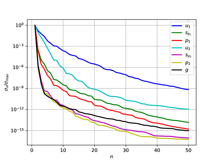
(a) The singular values as a function of the number of POD modes (log scale in $y$–direction)

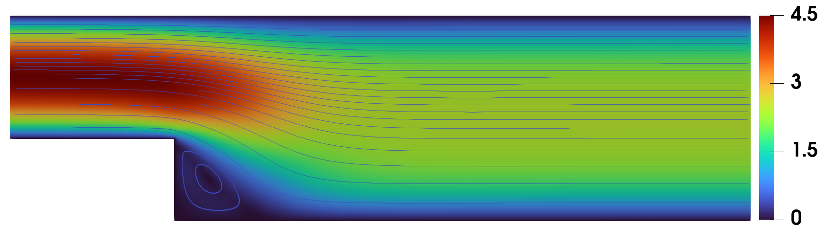
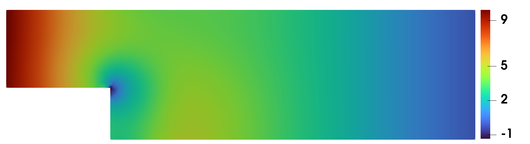
(b) Monolithic model fluid velocity and pressure

Figure 3: Backward–facing step: POD singular eigenvalue decay of the first 50 POD modes (a) and the monolithic solution for a parameter $(\bar{U},\nu)=(4.5,0.4)$ at the final time step (b)

We consider zero initial velocity condition, homogeneous Dirichlet boundary conditions on walls $\Gamma_{wall}$ for the fluid velocity, and homogeneous Neumann conditions on the outlet $\Gamma_{out}$, meaning that we assume free outflow on this portion of the boundary.

We impose a parabolic profile $u_{in}$ on the inlet boundary $\Gamma_{in}$, where $u_{in}(x,y)=\left(w(y),\\ 0\right)^{T}$ with $w(y)=\bar{U}\cdot\frac{4}{9}(y-2)(5-y),\ y\in[2,5]$; the range of $\bar{U}$ is reported in Table 1. Two physical parameters are considered: the viscosity $\nu$ and the maximal magnitude $\bar{U}$ of the inlet velocity profile $u_{in}$. Details of the offline stage and the finite–element discretisation are summarised in Table 1. High–fidelity solutions are obtained by carrying out the minimisation in the space of dimension equal to the number of degrees of freedom at the interface, which is 130 for our test case. The best performance has been achieved by using the limited–memory Broyden–Fletcher–Goldfarb–Shanno (L–BFGS–B) optimisation algorithm [11], where the following stopping criteria were applied: either the maximal number of iteration $\text{it}_{\text{max}}$ is reached or the gradient norm of the target functional is less than the given tolerance $\text{tol}_{\text{opt}}$ or the relative reduction of the functional value is less than the tolerance that is automatically chosen by the scipy library [59].

Snapshots are sampled from a training set of $K$ parameters randomly sampled from the 2–dimensional parameter space for each time–step $t_{i},\,i=1,...,M$, and the first $N_{\text{max}}$ POD modes have been retained for each component. Figure 3(a) shows the POD singular values for all the state and the control variables; we can see an evident exponential decay of the singular values. Figure 3(b) shows an example of a monolithic (whole–domain) solution with which we would conduct a comparison and the numerical analysis of the DD–FOM and the ROM.

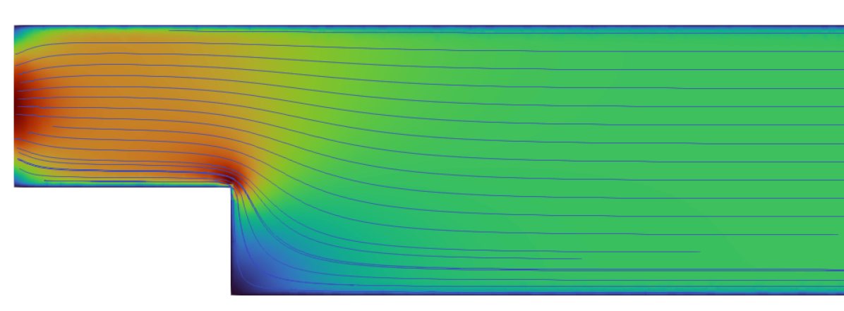
(a) $t=0.01$

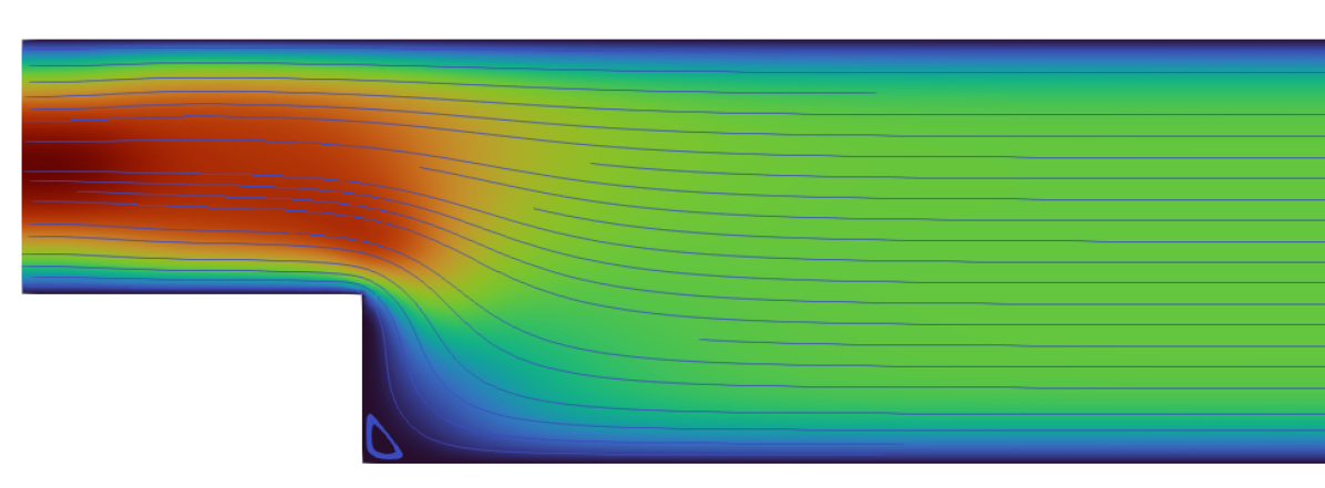
(b) $t=0.25$

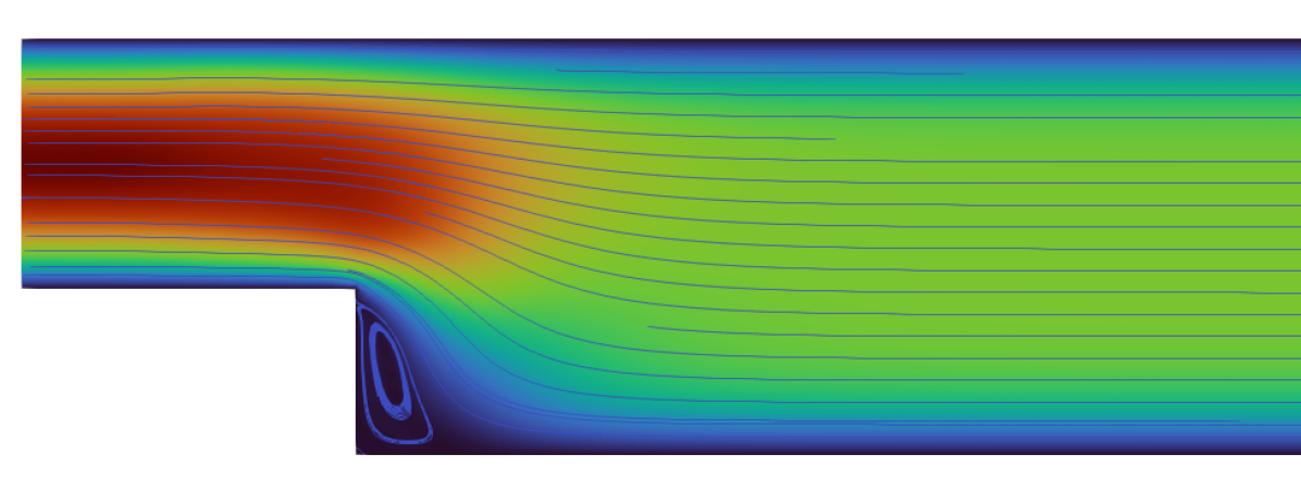
(c) $t=0.5$

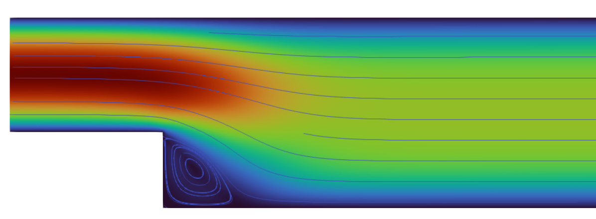
(d) $t=1$

Figure 4: Backward–facing step: high–fidelity solution for the velocities $u_{1}$ and $u_{2}$ at 4 different time instances

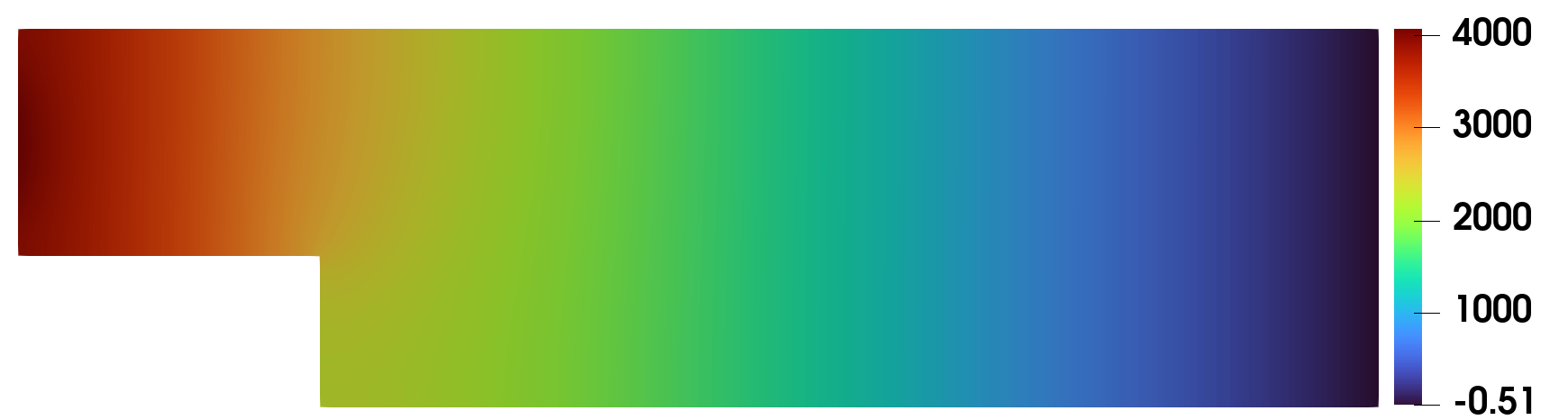
(a) $t=0.01$

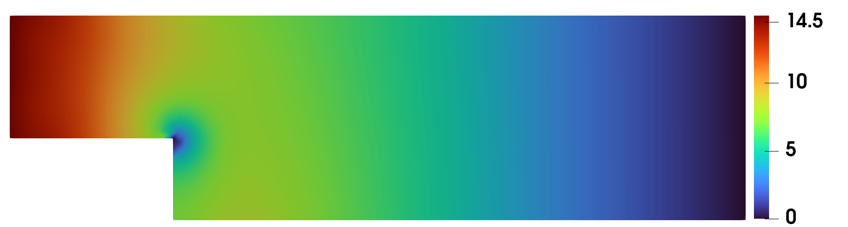
(b) $t=0.25$

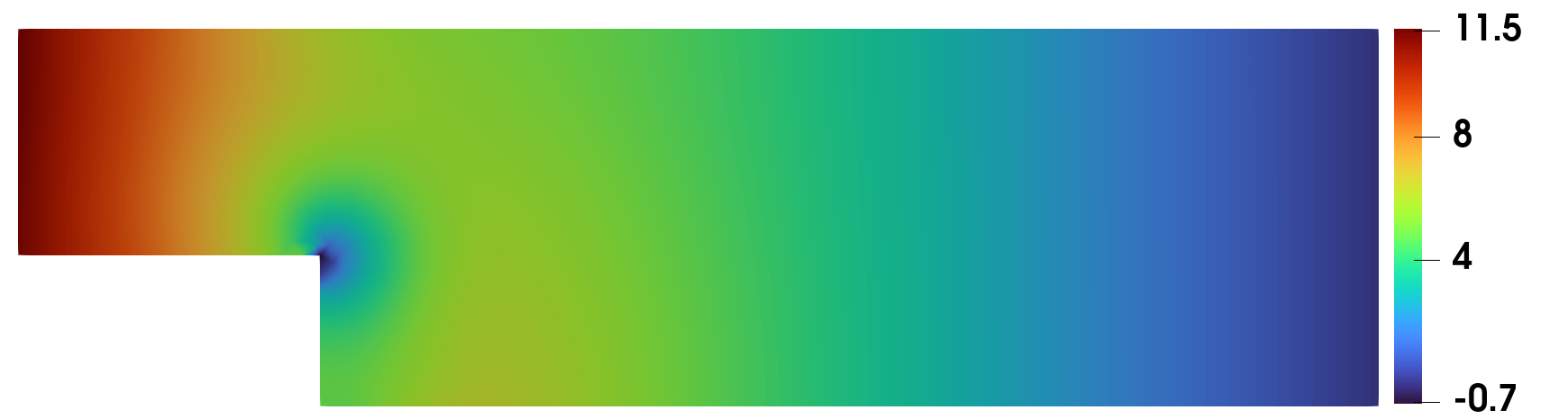
(c) $t=0.5$

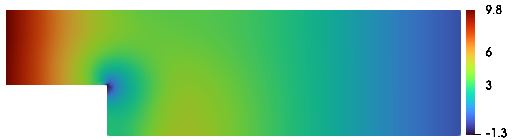
(d) $t=1$

Figure 5: Backward–facing step: high–fidelity solution for the pressures $p_{1}$ and $p_{2}$ at 4 different time instances

Parameter		POD modes
$\nu$	0.4	velocity $u_{1}$	30	pressure $p_{1}$	5	supremiser $s_{1}$	5
$\bar{U}$	4.5	velocity $u_{2}$	12	pressure $p_{2}$	5	supremiser $s_{2}$	5
		control $g$	5

Table 2: Backward–facing step: computational details of the online stage.

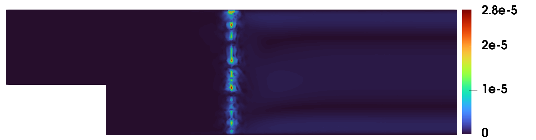
(a) FOM velocity (magnitude)

(b) FOM pressure

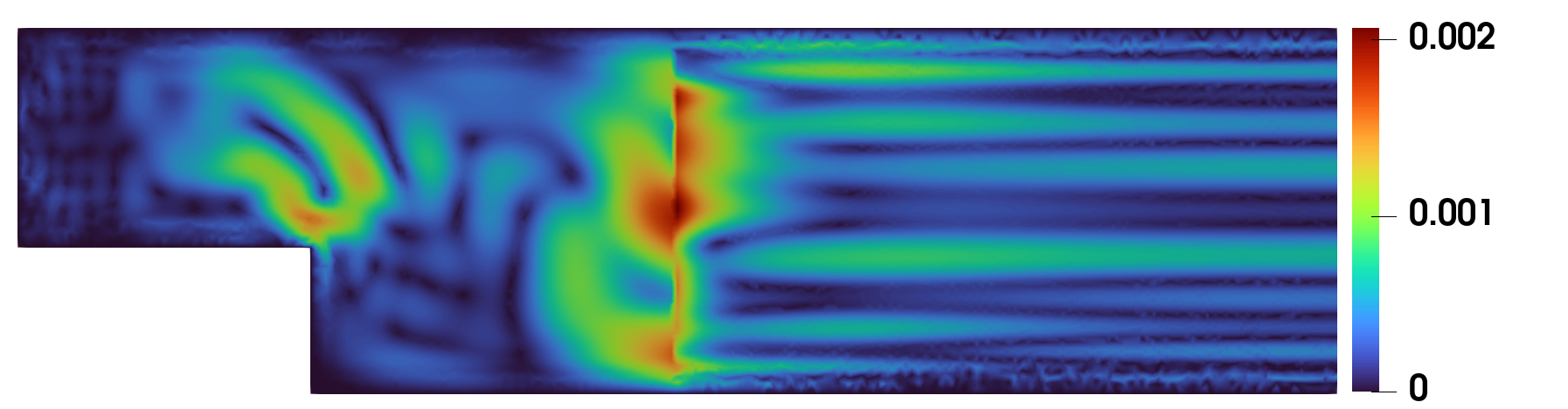
(c) ROM velocity (magnitude)

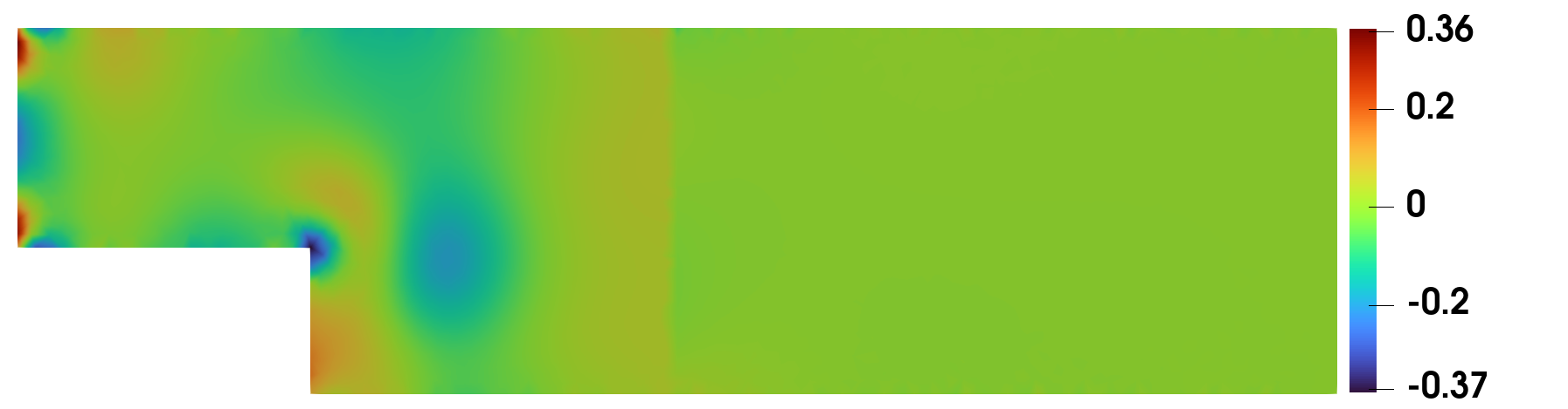
(d) ROM pressure

Figure 6: Backward–facing step: absolute errors of DD–FOM and ROM solutions w.r.t. the monolithic solution at the final time step

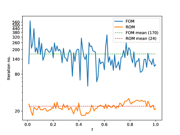
Figure 7: Backward–facing step: number of optimisation iterations of FOM and ROM solvers

(a) Velocity $u_{1}$

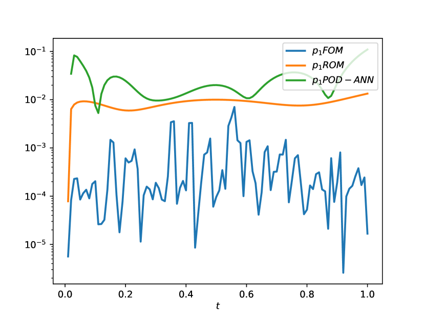
(b) Pressure $p_{1}$

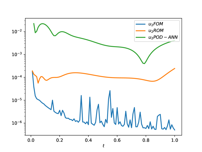
(c) Velocity $u_{2}$

(d) Pressure $p_{2}$

Figure 8: Backward–facing step: relative errors of FOM, ROM and POD–NN solutions w.r.t. the monolithic solution

In Table 2, we list the values of the parameters for which we conduct a numerical test of the ROM and the number of POD modes for each component of the problem. The number of reduced bases is chosen so that the discarded energy for each of the components is less than $10^{-6}$. Reduced–order solutions are obtained by carrying out the minimisation in the space of dimension equal to the number of POD modes for the control $g$, which is 5 for our test case. Clearly, the minimisation in this space of dimension 5 is much simpler than in the FOM one. The optimisation algorithm used in this test case is the same as in the FOM case described above.

Figures 4–5 represent the high–fidelity solutions for a value of the parameters $(\bar{U},\nu)=(4.5,0.4)$ at 4 different time instances. Visually, we can see a great degree of continuity on the interface, which will be highlighted below. Figure 6 shows the spatial distribution of the error with respect to the monolithic solution at the final time step for both the FOM and ROM solutions. As expected, the error of the FOM solution is mostly concentrated at the interface, while ROM contains some extra noise due to the POD reduction.

Figure 7 shows the number of iterations for both FOM and ROM optimisation processes. Each iteration of the optimisation algorithm requires at least one computation of the state and the adjoint solvers. Therefore, we can see that we have managed to obtain a significant reduction in terms of computational efforts: the average number of iterations over all time steps in the case of the FOM solver is 170, while it is 24 in the case of the ROM solver. Additionally, each solver at the reduced level is of much smaller dimension (see Table 2), and with good use of hyper–reduction techniques (see, for instance, [26]), it will allow to obtain very efficient solvers in terms of computational time.

We would like also to provide a comparison of the full–order and the reduced–order models with non–intrusive POD–NN model. Due to the discontinuity with the initial condition, the first time step was excluded from the training set in order to achieve better performance. In practice, this first step can be computed with a Galerkin projection or a FOM step. Figure 8 shows the relative errors with respect to the monolithic solution for the FOM, ROMs and POD–NN model. As we can see, both FOM and ROM give us very good convergence results – the relative error does not exceed 1% in either case. Regarding the POD–NN, in terms of computational time, it is very effective, but the approximation can be very poor, especially in the initial and final time steps. Just to give an idea of the differences in the computational times, one time step of the FOM takes between 30 and 60 minutes, one time step of the ROM (without hyper–reduction) takes around 5 minutes, while a POD–NN prediction needs around $0.003$ seconds. One of the possible scenarios could be a combination of the ROM and the POD–NN model based on the a posteriori error estimates, so that the time steps in which a much more computationally effective ANN model fails to produce a sufficient approximation, the ROM is applied. Similar ideas can be found inter alia in [6]. This will be the subject of future works.

7.2 Lid–driven cavity flow test case

(a) Physical domain

(b) Domain splitting

Figure 9: Lid–driven cavity flow geometry and domain decomposition

In this section, we provide the numerical simulation for the lid–driven cavity flow test case. Figure 9(a) represents the physical domain of interest – the unit square. The split into two domains is performed by dissecting the domain by a median horizontal line as shown in Figure 9(b).

We consider zero initial velocity condition, homogeneous Dirichlet boundary conditions on the boundary $\Gamma_{wall}$ for the fluid velocity and the nonzero horizontal constant velocity on the lid boundary $\Gamma_{lid}$: $u_{lid}=\left(\bar{U},0\right)$; the values of $\bar{U}$ are reported in Table 3.

Physical parameters		FE parameters
Range $\nu$	[1, 1]	Velocity–pressure space in a cell	$\mathbb{P}^{2}\times\mathbb{P}^{1}$
Range $\bar{U}$	[0.5, 5]	Total dofs	58,056
Final time $T$	0.4	Dofs at interface	294
		Time step $\Delta t$	0.01
Optimization		Snapshots training set parameters
Algorithm	L–BFGS–B	Timestep number $M$	40
$\text{it}_{\text{max}}$	300	Parameters training set size $K$	10
$\text{tol}_{\text{opt}}$	$10^{-7}$	Maximum retained modes $N_{\text{max}}$	100

Table 3: Lid–driven cavity flow: computational details of the offline stage.

We consider one physical parameter – the magnitude $\bar{U}$ of the lid velocity profile $u_{in}$. Details of the offline stage and the FE discretisation are summarised in Table 3. High–fidelity solutions are obtained by carrying out the minimisation in the space of dimension equal to the number of degrees of freedom at the interface, which is 294 for our test case.

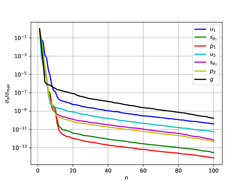
(a) The singular values as a function of the number of POD modes (log scale in $y$–direction)

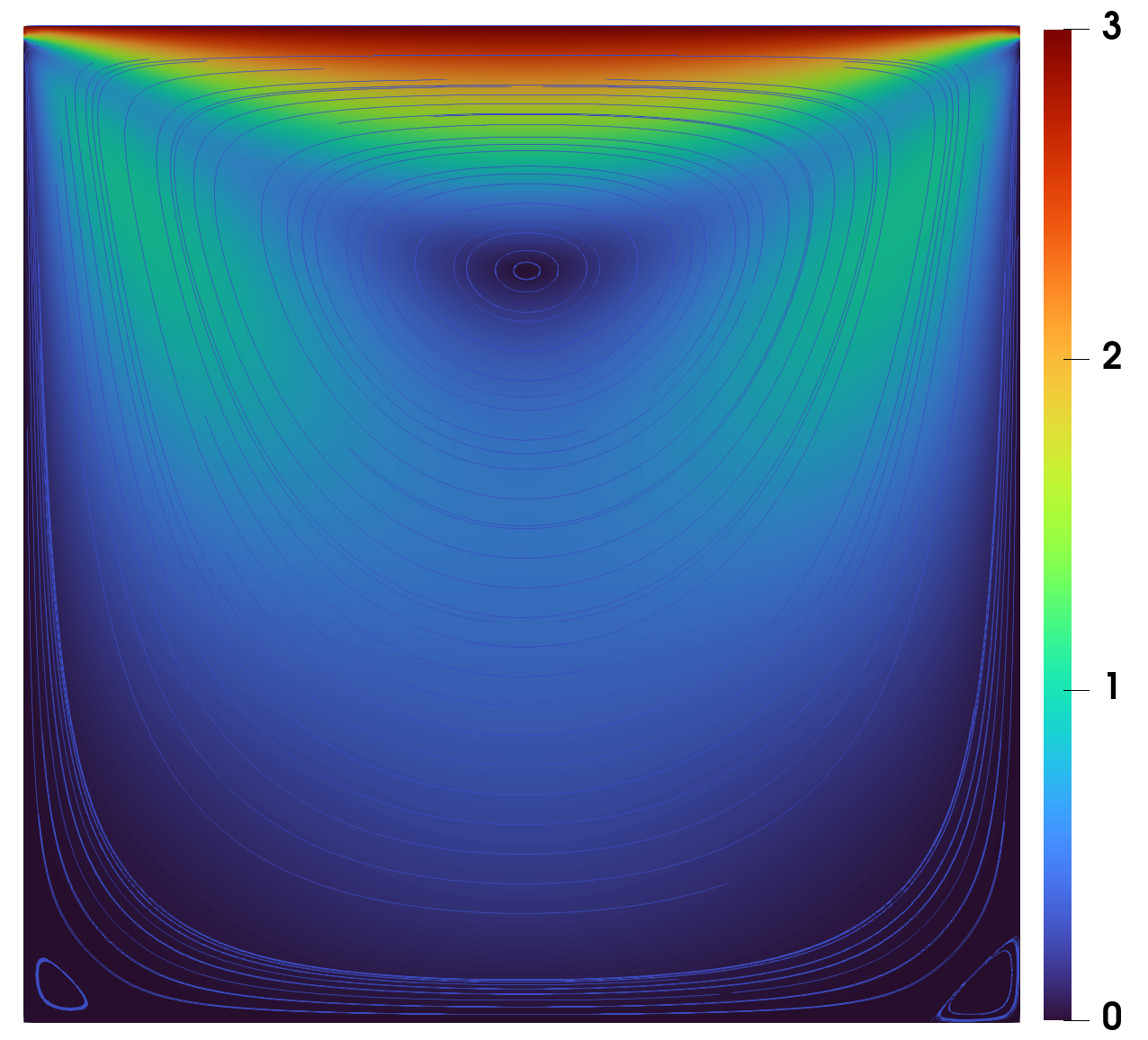
(b) Monolithic model fluid velocity at the final time step

Figure 10: Lid–driven cavity flow: POD singular eigenvalue decay of POD modes (a) and the monolithic solution for a parameter $\bar{U}=3$ at the final time step (b)

(a) $t=0.01$

(b) $t=0.05$

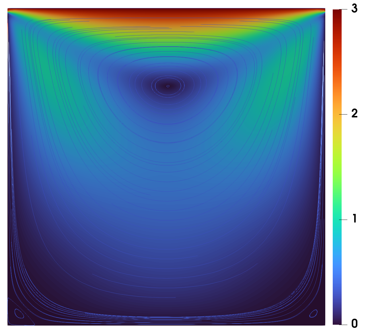
(c) $t=0.4$

Figure 11: Lid–driven cavity flow: FOM velocity solution at 3 different time instances

Snapshots are derived from a training set of $K$ values uniformly sampled from the 1–dimensional parameter space for each time–step $t_{i},\,i=1,...,M$, and the first $N_{max}$ POD modes have been retained for each component. In Figure 10(a), we see that the POD singular values decay even faster than in the previous test for all the state and the control variables. As before, we show in Figure 10(b) the monolithic (whole–domain) solution related to the parameter ($\bar{U}=3$) on which we will test the DD–FOM and the ROM.

Parameter		POD modes
$\nu$	1	velocity $u_{1}$	15	pressure $p_{1}$	10	supremiser $s_{1}$	10
$\bar{U}$	3	velocity $u_{2}$	10	pressure $p_{2}$	10	supremiser $s_{2}$	10
		control $g$	5

Table 4: Lid–driven cavity flow: Computational details of the online stage.

In Table 4 we report the number of POD modes we use to obtain the ROM. The number of reduced bases is chosen so that the discarded energy for each of the components is less than $10^{-6}$. As before, the ROM optimization is the same used in the FOM, but on a smaller space with dimension 5 instead of 294. As an optimisation algorithm in this case we use L–FBGS–B, but in this case, we use a smaller value for $\text{tol}_{\text{opt}}$ of $10^{-6}$.

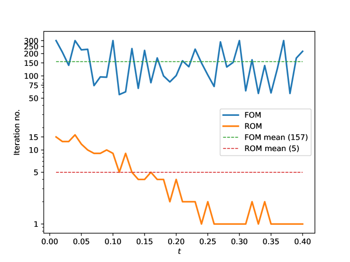
Figure 12: The number of optimisation iterations of FOM and ROM solvers

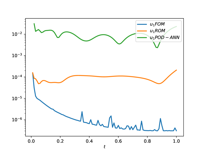
(a) Velocity $u_{1}$

(b) Pressure $p_{1}$

(c) Velocity $u_{2}$

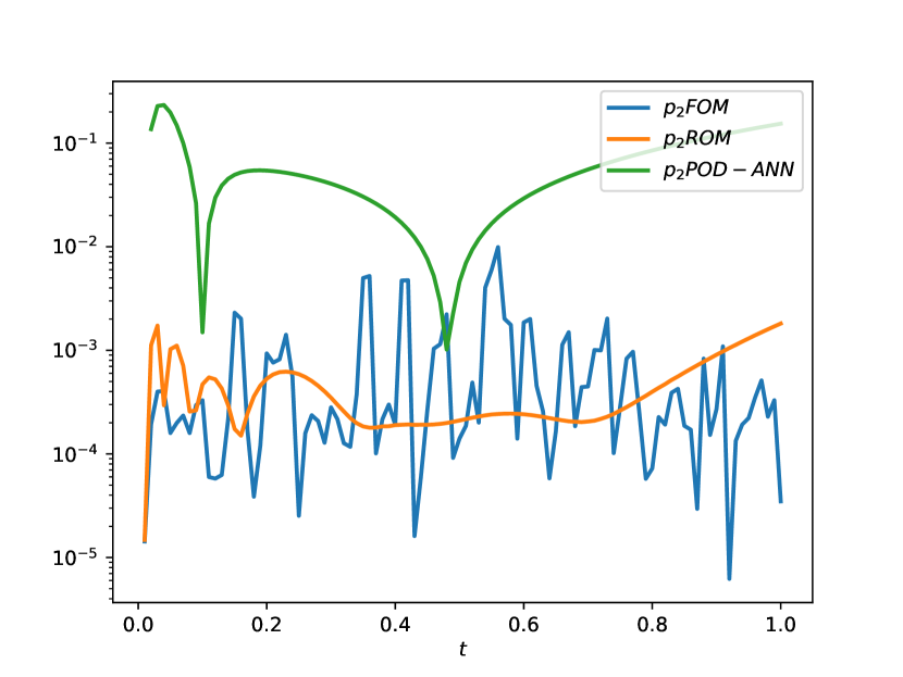
(d) Pressure $p_{2}$

Figure 13: Lid–driven cavity flow: relative errors of FOM, ROM and POD–NN solutions w.r.t. the monolithic solution

Figures 11 represent the DD–FOM solutions for $\bar{U}=3$ at 3 different time instances, where we see a qualitative agreement with the monolithic solution in Figure 10(b).

Again, in Figure 12 we observe that the number of optimization iterations for FOM is between 10 and 100 times larger than the ROM ones. Recalling that each iteration requires at least one computation of the state and the adjoint solvers, we obtain a great computational advantage. For the test with $\bar{U}=3$, the average number of the iteration over all time steps in the case of the FOM solver is 170 while it is 24 in the case of the ROM solver. Additionally, each solver at the reduced level is of a much smaller dimension (see Table 4).

As in the previous test case, we would like to provide a comparison of the full–order and the reduced–order models with non–intrusive POD–NN model. The architecture is still the one reported in Section 6.4 Again, the initial condition leads to a discontinuity in time at the starting timestep, hence, we exclude it from the training set in order to achieve better performance. Figure 13 shows the relative errors with respect to the monolithic solution for the FOM, ROMs and POD–NN model. As we can see, both FOM and ROM give us very good convergence results, i.e., the relative error does not exceed 1% in either case; but, in this case, also POD–NN gives quite good results, indeed, for each variable the relative error does not exceed 3%. Computational times for each method, FOM, ROM and POD–NN, are comparable with those of the backward–facing step flow, that is, one time step of the FOM takes between 15 and 45 minutes, one time step of the ROM (without hyper–reduction) takes on average 5 minutes, while a POD–NN prediction needs around $0.003$ seconds.

8 Conclusions

In this work, we described and conducted the convergence analysis of an optimisation–based domain decomposition algorithm for nonstationary Navier–Stokes equations.

The original problem cast into the optimisation–based domain–decomposition framework leads to the optimal control problem aimed at minimising the coupling error at the interface; the problem, then, has been tackled using an iterative gradient–based optimisation algorithm, which allowed us to obtain a complete separation of the solvers on different subdomains.

At the reduced–order level, we provided two techniques: a POD–Galerkin projection and a data–driven POD–NN, both of them on separate domains. In the Galerkin projection, the optimal–control problem was solved much faster, not only because of the reduced dimensions but also because of the smaller number of iterations. In the POD–NN results are less accurate, but the computational time is way cheaper with respect to the other methods.

As it has been mentioned in the paper, the aforementioned techniques could be promising for various areas of computational physics. First of all, these algorithms can be used when complex time–dependent problems arise and domain decomposition becomes necessary due to the number of degrees of freedom. Moreover, in the context of multi–physics or fluid–structure interaction, the coupling of pre–existing solvers on each subcomponent can be exploited in this framework, with the additional benefit of the reduction for parametric problems, which guarantees high adherence with respect to the full order solutions. Finally, in case the codes are not directly accessible, the presented non–intrusive approach can be used to highly speed up the simulations while still obtaining meaningful results.

References

- [1] FEniCS - the FEniCSx computing platform, https://fenicsproject.org/, 2019.
- [2] RBniCS - reduced order modelling in FEniCS, http://mathlab.sissa.it/rbnics, 2015.
- [3] EZyRB - Easy Reduced Basis method, https://mathlab.sissa.it/ezyrb, 2015.
- [4] S. Ali, F. Ballarin, and G. Rozza. Stabilized reduced basis methods for parametrized steady Stokes and Navier–Stokes equations. Computers & Mathematics with Applications, 80(11):2399–2416, 2020. High-Order Finite Element and Isogeometric Methods 2019.
- [5] M. Astorino, F. Chouly, and M. A. Fernández. Robin Based Semi-Implicit Coupling in Fluid-Structure Interaction: Stability Analysis and Numerics. SIAM Journal on Scientific Computing, 31(6):4041–4065, 2010.
- [6] F. Bai and Y. Wang. A reduced order modeling method based on GNAT-embedded hybrid snapshot simulation. Mathematics and Computers in Simulation, 199:100–132, 2022.
- [7] F. Ballarin, A. Manzoni, A. Quarteroni, and G. Rozza. Supremizer stabilization of POD–Galerkin approximation of parametrized steady incompressible Navier–Stokes equations. International Journal for Numerical Methods in Engineering, 102(5):1136–1161, 2015.
- [8] F. Ballarin and G. Rozza. POD–Galerkin monolithic reduced order models for parametrized fluid-structure interaction problems. International Journal for Numerical Methods in Fluids, 82(12):1010–1034, 2016.
- [9] F. Ballarin, G. Rozza, and Y. Maday. Reduced-order semi-implicit schemes for fluid-structure interaction problems. In Model Reduction of Parametrized Systems, pages 149–167. Springer, 2017.
- [10] C.-H. Bruneau and P. Fabrie. New efficient boundary conditions for incompressible Navier-Stokes equations: a well-posedness result. M2AN - Modélisation mathématique et analyse numérique, 30(7):815–840, 1996.
- [11] R. H. Byrd, P. Lu, J. Nocedal, and C. Zhu. A limited memory algorithm for bound constrained optimization. SIAM Journal on scientific computing, 16(5):1190–1208, 1995.
- [12] G. Carere, M. Strazzullo, F. Ballarin, G. Rozza, and R. Stevenson. A weighted POD-reduction approach for parametrized PDE-constrained Optimal Control Problems with random inputs and applications to environmental sciences. Computers & Mathematics with Applications, 102:261–276, 2021.
- [13] R. Crisovan, D. Torlo, R. Abgrall, and S. Tokareva. Model order reduction for parametrized nonlinear hyperbolic problems as an application to uncertainty quantification. Journal of Computational and Applied Mathematics, 348:466–489, 2019.
- [14] S. Deparis and G. Rozza. Reduced basis method for multi-parameter-dependent steady Navier-Stokes equations: Applications to natural convection in a cavity. Journal of Computational Physics, 228(12):4359–4378, 2009.
- [15] V. Ervin, E. Jenkins, and H. Lee. Approximation of the Stokes–Darcy system by optimization. Journal of Scientific Computing, 59, 06 2014.
- [16] L. Evans. Partial Differential Equations. AMS, 1997.
- [17] A.-L. Gerner and K. Veroy. Certified reduced basis methods for parametrized saddle point problems. SIAM Journal on Scientific Computing, 34(5):A2812–A2836, 2012.
- [18] I. Goodfellow, Y. Bengio, and A. Courville. Deep learning. MIT press, 2016.
- [19] P. Gosselet, V. Chiaruttini, C. Rey, and F. Feyel. A monolithic strategy based on an hybrid domain decomposition method for multiphysic problems. application to poroelasticity. Revue Européenne des Éléments Finis, 13, 04 2012.
- [20] M. Gunzburger and H. K. Lee. A domain decomposition method for optimization problems for partial differential equations. Computers & Mathematics with Applications, 40(2):177–192, 2000.
- [21] M. Gunzburger, J. Peterson, and H. Kwon. An optimization based domain decomposition method for partial differential equations. Computers & Mathematics with Applications, 37(10):77–93, 1999.
- [22] M. D. Gunzburger. Perspectives in Flow Control and Optimization. Society for Industrial and Applied Mathematics, 2002.
- [23] M. D. Gunzburger and H. K. Lee. An optimization-based domain decomposition method for the Navier–Stokes equations. SIAM Journal on Numerical Analysis, 37(5):1455–1480, 2000.
- [24] B. Haasdonk. Reduced Basis Methods for Parametrized PDEs—A Tutorial Introduction for Stationary and Instationary Problems, chapter 2, pages 65–136. Society for Industrial and Applied Mathematics, 2017.
- [25] E. Hairer, S. Nørsett, and G. Wanner. Solving Ordinary Differential Equations I: Nonstiff Problems. Springer-Verlag, Berlin, 1987.
- [26] J. S. Hesthaven, G. Rozza, and B. Stamm. Certified Reduced Basis Methods for Parametrized Partial Differential Equations. Springer Briefs in Mathematics. Springer, Switzerland, 1 edition, 2015.
- [27] J. S. Hesthaven and S. Ubbiali. Non-intrusive reduced order modeling of nonlinear problems using neural networks. Journal of Computational Physics, 363:55–78, 2018.
- [28] M. Hinze, R. Pinnau, M. Ulbrich, and S. Ulbrich. Optimization with PDE Constraints, volume 23 of Mathematical modelling. Springer, 2009.
- [29] T. T. P. Hoang and H. Lee. A global-in-time domain decomposition method for the coupled nonlinear Stokes and Darcy flows. Journal of Scientific Computing, 87, 04 2021.
- [30] D. P. Kingma and J. Ba. Adam: A method for stochastic optimization. arXiv preprint arXiv:1412.6980, 2014.
- [31] P. Kuberry and H. K. Lee. A decoupling algorithm for fluid-structure interaction problems based on optimization. Computer Methods in Applied Mechanics and Engineering, 267:594–605, 2013.
- [32] P. Kuberry and H. K. Lee. Analysis of a fluid-structure interaction problem recast in an optimal control setting. SIAM Journal on Numerical Analysis, 53(3):1464–1487, 2015.
- [33] J. E. Lagnese, G. Leugering, and G. Leugering. Domain in Decomposition Methods in Optimal Control of Partial Differential Equations. Number 148 in International Series of Numerical Mathematics. Springer Science & Business Media, 2004.
- [34] T. Lassila, A. Manzoni, A. Quarteroni, and G. Rozza. Model order reduction in fluid dynamics: challenges and perspectives. In A. Quarteroni and G. Rozza, editors, Reduced Order Methods for Modeling and Computational Reduction, volume 9, pages 235–274. Springer MS&A Series, 2014.
- [35] J. L. Lions and E. Magenes. Non-Homogeneous Boundary Value Problems and Applications. Springer, 1972.
- [36] M. Nonino, F. Ballarin, and G. Rozza. A monolithic and a partitioned reduced basis method for fluid–structure interaction problems. Fluids, 6(6), 2021.
- [37] M. Nonino, F. Ballarin, G. Rozza, and Y. Maday. Projection based semi–implicit partitioned reduced basis method for non parametrized and parametrized Fluid–Structure Interaction problems. Journal of Scientific Computing, 94(4), 2022.
- [38] D. Papapicco, N. Demo, M. Girfoglio, G. Stabile, and G. Rozza. The Neural Network shifted-proper orthogonal decomposition: A machine learning approach for non-linear reduction of hyperbolic equations. Computer Methods in Applied Mechanics and Engineering, 392:114687, 2022.
- [39] F. Pichi, F. Ballarin, G. Rozza, and J. S. Hesthaven. Artificial neural network for bifurcating phenomena modelled by nonlinear parametrized PDEs. PAMM, 20(S1):e202000350, 2021.
- [40] F. Pichi, M. Strazzullo, F. Ballarin, and G. Rozza. Driving bifurcating parametrized nonlinear PDEs by optimal control strategies: application to Navier–Stokes equations with model order reduction. ESAIM: Mathematical Modelling and Numerical Analysis, 56(4):1361–1400, 2022.
- [41] I. Prusak, M. Nonino, D. Torlo, F. Ballarin, and G. Rozza. An optimisation-based domain-decomposition reduced order model for the incompressible Navier-Stokes equations. arXiv preprint arXiv:2211.14528, 2022.
- [42] A. Quarteroni and A. Valli. Numerical Approximation of Partial Differential Equations. Springer Series in Computational Mathematics. 23. Springer Berlin Heidelberg, Heidelberg, DE, 1994. Written for: Numerical analysts, applied mathematicians.
- [43] A. Quarteroni and A. Valli. Domain decomposition Methods for Partial Differential Equations. Oxford University Press, Oxford, UK, 1999.
- [44] T. Richter. Fluid-structure interactions. Lecture Notes in Computational Science and Engineering. Springer International Publishing, Basel, Switzerland, 1 edition, Aug. 2017.
- [45] F. Romor, G. Stabile, and G. Rozza. Non-linear manifold reduced-order models with convolutional autoencoders and reduced over-collocation method. Journal of Scientific Computing, 94(3):74, 2023.
- [46] G. Rozza. Reduced basis methods for stokes equations in domains with non-affine parameter dependence. Computing and Visualization in Science, 12:23–35, 2009.
- [47] G. Rozza, D. Huynh, and A. Patera. Reduced basis approximation and a posteriori error estimation for affinely parametrized elliptic coercive partial differential equations. Archives of Computational Methods in Engineering, 15:1–47, 09 2007.
- [48] P. Siena, M. Girfoglio, and G. Rozza. Fast and accurate numerical simulations for the study of coronary artery bypass grafts by artificial neural networks. In Reduced Order Models for the Biomechanics of Living Organs, pages 167–183. Elsevier, 2023.
- [49] G. Stabile, F. Ballarin, G. Zuccarino, and G. Rozza. A reduced order variational multiscale approach for turbulent flows. Advances in Computational Mathematics, 45(5):2349–2368, 2019.
- [50] G. Stabile and G. Rozza. Finite volume POD-Galerkin stabilised reduced order methods for the parametrised incompressible Navier–Stokes equations. Computers & Fluids, 173:273–284, 2018.
- [51] M. Strazzullo, F. Ballarin, R. Mosetti, and G. Rozza. Model reduction for parametrized optimal control problems in environmental marine sciences and engineering. SIAM Journal on Scientific Computing, 40(4):B1055–B1079, 2018.
- [52] M. Strazzullo, F. Ballarin, and G. Rozza. POD–Galerkin model order reduction for parametrized time dependent linear quadratic optimal control problems in saddle point formulation. Journal of Scientific Computing, 83(3):1–35, 2020.
- [53] M. Strazzullo, F. Ballarin, and G. Rozza. POD-Galerkin model order reduction for parametrized nonlinear time-dependent optimal flow control: an application to shallow water equations. Journal of Numerical Mathematics, 30(1):63–84, 2022.
- [54] M. Strazzullo, M. Girfoglio, F. Ballarin, T. Iliescu, and G. Rozza. Consistency of the full and reduced order models for evolve-filter-relax regularization of convection-dominated, marginally-resolved flows. International Journal for Numerical Methods in Engineering, 123(14):3148–3178, 2022.
- [55] M. Tezzele, N. Demo, G. Stabile, A. Mola, and G. Rozza. Enhancing CFD predictions in shape design problems by model and parameter space reduction. Advanced Modeling and Simulation in Engineering Sciences, 7(1):1–19, 2020.
- [56] D. Torlo, F. Ballarin, and G. Rozza. Stabilized weighted reduced basis methods for parametrized advection dominated problems with random inputs. SIAM/ASA Journal on Uncertainty Quantification, 6(4):1475–1502, 2018.
- [57] D. Torlo and M. Ricchiuto. Model order reduction strategies for weakly dispersive waves. Mathematics and Computers in Simulation, 205:997–1028, 2023.
- [58] L. Venturi, F. Ballarin, and G. Rozza. A weighted POD method for elliptic PDEs with random inputs. Journal of Scientific Computing, 81(1):136–153, 2019.
- [59] P. Virtanen, R. Gommers, T. E. Oliphant, M. Haberland, T. Reddy, D. Cournapeau, E. Burovski, P. Peterson, W. Weckesser, J. Bright, et al. SciPy 1.0: fundamental algorithms for scientific computing in Python. Nature methods, 17(3):261–272, 2020.