Quantification of Predictive Uncertainty via Inference-Time Sampling

Abstract

Predictive variability due to data ambiguities has typically been addressed via construction of dedicated models with built-in probabilistic capabilities that are trained to predict uncertainty estimates as variables of interest. These approaches require distinct architectural components and training mechanisms, may include restrictive assumptions and exhibit overconfidence, i.e., high confidence in imprecise predictions. In this work, we propose a post-hoc sampling strategy for estimating predictive uncertainty accounting for data ambiguity. The method can generate different plausible outputs for a given input and does not assume parametric forms of predictive distributions. It is architecture agnostic and can be applied to any feed-forward deterministic network without changes to the architecture or training procedure. Experiments on regression tasks on imaging and non-imaging input data show the method’s ability to generate diverse and multi-modal predictive distributions, and a desirable correlation of the estimated uncertainty with the prediction error.

1 Introduction

Estimating uncertainty in deep learning (DL) models’ predictions, i.e., predictive uncertainty, is of critical importance in a wide range of applications from diagnosis to treatment planning, e.g., [3]. One generic formulation for predictive uncertainty, i.e., $p(y|x)$, using DL is through the following probabilistic model

$$p(y|x)\triangleq\int_{\mathcal{M}}\int_{\mathcal{D}}\int_{\theta}p(y|x,\theta,\mathcal{D},\mathcal{M})dp(\theta|\mathcal{D},\mathcal{M})dp(\mathcal{D})dp(\mathcal{M}),$$ (1)

where $x,y,\theta,\mathcal{M}$ and $\mathcal{D}$ represent input, output, model parameters, model specification, and training set, respectively. The joint distribution $p(y,\mathcal{D},\mathcal{M},\theta|x)$ is modeled with the factorization $p(y|x,\theta,\mathcal{D},\mathcal{M})p(\theta|\mathcal{D},\mathcal{M})p(\mathcal{D})p(\mathcal{M})$ and $p(y|x)$ is defined through marginalization of $\theta,\mathcal{D}$ and $\mathcal{M}$.

Different components contribute to $p(y|x)$ in the marginalization and represent different sources of uncertainty. Borrowing terminology from [36], $p(y|x,\theta,\mathcal{D},\mathcal{M})$ is often considered as the aleatoric component that models input-output ambiguities, i.e., when the input may not uniquely identify an output [40]. $p(\theta|\mathcal{D},\mathcal{M})$ on the other hand is considered the epistemic component stemming from parameter uncertainty or model bias [8], which can be alleviated by training on more data or using a more appropriate model. Modeling $p(\theta)\triangleq\int_{\mathcal{M}}\int_{\mathcal{D}}p(\theta|\mathcal{M},\mathcal{D})dp(\mathcal{D})dp(\mathcal{M})$ as the epistemic component is also possible, however, this is prohibitively costly in DL models, and therefore mostly not done. Here, we focus on the aleatoric component $p(y|x,\theta,\mathcal{D},\mathcal{M})$ and propose a model agnostic method.

The common approach to model $p(y|x,\theta,\mathcal{D},\mathcal{M})$ in the recent DL literature is to build models that predict probability distributions instead of point-wise predictions. Pioneering this effort, Tanno et al. [35, 36] and Kendall and Gal [20] simultaneously proposed models that output pixel-wise factorized distributions for pixel-wise prediction problems, such as segmentation. Going beyond this simplified factorization, more recent models predict distributions modeling dependencies between multiple outputs, notably for pixel-wise prediction models, such as [23, 2, 39, 38]. These later models are more apt for real world applications as they are capable of producing realistic samples from the modelled $p(y|x,\theta,\mathcal{D},\mathcal{M})$. On the downside, (i) these models require special structures in their architectures, and therefore the principles cannot be easily applied to any top performing architecture without modification, and (ii) they rely on the assumption that input-output ambiguities present in a test sample will be similarly present in the training set, so that models can be trained to predict posterior distributions.

In this work, we propose a novel model for $p(y|x,\theta,\mathcal{D},\mathcal{M})$ and the corresponding Metropolis-Hasting (MH) [16] scheme for sampling of network outputs for a given input, which can be used during inference. We restrict ourselves to problems where a prior model for the outputs, i.e., $p(y)$, can be estimated. While this may seem limiting, on the contrary this restriction is often exploited in medical image analysis to improve model robustness and generalization, e.g., [38, 29, 26, 19]. Inspired by the ideas of network inversion via gradient descent [22] and neural style transfer [12], our main contribution is a new definition of a likelihood function that can be used to evaluate the MH acceptance criterion. The new likelihood function uses input backpropagation and distances in the input space, which (i) makes it architecture agnostic, (ii) does not require access to training or ground truth data, (iii) avoids explicit formulation of analytically described energy functionals, or (iv) implementation of dedicated neural networks (NNs) and training procedures.

We present experiments with two regression problems and compare our method with state-of-the-art methods [11, 39, 30], as well as MC Dropout [11] for completeness, even though it is a method for quantifying epistemic uncertainty. Our experimental evaluation focuses on regression problems, however, the proposed technique can be easily applied to classification problems as well.

2 Related work

Post-hoc uncertainty quantification of trained networks has been previously addressed by Qiu et al. [30]. In their work (RIO), the authors augment a pre-trained deterministic network with a Gaussian process (GP) with a kernel built around the network’s inputs and outputs. The GP can be used for a post-hoc improvement of the network’s outputs and to assess the predictive uncertainty. This model can be applied to any standard NN without modifications. While mathematically elegant and computationally inexpensive, this approach requires access to training data and impose that the posteriors be normally distributed.

One of the dedicated DL models addressing aleatoric uncertainty prediction with an assumption that a prior over outputs $p(y)$ is available is probPCA [39, 38]. Developed for parametric surface reconstruction from images using a principal component analysis (PCA) to define $p(y)$, the method predicts multivariate Gaussian distributions over output mesh vertices, by first predicting posterior distributions over PC representation for a given sample. While the model takes into account covariance structure between vertices, it also requires specific architecture and makes a Gaussian assumption for the posterior.

Sampling techniques built on Monte Carlo integration [15] provide a powerful alternative. Traditional Markov Chain Monte Carlo (MCMC) techniques [27] can construct chains of proposed samples $y^{\prime}$ with strong theoretical guarantees on their convergence to posterior distribution [13]. In MH [16], this is ensured by evaluation of acceptance probabilities. This involves calculation of a prior $p(y^{\prime})$ and a likelihood $L(y^{\prime};x)=p(x|y^{\prime},\theta,\mathcal{D},\mathcal{M})$. At its most explicit form, the evaluation of $L(y^{\prime};x)$ would translate to the generation of plausible inputs for every given $y^{\prime}$ and then calculation of the relative density at the input $x$.

In some applications, the likelihood function can be defined analytically with energy functionals [21, 17, 25]. General DL models, however, do not have convenient closed form formulations that allow analytical likelihood definitions. Defining a tractable likelihood with invertible neural networks [34] or reversible transition kernels [24, 33] is possible, but these approaches require specialized architectures and training procedures. To the best of our knowledge, a solution that can be applied to any pre-trained network has not yet been proposed. Sampling methods without likelihood evaluation, i.e., Approximate Bayesian Computation (ABC) methods [31], can step up to the task, however, they rely on sampling from a likelihood, hence the definition of an appropriate likelihood remains open.

3 Method

We let $f(x|\theta)$ be a deep neural network that is trained on a training set of $(x,y)$ pairs and $\theta$ representing its parameters. The network is trained to predict targets from inputs, i.e., $y\approx f(x|\theta)$. We would like to asses the aleatoric uncertainty $p(y|x,\theta,\mathcal{D},\mathcal{M})$ associated with $f(x|\theta)$. Note that while $f(x|\theta)$ is a deterministic mapping, if there is an input-output ambiguity around an $x$, then a trained model will likely show high sensitivity around that $x$, i.e., predictions will vary greatly with small changes in $x$. We exploit this sensitivity to model $p(y|x,\theta,\mathcal{D},\mathcal{M})$ using $f(x|\theta)$. Such modeling goes beyond a simple sensitivity analysis [32] by allowing drawing realistic samples of $y$ from the modeled distribution.

3.1 Metropolis-Hastings for Target Sampling

Our motivation comes from the well established MH MCMC methods for sampling from a posterior distribution [16]. For a given input $x$ and an initial state $y^{0}$, the MH algorithm generates Markov chains (MC) of states $\{y^{t},t=1,2,\dots,n\}$. At each step $t$ a new proposal is generated $y^{\prime}\sim g(y^{\prime}|y^{t})$ according to a symmetric proposal distribution $g$. The sample is then accepted with the probability

$$A(y^{\prime},y^{t}|x)=\min\bigg{(}1,\underbrace{\frac{g(y^{t}|y^{\prime},x)}{g(y^{\prime}|y^{t},x)}}_{\textrm{transitions}}\underbrace{\frac{p(x|y^{\prime},\theta,\mathcal{D},\mathcal{M})}{p(x|y^{t},\theta,\mathcal{D},\mathcal{M})}}_{\textrm{likelihoods}}\underbrace{\frac{p(y^{\prime})}{p(y^{t})}}_{\textrm{priors}}\bigg{)}$$ (2)

and the next state is set as $y^{t+1}=y^{\prime}$ if the proposal is accepted, and $y^{t+1}=y^{t}$ otherwise. The sufficient condition for asymptotic convergence of the MH MC to the posterior $p(y|x,\theta,\mathcal{D},\mathcal{M})$ is satisfied thanks to the reversibility of transitions $y^{t}\rightarrow y^{t+1}$ [5]. The asymptotic convergence also means that for arbitrary initialization, the initial samples are not guaranteed to come from $p(y|x)$, hence a burn-in period, where initial chain samples are removed, is often implemented [5]. The goal of the acceptance criterion is to reject the unfeasible target proposals $y^{\prime}$ according to prior and likelihood probabilities. The critical part here is that for every target proposal $y^{\prime}$, the prior probability $p(y^{\prime})$ and the likelihood $p(x|y^{\prime})$ needs to be evaluated. While the former is feasible for the problems we focus on, the latter is not trivial to evaluate.

3.2 Likelihood Evaluation

In order to model $p(y|x,\theta,\mathcal{D},\mathcal{M})$, unlike prior work that used a dedicated network architecture, we define a likelihood function $p(x|y,\theta,\mathcal{D},\mathcal{M})$ that can be used with any pre-trained network. Given $f$ and a proposed target $y^{\prime}$, like [7, 6, 10, 28], we define likelihood with an energy function as

$$p(x|y^{\prime},f(\cdot,\theta))\propto\exp(-\beta\,E(x,y^{\prime})),$$ (3)

where $\beta$ is a ”temperature” parameter and $E(x,y^{\prime})$ is evaluated through a process we call gradient descent input backpropagation inspired by neural network inversion approximation in [22] and neural style transfer work [12]. To evaluate $E(x,y^{\prime})$, we generate an input sample $x^{\prime}_{y^{\prime}}$ that is as close as possible to $x$ and lead to the proposed shape $y^{\prime}=f(x^{\prime}_{y^{\prime}}|\theta)$. This action can be formulated as an optimisation problem

$$x^{\prime}_{y^{\prime}}=\mathop{\mathrm{argmin}}\limits_{x^{\prime}}\,\lambda\underbrace{\rho(x^{\prime},x)}_{\textrm{input loss}}+\underbrace{\mu(f(x^{\prime}),y^{\prime})}_{\textrm{target loss}},$$ (4)

where $\rho:\mathcal{X}\times\mathcal{X}\rightarrow\mathbb{R}^{+}$, $\mu:\mathcal{Y}\times\mathcal{Y}\rightarrow\mathbb{R}^{+}$ are distances and $\lambda\in\mathbb{R}$ is a scaling constant ensuring proper optimisation of both loss elements. $\mu$ can be defined as the original distance used for training $f(x|\theta)$. We then define

$$E(x,y^{\prime})\coloneqq\rho(x^{\prime}_{y^{\prime}},x).$$ (5)

We set $\rho(\cdot,x)$ as the squared $L_{2}$ distance in this work, i.e., $\rho(x^{\prime}_{y^{\prime}},x)=\|x^{\prime}_{y^{\prime}}-x\|_{2}^{2}$, but other options are possible, as long as (5) combined with (3) define a proper probability distribution over $x$. Note that the $L_{2}$ distance corresponds to a Gaussian distribution centered around $x^{\prime}_{y^{\prime}}$ as $p(x|y^{\prime},\theta,\mathcal{D},\mathcal{M})$. Even though $p(x|y^{\prime},\theta,\mathcal{D},\mathcal{M})$ is a Gaussian, it is crucial to note that this does not correspond to $p(y|x,\theta,\mathcal{D},\mathcal{M})$ being a Gaussian due to the non-linearity the optimization in Equation 4 introduces. Different $y^{\prime}$’s can lead to very different $x^{\prime}_{y^{\prime}}$, and aggregating the samples through the MH MC process can lead to complex and multi-modal distributions as confirmed by the experiments in Section 4.

Within the MCMC context, the minimisation formulation ensures that we only generate $x^{\prime}_{y^{\prime}}$ close to the test image $x$ that also lead to the proposed $y^{\prime}$ as the prediction. Provided the two terms in (4) are balanced correctly, a low likelihood value assigned to a proposal $y^{\prime}$ indicates $y^{\prime}$ either lies outside the range of $f$ (the trained network is incapable of producing $y^{\prime}$ for any input), or outside of the image (understood as a subset of codomain of $f$) of the inputs similar to $x$ under $f$. On the other hand, a high likelihood value means an $x^{\prime}_{y^{\prime}}$ very close to $x$ can produce $y^{\prime}$ implying the sensitivity of the model around $x$. We can then consider $y^{\prime}$ a sample from $p(y|x,\theta,\mathcal{D},\mathcal{M})$.

The choice of $\beta$ parameter in (3) is important as it affects the acceptance rate in the MH sampling. Correctly setting $\beta$ ensures the acceptance ratio is not dominated by either $p(y)$ or $p(x|y,\theta,\mathcal{D},\mathcal{M})$. The optimisation problem (4) needs to be solved for every MCMC proposal $y^{\prime}$. We will refer to the full proposed MH MCMC sampling scheme as Deep MH.

3.3 Shape Sampling Using Lower Dimensional Representations

As mentioned, we focus on applications where $p(y)$ can be estimated. For low dimensional targets, this can be achieved by parametric or non-parametric models, e.g., KDEs [18]. For high dimensional targets, one can use lower dimensional representations. Here, we illustrate our approach on shape sampling and, as in [39], by using a probabilistic PCA prior for $p(y)$

$$y=US^{\frac{1}{2}}z+\mu+s,$$ (6)

where $U$ is the matrix of principal vectors, $S$ the diagonal principal component matrix and $\mu$ the data mean. All three were precomputed using surfaces in the training set of $f$. PCA coefficients $z$ and global shift $s$ then modulate and localise the shape in space, respectively. The posterior $p(y|x,\theta,\mathcal{D},\mathcal{M})$ is then approximated by deploying the MH sampling process to estimate the joint posterior of the parameterisation $p(z,s|x,\theta,\mathcal{D},\mathcal{M})$. Proposal shapes $y^{\prime}$ are constructed at every step of the MCMC from proposals $z^{\prime}$ and $s^{\prime}$ for the purposes of likelihood computation as defined by (3) and (5). PCA coefficients and shifts are assumed to be independently distributed. We set $p(z)=\mathcal{N}(z;0,I)$ as in [4] and $p(s)=\mathcal{U}([0,D]^{2})$ for an input image $x\in\mathbb{R}^{D\times D}$. In practice, we restrict the prior on shift to a smaller area within the image to prevent the accepted shapes from crossing the image boundaries. Assuming both proposals are symmetrical Gaussian, the MH acceptance criterion (2) then becomes $A((z^{\prime},s^{\prime}),(z^{t},s^{t})|x)=\min\left(1,{\frac{p(x|z^{\prime},s^{\prime},f(\cdot;\theta))}{p(x|z^{t},s^{t},f(\cdot;\theta))}}\frac{p(z^{\prime})}{p(z^{t})}\frac{p(s^{\prime})}{p(s^{t})}\right)$.

4 Results

The method was compared against three uncertainty quantification baselines: (1) Post-hoc uncertainty estimation method RIO [30], using the code provided by the authors; and Dedicated probabilistic forward systems: (2) probPCA [38] and (3) MC Dropout [11]. We compare with MC dropout to provide a complete picture even though it is quantifying epistemic uncertainty.

We evaluate the uncertainty estimates on two regression problems on imaging and non-imaging data. The first is left ventricle myocardium surface delineation in cardiac MR images from the UK BioBank data set [1] where network $f:\mathbb{R}^{D}\times\mathbb{R}^{D}\rightarrow\mathbb{R}^{50\times 2}$ predicts coordinates of 50 vertices on the surface in small field of view (SFOV) and large FOV (LFOV) images for $D=60,200$, respectively. The data sets are imbalanced when it comes to location and orientation of the images with propensity towards the myocardium being in the central area of the image (90% of the examples). We tested the method on a 10-layer CNN trained to predict a lower dimensional PCA representation from images, as described in Sec. 3.3 and proposed in [26], which is a deterministic version of probPCA. The CNN predicts 20 PCA components which are then transformed into a surface with 50 vertices. The second is a 1D problem of computed tomography (CT) slice localisation within the body given the input features describing the tissue content via histograms in polar space [14, 9] and $f:\mathbb{R}^{384}\rightarrow[0,100]$. We use the same data set and training setup as in the original RIO paper [30] and tested the method on a fully connected network with 2 hidden layers.

The same base architectures were used across baselines, with method pertinent modifications where needed, following closely the original articles [39, 11]. No data augmentation was used for forward training. Hyperparameter search for Deep MH was done on the validation set by hand tuning or grid search to get a good balance between the proper optimisation of (4), good convergence times and optimal acceptance rates (average of $\sim 20\%$ for high and $\sim 40\%$ for the one-dimensional tasks). This led to $\beta$ = 10000 (SFOV), 30000 (LFOV), 60000 (CT) and Gaussian proposal distributions: $z^{\prime}\sim\mathcal{N}(z^{t},\sigma_{z}^{2}I)$ and $s^{\prime}\sim\mathcal{N}(s^{t},\sigma_{s}^{2}I)$, with ($\sigma_{z}$, $\sigma_{s}$) = (0.1, 2) in SFOV, and (0.2, 8) in LFOV; in CT $y^{\prime}\sim\mathcal{N}(y^{t},I)$. Choice of priors for the delineation task followed Sec. 3.3. In CT, we used an uniformative prior $\mathcal{U}([0,100])$ to reflect that the testing slice can lie anywhere in the body. Parameters of the input backpropagation were set to $\lambda=1$ and $\sigma_{n}=0.1$. We employed independent chain parallelization to speed up sampling and reduce auto-correlation within the sample sets. Chains were initialised randomly and run for a fixed number of steps with initial burn in period removed based on convergence of trace plots of the sampled target variables. The final posteriors were then approximated by aggregation of the samples across the chains. For comparisons, we quantify uncertainty in the system via dispersion of $p(y|x,\theta,\mathcal{D},\mathcal{M})$: standard deviation $\sigma_{y|x}$ in 1D problems; trace of the covariance matrix $\Sigma_{y|x}$ in multi-dimensional tasks (sample covariance matrix for Deep MH and MC Dropout, and predictive covariance for probPCA).

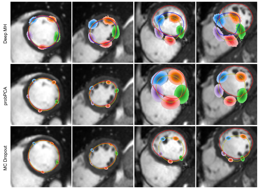
Figure 1: Comparison of estimated $p(y|x,\theta,\mathcal{D},\mathcal{M})$ for selected test subjects: GT shape (red), forward prediction $f(x_{i}|\theta)$ (blue), sample / predicted mean (yellow). Kernel density estimates were used for visualization. Only 5 vertices were visualised for clarity. Test subjects are ordered column-wise according to growing fixed network prediction error ($\textrm{RMSE}(f(x),y_{\textrm{GT}})=0.48;2.72;5.25;6.31$; test set average $\textrm{RMSE}=1.46$). Outlier test subjects (column 3-4) are associated with higher uncertainty and lower accuracy for all methods.

Predictive Posteriors: Fig. 1 shows qualitative comparison of target distributions produced by Deep MH, MC Dropout and probPCA in the SFOV surface reconstruction task. We include two images representative of the majority of the data set (well centered) and two from the 10% outlier group (images with large translation and/or reflection compared to rest of the data set). The posteriors obtained by Deep MH exhibited greater variability, including multimodality, than the baseline methods even for the test images with lower forward prediction RMSE. In contrast, probPCA produced unimodal Gaussians, expectedly. MC Dropout, at $p=0.5$, produced tight distributions around the sample mean.

Deep MH posteriors also showed a larger dispersion of vertex locations along the surface as can be seen in the first two columns. This uncertainty reflects the ambiguity in the target generation process. Boundaries seen in the images can identify the placement of a vertex in the orthogonal direction to the boundary, but placement along the boundary is much less obvious and variable. Deep MH posteriors captured this ambiguity well while others were not able to do so. Irrespective of the method, the high probability regions of the predicted $p(y|x,\theta,\mathcal{D},\mathcal{M})$ might not cover the GT shapes when the prediction fails, as can be seen in the last two columns of Fig. 1.

Correlation with accuracy: We investigated the relationship between accuracy of a network and the predictive uncertainty. A good uncertainty estimation model should yield a non-decreasing relationship between uncertainty and prediction accuracy, and not show overconfidence, i.e., assign high confidence to imprecise predictions.

	Spearman [r;p]	Pearson [r;p]	Spearman [r;p]	Pearson [r;p]
Method	Shape delineation SFOV: full		Shape delineation SFOV: homogeneous
Deep MH	$0.30$; $3\times 10^{-3}$	$0.62$; $1\times 10^{-11}$	$0.26$; $2\times 10^{-2}$	$0.38$;$3\times 10^{-4}$
probPCA	$0.35$; $5\times 10^{-4}$	$0.57$; $8\times 10^{-10}$	$0.19$; $8\times 10^{2}$	$0.40$; $9\times 10^{-5}$
MC Dropout	$0.34$; $5\times 10^{-4}$	$0.61$; $3\times 10^{-11}$	$0.21$; $5\times 10^{2}$	$0.29$; $7\times 10^{-3}$
Method	Shape delineation LFOV: full		Shape delineation LFOV: homogeneous
Deep MH	$0.33$; $3\times 10^{-3}$	$0.38$; $7\times 10^{-4}$	$0.20$; $9\times 10^{-2}$	$0.26$; $3\times 10^{-2}$
probPCA	$0.17$; $1\times 10^{-2}$	$0.33$; $3\times 10^{-3}$	$0.04$; $7\times 10^{-1}$	$0.03$; $8\times 10^{-1}$
MC Dropout	$0.52$; $9\times 10^{-7}$	$0.55$; $2\times 10^{-7}$	$0.42$; $2\times 10^{-4}$	$0.42$; $2\times 10^{-4}$
Method	CT slice localisation
Deep MH	$0.55$; $1\times 10^{-7}$	$0.64$; $2\times 10^{-9}$
RIO	$0.07$; $6\times 10^{-1}$	$0.13$; $3\times 10^{-1}$
MC Dropout	$0.53$; $2\times 10^{-6}$	$0.51$; $7\times 10^{-6}$

Table 1: Correlation between uncertainty and accuracy (RMSE).

Tab. 1 presents the correlation coefficients between quantified uncertainties and the accuracy (RMSE) of either the forward prediction of the pre-trained network in the case of Deep MH, or predictive mean for the baselines. We include results for the shape delineation task analysed in two settings: on the full imbalanced test sets, and on the homogeneous subsets of the test sets with two outliers, detected manually, removed. Deep MH yielded higher Spearman and Pearson’s correlation for most cases than probPCA and RIO. Correlation of epistemic uncertainty, as quantified by MC Dropout, with prediction error was higher in some cases than that of aleatoric uncertainty quantified by Deep MH.

Further analysis together with additional in-depth tests can be found in [37].

5 Conclusion

In this work we proposed a novel method—Deep MH—for uncertainty estimation of trained deterministic networks using MH MCMC sampling. The method is architecture agnostic and does not require training of any dedicated NNs or access to training or GT data. Experiments on regression tasks showed the better quality of the Deep MH uncertainty estimates not only in comparison to a post-hoc baseline [30], but dedicated probabilistic forward models as well  [39, 38].

The main limitation of Deep MH is its computational complexity. Some of it stems from its sampling nature. The rest is due to the proposed evaluation of the likelihood. A possible alternative to the proposed likelihood computation via optimisation is the simulation of an inversion process via a generative adversarial network (GAN), which would, however, involve a design of an additional dedicated network. Deep MH can be applied to problems where it is possible to define or estimate a prior distribution $p(y)$. While the deployment to problems with higher dimensional targets is an open research question, it is straightforward for problems with low effective dimensions. These are commonly found across the spectrum of the deep learning applications.

5.0.1 Acknowledgements

This research has been conducted using the UK Biobank Resource under Application Number 17806.

References

- [1] Uk biobank homepage. https://www.ukbiobank.ac.uk/about-biobank-uk, 24 May 2021
- [2] Baumgartner, C.F., Tezcan, K.C., Chaitanya, K., Hötker, A.M., Muehlematter, U.J., Schawkat, K., Becker, A.S., Donati, O., Konukoglu, E.: Phiseg: Capturing uncertainty in medical image segmentation. In: Shen, D., Liu, T., Peters, T.M., Staib, L.H., Essert, C., Zhou, S., Yap, P.T., Khan, A. (eds.) Medical Image Computing and Computer Assisted Intervention – MICCAI 2019. pp. 119–127. Springer International Publishing, Cham (2019)
- [3] Begoli, E., Bhattacharya, T., Kusnezov, D.: The need for uncertainty quantification in machine-assisted medical decision making. Nature Machine Intelligence 1(1), 20–23 (Jan 2019). https://doi.org/10.1038/s42256-018-0004-1, https://doi.org/10.1038/s42256-018-0004-1
- [4] Bishop, C.M.: Pattern Recognition and Machine Learning (Information Science and Statistics). Springer-Verlag, Berlin, Heidelberg (2006)
- [5] Brooks, S., Gelman, A., Jones, G., Meng, X.L.: Handbook of Markov Chain Monte Carlo. CRC press (2011)
- [6] Chang, J., Fisher, J.W.I.: Efficient mcmc sampling with implicit shape representations. In: CVPR. pp. 2081–2088. IEEE Computer Society (2011), http://dblp.uni-trier.de/db/conf/cvpr/cvpr2011.html$#$ChangF11
- [7] Chen, S., Radke, R.J.: Markov chain monte carlo shape sampling using level sets. In: 2009 IEEE 12th International Conference on Computer Vision Workshops, ICCV Workshops. pp. 296–303 (2009). https://doi.org/10.1109/ICCVW.2009.5457687
- [8] Draper, D.: Assessment and propagation of model uncertainty. Journal of the Royal Statistical Society. Series B (Methodological) 57(1), 45–97 (1995), http://www.jstor.org/stable/2346087
- [9] Dua, D., Graff, C.: UCI machine learning repository (2017), http://archive.ics.uci.edu/ml
- [10] Erdil, E., Yildirim, S., Çetin, M., Tasdizen, T.: Mcmc shape sampling for image segmentation with nonparametric shape priors. In: 2016 IEEE Conference on Computer Vision and Pattern Recognition (CVPR). pp. 411–419 (2016). https://doi.org/10.1109/CVPR.2016.51
- [11] Gal, Y., Ghahramani, Z.: Dropout as a bayesian approximation: Representing model uncertainty in deep learning. In: Balcan, M.F., Weinberger, K.Q. (eds.) Proceedings of The 33rd International Conference on Machine Learning. Proceedings of Machine Learning Research, vol. 48, pp. 1050–1059. PMLR, New York, New York, USA (20–22 Jun 2016), http://proceedings.mlr.press/v48/gal16.html
- [12] Gatys, L.A., Ecker, A.S., Bethge, M.: Image style transfer using convolutional neural networks. In: Proceedings of the IEEE Conference on Computer Vision and Pattern Recognition (CVPR) (June 2016)
- [13] Gelman, A., Carlin, J.B., Stern, H.S., Rubin, D.B.: Bayesian Data Analysis. Chapman and Hall/CRC, 2nd ed. edn. (2004)
- [14] Graf, F., Kriegel, H., Schubert, M., Pölsterl, S., Cavallaro, A.: 2d image registration in CT images using radial image descriptors. In: Fichtinger, G., Martel, A.L., Peters, T.M. (eds.) Medical Image Computing and Computer-Assisted Intervention - MICCAI 2011 - 14th International Conference, Toronto, Canada, September 18-22, 2011, Proceedings, Part II. Lecture Notes in Computer Science, vol. 6892, pp. 607–614. Springer (2011). https://doi.org/10.1007/978-3-642-23629-7_74, https://doi.org/10.1007/978-3-642-23629-7_74
- [15] Hammersley, J.M., Handscomb, D.C.: Monte Carlo methods / [by] J.M. Hammersley and D.C. Handscomb. Methuen London (1964)
- [16] Hastings, W.K.: Monte carlo sampling methods using markov chains and their applications. Biometrika 57(1), 97–109 (1970), http://www.jstor.org/stable/2334940
- [17] Houhou, N., Thiran, J.P., Bresson, X.: Fast texture segmentation model based on the shape operator and active contour. In: 2008 IEEE Conference on Computer Vision and Pattern Recognition. pp. 1–8 (2008). https://doi.org/10.1109/CVPR.2008.4587449
- [18] Izenman, A.J.: Modern multivariate statistical techniques. Regression, classification and manifold learning 10, 978–0 (2008)
- [19] Karani, N., Erdil, E., Chaitanya, K., Konukoglu, E.: Test-time adaptable neural networks for robust medical image segmentation. Medical Image Analysis 68, 101907 (2021). https://doi.org/https://doi.org/10.1016/j.media.2020.101907, https://www.sciencedirect.com/science/article/pii/S1361841520302711
- [20] Kendall, A., Gal, Y.: What uncertainties do we need in bayesian deep learning for computer vision? In: Guyon, I., von Luxburg, U., et al. (eds.) Advances in Neural Information Processing Systems 30: Annual Conference on Neural Information Processing Systems 2017, 4-9 December 2017, Long Beach, CA, USA. pp. 5574–5584 (2017)
- [21] Kim, J., Fisher, J.W., III, Yezzi, A., Çetin, M., Willsky, A.S.: A nonparametric statistical method for image segmentation using information theory and curve evolution. IEEE TRANSACTIONS ON IMAGE PROCESSING 14(10), 1486–1502 (2005)
- [22] Kindermann, J., Linden, A.: Inversion of neural networks by gradient descent. Parallel Computing 14(3), 277–286 (1990). https://doi.org/https://doi.org/10.1016/0167-8191(90)90081-J, https://www.sciencedirect.com/science/article/pii/016781919090081J
- [23] Kohl, S., Romera-Paredes, B., Meyer, C., De Fauw, J., Ledsam, J.R., Maier-Hein, K., Eslami, S.M.A., Jimenez Rezende, D., Ronneberger, O.: A probabilistic u-net for segmentation of ambiguous images. In: Bengio, S., Wallach, H., Larochelle, H., Grauman, K., Cesa-Bianchi, N., Garnett, R. (eds.) Advances in Neural Information Processing Systems. vol. 31. Curran Associates, Inc. (2018), https://proceedings.neurips.cc/paper/2018/file/473447ac58e1cd7e96172575f48dca3b-Paper.pdf
- [24] Levy, D., Sohl-dickstein, J., Hoffman, M.: Generalizing hamiltonian monte carlo with neural networks (2018), https://openreview.net/pdf?id=B1n8LexRZ, iCLR 2018
- [25] Michailovich, O., Rathi, Y., Tannenbaum, A.: Image segmentation using active contours driven by the bhattacharyya gradient flow. IEEE Transactions on Image Processing 16(11), 2787–2801 (2007). https://doi.org/10.1109/TIP.2007.908073
- [26] Milletari, F., Rothberg, A., Jia, J., Sofka, M.: Integrating statistical prior knowledge into convolutional neural networks. In: Descoteaux, M., Maier-Hein, L., et al. (eds.) Medical Image Computing and Computer Assisted Intervention - MICCAI 2017 - 20th International Conference, Quebec City, QC, Canada, September 11-13, 2017, Proceedings, Part I. Lecture Notes in Computer Science, vol. 10433, pp. 161–168. Springer (2017)
- [27] Neal, R.M.: Probabilistic inference using Markov chain Monte Carlo methods. Tech. Rep. CRG-TR-93-1, Dept. of Computer Science, University of Toronto (1993)
- [28] Neal, R.M.: Bayesian learning for neural networks, vol. 118. Springer Science & Business Media (2012)
- [29] Oktay, O., Ferrante, E., Kamnitsas, K., Heinrich, M., Bai, W., Caballero, J., Cook, S.A., de Marvao, A., Dawes, T., O‘Regan, D.P., Kainz, B., Glocker, B., Rueckert, D.: Anatomically constrained neural networks (acnns): Application to cardiac image enhancement and segmentation. IEEE Transactions on Medical Imaging 37(2), 384–395 (2018). https://doi.org/10.1109/TMI.2017.2743464
- [30] Qiu, X., Meyerson, E., Miikkulainen, R.: Quantifying point-prediction uncertainty in neural networks via residual estimation with an I/O kernel. In: 8th International Conference on Learning Representations, ICLR 2020, Addis Ababa, Ethiopia, April 26-30, 2020. OpenReview.net (2020), https://openreview.net/forum?id=rkxNh1Stvr
- [31] Rubin, D.B.: Bayesianly Justifiable and Relevant Frequency Calculations for the Applied Statistician. The Annals of Statistics 12(4), 1151 – 1172 (1984). https://doi.org/10.1214/aos/1176346785, https://doi.org/10.1214/aos/1176346785
- [32] Saltelli, A., Tarantola, S., Campolongo, F., Ratto, M., et al.: Sensitivity analysis in practice: a guide to assessing scientific models. Chichester, England (2004)
- [33] Song, J., Zhao, S., Ermon, S.: A-nice-mc: Adversarial training for mcmc. In: Guyon, I., Luxburg, U.V., Bengio, S., Wallach, H., Fergus, R., Vishwanathan, S., Garnett, R. (eds.) Advances in Neural Information Processing Systems. vol. 30. Curran Associates, Inc. (2017), https://proceedings.neurips.cc/paper/2017/file/2417dc8af8570f274e6775d4d60496da-Paper.pdf
- [34] Song, Y., Meng, C., Ermon, S.: Mintnet: Building invertible neural networks with masked convolutions. In: Wallach, H., Larochelle, H., Beygelzimer, A., d'Alché-Buc, F., Fox, E., Garnett, R. (eds.) Advances in Neural Information Processing Systems. vol. 32. Curran Associates, Inc. (2019), https://proceedings.neurips.cc/paper/2019/file/70a32110fff0f26d301e58ebbca9cb9f-Paper.pdf
- [35] Tanno, R., Worrall, D.E., Ghosh, A., Kaden, E., Sotiropoulos, S.N., Criminisi, A., Alexander, D.C.: Bayesian image quality transfer with cnns: Exploring uncertainty in dmri super-resolution. In: Descoteaux, M., Maier-Hein, L., Franz, A., Jannin, P., Collins, D.L., Duchesne, S. (eds.) Medical Image Computing and Computer Assisted Intervention-MICCAI 2017. pp. 611–619. Springer International Publishing, Cham (2017)
- [36] Tanno, R., Worrall, D.E., Kaden, E., Ghosh, A., Grussu, F., Bizzi, A., Sotiropoulos, S.N., Criminisi, A., Alexander, D.C.: Uncertainty modelling in deep learning for safer neuroimage enhancement: Demonstration in diffusion mri. NeuroImage 225, 117366 (2021). https://doi.org/https://doi.org/10.1016/j.neuroimage.2020.117366, https://www.sciencedirect.com/science/article/pii/S1053811920308521
- [37] Tóthová, K.: On Predicting with Aleatoric Uncertainty in Deep Learning. Ph.D. thesis, ETH Zurich (2022). https://doi.org/doi = https://doi.org/10.1016/j.media.2020.101907
- [38] Tóthová, K., Parisot, S., Lee, M., Puyol-Antón, E., King, A., Pollefeys, M., Konukoglu, E.: Probabilistic 3d surface reconstruction from sparse mri information. In: Martel, A.L., Abolmaesumi, P., Stoyanov, D., Mateus, D., Zuluaga, M.A., Zhou, S.K., Racoceanu, D., Joskowicz, L. (eds.) Medical Image Computing and Computer Assisted Intervention – MICCAI 2020. pp. 813–823. Springer International Publishing, Cham (2020)
- [39] Tóthová, K., Parisot, S., Lee, M.C.H., Puyol-Antón, E., Koch, L.M., King, A.P., Konukoglu, E., Pollefeys, M.: Uncertainty quantification in cnn-based surface prediction using shape priors. In: Reuter, M., Wachinger, C., Lombaert, H., Paniagua, B., Lüthi, M., Egger, B. (eds.) Shape in Medical Imaging. pp. 300–310. Springer International Publishing, Cham (2018)
- [40] Wang, H., Levi, D.M., Klein, S.A.: Intrinsic uncertainty and integration efficiency in bisection acuity. Vision Research 36(5), 717–739 (1996). https://doi.org/https://doi.org/10.1016/0042-6989(95)00143-3, https://www.sciencedirect.com/science/article/pii/0042698995001433