Measurement-Induced Criticality is Tomographically Optimal
Ahmed A. Akhtar
Department of Physics, University of California San Diego, La Jolla, CA 92093, USA
Hong-Ye Hu
Department of Physics, Harvard University, 17 Oxford Street, Cambridge, MA 02138, USA
Harvard Quantum Initiative, Harvard University, 17 Oxford Street, Cambridge, MA 02138, USA
Yi-Zhuang You
Department of Physics, University of California San Diego, La Jolla, CA 92093, USA
Abstract
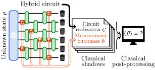
We develop a classical shadow tomography protocol utilizing the randomized measurement scheme based on hybrid quantum circuits, which consist of layers of two-qubit random unitary gates mixed with single-qubit random projective measurements. Unlike conventional protocols that perform all measurements by the end of unitary evolutions, our protocol allows measurements to occur at any spacetime position throughout the quantum evolution. We provide a universal classical post-processing strategy to approximately reconstruct the original quantum state from intermittent measurement outcomes given the corresponding random circuit realizations over repeated experiments. We investigated the sample complexity for estimating different observables at different measurement rates of the hybrid quantum circuits. Our result shows that the sample complexity has an optimal scaling at the critical measurement rate when the hybrid circuit undergoes the measurement-induced transition.
pacs:
Valid PACS appear here
Classical shadow tomography Huang et al. (2020); Ohliger et al. (2013); Guta et al. (2020) offers an efficient randomized measurement scheme for extracting physically relevant information from a quantum state. Much research Huang et al. (2021); Hadfield et al. (2022); Elben et al. (2020); Enshan Koh and Grewal (2022); Hu and You (2022); Hu et al. (2023); Levy et al. (2021); Bu et al. (2022); Hu et al. (2022); Seif et al. (2022); Hao Low (2022); Akhtar et al. (2023); Bertoni et al. (2022); Arienzo et al. (2022); Ippoliti et al. (2023) primarily concentrates on the randomized measurement protocol that entails random unitary evolution, followed by the final stage of local measurements on all qubits. This process is akin to halting the universe’s time evolution to measure every qubit. A more realistic measurement scheme involves conducting local measurements intermittently while the entire quantum system continues to evolve, which more closely imitates how we observe the quantum universe surrounding us. This situation can be represented by hybrid quantum circuits Li et al. (2018); Skinner et al. (2019); Potter and Vasseur (2021); Fisher et al. (2023) formed by randomly interspersing local measurements among unitary gates in a quantum circuit. Notably, hybrid quantum circuits reveal a phase transition Li et al. (2019); Choi et al. (2020); Gullans and Huse (2020); Bao et al. (2020); Jian et al. (2020); Zabalo et al. (2020); Fan et al. (2021); Nahum et al. (2020); Bao et al. (2021); Weinstein et al. (2022) in the quantum entanglement among qubits when the measurement rate surpasses a critical threshold, known as the measurement-induced entanglement transition or the purification transition. Our focus in this work is to explore the hybrid circuit as a randomized measurement scheme for classical shadow tomography and investigate the reconstruction of the quantum state using measurement outcomes obtained from intermittent measurements during the hybrid circuit’s evolution, as illustrated in Fig. 1.
Figure 1: Using hybrid quantum circuit as a randomized measurement scheme for classical shadow tomography. Starting from an unknown quantum state , evolve the system by layers of random local Clifford gates, and measure each qubit with probability in random Pauli basis in each layer. The final state is trashed, but the circuit realization (the gate choices and measurement observables) and the measurement outcomes are recorded as a classical shadow. Repeated randomized measurements of copies of will collect a dataset of classical shadows, which can be used to predict the physical properties of the state through classical post-processing.
The primary scientific question we aim to address concerns the efficiency of extracting information about the initial quantum state from intermittent measurement outcomes collected from the hybrid quantum circuit, within the context of classical shadow tomography. To address this problem, we first expanded the existing classical shadow tomography framework to accommodate more general scenarios where measurements can occur at any spacetime position throughout the quantum evolution. In particular, we introduced a systematic classical post-processing method for reconstructing the quantum state from the classical data of random circuit realizations and measurement outcomes in repeated experiments. Numerical simulations were conducted to validate the proposed reconstruction formula.
Subsequently, we defined the locally-scrambled shadow norm Hu et al. (2023); Bu et al. (2022) for the hybrid quantum circuit measurement scheme, which quantifies the typical number of experiments required to estimate the expectation value of an observable accurately, also referred to as the sample complexity in quantum state tomography. Utilizing the tensor network method Akhtar et al. (2023); Bertoni et al. (2022), we found that the sample complexity scales with the operator size of the observable as , with the base depending on the measurement rate of the hybrid quantum circuit. We noted that is minimized (yielding optimal sample complexity scaling) when the measurement rate is tuned to the critical point of the measurement-induced transition in the hybrid quantum circuit. The minimal value is found to be around . Therefore, measurement-induced criticality is tomographically optimal within the scope of the hybrid quantum circuit measurement scheme.
Generalized Classical Snapshots. — The theoretical framework of classical shadow tomography can be extended to accommodate more general randomized measurement schemes Acharya et al. (2021); Chau Nguyen et al. (2022) that permit intermittent and partial measurements throughout random quantum evolutions. Conceptually, the idea is as follows: irrespective of how single-qubit measurements are arranged and implemented in a single-shot experiment, the experimental result must be a string of classical bits, denoted as , which represents the measurement outcome for the th measurement in the process. Given an initial quantum state and a particular measurement circuit (specified by both the circuit structure and gate choices), the entire measurement protocol can be characterized by the conditional probability .
The linearity of quantum mechanics implies that there must exist a measurement operator associated with each possible string of measurement outcomes , such that:
(1)
We will call the operator a classical snapshot. In the conventional classical shadow tomography, where the randomized measurement is implemented by first applying a random unitary transformation to the initial state (as ) and then measuring every qubit separately in the -basis, the classical snapshot reduces to the standard form of . Beyond this conventional setup, Eq. (1) provides a more general definition of classical snapshots when the measurement protocol is more involved. The classical snapshot should be a Hermitian positive semi-definite operator to ensure the real positivity of the conditional probability . Given this property, it is natural to normalize such that 111See Appendix A for more rigorous treatment of the normalization., and view as another density matrix, called the classical snapshot state.
Hybrid Quantum Circuit Measurement. —
The hybrid quantum circuit measurement scheme is depicted in Fig. 1. Starting from an -qubit unknown quantum state of interest, apply the measurement and unitary layers alternately, where:
•
Measurement layer: For each qubit independently, with probability , choose to measure it in one of the three Pauli bases randomly. In the -th measurement layer, suppose is the subset of qubits chosen to be measured. For each chosen qubit , let be the choice of Pauli observable and be the corresponding measurement outcome. The measurement layer is described by the Kraus operator
(2)
•
Unitary layer: For every other nearest-two-qubit bond independently, apply a Clifford gate Gottesman (1997, 1998) uniformly drawn from the two-qubit Clifford group. The Kraus operator for the -th unitary layer is
(3)
which alternates between even and odd bonds with the layer index (such that the unitary gates form a brick-wall pattern as shown in Fig. 1).
Packing the choice of measurement subsets , Pauli observables and Clifford gates (for ) altogether into the specification of a measurement circuit , and gathering all the measurement outcomes together as a classical bit-string, the probability to observe given is
(4)
where is the overall Krause operator.
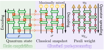
Figure 2: Protocol of classical shadow tomography for hybrid quantum circuits. The quantum state is efficiently encoded as classical information by randomized measurements in the data acquisition phase. A classical snapshot state is decoded by backward evolution from a maximally mixed state, given the circuit structure and measurement outcomes . On the other hand, its prior Pauli weights are inferred following the operator spreading dynamics.
Then following the assertion in Eq. (1), the classical snapshot associated with such measurement outcome should be identified as
(5)
where the denominator normalizes the classical snapshot as a state. Since the measurement circuit is composed of Clifford gates and Pauli measurements, every classical snapshot is a stabilizer state and can be efficiently represented and reconstructed on classical computers Gottesman (1997, 1998). As illustrated in Fig. 2, to reconstruct , one starts with a maximally mixed state (described by the density matrix ) and traces back the measurement circuit: inverting every unitary gate, replacing every measurement by projection to the measurement outcome, and normalizing the final state in the end.
Posterior and Prior Distributions. — We can interpret the hybrid quantum circuit measurement process as a measure-and-prepare quantum channel that measures the initial state and prepares the classical snapshot state with the posterior probability:
(6)
where denotes the probability of realizing a specific measurement circuit . Assuming that all Pauli measurements and Clifford gates are chosen uniformly, will only be affected by the measurement rate of the hybrid quantum circuit. By conducting the hybrid quantum circuit measurements of the target state repeatedly, one can sample classical snapshot states from the posterior distribution , forming an ensemble . The objective of classical shadow tomography is to predict properties of based on the samples of collected from experiments as classical data.
We introduce the prior distribution of the classical snapshot Akhtar et al. (2023), defined as . This distribution describes our knowledge about classical snapshots before observing the quantum state (as if is maximally mixed). The prior distribution solely characterizes the statistical properties of the randomized measurement scheme, reflecting our uncertainty about the measurement circuit structures and gate choices.
Pauli weight. — A crucial property of the prior classical snapshot ensemble is its Pauli weight Bu et al. (2022); Bertoni et al. (2022)
(7)
defined for any Pauli operator (where denotes the Pauli operator on the -th qubit). The Pauli weight fully characterizes the second-moment statistical feature of the prior distribution . It represents the probability for a Pauli observable to be transformed to the measurement basis and observed directly by the randomized measurement. It plays an important role in performing and analyzing classical shadow tomography.
For hybrid quantum circuits, the Pauli weight can be computed following the operator dynamics Ho and Abanin (2017); Bohrdt et al. (2017); Nahum et al. (2017); Kukuljan et al. (2017); von Keyserlingk et al. (2018); Nahum et al. (2018); Rakovszky et al. (2018); Khemani et al. (2018); Chan et al. (2018); Zhou and Chen (2019); Zhou and Nahum (2019); Xu and Swingle (2019); Chen and Zhou (2019); Parker et al. (2019); Qi et al. (2019); Kuo et al. (2020); Akhtar and You (2020). For every step of the physical evolution of a random quantum state through a random quantum channel , the Pauli weight will be updated by the Markov process 222See Appendix A for a brief review of the Markov evolution of Pauli weights.
(8)
where is the Pauli transfer matrix of the random channel ensemble . For every two-qubit random Clifford unitary channel and every probabilistic single-qubit random Pauli measurement channel , the corresponding Pauli transfer matrices are
(9)
where denotes the Kronecker delta symbol restricted to the support of the corresponding quantum channel. Starting from the initial Pauli weight of the maximally mixed state and applying the Pauli transfer matrix in accordance with the measurement circuit structure (see Fig. 2), the classical snapshot Pauli weight can be evaluated following Eq. (8) 333Strictly speaking, the classical snapshot Pauli weight dynamics is not Markovian due to the normalization factor on the denominator of Eq. (5). We are taking a Markovian approximation, that enables us to make thermodynamic-limit estimation of the shadow norm. The approximation is expected to work away from the measurement-induced critical point when the critical fluctuation is suppressed.. In the end, the Pauli weight should be normalized to to be consistent with the normalization of the classical snapshot states defined in Eq. (5).
Observable Estimation. — We now present a key result of our study: given any Pauli observable , its expectation value on the initial quantum state can be inferred from the posterior classical snapshots via Bu et al. (2022); Bertoni et al. (2022)
(10)
For more general observable , the expectation value can be similarly predicted by , where is the single-shot estimation Huang et al. (2020) of the observable given a particular classical snapshot , defined based on Eq. (10). This allows us to decode the quantum information about the original state from the classical shadows collected from the hybrid quantum circuit measurement. In practice, the expectation is often estimated by the median of means over a finite number of classical snapshots collected from experiments.
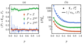
Figure 3: Demonstration of hybrid quantum circuit classical shadow tomography on a 12-qubit GHZ state. (a) Predicted observable expectation values and (b) locally-scrambled shadow norm as functions of the measurement rate . Colors label different Pauli observables .
To demonstrate the validity of Eq. (10), we carried out numerical experiments. We take the Greenberger-Horne-Zeilinger (GHZ) Greenberger et al. (2007) state of qubits, described by with . We consider a randomized measurement scheme implemented by shallow hybrid circuits, which contain three layers of random Clifford gates, together with random Pauli measurements inserted before each unitary layer with probability on each qubit. We simulate the protocol numerically on a classical computer by repeatedly preparing the GHZ state, applying the hybrid circuit, and collecting the measurement outcomes. For every given measurement rate , we collect samples and estimate the Pauli observables based on the measurement outcomes using Eq. (10). Our results, shown in Fig. 3(a), demonstrate that the estimated observable expectation values are consistent with their theoretical expectation on the GHZ state throughout the full range of , i.e., .
Sample Complexity Scaling. — The statistical uncertainty in the estimation, indicated by the error bar in Fig. 3(a), is due to the finite number of samples. The typical variance scales inversely with the number of samples. The coefficient is the locally-scrambled shadow norm, introduced in Ref. Hu et al. (2023). It upper-bounds the variance of the single-shot estimation over the prior classical snapshot ensemble . For Pauli observable , the shadow norm has a simple expression Bu et al. (2022); Bertoni et al. (2022)
(11)
In Fig. 3(b), the second moment of the single-shot estimation is compared with the inverse Pauli weight calculated from operator spreading dynamics. The results indicate a close match between the two measures. For generic observable , the shadow norm is given by . The shadow norm quantifies the number of samples needed to control the estimation variances below a desired level set by a small , which scales as . Therefore, the shadow norm measures the sample complexity for classical shadow tomography to predict the observable based on the randomized measurement scheme characterized by .
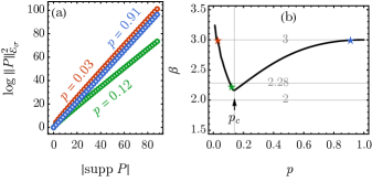
To study how the shadow norm scales with the operator size, we use the matrix product state (MPS) based approach developed in Ref. Akhtar et al. (2023); Bertoni et al. (2022) to compute the Pauli weight following the operator spreading dynamics and determine the shadow norm for consecutive Pauli string observables of different sizes . The result is plotted in Fig. 4(a). The shadow norm scales with the operator size exponentially with a base at the leading level
(12)
where stands for sub-leading correction that is polynomial in . This is consistent with the intuition that longer Pauli observable will require exponentially more local measurements to determine. However, the base depends on the measurement rate , as shown in Fig. 4(b).
Figure 4: (a) Dependence of log shadow norm of consecutive Pauli string observable of size at different measurement rates , demonstrating a leading linear behavior. (b) The base minimizes at a measurement rate that matches the measurement-induced transition of hybrid circuits. The measurement rates exemplified in (a) are highlighted as stars in (b).
We find that is minimized at when the hybrid quantum circuit operates at the measurement-induced criticality, and the shadow norm scales as
(13)
where and are determined by fitting. We expect the critical exponent to be universal, corresponding to the scaling dimension of a defect operator in the boundary conformal field theory (CFT) for the measurement-induced transition 444See Appendix B for a statistical mechanical model interpretation for the scaling behavior.. The minimal enters the region between and , which is the range of optimal scaling achievable by shallow circuit classical shadows Ippoliti et al. (2023).
The minimization of can be understood by examining it from both sides of the phase transition. In the area-law phase (), should decrease with decreasing measurement rate . This is because a lower measurement rate allows for a few more local measurements to be deferred to deeper layers of the unitary circuit, enabling larger-size observables to be probed more efficiently by leveraging the scrambling power of shallow circuits. However, in the volume-law phase (), if the measurement rate continues to decrease, will instead increase. Because the circuit’s scrambling power becomes so strong that it begins to hide the quantum information of the initial state from local measurements deep in the circuit Choi et al. (2020); Gullans and Huse (2020); Fan et al. (2021), which renders the measurements increasingly inefficient. As the measurement rate approaches zero (), the shadow norm must diverge, because it becomes impossible to reconstruct the initial state in the absence of measurements. Therefore, the optimal scaling of the shadow norm (or the sample complexity) can only occur at the transition point , where observables of all scales are probed efficiently 555See Appendix C for a more detailed quantitative analysis using toy models..
Summary and Discussions. — In this work, we present the classical shadow tomography approach for decoding quantum information from measurement outcomes of hybrid quantum circuits. This method involves computing classical snapshots associated with measurement outcomes and using them to infer properties of the initial quantum state. The Pauli weight of the prior classical snapshot ensemble characterizes the statistical properties of the randomized measurement scheme, and the shadow norm quantifies the sample complexity for predicting observables. The log shadow norm scales linearly with the operator size of the observable and exhibits optimal scaling at a critical measurement rate of the hybrid circuit that corresponds to the measurement-induced criticality.
Hybrid quantum circuits are known for their error correction encoding in the volume-law phase Choi et al. (2020); Gullans and Huse (2020); Fan et al. (2021). To use them as a random quantum error correction code, the ability to decode quantum information from measurement outcomes is essential. Classical shadow tomography provides a systematic and universal way to decode hybrid quantum circuits, making them suitable for more exciting quantum information applications.
Measurement-induced transition in hybrid quantum circuits was originally proposed as an entanglement transition. However, measuring entanglement entropy is a difficult task that requires post-selections. With classical shadow tomography, we can directly benchmark the prior classical snapshot Pauli weight on a known quantum states (assuming ),
(14)
where can be sampled by performing the hybrid circuit measurement on . Then can be extracted by fitting the dependence of with respect to its operator size . It is supposed to exhibit a kink at the measurement-induced transition as Fig. 4, which provides another method to detect the transition without post-selections apart from the cross-entropy benchmark Li et al. (2023).
Note added. — Up on finishing this work, we become aware that a related work Ippoliti and Khemani (2023) appeared.
Acknowledgements.
We acknowledge the helpful discussions with Ehud Altman, Matthew Fisher, Michael Gullans, Yaodong Li, and Bryan Clark. We are especially grateful to Ehud Altman for inspiring us on the quantum statistical mechanical model understanding of our results. A.A.A. and Y.Z.Y. are supported by a startup fund from UCSD. H.Y.H. is grateful for the support by Harvard Quantum Initiative Fellowship.
Bertoni et al. (2022)C. Bertoni, J. Haferkamp, M. Hinsche, M. Ioannou, J. Eisert,
and H. Pashayan, arXiv e-prints , arXiv:2209.12924 (2022), arXiv:2209.12924 [quant-ph] .
Note (2)See Appendix A for a brief
review of the Markov evolution of Pauli weights.
Note (3)Strictly speaking, the classical snapshot Pauli weight
dynamics is not Markovian due to the normalization factor on the denominator
of Eq. (5\@@italiccorr). We
are taking a Markovian approximation, that enables us to make
thermodynamic-limit estimation of the shadow norm. The approximation is
expected to work away from the measurement-induced critical point when the
critical fluctuation is suppressed.
A.1 Prior and Posterior Ensembles of Classical Snapshots
Assume the Krause operator (projection operator) describes a projective measurement implemented by a quantum circuit (with specific gate and observable choices) and resulted in the measurement outcomes , such that the probability to observe on a state is given by
(15)
If we have no knowledge about the state , we should assume to be maximally mixed, where stands for the identity operator in the Hilbert space and is effectively the Hilbert space dimension. In this
limit, Eq. (15) reduces to
(16)
The operator is a Hermitian and positive semi-definite operator, which motivates us to further normalize it to make it a state (a density matrix)
(17)
We will call a classical snapshot state. It has an important property that
(18)
Assume that the measurement circuit is drawn from some random ensemble with probability , we can define two random state ensembles for the classical snapshots:
•
the prior snapshot ensemble (with no knowledge about )
(19)
•
the posterior snapshot ensemble (given the knowledge about )
(20)
This means the ensemble averages are defined as
(21)
where stands for any function of , and are given by Eq. (16) and Eq. (15) respectively. Then Eq. (18) implies that the posterior ensemble average can be expressed as a prior ensemble average as
(22)
A.2 Review of Classical Shadow Tomography
Classical shadow tomography is an efficient approach to extracting information about an unknown quantum state by repeated randomized measurements. The idea of randomized measurement is to sample the measurement circuit (both its structure and its gate choices) from a probability distribution , perform the measurement on the state and collect the measurement outcomes . The randomized measurement effectively converts the quantum state into a collection of classical snapshots in the posterior ensemble .
The data acquisition procedure can be formulated as a quantum channel , called the measurement channel, which maps the initial quantum state to the expectation of classical snapshot states over the posterior snapshot ensemble
(23)
Here we have used Eq. (22). Suppose the randomized measurement scheme is topographically complete, the measurement channel will be invertible. Its inverse is called the reconstruction map, denoted as (albeit might not be a physical channel), such that the quantum state can be reconstructed from the classical snapshots by . This also provides the means to predict the expectation value of any observable on the state as
(24)
Note that due to the self-adjoint property of the measurement channel as well as the reconstruction map .
In practice, the expectation is often estimated by the median-of-means over a finite number of classical snapshots collected from experiments. Due to the statistical fluctuation of finite samples, the estimation value of an observable will fluctuate around its true expectation value with a typical variance that scales with the sample number as following the law of large numbers. The coefficient is the locally-scrambled shadow norm, defined as
(25)
By definition, the identity operator always have unit shadow norm, i.e., . For traceless observable , the locally-scrambled shadow norm quantifies the number of samples needed to control the estimation variances below a desired level set by a small , as . Therefore, the locally-scrambled shadow norm measures the sample complexity for classical shadow tomography to predict the observable based on the randomized measurement scheme characterized by .
A.3 Locally Scrambled Ensembles and Pauli Basis Approach
From the aforementioned general formulation, it is evident that the measurement channel and its inverse hold a central role in classical shadow tomography. Computing these for generic randomized measurement schemes is a complex task, and no polynomially scalable algorithm currently exists. Nevertheless, progress has been made in the context of locally scrambled (or Pauli-twirled) measurements, which are randomized measurements insensitive to local basis choices.
More specifically, let be a product of single-qubit unitary operators, decomposed as , with on every qubit . The product operator represents independent local basis transformations. Let be the unitary channel that implements the unitary transformation . A random state ensemble is said to be locally scrambled, if and only if for any . A random channel ensemble is considered locally scrambled, if and only if for any . A randomized measurement scheme is locally scrambled if its corresponding prior snapshot ensemble (as a random state ensemble) is locally scrambled. For locally scrambled randomized measurements, the associated and exhibit simple forms in the Pauli basis and can be computed efficiently. This conclusion remains valid when the scrambling condition is relaxed to , where denotes the single-qubit Clifford group, which is applicable to the cases of random Clifford gates with random Pauli measurements.
To elucidate this approach, it is more convenient to employ the Choi representation, wherein each quantum operator is viewed as a super-state :
(26)
where labels a complete set of orthonormal basis in the Hilbert space (of ket states). All Hermitian operators in span an operator space, denoted , in which inner product between two operators is defined as
(27)
Let represent a (multi-qubit) Pauli operator, constructed as a product of single-qubit Pauli operators, with acting on the th qubit. All Pauli operators form a complete set of orthonormal basis for the Hermitian operator space , as . Correspondingly, for any quantum channel that maps a state to another state , there exists a corresponding super-operator that maps their Choi representations accordingly, as .
Utilizing the Choi representation of quantum channel, any locally scrambled measurement channel defined in Eq. (23) can be written as a super-operator that acts on any state as
(28)
which indicates that . Expand in Pauli basis, we generally have
(29)
However, if we assume to be a locally scrambled state ensemble, the local scrambling property requires
(30)
Therefore, the measurement channel Eq. (29) becomes diagonal in the Pauli basis:
(31)
where denotes the average Pauli weight of classical snapshots in prior snapshot ensemble , defined as
(32)
This definition captures an essential statistical feature of the randomized measurement scheme: is the probability for the Pauli operator to appear diagonal in the measurement basis and be directly observed in a single random realization of the measurement protocol.
Since is diagonal in the Pauli basis, its inverse is simply given by
(33)
or, more explicitly, in terms of the reconstruction map on any operator as
(34)
Plugging Eq. (34) into Eq. (24) and Eq. (25) enables us to estimate the expectation value and study the shadow norm for any observable . In particular, for Pauli observable , we have
(35)
This essentially allows us to decode the quantum information in the initial state from the measurement outcomes gathered from a hybrid quantum circuit and to investigate the sample complexity for decoding various observables at different measurement rates.
A.4 Evolution of Pauli Weights through Locally Scrambled Channels
The central challenge now is to compute the average Pauli weight of the prior snapshot ensemble . In general, this remains a difficult problem. However, suppose the state ensemble is constructed by applying locally scrambled elementary quantum channels to locally scrambled simple initial states. In that case, its Pauli weight can be calculated using Markov dynamics, which is a more tractable approach.
To derive the dynamics of Pauli weights under locally scrambled quantum dynamics, we first introduce a set of region basis states in the doubled Hermitian operator space , defined by
(36)
where denotes a subset of qubits and denotes all Pauli operators supported exactly in region . is the cardinality of and denotes the number of qubits in . The significance of lies in its invariance under doubled local basis transformation, i.e., for any . In fact, all states form a complete set of orthonormal basis that spans the invariant subspace of under the doubled local scrambling .
Given a locally scrambled state ensemble and a locally scrambled channel ensemble , by definition, for any local basis transformation (or its corresponding unitary channel ), we have the following symmetry requirements
(37)
These manifest the locally scrambled properties on the 2nd-moment level. Given these symmetry requirements, the 2nd-moment locally scrambled random states (or channels) can and only need to be represented in the symmetric subspace spanned by the region basis as
(38)
where the linear combination coefficients and are defined as
(39)
which will be called the regional Pauli weights of the locally scrambled ensembles.
Locally scrambled quantum dynamics involve passing locally scrambled random states through locally scrambled random channels such that the resulting states still form a locally scrambled random state ensemble defined as:
(40)
Under such evolution, the 2nd-moment evolves as
(41)
By decomposing these 2nd-moment state and channel expectations in the region basis according to Eq. (38), we obtain the following evolution equation for the regional Pauli weights:
(42)
Suppose a locally scrambled state ensemble is obtained from random quantum dynamics comprised of locally scrambled simple channels, with computable regional Pauli weights. In that case, we can use Eq. (42) to trace the evolution of the regional Pauli weights of the state ensemble step-by-step, eventually inferring the regional Pauli weights of the final state ensemble. This approach enables us to systematically calculate the Pauli weights of the prior snapshot ensemble , which is the key for classical shadow tomography.
Finally, the regional Pauli weights and the ordinary Pauli weights are connected by the following relations, given and are Pauli operators supported on regions and , respectively,
(43)
Switching back to the Pauli basis, Eq. (42) reduces to a similar form
(44)
Based on these formulae, we can compute the Pauli weights for a few locally scrambled states and channels, which will be useful for analyzing the hybrid quantum circuit classical shadow tomography.
•
Locally scrambled state ensembles
–
Pure random product states
(45)
–
Pure Page state over qubits
(46)
–
Maximally mixed state
(47)
•
Locally scrambled channel ensembles
–
Local scrambling channel
(48)
–
Global scrambling channel among qubits
(49)
–
Local random projective measurement
(50)
A.5 Application to the Prior Snapshot Ensemble
According to Eq. (17), the classical snapshot state takes the form of
(51)
The state can be interpreted as mapping the maximal mixed state by a quantum channel , followed by a normalization,
(52)
where the quantum channel is defined by the Krause operator as . The random state ensemble of can be considered as derived from the random channel ensemble of ,
(53)
.
The maximally mixed state itself forms a locally scrambled state ensemble , whose Pauli weight is given by Eq. (47). Suppose the random channel ensemble is also locally scrambled, Eq. (44) can be applied to compute the Pauli weight of the composed state ensemble ,
However, what we wish to calculate is the Pauli weight of the classical snapshot ensemble, defined as
(56)
This ensemble average is difficult to calculate due to the potential correlation between its numerator and denominator. A common strategy is to approximate the average of ratios by the ratio of averages. Using Eq. (55), we have
(57)
Such that the Pauli weight of the classical snapshot ensemble can be approximately estimated as the ratio of two Pauli weights that we can compute by the operator dynamics Eq. (54). The approximation is expected to be asymptotically exact deep in both the volume-law and area-law phases where the correlated fluctuation between the numerator and denominator is suppressed. However, near the measurement-induced entanglement transition, the approximation will become inaccurate in estimating the location of the critical point and its universal properties. Nevertheless, it still provides an overall good picture of the behavior of the Pauli weight across the entanglement transition.
Appendix B Quantum Statistical Mechanical Picture
B.1 Pauli Weight and Entanglement Feature
Given the prior snapshot ensemble , we aim to compute the Pauli weight , which plays a central role in classical shadow tomography reconstruction and shadow norm estimation. The Pauli weight is defined as
(58)
for any Pauli operator and in qubit systems.
If is a locally scrambled ensemble, its 2nd moment if fully captured by the (2nd Rényi) entanglement feature, defined as
(59)
where denotes a subset of totally qubits in the system, which can also be encoded as a bit string such that the qubit marked by 1 belongs to the subset. denotes the swap operator in the region between the two replicas of . The Pauli weight and the entanglement feature are related by a linear transformation
(60)
where denotes the size (cardinality) of the set .
Figure 5: Statistical mechanical picture of the Pauli weight and the entanglement feature .
This relation can be simply expressed using the entanglement feature state, which is a fictitious quantum state that encodes the entanglement feature over all possible subsystems . Let be a set of orthonormal bit-string basis (i.e., assuming ), we can define the entanglement feature state for the ensemble as
(61)
then both the Pauli weight and the entanglement feature admits simple representation as
(62)
where the state is defined by
(63)
with being the all-0 state (the basis state of empty region ) and , are on-site operators in the entanglement feature Hilbert space. Physically, (or ) corresponds to the identity (or swap) boundary condition on the qubit in defining the 2nd-moment computation. The state defines the boundary condition for Pauli weight, corresponding to imposing the Pauli boundary condition within the Pauli operator support.
B.2 Entanglement Feature State in Measurement-Induced Transition
Suppose the prior snapshot state is given by with being the Kraus operator that describes a quantum channel of the hybrid quantum circuit with measurement rate .
•
limit, only contains a maximally mixed state, whose entanglement feature state is
(64)
where is the entanglement feature operator of the identity quantum channel, given by
(65)
•
limit, is an ensemble of random product state, meaning that the entanglement entropy vanishes for all regions, so , the entanglement feature state can be written as
(66)
where is the all-plus state with being the eigenstate of . Given that is also an eigenstate of , it does not hurt to rewrite
Eq. (66) as
(67)
Given the two limits Eq. (65) and Eq. (67), we can propose a variational ansatz for the entanglement feature state
(68)
where should interpolate between the ferromagnetic state and the paramagnetic state from to . A simple way to realize such an interpolation is to consider being the ground state of a transverse field Ising model
(69)
where the ratio is supposed to depend on the measurement rate in such a way that
(70)
Within this Ising model description, the measurement-induced entanglement transition happens at , corresponding to (at the Ising critical point). Although it should be emphasized that this is only a “mean-field” description of the entanglement transition, and it is known that the measurement-induced criticality is not in the Ising universality class. Nevertheless, this description provides us with ways to phenomenologically model and describe the Pauli weight for the prior snapshots of hybrid shadow tomography away from the critical point.
Given the variational ansatz of the entanglement feature state in Eq. (68), the Pauli weight can be evaluated as
(71)
where the denominator is introduced to normalize the Pauli weight (such that ) as the ansatz state was unnormalized. Introduce a binary indicator
At the limit, the entanglement feature state is given by Eq. (65), corresponding to as the ground state of the Ising model Eq. (69) at its ferromagnetic fixed point (). Given that is a product state, the Pauli weight Eq. (71) can be evaluated at each site independently,
(74)
The Pauli weight vanishes for all because without any measurement () there is no way to infer any information about any non-trivial Pauli observable.
To move away from this extreme limit, we can turn on the transverse field term in the Ising model Eq. (69) and use perturbation theory to estimate the corrected ground state in the regime. To the 1st order of , we have
(75)
where we exponentiate the leading order correction. With this, the Pauli weight becomes
(76)
Assuming is linear in , the above result implies that the shadow norm should scale with the Pauli operator size as
(77)
where is some unknown coefficient. So the base will diverge as as the measurement rate approaches zero, which is consistent with our numerical result in the main text.
B.4 Area-Law Phase ()
At the limit, the entanglement feature state is given by Eq. (67), corresponding to as the ground state of the Ising model Eq. (69) at is paramagnetic fixed point (). Given that is a project state, the Pauli weight Eq. (71) can be evaluated at each site independently,
(78)
given that . This reproduces the known result of Pauli weight for the random product state ensemble.
To move away from this extreme limit, we can turn on the Ising coupling in the Ising model Eq. (69) and use perturbation theory to estimate the corrected ground state in the regime. To the 1st order of , we have
(79)
With this, we can evaluate the inner product
(80)
where we have introduced the symbol
(81)
and exponentiate the perturbation (given ). Given the result Eq. (80), we can evaluate the Pauli weight using Eq. (73),
(82)
Assuming is linear in , the above result implies that the shadow norm should scale with the Pauli operator size as
(83)
where is some unknown coefficient. The base will decrease from as deviates from , which is also consistent with our numerical result in the main text.
B.5 Entanglement Transition ()
At , the hybrid quantum circuit undergoes measurement-induced entanglement transition. Although the transition is not described by the Ising CFT, it is instructive to gain a qualitative understanding about the transition using the Ising analogy. In the Ising analogy, the entanglement transition corresponds to the Ising critical point in the Ising model Eq. (69).
Suppose the ground state is now described by the Ising CFT. Using the Kramers-Wannier duality: , the string operator for a contiguous region can be mapped to the product of the dual Ising operator , such that
(84)
where corresponds to the scaling dimension of the dual Ising operator in the boundary CFT. Using this interpretation, we can expand
(85)
We can give a loose bound for the correlation by
(86)
therefore
(87)
Based on Eq. (71), the Pauli weight can be estimated by
(88)
which, given Eq. (84) and Eq. (87), can be bounded by
(89)
where is the size of the Pauli operator. Thus we conclude that the Pauli weight at should take the form of
(90)
with a base . Correspondingly, the shadow norm takes the form of
(91)
a form that is consistent with our numerical result in the main text. Our fitting in the main text shows that is within the bound.
B.6 Summary of Results
In conclusion, the quantum statistical mechanical model presented in this appendix shows that the shadow norm takes the following form
(92)
•
In the volume law phase, the base diverges as .
•
In the area law phase, the base approaches 3 from below as .
•
Given that increases in both phases as we go away from the critical point, the entanglement transition should have the minimal , denoted as , and (loosely) bounded by .
•
At the critical point, there is a power law correction , with universal exponent .
Appendix C Toy Models
C.1 Area-Law Phase ()
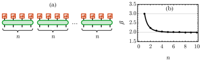
When the measurement rate is greater than the critical value , the classical snapshot is in the area-law phase. The measurement circuit can be modeled by Fig. 6(a), whose corresponding classical snapshot state is a product of -qubit random stabilizer state. Within each block, the entanglement is maximal. Between different blocks, there is no entanglement (product state). Therefore, the block size parameterizes the typical range of local entanglement in the classical snapshot state .
Figure 6: (a) A toy model for the randomized measurement in the area-law phase. Each green block represents a -qubit random Clifford gate. (b) The dependence of the shadow norm scaling base on the block size .
The limit corresponds to , that every qubit gets measured immediately before any inter-qubit scrambling. As the measurement rate reduces (but still in the area-law phase ), the system will be scrambled within the local entanglement range before gets probed by the measurement, but the scrambling range is still finite. This situation can be modeled by . We expect to increase effectively as we reduces from 1.
Consider a Pauli observable whose support happens to cover of the -qubit blocks. On one hand, the operator size of is . On the other hand, its Pauli weight is given by
(93)
This result can be understood as follows. The Pauli weight can be interpreted as the probability that a Pauli observable gets transformed by the random Clifford gates into a diagonal operator in the measurement basis, such that it can be directly probed by the measurement. Within each -qubit block, the random Clifford gate scrambles any particular non-identity Pauli observable to one of all non-identity Pauli observables, among which only are diagonal (as Pauli strings of and ) in the measurement basis. Hence the probability of to be diagonalized within each block is . To diagonalize across all the blocks, the probability multiplies to , as concluded in Eq. (93). As a result, the shadow norm of is
(94)
Assuming the shadow norm scales with the operator size as , the base can be extracted as
(95)
The dependence of on is shown in Fig. 6(b). As the measurement rate decreases from 1, the scrambling range increases, and will eventually decrease from to (in this toy model’s ideal case).
C.2 Volume-Law Phase ()
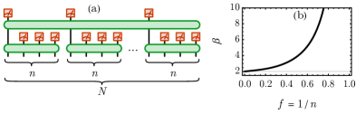
When the measurement rate is less than the critical value , the classical snapshot is in the volume-law phase with local error correction encoding. A model to describe such states is to consider random stabilizer states further encoded by random stabilizer codes. The corresponding measurement circuit will be like Fig. 7(a). The system contains physical qubits, grouped by -qubit blocks. Within each block, the physical qubit is first decoded into a logical qubit and syndrome qubits. The syndrome qubits are measured, and the logical qubits are further scrambled before being finally measured. We assume .
Figure 7: (a) A toy model for the randomized measurement in the volume-law phase. Each green block represents a random Clifford gate. The lower layer gates serve as the encoding gates of random stabilizer codes in each -qubit block. The upper layer gate scrambles all the logical bits. (b) The dependence of the shadow norm scaling base on the volume-law coefficient .
Consider an entanglement region that covers exactly of the -qubit blocks (assuming ), the entanglement entropy of in such region scales as , while the region size is . So is a volume-law state with the volume-law coefficient
(96)
This ratio is also the rate of the local error correction code (the ratio between the numbers of logical v.s. physical qubits). As the measurement rate increases from 0 to , the volume-law coefficient decreases from 1 to 0, corresponding to increasing from 1 to .
Consider a Pauli observable whose support happens to cover of the -qubit blocks. On one hand, the operator size of is . On the other hand, its Pauli weight is given by
(97)
This result can be understood as follows. The Pauli weight can be interpreted as the probability that a Pauli observable gets transformed by the random Clifford gates into a diagonal operator in the measurement basis, such that it can be directly probed by the measurement. There are two possible scenarios:
•
gets transformed to an operator that is non-identity and diagonal in the syndrome subspace and identity in the logical subspace. The probability for this to happen is . Because in each block, any particular non-identity Pauli observable will be transformed to one of the non-identity Pauli observable, among which only are syndrome subspace diagonal and logical subspace identity. They are of the following form:
(98)
So the probability for this to happen is in each block and over blocks. In this case, will be directly measured by the syndrome qubit measurements. After the measurement, it collapses to an identity operator on logical qubits, whose measurement outcome can be determined with probability 1. Therefore, this scenario has a total contribution of to the Pauli weight, corresponding to the first term in Eq. (97).
•
gets transformed to an operator that is non-identity and diagonal in both the syndrome and logical subspaces. The probability for this to happen is . Within each block, any particular non-identity Pauli observable will be transformed to one of the non-identity Pauli observables, among which only are diagonal in the syndrome subspace regardless of its action in the logical subspace. They are of the following form
(99)
So the probability for this to happen is and over blocks. After the syndrome qubit measurements, the operator will collapse to a Pauli string in the logical subspace of the following form
(100)
This has not excluded the possibility of , which should be excluded to avoid double counting the same scenario discussed previously. Thankfully, we already know that the probability for to become a logical identity operator after the syndrome qubit measurement is . So the probability for to be syndrome diagonal and logical non-identity is . Under the global scrambling of logical qubits by the upper layer gate, the observable gets further mapped to one of the non-identity Pauli operators in the logical subspace, among which only are diagonal and can be directly probed by the logical qubit measurements. So this further multiplies the probability by , resulting in a contribution of to the Pauli weight, corresponding to the second term in Eq. (97).
According to Eq. (97), in the thermodynamic limit , so the second term can be neglected, and the Pauli weight is dominated by the first term
(101)
In conclusion, the shadow norm of in this toy model is given by
(102)
Assuming the shadow norm scales with the operator size as , the base can be extracted as
(103)
Given that is related to the volume law coefficient by Eq. (96), the base can also be expressed in terms of as
(104)
The dependence of on is shown in Fig. 7(b). As the measurement strength increases from to , the volume-law coefficient decreases from to , and decreases from to . Near the measurement induced phase transition (as ), increases with the volume-law coefficient as .