MARLIM: Multi-Agent Reinforcement Learning
for Inventory Management

Abstract

Maintaining a balance between the supply and demand of products by optimizing replenishment decisions is one of the most important challenges in the supply chain industry. This paper presents a novel reinforcement learning framework called MARLIM, to address the inventory management problem for a single-echelon multi-products supply chain with stochastic demands and lead-times. Within this context, controllers are developed through single or multiple agents in a cooperative setting. Numerical experiments on real data demonstrate the benefits of reinforcement learning methods over traditional baselines.

1 Introduction

Inventory control [49] is one of the major problems in the supply chain industry. The main goal is to ensure the right balance between the supply and demand of products by optimizing replenishment decisions. More precisely, a controller observes the past demands and local information of the inventory and has to decide about the next ordering values. Accurate inventory management is key to running a successful product business with benefits ranging from better inventory accuracy and insights to cost savings and avoidance of shortage and stock overflows.

The main issue of the supply chain is the environment uncertainty [64]. In an ideal world with deterministic demand and lead-times, an inventory controller would be able to place a perfect order equal to the demand size at the right time. However, in practice, both the demands and lead-times are stochastic with potentially high volatility, making the inventory management problem hard to solve. In most cases, the inventory controller may exceedingly or insufficiently order. The former case leads to paying unnecessary ordering and holding costs while the latter results in shortage costs which may jeopardize the company’s performance.

Classical methods for solving the inventory management problem rely on basic heuristics [63, 55] due to the complexity of the mathematical modeling of the inventory system. While these approaches are easy to implement, they are not able to capture the randomness of the demand and lead-times. Another way of solving the inventory management problem is dynamic programming [5]. Despite being efficient, this technique requires exact knowledge of the mathematical model of the inventory system, which becomes intractable for big companies with very large inventories. Inventory management models can quickly become too complex and time-consuming, leading to unworkable models [22]. To escape this curse of dimensionality, one may apply approximate dynamic programming [23, 17] which performs well in specific settings at the cost of strong assumptions and simplifications.

Since the environment uncertainty is the major problem of inventory control [12], reinforcement learning (RL) methods appear as a natural solution since they can model complex situations and generalize well in a data-driven manner. The reinforcement learning task [53] consists, for an autonomous agent (e.g., a robot), in learning the actions to be taken, from trials, in order to optimize a quantitative signal over time. Such paradigm has reached tremendous success in games [35, 48, 56], but the early applications of reinforcement learning to real-world tasks, e.g., robotics [29] or autonomous driving [37, 45] remain a challenge and an active field of research. Furthermore, most of the literature on inventory management systems is meant to be applied for companies which are specialized in the retail industry where (i) the items of the inventory are meant to be sold and (ii) item shortages may be addressed through back orders. However, many companies are interested in inventory management for factories and warehouses where the objective is to ensure the performance of a production line and avoid the drastic consequences of item shortages.

The main goal of this paper is to develop a novel reinforcement learning framework, called MARLIM, to address the inventory management problem for a single-echelon multi-products supply chain on a production line with stochastic demands and lead-times.

Related work. The stochastic inventory control problem is one of the most studied problems in inventory theory. It was initiated by the seminal works of [20] and [49] which presented the basic heuristics to solve the inventory management problem. The so-called (s,S) policy [63], which results from the economies of scale in procurement, is a widely used policy nowadays in practice. However such heuristic cannot capture the randomness of the demand and lead-times, making it difficult to apply to realistic use cases. Later on, several authors developed the theory of inventory management and one may refer to the books of [64, 40] and [32] for an in-depth coverage of the topic. The different state-of-the-art models for inventory management systems may be found in the recent survey of [12].

In the past few years, many comprehensive studies related to the integration of reinforcement learning techniques to the inventory management problem were presented, starting with the work of [21] which considered production and distribution functions of global supply chain with multiple stages assuming a single item. Later on, different variations were derived with a particular focus on a supply chain with two echelons [28, 31], multiple echelons [27, 30, 11, 52] or multiple retailers [25, 16]. In all these studies, reinforcement learning methods have been implemented to specify near-optimal ordering policies in the entire supply chain with different goals such as maximizing the profit (when considering retailers) or minimizing costs composed of either ordering and holding costs or holding and backorder costs but not all of them at the same time. Furthermore, all the mentioned studies are dealing with a simplified assumption of independent products with no interactions among them.

In order to handle multiple items and accurately model the inter-dependency between them, the proposed framework of this paper is based on the multi-agent reinforcement learning paradigm [36] where each item may be seen as a single agent. Such framework seems promising to improve the training efficiency as suggested by the recent survey of [61] and the two recent studies of multi-agent reinforcement learning applied to inventory management problems [2, 51]. In [2], the authors derive a reinforcement strategy for a grocery retailer with multiple items and fixed delivery times where the focus is on the items availability rather than their associated costs. Similarly the study of [51] deals with a multiple echelons supply chain with predefined lead times whose aim is to maximise product sales and minimise wastage of perishable products. Conversely, the developed method of this paper is focused on the reduction of operating costs on a production line with stochastic demands and lead-times for real-world applications.

The framework of MARLIM is also related to the joint replenishment problem, i.e., when one considers the interdependency among different groups of products in a same order provided by a single supplier [26, 57, 44]. The objective is to optimize a global replenishment cost composed of inventory ordering and holding costs [42, 58] but does not take into account the losses induced by item shortages. In contrast to these previous studies, the aim of the proposed method whose is not only to reduce the global replenishment cost but also to avoid stock-outs of items.

Contributions. The main contributions of this paper may be summarized as follows.
• A novel reinforcement learning framework, called MARLIM, is developed to address the inventory management problem for a single-echelon multi-products supply chain on a production line with stochastic demands and lead-times.
• A methodology to train agents in different scenarios for fixed or shared capacity constraints with specific handling of storage overflows is provided.
•  Various numerical experiments on real-world data demonstrate the benefits of the developed method over classical baselines.

Outline. Section 2 presents the mathematical background of reinforcement learning and Section 3 deals with the inventory management model. The methodology and details of the developed supply chain environment are described in Section 4. Numerical experiments are performed in Section 5 to highlight the relevance of the developed model on real-world data and Section 6 concludes the article with further discussion.

2 Preliminaries on Reinforcement Learning

Markovian setting. Markov Decision Processes (MDP) [41] are a formalization of sequential decision making, where actions influence not just immediate rewards, but also subsequent situations. Consider the classical framework of a MDP defined as a tuple $\mathcal{M}=\langle\mathcal{S},\mathcal{A},p,r,\gamma,\mu\rangle,$ comprised of a state space $\mathcal{S},$ an action space $\mathcal{A},$ a Markovian transition kernel $p:\mathcal{S}\times\mathcal{A}\rightarrow\Delta(\mathcal{S})$ where $\Delta(\mathcal{S})$ denotes the set of probability density functions over $\mathcal{S},$ a reward function $r:\mathcal{S}\times\mathcal{A}\rightarrow\mathbb{R},$ a discount factor $\gamma\in(0,1)$ and an initial-state distribution $\mu\in\Delta(\mathcal{S})$. The reinforcement learning problem consists of finding the best strategy or policy $\pi:\mathcal{S}\to\mathcal{A}$ in order to maximize the performance. The criterion here is defined in terms of future rewards that can be expected and depend on the agent’s behavior. The solution of a MDP is an optimal policy $\pi^{*}$ that maximizes the value function $V^{\pi}$ in all the states $s\in\mathcal{S}$ over some policy set of interest $\Pi$: $\pi^{\star}\in\operatorname*{argmax}_{\pi\in\Pi}V^{\pi}$. Such optimal policy $\pi^{\star}$ is guaranteed to exist thanks to the theorem of [6]. In practice, $\pi^{\star}$ can be found through dynamic programming and Bellman equations [7, 9, 24] with different schemes, e.g., policy iteration [8, 10] or value iteration [39, 50]. Another way is to consider policy-gradient methods [60, 4] which use a parameterized policy $\pi_{\theta}$ with $\theta\in\Theta\subset\mathbb{R}^{d}$ and update the policy parameter $\theta$ on each step in the direction of an estimate of the gradient of the performance with respect to the policy parameter.

Parametric policies. Given a parameter space $\Theta\subseteq\mathbb{R}^{d}$, consider a class of smoothly parameterized stochastic policies $\Pi_{\Theta}=\left\{\pi_{\theta},\theta\in\Theta\right\}$ that are twice differentiable w.r.t. $\theta$, i.e., for which the gradient $\nabla_{\theta}\pi$ and the Hessian $\nabla_{\theta}^{2}\pi_{\theta}$ are defined everywhere and finite. When the action space is finite, a popular choice is to use Gibbs policies, a.k.a. softmax policies, for all $s\in\mathcal{S}$ and $a\in\mathcal{A}$,

$$\pi_{\theta}(a|s)=\frac{\exp(\theta^{T}\psi(s,a))}{\sum_{a^{\prime}\in\mathcal{A}}\exp(\theta^{T}\psi(s,a^{\prime}))}$$ (1)

where $\psi:\mathcal{S}\times\mathcal{A}\rightarrow\mathbb{R}^{d}$ is an appropriate feature-extraction function, often computed using a neural network. When the action space is continuous $\mathcal{S}\subset\mathbb{R}^{d}$, a popular choice is to use Gaussian policies so the policy can be defined as the normal probability density over a real-valued scalar action, with some parametric mean $\mu:\Theta\times\mathcal{S}\rightarrow\mathbb{R}$ and standard deviation $\sigma:\Theta\times\mathcal{S}\rightarrow\mathbb{R}_{+}$ that depend on the state, for all $s\in\mathcal{S}$ and $a\in\mathcal{A}$,

$$\pi_{\theta}(a|s)=\frac{1}{\sigma_{\theta}(s)\sqrt{2\pi}}\exp\left(-\frac{(a-\mu_{\theta}(s))^{2}}{2\sigma_{\theta}(s)^{2}}\right).$$ (2)

Multi-Agent Reinforcement Learning (MARL). Originated from the seminal works of [47] and [34], Markov Games are the standard generalization of Markov Decision Processes as they capture the interaction of multiple agents. A Markov game is defined as a tuple $\langle\mathcal{N},\mathcal{S},(\mathcal{A}^{i})_{i\in\mathcal{N}},p,(r^{i})_{i\in\mathcal{N}},\gamma\rangle$ where $\mathcal{N}$ denotes the set of agents, $\mathcal{S}$ is the state space observed by all agents, $\mathcal{A}^{i}$ is the action space of agent $i$. $\mathcal{A}=\prod_{i\in\mathcal{N}}\mathcal{A}^{i}$ denotes the joint action space, $p:\mathcal{S}\times\mathcal{A}\to\Delta(\mathcal{S})$ is the transition kernel, $r^{i}:\mathcal{S}\times\mathcal{A}\rightarrow\mathbb{R}$ is the immediate reward function of agent $i$ and $\gamma\in(0,1)$ is the discount factor. At time step $t$, each agent $i\in\mathcal{N}$ selects an action $a_{t}^{(i)}$ based on the system state $s_{t}$. The system then transitions to state $s_{t+1}$ according to $p$ and rewards each agent $i$ with $r^{i}(s_{t},a_{t})$. The goal of agent $i$ is to optimize its own long-term reward by finding the policy $\pi^{(i)}:\mathcal{S}\to\Delta(\mathcal{A}^{i})$ such that $a_{t}^{(i)}\sim\pi^{(i)}(\cdot|s_{t})$. Therefore, the marginal value function $V^{(i)}:\mathcal{S}\to\mathbb{R}$ of agent $i$ becomes a function of the joint policy $\pi:\mathcal{S}\to\mathcal{A}$ defined by $\pi(a|s)=\prod_{i\in\mathcal{N}}\pi^{(i)}(a^{(i)}|s),V^{(i)}(s)=\mathbb{E}\left[\sum_{t\geq 0}\gamma^{t}r^{i}(s_{t},a_{t})\Big{\rvert}a_{t}^{(i)}\sim\pi^{(i)}(\cdot|s_{t}),s_{0}=s\right].$ Thus, the solution concept of a Markov game deviates from that of a MDP since the optimal performance of each agent is controlled not only by its own policy, but also the choices of all other players of the game. The most common solution concept for Markov games is Nash equilibrium [3, 18].

As a standard learning goal for MARL, Nash equilibrium always exists for finite-space infinite-horizon discounted Markov games [18], but may not be unique in general. Most of the multi-agent reinforcement learning algorithms are contrived to converge to such an equilibrium point, if it exists.

3 Inventory Management Model

Denote by $\mathcal{N}=\{1,\ldots,n\}$ the discrete product space where $i\in\mathcal{N}$ refers to the $i^{th}$ item in the inventory and $n$ is the total number of items. At each time step, the inventory controller decides about the order to take based on the current inventory level and the previous demands. This order arrives in the inventory after a stochastic lead-time. After receiving the replenishment quantity of different products, the demands are satisfied and the environment incurs inventory costs. The aim of this Section is to describe the complete inventory management model from the inventory features and inventory costs to the inventory dynamics of the system.

3.1 Inventory features

The different inventory features are the basis of the inventory management model as they model the state space and the dynamics of the underlying Markov game. The inventory level $x_{t}\in\mathbb{R}^{n}$ is the on-hand inventory at time $t$, i.e., the quantity of products sitting on the shelf in the inventory. At each time step, the inventory controller receives a stochastic demand signal $\delta_{t}\in\mathbb{R}^{n}$ and can order a quantity $a_{t}\in\mathbb{R}^{n}$ of items. These quantities arrive in the inventory after some lead-time $\tau_{t}\in\mathbb{R}^{n}$. The inventory replenishment quantity $\rho_{t}\in\mathbb{R}^{n}$ is the associated quantity of products which is on its way to the inventory, i.e., it is the quantity that will be added to the inventory level when the inventory check is done at the next time step.

Symbol	Feature
$\Lambda^{(k)}$	maximum capacity of subspace $k$
$x_{t}^{(i)}$	inventory level of product $i$ at time $t$
$a_{t}^{(i)}$	order of product $i$ at time $t$
$\rho_{t}^{(i)}$	replenishment of product $i$ at time $t$
$\lambda_{t}^{(i)}$	temporary level of product $i$ at time $t$
$w_{t}^{(i)}$	overflow weight of product $i$ at time $t$
$\Omega_{t,k}^{\phantom{()}}$	stock overflow of subspace $k$ at time $t$
$\delta_{t}^{(i)}$	demand of product $i$ at time $t$
$\tau_{t}^{(i)}$	lead-time of product $i$ at time $t$
$\beta_{t}^{(i)}$	backlog of product $i$ at time $t$
$C_{o}^{(i)}$	Ordering cost of product $i$
$C_{h}^{(i)}$	Holding  cost of product $i$
$C_{s}^{(i)}$	Shortage cost of product $i$

When receiving the replenishment quantity, the inventory levels are temporarily updated through $\lambda_{t}\in\mathbb{R}^{n}$ and some storage overflow may happen. When this overflow event happens, denoted by $\Omega_{t}$, the replenishment quantities are scaled using weights $w_{t}\in\mathbb{R}^{n}$ to ensure that the total inventory level does not exceed the maximum storage capacity $\Lambda\in\mathbb{N}^{+}$. Finally, the demands are satisfied and the controller updates the inventory levels $x_{t+1}$. When demand exceeds the available inventory level for an item, it yields a shortage cost computed through a backlog level $\beta_{t+1}\in\mathbb{R}^{n}$. When optimizing the decisions relative to the inventory, the controller must take into account the different inventory costs.

3.2 Inventory costs

The inventory costs may be classified into three categories [55]: ordering, holding and shortage.

(i) Ordering costs: in the case of an ordering setting, these costs include the functioning costs, reception and tests costs, the salaries of the personnel, information systems costs and customs costs. In the case of a production setting, these costs include the raw material costs, labor costs, fixed and variable overheads, e.g., rent of a factory or the energy consumption allocated for production.

(ii) Holding costs: these are associated with storing inventory that remains unused and may be divided into two categories: financial and functional costs. The former represent the financial interest of the money invested in procuring the stocked products. The latter include the rent and maintenance of the required space, insurance costs, equipment costs, inter-warehouses transportation and obsolescence costs.

(iii) Shortage costs: when demand exceeds the available inventory for an item. The related costs fall in one of the two following categories: lost sales costs and backlogging costs. When considering lost sales, the unsatisfied demands are completely lost whereas with backlogging costs, there is a penalty shortage cost. Note that in the case where the stock is internal, the inventory shortage will induce the stop of production of therefore all the consequent costs.

For any item $i\in\mathcal{N}$, denote by $C_{o}^{(i)},C_{h}^{(i)}$ and $C_{s}^{(i)}$ the unit ordering, holding and shortage costs respectively. The different features of the inventory management system are summarized in the Table above.

Remark 1

(Costs and priority) The different unit costs are the keystone to accurately model different behaviors among the items. Intuitively, items with high shortage cost correspond to critical items that should not run out-of-stock. On the contrary, items with high ordering cost should be ordered sparingly. In general, an optimal controller should consider some reward function which leverages these three factors to find the right balance between the different costs.

3.3 Inventory Dynamics

The different relations between the inventory features are the mainstay to model a Markov game. First of all, there is a capacity constraint on the storage space and several structures are to be considered. On the one hand, a natural assumption is to consider that each item $i\in\mathcal{N}$ has a maximum capacity $\Lambda^{(i)}\in\mathbb{N}^{\star}$. In practice, thanks to expert’s knowledge, an estimate of the mean demand of each item may be available so that the capacity of each product can be upper bounded. On the other hand, for economical reasons, the total storage space may be shared among all items. This model allows more flexibility as products can compete for storage space but it assumes that all items belong to a same category. A unified and more realistic setting is the following: the different products may be classified into different types and they only compete for storage space inside their category (see Remark 2). In other words, the product space $\mathcal{N}$ can be decomposed into $K$ different clusters of products, i.e.,

$$\mathcal{N}=\bigcup_{k=1}^{K}\mathcal{N}_{k}.$$

Each product subspace $\mathcal{N}_{k}$ has a maximum storage capacity $\Lambda^{(k)}\in\mathbb{N}^{\star}$. For the sake of clarity, all items are assumed to have the same volume (see Remark 3). At each time step $t\geq 0$, the available storage space of each product subspace should be non-negative, i.e., for all $k=1,\ldots,K$

$$\Delta_{t}^{(k)}=\Lambda^{(k)}-\left(\sum_{i\in\mathcal{N}_{k}}x_{t}^{(i)}\right)\geq 0.$$ (3)

The replenishment quantity $\rho_{t}$ depends on the previous orders $a_{1},\ldots,a_{t}$ and their associated lead-times. Indeed, the received quantity of product $i$ at time $t$ corresponds to all the previous orders $a_{j}^{(i)}$ made at time step $j$ such that the receiving time $(j+\tau_{j})$ obtained by adding the associated lead-time matches the current time step $t$, i.e., for $i=1,\ldots,n$,

$$\rho_{t}^{(i)} =\sum_{j=1}^{t}a_{j}^{(i)}\mathds{1}_{\{j+\tau_{j}^{(i)}=t\}}.$$

When receiving these replenishment quantities at time $t$, the inventory levels are temporarily updated as $\lambda_{t}^{(i)}=x_{t}^{(i)}+\rho_{t}^{(i)}$ and it may happen that the storage space of subspace $\mathcal{N}_{k}$ overflows which translates into the following event

$$\Omega_{t,k}=\left\{\sum_{i\in\mathcal{N}_{k}}\lambda_{t}^{(i)}>\Lambda^{(k)}\right\}.$$

In virtue of Eq.(3), on $\Omega_{t,k}$ it holds $\sum_{i\in\mathcal{N}_{k}}\rho_{t}^{(i)}>\Delta_{t}^{(k)}$. This means that when the stock overflow happens in $\mathcal{N}_{k}$ then the received replenishment quantities of products in $\mathcal{N}_{k}$ exceed the available storage space of $\mathcal{N}_{k}$. In that case, the replenishment quantities are weighted to completely fill the available storage space, i.e., some overflow weights $w_{t}^{(i)}$ are chosen such that $\sum_{i\in\mathcal{N}_{k}}w_{t}^{(i)}\rho_{t}^{(i)}=\Delta_{t}^{(k)}$. In order to promote the replenishment of critical products (see Remark 4), the overflow weights are set to be proportional to the shortage cost of items. For all $k=1,\ldots,K$ and $i\in\mathcal{N}_{k}$,

$$w_{t}^{(i)} =\mathds{1}_{\Omega_{t,k}^{\phantom{c}}}\left(\frac{\Delta_{t}^{(k)}C_{s}^{(i)}}{\sum_{j\in\mathcal{N}_{k}}C_{s}^{(j)}\rho_{t}^{(j)}}\right)+\mathds{1}_{\Omega_{t,k}^{c}}.$$ (4)

Since the quantities of products are non-negative integers, only the integer part of the weighted replenishment quantities $w_{t}\rho_{t}$ are added to the current inventory levels $x_{t}$. When the demands exceed the available on-hand inventory levels, a backlog is computed to monitor the unmet demands and measure the associated shortage costs.

For each item $i\in\mathcal{N}$, the inventory level and backlog are updated as

$$x_{t+1}^{(i)}=\left(x_{t}^{(i)}+\lfloor w_{t}^{(i)}\rho_{t}^{(i)}\rfloor-\delta_{t}^{(i)}\right)_{+},\quad\beta_{t+1}^{(i)}=\beta_{t}^{(i)}+\left(x_{t}^{(i)}+\lfloor w_{t}^{(i)}\rho_{t}^{(i)}\rfloor-\delta_{t}^{(i)}\right)_{-}$$

where $(\cdot)_{+}=\max(\cdot,0)$ and $(\cdot)_{-}=\max(-\cdot,0)$ denote the positive and negative parts respectively. The inventory dynamics is summarized in Figure LABEL:fig:inventory_dynamics above.

Remark 2

(Product clusters) In practice, the different items of a warehouse are naturally classified into several groups according to their storage conditions: size, weight and specific climatic conditions, e.g., temperature, pressure, humidity levels, ventilation and light.

Remark 3

(Storage capacity) In the case where the total storage space is shared among all items ($K=1$), the capacity constraint is fulfilled as soon as $x_{t}^{T}\mathds{1}_{n}\leq\Lambda$ where $\Lambda$ is the maximum capacity of the warehouse. To model different volumes of items, one can simply consider a vector of unit volumes $v\in\mathbb{R}^{n}$ where $v^{(i)}$ is the unit volume of product $i$ and ensures that $x_{t}^{T}v\leq\Lambda$ for all $t\geq 0$. Similarly, when dealing with $K$ types of products, the capacity constraint of each subspace $\mathcal{N}_{k}$ becomes $\sum_{i\in\mathcal{N}_{k}}x_{t}^{(i)}v^{(i)}\leq\Lambda^{(k)}$ for all $t\geq 0$.

Remark 4

(Storage overflow) Different options are available to address the storage overflow of a product subspace $\mathcal{N}_{k}$. If all items in $\mathcal{N}_{k}$ have equal priority levels, one could think of a uniform split of the available storage space of the form $\Delta_{t}^{(k)}/|\mathcal{N}_{k}|$. However, in practice, some items are more important than others and may even be critical for production. This is why, when the storage space overflows, the replenishment quantities should be weighted to favor the replenishment of products non only with low inventory levels but also the ones associated to large shortage costs (see Eq.(4))

4 MARL for Inventory Management

Recall that the goal of any MARL algorithm is to find a policy $\pi_{\theta}$ maximizing the expected discounted reward $V(\pi_{\theta})=\mathbb{E}\left[\sum_{t\geq 0}\gamma^{t}r(s_{t},a_{t})|a_{t}\sim\pi_{\theta}\right].$ The goal of this Section is to derive the necessary formalism, namely the Markov games and associated rewards, in order to apply such MARL methods.

Markov games. The inventory management problem can be modeled as $K$ different Markov games. Consider a fixed product subspace $\mathcal{N}_{k}$ with $1\leq k\leq K$. At time step $t\geq 0$, the state of agent $i\in\mathcal{N}_{k}$ is comprised of: the inventory level $x_{t}^{(i)}$, the replenishment quantity $\rho_{t}^{(i)}$, the lead time $\tau_{t}^{(i)}$ and backlogs $\beta_{t}^{(i)}$, i.e., $s_{t}^{(i)}=(x_{t}^{(i)},\rho_{t}^{(i)},\tau_{t}^{(i)},\beta_{t}^{(i)})\in\mathcal{S}_{k}^{i}$. The action of each agent concerns the ordering quantity $a_{t}^{(i)}\in\mathcal{A}_{k}^{i}=\llbracket 0,\Lambda^{(k)}\rrbracket$. The joint state space and action space are respectively given by $\mathcal{S}_{k}=\prod_{i\in\mathcal{N}_{k}}S_{k}^{i}$ and $\mathcal{A}_{k}=\prod_{i\in\mathcal{N}_{k}}\mathcal{A}_{k}^{i}$. The transition kernel is implicitly defined by all the inventory dynamics equations of Section 3.3.

Costs and rewards. According to Section 3.2, at each time step $t\geq 0$ and for a given product subspace $\mathcal{N}_{k}$, each agent $i\in\mathcal{N}_{k}$ incurs some inventory costs $C_{t}^{(i)}$ given by the combination of ordering, holding and shortage costs. In other words, the overall inventory cost may be described as

$$C_{t}^{(i)}=\alpha_{o}\underbrace{a_{t}^{(i)}C_{o}^{(i)}}_{\text{ordering}}+\alpha_{h}\underbrace{x_{t}^{(i)}C_{h}^{(i)}}_{\text{holding}}+\alpha_{s}\underbrace{\beta_{t+1}^{(i)}C_{s}^{(i)}}_{\text{shortage}}$$

where $\alpha_{o},\alpha_{h},\alpha_{s}\in[0,1]$ with $\alpha_{o}+\alpha_{h}+\alpha_{s}=1$ are weighting coefficients that translate some expert’s knowledge about the desired strategy. This expression translates the trade-off between the different inventory costs. Hopefully, a trained agent will learn to order low quantities of products that are costly to stock and supply, while maintaining sufficient inventory levels to avoid stock-outs for critical products associated to large shortage costs. This is validated in the numerical experiments of Section 5.

The inventory costs of each agent are associated to the single reward defined as: $r^{i}(s_{t},a_{t})=-C_{t}^{i}$. Observe that inside a product subspace $\mathcal{N}_{k}$, the agents are working in a cooperative setting in order to optimize the average reward corresponding to $r_{k}(s_{t},a_{t})=\sum_{i\in\mathcal{N}_{k}}r^{i}(s_{t},a_{t})/|\mathcal{N}_{k}|$. This average reward model allows more heterogeneity among agents and facilitates the development of decentralized MARL algorithms [62, 15]. More subtly, the reward function is sometimes not sharable with others, as the preference may be private to each agent. Note that this setting finds broad applications in engineering systems as sensor networks [43], smart grid [14], intelligent transportation systems [1], and robotics [13].

5 Numerical Experiments

This Section is dedicated to numerical experiments on real data. Various scenarios regarding the capacity constraints of the warehouses are considered: (i) when the items in a product cluster have their own capacity constraints then it is enough to train a single RL agent and apply the resulting behavior to all the items in that cluster; (ii) when the items compete for storage space then one may apply some MARL algorithm to deal with the interdependency of items.

Stochastic Model. The demands and lead-times are assumed to be stochastic with stationary distributions. The lead-times follow geometric distributions and the demands follow a mixed law of Poisson process with zero plateaus. More precisely, for each item $i$, the lead-time is given by $\tau^{(i)}\sim\mathcal{G}(p_{i})$ with parameter $p_{i}\in(0,1)$ and the demand distribution is given by

$$\delta^{(i)}=\left\{\begin{array}[]{ll}\mathcal{P}(\mu_{i})&\text{with probability }b_{i}\\ 0&\text{with probability }1-b_{i}\end{array}\right.$$

In other words, the demand process of item $i$ is $\delta^{(i)}\sim X_{i}Y_{i}$ with $X_{i}\sim\mathcal{B}(b_{i})$ and $Y_{i}\sim\mathcal{P}(\mu_{i})$.

Real data. The data comes from a company with warehouses in different countries. The data is used to find the model parameters of the stochastic distributions using some maximum likelihood estimators [19, 59, 38]. For a fixed item $i\in\mathcal{N}$ with historical data of demands $(\delta_{t}^{(i)})_{t=1,\ldots,N_{i}}$ and lead-times $(\tau_{t}^{(i)})_{t=1,\ldots,T_{i}}$, the MLE estimators $\hat{b}_{i},\hat{\mu}_{i}$ and $\hat{p}_{i}$ are given by the empirical averages

$$\hat{b}_{i}=\frac{1}{N_{i}}\sum_{t=1}^{N_{i}}\mathds{1}_{\{\delta_{t}^{(i)}>0\}},\qquad\hat{\mu}_{i}=\frac{\sum_{t=1}^{N_{i}}\delta_{t}^{(i)}\mathds{1}_{\{\delta_{t}^{(i)}>0\}}}{\sum_{t=1}^{N_{i}}\mathds{1}_{\{\delta_{t}^{(i)}>0\}}},\qquad\hat{p}_{i}=\frac{T_{i}}{\sum_{t=1}^{T_{i}}\tau_{t}^{(i)}}.$$

For the case study, the total number of products is equal to $n=50$ with time steps equal to months. The history is ranging from $2002$ to $2021$ on different warehouses leading to a maximum number of historical data points equal to $N_{\max}=420$. The horizon is set to $T=240$ months and the methods are tested over $100$ replications (independent random seeds). The different parameter values of each item are summarized in Tables 8-12 in Appendix B.

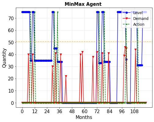
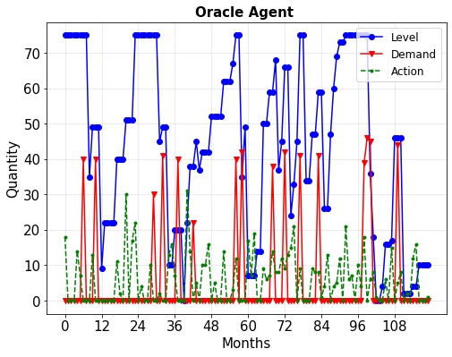
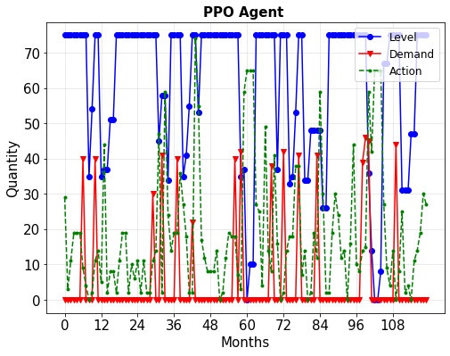
Figure 2: Inventory level (blue) of an item (ID=$21$) over $T=120$ months with different agents: MinMax (left), Oracle (center), PPO (right). The demand is plotted in red and the order actions are plotted in green. The safety stock MinMax agent is displayed in orange.

Agents battle. In order to evaluate the performance of the developed approach, different baselines are implemented along with the reinforcement learning methods.

• MinMax agents: a standard min-max strategy $(s,S)$ from operation research. For these agents, each item has a safety stock $\kappa=\Phi^{-1}(\alpha)\sqrt{(\mu_{\tau}\sigma_{\delta}^{2})+(\mu_{\delta}\sigma_{\tau})^{2}}$, where $\Phi$ is the c.d.f. of $\mathcal{N}(0,1)$, $\alpha\in\{0.90,0.95,0.99\}$ represents the target service level and $\mu,\sigma^{2}$ are the mean and variance of the demands and lead-times. The value of the service level is set to the classical value $\alpha=0.90$ and the means and variances are computed using the MLE estimators. As soon as the inventory level goes below the safety stock, the controller orders the maximum capacity of the corresponding item. Note that such approach is easy to implement but may fail to anticipate spikes in the demand signal.

• Oracle agents: such agents implement the following heuristic: given the knowledge of the mean $\mu_{\delta}$ and variance $\sigma_{\delta}^{2}$ of the demand signal, it is natural to order, at each timestep, according to a random law with mean $\mu_{\delta}$ and variance $\sigma_{\delta}^{2}$. More precisely, the oracle agents have access to the estimated mean $\hat{\mu}_{\delta}$ and standard deviation $\hat{\sigma}_{\delta}$ of their associated products and order at each time according to a normal law $\mathcal{N}(\hat{\mu}_{\delta},\hat{\sigma}_{\delta}^{2})$ which is clamped to fit the bounds of the action space.

• MARL agents: the reinforcement learning agents are trained using Proximal Policy Optimization (PPO) algorithms [46] which are stable and effective policy gradient methods. When working with capacity constraints per item, both discrete (Eq. (1)) and continuous (Eq.(2)) policies are considered, denoted by PPO-D and PPO-C respectively. When the items compete for storage space, IPPO [54] which is an independent version of PPO for multi-agent frameworks is implemented. The different parameter configurations are given in Appendix A.

Results. In the idea that similar items among a cluster share some intrinsic features, the question of generalization for a single agent is raised. For that matter, first consider a scenario with a cluster of $5$ items with their own capacity constraints and a single RL agent trained on an average item, i.e., a ”virtual” item whose features are given by taking the mean of the features of all the items in that cluster is trained. Then the learned behavior on the $5$ items of the cluster is tested and the different cumulative costs are reported. Table 1 below presents the average cumulative costs in $ obtained over $100$ replications of the different methods for the $5$ items over an horizon of $T=240$ months.

ID	MinMax	Oracle	PPO-D	PPO-C
0	48,554,986	10,183,088	4,863,202	4,616,016
1	52,993,931	16,917,389	6,865,991	6,385,378
2	70,467,282	21,426,806	8,727,215	8,087,258
3	72,220,832	12,722,887	9,854,047	5,280,345
4	79,235,272	16,976,630	8,801,628	4,808,191

Table 1: Average Cumulative cost in $ over 100 replications for different items over $T=240$ months.

ID	0	1	2	3	4
MinMax	39	41	42	51	49
Oracle	10	11	13	8	10
PPO-D	0	0	0	0	0
PPO-C	0	0	0	0	0

Table 2: Average Item Shortage over 100 replications for different items over $T=240$ months.

Regarding the average cumulative costs, the clear winners are the RL-based methods. Indeed, the PPO methods are statistically better than the two other baselines with a cost reduction factor ranging from $8$ (for item ID=1) to $16$ (for item ID=4) compared to the standard $(s,S)$-strategy. Interestingly, among the PPO methods, the one with continuous actions presents the best performance. Another important result concerns the number of items shortages as shown by Table 2 above. Once again, the RL-based methods outperform the two standard baselines. Furthermore, the PPO agents learned an optimal strategy in terms of stock-outs since the number of item shortages is always equal to zero. Such careful behavior is confirmed by Figure 2 where the evolution of the inventory levels is plotted, over an horizon of $T=120$ months, for a particular item according to the different strategies. Note that compared to the MinMax and Oracle agents, the inventory levels of the PPO agent are always above the demand signal which ensure the avoidance of stock-outs. Interestingly, the RL agents have the nice following interpretation: whenever there is either a demand spike or a demand plateau for a long time, there is an incentive to order. Additional numerical results concerning all $50$ different items are available in Appendices C and D for the average cumulative costs and the average item shortages respectively.

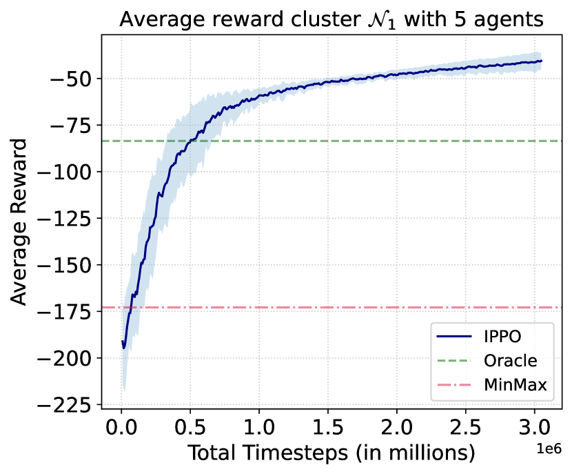
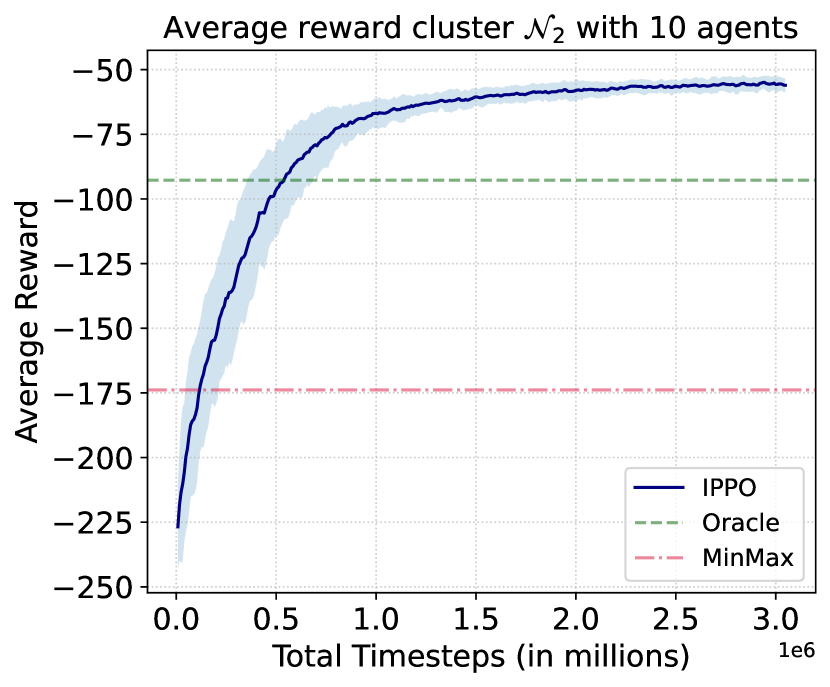
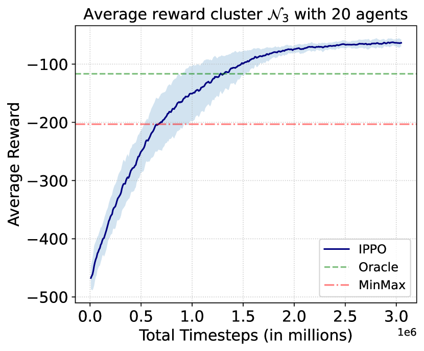
Figure 3: Learning curves for the different clusters $\mathcal{N}_{1},\mathcal{N}_{2}$ and $\mathcal{N}_{3}$ where the mean and standard deviation of IPPO are plotted in blue and the horizontal lines represent the average reward for the two baselines Oracle (green) and MinMax (red) computed over $100$ replications.

Another scenario involving storage capacity constraint is considered with three different clusters $\mathcal{N}_{1},\mathcal{N}_{2}$ and $\mathcal{N}_{3}$ composed of $5,10$ and $20$ items respectively. The last cluster represents a more complex task as it involves many agents. As before, the different methods based on the average cumulative cost over a cluster and the average item shortages over a cluster are compared, both over an horizon of $T=240$ months. For each cluster, one may take a look at the different training curves of the MARL agents. Such training is repeated on $10$ replications and the results are displayed in Figure 3 which gathers the evolution of the normalized average reward along the training episodes. The means and standard deviations of the average reward of the MARL agents are plotted in blue. For ease of comparison, two horizontal lines corresponding to the normalized average reward of the MinMax and Oracle agents are added. Thus, it allows to check the performance gain obtained with the RL-based methods compared to standard baselines. Observe that for clusters $\mathcal{N}_{1}$ and $\mathcal{N}_{2}$, the MARL agents quickly outperform the baselines in approximately $500,000$ timesteps but need more than 1M timesteps on cluster $\mathcal{N}_{3}$ to surpass the Oracle agents. Concerning the test performance of the learned behaviors, the different Tables below show the average cumulative cost and average stock-outs over the different items, obtained over $100$ replications and an horizon of $T=240$ months.

Cluster	$\mathcal{N}_{1}$	$\mathcal{N}_{2}$	$\mathcal{N}_{3}$
MinMax	49,219,195	55,148,027	63,319,299
Oracle	29,596,024	31,047,144	38,002,027
IPPO-C	12,048,666	7,905,165	14,239,567

Table 3: Average Cumulative cost in $ over different clusters, computed over 100 replications for an horizon of $T=240$ months.

Cluster	$\mathcal{N}_{1}$	$\mathcal{N}_{2}$	$\mathcal{N}_{3}$
MinMax	18	18	23
Oracle	13	9	11
IPPO-C	3	0	2

Table 4: Average Item shortages computed over 100 replications for an horizon of $T=240$ months.

Once again, the MARL-based agents present the best performance, both in terms of cost savings (see Table 4) and avoidance of shortages (see Table 4). Observe that for cluster $\mathcal{N}_{1}$, the MARL agents allows an overall cost reduction of $75\%$ compared to the standard $(s,S)$ strategy, $85\%$ for cluster $\mathcal{N}_{2}$ and about $78\%$ for cluster $\mathcal{N}_{3}$. For each cluster, the details about the average costs and shortages of all items are available in Appendix E.

6 Conclusion & Discussion

Maintaining the right balance between the supply and demand of products by optimizing replenishment decisions is one of the most important challenges for inventory management systems. In this paper, a rigorous methodological and practical reinforcement learning framework to address the inventory management problem for a single-echelon multi-products supply chain on a production line with stochastic demands and lead-times has been developed. The method has been illustrated with extensive numerical experiments on real data for both single and multi-agents algorithms.

This problem is very close to real-world use cases. Not only does it handle stochastic demands and lead-times but is designed for deployment as an actual business solution on production lines. Future work will focus on the statistical properties of the developed framework by further exploring links with mean-field approximation theory and the effects of exogenous variables in reinforcement learning.

Appendix

Appendix A collects the technical details related to the implementation of Proximal Policy Optimization algorithms, namely the different loss functions and the associated hyper-parameters used for the training phase. Appendix B gathers the different item parameters of the real data. Appendices C and D present additional results concerning the cumulative costs and item shortages for single agents. Similarly, Appendix E is dedicated to the detailed numerical results of MARL based methods.

Appendix A Proximal Policy Optimization algorithms

A.1 PPO methodology and model

PPO is a model-free on-policy RL algorithm that works well for both discrete and continuous action space environments. PPO utilizes an actor-critic framework, where there are two networks, an actor (policy network) and critic network (value function). Such algorithms are part of the family of policy gradient algorithms which use a parameterized action-selection policy $\pi_{\theta}$ with $\theta\in\Theta\subset\mathbb{R}^{d}$ and update the policy parameter $\theta$ on each step in the direction of an estimate of the gradient of the performance with respect to the policy parameter:

$$\theta\leftarrow\theta+\eta\hat{g},$$

where $\eta$ is the learning rate, $\hat{g}=\mathbb{E}_{t}[\nabla_{\theta}\log\pi_{\theta}(a_{t}|s_{t})\hat{A}_{t}]$ is a gradient estimate, $\hat{A}_{t}$ is an estimator of the advantage function at timestep $t$ and the expectation $\mathbb{E}_{t}$ indicates the empirical average over a finite batch of samples, in an algorithm that alternates between sampling and optimization.

The implementation of the Proximal Policy Optimization algorithms follows the one of the open-source library RLlib [33]. Whereas standard policy gradient methods perform one gradient update per data sample, PPO enables multiple epochs of minibatch updates. According to [46], compared to TRPO methods, PPO algorithms are much simpler to implement, more general, and have better sample complexity (empirically). PPO’s clipped objective supports multiple SGD passes over the same batch of experiences and RLlib’s PPO can scale out using multiple workers for experience collection, and also with multiple GPUs for SGD.

Denote by $r_{t}(\theta)=\pi_{\theta}(a_{t}|s_{t})/\pi_{\theta_{\text{old}}}(a_{t}|s_{t})$ the probability ratio between old and new policies so that TRPO methods aim at optimizing the following surrogate objective: $\mathcal{L}_{\text{TRPO}}(\theta)=\mathbb{E}_{t}[r_{t}(\theta)\hat{A}_{t}]$. In comparison, PPO methods rely on the following clipped objective function:

$$\mathcal{L}_{\text{actor}}(\theta)=\mathbb{E}_{t}\left[\min\left\{r_{t}(\theta)\hat{A}_{t},\text{clip}(r_{t}(\theta),1-\varepsilon,1+\varepsilon)\hat{A}_{t}\right\}\right].$$

The motivation for this objective is as follows. The second term inside the min modifies the surrogate objective by clipping the probability ratio, which removes the incentive for moving $r_{t}$ outside of the interval $[1-\varepsilon,1+\varepsilon]$. By taking the minimum of the clipped and unclipped objective, the final objective is a lower bound (i.e., a pessimistic bound) on the unclipped objective. With this scheme, PPO methods only ignore the change in probability ratio when it would make the objective improve, and include it when it makes the objective worse. This very idea of clipping can also be applied to the critic whose aim is to approximate the value function using some neural network, leading to the following critic loss

$$\mathcal{L}_{\text{critic}}(\theta)=\mathbb{E}_{t}\left[\max\left\{(V_{\theta}(s_{t})-\hat{V}_{t})^{2},(V_{\theta_{\text{old}}}(s_{t})-\hat{V}_{t}+\text{clip}(V_{\theta}(s_{t})-V_{\theta_{\text{old}}}(s_{t}),-\varepsilon,+\varepsilon))^{2}\right\}\right]$$

Furthermore, in addition to clipped surrogate objective, consider some KL divergence and entropy terms. For the KL term, this follows from the fact that a certain surrogate objective (which computes the max KL over states instead of the mean) forms a lower bound (i.e., a pessimistic bound) on the performance of the current policy. Finally, the total objective can be augmented by adding an entropy bonus $\mathcal{H}$ to ensure sufficient exploration, as suggested in past work [35]. Overall, the goal is to maximize the following objective function

$$\mathcal{L}(\theta)=\mathcal{L}_{\text{actor}}(\theta)-c_{1}\mathcal{L}_{\text{critic}}(\theta)-c_{2}\mathbb{E}_{t}[D_{KL}(\pi_{\theta_{\text{old}}}(\cdot|s_{t}),\pi_{\theta}(\cdot|s_{t}))]+c_{3}\mathbb{E}_{t}[\mathcal{H}(\pi_{\theta})(s_{t})],$$

where $\mathcal{L}_{\text{actor}}$ is the policy loss, $\mathcal{L}_{\text{critic}}$ is the critic loss, $D_{KL}$ is the Kullback-Liebler divergence and $\mathcal{H}$ is the entropy bonus. The constants $c_{1},c_{2}$ and $c_{3}$ are the value-function loss coefficient, the KL coefficient and the entropy coefficient.

A.2 Implementation Details

When working with storage constraints per item, it is enough to only train a few agents. The $50$ items of the different warehouses are split in $2$ groups according to the median of lead-time in order to train only $2$ average RL agent. Such agents are then tested on all the items in the corresponding group. In order to compare the effect of working with discrete or continuous actions spaces, two RL agents are trained using Discrete actions (PPO-D1 and PPO-D2), and 2 RL agents using Continuous actions (PPO-C1 and PPO-C2). When working with items competing for storage space, MARL algorithms are used, suchg as IPPO and other variations with shared critic. Tables 5 and 6 gather all the details about the different hyper parameters used for the traning of (MA)RL agents. In all the experiments, the following parameters are fixed:

Parameter	Value
HORIZON	200
GAMMA	0.99
LEARNING RATE	1e-4
VF SHARE LAYERS	False
ROLLOUT FRAGMENTLENGTH	200
BATCHMODE	complete
TRAIN BATCH SIZE	8000
SGD MINIBACTH SIZE	250
NUM SGD ITER	20
NORMALIZE ACTIONS	True
FCNET ACTIVATION	relu
USE CRITIC	True
GAE LAMBDA	1
KL COEFF	2e-1
KL TARGET	1e-2
ENTROPY COEFF	0.01
CLIP PARAM	0.3

Table 5: Hyper parameters Details for Training

The following parameters are specific to the different RL agents:

Parameter	PPO-D1	PPO-D2	PPO-C1	PPO-D2
FCNET HIDDEN	[512, 512]	[512, 512]	[512, 512]	[512, 512]
GRAD CLIP	40	40	40	40
LEARNING RATE	1e-4	1e-4	1e-4	2e-4
VF SHARE LAYERS	False	False	False	False
USE GAE	True	True	True	True
VF CLIP PARAM	1e3	1e4	1e3	5e2
VF LOSS COEFF	1	1e-2	1e-2	1e-2

Table 6: Hyper parameters Details for Training

Parameter	IPPO-$\mathcal{N}_{1}$	IPPO-$\mathcal{N}_{2}$	IPPO-$\mathcal{N}_{3}$
FCNET HIDDEN	[512, 256]	[512,256]	[512,256]
GRAD CLIP	40	20	20
LEARNING RATE	5e-5	2e-5	2e-5
VF SHARE LAYERS	True	True	True
USE GAE	False	False	False
VF CLIP PARAM	5e2	5e2	5e2
VF LOSS COEFF	1e-3	1e-4	1e-4

Table 7: Hyper parameters Details for Training

Appendix B Item Hyperparameters

The data is used to find the model parameters of the stochastic distributions using some MLE estimators. For a fixed item $i\in\mathcal{N}$ with historical data of demands $(\delta_{t}^{(i)})_{t=1,\ldots,N_{i}}$ and lead-times $(\tau_{t}^{(i)})_{t=1,\ldots,T_{i}}$, the MLE estimators $\hat{b}_{i},\hat{\mu}_{i}$ and $\hat{p}_{i}$ are given by the empirical averages

$$\hat{b}_{i}=\frac{1}{N_{i}}\sum_{t=1}^{N_{i}}\mathds{1}_{\{\delta_{t}^{(i)}>0\}}\qquad\hat{\mu}_{i}=\frac{\sum_{t=1}^{N_{i}}\delta_{t}^{(i)}\mathds{1}_{\{\delta_{t}^{(i)}>0\}}}{\sum_{t=1}^{N_{i}}\mathds{1}_{\{\delta_{t}^{(i)}>0\}}}\qquad\hat{p}_{i}=\frac{T_{i}}{\sum_{t=1}^{T_{i}}\tau_{t}^{(i)}}$$

The different Tables below summarize the parameter values for each item.

ID	$\hat{b}$	$\hat{\mu}$	$\hat{p}$	$C_{o}$	$C_{h}$	$C_{s}$
0	0.33	6.23	0.12	1,010	57	11,097
1	0.12	17.33	0.17	1,092	125	11,800
2	0.21	11.0	0.17	1,363	159	14,887
3	0.24	9.04	0.11	1,125	131	12,881
4	0.17	12.0	0.11	1,007	119	14,758
5	0.31	6.87	0.11	1,174	65	15,954
6	0.17	12.5	0.12	1,280	104	18,109
7	0.12	17.25	0.12	1,220	71	14,450
8	0.18	11.82	0.19	2,250	269	23,984
9	0.29	8.46	0.13	1,356	129	13,998

Table 8: Products Parameters and Costs for Items 0-9

ID	$\hat{b}$	$\hat{\mu}$	$\hat{p}$	$C_{o}$	$C_{h}$	$C_{s}$
10	0.29	8.08	0.15	1,597	170	21,512
11	0.11	22.0	0.14	1,069	100	14,184
12	0.4	8.25	0.2	1,020	112	15,244
13	0.17	16.25	0.15	1,342	149	14,059
14	0.15	20.59	0.12	1,080	112	11,352
15	0.08	24.0	0.41	3,380	298	37,941
16	0.24	9.83	0.1	1,857	194	23,874
17	0.12	26.67	0.14	1,042	107	11,000
18	0.12	20.0	0.1	1,360	174	17,718
19	0.4	7.07	0.12	1,690	215	20,403

Table 9: Products Parameters and Costs for Items 10-19

ID	$\hat{b}$	$\hat{\mu}$	$\hat{p}$	$C_{o}$	$C_{h}$	$C_{s}$
20	0.08	40.0	0.15	1,110	95	12,873
21	0.38	9.5	0.12	1,270	181	13,578
22	0.08	32.67	0.1	1,276	184	16,441
23	0.17	23.58	0.2	1,170	60	15,026
24	0.14	20.4	0.11	2,084	270	25,725
25	0.08	40.0	0.12	1,371	177	14,804
26	0.11	32.5	0.09	1,092	152	12,305
27	0.08	32.0	0.11	2,104	135	24,015
28	0.11	36.5	0.15	1,252	139	14,186
29	0.39	7.81	0.1	1,792	93	25,279

Table 10: Products Parameters and Costs for Items 20-29

ID	$\hat{b}$	$\hat{\mu}$	$\hat{p}$	$C_{o}$	$C_{h}$	$C_{s}$
30	0.28	15.25	0.1	1,085	77	14,038
31	0.08	40.0	0.08	1,445	164	14,742
32	0.19	18.3	0.11	2,284	304	23,957
33	0.26	19.73	0.16	1,142	138	13,926
34	0.17	26.0	0.15	1,342	196	16,559
35	0.33	10.39	0.07	1,851	267	19,626
36	0.14	26.0	0.15	1,765	225	25,052
37	0.1	35.67	0.11	2,070	130	20,910
38	0.12	30.17	0.09	1,380	204	20,550
39	0.33	6.58	0.06	4,470	456	51,326

Table 11: Products Parameters and Costs for Items 30-39

ID	$\hat{b}$	$\hat{\mu}$	$\hat{p}$	$C_{o}$	$C_{h}$	$C_{s}$
40	0.29	18.14	0.17	1,689	158	22,534
41	0.08	50.0	0.1	1,329	141	17,654
42	0.22	20.77	0.13	2,312	257	29,177
43	0.44	14.33	0.1	1,308	100	15,170
44	0.08	70.0	0.1	1,308	179	13,718
45	0.17	34.0	0.18	3,590	328	38,035
46	0.08	108.0	0.12	1,011	87	10,134
47	0.19	111.0	0.12	1,049	100	15,621
48	0.18	97.88	0.11	1,851	171	20,451
49	0.08	217.0	0.11	1,851	114	25,362

Table 12: Products Parameters and Costs for Items 40-49

Appendix C Average Cumulative Costs

C.1 Numerical Results

The different Tables below present the full results of cumulative costs for the numerical experiments with storage space constraints per item. The $50$ items are split in $2$ groups according to the median of lead-time in order to train only $2$ average RL agent. Such agents are then tested on all the items in the corresponding group.

ID	MinMax	Oracle	PPO-D	PPO-C
0	48,554,986	10,183,088	4,863,202	4,616,016
1	52,993,931	16,917,389	6,865,991	6,385,378
2	70,467,282	21,426,806	8,727,215	8,087,258
3	72,220,832	12,722,887	9,854,047	5,280,345
4	79,235,272	16,976,630	8,801,628	4,808,191
5	79,945,152	17,793,765	9,068,217	4,270,027
6	94,856,066	23,070,095	6,725,252	6,330,215
7	94,888,885	23,194,601	9,540,166	4,599,449
8	96,678,620	30,082,381	15,010,899	13,646,991
9	98,917,563	15,738,319	7,593,699	7,229,608

Table 13: Average Cumulative Costs in $ obtained over $100$ replications, horizon of $T=240$ months for Items 0-9.

ID	MinMax	Oracle	PPO-D	PPO-C
10	110,582,575	24,999,881	9,564,232	9,038,083
11	112,399,072	42,910,634	7,574,747	6,628,323
12	115,603,447	46,823,147	6,853,628	6,103,570
13	124,832,231	39,888,919	8,243,508	7,665,907
14	152,157,505	47,941,527	6,445,518	6,418,000
15	156,482,922	64,905,614	26,221,197	18,708,044
16	162,805,503	32,745,666	15,653,937	8,462,765
17	165,864,536	74,037,166	10,165,442	9,631,728
18	167,274,515	46,875,740	12,546,177	7,122,270
19	174,895,434	56,821,488	10,050,155	9,706,447

Table 14: Average Cumulative Costs in $ obtained over $100$ replications, horizon of $T=240$ months for Items 10-19.

ID	MinMax	Oracle	PPO-D	PPO-C
20	182,267,502	130,132,350	33,743,915	36,077,127
21	188,855,483	66,602,602	8,227,594	7,704,383
22	209,851,096	101,916,137	18,964,499	19,156,603
23	240,876,429	119,152,696	10,058,032	9,181,690
24	253,729,788	94,653,074	18,857,686	14,191,791
25	259,717,238	154,572,208	39,887,428	41,316,087
26	275,654,944	136,723,841	21,806,460	28,917,117
27	294,354,320	13,3290,131	25,792,146	22,497,325
28	297,756,076	195,971,759	34,602,990	39,975,903
29	317,748,541	78,399,969	13,360,829	6,625,366

Table 15: Average Cumulative Costs in $ obtained over $100$ replications, horizon of $T=240$ months for Items 20-29.

ID	MinMax	Oracle	PPO-D	PPO-C
30	340,850,617	118,356,448	8,428,058	5,674,420
31	346,677,835	165,513,863	38,211,495	50,257,711
32	372,022,376	140,849,611	20,580,162	13,426,053
33	379,189,787	176,014,600	17,857,314	12,033,561
34	379,417,845	187,467,258	20,350,345	18,721,088
35	429,201,653	125,815,263	15,920,620	10,148,258
36	450,249,676	197,138,780	20,805,554	21,535,008
37	467,942,296	221,381,388	40,233,046	51,880,344
38	517,401,650	217,431,556	25,188,489	35,934,573
39	529,054,715	113,253,016	35,899,378	19,663,470

Table 16: Average Cumulative Costs in $ obtained over $100$ replications, horizon of $T=240$ months for Items 30-39.

ID	MinMax	Oracle	PPO-D	PPO-C
40	548,632,612	274,992,151	19,614,638	14,265,377
41	614,478,713	351,832,711	91,357,970	158,742,424
42	802,247,508	318,672,823	28,692,777	22,605,438
43	826,810,789	277,103,747	13,143,955	18,262,774
44	897,278,509	593,855,529	278,916,815	434,302,595
45	1205,603,289	856,462,764	193,219,445	184,847,412
46	1463,640,790	1196,188,961	1013,385,300	1137,694,029
47	7013,730,126	5018,246,734	4692,465,941	5153,720,918
48	7033,366,188	4830,858,675	4348,154,722	4928,213,014
49	10354,442,106	9275,492,362	9137,883,131	9309,276,387

Table 17: Average Cumulative Costs in $ obtained over $100$ replications, horizon of $T=240$ months for Items 40-49.

C.2 Barplots results

Similarly to Section C.1, the different barplots below present the full results of cumulative costs for the numerical experiments with storage space constraints per item. The $50$ items are split in $2$ groups according to the median of lead-time in order to train only $2$ average RL agent. Such agents are then tested on all the items in the corresponding group.

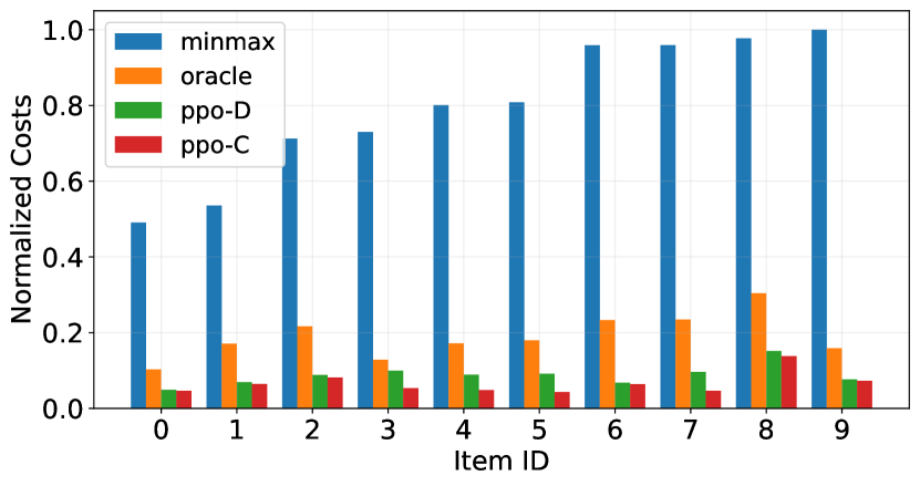
Figure 4: Average Cumulative Costs in $ obtained over $100$ replications, horizon of $T=240$ months for Items 0-9.

Figure 5: Average Cumulative Costs in $ obtained over $100$ replications, horizon of $T=240$ months for Items 10-19.

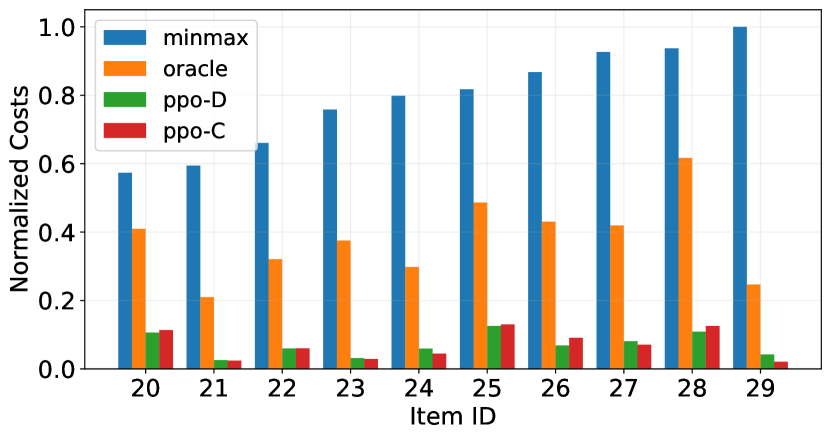
Figure 6: Average Cumulative Costs in $ obtained over $100$ replications, horizon of $T=240$ months for Items 20-29.

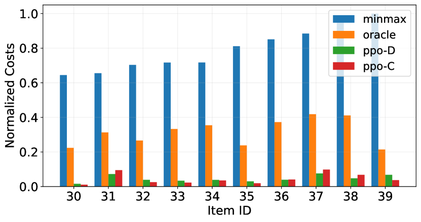
Figure 7: Average Cumulative Costs in $ obtained over $100$ replications, horizon of $T=240$ months for Items 30-39.

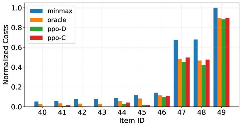
Figure 8: Average Cumulative Costs in $ obtained over $100$ replications, horizon of $T=240$ months for Items 40-49.

Appendix D Average Item Shortages

D.1 Numerical results

The different Tables below present the full results of item shortages for the numerical experiments with storage space constraints per item. The $50$ items are split in $2$ groups according to the median of lead-time in order to train only $2$ average RL agent. Such agents are then tested on all the items in the corresponding group.

ID	MinMax	Oracle	PPO-D	PPO-C
0	39	10	0	0
1	41	11	0	0
2	42	13	0	0
3	51	8	0	0
4	49	10	0	0
5	43	10	0	0
6	47	11	0	0
7	57	12	0	0
8	38	10	0	0
9	59	9	0	0

Table 18: Average Item shortages obtained over $100$ replications, horizon of $T=240$ months for Items 0-9.

ID	MinMax	Oracle	PPO-D	PPO-C
10	44	11	0	0
11	69	23	0	0
12	66	26	0	0
13	76	25	0	0
14	119	37	0	0
15	37	14	0	0
16	65	13	0	0
17	132	58	2	2
18	84	22	0	0
19	71	26	0	0

Table 19: Average Item shortages obtained over $100$ replications, horizon of $T=240$ months for Items 10-19.

ID	MinMax	Oracle	PPO-D	PPO-C
20	125	84	16	17
21	119	41	0	0
22	108	52	3	5
23	132	69	1	1
24	95	29	0	0
25	155	88	16	16
26	200	89	7	14
27	109	46	2	4
28	182	114	15	18
29	109	26	0	0

Table 20: Average Item shortages obtained over $100$ replications, horizon of $T=240$ months for Items 20-29.

ID	MinMax	Oracle	PPO-D	PPO-C
30	219	69	0	0
31	209	94	14	22
32	140	48	0	0
33	234	110	4	2
34	196	95	6	5
35	197	49	0	0
36	155	66	3	3
37	193	89	9	16
38	220	86	5	11
39	90	18	0	0

Table 21: Average Item shortages obtained over $100$ replications, horizon of $T=240$ months for Items 30-39.

ID	MinMax	Oracle	PPO-D	PPO-C
40	209	102	2	1
41	305	172	40	75
42	240	95	3	3
43	472	141	1	5
44	575	360	167	264
45	276	186	35	33
46	1230	986	837	945
47	3814	2695	2520	2770
48	2959	1989	1778	2030
49	3453	3066	3025	3081

Table 22: Average Item shortages obtained over $100$ replications, horizon of $T=240$ months for Items 40-49.

D.2 Barplots results

Similarly to Section D.1, the different barplots below present the full results of item shortages for the numerical experiments with storage space constraints per item. The $50$ items are split in $2$ groups according to the median of lead-time in order to train only $2$ average RL agent. Such agents are then tested on all the items in the corresponding group.

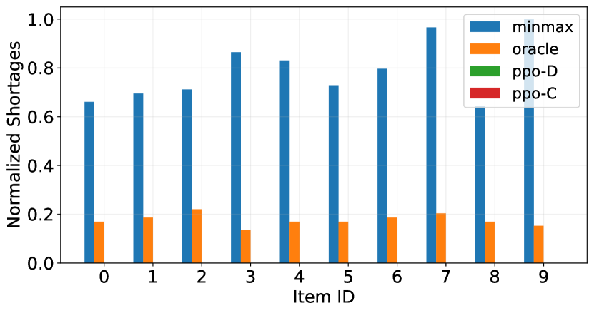
Figure 9: Average Item shortages obtained over $100$ replications, horizon of $T=240$ months for Items 0-9.

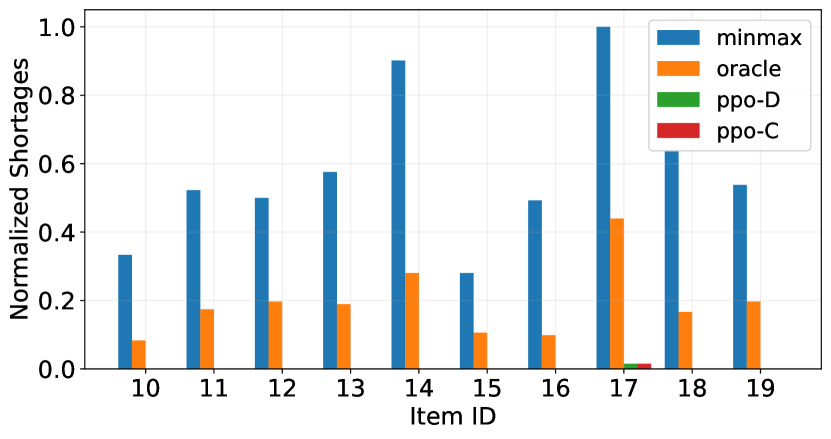
Figure 10: Average Item shortages obtained over $100$ replications, horizon of $T=240$ months for Items 10-19.

Figure 11: Average Item shortages obtained over $100$ replications, horizon of $T=240$ months for Items 20-29.

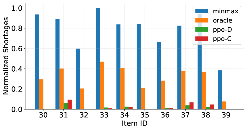
Figure 12: Average Item shortages obtained over $100$ replications, horizon of $T=240$ months for Items 30-39.

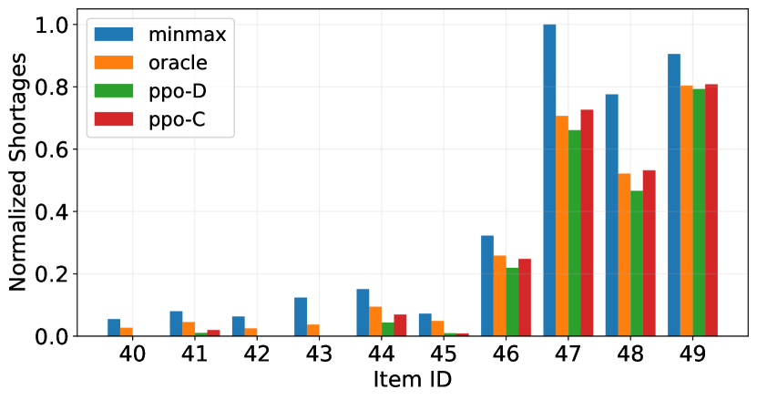
Figure 13: Average Item shortages obtained over $100$ replications, horizon of $T=240$ months for Items 40-49.

Appendix E Average Cumulative Costs and Item Shortages for Multi-Agent cases

E.1 Cluster $\mathcal{N}_{1}$

ID	MinMax	Oracle	IPPO-C
$\mathcal{N}_{1}$-0	56,413,703	47,751,643	21,747,138
$\mathcal{N}_{1}$-1	41,218,939	22,017,147	5,860,091
$\mathcal{N}_{1}$-2	28,734,942	10,052,437	9,674,691
$\mathcal{N}_{1}$-3	69,445,374	49,567,318	11,468,600
$\mathcal{N}_{1}$-4	50,283,017	18,591,579	11,492,810
Average	49,219,195	29,596,024	12,048,666

Table 23: Average Cumulative Costs in $ obtained over $100$ replications, horizon of $T=240$ months for cluster $\mathcal{N}_{1}$

ID	MinMax	Oracle	IPPO-C
$\mathcal{N}_{1}$-0	27	25	0
$\mathcal{N}_{1}$-1	18	10	1
$\mathcal{N}_{1}$-2	11	4	6
$\mathcal{N}_{1}$-3	22	21	5
$\mathcal{N}_{1}$-4	14	5	3
Average	18	9	3

Table 24: Average Item Shortages obtained over $100$ replications, horizon of $T=240$ months for cluster $\mathcal{N}_{1}$

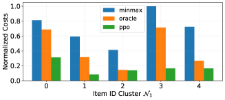
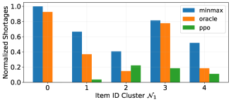
Figure 14: Average Cumulative Costs in $ and Item Shortages obtained over $100$ replications, horizon of $T=240$ months for cluster $\mathcal{N}_{1}$

E.2 Cluster $\mathcal{N}_{2}$

ID	MinMax	Oracle	IPPO-C
$\mathcal{N}_{2}$-0	61,746,686	37,154,240	9,576,664
$\mathcal{N}_{2}$-1	43,195,470	19,817,180	4,755,388
$\mathcal{N}_{2}$-2	31,719,337	8,849,048	7,232,925
$\mathcal{N}_{2}$-3	49,873,610	38,995,232	7,999,544
$\mathcal{N}_{2}$-4	46,383,922	17,470,651	8,097,309
$\mathcal{N}_{2}$-5	90,361,502	54,257,529	6,974,378
$\mathcal{N}_{2}$-6	20,349,092	8,573,083	4,180,512
$\mathcal{N}_{2}$-7	27,434,488	9,091,921	9,855,567
$\mathcal{N}_{2}$-8	33,681,010	11,145,783	3,862,856
$\mathcal{N}_{2}$-9	146,735,155	105,116,776	16,516,513
Average	55,148,027	31,047,144	7,905,165

Table 25: Average Cumulative Costs in $ obtained over $100$ replications, horizon of $T=240$ months for cluster $\mathcal{N}_{2}$

ID	MinMax	Oracle	IPPO-C
$\mathcal{N}_{2}$-0	33	18	1
$\mathcal{N}_{2}$-1	18	8	0
$\mathcal{N}_{2}$-2	14	2	0
$\mathcal{N}_{2}$-3	16	14	0
$\mathcal{N}_{2}$-4	13	4	0
$\mathcal{N}_{2}$-5	27	16	0
$\mathcal{N}_{2}$-6	11	8	0
$\mathcal{N}_{2}$-7	11	2	0
$\mathcal{N}_{2}$-8	14	5	0
$\mathcal{N}_{2}$-9	20	13	0
Average	18	9	0

Table 26: Average Item Shortages obtained over $100$ replications, horizon of $T=240$ months for cluster $\mathcal{N}_{2}$

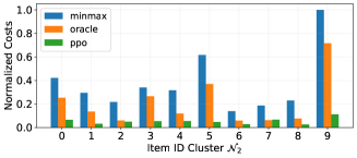
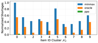
Figure 15: Average Cumulative Costs in $ and Item Shortages obtained over $100$ replications, horizon of $T=240$ months for cluster $\mathcal{N}_{2}$

E.3 Cluster $\mathcal{N}_{3}$

ID	MinMax	Oracle	IPPO-C
$\mathcal{N}_{3}$-0	114,748,999	110,936,731	25,133,542
$\mathcal{N}_{3}$-1	76,876,589	25,248,863	13,012,784
$\mathcal{N}_{3}$-2	175,969,893	156,867,720	22,712,799
$\mathcal{N}_{3}$-3	61,746,686	38,243,787	11,097,544
$\mathcal{N}_{3}$-4	43,195,470	14,974,424	6,590,003
$\mathcal{N}_{3}$-5	31,719,337	9,423,716	12,452,378
$\mathcal{N}_{3}$-6	49,873,610	35,928,930	13,922,411
$\mathcal{N}_{3}$-7	46,383,922	20,756,443	7,299,909
$\mathcal{N}_{3}$-8	34,654,173	9,843,404	11,531,224
$\mathcal{N}_{3}$-9	90,361,502	55,657,119	13,186,238
$\mathcal{N}_{3}$-10	20,349,092	8,662,162	5,354,639
$\mathcal{N}_{3}$-11	41,008,234	12,947,589	10,195,819
$\mathcal{N}_{3}$-12	33,335,933	12,451,461	10,197,750
$\mathcal{N}_{3}$-13	27,434,488	8,713,145	8,518,849
$\mathcal{N}_{3}$-14	33,681,010	10,451,041	8,045,677
$\mathcal{N}_{3}$-15	106,676,800	56,572,852	11,317,268
$\mathcal{N}_{3}$-16	146,735,155	126,683,713	55,932,376
$\mathcal{N}_{3}$-17	46,569,841	24,907,569	14,623,596
$\mathcal{N}_{3}$-18	41,120,038	9,885,961	13,659,858
$\mathcal{N}_{3}$-19	43,945,213	10,883,913	10,006,678
Average	63,319,299	38,002,027	14,239,567

Table 27: Average Cumulative Costs in $ obtained over $100$ replications, horizon of $T=240$ months for cluster $\mathcal{N}_{3}$

ID	MinMax	Oracle	IPPO-C
$\mathcal{N}_{3}$-0	39	33	7
$\mathcal{N}_{3}$-1	19	4	0
$\mathcal{N}_{3}$-2	97	63	0
$\mathcal{N}_{3}$-3	33	19	1
$\mathcal{N}_{3}$-4	18	5	0
$\mathcal{N}_{3}$-5	14	4	6
$\mathcal{N}_{3}$-6	16	14	4
$\mathcal{N}_{3}$-7	13	5	0
$\mathcal{N}_{3}$-8	15	2	2
$\mathcal{N}_{3}$-9	27	17	4
$\mathcal{N}_{3}$-10	11	6	1
$\mathcal{N}_{3}$-11	9	0	0
$\mathcal{N}_{3}$-12	13	3	3
$\mathcal{N}_{3}$-13	11	3	0
$\mathcal{N}_{3}$-14	14	4	2
$\mathcal{N}_{3}$-15	55	22	0
$\mathcal{N}_{3}$-16	20	18	2
$\mathcal{N}_{3}$-17	19	7	7
$\mathcal{N}_{3}$-18	14	2	0
$\mathcal{N}_{3}$-19	16	2	3
Average	23	11	2

Table 28: Average Item Shortages obtained over $100$ replications, horizon of $T=240$ months for cluster $\mathcal{N}_{3}$

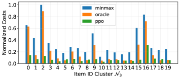
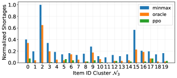
Figure 16: Average Cumulative Costs in $ and Item Shortages obtained over $100$ replications, horizon of $T=240$ months for cluster $\mathcal{N}_{3}$

References

- Adler and Blue, [2002] Adler, J. L. and Blue, V. J. (2002). A cooperative multi-agent transportation management and route guidance system. Transportation Research Part C: Emerging Technologies, 10(5-6):433–454.
- Barat et al., [2019] Barat, S., Khadilkar, H., Meisheri, H., Kulkarni, V., Baniwal, V., Kumar, P., and Gajrani, M. (2019). Actor based simulation for closed loop control of supply chain using reinforcement learning. In Proceedings of the 18th international conference on autonomous agents and multiagent systems, pages 1802–1804.
- Başar and Olsder, [1998] Başar, T. and Olsder, G. J. (1998). Dynamic noncooperative game theory. SIAM.
- Baxter and Bartlett, [2001] Baxter, J. and Bartlett, P. L. (2001). Infinite-horizon policy-gradient estimation. Journal of Artificial Intelligence Research, 15:319–350.
- Bellman, [1966] Bellman, R. (1966). Dynamic programming. Science, 153(3731):34–37.
- Bellman and Dreyfus, [1959] Bellman, R. and Dreyfus, S. (1959). Functional approximations and dynamic programming. Mathematical Tables and Other Aids to Computation, pages 247–251.
- Bellman and Kalaba, [1957] Bellman, R. and Kalaba, R. (1957). Dynamic programming and statistical communication theory. Proceedings of the National Academy of Sciences of the United States of America, 43(8):749.
- Bertsekas, [2011] Bertsekas, D. P. (2011). Approximate policy iteration: A survey and some new methods. Journal of Control Theory and Applications, 9(3):310–335.
- Bertsekas and Tsitsiklis, [1996] Bertsekas, D. P. and Tsitsiklis, J. N. (1996). Neuro-dynamic programming, volume 5. Athena Scientific Belmont, MA.
- Buşoniu et al., [2012] Buşoniu, L., Lazaric, A., Ghavamzadeh, M., Munos, R., Babuška, R., and De Schutter, B. (2012). Least-squares methods for policy iteration. Reinforcement learning, pages 75–109.
- Chaharsooghi et al., [2008] Chaharsooghi, S. K., Heydari, J., and Zegordi, S. H. (2008). A reinforcement learning model for supply chain ordering management: An application to the beer game. Decision Support Systems, 45(4):949–959.
- Chaudhary et al., [2018] Chaudhary, V., Kulshrestha, R., and Routroy, S. (2018). State-of-the-art literature review on inventory models for perishable products. Journal of Advances in Management Research.
- Corke et al., [2005] Corke, P., Peterson, R., and Rus, D. (2005). Networked robots: Flying robot navigation using a sensor net. In Robotics research. The eleventh international symposium, pages 234–243. Springer.
- Dall’Anese et al., [2013] Dall’Anese, E., Zhu, H., and Giannakis, G. B. (2013). Distributed optimal power flow for smart microgrids. IEEE Transactions on Smart Grid, 4(3):1464–1475.
- Doan et al., [2019] Doan, T., Maguluri, S., and Romberg, J. (2019). Finite-time analysis of distributed td (0) with linear function approximation on multi-agent reinforcement learning. In International Conference on Machine Learning, pages 1626–1635. PMLR.
- Dogan and Güner, [2015] Dogan, I. and Güner, A. R. (2015). A reinforcement learning approach to competitive ordering and pricing problem. Expert Systems, 32(1):39–48.
- Fang et al., [2013] Fang, J., Zhao, L., Fransoo, J. C., and Van Woensel, T. (2013). Sourcing strategies in supply risk management: An approximate dynamic programming approach. Computers & Operations Research, 40(5):1371–1382.
- Filar and Vrieze, [2012] Filar, J. and Vrieze, K. (2012). Competitive Markov decision processes. Springer Science & Business Media.
- Fisher, [1922] Fisher, R. A. (1922). On the mathematical foundations of theoretical statistics. Philosophical Transactions of the Royal Society of London. Series A, Containing Papers of a Mathematical or Physical Character, 222(594-604):309–368.
- Fukuda, [1964] Fukuda, Y. (1964). Optimal policies for the inventory problem with negotiable leadtime. Management Science, 10(4):690–708.
- Giannoccaro and Pontrandolfo, [2002] Giannoccaro, I. and Pontrandolfo, P. (2002). Inventory management in supply chains: a reinforcement learning approach. International Journal of Production Economics, 78(2):153–161.
- Gijsbrechts et al., [2021] Gijsbrechts, J., Boute, R. N., Van Mieghem, J. A., and Zhang, D. (2021). Can deep reinforcement learning improve inventory management? performance on dual sourcing, lost sales and multi-echelon problems. Manufacturing & Service Operations Management.
- Halman et al., [2009] Halman, N., Klabjan, D., Mostagir, M., Orlin, J., and Simchi-Levi, D. (2009). A fully polynomial-time approximation scheme for single-item stochastic inventory control with discrete demand. Mathematics of Operations Research, 34(3):674–685.
- Howard, [1960] Howard, R. A. (1960). Dynamic programming and markov processes.
- Jiang and Sheng, [2009] Jiang, C. and Sheng, Z. (2009). Case-based reinforcement learning for dynamic inventory control in a multi-agent supply-chain system. Expert Systems with Applications, 36(3):6520–6526.
- Khouja and Goyal, [2008] Khouja, M. and Goyal, S. (2008). A review of the joint replenishment problem literature: 1989–2005. European Journal of Operational Research, 186(1):1–16.
- Kim et al., [2005] Kim, C., Jun, J., Baek, J., Smith, R., and Kim, Y.-D. (2005). Adaptive inventory control models for supply chain management. The International Journal of Advanced Manufacturing Technology, 26(9):1184–1192.
- Kim et al., [2008] Kim, C. O., Kwon, I.-H., and Baek, J.-G. (2008). Asynchronous action-reward learning for nonstationary serial supply chain inventory control. Applied Intelligence, 28(1):1–16.
- Kober et al., [2013] Kober, J., Bagnell, J. A., and Peters, J. (2013). Reinforcement learning in robotics: A survey. The International Journal of Robotics Research, 32(11):1238–1274.
- Kwak et al., [2009] Kwak, C., Choi, J. S., Kim, C. O., and Kwon, I.-H. (2009). Situation reactive approach to vendor managed inventory problem. Expert Systems with Applications, 36(5):9039–9045.
- Kwon et al., [2008] Kwon, I.-H., Kim, C. O., Jun, J., and Lee, J. H. (2008). Case-based myopic reinforcement learning for satisfying target service level in supply chain. Expert Systems with applications, 35(1-2):389–397.
- Levi et al., [2014] Levi, D. S., Chen, X., and Bramel, J. (2014). The logic of logistics: theory, algorithms, and applications for logistics management. Springer.
- Liang et al., [2018] Liang, E., Liaw, R., Nishihara, R., Moritz, P., Fox, R., Goldberg, K., Gonzalez, J., Jordan, M., and Stoica, I. (2018). Rllib: Abstractions for distributed reinforcement learning. In International Conference on Machine Learning, pages 3053–3062. PMLR.
- Littman, [1994] Littman, M. L. (1994). Markov games as a framework for multi-agent reinforcement learning. In Machine learning proceedings 1994, pages 157–163. Elsevier.
- Mnih et al., [2015] Mnih, V., Kavukcuoglu, K., Silver, D., Rusu, A. A., Veness, J., Bellemare, M. G., Graves, A., Riedmiller, M., Fidjeland, A. K., Ostrovski, G., et al. (2015). Human-level control through deep reinforcement learning. nature, 518(7540):529–533.
- Nguyen et al., [2020] Nguyen, T. T., Nguyen, N. D., and Nahavandi, S. (2020). Deep reinforcement learning for multiagent systems: A review of challenges, solutions, and applications. IEEE transactions on cybernetics, 50(9):3826–3839.
- Okuda et al., [2014] Okuda, R., Kajiwara, Y., and Terashima, K. (2014). A survey of technical trend of adas and autonomous driving. In Technical Papers of 2014 International Symposium on VLSI Design, Automation and Test, pages 1–4. IEEE.
- Owen, [2001] Owen, A. B. (2001). Empirical likelihood. Chapman and Hall/CRC.
- Pineau et al., [2003] Pineau, J., Gordon, G., Thrun, S., et al. (2003). Point-based value iteration: An anytime algorithm for pomdps. In IJCAI, volume 3, pages 1025–1032. Citeseer.
- Porteus, [2002] Porteus, E. L. (2002). Foundations of stochastic inventory theory. Stanford University Press.
- Puterman, [1994] Puterman, M. L. (1994). Markov decision processes: discrete stochastic dynamic programming. John Wiley & Sons.
- Qu et al., [2015] Qu, H., Wang, L., and Liu, R. (2015). A contrastive study of the stochastic location-inventory problem with joint replenishment and independent replenishment. Expert Systems with Applications, 42(4):2061–2072.
- Rabbat and Nowak, [2004] Rabbat, M. and Nowak, R. (2004). Distributed optimization in sensor networks. In Proceedings of the 3rd international symposium on Information processing in sensor networks, pages 20–27.
- Salameh et al., [2014] Salameh, M. K., Yassine, A. A., Maddah, B., and Ghaddar, L. (2014). Joint replenishment model with substitution. Applied Mathematical Modelling, 38(14):3662–3671.
- Sallab et al., [2017] Sallab, A. E., Abdou, M., Perot, E., and Yogamani, S. (2017). Deep reinforcement learning framework for autonomous driving. Electronic Imaging, 2017(19):70–76.
- Schulman et al., [2017] Schulman, J., Wolski, F., Dhariwal, P., Radford, A., and Klimov, O. (2017). Proximal policy optimization algorithms. arXiv preprint arXiv:1707.06347.
- Shapley, [1953] Shapley, L. S. (1953). Stochastic games. Proceedings of the national academy of sciences, 39(10):1095–1100.
- Silver et al., [2018] Silver, D., Hubert, T., Schrittwieser, J., Antonoglou, I., Lai, M., Guez, A., Lanctot, M., Sifre, L., Kumaran, D., Graepel, T., et al. (2018). A general reinforcement learning algorithm that masters chess, shogi, and go through self-play. Science, 362(6419):1140–1144.
- Silver and Peterson, [1985] Silver, E. A. and Peterson, R. (1985). Decision systems for inventory management and production planning, volume 18. Wiley.
- Sondik, [1971] Sondik, E. J. (1971). The optimal control of partially observable markov processes. Technical report, Stanford Univ Calif Stanford Electronics Labs.
- Sultana et al., [2020] Sultana, N. N., Meisheri, H., Baniwal, V., Nath, S., Ravindran, B., and Khadilkar, H. (2020). Reinforcement learning for multi-product multi-node inventory management in supply chains. arXiv preprint arXiv:2006.04037.
- Sun and Zhao, [2012] Sun, R. and Zhao, G. (2012). Analyses about efficiency of reinforcement learning to supply chain ordering management. In IEEE 10th International Conference on Industrial Informatics, pages 124–127. IEEE.
- Sutton and Barto, [2018] Sutton, R. S. and Barto, A. G. (2018). Reinforcement learning: An introduction. MIT press.
- Tan, [1993] Tan, M. (1993). Multi-agent reinforcement learning: Independent vs. cooperative agents. In Proceedings of the tenth international conference on machine learning, pages 330–337.
- Toomey, [2000] Toomey, J. W. (2000). Inventory management: principles, concepts and techniques, volume 12. Springer Science & Business Media.
- Vinyals et al., [2019] Vinyals, O., Babuschkin, I., Czarnecki, W. M., Mathieu, M., Dudzik, A., Chung, J., Choi, D. H., Powell, R., Ewalds, T., Georgiev, P., et al. (2019). Grandmaster level in starcraft ii using multi-agent reinforcement learning. Nature, 575(7782):350–354.
- Wang et al., [2012] Wang, L., He, J., and Zeng, Y.-R. (2012). A differential evolution algorithm for joint replenishment problem using direct grouping and its application. Expert Systems, 29(5):429–441.
- Wang et al., [2015] Wang, L., Shi, Y., and Liu, S. (2015). An improved fruit fly optimization algorithm and its application to joint replenishment problems. Expert systems with Applications, 42(9):4310–4323.
- White, [1982] White, H. (1982). Maximum likelihood estimation of misspecified models. Econometrica: Journal of the econometric society, pages 1–25.
- Williams, [1992] Williams, R. J. (1992). Simple statistical gradient-following algorithms for connectionist reinforcement learning. Machine learning, 8(3):229–256.
- Zhang et al., [2021] Zhang, K., Yang, Z., and Başar, T. (2021). Multi-agent reinforcement learning: A selective overview of theories and algorithms. Handbook of Reinforcement Learning and Control, pages 321–384.
- Zhang et al., [2018] Zhang, K., Yang, Z., Liu, H., Zhang, T., and Basar, T. (2018). Fully decentralized multi-agent reinforcement learning with networked agents. In International Conference on Machine Learning, pages 5872–5881. PMLR.
- Zheng and Federgruen, [1991] Zheng, Y.-S. and Federgruen, A. (1991). Finding optimal (s, s) policies is about as simple as evaluating a single policy. Operations research, 39(4):654–665.
- Zipkin, [2000] Zipkin, P. H. (2000). Foundations of inventory management.