1. Introduction
Bulk-surface models have been used to describe a wide range of phenomena, from emulsions, foams stabilized by surface-active agents, to biological cell dynamics governed by proteins. Key to these models is the idea that the dynamics are not solely restricted to a bulk material, but that an active surface coating the bulk material, that is, a surface with its own dynamics, also dictates the overall material behaviour. Typically, these systems involve the adsorption of species onto the surface, giving rise to the particular dynamics found on the surface. These interactions may result in motion of the surface, which in turn may provoke bulk material deformation and the other way around. This bulk-surface reciprocal interplay is the focus of this work.
From a historical standpoint, a sharp interface of two-phase flow relates the surface traction at the interface with surface tension and curvature via a jump condition. Boussinesq [1 ] stipulated that a surface viscosity has to be incorporated in the interfacial constitutive law. As acknowledged by Bothe and Prüss [2 ] , Levich [3 ] also claimed that interfacial stresses may be induced by surface tension gradients due to the presence of surface-active particles, known as surfactants. The combination of such phenomena along with the mechanics of these material surfaces have been studied extensively. Adam [4 ] , Adamson [5 ] , and Scriven [6 ] were the pioneers in the physics and thermochemistry of material surfaces, as acknowledged by Gurtin & Murdoch [7 ] ; who also recast and systematically derived the underlying rational mechanics of bulk-surfaces materials.
Motivation for these bulk-surface continuum theories can for instance be found in biological systems. Cells may mathematically be described as a bulk material (cytoplasm) enclosed by a surface (cell membrane). Their mechanobiology involves various complex processes, as Ladoux & Mège [8 , Figure 1a] illustrate, which in turn determine the shape of these cells. In particular, during adhesion cells may take saucer-shaped forms. To fully understand the underlying mechanical behavior of these cells and such adhesive processes, the tractions developed on the edges need to be accounted for. Considering arbitrary geometries, including those with a boundary that may lose its smoothness, requires certain modifications and further generalization of continuum theories, as shown by Espath [9 ] for the Navier-Stokes equations. Furthermore, Brangwynne [10 ] and Shin & Brangwynne [11 ] suggest that membrane-less organelles are formed by regulated phase-segregation processes within the cytoplasm. In these works, the authors capitalize on the physics of polymer phase separation. Current frameworks that may capture the dynamics of these biological cells to some extent include the work by Madzvamuse et al. [12 ] , who present a reaction-diffusion for bulk-surface systems suitable to model cell polarization but do not include phase segregation and motion. In a similar fashion, Duda et al. [13 ] investigate bulk-surface systems for cell adsorption/desorption and chemical reactions for classical diffusion.
The objective of this work is to devise a continuum theory for bulk-surface materials undergoing deformation and phase segregation. In particular, we consider an immiscible binary bulk fluid enclosed by a thin immiscible binary fluid film that both deform in an incompressible manner. We treat this thin film as a material surface with finite thickness. Moreover, we assume that the material surface may lose smoothness, which gives rise to additional geometric contributions in the mathematical formulation. We depart by considering the motion of the bulk-surface material. Both bulk fluid and enclosing film of fluid undergo isochoric motions, that is, both flows are incompressible. Isochoric motion within the bulk implies no change in volume. However, isochoric motion within the thin film does not imply no change in surface area since the thickness of the surface may change. Based on these hypotheses, we derive the mass balance equations for the bulk and surface. This bulk-surface mass balance formalism is discussed in Section §2 [14 ] and present the coupled bulk-surface principle of virtual powers in Section §3 4 5 6 7 8 9
1.1. Differential tools
Consider a smooth surface 𝒮 𝒮 \mathcal{S} 𝒏 𝒏 \boldsymbol{n} 𝒙 ∈ 𝒮 𝒙 𝒮 \boldsymbol{x}\in\mathcal{S} 𝒮 𝒮 \mathcal{S} κ 𝜅 \kappa 𝜿 𝜿 \boldsymbol{\kappa} 𝐊 𝐊 \boldsymbol{\mathrm{{K}}} κ 𝜅 \kappa 𝜿 𝜿 \boldsymbol{\kappa} 𝐊 𝐊 \boldsymbol{\mathrm{{K}}} 𝒮 𝒮 \mathcal{S}
Bulk gradients may be written in the form
(1) grad κ = ∂ n κ 𝒏 + ∂ p κ 𝒆 p , and grad 𝜿 = ∂ n 𝜿 ⊗ 𝒏 + ∂ p 𝜿 ⊗ 𝒆 p , with p = 1 , 2 , formulae-sequence grad 𝜅 subscript 𝑛 𝜅 𝒏 subscript 𝑝 𝜅 superscript 𝒆 𝑝 and
formulae-sequence grad 𝜿 subscript 𝑛 tensor-product 𝜿 𝒏 subscript 𝑝 tensor-product 𝜿 superscript 𝒆 𝑝 with
𝑝 1 2
\mathrm{grad}\mskip 2.0mu\kappa=\partial_{n}\kappa\mskip 3.0mu\boldsymbol{n}+\partial_{p}\kappa\mskip 3.0mu\boldsymbol{e}^{p},\qquad\text{and}\qquad\mathrm{grad}\mskip 2.0mu\boldsymbol{\kappa}=\partial_{n}\boldsymbol{\kappa}\otimes\boldsymbol{n}+\partial_{p}\boldsymbol{\kappa}\otimes\boldsymbol{e}^{p},\qquad\text{with}\qquad p=1,2,
where the contravariant bases 𝒆 p superscript 𝒆 𝑝 \boldsymbol{e}^{p} 𝒮 𝒮 \mathcal{S} 𝒆 p = ∂ p 𝒙 subscript 𝒆 𝑝 subscript 𝑝 𝒙 \boldsymbol{e}_{p}=\partial_{p}\boldsymbol{x} 𝒙 ∈ 𝒮 𝒙 𝒮 \boldsymbol{x}\in\mathcal{S} 𝒆 p ⋅ 𝒆 q = δ p q ⋅ subscript 𝒆 𝑝 superscript 𝒆 𝑞 superscript subscript 𝛿 𝑝 𝑞 \boldsymbol{e}_{p}\cdot\boldsymbol{e}^{q}=\delta_{p}^{q} δ p q superscript subscript 𝛿 𝑝 𝑞 \delta_{p}^{q} 𝐏 𝒏 ≔ 𝐏 𝒏 ( 𝒏 ) ≔ subscript 𝐏 𝒏 subscript 𝐏 𝒏 𝒏 \boldsymbol{\mathrm{{P}}}_{\scriptscriptstyle{\mskip-6.0mu{\boldsymbol{n}}}}\coloneqq\boldsymbol{\mathrm{{P}}}_{\scriptscriptstyle{\mskip-6.0mu{\boldsymbol{n}}}}(\boldsymbol{n}) 𝒏 𝒏 \boldsymbol{n} 𝒙 ∈ 𝒮 𝒙 𝒮 \boldsymbol{x}\in\mathcal{S}
(2) 𝐏 𝒏 ≔ 𝟏 − 𝒏 ⊗ 𝒏 = 𝐏 𝒏 ⊤ , ≔ subscript 𝐏 𝒏 1 tensor-product 𝒏 𝒏 superscript subscript 𝐏 𝒏 top \boldsymbol{\mathrm{{P}}}_{\scriptscriptstyle{\mskip-6.0mu{\boldsymbol{n}}}}\coloneqq\boldsymbol{1}-\boldsymbol{n}\otimes\boldsymbol{n}=\boldsymbol{\mathrm{{P}}}_{\scriptscriptstyle{\mskip-6.0mu{\boldsymbol{n}}}}^{\scriptscriptstyle\mskip-1.0mu\top\mskip-2.0mu},
where ( ⋅ ) ⊤ superscript ⋅ top (\cdot)^{\scriptscriptstyle\mskip-1.0mu\top\mskip-2.0mu} 1 2
(3) grad 𝒮 κ ≔ ∂ p κ 𝒆 p = 𝐏 𝒏 grad κ , and grad 𝒮 𝜿 ≔ ∂ p 𝜿 ⊗ 𝒆 p = ( grad 𝜿 ) 𝐏 𝒏 , with p = 1 , 2 , formulae-sequence ≔ subscript grad 𝒮 𝜅 subscript 𝑝 𝜅 superscript 𝒆 𝑝 subscript 𝐏 𝒏 grad 𝜅 ≔ and subscript grad 𝒮 𝜿
subscript 𝑝 tensor-product 𝜿 superscript 𝒆 𝑝 grad 𝜿 subscript 𝐏 𝒏 with 𝑝
1 2 \mathrm{grad}\mskip 2.0mu_{\mskip-2.0mu\scriptscriptstyle\mathcal{S}}\kappa\coloneqq\partial_{p}\kappa\mskip 3.0mu\boldsymbol{e}^{p}=\boldsymbol{\mathrm{{P}}}_{\scriptscriptstyle{\mskip-6.0mu{\boldsymbol{n}}}}\mathrm{grad}\mskip 2.0mu\kappa,\qquad\text{and}\qquad\mathrm{grad}\mskip 2.0mu_{\mskip-2.0mu\scriptscriptstyle\mathcal{S}}\boldsymbol{\kappa}\coloneqq\partial_{p}\boldsymbol{\kappa}\otimes\boldsymbol{e}^{p}=(\mathrm{grad}\mskip 2.0mu\boldsymbol{\kappa})\boldsymbol{\mathrm{{P}}}_{\scriptscriptstyle{\mskip-6.0mu{\boldsymbol{n}}}},\qquad\text{with}\qquad p=1,2,
and surface divergences by
(4) div 𝒮 𝜿 ≔ ∂ p 𝜿 ⋅ 𝒆 p = grad 𝜿 : 𝐏 𝒏 , and div 𝒮 𝐊 ≔ ∂ p 𝐊 ⋅ 𝒆 p = grad 𝐊 : 𝐏 𝒏 with p = 1 , 2 . \mathrm{div}\mskip 2.0mu_{\mskip-6.0mu\scriptscriptstyle\mathcal{S}}\boldsymbol{\kappa}\coloneqq\partial_{p}\boldsymbol{\kappa}\cdot\boldsymbol{e}^{p}=\mathrm{grad}\mskip 2.0mu\boldsymbol{\kappa}\mskip 2.0mu\colon\mskip-2.0mu\boldsymbol{\mathrm{{P}}}_{\scriptscriptstyle{\mskip-6.0mu{\boldsymbol{n}}}},\qquad\text{and}\qquad\mathrm{div}\mskip 2.0mu_{\mskip-6.0mu\scriptscriptstyle\mathcal{S}}\boldsymbol{\mathrm{{K}}}\coloneqq\partial_{p}\boldsymbol{\mathrm{{K}}}\cdot\boldsymbol{e}^{p}=\mathrm{grad}\mskip 2.0mu\boldsymbol{\mathrm{{K}}}\mskip 2.0mu\colon\mskip-2.0mu\boldsymbol{\mathrm{{P}}}_{\scriptscriptstyle{\mskip-6.0mu{\boldsymbol{n}}}}\qquad\text{with}\qquad p=1,2.
Also, Laplace–Beltrami operators may be written as
(5) △ 𝒮 κ ≔ div 𝒮 grad 𝒮 κ = grad ( 𝐏 𝒏 grad κ ) : 𝐏 𝒏 , and △ 𝒮 𝜿 ≔ div 𝒮 grad 𝒮 𝜿 = grad ( ( grad 𝜿 ) 𝐏 𝒏 ) : 𝐏 𝒏 . : ≔ subscript △ 𝒮 𝜅 subscript div 𝒮 subscript grad 𝒮 𝜅 grad subscript 𝐏 𝒏 grad 𝜅 ≔ subscript 𝐏 𝒏 and subscript △ 𝒮 𝜿
subscript div 𝒮 subscript grad 𝒮 𝜿 grad grad 𝜿 subscript 𝐏 𝒏 : subscript 𝐏 𝒏 \triangle_{\mskip-2.0mu\scriptscriptstyle\mathcal{S}}\kappa\coloneqq\mathrm{div}\mskip 2.0mu_{\mskip-6.0mu\scriptscriptstyle\mathcal{S}}\mathrm{grad}\mskip 2.0mu_{\mskip-2.0mu\scriptscriptstyle\mathcal{S}}\kappa=\mathrm{grad}\mskip 2.0mu(\boldsymbol{\mathrm{{P}}}_{\scriptscriptstyle{\mskip-6.0mu{\boldsymbol{n}}}}\mathrm{grad}\mskip 2.0mu\kappa)\mskip 2.0mu\colon\mskip-2.0mu\boldsymbol{\mathrm{{P}}}_{\scriptscriptstyle{\mskip-6.0mu{\boldsymbol{n}}}},\qquad\text{and}\qquad\triangle_{\mskip-2.0mu\scriptscriptstyle\mathcal{S}}\boldsymbol{\kappa}\coloneqq\mathrm{div}\mskip 2.0mu_{\mskip-6.0mu\scriptscriptstyle\mathcal{S}}\mathrm{grad}\mskip 2.0mu_{\mskip-2.0mu\scriptscriptstyle\mathcal{S}}\boldsymbol{\kappa}=\mathrm{grad}\mskip 2.0mu((\mathrm{grad}\mskip 2.0mu\boldsymbol{\kappa})\boldsymbol{\mathrm{{P}}}_{\scriptscriptstyle{\mskip-6.0mu{\boldsymbol{n}}}})\mskip 2.0mu\colon\mskip-2.0mu\boldsymbol{\mathrm{{P}}}_{\scriptscriptstyle{\mskip-6.0mu{\boldsymbol{n}}}}.
Next, on a smooth closed oriented surface 𝒮 𝒮 \mathcal{S} 𝜿 𝜿 \boldsymbol{\kappa} 𝐊 𝐊 \boldsymbol{\mathrm{{K}}}
(6) ∫ 𝒮 div 𝒮 ( 𝐏 𝒏 𝜿 ) d a = 0 , and ∫ 𝒮 div 𝒮 ( 𝐊𝐏 𝒏 ) d a = 𝟎 , formulae-sequence subscript 𝒮 subscript div 𝒮 subscript 𝐏 𝒏 𝜿 differential-d 𝑎 0 and
subscript 𝒮 subscript div 𝒮 subscript 𝐊𝐏 𝒏 differential-d 𝑎 0 \int\limits_{\mathcal{S}}\mathrm{div}\mskip 2.0mu_{\mskip-6.0mu\scriptscriptstyle\mathcal{S}}(\boldsymbol{\mathrm{{P}}}_{\scriptscriptstyle{\mskip-6.0mu{\boldsymbol{n}}}}\boldsymbol{\kappa})\,\mathrm{d}a=0,\qquad\text{and}\qquad\int\limits_{\mathcal{S}}\mathrm{div}\mskip 2.0mu_{\mskip-6.0mu\scriptscriptstyle\mathcal{S}}(\boldsymbol{\mathrm{{K}}}\boldsymbol{\mathrm{{P}}}_{\scriptscriptstyle{\mskip-6.0mu{\boldsymbol{n}}}})\,\mathrm{d}a=\boldsymbol{0},
whereas, for any smooth vector and tensor fields 𝜿 𝜿 \boldsymbol{\kappa} 𝐊 𝐊 \boldsymbol{\mathrm{{K}}} 𝒮 𝒮 \mathcal{S}
(7) ∫ 𝒮 div 𝒮 ( 𝐏 𝒏 𝜿 ) d a = ∫ ∂ 𝒮 𝜿 ⋅ 𝝂 d σ , and ∫ 𝒮 div 𝒮 ( 𝐊𝐏 𝒏 ) d a = ∫ ∂ 𝒮 𝐊 𝝂 d σ , formulae-sequence subscript 𝒮 subscript div 𝒮 subscript 𝐏 𝒏 𝜿 differential-d 𝑎 subscript 𝒮 ⋅ 𝜿 𝝂 differential-d 𝜎 and
subscript 𝒮 subscript div 𝒮 subscript 𝐊𝐏 𝒏 differential-d 𝑎 subscript 𝒮 𝐊 𝝂 differential-d 𝜎 \int\limits_{\mathcal{S}}\mathrm{div}\mskip 2.0mu_{\mskip-6.0mu\scriptscriptstyle\mathcal{S}}(\boldsymbol{\mathrm{{P}}}_{\scriptscriptstyle{\mskip-6.0mu{\boldsymbol{n}}}}\boldsymbol{\kappa})\,\mathrm{d}a=\int\limits_{\partial\mathcal{S}}\boldsymbol{\kappa}\cdot\boldsymbol{\nu}\,\mathrm{d}\sigma,\qquad\text{and}\qquad\int\limits_{\mathcal{S}}\mathrm{div}\mskip 2.0mu_{\mskip-6.0mu\scriptscriptstyle\mathcal{S}}(\boldsymbol{\mathrm{{K}}}\boldsymbol{\mathrm{{P}}}_{\scriptscriptstyle{\mskip-6.0mu{\boldsymbol{n}}}})\,\mathrm{d}a=\int\limits_{\partial\mathcal{S}}\boldsymbol{\mathrm{{K}}}\boldsymbol{\nu}\,\mathrm{d}\sigma,
with 𝝂 𝝂 \boldsymbol{\nu} ∂ 𝒮 𝒮 \partial\mathcal{S}
Lastly, consider a nonsmooth oriented surface 𝒮 𝒮 \mathcal{S} 𝒞 𝒞 \mathcal{C} 𝒞 𝒞 \mathcal{C} 𝝂 + superscript 𝝂 \boldsymbol{\nu}^{+} 𝝂 − superscript 𝝂 \boldsymbol{\nu}^{-} 𝒞 𝒞 \mathcal{C} 𝒮 𝒮 \mathcal{S} 𝒮 ≔ 𝒮 + ∪ 𝒮 − ≔ 𝒮 superscript 𝒮 superscript 𝒮 \mathcal{S}\coloneqq\mathcal{S}^{+}\cup\mathcal{S}^{-} 𝒮 ≔ ⋃ α 𝒮 α ≔ 𝒮 subscript 𝛼 subscript 𝒮 𝛼 \mathcal{S}\coloneqq\bigcup_{\alpha}\mathcal{S}_{\alpha} 𝜿 𝜿 \boldsymbol{\kappa} 𝐊 𝐊 \boldsymbol{\mathrm{{K}}} 𝒞 𝒞 \mathcal{C} 𝜿 ± superscript 𝜿 plus-or-minus \boldsymbol{\kappa}^{\pm} 𝐊 ± superscript 𝐊 plus-or-minus \boldsymbol{\mathrm{{K}}}^{\pm} 𝜿 𝜿 \boldsymbol{\kappa} 𝐊 𝐊 \boldsymbol{\mathrm{{K}}} 𝒞 𝒞 \mathcal{C} 𝒮 ± superscript 𝒮 plus-or-minus \mathcal{S}^{\pm} 𝒞 𝒞 \mathcal{C} surplus , that is,
(8) ∫ 𝒮 div 𝒮 ( 𝐏 𝒏 𝜿 ) d a = ∫ 𝒞 { { 𝜿 ⋅ 𝝂 } } d σ , and ∫ 𝒮 div 𝒮 ( 𝐊𝐏 𝒏 ) d a = ∫ 𝒞 { { 𝐊 𝝂 } } d σ , formulae-sequence subscript 𝒮 subscript div 𝒮 subscript 𝐏 𝒏 𝜿 differential-d 𝑎 subscript 𝒞 ⋅ 𝜿 𝝂 differential-d 𝜎 and
subscript 𝒮 subscript div 𝒮 subscript 𝐊𝐏 𝒏 differential-d 𝑎 subscript 𝒞 𝐊 𝝂 differential-d 𝜎 \int\limits_{\mathcal{S}}\mathrm{div}\mskip 2.0mu_{\mskip-6.0mu\scriptscriptstyle\mathcal{S}}(\boldsymbol{\mathrm{{P}}}_{\scriptscriptstyle{\mskip-6.0mu{\boldsymbol{n}}}}\boldsymbol{\kappa})\,\mathrm{d}a=\int\limits_{\mathcal{C}}\{\!\!\{{\boldsymbol{\kappa}\cdot\boldsymbol{\nu}}\}\!\!\}\,\mathrm{d}\sigma,\qquad\text{and}\qquad\int\limits_{\mathcal{S}}\mathrm{div}\mskip 2.0mu_{\mskip-6.0mu\scriptscriptstyle\mathcal{S}}(\boldsymbol{\mathrm{{K}}}\boldsymbol{\mathrm{{P}}}_{\scriptscriptstyle{\mskip-6.0mu{\boldsymbol{n}}}})\,\mathrm{d}a=\int\limits_{\mathcal{C}}\{\!\!\{{\boldsymbol{\mathrm{{K}}}\boldsymbol{\nu}}\}\!\!\}\,\mathrm{d}\sigma,
where { { 𝜿 ⋅ 𝝂 } } ≔ 𝜿 + ⋅ 𝝂 + + 𝜿 − ⋅ 𝝂 − ≔ ⋅ 𝜿 𝝂 ⋅ superscript 𝜿 superscript 𝝂 ⋅ superscript 𝜿 superscript 𝝂 \{\!\!\{{\boldsymbol{\kappa}\cdot\boldsymbol{\nu}}\}\!\!\}\coloneqq\boldsymbol{\kappa}^{+}\cdot\boldsymbol{\nu}^{+}+\boldsymbol{\kappa}^{-}\cdot\boldsymbol{\nu}^{-} { { 𝐊 𝝂 } } ≔ 𝐊 + 𝝂 + + 𝐊 − 𝝂 − ≔ 𝐊 𝝂 superscript 𝐊 superscript 𝝂 superscript 𝐊 superscript 𝝂 \{\!\!\{{\boldsymbol{\mathrm{{K}}}\boldsymbol{\nu}}\}\!\!\}\coloneqq\boldsymbol{\mathrm{{K}}}^{+}\boldsymbol{\nu}^{+}+\boldsymbol{\mathrm{{K}}}^{-}\boldsymbol{\nu}^{-} 8
(9) ∫ 𝒮 div 𝒮 ( 𝐏 𝒏 𝜿 ) d a = ∫ ∂ 𝒮 𝜿 ⋅ 𝝂 d σ + ∫ 𝒞 { { 𝜿 ⋅ 𝝂 } } d σ , and ∫ 𝒮 div 𝒮 ( 𝐊𝐏 𝒏 ) d a = ∫ ∂ 𝒮 𝐊 𝝂 d σ + ∫ 𝒞 { { 𝐊 𝝂 } } d σ . formulae-sequence subscript 𝒮 subscript div 𝒮 subscript 𝐏 𝒏 𝜿 differential-d 𝑎 subscript 𝒮 ⋅ 𝜿 𝝂 differential-d 𝜎 subscript 𝒞 ⋅ 𝜿 𝝂 differential-d 𝜎 and
subscript 𝒮 subscript div 𝒮 subscript 𝐊𝐏 𝒏 differential-d 𝑎 subscript 𝒮 𝐊 𝝂 differential-d 𝜎 subscript 𝒞 𝐊 𝝂 differential-d 𝜎 \int\limits_{\mathcal{S}}\mathrm{div}\mskip 2.0mu_{\mskip-6.0mu\scriptscriptstyle\mathcal{S}}(\boldsymbol{\mathrm{{P}}}_{\scriptscriptstyle{\mskip-6.0mu{\boldsymbol{n}}}}\boldsymbol{\kappa})\,\mathrm{d}a=\int\limits_{\partial\mathcal{S}}\boldsymbol{\kappa}\cdot\boldsymbol{\nu}\,\mathrm{d}\sigma+\int\limits_{\mathcal{C}}\{\!\!\{{\boldsymbol{\kappa}\cdot\boldsymbol{\nu}}\}\!\!\}\,\mathrm{d}\sigma,\qquad\text{and}\qquad\int\limits_{\mathcal{S}}\mathrm{div}\mskip 2.0mu_{\mskip-6.0mu\scriptscriptstyle\mathcal{S}}(\boldsymbol{\mathrm{{K}}}\boldsymbol{\mathrm{{P}}}_{\scriptscriptstyle{\mskip-6.0mu{\boldsymbol{n}}}})\,\mathrm{d}a=\int\limits_{\partial\mathcal{S}}\boldsymbol{\mathrm{{K}}}\boldsymbol{\nu}\,\mathrm{d}\sigma+\int\limits_{\mathcal{C}}\{\!\!\{{\boldsymbol{\mathrm{{K}}}\boldsymbol{\nu}}\}\!\!\}\,\mathrm{d}\sigma.
2. Isochoric motion & mass balance
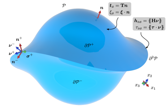
In the reference configuration, we consider a material body 𝒫 𝒫 \mathcal{P} ℰ ℰ \mathcal{E} 𝒫 𝒫 \mathcal{P} ∂ 𝒫 𝒫 \partial\mathcal{P} ∂ 2 𝒫 superscript 2 𝒫 \partial^{2}\mathcal{P} 1 ∂ 2 𝒫 superscript 2 𝒫 \partial^{2}\mathcal{P} ∂ 𝒫 ± superscript 𝒫 plus-or-minus \partial\mathcal{P}^{\pm} ∂ 𝒫 ± superscript 𝒫 plus-or-minus \partial\mathcal{P}^{\pm} ∂ 2 𝒫 superscript 2 𝒫 \partial^{2}\mathcal{P} { 𝒏 + , 𝒏 − } superscript 𝒏 superscript 𝒏 \{\boldsymbol{n}^{+},\boldsymbol{n}^{-}\} ∂ 2 𝒫 superscript 2 𝒫 \partial^{2}\mathcal{P} ∂ 𝒫 ± superscript 𝒫 plus-or-minus \partial\mathcal{P}^{\pm} ∂ 2 𝒫 superscript 2 𝒫 \partial^{2}\mathcal{P} { 𝝂 + , 𝝂 − } superscript 𝝂 superscript 𝝂 \{\boldsymbol{\nu}^{+},\boldsymbol{\nu}^{-}\} ∂ 2 𝒫 superscript 2 𝒫 \partial^{2}\mathcal{P} 𝝈 ≔ 𝝈 + ≔ 𝝈 superscript 𝝈 \boldsymbol{\sigma}\coloneqq\boldsymbol{\sigma}^{+} 𝝈 + ≔ 𝒏 + × 𝝂 + ≔ superscript 𝝈 superscript 𝒏 superscript 𝝂 \boldsymbol{\sigma}^{+}\coloneqq\boldsymbol{n}^{+}\times\boldsymbol{\nu}^{+} τ 𝜏 \tau 𝒫 τ subscript 𝒫 𝜏 \mathcal{P}_{\tau} ∂ 𝒫 τ subscript 𝒫 𝜏 \partial\mathcal{P}_{\tau} 𝒫 τ subscript 𝒫 𝜏 \mathcal{P}_{\tau} ∂ 2 𝒫 τ superscript 2 subscript 𝒫 𝜏 \partial^{2}\mathcal{P}_{\tau} ∂ 𝒫 τ subscript 𝒫 𝜏 \partial\mathcal{P}_{\tau} 𝒫 𝒫 \mathcal{P} ∂ 𝒫 𝒫 \partial\mathcal{P} ∂ 2 𝒫 superscript 2 𝒫 \partial^{2}\mathcal{P}
Figure 1. (Adapted from [14 ] , licensed under CC-BY 4.0). Part 𝒫 𝒫 \mathcal{P} ∂ 𝒫 ± superscript 𝒫 plus-or-minus \partial\mathcal{P}^{\pm} 𝒏 𝒏 \boldsymbol{n} 𝝂 ± superscript 𝝂 plus-or-minus \boldsymbol{\nu}^{\pm} ∂ 2 𝒫 superscript 2 𝒫 \partial^{2}\mathcal{P} 𝝈 ≔ 𝒏 × 𝝂 ≔ 𝝈 𝒏 𝝂 \boldsymbol{\sigma}\coloneqq\boldsymbol{n}\times\boldsymbol{\nu} ∂ 𝒫 𝒫 \partial\mathcal{P} ∂ 2 𝒫 superscript 2 𝒫 \partial^{2}\mathcal{P}
In this continuum theory, the bulk and surface material are endowed with two distinct kinematic descriptors, namely, the fluid velocities 𝝊 𝒫 subscript 𝝊 𝒫 \boldsymbol{\upsilon}_{\scriptscriptstyle\mathcal{P}} 𝝊 ∂ 𝒫 subscript 𝝊 𝒫 \boldsymbol{\upsilon}_{\scriptscriptstyle\partial\mathcal{P}} ϱ 𝒫 subscript italic-ϱ 𝒫 \varrho_{\scriptscriptstyle\mathcal{P}} ϱ ∂ 𝒫 subscript italic-ϱ 𝒫 \varrho_{\scriptscriptstyle\partial\mathcal{P}} ℓ τ subscript ℓ 𝜏 \ell_{\tau}
In what follows, we assume that
(A.1)
The ‘bulk-surface motion’ is isochoric. For the bulk material, this means that motion preserves its volumes. For the surface material, we assume that isochoric motion implies volume conservation on a microscopic scale.
(A.2)
The normal components of the velocities are continuous, that is,
(10) 𝝊 𝒫 ⋅ 𝒏 | ∂ 𝒫 = 𝝊 ∂ 𝒫 ⋅ 𝒏 . evaluated-at ⋅ subscript 𝝊 𝒫 𝒏 𝒫 ⋅ subscript 𝝊 𝒫 𝒏 \boldsymbol{\upsilon}_{\scriptscriptstyle\mathcal{P}}\cdot\boldsymbol{n}\big{|}_{\partial\mathcal{P}}=\boldsymbol{\upsilon}_{\scriptscriptstyle\partial\mathcal{P}}\cdot\boldsymbol{n}.
The kinematic constraint (10 10 ∂ 2 𝒫 superscript 2 𝒫 \partial^{2}\mathcal{P}
(11) 𝝊 𝒫 ⋅ 𝒏 + | ∂ 2 𝒫 = 𝝊 ∂ 𝒫 ⋅ 𝒏 + | ∂ 2 𝒫 , and 𝝊 𝒫 ⋅ 𝒏 − | ∂ 2 𝒫 = 𝝊 ∂ 𝒫 ⋅ 𝒏 − | ∂ 2 𝒫 . formulae-sequence evaluated-at ⋅ subscript 𝝊 𝒫 superscript 𝒏 superscript 2 𝒫 evaluated-at ⋅ subscript 𝝊 𝒫 superscript 𝒏 superscript 2 𝒫 and
evaluated-at ⋅ subscript 𝝊 𝒫 superscript 𝒏 superscript 2 𝒫 evaluated-at ⋅ subscript 𝝊 𝒫 superscript 𝒏 superscript 2 𝒫 \boldsymbol{\upsilon}_{\scriptscriptstyle\mathcal{P}}\cdot\boldsymbol{n}^{+}\big{|}_{\partial^{2}\mathcal{P}}=\boldsymbol{\upsilon}_{\scriptscriptstyle\partial\mathcal{P}}\cdot\boldsymbol{n}^{+}\big{|}_{\partial^{2}\mathcal{P}},\quad\text{and}\quad\boldsymbol{\upsilon}_{\scriptscriptstyle\mathcal{P}}\cdot\boldsymbol{n}^{-}\big{|}_{\partial^{2}\mathcal{P}}=\boldsymbol{\upsilon}_{\scriptscriptstyle\partial\mathcal{P}}\cdot\boldsymbol{n}^{-}\big{|}_{\partial^{2}\mathcal{P}}.
With these assumptions in mind, let
(12) 𝐅 𝒫 ≔ grad 𝒙 𝒚 𝒫 , and 𝐅 ∂ 𝒫 ≔ grad 𝒮 𝒙 𝒚 ∂ 𝒫 , formulae-sequence ≔ subscript 𝐅 𝒫 superscript grad 𝒙 subscript 𝒚 𝒫 and
≔ subscript 𝐅 𝒫 superscript subscript grad 𝒮 𝒙 subscript 𝒚 𝒫 \boldsymbol{\mathrm{{F}}}_{\!\scriptscriptstyle\mathcal{P}}\coloneqq\mathrm{grad}\mskip 2.0mu^{\!\boldsymbol{x}}\boldsymbol{y}_{\scriptscriptstyle\mathcal{P}},\quad\text{and}\quad\boldsymbol{\mathrm{{F}}}_{\!\scriptscriptstyle\partial\mathcal{P}}\coloneqq\mathrm{grad}\mskip 2.0mu_{\mskip-2.0mu\scriptscriptstyle\mathcal{S}}^{\!\boldsymbol{x}}\boldsymbol{y}_{\scriptscriptstyle\partial\mathcal{P}},
denote the bulk and surface deformation gradient with respect to the reference configuration, either 𝒙 𝒫 ∈ 𝒫 subscript 𝒙 𝒫 𝒫 \boldsymbol{x}_{\scriptscriptstyle\mathcal{P}}\in\mathcal{P} 𝒙 ∂ 𝒫 ∈ ∂ 𝒫 subscript 𝒙 𝒫 𝒫 \boldsymbol{x}_{\scriptscriptstyle\partial\mathcal{P}}\in\partial\mathcal{P} 𝒚 𝒫 subscript 𝒚 𝒫 \boldsymbol{y}_{\scriptscriptstyle\mathcal{P}} 𝒫 τ subscript 𝒫 𝜏 \mathcal{P}_{\tau} 𝒚 ∂ 𝒫 subscript 𝒚 𝒫 \boldsymbol{y}_{\scriptscriptstyle\partial\mathcal{P}} ∂ 𝒫 τ subscript 𝒫 𝜏 \partial\mathcal{P}_{\tau} 𝒫 τ = 𝒚 𝒫 ( 𝒫 ) subscript 𝒫 𝜏 subscript 𝒚 𝒫 𝒫 \mathcal{P}_{\tau}=\boldsymbol{y}_{\scriptscriptstyle\mathcal{P}}(\mathcal{P}) ∂ 𝒫 τ = 𝒚 ∂ 𝒫 ( ∂ 𝒫 ) subscript 𝒫 𝜏 subscript 𝒚 𝒫 𝒫 \partial\mathcal{P}_{\tau}=\boldsymbol{y}_{\scriptscriptstyle\partial\mathcal{P}}(\partial\mathcal{P}) 𝒚 𝒫 subscript 𝒚 𝒫 \boldsymbol{y}_{\scriptscriptstyle\mathcal{P}} 𝒚 ∂ 𝒫 subscript 𝒚 𝒫 \boldsymbol{y}_{\scriptscriptstyle\partial\mathcal{P}} s ˙ ≔ ∂ t s + 𝝊 𝒫 ⋅ grad s ≔ ˙ 𝑠 subscript 𝑡 𝑠 ⋅ subscript 𝝊 𝒫 grad 𝑠 \dot{s}\coloneqq\partial_{t}s+\boldsymbol{\upsilon}_{\scriptscriptstyle\mathcal{P}}\cdot\mathrm{grad}\mskip 2.0mus ∂ t subscript 𝑡 \partial_{t} [15 ] , and is given by
(13) s ̊ ≔ s □ + 𝝊 ∂ 𝒫 ⋅ grad 𝒮 s , ≔ ̊ 𝑠 □ 𝑠 ⋅ subscript 𝝊 𝒫 subscript grad 𝒮 𝑠 \mathring{s}\coloneqq\overset{\scriptscriptstyle\square}{s}+\boldsymbol{\upsilon}_{\scriptscriptstyle\partial\mathcal{P}}\cdot\mathrm{grad}\mskip 2.0mu_{\mskip-2.0mu\scriptscriptstyle\mathcal{S}}s,
where the normal time derivative is
(14) s □ ≔ d d ε ( s ( 𝒚 ∂ 𝒫 + ε ( 𝝊 ∂ 𝒫 ( 𝒚 ∂ 𝒫 , t ) ⋅ 𝒏 ( 𝒚 ∂ 𝒫 ) ) 𝒏 ( 𝒚 ∂ 𝒫 ) , t + ε ) ) | ε = 0 . ≔ □ 𝑠 evaluated-at d d 𝜀 𝑠 subscript 𝒚 𝒫 𝜀 ⋅ subscript 𝝊 𝒫 subscript 𝒚 𝒫 𝑡 𝒏 subscript 𝒚 𝒫 𝒏 subscript 𝒚 𝒫 𝑡 𝜀 𝜀 0 \overset{\scriptscriptstyle\square}{s}\coloneqq\dfrac{\text{d}}{\text{d}\varepsilon}\Big{(}s(\boldsymbol{y}_{\scriptscriptstyle\partial\mathcal{P}}+\varepsilon(\boldsymbol{\upsilon}_{\scriptscriptstyle\partial\mathcal{P}}(\boldsymbol{y}_{\scriptscriptstyle\partial\mathcal{P}},t)\cdot\boldsymbol{n}(\boldsymbol{y}_{\scriptscriptstyle\partial\mathcal{P}}))\boldsymbol{n}(\boldsymbol{y}_{\scriptscriptstyle\partial\mathcal{P}}),t+\varepsilon)\Big{)}\Big{|}_{\varepsilon=0}.
Since 𝐅 ∂ 𝒫 subscript 𝐅 𝒫 \boldsymbol{\mathrm{{F}}}_{\!\scriptscriptstyle\partial\mathcal{P}}
(15) 𝐅 ∂ 𝒫 − 1 ≔ 𝐏 n ( 𝒙 ∂ 𝒫 ) ( 𝐅 ∂ 𝒫 + 𝒏 ( 𝒚 ∂ 𝒫 ) ⊗ 𝒏 ( 𝒙 ∂ 𝒫 ) ) − 1 , ≔ superscript subscript 𝐅 𝒫 1 subscript 𝐏 𝑛 subscript 𝒙 𝒫 superscript subscript 𝐅 𝒫 tensor-product 𝒏 subscript 𝒚 𝒫 𝒏 subscript 𝒙 𝒫 1 \boldsymbol{\mathrm{{F}}}_{\!\scriptscriptstyle\partial\mathcal{P}}^{-1}\coloneqq\boldsymbol{\mathrm{{P}}}_{\scriptscriptstyle{\mskip-6.0mu{n}}}(\boldsymbol{x}_{\scriptscriptstyle\partial\mathcal{P}})(\boldsymbol{\mathrm{{F}}}_{\!\scriptscriptstyle\partial\mathcal{P}}+\boldsymbol{n}(\boldsymbol{y}_{\scriptscriptstyle\partial\mathcal{P}})\otimes\boldsymbol{n}(\boldsymbol{x}_{\scriptscriptstyle\partial\mathcal{P}}))^{-1},
where we explicitly show the dependency on either the reference configuration 𝒙 ∂ 𝒫 ∈ ∂ 𝒫 subscript 𝒙 𝒫 𝒫 \boldsymbol{x}_{\scriptscriptstyle\partial\mathcal{P}}\in\partial\mathcal{P} 𝒚 ∂ 𝒫 ∈ ∂ 𝒫 τ subscript 𝒚 𝒫 subscript 𝒫 𝜏 \boldsymbol{y}_{\scriptscriptstyle\partial\mathcal{P}}\in\partial\mathcal{P}_{\tau} 𝐅 ∂ 𝒫 + 𝒏 ( 𝒚 ∂ 𝒫 ) ⊗ 𝒏 ( 𝒙 ∂ 𝒫 ) subscript 𝐅 𝒫 tensor-product 𝒏 subscript 𝒚 𝒫 𝒏 subscript 𝒙 𝒫 \boldsymbol{\mathrm{{F}}}_{\!\scriptscriptstyle\partial\mathcal{P}}+\boldsymbol{n}(\boldsymbol{y}_{\scriptscriptstyle\partial\mathcal{P}})\otimes\boldsymbol{n}(\boldsymbol{x}_{\scriptscriptstyle\partial\mathcal{P}}) 𝒏 ( 𝒚 ∂ 𝒫 ) 𝒏 subscript 𝒚 𝒫 \boldsymbol{n}(\boldsymbol{y}_{\scriptscriptstyle\partial\mathcal{P}}) 𝐅 ∂ 𝒫 subscript 𝐅 𝒫 \boldsymbol{\mathrm{{F}}}_{\!\scriptscriptstyle\partial\mathcal{P}}
(16) 𝐅 ∂ 𝒫 − 1 𝐅 ∂ 𝒫 = 𝐏 n ( 𝒙 ∂ 𝒫 ) , 𝐅 ∂ 𝒫 𝐅 ∂ 𝒫 − 1 = 𝐏 n ( 𝒚 ∂ 𝒫 ) , and 𝐅 ∂ 𝒫 − 1 𝒏 ( 𝒚 ∂ 𝒫 ) = 𝐅 ∂ 𝒫 − ⊤ 𝒏 ( 𝒙 ∂ 𝒫 ) = 𝟎 . formulae-sequence superscript subscript 𝐅 𝒫 1 subscript 𝐅 𝒫 subscript 𝐏 𝑛 subscript 𝒙 𝒫 formulae-sequence subscript 𝐅 𝒫 superscript subscript 𝐅 𝒫 1 subscript 𝐏 𝑛 subscript 𝒚 𝒫 and
superscript subscript 𝐅 𝒫 1 𝒏 subscript 𝒚 𝒫 superscript subscript 𝐅 𝒫 absent top 𝒏 subscript 𝒙 𝒫 0 \boldsymbol{\mathrm{{F}}}_{\!\scriptscriptstyle\partial\mathcal{P}}^{-1}\boldsymbol{\mathrm{{F}}}_{\!\scriptscriptstyle\partial\mathcal{P}}=\boldsymbol{\mathrm{{P}}}_{\scriptscriptstyle{\mskip-6.0mu{n}}}(\boldsymbol{x}_{\scriptscriptstyle\partial\mathcal{P}}),\quad\boldsymbol{\mathrm{{F}}}_{\!\scriptscriptstyle\partial\mathcal{P}}\boldsymbol{\mathrm{{F}}}_{\!\scriptscriptstyle\partial\mathcal{P}}^{-1}=\boldsymbol{\mathrm{{P}}}_{\scriptscriptstyle{\mskip-6.0mu{n}}}(\boldsymbol{y}_{\scriptscriptstyle\partial\mathcal{P}}),\quad\text{and}\quad\boldsymbol{\mathrm{{F}}}_{\!\scriptscriptstyle\partial\mathcal{P}}^{-1}\boldsymbol{n}(\boldsymbol{y}_{\scriptscriptstyle\partial\mathcal{P}})=\boldsymbol{\mathrm{{F}}}_{\!\scriptscriptstyle\partial\mathcal{P}}^{-\scriptscriptstyle\mskip-1.0mu\top\mskip-2.0mu}\boldsymbol{n}(\boldsymbol{x}_{\scriptscriptstyle\partial\mathcal{P}})=\boldsymbol{0}.
In the rest of this work, all quantities depend on 𝒚 ∂ 𝒫 subscript 𝒚 𝒫 \boldsymbol{y}_{\scriptscriptstyle\partial\mathcal{P}} [16 ] on interactions of shells with bulk matter, and also to the work by Tomassetti [17 ] on a coordinate-free description for thin
shells.
Next, we introduce 𝐋 𝒫 ≔ grad 𝝊 𝒫 ≔ subscript 𝐋 𝒫 grad subscript 𝝊 𝒫 \boldsymbol{\mathrm{{L}}}_{\!\scriptscriptstyle\mathcal{P}}\coloneqq\mathrm{grad}\mskip 2.0mu\boldsymbol{\upsilon}_{\scriptscriptstyle\mathcal{P}} 𝐋 ∂ 𝒫 ≔ grad 𝒮 𝝊 ∂ 𝒫 ≔ subscript 𝐋 𝒫 subscript grad 𝒮 subscript 𝝊 𝒫 \boldsymbol{\mathrm{{L}}}_{\!\scriptscriptstyle\partial\mathcal{P}}\coloneqq\mathrm{grad}\mskip 2.0mu_{\mskip-2.0mu\scriptscriptstyle\mathcal{S}}\boldsymbol{\upsilon}_{\scriptscriptstyle\partial\mathcal{P}} [18 ] , also known as Jacobi’s formula,
(17) | 𝐅 𝒫 | ¯ ˙ = | 𝐅 𝒫 | tr ( 𝐅 ˙ 𝒫 𝐅 𝒫 − 1 ) , ˙ ¯ subscript 𝐅 𝒫 subscript 𝐅 𝒫 tr subscript ˙ 𝐅 𝒫 superscript subscript 𝐅 𝒫 1 \dot{\overline{|\boldsymbol{\mathrm{{F}}}_{\!\scriptscriptstyle\mathcal{P}}|}}=|\boldsymbol{\mathrm{{F}}}_{\!\scriptscriptstyle\mathcal{P}}|\mathrm{tr}\mskip 2.0mu(\dot{\boldsymbol{\mathrm{{F}}}}_{\!\scriptscriptstyle\mathcal{P}}\boldsymbol{\mathrm{{F}}}_{\!\scriptscriptstyle\mathcal{P}}^{-1}),
where | 𝐅 𝒫 | subscript 𝐅 𝒫 |\boldsymbol{\mathrm{{F}}}_{\!\scriptscriptstyle\mathcal{P}}| 𝐅 𝒫 subscript 𝐅 𝒫 \boldsymbol{\mathrm{{F}}}_{\!\scriptscriptstyle\mathcal{P}} 17
(18) | 𝐅 ∂ 𝒫 | ¯ ̊ = | 𝐅 ∂ 𝒫 | tr ( 𝐅 ̊ ∂ 𝒫 𝐅 ∂ 𝒫 − 1 ) . ̊ ¯ subscript 𝐅 𝒫 subscript 𝐅 𝒫 tr subscript ̊ 𝐅 𝒫 superscript subscript 𝐅 𝒫 1 \mathring{\overline{|\boldsymbol{\mathrm{{F}}}_{\!\scriptscriptstyle\partial\mathcal{P}}|}}=|\boldsymbol{\mathrm{{F}}}_{\!\scriptscriptstyle\partial\mathcal{P}}|\mathrm{tr}\mskip 2.0mu(\mathring{\boldsymbol{\mathrm{{F}}}}_{\!\scriptscriptstyle\partial\mathcal{P}}\boldsymbol{\mathrm{{F}}}_{\!\scriptscriptstyle\partial\mathcal{P}}^{-1}).
Furthermore, we have the volumetric and areal Jacobian of deformation, respectively, defined as
(19) J 𝒫 ≔ d v τ d v = | 𝐅 𝒫 | , ≔ subscript 𝐽 𝒫 d subscript 𝑣 𝜏 d 𝑣 subscript 𝐅 𝒫 J_{\scriptscriptstyle\mathcal{P}}\coloneqq\dfrac{\,\mathrm{d}v_{\tau}}{\,\mathrm{d}v}=|\boldsymbol{\mathrm{{F}}}_{\!\scriptscriptstyle\mathcal{P}}|,
and
(20) J ∂ 𝒫 ≔ d a τ d a = | 𝐅 ∂ 𝒫 | , ≔ subscript 𝐽 𝒫 d subscript 𝑎 𝜏 d 𝑎 subscript 𝐅 𝒫 J_{\scriptscriptstyle\partial\mathcal{P}}\coloneqq\dfrac{\,\mathrm{d}a_{\tau}}{\,\mathrm{d}a}=|\boldsymbol{\mathrm{{F}}}_{\!\scriptscriptstyle\partial\mathcal{P}}|,
where d v d 𝑣 \,\mathrm{d}v d v τ d subscript 𝑣 𝜏 \,\mathrm{d}v_{\tau} 17 18 𝐅 ˙ 𝒫 = 𝐋 𝒫 𝐅 𝒫 subscript ˙ 𝐅 𝒫 subscript 𝐋 𝒫 subscript 𝐅 𝒫 \dot{\boldsymbol{\mathrm{{F}}}}_{\!\scriptscriptstyle\mathcal{P}}=\boldsymbol{\mathrm{{L}}}_{\!\scriptscriptstyle\mathcal{P}}\boldsymbol{\mathrm{{F}}}_{\!\scriptscriptstyle\mathcal{P}} 𝐅 ̊ ∂ 𝒫 = 𝐋 ∂ 𝒫 𝐅 ∂ 𝒫 subscript ̊ 𝐅 𝒫 subscript 𝐋 𝒫 subscript 𝐅 𝒫 \mathring{\boldsymbol{\mathrm{{F}}}}_{\!\scriptscriptstyle\partial\mathcal{P}}=\boldsymbol{\mathrm{{L}}}_{\!\scriptscriptstyle\partial\mathcal{P}}\boldsymbol{\mathrm{{F}}}_{\!\scriptscriptstyle\partial\mathcal{P}}
(21) J ˙ 𝒫 subscript ˙ 𝐽 𝒫 \displaystyle\dot{J}_{\scriptscriptstyle\mathcal{P}} = J 𝒫 tr ( 𝐅 ˙ 𝒫 𝐅 𝒫 − 1 ) , absent subscript 𝐽 𝒫 tr subscript ˙ 𝐅 𝒫 superscript subscript 𝐅 𝒫 1 \displaystyle=J_{\scriptscriptstyle\mathcal{P}}\mskip 3.0mu\mathrm{tr}\mskip 2.0mu(\dot{\boldsymbol{\mathrm{{F}}}}_{\!\scriptscriptstyle\mathcal{P}}\boldsymbol{\mathrm{{F}}}_{\!\scriptscriptstyle\mathcal{P}}^{-1}),
= J 𝒫 tr ( 𝐋 𝒫 𝐅 𝒫 𝐅 𝒫 − 1 ) , absent subscript 𝐽 𝒫 tr subscript 𝐋 𝒫 subscript 𝐅 𝒫 superscript subscript 𝐅 𝒫 1 \displaystyle=J_{\scriptscriptstyle\mathcal{P}}\mskip 3.0mu\mathrm{tr}\mskip 2.0mu(\boldsymbol{\mathrm{{L}}}_{\!\scriptscriptstyle\mathcal{P}}\boldsymbol{\mathrm{{F}}}_{\!\scriptscriptstyle\mathcal{P}}\boldsymbol{\mathrm{{F}}}_{\!\scriptscriptstyle\mathcal{P}}^{-1}),
= J 𝒫 div 𝝊 𝒫 , absent subscript 𝐽 𝒫 div subscript 𝝊 𝒫 \displaystyle=J_{\scriptscriptstyle\mathcal{P}}\mskip 3.0mu\mathrm{div}\mskip 2.0mu\boldsymbol{\upsilon}_{\scriptscriptstyle\mathcal{P}},
where div is the bulk divergence, and
(22) J ̊ ∂ 𝒫 subscript ̊ 𝐽 𝒫 \displaystyle\mathring{J}_{\scriptscriptstyle\partial\mathcal{P}} = J ∂ 𝒫 tr ( 𝐅 ̊ ∂ 𝒫 𝐅 ∂ 𝒫 − 1 ) , absent subscript 𝐽 𝒫 tr subscript ̊ 𝐅 𝒫 superscript subscript 𝐅 𝒫 1 \displaystyle=J_{\scriptscriptstyle\partial\mathcal{P}}\mskip 3.0mu\mathrm{tr}\mskip 2.0mu(\mathring{\boldsymbol{\mathrm{{F}}}}_{\!\scriptscriptstyle\partial\mathcal{P}}\boldsymbol{\mathrm{{F}}}_{\!\scriptscriptstyle\partial\mathcal{P}}^{-1}),
= J ∂ 𝒫 tr ( 𝐋 ∂ 𝒫 𝐅 ∂ 𝒫 𝐅 ∂ 𝒫 − 1 ) , absent subscript 𝐽 𝒫 tr subscript 𝐋 𝒫 subscript 𝐅 𝒫 superscript subscript 𝐅 𝒫 1 \displaystyle=J_{\scriptscriptstyle\partial\mathcal{P}}\mskip 3.0mu\mathrm{tr}\mskip 2.0mu(\boldsymbol{\mathrm{{L}}}_{\!\scriptscriptstyle\partial\mathcal{P}}\boldsymbol{\mathrm{{F}}}_{\!\scriptscriptstyle\partial\mathcal{P}}\boldsymbol{\mathrm{{F}}}_{\!\scriptscriptstyle\partial\mathcal{P}}^{-1}),
= J ∂ 𝒫 div 𝒮 𝝊 ∂ 𝒫 . absent subscript 𝐽 𝒫 subscript div 𝒮 subscript 𝝊 𝒫 \displaystyle=J_{\scriptscriptstyle\partial\mathcal{P}}\mskip 3.0mu\mathrm{div}\mskip 2.0mu_{\mskip-6.0mu\scriptscriptstyle\mathcal{S}}\boldsymbol{\upsilon}_{\scriptscriptstyle\partial\mathcal{P}}.
Next, following Assumption (A.1)
(23) | 𝒫 τ | ¯ ˙ ≔ vol ( 𝒫 τ ) ¯ ˙ = 0 , ≔ ˙ ¯ subscript 𝒫 𝜏 ˙ ¯ vol subscript 𝒫 𝜏 0 \dot{\overline{|\mathcal{P}_{\tau}|}}\coloneqq\dot{\overline{\mathrm{vol}(\mathcal{P}_{\tau})}}=0,
and assuming that expression (23 ℛ τ ⊆ 𝒫 τ subscript ℛ 𝜏 subscript 𝒫 𝜏 \mathcal{R}_{\tau}\subseteq\mathcal{P}_{\tau} 21
0 = ∫ ℛ τ d v τ ¯ ˙ 0 ˙ ¯ subscript subscript ℛ 𝜏 differential-d subscript 𝑣 𝜏 \displaystyle 0=\dot{\overline{\int\limits_{\mathcal{R}_{\tau}}\,\mathrm{d}v_{\tau}}} = ∫ ℛ J ˙ 𝒫 d v , absent subscript ℛ subscript ˙ 𝐽 𝒫 differential-d 𝑣 \displaystyle=\int\limits_{\mathcal{R}}\dot{J}_{\scriptscriptstyle\mathcal{P}}\,\mathrm{d}v,
(24) = ∫ ℛ τ div 𝝊 𝒫 d v τ . absent subscript subscript ℛ 𝜏 div subscript 𝝊 𝒫 differential-d subscript 𝑣 𝜏 \displaystyle=\int\limits_{\mathcal{R}_{\tau}}\mathrm{div}\mskip 2.0mu\boldsymbol{\upsilon}_{\scriptscriptstyle\mathcal{P}}\,\mathrm{d}v_{\tau}.
Thus, it follows by localization
(25) div 𝝊 𝒫 = 0 , in 𝒫 τ . div subscript 𝝊 𝒫 0 in subscript 𝒫 𝜏
\mathrm{div}\mskip 2.0mu\boldsymbol{\upsilon}_{\scriptscriptstyle\mathcal{P}}=0,\qquad\text{in }\mathcal{P}_{\tau}.
Now, using the transport theorem, the partwise bulk balance of mass is given by
(26) ∫ ℛ τ ϱ 𝒫 d v τ ¯ ˙ = ∫ ℛ τ ( ϱ ˙ 𝒫 + ϱ 𝒫 div 𝝊 𝒫 ) d v τ = 0 , ˙ ¯ subscript subscript ℛ 𝜏 subscript italic-ϱ 𝒫 differential-d subscript 𝑣 𝜏 subscript subscript ℛ 𝜏 subscript ˙ italic-ϱ 𝒫 subscript italic-ϱ 𝒫 div subscript 𝝊 𝒫 differential-d subscript 𝑣 𝜏 0 \dot{\overline{\int\limits_{\mathcal{R}_{\tau}}\varrho_{\scriptscriptstyle\mathcal{P}}\,\mathrm{d}v_{\tau}}}=\int\limits_{\mathcal{R}_{\tau}}(\dot{\varrho}_{\scriptscriptstyle\mathcal{P}}+\varrho_{\scriptscriptstyle\mathcal{P}}\mskip 3.0mu\mathrm{div}\mskip 2.0mu\boldsymbol{\upsilon}_{\scriptscriptstyle\mathcal{P}})\,\mathrm{d}v_{\tau}=0,
and by localization we arrive at the pointwise bulk balance of mass
(27) ϱ ˙ 𝒫 + ϱ 𝒫 div 𝝊 𝒫 = 0 , in 𝒫 τ , subscript ˙ italic-ϱ 𝒫 subscript italic-ϱ 𝒫 div subscript 𝝊 𝒫 0 in subscript 𝒫 𝜏
\dot{\varrho}_{\scriptscriptstyle\mathcal{P}}+\varrho_{\scriptscriptstyle\mathcal{P}}\mskip 3.0mu\mathrm{div}\mskip 2.0mu\boldsymbol{\upsilon}_{\scriptscriptstyle\mathcal{P}}=0,\qquad\text{in }\mathcal{P}_{\tau},
and in terms of specific volume ν 𝒫 ≔ ϱ 𝒫 − 1 ≔ subscript 𝜈 𝒫 superscript subscript italic-ϱ 𝒫 1 \nu_{\scriptscriptstyle\mathcal{P}}\coloneqq\varrho_{\scriptscriptstyle\mathcal{P}}^{-1}
(28) ν ˙ 𝒫 = ν 𝒫 div 𝝊 𝒫 , in 𝒫 τ . subscript ˙ 𝜈 𝒫 subscript 𝜈 𝒫 div subscript 𝝊 𝒫 in subscript 𝒫 𝜏
\dot{\nu}_{\scriptscriptstyle\mathcal{P}}=\nu_{\scriptscriptstyle\mathcal{P}}\mskip 3.0mu\mathrm{div}\mskip 2.0mu\boldsymbol{\upsilon}_{\scriptscriptstyle\mathcal{P}},\qquad\text{in }\mathcal{P}_{\tau}.
Using the isochoric constraint (25 div 𝝊 𝒫 = 0 div subscript 𝝊 𝒫 0 \mathrm{div}\mskip 2.0mu\boldsymbol{\upsilon}_{\scriptscriptstyle\mathcal{P}}=0
(29) ϱ ˙ 𝒫 = 0 , and ν ˙ 𝒫 = 0 , formulae-sequence subscript ˙ italic-ϱ 𝒫 0 and
subscript ˙ 𝜈 𝒫 0 \dot{\varrho}_{\scriptscriptstyle\mathcal{P}}=0,\qquad\text{and}\qquad\dot{\nu}_{\scriptscriptstyle\mathcal{P}}=0,
implying that the bulk mass density ϱ 𝒫 subscript italic-ϱ 𝒫 \varrho_{\scriptscriptstyle\mathcal{P}} ν 𝒫 subscript 𝜈 𝒫 \nu_{\scriptscriptstyle\mathcal{P}} ϱ 𝒫 subscript italic-ϱ 𝒫 \varrho_{\scriptscriptstyle\mathcal{P}} ν 𝒫 subscript 𝜈 𝒫 \nu_{\scriptscriptstyle\mathcal{P}}
(30) ϱ 𝒫 = constant , and ν 𝒫 = constant , formulae-sequence subscript italic-ϱ 𝒫 constant and
subscript 𝜈 𝒫 constant \varrho_{\scriptscriptstyle\mathcal{P}}=\text{constant},\qquad\text{and}\qquad\nu_{\scriptscriptstyle\mathcal{P}}=\text{constant},
which means that applications where spatial variations of the density are important, such as oceanic and mantle convection, are excluded [19 ] .
Based on these results for the bulk, it would be natural to assume that the surface density ϱ ∂ 𝒫 subscript italic-ϱ 𝒫 \varrho_{\scriptscriptstyle\partial\mathcal{P}}
Thus, from a microscopic standpoint, we consider that the surface fluid has a constant density ρ 𝜌 \rho
(31) ρ ≔ d m τ d v τ = constant , ≔ 𝜌 d subscript 𝑚 𝜏 d subscript 𝑣 𝜏 constant \rho\coloneqq\dfrac{\text{d}m_{\tau}}{\,\mathrm{d}v_{\tau}}=\text{constant},
where d m τ d subscript 𝑚 𝜏 \text{d}m_{\tau} ϱ ∂ 𝒫 subscript italic-ϱ 𝒫 \varrho_{\scriptscriptstyle\partial\mathcal{P}}
(32) ϱ ∂ 𝒫 ≔ d m τ d a τ = d m τ d v τ ℓ τ = ρ ℓ τ , ≔ subscript italic-ϱ 𝒫 d subscript 𝑚 𝜏 d subscript 𝑎 𝜏 d subscript 𝑚 𝜏 d subscript 𝑣 𝜏 subscript ℓ 𝜏 𝜌 subscript ℓ 𝜏 \varrho_{\scriptscriptstyle\partial\mathcal{P}}\coloneqq\dfrac{\text{d}m_{\tau}}{\,\mathrm{d}a_{\tau}}=\dfrac{\text{d}m_{\tau}}{\,\mathrm{d}v_{\tau}}\ell_{\tau}=\rho\mskip 3.0mu\ell_{\tau},
where ℓ τ subscript ℓ 𝜏 \ell_{\tau} d a τ d subscript 𝑎 𝜏 \,\mathrm{d}a_{\tau} ℓ ℓ \ell d a d 𝑎 \,\mathrm{d}a
(33) d a τ × ℓ τ = d a × ℓ , d subscript 𝑎 𝜏 subscript ℓ 𝜏 d 𝑎 ℓ \,\mathrm{d}a_{\tau}\times\ell_{\tau}=\,\mathrm{d}a\times\ell,
leading us to a microscopic isochoric motion
(34) | ℓ τ ∂ 𝒫 τ | ¯ ˙ ≔ area ( ℓ τ ∂ 𝒫 τ ) ¯ ˙ = 0 . ≔ ˙ ¯ subscript ℓ 𝜏 subscript 𝒫 𝜏 ˙ ¯ area subscript ℓ 𝜏 subscript 𝒫 𝜏 0 \dot{\overline{|\ell_{\tau}\partial\mathcal{P}_{\tau}|}}\coloneqq\dot{\overline{\mathrm{area}(\ell_{\tau}\partial\mathcal{P}_{\tau})}}=0.
Moreover, assuming that expression (34 𝒮 τ ⊆ ∂ 𝒫 τ subscript 𝒮 𝜏 subscript 𝒫 𝜏 \mathcal{S}_{\tau}\subseteq\partial\mathcal{P}_{\tau} 22
0 0 \displaystyle 0 = ∫ 𝒮 τ ℓ τ d a τ ¯ ˙ , absent ˙ ¯ subscript subscript 𝒮 𝜏 subscript ℓ 𝜏 differential-d subscript 𝑎 𝜏 \displaystyle=\dot{\overline{\int\limits_{\mathcal{S}_{\tau}}\ell_{\tau}\,\mathrm{d}a_{\tau}}},
= ∫ 𝒮 ℓ τ J ∂ 𝒫 ¯ ̊ d a , absent subscript 𝒮 ̊ ¯ subscript ℓ 𝜏 subscript 𝐽 𝒫 differential-d 𝑎 \displaystyle=\int\limits_{\mathcal{S}}\mathring{\overline{\ell_{\tau}J_{\scriptscriptstyle\partial\mathcal{P}}}}\,\mathrm{d}a,
= ∫ 𝒮 ( ℓ ̊ τ J ∂ 𝒫 + ℓ τ J ̊ ∂ 𝒫 ) d a , absent subscript 𝒮 subscript ̊ ℓ 𝜏 subscript 𝐽 𝒫 subscript ℓ 𝜏 subscript ̊ 𝐽 𝒫 differential-d 𝑎 \displaystyle=\int\limits_{\mathcal{S}}(\mathring{\ell}_{\tau}J_{\scriptscriptstyle\partial\mathcal{P}}+\ell_{\tau}\mathring{J}_{\scriptscriptstyle\partial\mathcal{P}})\,\mathrm{d}a,
(35) = ∫ 𝒮 τ ( ℓ ̊ τ + ℓ τ div 𝒮 𝝊 ∂ 𝒫 ) d a τ , absent subscript subscript 𝒮 𝜏 subscript ̊ ℓ 𝜏 subscript ℓ 𝜏 subscript div 𝒮 subscript 𝝊 𝒫 differential-d subscript 𝑎 𝜏 \displaystyle=\int\limits_{\mathcal{S}_{\tau}}(\mathring{\ell}_{\tau}+\ell_{\tau}\mathrm{div}\mskip 2.0mu_{\mskip-6.0mu\scriptscriptstyle\mathcal{S}}\boldsymbol{\upsilon}_{\scriptscriptstyle\partial\mathcal{P}})\,\mathrm{d}a_{\tau},
which, by localization, renders the pointwise surface balance of mass
(36) ℓ ̊ τ + ℓ τ div 𝒮 𝝊 ∂ 𝒫 = 0 , on ∂ 𝒫 τ . subscript ̊ ℓ 𝜏 subscript ℓ 𝜏 subscript div 𝒮 subscript 𝝊 𝒫 0 on subscript 𝒫 𝜏
\mathring{\ell}_{\tau}+\ell_{\tau}\mskip 3.0mu\mathrm{div}\mskip 2.0mu_{\mskip-6.0mu\scriptscriptstyle\mathcal{S}}\boldsymbol{\upsilon}_{\scriptscriptstyle\partial\mathcal{P}}=0,\qquad\text{on }\partial\mathcal{P}_{\tau}.
In view of (32
(37) ϱ ∂ 𝒫 ℓ τ = ρ , ϱ ∂ 𝒫 × d a τ = ρ × ℓ × d a , and ν × d a τ = ν ∂ 𝒫 × ℓ × d a , formulae-sequence subscript italic-ϱ 𝒫 subscript ℓ 𝜏 𝜌 formulae-sequence subscript italic-ϱ 𝒫 d subscript 𝑎 𝜏 𝜌 ℓ d 𝑎 and
𝜈 d subscript 𝑎 𝜏 subscript 𝜈 𝒫 ℓ d 𝑎 \dfrac{\varrho_{\scriptscriptstyle\partial\mathcal{P}}}{\ell_{\tau}}=\rho,\qquad\varrho_{\scriptscriptstyle\partial\mathcal{P}}\times\,\mathrm{d}a_{\tau}=\rho\times\ell\times\,\mathrm{d}a,\qquad\text{and}\qquad\nu\times\,\mathrm{d}a_{\tau}=\nu_{\scriptscriptstyle\partial\mathcal{P}}\times\ell\times\,\mathrm{d}a,
where ν ≔ ρ − 1 ≔ 𝜈 superscript 𝜌 1 \nu\coloneqq\rho^{-1} ν ∂ 𝒫 ≔ ϱ ∂ 𝒫 − 1 ≔ subscript 𝜈 𝒫 superscript subscript italic-ϱ 𝒫 1 \nu_{\scriptscriptstyle\partial\mathcal{P}}\coloneqq\varrho_{\scriptscriptstyle\partial\mathcal{P}}^{-1} 37
(38) ν ∂ 𝒫 = J ∂ 𝒫 ℓ ν . subscript 𝜈 𝒫 subscript 𝐽 𝒫 ℓ 𝜈 \nu_{\scriptscriptstyle\partial\mathcal{P}}=\dfrac{J_{\scriptscriptstyle\partial\mathcal{P}}}{\ell}\nu.
Additionally, in view of (33 20
(39) J ∂ 𝒫 = ℓ ℓ τ . subscript 𝐽 𝒫 ℓ subscript ℓ 𝜏 J_{\scriptscriptstyle\partial\mathcal{P}}=\dfrac{\ell}{\ell_{\tau}}.
Next, multiplying (36 ρ 𝜌 \rho 37 1
(40) ϱ ̊ ∂ 𝒫 + ϱ ∂ 𝒫 div 𝒮 𝝊 ∂ 𝒫 = 0 , on ∂ 𝒫 τ , subscript ̊ italic-ϱ 𝒫 subscript italic-ϱ 𝒫 subscript div 𝒮 subscript 𝝊 𝒫 0 on subscript 𝒫 𝜏
\mathring{\varrho}_{\scriptscriptstyle\partial\mathcal{P}}+\varrho_{\scriptscriptstyle\partial\mathcal{P}}\mskip 3.0mu\mathrm{div}\mskip 2.0mu_{\mskip-6.0mu\scriptscriptstyle\mathcal{S}}\boldsymbol{\upsilon}_{\scriptscriptstyle\partial\mathcal{P}}=0,\qquad\text{on }\partial\mathcal{P}_{\tau},
where div 𝒮 𝝊 ∂ 𝒫 = div 𝒮 ( 𝐏 𝒏 𝝊 ∂ 𝒫 ) − 2 K 𝝊 ∂ 𝒫 ⋅ 𝒏 subscript div 𝒮 subscript 𝝊 𝒫 subscript div 𝒮 subscript 𝐏 𝒏 subscript 𝝊 𝒫 ⋅ 2 𝐾 subscript 𝝊 𝒫 𝒏 \mathrm{div}\mskip 2.0mu_{\mskip-6.0mu\scriptscriptstyle\mathcal{S}}\boldsymbol{\upsilon}_{\scriptscriptstyle\partial\mathcal{P}}=\mathrm{div}\mskip 2.0mu_{\mskip-6.0mu\scriptscriptstyle\mathcal{S}}(\boldsymbol{\mathrm{{P}}}_{\scriptscriptstyle{\mskip-6.0mu{\boldsymbol{n}}}}\boldsymbol{\upsilon}_{\scriptscriptstyle\partial\mathcal{P}})-2K\mskip 3.0mu\boldsymbol{\upsilon}_{\scriptscriptstyle\partial\mathcal{P}}\cdot\boldsymbol{n} K ≔ − 1 2 div 𝒮 𝒏 ≔ 𝐾 1 2 subscript div 𝒮 𝒏 K\coloneqq-{\textstyle{\frac{{1}}{{2}}}}\mathrm{div}\mskip 2.0mu_{\mskip-6.0mu\scriptscriptstyle\mathcal{S}}\boldsymbol{n} 40 𝒮 τ ⊆ ∂ 𝒫 τ subscript 𝒮 𝜏 subscript 𝒫 𝜏 \mathcal{S}_{\tau}\subseteq\partial\mathcal{P}_{\tau} ρ 𝜌 \rho 31 40 ρ ̊ ℓ τ = 0 ̊ 𝜌 subscript ℓ 𝜏 0 \mathring{\rho}\ell_{\tau}=0 40
(41) ν ̊ ∂ 𝒫 = ν ∂ 𝒫 ( div 𝒮 ( 𝐏 𝒏 𝝊 ∂ 𝒫 ) − 2 K 𝝊 ∂ 𝒫 ⋅ 𝒏 ) , on ∂ 𝒫 τ . subscript ̊ 𝜈 𝒫 subscript 𝜈 𝒫 subscript div 𝒮 subscript 𝐏 𝒏 subscript 𝝊 𝒫 ⋅ 2 𝐾 subscript 𝝊 𝒫 𝒏 on subscript 𝒫 𝜏
\mathring{\nu}_{\scriptscriptstyle\partial\mathcal{P}}=\nu_{\scriptscriptstyle\partial\mathcal{P}}(\mathrm{div}\mskip 2.0mu_{\mskip-6.0mu\scriptscriptstyle\mathcal{S}}(\boldsymbol{\mathrm{{P}}}_{\scriptscriptstyle{\mskip-6.0mu{\boldsymbol{n}}}}\boldsymbol{\upsilon}_{\scriptscriptstyle\partial\mathcal{P}})-2K\mskip 3.0mu\boldsymbol{\upsilon}_{\scriptscriptstyle\partial\mathcal{P}}\cdot\boldsymbol{n}),\qquad\text{on }\partial\mathcal{P}_{\tau}.
Lastly, for bulk and surface fields ϕ 𝒫 subscript italic-ϕ 𝒫 \phi_{\scriptscriptstyle\mathcal{P}} ϕ ∂ 𝒫 subscript italic-ϕ 𝒫 \phi_{\scriptscriptstyle\partial\mathcal{P}} 27 36
∫ ℛ τ ϱ 𝒫 ϕ 𝒫 d v τ ¯ ˙ ˙ ¯ subscript subscript ℛ 𝜏 subscript italic-ϱ 𝒫 subscript italic-ϕ 𝒫 differential-d subscript 𝑣 𝜏 \displaystyle\dot{\overline{\int\limits_{\mathcal{R}_{\tau}}\varrho_{\scriptscriptstyle\mathcal{P}}\phi_{\scriptscriptstyle\mathcal{P}}\,\mathrm{d}v_{\tau}}} = ∫ ℛ τ ( ϱ 𝒫 ϕ 𝒫 ¯ ˙ + ϱ 𝒫 ϕ 𝒫 div 𝝊 𝒫 ) d v τ , absent subscript subscript ℛ 𝜏 ˙ ¯ subscript italic-ϱ 𝒫 subscript italic-ϕ 𝒫 subscript italic-ϱ 𝒫 subscript italic-ϕ 𝒫 div subscript 𝝊 𝒫 differential-d subscript 𝑣 𝜏 \displaystyle=\int\limits_{\mathcal{R}_{\tau}}(\dot{\overline{\varrho_{\scriptscriptstyle\mathcal{P}}\phi_{\scriptscriptstyle\mathcal{P}}}}+\varrho_{\scriptscriptstyle\mathcal{P}}\phi_{\scriptscriptstyle\mathcal{P}}\mskip 3.0mu\mathrm{div}\mskip 2.0mu\boldsymbol{\upsilon}_{\scriptscriptstyle\mathcal{P}})\,\mathrm{d}v_{\tau},
= ∫ ℛ τ ( ϱ 𝒫 ϕ ˙ 𝒫 + ( ϱ ˙ 𝒫 + ϱ 𝒫 div 𝝊 𝒫 ) ϕ 𝒫 ) d v τ , absent subscript subscript ℛ 𝜏 subscript italic-ϱ 𝒫 subscript ˙ italic-ϕ 𝒫 subscript ˙ italic-ϱ 𝒫 subscript italic-ϱ 𝒫 div subscript 𝝊 𝒫 subscript italic-ϕ 𝒫 differential-d subscript 𝑣 𝜏 \displaystyle=\int\limits_{\mathcal{R}_{\tau}}(\varrho_{\scriptscriptstyle\mathcal{P}}\dot{\phi}_{\scriptscriptstyle\mathcal{P}}+(\dot{\varrho}_{\scriptscriptstyle\mathcal{P}}+\varrho_{\scriptscriptstyle\mathcal{P}}\mskip 3.0mu\mathrm{div}\mskip 2.0mu\boldsymbol{\upsilon}_{\scriptscriptstyle\mathcal{P}})\phi_{\scriptscriptstyle\mathcal{P}})\,\mathrm{d}v_{\tau},
(42) = ∫ ℛ τ ϱ 𝒫 ϕ ˙ 𝒫 d v τ , absent subscript subscript ℛ 𝜏 subscript italic-ϱ 𝒫 subscript ˙ italic-ϕ 𝒫 differential-d subscript 𝑣 𝜏 \displaystyle=\int\limits_{\mathcal{R}_{\tau}}\varrho_{\scriptscriptstyle\mathcal{P}}\dot{\phi}_{\scriptscriptstyle\mathcal{P}}\,\mathrm{d}v_{\tau},
and, bearing in mind that ϱ ∂ 𝒫 = ρ ℓ τ subscript italic-ϱ 𝒫 𝜌 subscript ℓ 𝜏 \varrho_{\scriptscriptstyle\partial\mathcal{P}}=\rho\ell_{\tau}
∫ 𝒮 τ ϱ ∂ 𝒫 ϕ ∂ 𝒫 d a τ ¯ ˙ ˙ ¯ subscript subscript 𝒮 𝜏 subscript italic-ϱ 𝒫 subscript italic-ϕ 𝒫 differential-d subscript 𝑎 𝜏 \displaystyle\dot{\overline{\int\limits_{\mathcal{S}_{\tau}}\varrho_{\scriptscriptstyle\partial\mathcal{P}}\phi_{\scriptscriptstyle\partial\mathcal{P}}\,\mathrm{d}a_{\tau}}} = ∫ 𝒮 τ ρ ℓ τ ϕ ∂ 𝒫 d a τ ¯ ˙ absent ˙ ¯ subscript subscript 𝒮 𝜏 𝜌 subscript ℓ 𝜏 subscript italic-ϕ 𝒫 differential-d subscript 𝑎 𝜏 \displaystyle=\dot{\overline{\int\limits_{\mathcal{S}_{\tau}}\rho\ell_{\tau}\phi_{\scriptscriptstyle\partial\mathcal{P}}\,\mathrm{d}a_{\tau}}}
= ∫ 𝒮 τ ρ ( ℓ τ ϕ ∂ 𝒫 ¯ ̊ + ℓ τ ϕ ∂ 𝒫 div 𝒮 𝝊 ∂ 𝒫 ) d a τ , absent subscript subscript 𝒮 𝜏 𝜌 ̊ ¯ subscript ℓ 𝜏 subscript italic-ϕ 𝒫 subscript ℓ 𝜏 subscript italic-ϕ 𝒫 subscript div 𝒮 subscript 𝝊 𝒫 differential-d subscript 𝑎 𝜏 \displaystyle=\int\limits_{\mathcal{S}_{\tau}}\rho(\mathring{\overline{\ell_{\tau}\phi_{\scriptscriptstyle\partial\mathcal{P}}}}+\ell_{\tau}\phi_{\scriptscriptstyle\partial\mathcal{P}}\mskip 3.0mu\mathrm{div}\mskip 2.0mu_{\mskip-6.0mu\scriptscriptstyle\mathcal{S}}\boldsymbol{\upsilon}_{\scriptscriptstyle\partial\mathcal{P}})\,\mathrm{d}a_{\tau},
= ∫ 𝒮 τ ρ ( ℓ τ ϕ ̊ ∂ 𝒫 + ( ℓ ̊ τ + ℓ τ div 𝒮 𝝊 ∂ 𝒫 ) ϕ ∂ 𝒫 ) d a τ , absent subscript subscript 𝒮 𝜏 𝜌 subscript ℓ 𝜏 subscript ̊ italic-ϕ 𝒫 subscript ̊ ℓ 𝜏 subscript ℓ 𝜏 subscript div 𝒮 subscript 𝝊 𝒫 subscript italic-ϕ 𝒫 differential-d subscript 𝑎 𝜏 \displaystyle=\int\limits_{\mathcal{S}_{\tau}}\rho(\ell_{\tau}\mathring{\phi}_{\scriptscriptstyle\partial\mathcal{P}}+(\mathring{\ell}_{\tau}+\ell_{\tau}\mskip 3.0mu\mathrm{div}\mskip 2.0mu_{\mskip-6.0mu\scriptscriptstyle\mathcal{S}}\boldsymbol{\upsilon}_{\scriptscriptstyle\partial\mathcal{P}})\phi_{\scriptscriptstyle\partial\mathcal{P}})\,\mathrm{d}a_{\tau},
(43) = ∫ 𝒮 τ ρ ℓ τ ϕ ̊ ∂ 𝒫 d a τ . absent subscript subscript 𝒮 𝜏 𝜌 subscript ℓ 𝜏 subscript ̊ italic-ϕ 𝒫 differential-d subscript 𝑎 𝜏 \displaystyle=\int\limits_{\mathcal{S}_{\tau}}\rho\ell_{\tau}\mathring{\phi}_{\scriptscriptstyle\partial\mathcal{P}}\,\mathrm{d}a_{\tau}.
3. Virtual power principle
To derive the field equations of this continuum framework, we devise the following principle of virtual powers based on the work by Espath [14 ] , where we consider the presence of scalar and vectorial virtual fields in the bulk as well as on the surface. That is, the principle of virtual powers for bulk-surface materials undergoing motion and phase segregation reads
(44) 𝒱 ext ( 𝒫 τ , ∂ 𝒫 τ ; 𝝌 𝒫 , χ 𝒫 , 𝝌 ∂ 𝒫 , χ ∂ 𝒫 ) = 𝒱 int ( 𝒫 τ , ∂ 𝒫 τ ; 𝝌 𝒫 , χ 𝒫 , 𝝌 ∂ 𝒫 , χ ∂ 𝒫 ) , subscript 𝒱 ext subscript 𝒫 𝜏 subscript 𝒫 𝜏 subscript 𝝌 𝒫 subscript 𝜒 𝒫 subscript 𝝌 𝒫 subscript 𝜒 𝒫 subscript 𝒱 int subscript 𝒫 𝜏 subscript 𝒫 𝜏 subscript 𝝌 𝒫 subscript 𝜒 𝒫 subscript 𝝌 𝒫 subscript 𝜒 𝒫 \mathcal{V}_{\mathrm{ext}}(\mathcal{P}_{\tau},\partial\mathcal{P}_{\tau};\boldsymbol{\chi}_{\scriptscriptstyle\mathcal{P}},\chi_{\scriptscriptstyle\mathcal{P}},\boldsymbol{\chi}_{\scriptscriptstyle\partial\mathcal{P}},\chi_{\scriptscriptstyle\partial\mathcal{P}})=\mathcal{V}_{\mathrm{int}}(\mathcal{P}_{\tau},\partial\mathcal{P}_{\tau};\boldsymbol{\chi}_{\scriptscriptstyle\mathcal{P}},\chi_{\scriptscriptstyle\mathcal{P}},\boldsymbol{\chi}_{\scriptscriptstyle\partial\mathcal{P}},\chi_{\scriptscriptstyle\partial\mathcal{P}}),
where χ 𝒫 subscript 𝜒 𝒫 \chi_{\scriptscriptstyle\mathcal{P}} 𝝌 𝒫 subscript 𝝌 𝒫 \boldsymbol{\chi}_{\scriptscriptstyle\mathcal{P}} 𝒫 τ subscript 𝒫 𝜏 \mathcal{P}_{\tau} χ ∂ 𝒫 subscript 𝜒 𝒫 \chi_{\scriptscriptstyle\partial\mathcal{P}} 𝝌 ∂ 𝒫 subscript 𝝌 𝒫 \boldsymbol{\chi}_{\scriptscriptstyle\partial\mathcal{P}} ∂ 𝒫 τ subscript 𝒫 𝜏 \partial\mathcal{P}_{\tau}
𝒱 ext ( 𝒫 τ , ∂ 𝒫 τ ; 𝝌 𝒫 , χ 𝒫 , 𝝌 ∂ 𝒫 , χ ∂ 𝒫 ) ≔ ≔ subscript 𝒱 ext subscript 𝒫 𝜏 subscript 𝒫 𝜏 subscript 𝝌 𝒫 subscript 𝜒 𝒫 subscript 𝝌 𝒫 subscript 𝜒 𝒫 absent \displaystyle\mathcal{V}_{\mathrm{ext}}(\mathcal{P}_{\tau},\partial\mathcal{P}_{\tau};\boldsymbol{\chi}_{\scriptscriptstyle\mathcal{P}},\chi_{\scriptscriptstyle\mathcal{P}},\boldsymbol{\chi}_{\scriptscriptstyle\partial\mathcal{P}},\chi_{\scriptscriptstyle\partial\mathcal{P}})\coloneqq{} ∫ 𝒫 τ 𝒃 ⋅ 𝝌 𝒫 d v τ + ∫ ∂ 𝒫 τ ( 𝒈 − 𝒕 𝒮 ) ⋅ 𝝌 ∂ 𝒫 d a τ + ∫ ∂ 𝒫 τ 𝒕 𝒮 ⋅ 𝝌 𝒫 d a τ + ∫ ∂ 2 𝒫 τ 𝒉 ∂ 𝒮 ⋅ 𝝌 ∂ 𝒫 d σ τ subscript subscript 𝒫 𝜏 ⋅ 𝒃 subscript 𝝌 𝒫 differential-d subscript 𝑣 𝜏 subscript subscript 𝒫 𝜏 ⋅ 𝒈 subscript 𝒕 𝒮 subscript 𝝌 𝒫 differential-d subscript 𝑎 𝜏 subscript subscript 𝒫 𝜏 ⋅ subscript 𝒕 𝒮 subscript 𝝌 𝒫 differential-d subscript 𝑎 𝜏 subscript superscript 2 subscript 𝒫 𝜏 ⋅ subscript 𝒉 𝒮 subscript 𝝌 𝒫 differential-d subscript 𝜎 𝜏 \displaystyle\int\limits_{\mathcal{P}_{\tau}}\boldsymbol{b}\cdot\boldsymbol{\chi}_{\scriptscriptstyle\mathcal{P}}\,\mathrm{d}v_{\tau}+\int\limits_{\partial\mathcal{P}_{\tau}}(\boldsymbol{g}-\boldsymbol{t}_{\scriptscriptstyle\mathcal{S}})\cdot\boldsymbol{\chi}_{\scriptscriptstyle\partial\mathcal{P}}\,\mathrm{d}a_{\tau}+\int\limits_{\partial\mathcal{P}_{\tau}}\boldsymbol{t}_{\scriptscriptstyle\mathcal{S}}\cdot\boldsymbol{\chi}_{\scriptscriptstyle\mathcal{P}}\,\mathrm{d}a_{\tau}+\int\limits_{\partial^{2}\mathcal{P}_{\tau}}\boldsymbol{h}_{\scriptscriptstyle\partial\mathcal{S}}\cdot\boldsymbol{\chi}_{\scriptscriptstyle\partial\mathcal{P}}\,\mathrm{d}\sigma_{\tau}
(45) + ∫ 𝒫 τ γ χ 𝒫 d v τ + ∫ ∂ 𝒫 τ ( ζ − ξ 𝒮 ) χ ∂ 𝒫 d a τ + ∫ ∂ 𝒫 τ ξ 𝒮 χ 𝒫 d a τ + ∫ ∂ 2 𝒫 τ τ ∂ 𝒮 χ ∂ 𝒫 d σ τ , subscript subscript 𝒫 𝜏 𝛾 subscript 𝜒 𝒫 differential-d subscript 𝑣 𝜏 subscript subscript 𝒫 𝜏 𝜁 subscript 𝜉 𝒮 subscript 𝜒 𝒫 differential-d subscript 𝑎 𝜏 subscript subscript 𝒫 𝜏 subscript 𝜉 𝒮 subscript 𝜒 𝒫 differential-d subscript 𝑎 𝜏 subscript superscript 2 subscript 𝒫 𝜏 subscript 𝜏 𝒮 subscript 𝜒 𝒫 differential-d subscript 𝜎 𝜏 \displaystyle+\int\limits_{\mathcal{P}_{\tau}}\gamma\chi_{\scriptscriptstyle\mathcal{P}}\,\mathrm{d}v_{\tau}+\int\limits_{\partial\mathcal{P}_{\tau}}(\zeta-\xi_{\scriptscriptstyle\mathcal{S}})\chi_{\scriptscriptstyle\partial\mathcal{P}}\,\mathrm{d}a_{\tau}+\int\limits_{\partial\mathcal{P}_{\tau}}\xi_{\scriptscriptstyle\mathcal{S}}\chi_{\scriptscriptstyle\mathcal{P}}\,\mathrm{d}a_{\tau}+\int\limits_{\partial^{2}\mathcal{P}_{\tau}}\tau_{\scriptscriptstyle\partial\mathcal{S}}\chi_{\scriptscriptstyle\partial\mathcal{P}}\,\mathrm{d}\sigma_{\tau},
and
𝒱 int ( 𝒫 τ , ∂ 𝒫 τ ; 𝝌 𝒫 , χ 𝒫 , 𝝌 ∂ 𝒫 , χ ∂ 𝒫 ) ≔ ≔ subscript 𝒱 int subscript 𝒫 𝜏 subscript 𝒫 𝜏 subscript 𝝌 𝒫 subscript 𝜒 𝒫 subscript 𝝌 𝒫 subscript 𝜒 𝒫 absent \displaystyle\mathcal{V}_{\mathrm{int}}(\mathcal{P}_{\tau},\partial\mathcal{P}_{\tau};\boldsymbol{\chi}_{\scriptscriptstyle\mathcal{P}},\chi_{\scriptscriptstyle\mathcal{P}},\boldsymbol{\chi}_{\scriptscriptstyle\partial\mathcal{P}},\chi_{\scriptscriptstyle\partial\mathcal{P}})\coloneqq{} ∫ 𝒫 τ 𝐓 : grad 𝝌 𝒫 d v τ + ∫ ∂ 𝒫 τ 𝐇 : grad 𝒮 𝝌 ∂ 𝒫 d a τ : subscript subscript 𝒫 𝜏 𝐓 grad subscript 𝝌 𝒫 d subscript 𝑣 𝜏 subscript subscript 𝒫 𝜏 𝐇 : subscript grad 𝒮 subscript 𝝌 𝒫 d subscript 𝑎 𝜏 \displaystyle\int\limits_{\mathcal{P}_{\tau}}\boldsymbol{\mathrm{{T}}}\mskip 2.0mu\colon\mskip-2.0mu\mathrm{grad}\mskip 2.0mu\boldsymbol{\chi}_{\scriptscriptstyle\mathcal{P}}\,\mathrm{d}v_{\tau}+\int\limits_{\partial\mathcal{P}_{\tau}}\boldsymbol{\mathrm{{H}}}\mskip 2.0mu\colon\mskip-2.0mu\mathrm{grad}\mskip 2.0mu_{\mskip-2.0mu\scriptscriptstyle\mathcal{S}}\boldsymbol{\chi}_{\scriptscriptstyle\partial\mathcal{P}}\,\mathrm{d}a_{\tau}
(46) + ∫ 𝒫 τ 𝝃 ⋅ grad χ 𝒫 d v τ − ∫ 𝒫 τ π χ 𝒫 d v τ + ∫ ∂ 𝒫 τ 𝝉 ⋅ grad 𝒮 χ ∂ 𝒫 d a τ − ∫ ∂ 𝒫 τ ϖ χ ∂ 𝒫 d a τ . subscript subscript 𝒫 𝜏 ⋅ 𝝃 grad subscript 𝜒 𝒫 differential-d subscript 𝑣 𝜏 subscript subscript 𝒫 𝜏 𝜋 subscript 𝜒 𝒫 differential-d subscript 𝑣 𝜏 subscript subscript 𝒫 𝜏 ⋅ 𝝉 subscript grad 𝒮 subscript 𝜒 𝒫 differential-d subscript 𝑎 𝜏 subscript subscript 𝒫 𝜏 italic-ϖ subscript 𝜒 𝒫 differential-d subscript 𝑎 𝜏 \displaystyle+\int\limits_{\mathcal{P}_{\tau}}\boldsymbol{\xi}\cdot\mathrm{grad}\mskip 2.0mu\chi_{\scriptscriptstyle\mathcal{P}}\,\mathrm{d}v_{\tau}-\int\limits_{\mathcal{P}_{\tau}}\pi\chi_{\scriptscriptstyle\mathcal{P}}\,\mathrm{d}v_{\tau}+\int\limits_{\partial\mathcal{P}_{\tau}}\boldsymbol{\tau}\cdot\mathrm{grad}\mskip 2.0mu_{\mskip-2.0mu\scriptscriptstyle\mathcal{S}}\chi_{\scriptscriptstyle\partial\mathcal{P}}\,\mathrm{d}a_{\tau}-\int\limits_{\partial\mathcal{P}_{\tau}}\varpi\chi_{\scriptscriptstyle\partial\mathcal{P}}\,\mathrm{d}a_{\tau}.
Here, entering in the external virtual power, 𝒃 𝒃 \boldsymbol{b} 𝒈 𝒈 \boldsymbol{g} 𝒕 𝒮 subscript 𝒕 𝒮 \boldsymbol{t}_{\scriptscriptstyle\mathcal{S}} 𝒉 ∂ 𝒮 subscript 𝒉 𝒮 \boldsymbol{h}_{\scriptscriptstyle\partial\mathcal{S}} γ 𝛾 \gamma ζ 𝜁 \zeta ξ 𝒮 subscript 𝜉 𝒮 \xi_{\scriptscriptstyle\mathcal{S}} τ ∂ 𝒮 subscript 𝜏 𝒮 \tau_{\scriptscriptstyle\partial\mathcal{S}} 𝐓 𝐓 \boldsymbol{\mathrm{{T}}} 𝐇 𝐇 \boldsymbol{\mathrm{{H}}} 𝝃 𝝃 \boldsymbol{\xi} π 𝜋 \pi 𝝉 𝝉 \boldsymbol{\tau} ϖ italic-ϖ \varpi
Next, by combining (3 3 44 8
(47) ∫ 𝒫 τ 𝝌 𝒫 ⋅ ( div 𝐓 + 𝒃 ) d v τ + ∫ ∂ 𝒫 τ 𝝌 𝒫 ⋅ ( 𝒕 𝒮 − 𝐓 ⋅ 𝒏 ) d a τ + ∫ 𝒫 τ χ 𝒫 ( div 𝝃 + π + γ ) d v τ + ∫ ∂ 𝒫 τ χ 𝒫 ( ξ 𝒮 − 𝝃 ⋅ 𝒏 ) d a τ + ∫ ∂ 𝒫 τ 𝝌 ∂ 𝒫 ⋅ ( div 𝒮 ( 𝐇𝐏 𝒏 ) + 𝒈 − 𝒕 𝒮 ) d a τ + ∫ ∂ 2 𝒫 τ 𝝌 ∂ 𝒫 ⋅ ( 𝒉 ∂ 𝒮 − { { 𝐇 𝝂 } } ) d σ τ + ∫ ∂ 𝒫 τ χ ∂ 𝒫 ( div 𝒮 ( 𝐏 𝒏 𝝉 ) + ϖ + ζ − ξ 𝒮 ) d a τ + ∫ ∂ 2 𝒫 τ χ ∂ 𝒫 ( τ ∂ 𝒮 − { { 𝝉 ⋅ 𝝂 } } ) d σ τ = 0 . subscript subscript 𝒫 𝜏 ⋅ subscript 𝝌 𝒫 div 𝐓 𝒃 differential-d subscript 𝑣 𝜏 subscript subscript 𝒫 𝜏 ⋅ subscript 𝝌 𝒫 subscript 𝒕 𝒮 ⋅ 𝐓 𝒏 differential-d subscript 𝑎 𝜏 subscript subscript 𝒫 𝜏 subscript 𝜒 𝒫 div 𝝃 𝜋 𝛾 differential-d subscript 𝑣 𝜏 subscript subscript 𝒫 𝜏 subscript 𝜒 𝒫 subscript 𝜉 𝒮 ⋅ 𝝃 𝒏 differential-d subscript 𝑎 𝜏 subscript subscript 𝒫 𝜏 ⋅ subscript 𝝌 𝒫 subscript div 𝒮 subscript 𝐇𝐏 𝒏 𝒈 subscript 𝒕 𝒮 differential-d subscript 𝑎 𝜏 subscript superscript 2 subscript 𝒫 𝜏 ⋅ subscript 𝝌 𝒫 subscript 𝒉 𝒮 𝐇 𝝂 differential-d subscript 𝜎 𝜏 subscript subscript 𝒫 𝜏 subscript 𝜒 𝒫 subscript div 𝒮 subscript 𝐏 𝒏 𝝉 italic-ϖ 𝜁 subscript 𝜉 𝒮 differential-d subscript 𝑎 𝜏 subscript superscript 2 subscript 𝒫 𝜏 subscript 𝜒 𝒫 subscript 𝜏 𝒮 ⋅ 𝝉 𝝂 differential-d subscript 𝜎 𝜏 0 \int\limits_{\mathcal{P}_{\tau}}\boldsymbol{\chi}_{\scriptscriptstyle\mathcal{P}}\cdot(\mathrm{div}\mskip 2.0mu\boldsymbol{\mathrm{{T}}}+\boldsymbol{b})\,\mathrm{d}v_{\tau}+\int\limits_{\partial\mathcal{P}_{\tau}}\boldsymbol{\chi}_{\scriptscriptstyle\mathcal{P}}\cdot(\boldsymbol{t}_{\scriptscriptstyle\mathcal{S}}-\boldsymbol{\mathrm{{T}}}\cdot\boldsymbol{n})\,\mathrm{d}a_{\tau}\\[4.0pt]
+\int\limits_{\mathcal{P}_{\tau}}\chi_{\scriptscriptstyle\mathcal{P}}(\mathrm{div}\mskip 2.0mu\boldsymbol{\xi}+\pi+\gamma)\,\mathrm{d}v_{\tau}+\int\limits_{\partial\mathcal{P}_{\tau}}\chi_{\scriptscriptstyle\mathcal{P}}(\xi_{\scriptscriptstyle\mathcal{S}}-\boldsymbol{\xi}\cdot\boldsymbol{n})\,\mathrm{d}a_{\tau}\\[4.0pt]
+\int\limits_{\partial\mathcal{P}_{\tau}}\boldsymbol{\chi}_{\scriptscriptstyle\partial\mathcal{P}}\cdot(\mathrm{div}\mskip 2.0mu_{\mskip-6.0mu\scriptscriptstyle\mathcal{S}}(\boldsymbol{\mathrm{{H}}}\boldsymbol{\mathrm{{P}}}_{\scriptscriptstyle{\mskip-6.0mu{\boldsymbol{n}}}})+\boldsymbol{g}-\boldsymbol{t}_{\scriptscriptstyle\mathcal{S}})\,\mathrm{d}a_{\tau}+\int\limits_{\partial^{2}\mathcal{P}_{\tau}}\boldsymbol{\chi}_{\scriptscriptstyle\partial\mathcal{P}}\cdot(\boldsymbol{h}_{\scriptscriptstyle\partial\mathcal{S}}-\{\!\!\{{\boldsymbol{\mathrm{{H}}}\boldsymbol{\nu}}\}\!\!\})\,\mathrm{d}\sigma_{\tau}\\[4.0pt]
+\int\limits_{\partial\mathcal{P}_{\tau}}\chi_{\scriptscriptstyle\partial\mathcal{P}}(\mathrm{div}\mskip 2.0mu_{\mskip-6.0mu\scriptscriptstyle\mathcal{S}}(\boldsymbol{\mathrm{{P}}}_{\scriptscriptstyle{\mskip-6.0mu{\boldsymbol{n}}}}\boldsymbol{\tau})+\varpi+\zeta-\xi_{\scriptscriptstyle\mathcal{S}})\,\mathrm{d}a_{\tau}+\int\limits_{\partial^{2}\mathcal{P}_{\tau}}\chi_{\scriptscriptstyle\partial\mathcal{P}}(\tau_{\scriptscriptstyle\partial\mathcal{S}}-\{\!\!\{{\boldsymbol{\tau}\cdot\boldsymbol{\nu}}\}\!\!\})\,\mathrm{d}\sigma_{\tau}=0.
Then, by variational arguments, the surface and edge tractions are, respectively, given by
(48) 𝒕 𝒮 = 𝐓 𝒏 , on ∂ 𝒫 τ , and 𝒉 ∂ 𝒮 = { { 𝐇 𝝂 } } , on ∂ 2 𝒫 τ , formulae-sequence subscript 𝒕 𝒮 𝐓 𝒏 on subscript 𝒫 𝜏 and
subscript 𝒉 𝒮 𝐇 𝝂 on superscript 2 subscript 𝒫 𝜏
\boldsymbol{t}_{\scriptscriptstyle\mathcal{S}}=\boldsymbol{\mathrm{{T}}}\boldsymbol{n},\qquad\text{on }\partial\mathcal{P}_{\tau},\qquad\text{and}\qquad\boldsymbol{h}_{\scriptscriptstyle\partial\mathcal{S}}=\{\!\!\{{\boldsymbol{\mathrm{{H}}}\boldsymbol{\nu}}\}\!\!\},\qquad\text{on }\partial^{2}\mathcal{P}_{\tau},
while the surface and edge microtractions are, respectively, given by
(49) ξ 𝒮 = 𝝃 ⋅ 𝒏 , on ∂ 𝒫 τ , and τ ∂ 𝒮 = { { 𝝉 ⋅ 𝝂 } } , on ∂ 2 𝒫 τ , formulae-sequence subscript 𝜉 𝒮 ⋅ 𝝃 𝒏 on subscript 𝒫 𝜏 and
subscript 𝜏 𝒮 ⋅ 𝝉 𝝂 on superscript 2 subscript 𝒫 𝜏
\xi_{\scriptscriptstyle\mathcal{S}}=\boldsymbol{\xi}\cdot\boldsymbol{n},\qquad\text{on }\partial\mathcal{P}_{\tau},\qquad\text{and}\qquad\tau_{\scriptscriptstyle\partial\mathcal{S}}=\{\!\!\{{\boldsymbol{\tau}\cdot\boldsymbol{\nu}}\}\!\!\},\qquad\text{on }\partial^{2}\mathcal{P}_{\tau},
and the bulk and surface field equations for motion are, respectively, given by
(50) div 𝐓 + 𝒃 = 𝟎 , in 𝒫 τ , and div 𝒮 ( 𝐇𝐏 𝒏 ) + 𝒈 − 𝒕 𝒮 = 𝟎 , on ∂ 𝒫 τ , formulae-sequence div 𝐓 𝒃 0 in subscript 𝒫 𝜏 and
subscript div 𝒮 subscript 𝐇𝐏 𝒏 𝒈 subscript 𝒕 𝒮 0 on subscript 𝒫 𝜏
\mathrm{div}\mskip 2.0mu\boldsymbol{\mathrm{{T}}}+\boldsymbol{b}=\boldsymbol{0},\qquad\text{in }\mathcal{P}_{\tau},\qquad\text{and}\qquad\mathrm{div}\mskip 2.0mu_{\mskip-6.0mu\scriptscriptstyle\mathcal{S}}(\boldsymbol{\mathrm{{H}}}\boldsymbol{\mathrm{{P}}}_{\scriptscriptstyle{\mskip-6.0mu{\boldsymbol{n}}}})+\boldsymbol{g}-\boldsymbol{t}_{\scriptscriptstyle\mathcal{S}}=\boldsymbol{0},\qquad\text{on }\partial\mathcal{P}_{\tau},
and the bulk and surface field equations for phase segregation are, respectively, given by
(51) div 𝝃 + π + γ = 0 , in 𝒫 τ and div 𝒮 ( 𝐏 𝒏 𝝉 ) + ϖ + ζ − ξ 𝒮 = 0 , on ∂ 𝒫 τ . formulae-sequence div 𝝃 𝜋 𝛾 0 in subscript 𝒫 𝜏 and
subscript div 𝒮 subscript 𝐏 𝒏 𝝉 italic-ϖ 𝜁 subscript 𝜉 𝒮 0 on subscript 𝒫 𝜏
\mathrm{div}\mskip 2.0mu\boldsymbol{\xi}+\pi+\gamma=0,\qquad\text{in }\mathcal{P}_{\tau}\qquad\text{and}\qquad\mathrm{div}\mskip 2.0mu_{\mskip-6.0mu\scriptscriptstyle\mathcal{S}}(\boldsymbol{\mathrm{{P}}}_{\scriptscriptstyle{\mskip-6.0mu{\boldsymbol{n}}}}\boldsymbol{\tau})+\varpi+\zeta-\xi_{\scriptscriptstyle\mathcal{S}}=0,\qquad\text{on }\partial\mathcal{P}_{\tau}.
Additionally, splitting div 𝒮 ( 𝐇𝐏 𝒏 ) = div 𝒮 𝐇 + 2 K 𝐇 𝒏 subscript div 𝒮 subscript 𝐇𝐏 𝒏 subscript div 𝒮 𝐇 2 𝐾 𝐇 𝒏 \mathrm{div}\mskip 2.0mu_{\mskip-6.0mu\scriptscriptstyle\mathcal{S}}(\boldsymbol{\mathrm{{H}}}\boldsymbol{\mathrm{{P}}}_{\scriptscriptstyle{\mskip-6.0mu{\boldsymbol{n}}}})=\mathrm{div}\mskip 2.0mu_{\mskip-6.0mu\scriptscriptstyle\mathcal{S}}\boldsymbol{\mathrm{{H}}}+2K\boldsymbol{\mathrm{{H}}}\boldsymbol{n} div 𝒮 ( 𝐏 𝒏 𝝉 ) = div 𝒮 𝝉 + 2 K 𝝉 ⋅ 𝒏 subscript div 𝒮 subscript 𝐏 𝒏 𝝉 subscript div 𝒮 𝝉 ⋅ 2 𝐾 𝝉 𝒏 \mathrm{div}\mskip 2.0mu_{\mskip-6.0mu\scriptscriptstyle\mathcal{S}}(\boldsymbol{\mathrm{{P}}}_{\scriptscriptstyle{\mskip-6.0mu{\boldsymbol{n}}}}\boldsymbol{\tau})=\mathrm{div}\mskip 2.0mu_{\mskip-6.0mu\scriptscriptstyle\mathcal{S}}\boldsymbol{\tau}+2K\boldsymbol{\tau}\cdot\boldsymbol{n} 50 2 and (51 2 , may take the following form
(52) div 𝒮 𝐇 + 2 K 𝐇 𝒏 + 𝒈 − 𝒕 𝒮 = 𝟎 , and div 𝒮 𝝉 + 2 K 𝝉 ⋅ 𝒏 + ϖ + ζ − ξ 𝒮 = 0 , on ∂ 𝒫 τ . formulae-sequence subscript div 𝒮 𝐇 2 𝐾 𝐇 𝒏 𝒈 subscript 𝒕 𝒮 0 and
subscript div 𝒮 𝝉 ⋅ 2 𝐾 𝝉 𝒏 italic-ϖ 𝜁 subscript 𝜉 𝒮 0 on subscript 𝒫 𝜏
\mathrm{div}\mskip 2.0mu_{\mskip-6.0mu\scriptscriptstyle\mathcal{S}}\boldsymbol{\mathrm{{H}}}+2K\boldsymbol{\mathrm{{H}}}\boldsymbol{n}+\boldsymbol{g}-\boldsymbol{t}_{\scriptscriptstyle\mathcal{S}}=\boldsymbol{0},\qquad\text{and}\qquad\mathrm{div}\mskip 2.0mu_{\mskip-6.0mu\scriptscriptstyle\mathcal{S}}\boldsymbol{\tau}+2K\boldsymbol{\tau}\cdot\boldsymbol{n}+\varpi+\zeta-\xi_{\scriptscriptstyle\mathcal{S}}=0,\qquad\text{on }\partial\mathcal{P}_{\tau}.
Lastly, we decompose the external bulk force and external surface force into an inertial and non-inertial part, respectively, that is,
(53) 𝒃 ≔ 𝒃 ni + 𝒃 in , and 𝒈 ≔ 𝒈 ni + 𝒈 in . formulae-sequence ≔ 𝒃 superscript 𝒃 ni superscript 𝒃 in and
≔ 𝒈 superscript 𝒈 ni superscript 𝒈 in \boldsymbol{b}\coloneqq\boldsymbol{b}^{\mathrm{ni}}+\boldsymbol{b}^{\mathrm{in}},\qquad\text{and}\qquad\boldsymbol{g}\coloneqq\boldsymbol{g}^{\mathrm{ni}}+\boldsymbol{g}^{\mathrm{in}}.
For the inertial bulk and surface forces, we consider the relations
(54) 𝒃 in ≔ − ϱ 𝒫 𝝊 ˙ 𝒫 , and 𝒈 in ≔ − ϱ ∂ 𝒫 𝝊 ̊ ∂ 𝒫 = − ρ ℓ τ 𝝊 ̊ ∂ 𝒫 . formulae-sequence ≔ superscript 𝒃 in subscript italic-ϱ 𝒫 subscript ˙ 𝝊 𝒫 and
≔ superscript 𝒈 in subscript italic-ϱ 𝒫 subscript ̊ 𝝊 𝒫 𝜌 subscript ℓ 𝜏 subscript ̊ 𝝊 𝒫 \boldsymbol{b}^{\mathrm{in}}\coloneqq-\varrho_{\scriptscriptstyle\mathcal{P}}\dot{\boldsymbol{\upsilon}}_{\scriptscriptstyle\mathcal{P}},\qquad\text{and}\qquad\boldsymbol{g}^{\mathrm{in}}\coloneqq-\varrho_{\scriptscriptstyle\partial\mathcal{P}}\mathring{\boldsymbol{\upsilon}}_{\scriptscriptstyle\partial\mathcal{P}}=-\rho\ell_{\tau}\mathring{\boldsymbol{\upsilon}}_{\scriptscriptstyle\partial\mathcal{P}}.
Therefore, expressions (50
(55) ϱ 𝒫 𝝊 ˙ 𝒫 = div 𝐓 + 𝒃 ni , in 𝒫 τ , and ρ ℓ τ 𝝊 ̊ ∂ 𝒫 = div 𝒮 ( 𝐇𝐏 𝒏 ) + 𝒈 ni − 𝒕 𝒮 , on ∂ 𝒫 τ , formulae-sequence subscript italic-ϱ 𝒫 subscript ˙ 𝝊 𝒫 div 𝐓 superscript 𝒃 ni in subscript 𝒫 𝜏 and
𝜌 subscript ℓ 𝜏 subscript ̊ 𝝊 𝒫 subscript div 𝒮 subscript 𝐇𝐏 𝒏 superscript 𝒈 ni subscript 𝒕 𝒮 on subscript 𝒫 𝜏
\varrho_{\scriptscriptstyle\mathcal{P}}\dot{\boldsymbol{\upsilon}}_{\scriptscriptstyle\mathcal{P}}=\mathrm{div}\mskip 2.0mu\boldsymbol{\mathrm{{T}}}+\boldsymbol{b}^{\mathrm{ni}},\qquad\text{in }\mathcal{P}_{\tau},\qquad\text{and}\qquad\rho\ell_{\tau}\mathring{\boldsymbol{\upsilon}}_{\scriptscriptstyle\partial\mathcal{P}}=\mathrm{div}\mskip 2.0mu_{\mskip-6.0mu\scriptscriptstyle\mathcal{S}}(\boldsymbol{\mathrm{{H}}}\boldsymbol{\mathrm{{P}}}_{\scriptscriptstyle{\mskip-6.0mu{\boldsymbol{n}}}})+\boldsymbol{g}^{\mathrm{ni}}-\boldsymbol{t}_{\scriptscriptstyle\mathcal{S}},\qquad\text{on }\partial\mathcal{P}_{\tau},
Similar arguments may be used to decompose the bulk and surface external microforces into inertial and non-inertial parts.
Remark 1 (Motivation for discontinuous surface stress and surface microstress).
In higer-order continua, it is oftentimes found that edge tractions and edge microtractions are of the form
(56) 𝒉 ∂ 𝒮 ≔ { { ( 𝔾 𝒏 ) 𝝂 } } and τ ∂ 𝒮 ≔ { { ( 𝚺 𝒏 ) ⋅ 𝝂 } } , formulae-sequence ≔ subscript 𝒉 𝒮 𝔾 𝒏 𝝂 and
≔ subscript 𝜏 𝒮 ⋅ 𝚺 𝒏 𝝂 \boldsymbol{h}_{\scriptscriptstyle\partial\mathcal{S}}\coloneqq\{\!\!\{{(\mathbb{G}\boldsymbol{n})\boldsymbol{\nu}}\}\!\!\}\qquad\text{and}\qquad\tau_{\scriptscriptstyle\partial\mathcal{S}}\coloneqq\{\!\!\{{(\boldsymbol{\Sigma}\boldsymbol{n})\cdot\boldsymbol{\nu}}\}\!\!\},
where 𝔾 𝔾 \mathbb{G} 𝚺 𝚺 \boldsymbol{\Sigma} [20 , 21 ] for phase field gradient theories and Fosdick [22 ] for gradient theories in solid and fluid mechanics. Therefore, although one assumes that 𝔾 𝔾 \mathbb{G} 𝚺 𝚺 \boldsymbol{\Sigma} 𝔾 𝒏 + ≠ 𝔾 𝒏 − 𝔾 superscript 𝒏 𝔾 superscript 𝒏 \mathbb{G}\boldsymbol{n}^{+}\neq\mathbb{G}\boldsymbol{n}^{-} 𝚺 𝒏 + ≠ 𝚺 𝒏 − 𝚺 superscript 𝒏 𝚺 superscript 𝒏 \boldsymbol{\Sigma}\boldsymbol{n}^{+}\neq\boldsymbol{\Sigma}\boldsymbol{n}^{-} ∂ 2 𝒫 superscript 2 𝒫 \partial^{2}\mathcal{P} 48 2 and edge microtraction (49 2 take the form
(57) 𝒉 ∂ 𝒮 ≔ { { 𝐇 𝝂 } } and τ ∂ 𝒮 ≔ { { 𝝉 ⋅ 𝝂 } } , formulae-sequence ≔ subscript 𝒉 𝒮 𝐇 𝝂 and
≔ subscript 𝜏 𝒮 ⋅ 𝝉 𝝂 \boldsymbol{h}_{\scriptscriptstyle\partial\mathcal{S}}\coloneqq\{\!\!\{{\boldsymbol{\mathrm{{H}}}\boldsymbol{\nu}}\}\!\!\}\qquad\text{and}\qquad\tau_{\scriptscriptstyle\partial\mathcal{S}}\coloneqq\{\!\!\{{\boldsymbol{\tau}\cdot\boldsymbol{\nu}}\}\!\!\},
on ∂ 2 𝒫 superscript 2 𝒫 \partial^{2}\mathcal{P} 𝐇 𝐇 \boldsymbol{\mathrm{{H}}} 𝝉 𝝉 \boldsymbol{\tau} 𝔾 𝒏 ± 𝔾 superscript 𝒏 plus-or-minus \mathbb{G}\boldsymbol{n}^{\pm} 𝚺 𝒏 ± 𝚺 superscript 𝒏 plus-or-minus \boldsymbol{\Sigma}\boldsymbol{n}^{\pm} 𝐇 𝐇 \boldsymbol{\mathrm{{H}}} 𝝉 𝝉 \boldsymbol{\tau} ∂ 2 𝒫 superscript 2 𝒫 \partial^{2}\mathcal{P}
3.1. Frame indifference principle
We now require the internal virtual power to be indifferent to frame changes. That is,
(58) 𝒱 int ( 𝒫 τ , ∂ 𝒫 τ ; 𝝌 𝒫 , χ 𝒫 , 𝝌 ∂ 𝒫 , χ ∂ 𝒫 ) = 𝒱 int ( 𝒫 τ , ∂ 𝒫 τ ; 𝝌 𝒫 + 𝜷 + 𝛀 𝒚 , χ 𝒫 , 𝝌 ∂ 𝒫 + 𝜷 + 𝛀 𝒚 , χ ∂ 𝒫 ) , subscript 𝒱 int subscript 𝒫 𝜏 subscript 𝒫 𝜏 subscript 𝝌 𝒫 subscript 𝜒 𝒫 subscript 𝝌 𝒫 subscript 𝜒 𝒫 subscript 𝒱 int subscript 𝒫 𝜏 subscript 𝒫 𝜏 subscript 𝝌 𝒫 𝜷 𝛀 𝒚 subscript 𝜒 𝒫 subscript 𝝌 𝒫 𝜷 𝛀 𝒚 subscript 𝜒 𝒫 \mathcal{V}_{\mathrm{int}}(\mathcal{P}_{\tau},\partial\mathcal{P}_{\tau};\boldsymbol{\chi}_{\scriptscriptstyle\mathcal{P}},\chi_{\scriptscriptstyle\mathcal{P}},\boldsymbol{\chi}_{\scriptscriptstyle\partial\mathcal{P}},\chi_{\scriptscriptstyle\partial\mathcal{P}})=\mathcal{V}_{\mathrm{int}}(\mathcal{P}_{\tau},\partial\mathcal{P}_{\tau};\boldsymbol{\chi}_{\scriptscriptstyle\mathcal{P}}+\boldsymbol{\beta}+\boldsymbol{\mathrm{{\Omega}}}\boldsymbol{y},\chi_{\scriptscriptstyle\mathcal{P}},\boldsymbol{\chi}_{\scriptscriptstyle\partial\mathcal{P}}+\boldsymbol{\beta}+\boldsymbol{\mathrm{{\Omega}}}\boldsymbol{y},\chi_{\scriptscriptstyle\partial\mathcal{P}}),
where 𝒚 ∈ 𝒫 τ ∪ ∂ 𝒫 τ 𝒚 subscript 𝒫 𝜏 subscript 𝒫 𝜏 \boldsymbol{y}\in\mathcal{P}_{\tau}\cup\partial\mathcal{P}_{\tau} 𝜷 𝜷 \boldsymbol{\beta} 𝛀 𝛀 \boldsymbol{\mathrm{{\Omega}}} 𝛀 𝛀 \boldsymbol{\mathrm{{\Omega}}}
Since the frame indifference only plays a part for vector quantities, we restrict attention to the fields 𝝌 𝒫 subscript 𝝌 𝒫 \boldsymbol{\chi}_{\scriptscriptstyle\mathcal{P}} 𝝌 ∂ 𝒫 subscript 𝝌 𝒫 \boldsymbol{\chi}_{\scriptscriptstyle\partial\mathcal{P}}
(59) ∫ 𝒫 τ 𝐓 : grad 𝝌 𝒫 d v τ + ∫ ∂ 𝒫 τ 𝐇 : grad 𝒮 𝝌 ∂ 𝒫 d a τ = ∫ 𝒫 τ 𝐓 : ( grad 𝝌 𝒫 + 𝛀 ) d v τ + ∫ ∂ 𝒫 τ 𝐇 : ( grad 𝒮 𝝌 ∂ 𝒫 + 𝛀 𝐏 𝒏 ) d a τ , : subscript subscript 𝒫 𝜏 𝐓 grad subscript 𝝌 𝒫 d subscript 𝑣 𝜏 subscript subscript 𝒫 𝜏 𝐇 : subscript grad 𝒮 subscript 𝝌 𝒫 d subscript 𝑎 𝜏 subscript subscript 𝒫 𝜏 𝐓 : grad subscript 𝝌 𝒫 𝛀 d subscript 𝑣 𝜏 subscript subscript 𝒫 𝜏 𝐇 : subscript grad 𝒮 subscript 𝝌 𝒫 𝛀 subscript 𝐏 𝒏 d subscript 𝑎 𝜏 \int\limits_{\mathcal{P}_{\tau}}\boldsymbol{\mathrm{{T}}}\mskip 2.0mu\colon\mskip-2.0mu\mathrm{grad}\mskip 2.0mu\boldsymbol{\chi}_{\scriptscriptstyle\mathcal{P}}\,\mathrm{d}v_{\tau}+\int\limits_{\partial\mathcal{P}_{\tau}}\boldsymbol{\mathrm{{H}}}\mskip 2.0mu\colon\mskip-2.0mu\mathrm{grad}\mskip 2.0mu_{\mskip-2.0mu\scriptscriptstyle\mathcal{S}}\boldsymbol{\chi}_{\scriptscriptstyle\partial\mathcal{P}}\,\mathrm{d}a_{\tau}=\int\limits_{\mathcal{P}_{\tau}}\boldsymbol{\mathrm{{T}}}\mskip 2.0mu\colon\mskip-2.0mu(\mathrm{grad}\mskip 2.0mu\boldsymbol{\chi}_{\scriptscriptstyle\mathcal{P}}+\boldsymbol{\mathrm{{\Omega}}})\,\mathrm{d}v_{\tau}+\int\limits_{\partial\mathcal{P}_{\tau}}\boldsymbol{\mathrm{{H}}}\mskip 2.0mu\colon\mskip-2.0mu(\mathrm{grad}\mskip 2.0mu_{\mskip-2.0mu\scriptscriptstyle\mathcal{S}}\boldsymbol{\chi}_{\scriptscriptstyle\partial\mathcal{P}}+\boldsymbol{\mathrm{{\Omega}}}\boldsymbol{\mathrm{{P}}}_{\scriptscriptstyle{\mskip-6.0mu{\boldsymbol{n}}}})\,\mathrm{d}a_{\tau},
which may be localized to
(60) 𝐓 : 𝛀 = 𝟎 , in 𝒫 τ , and 𝐇 : 𝛀 𝐏 𝒏 = 𝟎 on ∂ 𝒫 τ . : 𝐓 𝛀 0 in subscript 𝒫 𝜏 and 𝐇
: 𝛀 subscript 𝐏 𝒏 0 on subscript 𝒫 𝜏
\displaystyle\boldsymbol{\mathrm{{T}}}\mskip 2.0mu\colon\mskip-2.0mu\boldsymbol{\mathrm{{\Omega}}}=\boldsymbol{0},\quad\text{in }\mathcal{P}_{\tau},\qquad\text{and}\qquad\boldsymbol{\mathrm{{H}}}\mskip 2.0mu\colon\mskip-2.0mu\boldsymbol{\mathrm{{\Omega}}}\boldsymbol{\mathrm{{P}}}_{\scriptscriptstyle{\mskip-6.0mu{\boldsymbol{n}}}}=\boldsymbol{0}\quad\text{on }\partial\mathcal{P}_{\tau}.
Note that from (60 2 , we have that
(61) 𝐇 : 𝛀 = 𝐇 𝒏 ⋅ 𝛀 𝒏 , on ∂ 𝒫 τ . : 𝐇 𝛀 ⋅ 𝐇 𝒏 𝛀 𝒏 on subscript 𝒫 𝜏
\boldsymbol{\mathrm{{H}}}\mskip 2.0mu\colon\mskip-2.0mu\boldsymbol{\mathrm{{\Omega}}}=\boldsymbol{\mathrm{{H}}}\boldsymbol{n}\cdot\boldsymbol{\mathrm{{\Omega}}}\boldsymbol{n},\qquad\text{on }\partial\mathcal{P}_{\tau}.
Since (60 𝐓 = 𝐓 ⊤ 𝐓 superscript 𝐓 top \boldsymbol{\mathrm{{T}}}=\boldsymbol{\mathrm{{T}}}^{\scriptscriptstyle\mskip-1.0mu\top\mskip-2.0mu} 𝐇𝐏 n = 𝐏 n 𝐇 ⊤ subscript 𝐇𝐏 𝑛 subscript 𝐏 𝑛 superscript 𝐇 top \boldsymbol{\mathrm{{H}}}\boldsymbol{\mathrm{{P}}}_{\scriptscriptstyle{\mskip-6.0mu{n}}}=\boldsymbol{\mathrm{{P}}}_{\scriptscriptstyle{\mskip-6.0mu{n}}}\boldsymbol{\mathrm{{H}}}^{\scriptscriptstyle\mskip-1.0mu\top\mskip-2.0mu} 𝐇 = 𝐇 ⊤ 𝐇 superscript 𝐇 top \boldsymbol{\mathrm{{H}}}=\boldsymbol{\mathrm{{H}}}^{\scriptscriptstyle\mskip-1.0mu\top\mskip-2.0mu} 𝐇 𝒏 = 𝟎 𝐇 𝒏 0 \boldsymbol{\mathrm{{H}}}\boldsymbol{n}=\boldsymbol{0}
4. Partwise balance of forces, microforces, torques & microtorques
Integrating the field equations, balances of forces (50
(62) ∫ 𝒫 τ ( div 𝐓 + 𝒃 ) d v τ + ∫ ∂ 𝒫 τ ( div 𝒮 ( 𝐇𝐏 n ) + 𝒈 − 𝒕 𝒮 ) d a τ = 𝟎 , subscript subscript 𝒫 𝜏 div 𝐓 𝒃 differential-d subscript 𝑣 𝜏 subscript subscript 𝒫 𝜏 subscript div 𝒮 subscript 𝐇𝐏 𝑛 𝒈 subscript 𝒕 𝒮 differential-d subscript 𝑎 𝜏 0 \int\limits_{\mathcal{P}_{\tau}}(\mathrm{div}\mskip 2.0mu\boldsymbol{\mathrm{{T}}}+\boldsymbol{b})\,\mathrm{d}v_{\tau}+\int\limits_{\partial\mathcal{P}_{\tau}}(\mathrm{div}\mskip 2.0mu_{\mskip-6.0mu\scriptscriptstyle\mathcal{S}}(\boldsymbol{\mathrm{{H}}}\boldsymbol{\mathrm{{P}}}_{\scriptscriptstyle{\mskip-6.0mu{n}}})+\boldsymbol{g}-\boldsymbol{t}_{\scriptscriptstyle\mathcal{S}})\,\mathrm{d}a_{\tau}=\boldsymbol{0},
and using the divergence theorem and the divergence theorem on nonsmooth closed surfaces (8
(63) ∫ 𝒫 τ 𝒃 d v τ + ∫ ∂ 𝒫 τ 𝐓 𝒏 d a τ + ∫ ∂ 𝒫 τ ( 𝒈 − 𝒕 𝒮 ) d a τ + ∫ ∂ 2 𝒫 τ { { 𝐇 𝝂 } } d σ τ = 𝟎 . subscript subscript 𝒫 𝜏 𝒃 differential-d subscript 𝑣 𝜏 subscript subscript 𝒫 𝜏 𝐓 𝒏 differential-d subscript 𝑎 𝜏 subscript subscript 𝒫 𝜏 𝒈 subscript 𝒕 𝒮 differential-d subscript 𝑎 𝜏 subscript superscript 2 subscript 𝒫 𝜏 𝐇 𝝂 differential-d subscript 𝜎 𝜏 0 \int\limits_{\mathcal{P}_{\tau}}\boldsymbol{b}\,\mathrm{d}v_{\tau}+\int\limits_{\partial\mathcal{P}_{\tau}}\boldsymbol{\mathrm{{T}}}\boldsymbol{n}\,\mathrm{d}a_{\tau}+\int\limits_{\partial\mathcal{P}_{\tau}}(\boldsymbol{g}-\boldsymbol{t}_{\scriptscriptstyle\mathcal{S}})\,\mathrm{d}a_{\tau}+\int\limits_{\partial^{2}\mathcal{P}_{\tau}}\{\!\!\{{\boldsymbol{\mathrm{{H}}}\boldsymbol{\nu}}\}\!\!\}\,\mathrm{d}\sigma_{\tau}=\boldsymbol{0}.
Lastly, using expressions (48
(64) ℱ ♯ ( 𝒫 τ , ∂ 𝒫 τ ) ≔ ∫ 𝒫 τ 𝒃 d v τ + ∫ ∂ 𝒫 τ 𝒈 d a τ + ∫ ∂ 2 𝒫 τ 𝒉 ∂ 𝒮 d σ τ = 𝟎 . ≔ superscript ℱ ♯ subscript 𝒫 𝜏 subscript 𝒫 𝜏 subscript subscript 𝒫 𝜏 𝒃 differential-d subscript 𝑣 𝜏 subscript subscript 𝒫 𝜏 𝒈 differential-d subscript 𝑎 𝜏 subscript superscript 2 subscript 𝒫 𝜏 subscript 𝒉 𝒮 differential-d subscript 𝜎 𝜏 0 \mathcal{F}^{\sharp}(\mathcal{P}_{\tau},\partial\mathcal{P}_{\tau})\coloneqq\int\limits_{\mathcal{P}_{\tau}}\boldsymbol{b}\,\mathrm{d}v_{\tau}+\int\limits_{\partial\mathcal{P}_{\tau}}\boldsymbol{g}\,\mathrm{d}a_{\tau}+\int\limits_{\partial^{2}\mathcal{P}_{\tau}}\boldsymbol{h}_{\scriptscriptstyle\partial\mathcal{S}}\,\mathrm{d}\sigma_{\tau}=\boldsymbol{0}.
Similarly, by emulating the above procedure for the remaining field equations, the balances of microforces (51
(65) ℱ ♭ ( 𝒫 τ , ∂ 𝒫 τ ) ≔ ∫ 𝒫 τ ( π + γ ) d v τ + ∫ ∂ 𝒫 τ ( ϖ + ζ ) d a τ + ∫ ∂ 2 𝒫 τ τ ∂ 𝒮 d σ τ = 0 . ≔ superscript ℱ ♭ subscript 𝒫 𝜏 subscript 𝒫 𝜏 subscript subscript 𝒫 𝜏 𝜋 𝛾 differential-d subscript 𝑣 𝜏 subscript subscript 𝒫 𝜏 italic-ϖ 𝜁 differential-d subscript 𝑎 𝜏 subscript superscript 2 subscript 𝒫 𝜏 subscript 𝜏 𝒮 differential-d subscript 𝜎 𝜏 0 \mathcal{F}^{\flat}(\mathcal{P}_{\tau},\partial\mathcal{P}_{\tau})\coloneqq\int\limits_{\mathcal{P}_{\tau}}(\pi+\gamma)\,\mathrm{d}v_{\tau}+\int\limits_{\partial\mathcal{P}_{\tau}}(\varpi+\zeta)\,\mathrm{d}a_{\tau}+\int\limits_{\partial^{2}\mathcal{P}_{\tau}}\tau_{\scriptscriptstyle\partial\mathcal{S}}\,\mathrm{d}\sigma_{\tau}=0.
Note that the surface traction and the surface microtraction do not appear in the partwise bulk-surface balance of forces (64 65
To arrive at the partwise bulk-surface balances of torques and microtorques of the bulk-surface material, we need to introduce the position vector 𝒓 ≔ 𝒚 − 𝒐 ≔ 𝒓 𝒚 𝒐 \boldsymbol{r}\coloneqq\boldsymbol{y}-\boldsymbol{o} 𝒚 ∈ 𝒫 τ ∪ ∂ 𝒫 τ 𝒚 subscript 𝒫 𝜏 subscript 𝒫 𝜏 \boldsymbol{y}\in\mathcal{P}_{\tau}\cup\partial\mathcal{P}_{\tau} 𝒐 ∈ ℰ 𝒐 ℰ \boldsymbol{o}\in\mathcal{E} 𝒓 𝒓 \boldsymbol{r} 50
(66) ∫ 𝒫 τ 𝒓 ⊗ ( div 𝐓 + 𝒃 ) d v τ + ∫ ∂ 𝒫 τ 𝒓 ⊗ ( div 𝒮 ( 𝐇𝐏 n ) + 𝒈 − 𝒕 𝒮 ) d a τ = 𝟎 . subscript subscript 𝒫 𝜏 tensor-product 𝒓 div 𝐓 𝒃 differential-d subscript 𝑣 𝜏 subscript subscript 𝒫 𝜏 tensor-product 𝒓 subscript div 𝒮 subscript 𝐇𝐏 𝑛 𝒈 subscript 𝒕 𝒮 differential-d subscript 𝑎 𝜏 0 \int\limits_{\mathcal{P}_{\tau}}\boldsymbol{r}\otimes(\mathrm{div}\mskip 2.0mu\boldsymbol{\mathrm{{T}}}+\boldsymbol{b})\,\mathrm{d}v_{\tau}+\int\limits_{\partial\mathcal{P}_{\tau}}\boldsymbol{r}\otimes(\mathrm{div}\mskip 2.0mu_{\mskip-6.0mu\scriptscriptstyle\mathcal{S}}(\boldsymbol{\mathrm{{H}}}\boldsymbol{\mathrm{{P}}}_{\scriptscriptstyle{\mskip-6.0mu{n}}})+\boldsymbol{g}-\boldsymbol{t}_{\scriptscriptstyle\mathcal{S}})\,\mathrm{d}a_{\tau}=\boldsymbol{0}.
Noting that grad 𝒓 = 𝟏 grad 𝒓 1 \mathrm{grad}\mskip 2.0mu\boldsymbol{r}=\boldsymbol{1} grad 𝒮 𝒓 = 𝐏 𝒏 subscript grad 𝒮 𝒓 subscript 𝐏 𝒏 \mathrm{grad}\mskip 2.0mu_{\mskip-2.0mu\scriptscriptstyle\mathcal{S}}\boldsymbol{r}=\boldsymbol{\mathrm{{P}}}_{\scriptscriptstyle{\mskip-6.0mu{\boldsymbol{n}}}}
(67) div ( 𝒓 ⊗ 𝐓 ) = 𝐓 + 𝒓 ⊗ div 𝐓 , and div 𝒮 ( 𝒓 ⊗ 𝐇𝐏 𝒏 ) = 𝐏 𝒏 𝐇𝐏 𝒏 + 𝒓 ⊗ div 𝒮 ( 𝐇𝐏 𝒏 ) , formulae-sequence div tensor-product 𝒓 𝐓 𝐓 tensor-product 𝒓 div 𝐓 and
subscript div 𝒮 tensor-product 𝒓 subscript 𝐇𝐏 𝒏 subscript 𝐏 𝒏 subscript 𝐇𝐏 𝒏 tensor-product 𝒓 subscript div 𝒮 subscript 𝐇𝐏 𝒏 \mathrm{div}\mskip 2.0mu(\boldsymbol{r}\otimes\boldsymbol{\mathrm{{T}}})=\boldsymbol{\mathrm{{T}}}+\boldsymbol{r}\otimes\mathrm{div}\mskip 2.0mu\boldsymbol{\mathrm{{T}}},\qquad\text{and}\qquad\mathrm{div}\mskip 2.0mu_{\mskip-6.0mu\scriptscriptstyle\mathcal{S}}(\boldsymbol{r}\otimes\boldsymbol{\mathrm{{H}}}\boldsymbol{\mathrm{{P}}}_{\scriptscriptstyle{\mskip-6.0mu{\boldsymbol{n}}}})=\boldsymbol{\mathrm{{P}}}_{\scriptscriptstyle{\mskip-6.0mu{\boldsymbol{n}}}}\boldsymbol{\mathrm{{H}}}\boldsymbol{\mathrm{{P}}}_{\scriptscriptstyle{\mskip-6.0mu{\boldsymbol{n}}}}+\boldsymbol{r}\otimes\mathrm{div}\mskip 2.0mu_{\mskip-6.0mu\scriptscriptstyle\mathcal{S}}(\boldsymbol{\mathrm{{H}}}\boldsymbol{\mathrm{{P}}}_{\scriptscriptstyle{\mskip-6.0mu{\boldsymbol{n}}}}),
along with the divergence theorem and the divergence theorem on nonsmooth closed surfaces (8
(68) ∫ 𝒫 τ ( 𝒓 ⊗ 𝒃 − 𝐓 ) d v τ + ∫ ∂ 𝒫 τ 𝒓 ⊗ 𝐓 𝒏 d a τ + ∫ ∂ 𝒫 τ ( 𝒓 ⊗ ( 𝒈 − 𝒕 𝒮 ) − 𝐏 n 𝐇𝐏 n ) d a τ + ∫ ∂ 2 𝒫 τ { { 𝒓 ⊗ 𝐇 𝝂 } } d σ τ = 𝟎 . subscript subscript 𝒫 𝜏 tensor-product 𝒓 𝒃 𝐓 differential-d subscript 𝑣 𝜏 subscript subscript 𝒫 𝜏 tensor-product 𝒓 𝐓 𝒏 differential-d subscript 𝑎 𝜏 subscript subscript 𝒫 𝜏 tensor-product 𝒓 𝒈 subscript 𝒕 𝒮 subscript 𝐏 𝑛 subscript 𝐇𝐏 𝑛 differential-d subscript 𝑎 𝜏 subscript superscript 2 subscript 𝒫 𝜏 tensor-product 𝒓 𝐇 𝝂 differential-d subscript 𝜎 𝜏 0 \int\limits_{\mathcal{P}_{\tau}}(\boldsymbol{r}\otimes\boldsymbol{b}-\boldsymbol{\mathrm{{T}}})\,\mathrm{d}v_{\tau}+\int\limits_{\partial\mathcal{P}_{\tau}}\boldsymbol{r}\otimes\boldsymbol{\mathrm{{T}}}\boldsymbol{n}\,\mathrm{d}a_{\tau}+\int\limits_{\partial\mathcal{P}_{\tau}}(\boldsymbol{r}\otimes(\boldsymbol{g}-\boldsymbol{t}_{\scriptscriptstyle\mathcal{S}})-\boldsymbol{\mathrm{{P}}}_{\scriptscriptstyle{\mskip-6.0mu{n}}}\boldsymbol{\mathrm{{H}}}\boldsymbol{\mathrm{{P}}}_{\scriptscriptstyle{\mskip-6.0mu{n}}})\,\mathrm{d}a_{\tau}+\int\limits_{\partial^{2}\mathcal{P}_{\tau}}\{\!\!\{{\boldsymbol{r}\otimes\boldsymbol{\mathrm{{H}}}\boldsymbol{\nu}}\}\!\!\}\,\mathrm{d}\sigma_{\tau}=\boldsymbol{0}.
Then, using the definitions for the surface and edge tractions (48
(69) ∫ 𝒫 τ ( 𝒓 ⊗ 𝒃 − 𝐓 ) d v τ + ∫ ∂ 𝒫 τ ( 𝒓 ⊗ 𝒈 − 𝐏 n 𝐇𝐏 n ) d a τ + ∫ ∂ 2 𝒫 τ 𝒓 ⊗ 𝒉 ∂ 𝒮 d σ τ = 𝟎 . subscript subscript 𝒫 𝜏 tensor-product 𝒓 𝒃 𝐓 differential-d subscript 𝑣 𝜏 subscript subscript 𝒫 𝜏 tensor-product 𝒓 𝒈 subscript 𝐏 𝑛 subscript 𝐇𝐏 𝑛 differential-d subscript 𝑎 𝜏 subscript superscript 2 subscript 𝒫 𝜏 tensor-product 𝒓 subscript 𝒉 𝒮 differential-d subscript 𝜎 𝜏 0 \int\limits_{\mathcal{P}_{\tau}}(\boldsymbol{r}\otimes\boldsymbol{b}-\boldsymbol{\mathrm{{T}}})\,\mathrm{d}v_{\tau}+\int\limits_{\partial\mathcal{P}_{\tau}}(\boldsymbol{r}\otimes\boldsymbol{g}-\boldsymbol{\mathrm{{P}}}_{\scriptscriptstyle{\mskip-6.0mu{n}}}\boldsymbol{\mathrm{{H}}}\boldsymbol{\mathrm{{P}}}_{\scriptscriptstyle{\mskip-6.0mu{n}}})\,\mathrm{d}a_{\tau}+\int\limits_{\partial^{2}\mathcal{P}_{\tau}}\boldsymbol{r}\otimes\boldsymbol{h}_{\scriptscriptstyle\partial\mathcal{S}}\,\mathrm{d}\sigma_{\tau}=\boldsymbol{0}.
Lastly, by summing (69
(70) 𝒯 ♯ ( 𝒫 τ , ∂ 𝒫 τ ) ≔ ∫ 𝒫 τ 𝒓 ∧ 𝒃 d v τ + ∫ ∂ 𝒫 τ 𝒓 ∧ 𝒈 d a τ + ∫ ∂ 2 𝒫 τ 𝒓 ∧ 𝒉 ∂ 𝒮 d σ τ = 𝟎 , ≔ superscript 𝒯 ♯ subscript 𝒫 𝜏 subscript 𝒫 𝜏 subscript subscript 𝒫 𝜏 𝒓 𝒃 d subscript 𝑣 𝜏 subscript subscript 𝒫 𝜏 𝒓 𝒈 d subscript 𝑎 𝜏 subscript superscript 2 subscript 𝒫 𝜏 𝒓 subscript 𝒉 𝒮 d subscript 𝜎 𝜏 0 \mathcal{T}^{\sharp}(\mathcal{P}_{\tau},\partial\mathcal{P}_{\tau})\coloneqq\int\limits_{\mathcal{P}_{\tau}}\boldsymbol{r}\wedge\boldsymbol{b}\,\mathrm{d}v_{\tau}+\int\limits_{\partial\mathcal{P}_{\tau}}\boldsymbol{r}\wedge\boldsymbol{g}\,\mathrm{d}a_{\tau}+\int\limits_{\partial^{2}\mathcal{P}_{\tau}}\boldsymbol{r}\wedge\boldsymbol{h}_{\scriptscriptstyle\partial\mathcal{S}}\,\mathrm{d}\sigma_{\tau}=\boldsymbol{0},
where we used the implications of frame-indifference, that is, 𝐓 = 𝐓 ⊤ 𝐓 superscript 𝐓 top \boldsymbol{\mathrm{{T}}}=\boldsymbol{\mathrm{{T}}}^{\scriptscriptstyle\mskip-1.0mu\top\mskip-2.0mu} 𝐇𝐏 n = 𝐏 n 𝐇 ⊤ subscript 𝐇𝐏 𝑛 subscript 𝐏 𝑛 superscript 𝐇 top \boldsymbol{\mathrm{{H}}}\boldsymbol{\mathrm{{P}}}_{\scriptscriptstyle{\mskip-6.0mu{n}}}=\boldsymbol{\mathrm{{P}}}_{\scriptscriptstyle{\mskip-6.0mu{n}}}\boldsymbol{\mathrm{{H}}}^{\scriptscriptstyle\mskip-1.0mu\top\mskip-2.0mu} 𝐏 n 𝐇𝐏 n = 𝐏 n 𝐇 ⊤ 𝐏 n subscript 𝐏 𝑛 subscript 𝐇𝐏 𝑛 subscript 𝐏 𝑛 superscript 𝐇 top subscript 𝐏 𝑛 \boldsymbol{\mathrm{{P}}}_{\scriptscriptstyle{\mskip-6.0mu{n}}}\boldsymbol{\mathrm{{H}}}\boldsymbol{\mathrm{{P}}}_{\scriptscriptstyle{\mskip-6.0mu{n}}}=\boldsymbol{\mathrm{{P}}}_{\scriptscriptstyle{\mskip-6.0mu{n}}}\boldsymbol{\mathrm{{H}}}^{\scriptscriptstyle\mskip-1.0mu\top\mskip-2.0mu}\boldsymbol{\mathrm{{P}}}_{\scriptscriptstyle{\mskip-6.0mu{n}}} 𝐏 n 2 = 𝐏 n superscript subscript 𝐏 𝑛 2 subscript 𝐏 𝑛 \boldsymbol{\mathrm{{P}}}_{\scriptscriptstyle{\mskip-6.0mu{n}}}^{2}=\boldsymbol{\mathrm{{P}}}_{\scriptscriptstyle{\mskip-6.0mu{n}}} 𝒂 ∧ 𝒃 ≔ 𝒂 ⊗ 𝒃 − 𝒃 ⊗ 𝒂 ≔ 𝒂 𝒃 tensor-product 𝒂 𝒃 tensor-product 𝒃 𝒂 \boldsymbol{a}\wedge\boldsymbol{b}\coloneqq\boldsymbol{a}\otimes\boldsymbol{b}-\boldsymbol{b}\otimes\boldsymbol{a}
We now construct the partwise bulk-surface balance of microtorques. As opposed to the balance of torques, balance of microtorques cannot be presented as the sum of wedge products. First, we multiply the microforces balances in (51 𝒓 𝒓 \boldsymbol{r}
(71) ∫ 𝒫 τ 𝒓 ( div 𝝃 + π + γ ) d v τ + ∫ ∂ 𝒫 τ 𝒓 ( div 𝒮 ( 𝐏 𝒏 𝝉 ) + ϖ + ζ − ξ 𝒮 ) d a τ = 𝟎 . subscript subscript 𝒫 𝜏 𝒓 div 𝝃 𝜋 𝛾 differential-d subscript 𝑣 𝜏 subscript subscript 𝒫 𝜏 𝒓 subscript div 𝒮 subscript 𝐏 𝒏 𝝉 italic-ϖ 𝜁 subscript 𝜉 𝒮 differential-d subscript 𝑎 𝜏 0 \int\limits_{\mathcal{P}_{\tau}}\boldsymbol{r}(\mathrm{div}\mskip 2.0mu\boldsymbol{\xi}+\pi+\gamma)\,\mathrm{d}v_{\tau}+\int\limits_{\partial\mathcal{P}_{\tau}}\boldsymbol{r}(\mathrm{div}\mskip 2.0mu_{\mskip-6.0mu\scriptscriptstyle\mathcal{S}}(\boldsymbol{\mathrm{{P}}}_{\scriptscriptstyle{\mskip-6.0mu{\boldsymbol{n}}}}\boldsymbol{\tau})+\varpi+\zeta-\xi_{\scriptscriptstyle\mathcal{S}})\,\mathrm{d}a_{\tau}=\boldsymbol{0}.
Next, we employ the following identities
(72) div ( 𝒓 ⊗ 𝝃 ) = 𝝃 + 𝒓 div 𝝃 , and div 𝒮 ( 𝒓 ⊗ 𝐏 𝒏 𝝉 ) = 𝐏 𝒏 𝝉 + 𝒓 div 𝒮 ( 𝐏 𝒏 𝝉 ) , formulae-sequence div tensor-product 𝒓 𝝃 𝝃 𝒓 div 𝝃 and
subscript div 𝒮 tensor-product 𝒓 subscript 𝐏 𝒏 𝝉 subscript 𝐏 𝒏 𝝉 𝒓 subscript div 𝒮 subscript 𝐏 𝒏 𝝉 \mathrm{div}\mskip 2.0mu(\boldsymbol{r}\otimes\boldsymbol{\xi})=\boldsymbol{\xi}+\boldsymbol{r}\mskip 3.0mu\mathrm{div}\mskip 2.0mu\boldsymbol{\xi},\qquad\text{and}\qquad\mathrm{div}\mskip 2.0mu_{\mskip-6.0mu\scriptscriptstyle\mathcal{S}}(\boldsymbol{r}\otimes\boldsymbol{\mathrm{{P}}}_{\scriptscriptstyle{\mskip-6.0mu{\boldsymbol{n}}}}\boldsymbol{\tau})=\boldsymbol{\mathrm{{P}}}_{\scriptscriptstyle{\mskip-6.0mu{\boldsymbol{n}}}}\boldsymbol{\tau}+\boldsymbol{r}\mskip 3.0mu\mathrm{div}\mskip 2.0mu_{\mskip-6.0mu\scriptscriptstyle\mathcal{S}}(\boldsymbol{\mathrm{{P}}}_{\scriptscriptstyle{\mskip-6.0mu{\boldsymbol{n}}}}\boldsymbol{\tau}),
followed by the application of the divergence theorem and the divergence theorem on nonsmooth closed surfaces (8 71
(73) ∫ 𝒫 τ ( 𝒓 ( π + γ ) − 𝝃 ) d v τ + ∫ ∂ 𝒫 τ ( 𝒓 ⊗ 𝝃 ) 𝒏 d a τ + ∫ ∂ 𝒫 τ ( 𝒓 ( ϖ + ζ − ξ 𝒮 ) − 𝐏 𝒏 𝝉 ) d a τ + ∫ ∂ 2 𝒫 τ { { ( 𝒓 ⊗ 𝝉 ) 𝝂 } } d σ τ = 𝟎 . subscript subscript 𝒫 𝜏 𝒓 𝜋 𝛾 𝝃 differential-d subscript 𝑣 𝜏 subscript subscript 𝒫 𝜏 tensor-product 𝒓 𝝃 𝒏 differential-d subscript 𝑎 𝜏 subscript subscript 𝒫 𝜏 𝒓 italic-ϖ 𝜁 subscript 𝜉 𝒮 subscript 𝐏 𝒏 𝝉 differential-d subscript 𝑎 𝜏 subscript superscript 2 subscript 𝒫 𝜏 tensor-product 𝒓 𝝉 𝝂 differential-d subscript 𝜎 𝜏 0 \int\limits_{\mathcal{P}_{\tau}}(\boldsymbol{r}(\pi+\gamma)-\boldsymbol{\xi})\,\mathrm{d}v_{\tau}+\int\limits_{\partial\mathcal{P}_{\tau}}(\boldsymbol{r}\otimes\boldsymbol{\xi})\boldsymbol{n}\,\mathrm{d}a_{\tau}+\int\limits_{\partial\mathcal{P}_{\tau}}(\boldsymbol{r}(\varpi+\zeta-\xi_{\scriptscriptstyle\mathcal{S}})-\boldsymbol{\mathrm{{P}}}_{\scriptscriptstyle{\mskip-6.0mu{\boldsymbol{n}}}}\boldsymbol{\tau})\,\mathrm{d}a_{\tau}+\int\limits_{\partial^{2}\mathcal{P}_{\tau}}\{\!\!\{{(\boldsymbol{r}\otimes\boldsymbol{\tau})\boldsymbol{\nu}}\}\!\!\}\,\mathrm{d}\sigma_{\tau}=\boldsymbol{0}.
Then, in view of the microtractions (49
(74) 𝒯 ♭ ( 𝒫 τ , ∂ 𝒫 τ ) ≔ ∫ 𝒫 τ ( 𝒓 ( π + γ ) − 𝝃 ) d v τ + ∫ ∂ 𝒫 τ ( 𝒓 ( ϖ + ζ ) − 𝐏 𝒏 𝝉 ) d a τ + ∫ ∂ 2 𝒫 τ 𝒓 τ ∂ 𝒮 d σ τ = 𝟎 . ≔ superscript 𝒯 ♭ subscript 𝒫 𝜏 subscript 𝒫 𝜏 subscript subscript 𝒫 𝜏 𝒓 𝜋 𝛾 𝝃 differential-d subscript 𝑣 𝜏 subscript subscript 𝒫 𝜏 𝒓 italic-ϖ 𝜁 subscript 𝐏 𝒏 𝝉 differential-d subscript 𝑎 𝜏 subscript superscript 2 subscript 𝒫 𝜏 𝒓 subscript 𝜏 𝒮 differential-d subscript 𝜎 𝜏 0 \mathcal{T}^{\flat}(\mathcal{P}_{\tau},\partial\mathcal{P}_{\tau})\coloneqq\int\limits_{\mathcal{P}_{\tau}}(\boldsymbol{r}(\pi+\gamma)-\boldsymbol{\xi})\,\mathrm{d}v_{\tau}+\int\limits_{\partial\mathcal{P}_{\tau}}(\boldsymbol{r}(\varpi+\zeta)-\boldsymbol{\mathrm{{P}}}_{\scriptscriptstyle{\mskip-6.0mu{\boldsymbol{n}}}}\boldsymbol{\tau})\,\mathrm{d}a_{\tau}+\int\limits_{\partial^{2}\mathcal{P}_{\tau}}\boldsymbol{r}\tau_{\scriptscriptstyle\partial\mathcal{S}}\,\mathrm{d}\sigma_{\tau}=\boldsymbol{0}.
5. Conserved species transport
To account for the transport of species in our system, we supplement the field equations (51 φ 𝒫 subscript 𝜑 𝒫 \varphi_{\scriptscriptstyle\mathcal{P}} φ ∂ 𝒫 subscript 𝜑 𝒫 \varphi_{\scriptscriptstyle\partial\mathcal{P}} φ 𝒫 subscript 𝜑 𝒫 \varphi_{\scriptscriptstyle\mathcal{P}} 1 − φ 𝒫 1 subscript 𝜑 𝒫 1-\varphi_{\scriptscriptstyle\mathcal{P}} φ ∂ 𝒫 subscript 𝜑 𝒫 \varphi_{\scriptscriptstyle\partial\mathcal{P}} 1 − φ ∂ 𝒫 1 subscript 𝜑 𝒫 1-\varphi_{\scriptscriptstyle\partial\mathcal{P}}
Next, recallling that ϱ ∂ 𝒫 = ρ ℓ τ subscript italic-ϱ 𝒫 𝜌 subscript ℓ 𝜏 \varrho_{\scriptscriptstyle\partial\mathcal{P}}=\rho\ell_{\tau}
(75) ∫ 𝒫 τ ϱ 𝒫 φ 𝒫 d v τ ¯ ˙ + ∫ ∂ 𝒫 τ ρ ℓ τ φ ∂ 𝒫 d a τ ¯ ˙ = ∫ 𝒫 τ s 𝒫 d v τ + ∫ ∂ 𝒫 τ s ∂ 𝒫 d a τ − ∫ ∂ 2 𝒫 τ { { ȷ ∂ 𝒫 ⋅ 𝝂 } } d σ τ . ˙ ¯ subscript subscript 𝒫 𝜏 subscript italic-ϱ 𝒫 subscript 𝜑 𝒫 differential-d subscript 𝑣 𝜏 ˙ ¯ subscript subscript 𝒫 𝜏 𝜌 subscript ℓ 𝜏 subscript 𝜑 𝒫 differential-d subscript 𝑎 𝜏 subscript subscript 𝒫 𝜏 subscript 𝑠 𝒫 differential-d subscript 𝑣 𝜏 subscript subscript 𝒫 𝜏 subscript 𝑠 𝒫 differential-d subscript 𝑎 𝜏 subscript superscript 2 subscript 𝒫 𝜏 ⋅ subscript bold-italic-ȷ 𝒫 𝝂 differential-d subscript 𝜎 𝜏 \dot{\overline{\int\limits_{\mathcal{P}_{\tau}}\varrho_{\scriptscriptstyle\mathcal{P}}\varphi_{\scriptscriptstyle\mathcal{P}}\,\mathrm{d}v_{\tau}}}+\dot{\overline{\int\limits_{\partial\mathcal{P}_{\tau}}\rho\ell_{\tau}\varphi_{\scriptscriptstyle\partial\mathcal{P}}\,\mathrm{d}a_{\tau}}}=\int\limits_{\mathcal{P}_{\tau}}s_{\scriptscriptstyle\mathcal{P}}\,\mathrm{d}v_{\tau}+\int\limits_{\partial\mathcal{P}_{\tau}}s_{\scriptscriptstyle\partial\mathcal{P}}\,\mathrm{d}a_{\tau}-\int\limits_{\partial^{2}\mathcal{P}_{\tau}}\{\!\!\{{\boldsymbol{\jmath}_{\scriptscriptstyle\partial\mathcal{P}}\cdot\boldsymbol{\nu}}\}\!\!\}\,\mathrm{d}\sigma_{\tau}.
Here, s 𝒫 subscript 𝑠 𝒫 s_{\scriptscriptstyle\mathcal{P}} s ∂ 𝒫 subscript 𝑠 𝒫 s_{\scriptscriptstyle\partial\mathcal{P}} ȷ ∂ 𝒫 subscript bold-italic-ȷ 𝒫 \boldsymbol{\jmath}_{\scriptscriptstyle\partial\mathcal{P}}
We also stipulate that the partwise bulk-surface balance of species (75
∫ 𝒫 τ ϱ 𝒫 φ 𝒫 d v τ ¯ ˙ ˙ ¯ subscript subscript 𝒫 𝜏 subscript italic-ϱ 𝒫 subscript 𝜑 𝒫 differential-d subscript 𝑣 𝜏 \displaystyle\dot{\overline{\int\limits_{\mathcal{P}_{\tau}}\varrho_{\scriptscriptstyle\mathcal{P}}\varphi_{\scriptscriptstyle\mathcal{P}}\,\mathrm{d}v_{\tau}}} = ∫ 𝒫 τ ϱ 𝒫 φ ˙ 𝒫 d v τ , absent subscript subscript 𝒫 𝜏 subscript italic-ϱ 𝒫 subscript ˙ 𝜑 𝒫 differential-d subscript 𝑣 𝜏 \displaystyle=\int\limits_{\mathcal{P}_{\tau}}\varrho_{\scriptscriptstyle\mathcal{P}}\dot{\varphi}_{\scriptscriptstyle\mathcal{P}}\,\mathrm{d}v_{\tau},
(76) = ∫ 𝒫 τ s 𝒫 d v τ − ∫ ∂ 𝒫 τ ȷ 𝒫 ⋅ 𝒏 d a τ , absent subscript subscript 𝒫 𝜏 subscript 𝑠 𝒫 differential-d subscript 𝑣 𝜏 subscript subscript 𝒫 𝜏 ⋅ subscript bold-italic-ȷ 𝒫 𝒏 differential-d subscript 𝑎 𝜏 \displaystyle=\int\limits_{\mathcal{P}_{\tau}}s_{\scriptscriptstyle\mathcal{P}}\,\mathrm{d}v_{\tau}-\int\limits_{\partial\mathcal{P}_{\tau}}\boldsymbol{\jmath}_{\scriptscriptstyle\mathcal{P}}\cdot\boldsymbol{n}\,\mathrm{d}a_{\tau},
and
∫ ∂ 𝒫 τ ρ ℓ τ φ ∂ 𝒫 d a τ ¯ ˙ = ˙ ¯ subscript subscript 𝒫 𝜏 𝜌 subscript ℓ 𝜏 subscript 𝜑 𝒫 differential-d subscript 𝑎 𝜏 absent \displaystyle\dot{\overline{\int\limits_{\partial\mathcal{P}_{\tau}}\rho\ell_{\tau}\varphi_{\scriptscriptstyle\partial\mathcal{P}}\,\mathrm{d}a_{\tau}}}={} ∫ ∂ 𝒫 τ ρ ℓ τ φ ̊ ∂ 𝒫 d a τ , subscript subscript 𝒫 𝜏 𝜌 subscript ℓ 𝜏 subscript ̊ 𝜑 𝒫 differential-d subscript 𝑎 𝜏 \displaystyle\int\limits_{\partial\mathcal{P}_{\tau}}\rho\ell_{\tau}\mathring{\varphi}_{\scriptscriptstyle\partial\mathcal{P}}\,\mathrm{d}a_{\tau},
(77) = \displaystyle={} ∫ ∂ 𝒫 τ ȷ 𝒫 ⋅ 𝒏 d a τ + ∫ ∂ 𝒫 τ s ∂ 𝒫 d a τ − ∫ ∂ 2 𝒫 τ { { ȷ ∂ 𝒫 ⋅ 𝝂 } } d σ τ , subscript subscript 𝒫 𝜏 ⋅ subscript bold-italic-ȷ 𝒫 𝒏 differential-d subscript 𝑎 𝜏 subscript subscript 𝒫 𝜏 subscript 𝑠 𝒫 differential-d subscript 𝑎 𝜏 subscript superscript 2 subscript 𝒫 𝜏 ⋅ subscript bold-italic-ȷ 𝒫 𝝂 differential-d subscript 𝜎 𝜏 \displaystyle\int\limits_{\partial\mathcal{P}_{\tau}}\mskip 3.0mu\boldsymbol{\jmath}_{\scriptscriptstyle\mathcal{P}}\cdot\boldsymbol{n}\,\mathrm{d}a_{\tau}+\int\limits_{\partial\mathcal{P}_{\tau}}s_{\scriptscriptstyle\partial\mathcal{P}}\,\mathrm{d}a_{\tau}-\int\limits_{\partial^{2}\mathcal{P}_{\tau}}\{\!\!\{{\boldsymbol{\jmath}_{\scriptscriptstyle\partial\mathcal{P}}\cdot\boldsymbol{\nu}}\}\!\!\}\,\mathrm{d}\sigma_{\tau},
where we have used identities (2 2 ȷ 𝒫 subscript bold-italic-ȷ 𝒫 \boldsymbol{\jmath}_{\scriptscriptstyle\mathcal{P}}
Next, we apply the divergence and the surface divergence theorems to the uncoupled partwise balance of species (5 5
(78) ϱ 𝒫 φ ˙ 𝒫 = s 𝒫 − div ȷ 𝒫 , in 𝒫 τ , subscript italic-ϱ 𝒫 subscript ˙ 𝜑 𝒫 subscript 𝑠 𝒫 div subscript bold-italic-ȷ 𝒫 in subscript 𝒫 𝜏
\varrho_{\scriptscriptstyle\mathcal{P}}\dot{\varphi}_{\scriptscriptstyle\mathcal{P}}=s_{\scriptscriptstyle\mathcal{P}}-\mathrm{div}\mskip 2.0mu\boldsymbol{\jmath}_{\scriptscriptstyle\mathcal{P}},\qquad\text{in }\mathcal{P}_{\tau},
and for the surface, using similar arguments which led us to expression (36
(79) ρ ℓ τ φ ̊ ∂ 𝒫 = ȷ 𝒫 ⋅ 𝒏 + s ∂ 𝒫 − div 𝒮 ( 𝐏 𝒏 ȷ ∂ 𝒫 ) , on ∂ 𝒫 τ . 𝜌 subscript ℓ 𝜏 subscript ̊ 𝜑 𝒫 ⋅ subscript bold-italic-ȷ 𝒫 𝒏 subscript 𝑠 𝒫 subscript div 𝒮 subscript 𝐏 𝒏 subscript bold-italic-ȷ 𝒫 on subscript 𝒫 𝜏
\rho\ell_{\tau}\mathring{\varphi}_{\scriptscriptstyle\partial\mathcal{P}}=\boldsymbol{\jmath}_{\scriptscriptstyle\mathcal{P}}\cdot\boldsymbol{n}+s_{\scriptscriptstyle\partial\mathcal{P}}-\mathrm{div}\mskip 2.0mu_{\mskip-6.0mu\scriptscriptstyle\mathcal{S}}(\boldsymbol{\mathrm{{P}}}_{\scriptscriptstyle{\mskip-6.0mu{\boldsymbol{n}}}}\boldsymbol{\jmath}_{\scriptscriptstyle\partial\mathcal{P}}),\qquad\text{on }\partial\mathcal{P}_{\tau}.
Note that the pointwise bulk balance of species has a standard form, motivating our choice for the uncoupling. However, the pointwise surface balance of mass has a contribution from the bulk, namely ȷ 𝒫 ⋅ 𝒏 ⋅ subscript bold-italic-ȷ 𝒫 𝒏 \boldsymbol{\jmath}_{\scriptscriptstyle\mathcal{P}}\cdot\boldsymbol{n} div 𝒮 ( 𝐏 𝒏 ȷ ∂ 𝒫 ) subscript div 𝒮 subscript 𝐏 𝒏 subscript bold-italic-ȷ 𝒫 \mathrm{div}\mskip 2.0mu_{\mskip-6.0mu\scriptscriptstyle\mathcal{S}}(\boldsymbol{\mathrm{{P}}}_{\scriptscriptstyle{\mskip-6.0mu{\boldsymbol{n}}}}\boldsymbol{\jmath}_{\scriptscriptstyle\partial\mathcal{P}}) div 𝒮 ( 𝐏 𝒏 ȷ ∂ 𝒫 ) = div 𝒮 ȷ ∂ 𝒫 + 2 K ȷ ∂ 𝒫 ⋅ 𝒏 subscript div 𝒮 subscript 𝐏 𝒏 subscript bold-italic-ȷ 𝒫 subscript div 𝒮 subscript bold-italic-ȷ 𝒫 ⋅ 2 𝐾 subscript bold-italic-ȷ 𝒫 𝒏 \mathrm{div}\mskip 2.0mu_{\mskip-6.0mu\scriptscriptstyle\mathcal{S}}(\boldsymbol{\mathrm{{P}}}_{\scriptscriptstyle{\mskip-6.0mu{\boldsymbol{n}}}}\boldsymbol{\jmath}_{\scriptscriptstyle\partial\mathcal{P}})=\mathrm{div}\mskip 2.0mu_{\mskip-6.0mu\scriptscriptstyle\mathcal{S}}\boldsymbol{\jmath}_{\scriptscriptstyle\partial\mathcal{P}}+2K\boldsymbol{\jmath}_{\scriptscriptstyle\partial\mathcal{P}}\cdot\boldsymbol{n} 79
(80) ρ ℓ τ φ ̊ ∂ 𝒫 = ȷ 𝒫 ⋅ 𝒏 + s ∂ 𝒫 − div 𝒮 ȷ ∂ 𝒫 − 2 K ȷ ∂ 𝒫 ⋅ 𝒏 , on ∂ 𝒫 τ . 𝜌 subscript ℓ 𝜏 subscript ̊ 𝜑 𝒫 ⋅ subscript bold-italic-ȷ 𝒫 𝒏 subscript 𝑠 𝒫 subscript div 𝒮 subscript bold-italic-ȷ 𝒫 ⋅ 2 𝐾 subscript bold-italic-ȷ 𝒫 𝒏 on subscript 𝒫 𝜏
\rho\ell_{\tau}\mathring{\varphi}_{\scriptscriptstyle\partial\mathcal{P}}=\mskip 3.0mu\boldsymbol{\jmath}_{\scriptscriptstyle\mathcal{P}}\cdot\boldsymbol{n}+s_{\scriptscriptstyle\partial\mathcal{P}}-\mathrm{div}\mskip 2.0mu_{\mskip-6.0mu\scriptscriptstyle\mathcal{S}}\boldsymbol{\jmath}_{\scriptscriptstyle\partial\mathcal{P}}-2K\boldsymbol{\jmath}_{\scriptscriptstyle\partial\mathcal{P}}\cdot\boldsymbol{n},\qquad\text{on }\partial\mathcal{P}_{\tau}.
6. Free-energy imbalance
First, note that the actual external and internal power are given by
(81) { 𝒲 ext ( 𝒫 τ , ∂ 𝒫 τ ) ≔ 𝒱 ext ( 𝒫 τ , ∂ 𝒫 τ ; 𝝊 𝒫 , φ ˙ 𝒫 , 𝝊 ∂ 𝒫 , φ ̊ ∂ 𝒫 ) , and 𝒲 int ( 𝒫 τ , ∂ 𝒫 τ ) ≔ 𝒱 int ( 𝒫 τ , ∂ 𝒫 τ ; 𝝊 𝒫 , φ ˙ 𝒫 , 𝝊 ∂ 𝒫 , φ ̊ ∂ 𝒫 ) . \left\{\begin{aligned} \mathcal{W}_{\mathrm{ext}}(\mathcal{P}_{\tau},\partial\mathcal{P}_{\tau})&\coloneqq\mathcal{V}_{\mathrm{ext}}(\mathcal{P}_{\tau},\partial\mathcal{P}_{\tau};\boldsymbol{\upsilon}_{\scriptscriptstyle\mathcal{P}},\dot{\varphi}_{\scriptscriptstyle\mathcal{P}},\boldsymbol{\upsilon}_{\scriptscriptstyle\partial\mathcal{P}},\mathring{\varphi}_{\scriptscriptstyle\partial\mathcal{P}}),\quad\text{and}\\[4.0pt]
\mathcal{W}_{\mathrm{int}}(\mathcal{P}_{\tau},\partial\mathcal{P}_{\tau})&\coloneqq\mathcal{V}_{\mathrm{int}}(\mathcal{P}_{\tau},\partial\mathcal{P}_{\tau};\boldsymbol{\upsilon}_{\scriptscriptstyle\mathcal{P}},\dot{\varphi}_{\scriptscriptstyle\mathcal{P}},\boldsymbol{\upsilon}_{\scriptscriptstyle\partial\mathcal{P}},\mathring{\varphi}_{\scriptscriptstyle\partial\mathcal{P}}).\end{aligned}\right.
Furthermore, we let 𝒲 ext conv ( 𝒫 τ , ∂ 𝒫 τ ) subscript superscript 𝒲 conv ext subscript 𝒫 𝜏 subscript 𝒫 𝜏 \mathcal{W}^{\mathrm{conv}}_{\mathrm{ext}}(\mathcal{P}_{\tau},\partial\mathcal{P}_{\tau})
(82) − ∫ 𝒫 τ ϱ 𝒫 𝝊 𝒫 ⋅ 𝝊 ˙ 𝒫 d v τ − ∫ ∂ 𝒫 τ ρ ℓ τ 𝝊 ∂ 𝒫 ⋅ 𝝊 ̊ ∂ 𝒫 d v τ + 𝒲 ext conv ( 𝒫 τ , ∂ 𝒫 τ ) = 𝒲 ext ( 𝒫 τ , ∂ 𝒫 τ ) = 𝒲 int ( 𝒫 τ , ∂ 𝒫 τ ) , subscript subscript 𝒫 𝜏 ⋅ subscript italic-ϱ 𝒫 subscript 𝝊 𝒫 subscript ˙ 𝝊 𝒫 differential-d subscript 𝑣 𝜏 subscript subscript 𝒫 𝜏 ⋅ 𝜌 subscript ℓ 𝜏 subscript 𝝊 𝒫 subscript ̊ 𝝊 𝒫 differential-d subscript 𝑣 𝜏 superscript subscript 𝒲 ext conv subscript 𝒫 𝜏 subscript 𝒫 𝜏 subscript 𝒲 ext subscript 𝒫 𝜏 subscript 𝒫 𝜏 subscript 𝒲 int subscript 𝒫 𝜏 subscript 𝒫 𝜏 -\int\limits_{\mathcal{P}_{\tau}}\varrho_{\scriptscriptstyle\mathcal{P}}\boldsymbol{\upsilon}_{\scriptscriptstyle\mathcal{P}}\cdot\dot{\boldsymbol{\upsilon}}_{\scriptscriptstyle\mathcal{P}}\,\mathrm{d}v_{\tau}-\int\limits_{\partial\mathcal{P}_{\tau}}\rho\ell_{\tau}\boldsymbol{\upsilon}_{\scriptscriptstyle\partial\mathcal{P}}\cdot\mathring{\boldsymbol{\upsilon}}_{\scriptscriptstyle\partial\mathcal{P}}\,\mathrm{d}v_{\tau}+\mathcal{W}_{\mathrm{ext}}^{\mathrm{conv}}(\mathcal{P}_{\tau},\partial\mathcal{P}_{\tau})=\mathcal{W}_{\mathrm{ext}}(\mathcal{P}_{\tau},\partial\mathcal{P}_{\tau})=\mathcal{W}_{\mathrm{int}}(\mathcal{P}_{\tau},\partial\mathcal{P}_{\tau}),
where expressions (53 54
In the free-energy imbalance, we account for the rate at which energy is transferred to 𝒫 τ subscript 𝒫 𝜏 \mathcal{P}_{\tau} ∂ 𝒫 τ subscript 𝒫 𝜏 \partial\mathcal{P}_{\tau}
∫ 𝒫 τ ϱ 𝒫 ( ψ 𝒫 + 1 2 | 𝝊 𝒫 | 2 ) d v τ ¯ ˙ + ∫ ∂ 𝒫 τ ρ ℓ τ ( ψ ∂ 𝒫 + 1 2 | 𝝊 ∂ 𝒫 | 2 ) d a τ ¯ ˙ ≤ ˙ ¯ subscript subscript 𝒫 𝜏 subscript italic-ϱ 𝒫 subscript 𝜓 𝒫 1 2 superscript subscript 𝝊 𝒫 2 differential-d subscript 𝑣 𝜏 ˙ ¯ subscript subscript 𝒫 𝜏 𝜌 subscript ℓ 𝜏 subscript 𝜓 𝒫 1 2 superscript subscript 𝝊 𝒫 2 differential-d subscript 𝑎 𝜏 absent \displaystyle\dot{\overline{\int\limits_{\mathcal{P}_{\tau}}\varrho_{\scriptscriptstyle\mathcal{P}}(\psi_{\scriptscriptstyle\mathcal{P}}+{\textstyle{\frac{{1}}{{2}}}}|\boldsymbol{\upsilon}_{\scriptscriptstyle\mathcal{P}}|^{2})\,\mathrm{d}v_{\tau}}}+\dot{\overline{\int\limits_{\partial\mathcal{P}_{\tau}}\rho\ell_{\tau}(\psi_{\scriptscriptstyle\partial\mathcal{P}}+{\textstyle{\frac{{1}}{{2}}}}|\boldsymbol{\upsilon}_{\scriptscriptstyle\partial\mathcal{P}}|^{2})\,\mathrm{d}a_{\tau}}}\leq{} 𝒲 ext conv ( 𝒫 τ , ∂ 𝒫 τ ) subscript superscript 𝒲 conv ext subscript 𝒫 𝜏 subscript 𝒫 𝜏 \displaystyle\mathcal{W}^{\mathrm{conv}}_{\mathrm{ext}}(\mathcal{P}_{\tau},\partial\mathcal{P}_{\tau})
+ ∫ 𝒫 τ μ 𝒫 s 𝒫 d v τ − ∫ ∂ 𝒫 τ μ 𝒫 ȷ 𝒫 ⋅ 𝒏 d a τ subscript subscript 𝒫 𝜏 subscript 𝜇 𝒫 subscript 𝑠 𝒫 differential-d subscript 𝑣 𝜏 subscript subscript 𝒫 𝜏 ⋅ subscript 𝜇 𝒫 subscript bold-italic-ȷ 𝒫 𝒏 differential-d subscript 𝑎 𝜏 \displaystyle+\int\limits_{\mathcal{P}_{\tau}}\mu_{\scriptscriptstyle\mathcal{P}}s_{\scriptscriptstyle\mathcal{P}}\,\mathrm{d}v_{\tau}-\int\limits_{\partial\mathcal{P}_{\tau}}\mu_{\scriptscriptstyle\mathcal{P}}\boldsymbol{\jmath}_{\scriptscriptstyle\mathcal{P}}\cdot\boldsymbol{n}\,\mathrm{d}a_{\tau}
+ ∫ ∂ 𝒫 τ μ ∂ 𝒫 ȷ 𝒫 ⋅ 𝒏 d a τ + ∫ ∂ 𝒫 τ μ ∂ 𝒫 s ∂ 𝒫 d a τ subscript subscript 𝒫 𝜏 ⋅ subscript 𝜇 𝒫 subscript bold-italic-ȷ 𝒫 𝒏 differential-d subscript 𝑎 𝜏 subscript subscript 𝒫 𝜏 subscript 𝜇 𝒫 subscript 𝑠 𝒫 differential-d subscript 𝑎 𝜏 \displaystyle+\int\limits_{\partial\mathcal{P}_{\tau}}\mu_{\scriptscriptstyle\partial\mathcal{P}}\boldsymbol{\jmath}_{\scriptscriptstyle\mathcal{P}}\cdot\boldsymbol{n}\,\mathrm{d}a_{\tau}+\int\limits_{\partial\mathcal{P}_{\tau}}\mu_{\scriptscriptstyle\partial\mathcal{P}}s_{\scriptscriptstyle\partial\mathcal{P}}\,\mathrm{d}a_{\tau}
(83) − ∫ ∂ 2 𝒫 τ { { μ ∂ 𝒫 ȷ ∂ 𝒫 ⋅ 𝝂 } } d σ τ . subscript superscript 2 subscript 𝒫 𝜏 ⋅ subscript 𝜇 𝒫 subscript bold-italic-ȷ 𝒫 𝝂 differential-d subscript 𝜎 𝜏 \displaystyle-\int\limits_{\partial^{2}\mathcal{P}_{\tau}}\{\!\!\{{\mu_{\scriptscriptstyle\partial\mathcal{P}}\boldsymbol{\jmath}_{\scriptscriptstyle\partial\mathcal{P}}\cdot\boldsymbol{\nu}}\}\!\!\}\,\mathrm{d}\sigma_{\tau}.
Here, ψ 𝒫 subscript 𝜓 𝒫 \psi_{\scriptscriptstyle\mathcal{P}} ψ ∂ 𝒫 subscript 𝜓 𝒫 \psi_{\scriptscriptstyle\partial\mathcal{P}} μ 𝒫 subscript 𝜇 𝒫 \mu_{\scriptscriptstyle\mathcal{P}} μ ∂ 𝒫 subscript 𝜇 𝒫 \mu_{\scriptscriptstyle\partial\mathcal{P}} 82 6 2 2
∫ 𝒫 τ ϱ 𝒫 ψ ˙ 𝒫 d v τ + ∫ ∂ 𝒫 τ ρ ℓ τ ψ ̊ ∂ 𝒫 d a τ ≤ subscript subscript 𝒫 𝜏 subscript italic-ϱ 𝒫 subscript ˙ 𝜓 𝒫 differential-d subscript 𝑣 𝜏 subscript subscript 𝒫 𝜏 𝜌 subscript ℓ 𝜏 subscript ̊ 𝜓 𝒫 differential-d subscript 𝑎 𝜏 absent \displaystyle\int\limits_{\mathcal{P}_{\tau}}\varrho_{\scriptscriptstyle\mathcal{P}}\dot{\psi}_{\scriptscriptstyle\mathcal{P}}\,\mathrm{d}v_{\tau}+\int\limits_{\partial\mathcal{P}_{\tau}}\rho\ell_{\tau}\mathring{\psi}_{\scriptscriptstyle\partial\mathcal{P}}\,\mathrm{d}a_{\tau}\leq{} 𝒲 int ( 𝒫 τ , ∂ 𝒫 τ ) subscript 𝒲 int subscript 𝒫 𝜏 subscript 𝒫 𝜏 \displaystyle\mathcal{W}_{\mathrm{int}}(\mathcal{P}_{\tau},\partial\mathcal{P}_{\tau})
+ ∫ 𝒫 τ μ 𝒫 s 𝒫 d v τ − ∫ ∂ 𝒫 τ μ 𝒫 ȷ 𝒫 ⋅ 𝒏 d a τ subscript subscript 𝒫 𝜏 subscript 𝜇 𝒫 subscript 𝑠 𝒫 differential-d subscript 𝑣 𝜏 subscript subscript 𝒫 𝜏 ⋅ subscript 𝜇 𝒫 subscript bold-italic-ȷ 𝒫 𝒏 differential-d subscript 𝑎 𝜏 \displaystyle+\int\limits_{\mathcal{P}_{\tau}}\mu_{\scriptscriptstyle\mathcal{P}}s_{\scriptscriptstyle\mathcal{P}}\,\mathrm{d}v_{\tau}-\int\limits_{\partial\mathcal{P}_{\tau}}\mu_{\scriptscriptstyle\mathcal{P}}\boldsymbol{\jmath}_{\scriptscriptstyle\mathcal{P}}\cdot\boldsymbol{n}\,\mathrm{d}a_{\tau}
+ ∫ ∂ 𝒫 τ μ ∂ 𝒫 ȷ 𝒫 ⋅ 𝒏 d a τ + ∫ ∂ 𝒫 τ μ ∂ 𝒫 s ∂ 𝒫 d a τ subscript subscript 𝒫 𝜏 ⋅ subscript 𝜇 𝒫 subscript bold-italic-ȷ 𝒫 𝒏 differential-d subscript 𝑎 𝜏 subscript subscript 𝒫 𝜏 subscript 𝜇 𝒫 subscript 𝑠 𝒫 differential-d subscript 𝑎 𝜏 \displaystyle+\int\limits_{\partial\mathcal{P}_{\tau}}\mu_{\scriptscriptstyle\partial\mathcal{P}}\boldsymbol{\jmath}_{\scriptscriptstyle\mathcal{P}}\cdot\boldsymbol{n}\,\mathrm{d}a_{\tau}+\int\limits_{\partial\mathcal{P}_{\tau}}\mu_{\scriptscriptstyle\partial\mathcal{P}}s_{\scriptscriptstyle\partial\mathcal{P}}\,\mathrm{d}a_{\tau}
(84) − ∫ ∂ 2 𝒫 τ { { μ ∂ 𝒫 ȷ ∂ 𝒫 ⋅ 𝝂 } } d σ τ . subscript superscript 2 subscript 𝒫 𝜏 ⋅ subscript 𝜇 𝒫 subscript bold-italic-ȷ 𝒫 𝝂 differential-d subscript 𝜎 𝜏 \displaystyle-\int\limits_{\partial^{2}\mathcal{P}_{\tau}}\{\!\!\{{\mu_{\scriptscriptstyle\partial\mathcal{P}}\boldsymbol{\jmath}_{\scriptscriptstyle\partial\mathcal{P}}\cdot\boldsymbol{\nu}}\}\!\!\}\,\mathrm{d}\sigma_{\tau}.
Noting that 𝐏 𝒏 ȷ ∂ 𝒫 ⋅ grad 𝒮 μ ∂ 𝒫 = ȷ ∂ 𝒫 ⋅ grad 𝒮 μ ∂ 𝒫 ⋅ subscript 𝐏 𝒏 subscript bold-italic-ȷ 𝒫 subscript grad 𝒮 subscript 𝜇 𝒫 ⋅ subscript bold-italic-ȷ 𝒫 subscript grad 𝒮 subscript 𝜇 𝒫 \boldsymbol{\mathrm{{P}}}_{\scriptscriptstyle{\mskip-6.0mu{\boldsymbol{n}}}}\boldsymbol{\jmath}_{\scriptscriptstyle\partial\mathcal{P}}\cdot\mathrm{grad}\mskip 2.0mu_{\mskip-2.0mu\scriptscriptstyle\mathcal{S}}\mu_{\scriptscriptstyle\partial\mathcal{P}}=\boldsymbol{\jmath}_{\scriptscriptstyle\partial\mathcal{P}}\cdot\mathrm{grad}\mskip 2.0mu_{\mskip-2.0mu\scriptscriptstyle\mathcal{S}}\mu_{\scriptscriptstyle\partial\mathcal{P}} 53 78 79 8
∫ 𝒫 τ ϱ 𝒫 ψ ˙ 𝒫 d v τ + ∫ ∂ 𝒫 τ ρ ℓ τ ψ ̊ ∂ 𝒫 d a τ ≤ subscript subscript 𝒫 𝜏 subscript italic-ϱ 𝒫 subscript ˙ 𝜓 𝒫 differential-d subscript 𝑣 𝜏 subscript subscript 𝒫 𝜏 𝜌 subscript ℓ 𝜏 subscript ̊ 𝜓 𝒫 differential-d subscript 𝑎 𝜏 absent \displaystyle\int\limits_{\mathcal{P}_{\tau}}\varrho_{\scriptscriptstyle\mathcal{P}}\dot{\psi}_{\scriptscriptstyle\mathcal{P}}\,\mathrm{d}v_{\tau}+\int\limits_{\partial\mathcal{P}_{\tau}}\rho\ell_{\tau}\mathring{\psi}_{\scriptscriptstyle\partial\mathcal{P}}\,\mathrm{d}a_{\tau}\leq{} ∫ 𝒫 τ 𝐓 : grad 𝝊 𝒫 d v τ + ∫ ∂ 𝒫 τ 𝐇 : grad 𝒮 𝝊 ∂ 𝒫 d a τ : subscript subscript 𝒫 𝜏 𝐓 grad subscript 𝝊 𝒫 d subscript 𝑣 𝜏 subscript subscript 𝒫 𝜏 𝐇 : subscript grad 𝒮 subscript 𝝊 𝒫 d subscript 𝑎 𝜏 \displaystyle\int\limits_{\mathcal{P}_{\tau}}\boldsymbol{\mathrm{{T}}}\mskip 2.0mu\colon\mskip-2.0mu\mathrm{grad}\mskip 2.0mu\boldsymbol{\upsilon}_{\scriptscriptstyle\mathcal{P}}\,\mathrm{d}v_{\tau}+\int\limits_{\partial\mathcal{P}_{\tau}}\boldsymbol{\mathrm{{H}}}\mskip 2.0mu\colon\mskip-2.0mu\mathrm{grad}\mskip 2.0mu_{\mskip-2.0mu\scriptscriptstyle\mathcal{S}}\boldsymbol{\upsilon}_{\scriptscriptstyle\partial\mathcal{P}}\,\mathrm{d}a_{\tau}
+ ∫ 𝒫 τ 𝝃 ⋅ grad φ ˙ 𝒫 d v τ − ∫ 𝒫 τ π φ ˙ 𝒫 d v τ subscript subscript 𝒫 𝜏 ⋅ 𝝃 grad subscript ˙ 𝜑 𝒫 differential-d subscript 𝑣 𝜏 subscript subscript 𝒫 𝜏 𝜋 subscript ˙ 𝜑 𝒫 differential-d subscript 𝑣 𝜏 \displaystyle+\int\limits_{\mathcal{P}_{\tau}}\boldsymbol{\xi}\cdot\mathrm{grad}\mskip 2.0mu\dot{\varphi}_{\scriptscriptstyle\mathcal{P}}\,\mathrm{d}v_{\tau}-\int\limits_{\mathcal{P}_{\tau}}\pi\dot{\varphi}_{\scriptscriptstyle\mathcal{P}}\,\mathrm{d}v_{\tau}
+ ∫ ∂ 𝒫 τ 𝝉 ⋅ grad 𝒮 φ ̊ ∂ 𝒫 d a τ − ∫ ∂ 𝒫 τ ϖ φ ̊ ∂ 𝒫 d a τ subscript subscript 𝒫 𝜏 ⋅ 𝝉 subscript grad 𝒮 subscript ̊ 𝜑 𝒫 differential-d subscript 𝑎 𝜏 subscript subscript 𝒫 𝜏 italic-ϖ subscript ̊ 𝜑 𝒫 differential-d subscript 𝑎 𝜏 \displaystyle+\int\limits_{\partial\mathcal{P}_{\tau}}\boldsymbol{\tau}\cdot\mathrm{grad}\mskip 2.0mu_{\mskip-2.0mu\scriptscriptstyle\mathcal{S}}\mathring{\varphi}_{\scriptscriptstyle\partial\mathcal{P}}\,\mathrm{d}a_{\tau}-\int\limits_{\partial\mathcal{P}_{\tau}}\varpi\mathring{\varphi}_{\scriptscriptstyle\partial\mathcal{P}}\,\mathrm{d}a_{\tau}
+ ∫ 𝒫 τ μ 𝒫 ( s 𝒫 − div ȷ 𝒫 ) d v τ − ∫ 𝒫 τ ȷ 𝒫 ⋅ grad μ 𝒫 d v τ subscript subscript 𝒫 𝜏 subscript 𝜇 𝒫 subscript 𝑠 𝒫 div subscript bold-italic-ȷ 𝒫 differential-d subscript 𝑣 𝜏 subscript subscript 𝒫 𝜏 ⋅ subscript bold-italic-ȷ 𝒫 grad subscript 𝜇 𝒫 differential-d subscript 𝑣 𝜏 \displaystyle+\int\limits_{\mathcal{P}_{\tau}}\mu_{\scriptscriptstyle\mathcal{P}}(s_{\scriptscriptstyle\mathcal{P}}-\mathrm{div}\mskip 2.0mu\boldsymbol{\jmath}_{\scriptscriptstyle\mathcal{P}})\,\mathrm{d}v_{\tau}-\int\limits_{\mathcal{P}_{\tau}}\boldsymbol{\jmath}_{\scriptscriptstyle\mathcal{P}}\cdot\mathrm{grad}\mskip 2.0mu\mu_{\scriptscriptstyle\mathcal{P}}\,\mathrm{d}v_{\tau}
(85) + ∫ ∂ 𝒫 τ μ ∂ 𝒫 ( ȷ 𝒫 ⋅ 𝒏 + s ∂ 𝒫 − div 𝒮 ȷ ∂ 𝒫 ) d a τ − ∫ ∂ 𝒫 τ ȷ ∂ 𝒫 ⋅ grad 𝒮 μ ∂ 𝒫 d a τ . subscript subscript 𝒫 𝜏 subscript 𝜇 𝒫 ⋅ subscript bold-italic-ȷ 𝒫 𝒏 subscript 𝑠 𝒫 subscript div 𝒮 subscript bold-italic-ȷ 𝒫 differential-d subscript 𝑎 𝜏 subscript subscript 𝒫 𝜏 ⋅ subscript bold-italic-ȷ 𝒫 subscript grad 𝒮 subscript 𝜇 𝒫 differential-d subscript 𝑎 𝜏 \displaystyle+\int\limits_{\partial\mathcal{P}_{\tau}}\mu_{\scriptscriptstyle\partial\mathcal{P}}(\boldsymbol{\jmath}_{\scriptscriptstyle\mathcal{P}}\cdot\boldsymbol{n}+s_{\scriptscriptstyle\partial\mathcal{P}}-\mathrm{div}\mskip 2.0mu_{\mskip-6.0mu\scriptscriptstyle\mathcal{S}}\boldsymbol{\jmath}_{\scriptscriptstyle\partial\mathcal{P}})\,\mathrm{d}a_{\tau}-\int\limits_{\partial\mathcal{P}_{\tau}}\boldsymbol{\jmath}_{\scriptscriptstyle\partial\mathcal{P}}\cdot\mathrm{grad}\mskip 2.0mu_{\mskip-2.0mu\scriptscriptstyle\mathcal{S}}\mu_{\scriptscriptstyle\partial\mathcal{P}}\,\mathrm{d}a_{\tau}.
Next, using the balance of species in bulk (78 79 6
(86) ϱ 𝒫 ψ ˙ 𝒫 − 𝐓 : grad 𝝊 𝒫 + ( π − ϱ 𝒫 μ 𝒫 ) φ ˙ 𝒫 − 𝝃 ⋅ grad φ ˙ 𝒫 + ȷ 𝒫 ⋅ grad μ 𝒫 ≤ 0 , in 𝒫 τ , : subscript italic-ϱ 𝒫 subscript ˙ 𝜓 𝒫 𝐓 grad subscript 𝝊 𝒫 𝜋 subscript italic-ϱ 𝒫 subscript 𝜇 𝒫 subscript ˙ 𝜑 𝒫 ⋅ 𝝃 grad subscript ˙ 𝜑 𝒫 ⋅ subscript bold-italic-ȷ 𝒫 grad subscript 𝜇 𝒫 0 in subscript 𝒫 𝜏
\varrho_{\scriptscriptstyle\mathcal{P}}\dot{\psi}_{\scriptscriptstyle\mathcal{P}}-\boldsymbol{\mathrm{{T}}}\mskip 2.0mu\colon\mskip-2.0mu\mathrm{grad}\mskip 2.0mu\boldsymbol{\upsilon}_{\scriptscriptstyle\mathcal{P}}+(\pi-\varrho_{\scriptscriptstyle\mathcal{P}}\mu_{\scriptscriptstyle\mathcal{P}})\dot{\varphi}_{\scriptscriptstyle\mathcal{P}}-\boldsymbol{\xi}\cdot\mathrm{grad}\mskip 2.0mu\dot{\varphi}_{\scriptscriptstyle\mathcal{P}}+\boldsymbol{\jmath}_{\scriptscriptstyle\mathcal{P}}\cdot\mathrm{grad}\mskip 2.0mu\mu_{\scriptscriptstyle\mathcal{P}}\leq 0,\quad\text{in }\mathcal{P}_{\tau},
and
(87) ρ ℓ τ ψ ̊ ∂ 𝒫 − 𝐇 : grad 𝒮 𝝊 ∂ 𝒫 + ( ϖ − ρ ℓ τ μ ∂ 𝒫 ) φ ̊ ∂ 𝒫 − 𝝉 ⋅ grad 𝒮 φ ̊ ∂ 𝒫 + ȷ ∂ 𝒫 ⋅ grad 𝒮 μ ∂ 𝒫 ≤ 0 , on ∂ 𝒫 τ , : 𝜌 subscript ℓ 𝜏 subscript ̊ 𝜓 𝒫 𝐇 subscript grad 𝒮 subscript 𝝊 𝒫 italic-ϖ 𝜌 subscript ℓ 𝜏 subscript 𝜇 𝒫 subscript ̊ 𝜑 𝒫 ⋅ 𝝉 subscript grad 𝒮 subscript ̊ 𝜑 𝒫 ⋅ subscript bold-italic-ȷ 𝒫 subscript grad 𝒮 subscript 𝜇 𝒫 0 on subscript 𝒫 𝜏
\rho\ell_{\tau}\mathring{\psi}_{\scriptscriptstyle\partial\mathcal{P}}-\boldsymbol{\mathrm{{H}}}\mskip 2.0mu\colon\mskip-2.0mu\mathrm{grad}\mskip 2.0mu_{\mskip-2.0mu\scriptscriptstyle\mathcal{S}}\boldsymbol{\upsilon}_{\scriptscriptstyle\partial\mathcal{P}}+(\varpi-\rho\ell_{\tau}\mu_{\scriptscriptstyle\partial\mathcal{P}})\mathring{\varphi}_{\scriptscriptstyle\partial\mathcal{P}}-\boldsymbol{\tau}\cdot\mathrm{grad}\mskip 2.0mu_{\mskip-2.0mu\scriptscriptstyle\mathcal{S}}\mathring{\varphi}_{\scriptscriptstyle\partial\mathcal{P}}+\boldsymbol{\jmath}_{\scriptscriptstyle\partial\mathcal{P}}\cdot\mathrm{grad}\mskip 2.0mu_{\mskip-2.0mu\scriptscriptstyle\mathcal{S}}\mu_{\scriptscriptstyle\partial\mathcal{P}}\leq 0,\quad\text{on }\partial\mathcal{P}_{\tau},
where, to arrive at expression (87 36
(88) grad φ ˙ 𝒫 = ( grad φ 𝒫 ) ˙ + ( grad 𝝊 𝒫 ) ⊤ grad φ 𝒫 , grad subscript ˙ 𝜑 𝒫 grad subscript 𝜑 𝒫 ˙ absent superscript grad subscript 𝝊 𝒫 top grad subscript 𝜑 𝒫 \mathrm{grad}\mskip 2.0mu\dot{\varphi}_{\scriptscriptstyle\mathcal{P}}=(\mathrm{grad}\mskip 2.0mu\varphi_{\scriptscriptstyle\mathcal{P}})\dot{\vphantom{\varphi}}+(\mathrm{grad}\mskip 2.0mu\boldsymbol{\upsilon}_{\scriptscriptstyle\mathcal{P}})^{\scriptscriptstyle\mskip-1.0mu\top\mskip-2.0mu}\mathrm{grad}\mskip 2.0mu\varphi_{\scriptscriptstyle\mathcal{P}},
and
(89) grad 𝒮 φ ̊ ∂ 𝒫 = ( grad 𝒮 φ ∂ 𝒫 ) ̊ + ( grad 𝒮 𝝊 ∂ 𝒫 ) ⊤ grad 𝒮 φ ∂ 𝒫 , subscript grad 𝒮 subscript ̊ 𝜑 𝒫 subscript grad 𝒮 subscript 𝜑 𝒫 ̊ absent superscript subscript grad 𝒮 subscript 𝝊 𝒫 top subscript grad 𝒮 subscript 𝜑 𝒫 \mathrm{grad}\mskip 2.0mu_{\mskip-2.0mu\scriptscriptstyle\mathcal{S}}\mathring{\varphi}_{\scriptscriptstyle\partial\mathcal{P}}=(\mathrm{grad}\mskip 2.0mu_{\mskip-2.0mu\scriptscriptstyle\mathcal{S}}\varphi_{\scriptscriptstyle\partial\mathcal{P}})\mathring{\vphantom{\varphi}}+(\mathrm{grad}\mskip 2.0mu_{\mskip-2.0mu\scriptscriptstyle\mathcal{S}}\boldsymbol{\upsilon}_{\scriptscriptstyle\partial\mathcal{P}})^{\scriptscriptstyle\mskip-1.0mu\top\mskip-2.0mu}\mathrm{grad}\mskip 2.0mu_{\mskip-2.0mu\scriptscriptstyle\mathcal{S}}\varphi_{\scriptscriptstyle\partial\mathcal{P}},
the free-energy imbalances become
(90) ϱ 𝒫 ψ ˙ 𝒫 − ( 𝐓 + grad φ 𝒫 ⊗ 𝝃 ) : grad 𝝊 𝒫 + ( π − ϱ 𝒫 μ 𝒫 ) φ ˙ 𝒫 − 𝝃 ⋅ ( grad φ 𝒫 ) ˙ + ȷ 𝒫 ⋅ grad μ 𝒫 ≤ 0 , in 𝒫 τ , : subscript italic-ϱ 𝒫 subscript ˙ 𝜓 𝒫 𝐓 tensor-product grad subscript 𝜑 𝒫 𝝃 grad subscript 𝝊 𝒫 𝜋 subscript italic-ϱ 𝒫 subscript 𝜇 𝒫 subscript ˙ 𝜑 𝒫 ⋅ 𝝃 grad subscript 𝜑 𝒫 ˙ absent ⋅ subscript bold-italic-ȷ 𝒫 grad subscript 𝜇 𝒫 0 in subscript 𝒫 𝜏
\varrho_{\scriptscriptstyle\mathcal{P}}\dot{\psi}_{\scriptscriptstyle\mathcal{P}}-(\boldsymbol{\mathrm{{T}}}+\mathrm{grad}\mskip 2.0mu\varphi_{\scriptscriptstyle\mathcal{P}}\otimes\boldsymbol{\xi})\mskip 2.0mu\colon\mskip-2.0mu\mathrm{grad}\mskip 2.0mu\boldsymbol{\upsilon}_{\scriptscriptstyle\mathcal{P}}+(\pi-\varrho_{\scriptscriptstyle\mathcal{P}}\mu_{\scriptscriptstyle\mathcal{P}})\dot{\varphi}_{\scriptscriptstyle\mathcal{P}}-\boldsymbol{\xi}\cdot(\mathrm{grad}\mskip 2.0mu\varphi_{\scriptscriptstyle\mathcal{P}})\dot{\vphantom{\varphi}}+\boldsymbol{\jmath}_{\scriptscriptstyle\mathcal{P}}\cdot\mathrm{grad}\mskip 2.0mu\mu_{\scriptscriptstyle\mathcal{P}}\leq 0,\quad\text{in }\mathcal{P}_{\tau},
and
(91) ρ ℓ τ ψ ̊ ∂ 𝒫 − ( 𝐇 + grad 𝒮 φ ∂ 𝒫 ⊗ 𝝉 ) : grad 𝒮 𝝊 ∂ 𝒫 + ( ϖ − ρ ℓ τ μ ∂ 𝒫 ) φ ̊ ∂ 𝒫 − 𝝉 ⋅ ( grad 𝒮 φ ∂ 𝒫 ) ̊ + ȷ ∂ 𝒫 ⋅ grad 𝒮 μ ∂ 𝒫 ≤ 0 , on ∂ 𝒫 τ . \rho\ell_{\tau}\mathring{\psi}_{\scriptscriptstyle\partial\mathcal{P}}-(\boldsymbol{\mathrm{{H}}}+\mathrm{grad}\mskip 2.0mu_{\mskip-2.0mu\scriptscriptstyle\mathcal{S}}\varphi_{\scriptscriptstyle\partial\mathcal{P}}\otimes\boldsymbol{\tau})\mskip 2.0mu\colon\mskip-2.0mu\mathrm{grad}\mskip 2.0mu_{\mskip-2.0mu\scriptscriptstyle\mathcal{S}}\boldsymbol{\upsilon}_{\scriptscriptstyle\partial\mathcal{P}}+(\varpi-\rho\ell_{\tau}\mu_{\scriptscriptstyle\partial\mathcal{P}})\mathring{\varphi}_{\scriptscriptstyle\partial\mathcal{P}}\\[4.0pt]
-\boldsymbol{\tau}\cdot(\mathrm{grad}\mskip 2.0mu_{\mskip-2.0mu\scriptscriptstyle\mathcal{S}}\varphi_{\scriptscriptstyle\partial\mathcal{P}})\mathring{\vphantom{\varphi}}+\boldsymbol{\jmath}_{\scriptscriptstyle\partial\mathcal{P}}\cdot\mathrm{grad}\mskip 2.0mu_{\mskip-2.0mu\scriptscriptstyle\mathcal{S}}\mu_{\scriptscriptstyle\partial\mathcal{P}}\leq 0,\quad\text{on }\partial\mathcal{P}_{\tau}.
8. Specialized equations
To exemplify our bulk-surface continuum theory for fluid flow undergoing phase segregation, we consider the following free-energy densities
(116) ψ 𝒫 ≔ 1 ϵ f ( φ 𝒫 ) + ϵ 2 | grad φ 𝒫 | 2 , and ψ ∂ 𝒫 ≔ ℓ τ ( 1 δ g ( φ ∂ 𝒫 ) + ι δ 2 | grad 𝒮 φ ∂ 𝒫 | 2 ) , formulae-sequence ≔ subscript 𝜓 𝒫 1 italic-ϵ 𝑓 subscript 𝜑 𝒫 italic-ϵ 2 superscript grad subscript 𝜑 𝒫 2 and
≔ subscript 𝜓 𝒫 subscript ℓ 𝜏 1 𝛿 𝑔 subscript 𝜑 𝒫 𝜄 𝛿 2 superscript subscript grad 𝒮 subscript 𝜑 𝒫 2 \psi_{\scriptscriptstyle\mathcal{P}}\coloneqq{\textstyle{\frac{{1}}{{\epsilon}}}}f(\varphi_{\scriptscriptstyle\mathcal{P}})+{\textstyle{\frac{{\epsilon}}{{2}}}}|\mathrm{grad}\mskip 2.0mu\varphi_{\scriptscriptstyle\mathcal{P}}|^{2},\qquad\text{and}\qquad\psi_{\scriptscriptstyle\partial\mathcal{P}}\coloneqq\ell_{\tau}\Big{(}{\textstyle{\frac{{1}}{{\delta}}}}g(\varphi_{\scriptscriptstyle\partial\mathcal{P}})+{\textstyle{\frac{{\iota\delta}}{{2}}}}|\mathrm{grad}\mskip 2.0mu_{\mskip-2.0mu\scriptscriptstyle\mathcal{S}}\varphi_{\scriptscriptstyle\partial\mathcal{P}}|^{2}\Big{)},
so that the total free-energy functional reads
(117) ∫ 𝒫 τ ϱ 𝒫 ψ 𝒫 d v τ + ∫ ∂ 𝒫 τ ρ ℓ τ ψ ∂ 𝒫 d a τ = ∫ 𝒫 τ ϱ 𝒫 ( 1 ϵ f ( φ 𝒫 ) + ϵ 2 | grad φ 𝒫 | 2 ) d v τ + ∫ ∂ 𝒫 τ ρ ℓ τ 2 ( 1 δ g ( φ ∂ 𝒫 ) + ι δ 2 | grad 𝒮 φ ∂ 𝒫 | 2 ) d a τ , subscript subscript 𝒫 𝜏 subscript italic-ϱ 𝒫 subscript 𝜓 𝒫 differential-d subscript 𝑣 𝜏 subscript subscript 𝒫 𝜏 𝜌 subscript ℓ 𝜏 subscript 𝜓 𝒫 differential-d subscript 𝑎 𝜏 subscript subscript 𝒫 𝜏 subscript italic-ϱ 𝒫 1 italic-ϵ 𝑓 subscript 𝜑 𝒫 italic-ϵ 2 superscript grad subscript 𝜑 𝒫 2 differential-d subscript 𝑣 𝜏 subscript subscript 𝒫 𝜏 𝜌 superscript subscript ℓ 𝜏 2 1 𝛿 𝑔 subscript 𝜑 𝒫 𝜄 𝛿 2 superscript subscript grad 𝒮 subscript 𝜑 𝒫 2 differential-d subscript 𝑎 𝜏 \int\limits_{\mathcal{P}_{\tau}}\varrho_{\scriptscriptstyle\mathcal{P}}\psi_{\scriptscriptstyle\mathcal{P}}\,\mathrm{d}v_{\tau}+\int\limits_{\partial\mathcal{P}_{\tau}}\rho\ell_{\tau}\psi_{\scriptscriptstyle\partial\mathcal{P}}\,\mathrm{d}a_{\tau}\\[4.0pt]
=\int\limits_{\mathcal{P}_{\tau}}\varrho_{\scriptscriptstyle\mathcal{P}}\Big{(}{\textstyle{\frac{{1}}{{\epsilon}}}}f(\varphi_{\scriptscriptstyle\mathcal{P}})+{\textstyle{\frac{{\epsilon}}{{2}}}}|\mathrm{grad}\mskip 2.0mu\varphi_{\scriptscriptstyle\mathcal{P}}|^{2}\Big{)}\,\mathrm{d}v_{\tau}+\int\limits_{\partial\mathcal{P}_{\tau}}\rho\ell_{\tau}^{2}\Big{(}{\textstyle{\frac{{1}}{{\delta}}}}g(\varphi_{\scriptscriptstyle\partial\mathcal{P}})+{\textstyle{\frac{{\iota\delta}}{{2}}}}|\mathrm{grad}\mskip 2.0mu_{\mskip-2.0mu\scriptscriptstyle\mathcal{S}}\varphi_{\scriptscriptstyle\partial\mathcal{P}}|^{2}\Big{)}\,\mathrm{d}a_{\tau},
which describes the phase segregation in our bulk-surface system. Here, ϵ italic-ϵ \epsilon δ 𝛿 \delta ι 𝜄 \iota f 𝑓 f g 𝑔 g 99
(118) 𝝃 ≔ ϵ ϱ 𝒫 grad φ 𝒫 , and 𝝉 ≔ ι δ ρ ℓ τ 2 grad 𝒮 φ ∂ 𝒫 , formulae-sequence ≔ 𝝃 italic-ϵ subscript italic-ϱ 𝒫 grad subscript 𝜑 𝒫 and
≔ 𝝉 𝜄 𝛿 𝜌 superscript subscript ℓ 𝜏 2 subscript grad 𝒮 subscript 𝜑 𝒫 \boldsymbol{\xi}\coloneqq\epsilon\varrho_{\scriptscriptstyle\mathcal{P}}\mathrm{grad}\mskip 2.0mu\varphi_{\scriptscriptstyle\mathcal{P}},\qquad\text{and}\qquad\boldsymbol{\tau}\coloneqq\iota\delta\rho\ell_{\tau}^{2}\mathrm{grad}\mskip 2.0mu_{\mskip-2.0mu\scriptscriptstyle\mathcal{S}}\varphi_{\scriptscriptstyle\partial\mathcal{P}},
while the internal bulk and surface microforce (100
(119) π ≔ ϱ 𝒫 ( μ 𝒫 − 1 ϵ f ′ ( φ 𝒫 ) ) , and ϖ ≔ ρ ℓ τ ( μ ∂ 𝒫 − ℓ τ 1 δ g ′ ( φ ∂ 𝒫 ) ) . formulae-sequence ≔ 𝜋 subscript italic-ϱ 𝒫 subscript 𝜇 𝒫 1 italic-ϵ superscript 𝑓 ′ subscript 𝜑 𝒫 and
≔ italic-ϖ 𝜌 subscript ℓ 𝜏 subscript 𝜇 𝒫 subscript ℓ 𝜏 1 𝛿 superscript 𝑔 ′ subscript 𝜑 𝒫 \pi\coloneqq\varrho_{\scriptscriptstyle\mathcal{P}}(\mu_{\scriptscriptstyle\mathcal{P}}-{\textstyle{\frac{{1}}{{\epsilon}}}}f^{\prime}(\varphi_{\scriptscriptstyle\mathcal{P}})),\qquad\text{and}\qquad\varpi\coloneqq\rho\ell_{\tau}(\mu_{\scriptscriptstyle\partial\mathcal{P}}-\ell_{\tau}{\textstyle{\frac{{1}}{{\delta}}}}g^{\prime}(\varphi_{\scriptscriptstyle\partial\mathcal{P}})).
Furthermore, we consider the following bulk and surface species fluxes
(120) ȷ 𝒫 ≔ − 𝑴 𝒫 grad μ 𝒫 , and ȷ ∂ 𝒫 ≔ − 𝑴 ∂ 𝒫 grad 𝒮 μ ∂ 𝒫 , formulae-sequence ≔ subscript bold-italic-ȷ 𝒫 subscript 𝑴 𝒫 grad subscript 𝜇 𝒫 and
≔ subscript bold-italic-ȷ 𝒫 subscript 𝑴 𝒫 subscript grad 𝒮 subscript 𝜇 𝒫 \boldsymbol{\jmath}_{\scriptscriptstyle\mathcal{P}}\coloneqq-\boldsymbol{M}_{\mskip-4.0mu\scriptscriptstyle\mathcal{P}}\mathrm{grad}\mskip 2.0mu\mu_{\scriptscriptstyle\mathcal{P}},\qquad\text{and}\qquad\boldsymbol{\jmath}_{\scriptscriptstyle\partial\mathcal{P}}\coloneqq-\boldsymbol{M}_{\mskip-4.0mu\scriptscriptstyle\partial\mathcal{P}}\mathrm{grad}\mskip 2.0mu_{\mskip-2.0mu\scriptscriptstyle\mathcal{S}}\mu_{\scriptscriptstyle\partial\mathcal{P}},
where, for the sake of simplicity, we use 𝑴 𝒫 ≔ m 𝒫 𝑰 ≔ subscript 𝑴 𝒫 subscript 𝑚 𝒫 𝑰 \boldsymbol{M}_{\mskip-4.0mu\scriptscriptstyle\mathcal{P}}\coloneqq m_{\mskip-2.0mu\scriptscriptstyle\mathcal{P}}\boldsymbol{I} 𝑴 ∂ 𝒫 ≔ m ∂ 𝒫 𝐏 𝒏 ≔ subscript 𝑴 𝒫 subscript 𝑚 𝒫 subscript 𝐏 𝒏 \boldsymbol{M}_{\mskip-4.0mu\scriptscriptstyle\partial\mathcal{P}}\coloneqq m_{\mskip-2.0mu\scriptscriptstyle\partial\mathcal{P}}\boldsymbol{\mathrm{{P}}}_{\scriptscriptstyle{\mskip-6.0mu{\boldsymbol{n}}}} m 𝒫 , m ∂ 𝒫 ≥ 0 subscript 𝑚 𝒫 subscript 𝑚 𝒫
0 m_{\mskip-2.0mu\scriptscriptstyle\mathcal{P}},m_{\mskip-2.0mu\scriptscriptstyle\partial\mathcal{P}}\geq 0 102
Thus, in view of expressions (118 120 51 1 takes on the following form
(121) ϱ 𝒫 μ 𝒫 = 1 ϵ ϱ 𝒫 f ′ ( φ 𝒫 ) − ϵ ϱ 𝒫 △ φ 𝒫 − γ , in 𝒫 τ , subscript italic-ϱ 𝒫 subscript 𝜇 𝒫 1 italic-ϵ subscript italic-ϱ 𝒫 superscript 𝑓 ′ subscript 𝜑 𝒫 italic-ϵ subscript italic-ϱ 𝒫 △ subscript 𝜑 𝒫 𝛾 in subscript 𝒫 𝜏
\varrho_{\scriptscriptstyle\mathcal{P}}\mu_{\scriptscriptstyle\mathcal{P}}={\textstyle{\frac{{1}}{{\epsilon}}}}\varrho_{\scriptscriptstyle\mathcal{P}}f^{\prime}(\varphi_{\scriptscriptstyle\mathcal{P}})-\epsilon\varrho_{\scriptscriptstyle\mathcal{P}}\triangle\varphi_{\scriptscriptstyle\mathcal{P}}-\gamma,\qquad\text{in }\mathcal{P}_{\tau},
where △ ≔ div grad ≔ △ div grad \triangle\coloneqq\mathrm{div}\mskip 2.0mu\mathrm{grad}\mskip 2.0mu 52 2 can be written as
(122) ρ ℓ τ μ ∂ 𝒫 = 1 δ ρ ℓ τ 2 g ′ ( φ ∂ 𝒫 ) − ι δ ρ ℓ τ ( ℓ τ △ 𝒮 φ ∂ 𝒫 + 2 grad 𝒮 φ ∂ 𝒫 ⋅ grad 𝒮 ℓ τ ) + ϵ ϱ 𝒫 grad φ 𝒫 ⋅ 𝒏 − ζ , on ∂ 𝒫 τ , 𝜌 subscript ℓ 𝜏 subscript 𝜇 𝒫 1 𝛿 𝜌 superscript subscript ℓ 𝜏 2 superscript 𝑔 ′ subscript 𝜑 𝒫 𝜄 𝛿 𝜌 subscript ℓ 𝜏 subscript ℓ 𝜏 subscript △ 𝒮 subscript 𝜑 𝒫 ⋅ 2 subscript grad 𝒮 subscript 𝜑 𝒫 subscript grad 𝒮 subscript ℓ 𝜏 ⋅ italic-ϵ subscript italic-ϱ 𝒫 grad subscript 𝜑 𝒫 𝒏 𝜁 on subscript 𝒫 𝜏
\rho\ell_{\tau}\mu_{\scriptscriptstyle\partial\mathcal{P}}={\textstyle{\frac{{1}}{{\delta}}}}\rho\ell_{\tau}^{2}g^{\prime}(\varphi_{\scriptscriptstyle\partial\mathcal{P}})-\iota\delta\rho\ell_{\tau}(\ell_{\tau}\triangle_{\mskip-2.0mu\scriptscriptstyle\mathcal{S}}\varphi_{\scriptscriptstyle\partial\mathcal{P}}+2\mskip 3.0mu\mathrm{grad}\mskip 2.0mu_{\mskip-2.0mu\scriptscriptstyle\mathcal{S}}\varphi_{\scriptscriptstyle\partial\mathcal{P}}\cdot\mathrm{grad}\mskip 2.0mu_{\mskip-2.0mu\scriptscriptstyle\mathcal{S}}\ell_{\tau})+\epsilon\varrho_{\scriptscriptstyle\mathcal{P}}\mskip 3.0mu\mathrm{grad}\mskip 2.0mu\varphi_{\scriptscriptstyle\mathcal{P}}\cdot\boldsymbol{n}-\zeta,\qquad\text{on }\partial\mathcal{P}_{\tau},
with △ 𝒮 ≔ div 𝒮 grad 𝒮 ≔ subscript △ 𝒮 subscript div 𝒮 subscript grad 𝒮 \triangle_{\mskip-2.0mu\scriptscriptstyle\mathcal{S}}\coloneqq\mathrm{div}\mskip 2.0mu_{\mskip-6.0mu\scriptscriptstyle\mathcal{S}}\mathrm{grad}\mskip 2.0mu_{\mskip-2.0mu\scriptscriptstyle\mathcal{S}} 5 122 49 1 , as well as grad 𝒮 φ ∂ 𝒫 ⋅ 𝒏 = 0 ⋅ subscript grad 𝒮 subscript 𝜑 𝒫 𝒏 0 \mathrm{grad}\mskip 2.0mu_{\mskip-2.0mu\scriptscriptstyle\mathcal{S}}\varphi_{\scriptscriptstyle\partial\mathcal{P}}\cdot\boldsymbol{n}=0
Next, we derive the specialized equations of motion. First, using the surface free-energy density (116 2 and the microstresses (118 110
(123) { 𝐓 ≔ 2 μ ¯ 𝒫 𝐃 𝒫 − p 𝒫 mech 𝟏 − ϵ ϱ 𝒫 grad φ 𝒫 ⊗ grad φ 𝒫 , and 𝐇 ≔ 2 μ ¯ ∂ 𝒫 𝐏 𝒏 𝐃 ∂ 𝒫 0 𝐏 𝒏 − ( ρ ℓ τ 2 ( 1 δ g ( φ ∂ 𝒫 ) + ι δ 2 | grad 𝒮 φ ∂ 𝒫 | 2 ) + κ ¯ ∂ 𝒫 ℓ ̊ τ ℓ τ ) 𝐏 𝒏 − ι δ ρ ℓ τ grad 𝒮 φ ∂ 𝒫 ⊗ grad 𝒮 φ ∂ 𝒫 , \left\{\begin{aligned} \boldsymbol{\mathrm{{T}}}&\coloneqq 2\bar{\mu}_{\scriptscriptstyle\mathcal{P}}\mskip 3.0mu\boldsymbol{\mathrm{{D}}}_{\mskip-2.0mu\scriptscriptstyle\mathcal{P}}-p_{\scriptscriptstyle\mathcal{P}}^{\mathrm{mech}}\boldsymbol{1}-\epsilon\varrho_{\scriptscriptstyle\mathcal{P}}\mathrm{grad}\mskip 2.0mu\varphi_{\scriptscriptstyle\mathcal{P}}\otimes\mathrm{grad}\mskip 2.0mu\varphi_{\scriptscriptstyle\mathcal{P}},\qquad\text{and}\qquad\\[4.0pt]
\boldsymbol{\mathrm{{H}}}&\coloneqq 2\bar{\mu}_{\scriptscriptstyle\partial\mathcal{P}}\mskip 3.0mu\boldsymbol{\mathrm{{P}}}_{\scriptscriptstyle{\mskip-6.0mu{\boldsymbol{n}}}}\boldsymbol{\mathrm{{D}}}^{\mathrm{0}}_{\mskip-2.0mu\scriptscriptstyle\partial\mathcal{P}}\boldsymbol{\mathrm{{P}}}_{\scriptscriptstyle{\mskip-6.0mu{\boldsymbol{n}}}}-\Bigg{(}\rho\ell_{\tau}^{2}\Big{(}{\textstyle{\frac{{1}}{{\delta}}}}g(\varphi_{\scriptscriptstyle\partial\mathcal{P}})+{\textstyle{\frac{{\iota\delta}}{{2}}}}|\mathrm{grad}\mskip 2.0mu_{\mskip-2.0mu\scriptscriptstyle\mathcal{S}}\varphi_{\scriptscriptstyle\partial\mathcal{P}}|^{2}\Big{)}+\bar{\kappa}_{\scriptscriptstyle\partial\mathcal{P}}\dfrac{\mathring{\ell}_{\tau}}{\ell_{\tau}}\Bigg{)}\boldsymbol{\mathrm{{P}}}_{\scriptscriptstyle{\mskip-6.0mu{\boldsymbol{n}}}}\\[4.0pt]
&\quad-\iota\delta\rho\ell_{\tau}\mskip 3.0mu\mathrm{grad}\mskip 2.0mu_{\mskip-2.0mu\scriptscriptstyle\mathcal{S}}\varphi_{\scriptscriptstyle\partial\mathcal{P}}\otimes\mathrm{grad}\mskip 2.0mu_{\mskip-2.0mu\scriptscriptstyle\mathcal{S}}\varphi_{\scriptscriptstyle\partial\mathcal{P}},\end{aligned}\right.
recalling that 𝐃 𝒫 ≔ sym grad 𝝊 𝒫 ≔ subscript 𝐃 𝒫 sym grad subscript 𝝊 𝒫 \boldsymbol{\mathrm{{D}}}_{\mskip-2.0mu\scriptscriptstyle\mathcal{P}}\coloneqq\mathrm{sym}\mskip 2.0mu\mskip 2.0mu\mathrm{grad}\mskip 2.0mu\boldsymbol{\upsilon}_{\scriptscriptstyle\mathcal{P}} 𝐃 ∂ 𝒫 ≔ sym grad 𝒮 𝝊 ∂ 𝒫 ≔ subscript 𝐃 𝒫 sym subscript grad 𝒮 subscript 𝝊 𝒫 \boldsymbol{\mathrm{{D}}}_{\mskip-2.0mu\scriptscriptstyle\partial\mathcal{P}}\coloneqq\mathrm{sym}\mskip 2.0mu\mskip 2.0mu\mathrm{grad}\mskip 2.0mu_{\mskip-2.0mu\scriptscriptstyle\mathcal{S}}\boldsymbol{\upsilon}_{\scriptscriptstyle\partial\mathcal{P}} 𝐃 ∂ 𝒫 0 subscript superscript 𝐃 0 𝒫 \boldsymbol{\mathrm{{D}}}^{\mathrm{0}}_{\mskip-2.0mu\scriptscriptstyle\partial\mathcal{P}} 𝐃 ∂ 𝒫 subscript 𝐃 𝒫 \boldsymbol{\mathrm{{D}}}_{\mskip-2.0mu\scriptscriptstyle\partial\mathcal{P}} 123 1 , the bulk equation of motion (55 1 takes on the form
ϱ 𝒫 𝝊 ˙ 𝒫 = subscript italic-ϱ 𝒫 subscript ˙ 𝝊 𝒫 absent \displaystyle\varrho_{\scriptscriptstyle\mathcal{P}}\dot{\boldsymbol{\upsilon}}_{\scriptscriptstyle\mathcal{P}}={} div 𝐓 + 𝒃 ni , div 𝐓 superscript 𝒃 ni \displaystyle\mathrm{div}\mskip 2.0mu\boldsymbol{\mathrm{{T}}}+\boldsymbol{b}^{\mathrm{ni}},
(124) = \displaystyle={} 2 div ( μ ¯ 𝒫 𝐃 𝒫 ) − grad p 𝒫 mech − ϵ ϱ 𝒫 div ( grad φ 𝒫 ⊗ grad φ 𝒫 ) + 𝒃 ni , in 𝒫 τ . 2 div subscript ¯ 𝜇 𝒫 subscript 𝐃 𝒫 grad superscript subscript 𝑝 𝒫 mech italic-ϵ subscript italic-ϱ 𝒫 div tensor-product grad subscript 𝜑 𝒫 grad subscript 𝜑 𝒫 superscript 𝒃 ni in subscript 𝒫 𝜏
\displaystyle 2\mskip 3.0mu\mathrm{div}\mskip 2.0mu(\bar{\mu}_{\scriptscriptstyle\mathcal{P}}\mskip 3.0mu\boldsymbol{\mathrm{{D}}}_{\mskip-2.0mu\scriptscriptstyle\mathcal{P}})-\mathrm{grad}\mskip 2.0mup_{\scriptscriptstyle\mathcal{P}}^{\mathrm{mech}}-\epsilon\varrho_{\scriptscriptstyle\mathcal{P}}\mskip 3.0mu\mathrm{div}\mskip 2.0mu(\mathrm{grad}\mskip 2.0mu\varphi_{\scriptscriptstyle\mathcal{P}}\otimes\mathrm{grad}\mskip 2.0mu\varphi_{\scriptscriptstyle\mathcal{P}})+\boldsymbol{b}^{\mathrm{ni}},\qquad\text{in }\mathcal{P}_{\tau}.
Conversely, we arrive at the specialized surface equation of motion by using the surface traction (48 1 into surface equation (55 2 and splitting the surface divergence operator as done in (52 123
ρ ℓ τ 𝝊 ̊ ∂ 𝒫 = 𝜌 subscript ℓ 𝜏 subscript ̊ 𝝊 𝒫 absent \displaystyle\rho\ell_{\tau}\mathring{\boldsymbol{\upsilon}}_{\scriptscriptstyle\partial\mathcal{P}}={} div 𝒮 𝐇 + 2 K 𝐇 𝒏 + 𝒈 ni − 𝐓 𝒏 , subscript div 𝒮 𝐇 2 𝐾 𝐇 𝒏 superscript 𝒈 ni 𝐓 𝒏 \displaystyle\mathrm{div}\mskip 2.0mu_{\mskip-6.0mu\scriptscriptstyle\mathcal{S}}\boldsymbol{\mathrm{{H}}}+2K\boldsymbol{\mathrm{{H}}}\boldsymbol{n}+\boldsymbol{g}^{\mathrm{ni}}-\boldsymbol{\mathrm{{T}}}\boldsymbol{n},
= \displaystyle={} 2 div 𝒮 ( μ ¯ ∂ 𝒫 𝐏 𝒏 𝐃 ∂ 𝒫 0 𝐏 𝒏 ) − ρ ℓ τ 2 grad 𝒮 ( 1 δ g ( φ ∂ 𝒫 ) + ι δ 2 | grad 𝒮 φ ∂ 𝒫 | 2 ) 2 subscript div 𝒮 subscript ¯ 𝜇 𝒫 subscript 𝐏 𝒏 subscript superscript 𝐃 0 𝒫 subscript 𝐏 𝒏 𝜌 superscript subscript ℓ 𝜏 2 subscript grad 𝒮 1 𝛿 𝑔 subscript 𝜑 𝒫 𝜄 𝛿 2 superscript subscript grad 𝒮 subscript 𝜑 𝒫 2 \displaystyle 2\mskip 3.0mu\mathrm{div}\mskip 2.0mu_{\mskip-6.0mu\scriptscriptstyle\mathcal{S}}(\bar{\mu}_{\scriptscriptstyle\partial\mathcal{P}}\mskip 3.0mu\boldsymbol{\mathrm{{P}}}_{\scriptscriptstyle{\mskip-6.0mu{\boldsymbol{n}}}}\boldsymbol{\mathrm{{D}}}^{\mathrm{0}}_{\mskip-2.0mu\scriptscriptstyle\partial\mathcal{P}}\boldsymbol{\mathrm{{P}}}_{\scriptscriptstyle{\mskip-6.0mu{\boldsymbol{n}}}})-\rho\ell_{\tau}^{2}\mskip 3.0mu\mathrm{grad}\mskip 2.0mu_{\mskip-2.0mu\scriptscriptstyle\mathcal{S}}\Big{(}{\textstyle{\frac{{1}}{{\delta}}}}g(\varphi_{\scriptscriptstyle\partial\mathcal{P}})+{\textstyle{\frac{{\iota\delta}}{{2}}}}|\mathrm{grad}\mskip 2.0mu_{\mskip-2.0mu\scriptscriptstyle\mathcal{S}}\varphi_{\scriptscriptstyle\partial\mathcal{P}}|^{2}\Big{)}
− 2 ρ ℓ τ ( 1 δ g ( φ ∂ 𝒫 ) + ι δ 2 | grad 𝒮 φ ∂ 𝒫 | 2 ) grad 𝒮 ℓ τ − grad 𝒮 ( κ ¯ ∂ 𝒫 ℓ ̊ τ ℓ τ ) 2 𝜌 subscript ℓ 𝜏 1 𝛿 𝑔 subscript 𝜑 𝒫 𝜄 𝛿 2 superscript subscript grad 𝒮 subscript 𝜑 𝒫 2 subscript grad 𝒮 subscript ℓ 𝜏 subscript grad 𝒮 subscript ¯ 𝜅 𝒫 subscript ̊ ℓ 𝜏 subscript ℓ 𝜏 \displaystyle-2\rho\ell_{\tau}\Big{(}{\textstyle{\frac{{1}}{{\delta}}}}g(\varphi_{\scriptscriptstyle\partial\mathcal{P}})+{\textstyle{\frac{{\iota\delta}}{{2}}}}|\mathrm{grad}\mskip 2.0mu_{\mskip-2.0mu\scriptscriptstyle\mathcal{S}}\varphi_{\scriptscriptstyle\partial\mathcal{P}}|^{2}\Big{)}\mathrm{grad}\mskip 2.0mu_{\mskip-2.0mu\scriptscriptstyle\mathcal{S}}\ell_{\tau}-\mathrm{grad}\mskip 2.0mu_{\mskip-2.0mu\scriptscriptstyle\mathcal{S}}\Big{(}\bar{\kappa}_{\scriptscriptstyle\partial\mathcal{P}}\dfrac{\mathring{\ell}_{\tau}}{\ell_{\tau}}\Big{)}
− ι δ ρ ℓ τ div 𝒮 ( grad 𝒮 φ ∂ 𝒫 ⊗ grad 𝒮 φ ∂ 𝒫 ) − ι δ ρ grad 𝒮 ℓ τ ⋅ ( grad 𝒮 φ ∂ 𝒫 ⊗ grad 𝒮 φ ∂ 𝒫 ) 𝜄 𝛿 𝜌 subscript ℓ 𝜏 subscript div 𝒮 tensor-product subscript grad 𝒮 subscript 𝜑 𝒫 subscript grad 𝒮 subscript 𝜑 𝒫 ⋅ 𝜄 𝛿 𝜌 subscript grad 𝒮 subscript ℓ 𝜏 tensor-product subscript grad 𝒮 subscript 𝜑 𝒫 subscript grad 𝒮 subscript 𝜑 𝒫 \displaystyle-\iota\delta\rho\ell_{\tau}\mskip 3.0mu\mathrm{div}\mskip 2.0mu_{\mskip-6.0mu\scriptscriptstyle\mathcal{S}}\Big{(}\mathrm{grad}\mskip 2.0mu_{\mskip-2.0mu\scriptscriptstyle\mathcal{S}}\varphi_{\scriptscriptstyle\partial\mathcal{P}}\otimes\mathrm{grad}\mskip 2.0mu_{\mskip-2.0mu\scriptscriptstyle\mathcal{S}}\varphi_{\scriptscriptstyle\partial\mathcal{P}}\Big{)}-\iota\delta\rho\mskip 3.0mu\mathrm{grad}\mskip 2.0mu_{\mskip-2.0mu\scriptscriptstyle\mathcal{S}}\ell_{\tau}\cdot\Big{(}\mathrm{grad}\mskip 2.0mu_{\mskip-2.0mu\scriptscriptstyle\mathcal{S}}\varphi_{\scriptscriptstyle\partial\mathcal{P}}\otimes\mathrm{grad}\mskip 2.0mu_{\mskip-2.0mu\scriptscriptstyle\mathcal{S}}\varphi_{\scriptscriptstyle\partial\mathcal{P}}\Big{)}
(125) + 𝒈 ni − 2 μ ¯ 𝒫 𝐃 𝒫 𝒏 + p 𝒫 mech 𝒏 + ϵ ϱ 𝒫 grad φ 𝒫 ⊗ grad φ 𝒫 𝒏 , on ∂ 𝒫 τ , superscript 𝒈 ni 2 subscript ¯ 𝜇 𝒫 subscript 𝐃 𝒫 𝒏 superscript subscript 𝑝 𝒫 mech 𝒏 tensor-product italic-ϵ subscript italic-ϱ 𝒫 grad subscript 𝜑 𝒫 grad subscript 𝜑 𝒫 𝒏 on subscript 𝒫 𝜏
\displaystyle+\boldsymbol{g}^{\mathrm{ni}}-2\bar{\mu}_{\scriptscriptstyle\mathcal{P}}\mskip 3.0mu\boldsymbol{\mathrm{{D}}}_{\mskip-2.0mu\scriptscriptstyle\mathcal{P}}\boldsymbol{n}+p_{\scriptscriptstyle\mathcal{P}}^{\mathrm{mech}}\boldsymbol{n}+\epsilon\varrho_{\scriptscriptstyle\mathcal{P}}\mskip 3.0mu\mathrm{grad}\mskip 2.0mu\varphi_{\scriptscriptstyle\mathcal{P}}\otimes\mathrm{grad}\mskip 2.0mu\varphi_{\scriptscriptstyle\mathcal{P}}\boldsymbol{n},\qquad\text{on }\partial\mathcal{P}_{\tau},
where we have additionally used that 𝐏 𝒏 𝒏 = 𝟎 subscript 𝐏 𝒏 𝒏 0 \boldsymbol{\mathrm{{P}}}_{\scriptscriptstyle{\mskip-6.0mu{\boldsymbol{n}}}}\boldsymbol{n}=\boldsymbol{0}
Lastly, supplementing the specialized field equations (121 122 8 8 25 36 φ 𝒫 subscript 𝜑 𝒫 \varphi_{\scriptscriptstyle\mathcal{P}} φ ∂ 𝒫 subscript 𝜑 𝒫 \varphi_{\scriptscriptstyle\partial\mathcal{P}} 𝝊 𝒫 subscript 𝝊 𝒫 \boldsymbol{\upsilon}_{\scriptscriptstyle\mathcal{P}} 𝝊 ∂ 𝒫 subscript 𝝊 𝒫 \boldsymbol{\upsilon}_{\scriptscriptstyle\partial\mathcal{P}} p 𝒫 mech superscript subscript 𝑝 𝒫 mech p_{\scriptscriptstyle\mathcal{P}}^{\mathrm{mech}} ℓ τ subscript ℓ 𝜏 \ell_{\tau}
9. Dynamic boundary conditions
We use dynamic boundary to refer to a boundary that is endowed with its own mechanical laws, whereas static boundary is reserved for a boundary that is arbitrarily prescribed as an function of space and time, yet does not obey any underlying partial differential equation. Therefore, we impose static boundary conditions on ∂ 2 𝒫 τ superscript 2 subscript 𝒫 𝜏 \partial^{2}\mathcal{P}_{\tau} ∂ 𝒫 τ subscript 𝒫 𝜏 \partial\mathcal{P}_{\tau} ∂ 𝒫 τ subscript 𝒫 𝜏 \partial\mathcal{P}_{\tau} [14 ] .
Prior to establishing dynamic boundary conditions on ∂ 𝒫 τ subscript 𝒫 𝜏 \partial\mathcal{P}_{\tau} [14 ] based on arguments described by Fried & Gurtin in [23 , surface free-energy imbalance (92)] on a migrating boundary ∂ 𝒫 τ subscript 𝒫 𝜏 \partial\mathcal{P}_{\tau}
(126) 𝒯 surf ( − ∂ 𝒫 τ ) + 𝒯 env ( ∂ 𝒫 τ ) ≥ 0 , subscript 𝒯 surf subscript 𝒫 𝜏 subscript 𝒯 env subscript 𝒫 𝜏 0 \mathcal{T}_{\mathrm{surf}}(-\partial\mathcal{P}_{\tau})+\mathcal{T}_{\mathrm{env}}(\partial\mathcal{P}_{\tau})\geq 0,
where 𝒯 surf ( − ∂ 𝒫 τ ) subscript 𝒯 surf subscript 𝒫 𝜏 \mathcal{T}_{\mathrm{surf}}(-\partial\mathcal{P}_{\tau}) ∂ 𝒫 τ subscript 𝒫 𝜏 \partial\mathcal{P}_{\tau} 𝒫 τ subscript 𝒫 𝜏 \mathcal{P}_{\tau} ∂ 𝒫 τ subscript 𝒫 𝜏 \partial\mathcal{P}_{\tau} 𝒫 τ subscript 𝒫 𝜏 \mathcal{P}_{\tau} ∂ 𝒫 τ subscript 𝒫 𝜏 \partial\mathcal{P}_{\tau} 𝒯 env ( ∂ 𝒫 τ ) subscript 𝒯 env subscript 𝒫 𝜏 \mathcal{T}_{\mathrm{env}}(\partial\mathcal{P}_{\tau}) ∂ 𝒫 τ subscript 𝒫 𝜏 \partial\mathcal{P}_{\tau} ∂ 𝒫 τ subscript 𝒫 𝜏 \partial\mathcal{P}_{\tau} ∂ 𝒫 τ subscript 𝒫 𝜏 \partial\mathcal{P}_{\tau}
𝒯 surf ( − ∂ 𝒫 τ ) ≔ ≔ subscript 𝒯 surf subscript 𝒫 𝜏 absent \displaystyle\mathcal{T}_{\mathrm{surf}}(-\partial\mathcal{P}_{\tau})\coloneqq{} − ∫ ∂ 𝒫 τ ( 𝝊 𝒫 − 𝝊 ∂ 𝒫 ) ⋅ 𝒕 𝒮 d a τ − ∫ ∂ 2 𝒫 τ 𝒉 ∂ 𝒮 ⋅ 𝝊 ∂ 𝒫 d σ τ subscript subscript 𝒫 𝜏 ⋅ subscript 𝝊 𝒫 subscript 𝝊 𝒫 subscript 𝒕 𝒮 differential-d subscript 𝑎 𝜏 subscript superscript 2 subscript 𝒫 𝜏 ⋅ subscript 𝒉 𝒮 subscript 𝝊 𝒫 differential-d subscript 𝜎 𝜏 \displaystyle-\int\limits_{\partial\mathcal{P}_{\tau}}(\boldsymbol{\upsilon}_{\scriptscriptstyle\mathcal{P}}-\boldsymbol{\upsilon}_{\scriptscriptstyle\partial\mathcal{P}})\cdot\boldsymbol{t}_{\scriptscriptstyle\mathcal{S}}\,\mathrm{d}a_{\tau}-\int\limits_{\partial^{2}\mathcal{P}_{\tau}}\boldsymbol{h}_{\scriptscriptstyle\partial\mathcal{S}}\cdot\boldsymbol{\upsilon}_{\scriptscriptstyle\partial\mathcal{P}}\,\mathrm{d}\sigma_{\tau}
− ∫ ∂ 𝒫 τ ( φ ˙ 𝒫 − φ ̊ ∂ 𝒫 ) ξ 𝒮 d a τ − ∫ ∂ 2 𝒫 τ τ ∂ 𝒮 φ ̊ ∂ 𝒫 d σ τ subscript subscript 𝒫 𝜏 subscript ˙ 𝜑 𝒫 subscript ̊ 𝜑 𝒫 subscript 𝜉 𝒮 differential-d subscript 𝑎 𝜏 subscript superscript 2 subscript 𝒫 𝜏 subscript 𝜏 𝒮 subscript ̊ 𝜑 𝒫 differential-d subscript 𝜎 𝜏 \displaystyle-\int\limits_{\partial\mathcal{P}_{\tau}}(\dot{\varphi}_{\scriptscriptstyle\mathcal{P}}-\mathring{\varphi}_{\scriptscriptstyle\partial\mathcal{P}})\xi_{\scriptscriptstyle\mathcal{S}}\,\mathrm{d}a_{\tau}-\int\limits_{\partial^{2}\mathcal{P}_{\tau}}\tau_{\scriptscriptstyle\partial\mathcal{S}}\mathring{\varphi}_{\scriptscriptstyle\partial\mathcal{P}}\,\mathrm{d}\sigma_{\tau}
(127) − ∫ ∂ 𝒫 τ ( μ ∂ 𝒫 − μ 𝒫 ) ȷ 𝒫 ⋅ 𝒏 d a τ + ∫ ∂ 2 𝒫 τ { { μ ∂ 𝒫 ȷ ∂ 𝒫 ⋅ 𝝂 } } d σ τ , subscript subscript 𝒫 𝜏 ⋅ subscript 𝜇 𝒫 subscript 𝜇 𝒫 subscript bold-italic-ȷ 𝒫 𝒏 differential-d subscript 𝑎 𝜏 subscript superscript 2 subscript 𝒫 𝜏 ⋅ subscript 𝜇 𝒫 subscript bold-italic-ȷ 𝒫 𝝂 differential-d subscript 𝜎 𝜏 \displaystyle-\int\limits_{\partial\mathcal{P}_{\tau}}(\mu_{\scriptscriptstyle\partial\mathcal{P}}-\mu_{\scriptscriptstyle\mathcal{P}})\boldsymbol{\jmath}_{\scriptscriptstyle\mathcal{P}}\cdot\boldsymbol{n}\,\mathrm{d}a_{\tau}+\int\limits_{\partial^{2}\mathcal{P}_{\tau}}\{\!\!\{{\mu_{\scriptscriptstyle\partial\mathcal{P}}\boldsymbol{\jmath}_{\scriptscriptstyle\partial\mathcal{P}}\cdot\boldsymbol{\nu}}\}\!\!\}\,\mathrm{d}\sigma_{\tau},
where 𝒯 surf ( − ∂ 𝒫 τ ) = − 𝒯 surf ( ∂ 𝒫 τ ) subscript 𝒯 surf subscript 𝒫 𝜏 subscript 𝒯 surf subscript 𝒫 𝜏 \mathcal{T}_{\mathrm{surf}}(-\partial\mathcal{P}_{\tau})=-\mathcal{T}_{\mathrm{surf}}(\partial\mathcal{P}_{\tau})
(128) 𝒯 env ( ∂ 𝒫 τ ) ≔ ∫ ∂ 2 𝒫 τ 𝒉 ∂ 𝒮 env ⋅ 𝝊 ∂ 2 𝒫 env d σ τ + ∫ ∂ 2 𝒫 τ τ ∂ 𝒮 env φ ˙ ∂ 2 𝒫 env d σ τ − ∫ ∂ 2 𝒫 τ μ ∂ 2 𝒫 env ȷ ∂ 2 𝒫 env d σ τ . ≔ subscript 𝒯 env subscript 𝒫 𝜏 subscript superscript 2 subscript 𝒫 𝜏 ⋅ superscript subscript 𝒉 𝒮 env superscript subscript 𝝊 superscript 2 𝒫 env differential-d subscript 𝜎 𝜏 subscript superscript 2 subscript 𝒫 𝜏 superscript subscript 𝜏 𝒮 env superscript subscript ˙ 𝜑 superscript 2 𝒫 env differential-d subscript 𝜎 𝜏 subscript superscript 2 subscript 𝒫 𝜏 superscript subscript 𝜇 superscript 2 𝒫 env superscript subscript italic-ȷ superscript 2 𝒫 env differential-d subscript 𝜎 𝜏 \mathcal{T}_{\mathrm{env}}(\partial\mathcal{P}_{\tau})\coloneqq\int\limits_{\partial^{2}\mathcal{P}_{\tau}}\boldsymbol{h}_{\scriptscriptstyle\partial\mathcal{S}}^{\mathrm{env}}\cdot\boldsymbol{\upsilon}_{\scriptscriptstyle\partial^{2}\mathcal{P}}^{\mathrm{env}}\,\mathrm{d}\sigma_{\tau}+\int\limits_{\partial^{2}\mathcal{P}_{\tau}}\tau_{\scriptscriptstyle\partial\mathcal{S}}^{\mathrm{env}}\dot{\varphi}_{\scriptscriptstyle\partial^{2}\mathcal{P}}^{\mathrm{env}}\,\mathrm{d}\sigma_{\tau}-\int\limits_{\partial^{2}\mathcal{P}_{\tau}}\mu_{\scriptscriptstyle\partial^{2}\mathcal{P}}^{\mathrm{env}}\jmath_{\scriptscriptstyle\partial^{2}\mathcal{P}}^{\mathrm{env}}\,\mathrm{d}\sigma_{\tau}.
Now, on ∂ 2 𝒫 τ superscript 2 subscript 𝒫 𝜏 \partial^{2}\mathcal{P}_{\tau} 𝒉 ∂ 𝒮 env = 𝒉 ∂ 𝒮 superscript subscript 𝒉 𝒮 env subscript 𝒉 𝒮 \boldsymbol{h}_{\scriptscriptstyle\partial\mathcal{S}}^{\mathrm{env}}=\boldsymbol{h}_{\scriptscriptstyle\partial\mathcal{S}} 𝝊 ∂ 2 𝒫 env = 𝝊 ∂ 𝒫 superscript subscript 𝝊 superscript 2 𝒫 env subscript 𝝊 𝒫 \boldsymbol{\upsilon}_{\scriptscriptstyle\partial^{2}\mathcal{P}}^{\mathrm{env}}=\boldsymbol{\upsilon}_{\scriptscriptstyle\partial\mathcal{P}} τ ∂ 𝒮 env = τ ∂ 𝒮 superscript subscript 𝜏 𝒮 env subscript 𝜏 𝒮 \tau_{\scriptscriptstyle\partial\mathcal{S}}^{\mathrm{env}}=\tau_{\scriptscriptstyle\partial\mathcal{S}} φ ˙ ∂ 2 𝒫 env = φ ̊ ∂ 𝒫 superscript subscript ˙ 𝜑 superscript 2 𝒫 env subscript ̊ 𝜑 𝒫 \dot{\varphi}_{\scriptscriptstyle\partial^{2}\mathcal{P}}^{\mathrm{env}}=\mathring{\varphi}_{\scriptscriptstyle\partial\mathcal{P}} μ ∂ 2 𝒫 env = μ ∂ 𝒫 superscript subscript 𝜇 superscript 2 𝒫 env subscript 𝜇 𝒫 \mu_{\scriptscriptstyle\partial^{2}\mathcal{P}}^{\mathrm{env}}=\mu_{\scriptscriptstyle\partial\mathcal{P}} ȷ ∂ 2 𝒫 env = { { ȷ ∂ 𝒫 ⋅ 𝝂 } } superscript subscript italic-ȷ superscript 2 𝒫 env ⋅ subscript bold-italic-ȷ 𝒫 𝝂 \jmath_{\scriptscriptstyle\partial^{2}\mathcal{P}}^{\mathrm{env}}=\{\!\!\{{\boldsymbol{\jmath}_{\scriptscriptstyle\partial\mathcal{P}}\cdot\boldsymbol{\nu}}\}\!\!\} 126
(129) − ∫ ∂ 𝒫 τ ( ( 𝝊 𝒫 − 𝝊 ∂ 𝒫 ) ⋅ 𝒕 𝒮 + ( φ ˙ 𝒫 − φ ̊ ∂ 𝒫 ) ξ 𝒮 + ( μ ∂ 𝒫 − μ 𝒫 ) ȷ 𝒫 ⋅ 𝒏 ) d a τ ≥ 0 . subscript subscript 𝒫 𝜏 ⋅ subscript 𝝊 𝒫 subscript 𝝊 𝒫 subscript 𝒕 𝒮 subscript ˙ 𝜑 𝒫 subscript ̊ 𝜑 𝒫 subscript 𝜉 𝒮 ⋅ subscript 𝜇 𝒫 subscript 𝜇 𝒫 subscript bold-italic-ȷ 𝒫 𝒏 differential-d subscript 𝑎 𝜏 0 -\int\limits_{\partial\mathcal{P}_{\tau}}\big{(}(\boldsymbol{\upsilon}_{\scriptscriptstyle\mathcal{P}}-\boldsymbol{\upsilon}_{\scriptscriptstyle\partial\mathcal{P}})\cdot\boldsymbol{t}_{\scriptscriptstyle\mathcal{S}}+(\dot{\varphi}_{\scriptscriptstyle\mathcal{P}}-\mathring{\varphi}_{\scriptscriptstyle\partial\mathcal{P}})\mskip 3.0mu\xi_{\scriptscriptstyle\mathcal{S}}+(\mu_{\scriptscriptstyle\partial\mathcal{P}}-\mu_{\scriptscriptstyle\mathcal{P}})\mskip 3.0mu\boldsymbol{\jmath}_{\scriptscriptstyle\mathcal{P}}\cdot\boldsymbol{n}\big{)}\,\mathrm{d}a_{\tau}\geq 0.
Uncoupling this expression gives us
(130) ∫ ∂ 𝒫 τ ( 𝝊 𝒫 − 𝝊 ∂ 𝒫 ) ⋅ 𝒕 𝒮 d a τ ≤ 0 , ∫ ∂ 𝒫 τ ( φ ˙ 𝒫 − φ ̊ ∂ 𝒫 ) ξ 𝒮 d a τ ≤ 0 , and ∫ ∂ 𝒫 τ ( μ ∂ 𝒫 − μ 𝒫 ) ȷ 𝒫 ⋅ 𝒏 d a τ ≤ 0 . formulae-sequence subscript subscript 𝒫 𝜏 ⋅ subscript 𝝊 𝒫 subscript 𝝊 𝒫 subscript 𝒕 𝒮 differential-d subscript 𝑎 𝜏 0 formulae-sequence subscript subscript 𝒫 𝜏 subscript ˙ 𝜑 𝒫 subscript ̊ 𝜑 𝒫 subscript 𝜉 𝒮 differential-d subscript 𝑎 𝜏 0 and
subscript subscript 𝒫 𝜏 ⋅ subscript 𝜇 𝒫 subscript 𝜇 𝒫 subscript bold-italic-ȷ 𝒫 𝒏 differential-d subscript 𝑎 𝜏 0 \int\limits_{\partial\mathcal{P}_{\tau}}(\boldsymbol{\upsilon}_{\scriptscriptstyle\mathcal{P}}-\boldsymbol{\upsilon}_{\scriptscriptstyle\partial\mathcal{P}})\cdot\boldsymbol{t}_{\scriptscriptstyle\mathcal{S}}\,\mathrm{d}a_{\tau}\leq 0,\qquad\int\limits_{\partial\mathcal{P}_{\tau}}(\dot{\varphi}_{\scriptscriptstyle\mathcal{P}}-\mathring{\varphi}_{\scriptscriptstyle\partial\mathcal{P}})\mskip 3.0mu\xi_{\scriptscriptstyle\mathcal{S}}\,\mathrm{d}a_{\tau}\leq 0,\qquad\text{and}\qquad\int\limits_{\partial\mathcal{P}_{\tau}}(\mu_{\scriptscriptstyle\partial\mathcal{P}}-\mu_{\scriptscriptstyle\mathcal{P}})\mskip 3.0mu\boldsymbol{\jmath}_{\scriptscriptstyle\mathcal{P}}\cdot\boldsymbol{n}\,\mathrm{d}a_{\tau}\leq 0.
9.1. Essential dynamic boundary conditions
Essential boundary conditions result from the prescription of the surface fields onto the bulk fields. That is,
(131) 𝝊 𝒫 = 𝝊 ∂ 𝒫 , φ 𝒫 = φ ∂ 𝒫 , μ 𝒫 = μ ∂ 𝒫 , } on ∂ 𝒫 τ ess . \left.\begin{aligned} \boldsymbol{\upsilon}_{\scriptscriptstyle\mathcal{P}}=\boldsymbol{\upsilon}_{\scriptscriptstyle\partial\mathcal{P}},\\[4.0pt]
\varphi_{\scriptscriptstyle\mathcal{P}}=\varphi_{\scriptscriptstyle\partial\mathcal{P}},\\[4.0pt]
\mu_{\scriptscriptstyle\mathcal{P}}=\mu_{\scriptscriptstyle\partial\mathcal{P}},\end{aligned}\right\}\quad\text{on }\partial\mathcal{P}_{\tau}^{\mathrm{ess}}.
9.2. Natural dynamic boundary conditions
Natural boundary conditions arise by specifying that the normal component of the bulk stress (described by the surface traction), the bulk microstress (described by the surface microtraction), and the bulk species flux are, respectively, equal to the normal component of the surface stress, the surface microstress, and the surface species flux on ∂ 𝒫 τ nat subscript superscript 𝒫 nat 𝜏 \partial\mathcal{P}^{\mathrm{nat}}_{\tau}
(132) 𝒕 𝒮 = 𝐇 𝒏 , ξ 𝒮 = 𝝉 ⋅ 𝒏 , ȷ 𝒫 ⋅ 𝒏 = ȷ ∂ 𝒫 ⋅ 𝒏 , } on ∂ 𝒫 τ nat . \left.\begin{aligned} \boldsymbol{t}_{\scriptscriptstyle\mathcal{S}}&=\boldsymbol{\mathrm{{H}}}\boldsymbol{n},\\[4.0pt]
\xi_{\scriptscriptstyle\mathcal{S}}&=\boldsymbol{\tau}\cdot\boldsymbol{n},\\[4.0pt]
\boldsymbol{\jmath}_{\scriptscriptstyle\mathcal{P}}\cdot\boldsymbol{n}&=\boldsymbol{\jmath}_{\scriptscriptstyle\partial\mathcal{P}}\cdot\boldsymbol{n},\end{aligned}\right\}\quad\text{on }\partial\mathcal{P}_{\tau}^{\mathrm{nat}}.
However, we have that 𝐇 𝒏 = 𝟎 𝐇 𝒏 0 \boldsymbol{\mathrm{{H}}}\boldsymbol{n}=\boldsymbol{0} 110 2 in addition to frame-indifference requirements. Furthermore, we have 𝝉 ⋅ 𝒏 = 0 ⋅ 𝝉 𝒏 0 \boldsymbol{\tau}\cdot\boldsymbol{n}=0 ȷ ∂ 𝒫 ⋅ 𝒏 = 0 ⋅ subscript bold-italic-ȷ 𝒫 𝒏 0 \boldsymbol{\jmath}_{\scriptscriptstyle\partial\mathcal{P}}\cdot\boldsymbol{n}=0 𝝉 𝝉 \boldsymbol{\tau} ȷ ∂ 𝒫 subscript bold-italic-ȷ 𝒫 \boldsymbol{\jmath}_{\scriptscriptstyle\partial\mathcal{P}}
(133) 𝒕 𝒮 = 𝟎 , ξ 𝒮 = 0 , ȷ 𝒫 ⋅ 𝒏 = 0 , } on ∂ 𝒫 τ nat , \left.\begin{aligned} \boldsymbol{t}_{\scriptscriptstyle\mathcal{S}}&=\boldsymbol{0},\\[4.0pt]
\xi_{\scriptscriptstyle\mathcal{S}}&=0,\\[4.0pt]
\boldsymbol{\jmath}_{\scriptscriptstyle\mathcal{P}}\cdot\boldsymbol{n}&=0,\end{aligned}\right\}\quad\text{on }\partial\mathcal{P}_{\tau}^{\mathrm{nat}},
which satisfy the requirements in (129
9.3. Mixed dynamic boundary conditions
In view of (129
(134) 𝒕 𝒮 = 1 L 𝝊 𝐏 𝒏 ( 𝝊 ∂ 𝒫 − 𝝊 𝒫 ) = 1 L 𝝊 ( 𝝊 ∂ 𝒫 − 𝝊 𝒫 ) , ξ 𝒮 = 1 L φ ( φ ̊ ∂ 𝒫 − φ ˙ 𝒫 ) , ȷ 𝒫 ⋅ 𝒏 = − 1 L μ ( μ ∂ 𝒫 − μ 𝒫 ) , } on ∂ 𝒫 τ mix , \left.\begin{aligned} \boldsymbol{t}_{\scriptscriptstyle\mathcal{S}}&={\textstyle{\frac{{1}}{{L_{\boldsymbol{\upsilon}}}}}}\boldsymbol{\mathrm{{P}}}_{\scriptscriptstyle{\mskip-6.0mu{\boldsymbol{n}}}}(\boldsymbol{\upsilon}_{\scriptscriptstyle\partial\mathcal{P}}-\boldsymbol{\upsilon}_{\scriptscriptstyle\mathcal{P}})={\textstyle{\frac{{1}}{{L_{\boldsymbol{\upsilon}}}}}}(\boldsymbol{\upsilon}_{\scriptscriptstyle\partial\mathcal{P}}-\boldsymbol{\upsilon}_{\scriptscriptstyle\mathcal{P}}),\\[4.0pt]
\xi_{\scriptscriptstyle\mathcal{S}}&={\textstyle{\frac{{1}}{{L_{\varphi}}}}}(\mathring{\varphi}_{\scriptscriptstyle\partial\mathcal{P}}-\dot{\varphi}_{\scriptscriptstyle\mathcal{P}}),\\[4.0pt]
\boldsymbol{\jmath}_{\scriptscriptstyle\mathcal{P}}\cdot\boldsymbol{n}&=-{\textstyle{\frac{{1}}{{L_{\mu}}}}}(\mu_{\scriptscriptstyle\partial\mathcal{P}}-\mu_{\scriptscriptstyle\mathcal{P}}),\end{aligned}\right\}\quad\text{on }\partial\mathcal{P}_{\tau}^{\mathrm{mix}},
where L 𝝊 , L φ , L μ > 0 subscript 𝐿 𝝊 subscript 𝐿 𝜑 subscript 𝐿 𝜇
0 L_{\boldsymbol{\upsilon}},L_{\varphi},L_{\mu}>0 134 ∂ 𝒫 τ mix subscript superscript 𝒫 mix 𝜏 \partial\mathcal{P}^{\mathrm{mix}}_{\tau} L 𝝊 subscript 𝐿 𝝊 L_{\boldsymbol{\upsilon}} L φ subscript 𝐿 𝜑 L_{\varphi} L μ subscript 𝐿 𝜇 L_{\mu} 134 1 arises in view of assumption 10
In [24 ] , a mixed type of boundary condition similar to (134 3 was proposed. The theory for mixed dynamic boundary conditions for phase-field models was further extended and presented for both the microstructure and chemical potential in [14 , 25 ] .
11. Dissipation inequalities
In this section, we are interested in understanding the behavior of the total energy variation, that is,
(137) ∫ 𝒫 τ ϱ 𝒫 ( ψ 𝒫 + 1 2 | 𝝊 𝒫 | 2 ) d v τ ¯ ˙ + ∫ ∂ 𝒫 τ ρ ℓ τ ( ψ ∂ 𝒫 + 1 2 | 𝝊 ∂ 𝒫 | 2 ) d a τ ¯ ˙ . ˙ ¯ subscript subscript 𝒫 𝜏 subscript italic-ϱ 𝒫 subscript 𝜓 𝒫 1 2 superscript subscript 𝝊 𝒫 2 differential-d subscript 𝑣 𝜏 ˙ ¯ subscript subscript 𝒫 𝜏 𝜌 subscript ℓ 𝜏 subscript 𝜓 𝒫 1 2 superscript subscript 𝝊 𝒫 2 differential-d subscript 𝑎 𝜏 \dot{\overline{\int\limits_{\mathcal{P}_{\tau}}\varrho_{\scriptscriptstyle\mathcal{P}}(\psi_{\scriptscriptstyle\mathcal{P}}+{\textstyle{\frac{{1}}{{2}}}}|\boldsymbol{\upsilon}_{\scriptscriptstyle\mathcal{P}}|^{2})\,\mathrm{d}v_{\tau}}}+\dot{\overline{\int\limits_{\partial\mathcal{P}_{\tau}}\rho\ell_{\tau}(\psi_{\scriptscriptstyle\partial\mathcal{P}}+{\textstyle{\frac{{1}}{{2}}}}|\boldsymbol{\upsilon}_{\scriptscriptstyle\partial\mathcal{P}}|^{2})\,\mathrm{d}a_{\tau}}}.
To simplify and understand the decay of each energetic contribution, that is, the free energy and kinetic energy densities, we will spit these into
(138) ∫ 𝒫 τ ϱ 𝒫 ψ 𝒫 d v τ ¯ ˙ + ∫ ∂ 𝒫 τ ρ ℓ τ ψ ∂ 𝒫 d a τ ¯ ˙ , and ∫ 𝒫 τ 1 2 ϱ 𝒫 | 𝝊 𝒫 | 2 d v τ ¯ ˙ + ∫ ∂ 𝒫 τ 1 2 ρ ℓ τ | 𝝊 ∂ 𝒫 | 2 d a τ ¯ ˙ . ˙ ¯ subscript subscript 𝒫 𝜏 subscript italic-ϱ 𝒫 subscript 𝜓 𝒫 differential-d subscript 𝑣 𝜏 ˙ ¯ subscript subscript 𝒫 𝜏 𝜌 subscript ℓ 𝜏 subscript 𝜓 𝒫 differential-d subscript 𝑎 𝜏 and ˙ ¯ subscript subscript 𝒫 𝜏 1 2 subscript italic-ϱ 𝒫 superscript subscript 𝝊 𝒫 2 differential-d subscript 𝑣 𝜏 ˙ ¯ subscript subscript 𝒫 𝜏 1 2 𝜌 subscript ℓ 𝜏 superscript subscript 𝝊 𝒫 2 differential-d subscript 𝑎 𝜏
\dot{\overline{\int\limits_{\mathcal{P}_{\tau}}\varrho_{\scriptscriptstyle\mathcal{P}}\psi_{\scriptscriptstyle\mathcal{P}}\,\mathrm{d}v_{\tau}}}+\dot{\overline{\int\limits_{\partial\mathcal{P}_{\tau}}\rho\ell_{\tau}\psi_{\scriptscriptstyle\partial\mathcal{P}}\,\mathrm{d}a_{\tau}}},\qquad\text{and}\qquad\dot{\overline{\int\limits_{\mathcal{P}_{\tau}}{\textstyle{\frac{{1}}{{2}}}}\varrho_{\scriptscriptstyle\mathcal{P}}|\boldsymbol{\upsilon}_{\scriptscriptstyle\mathcal{P}}|^{2}\,\mathrm{d}v_{\tau}}}+\dot{\overline{\int\limits_{\partial\mathcal{P}_{\tau}}{\textstyle{\frac{{1}}{{2}}}}\rho\ell_{\tau}|\boldsymbol{\upsilon}_{\scriptscriptstyle\partial\mathcal{P}}|^{2}\,\mathrm{d}a_{\tau}}}.
Emulating the procedure presented by Espath [14 ] for the temporal change in free-energy functional, we arrive at
∫ 𝒫 τ ϱ 𝒫 ψ 𝒫 d v τ ¯ ˙ + limit-from ˙ ¯ subscript subscript 𝒫 𝜏 subscript italic-ϱ 𝒫 subscript 𝜓 𝒫 differential-d subscript 𝑣 𝜏 \displaystyle\dot{\overline{\int\limits_{\mathcal{P}_{\tau}}\varrho_{\scriptscriptstyle\mathcal{P}}\psi_{\scriptscriptstyle\mathcal{P}}\,\mathrm{d}v_{\tau}}}{}+{} ∫ ∂ 𝒫 τ ρ ℓ τ ψ ∂ 𝒫 d a τ ¯ ˙ ˙ ¯ subscript subscript 𝒫 𝜏 𝜌 subscript ℓ 𝜏 subscript 𝜓 𝒫 differential-d subscript 𝑎 𝜏 \displaystyle{}\dot{\overline{\int\limits_{\partial\mathcal{P}_{\tau}}\rho\ell_{\tau}\psi_{\scriptscriptstyle\partial\mathcal{P}}\,\mathrm{d}a_{\tau}}}{}
= \displaystyle{}= ∫ 𝒫 τ ( μ 𝒫 s 𝒫 + γ φ ˙ 𝒫 ) d v τ − ∫ 𝒫 τ grad μ 𝒫 ⋅ 𝑴 𝒫 grad μ 𝒫 d v τ − ∫ 𝒫 τ ( grad φ 𝒫 ⊗ 𝝃 ) : grad 𝝊 𝒫 d v τ : subscript subscript 𝒫 𝜏 subscript 𝜇 𝒫 subscript 𝑠 𝒫 𝛾 subscript ˙ 𝜑 𝒫 differential-d subscript 𝑣 𝜏 subscript subscript 𝒫 𝜏 ⋅ grad subscript 𝜇 𝒫 subscript 𝑴 𝒫 grad subscript 𝜇 𝒫 differential-d subscript 𝑣 𝜏 subscript subscript 𝒫 𝜏 tensor-product grad subscript 𝜑 𝒫 𝝃 grad subscript 𝝊 𝒫 d subscript 𝑣 𝜏 \displaystyle\int\limits_{\mathcal{P}_{\tau}}\left(\mu_{\scriptscriptstyle\mathcal{P}}s_{\scriptscriptstyle\mathcal{P}}+\gamma\dot{\varphi}_{\scriptscriptstyle\mathcal{P}}\right)\,\mathrm{d}v_{\tau}-\int\limits_{\mathcal{P}_{\tau}}\mathrm{grad}\mskip 2.0mu\mu_{\scriptscriptstyle\mathcal{P}}\cdot\boldsymbol{M}_{\mskip-4.0mu\scriptscriptstyle\mathcal{P}}\mathrm{grad}\mskip 2.0mu\mu_{\scriptscriptstyle\mathcal{P}}\,\mathrm{d}v_{\tau}-\int\limits_{\mathcal{P}_{\tau}}\left(\mathrm{grad}\mskip 2.0mu\varphi_{\scriptscriptstyle\mathcal{P}}\otimes\boldsymbol{\xi}\right)\mskip 2.0mu\colon\mskip-2.0mu\mathrm{grad}\mskip 2.0mu\boldsymbol{\upsilon}_{\scriptscriptstyle\mathcal{P}}\,\mathrm{d}v_{\tau}
+ ∫ ∂ 𝒫 τ ( μ ∂ 𝒫 s ∂ 𝒫 + ζ φ ̊ ∂ 𝒫 ) d a τ − ∫ ∂ 𝒫 τ grad 𝒮 μ ∂ 𝒫 ⋅ 𝑴 ∂ 𝒫 grad 𝒮 μ ∂ 𝒫 d a τ subscript subscript 𝒫 𝜏 subscript 𝜇 𝒫 subscript 𝑠 𝒫 𝜁 subscript ̊ 𝜑 𝒫 differential-d subscript 𝑎 𝜏 subscript subscript 𝒫 𝜏 ⋅ subscript grad 𝒮 subscript 𝜇 𝒫 subscript 𝑴 𝒫 subscript grad 𝒮 subscript 𝜇 𝒫 differential-d subscript 𝑎 𝜏 \displaystyle+\int\limits_{\partial\mathcal{P}_{\tau}}\left(\mu_{\scriptscriptstyle\partial\mathcal{P}}s_{\scriptscriptstyle\partial\mathcal{P}}+\zeta\mathring{\varphi}_{\scriptscriptstyle\partial\mathcal{P}}\right)\,\mathrm{d}a_{\tau}-\int\limits_{\partial\mathcal{P}_{\tau}}\mathrm{grad}\mskip 2.0mu_{\mskip-2.0mu\scriptscriptstyle\mathcal{S}}\mu_{\scriptscriptstyle\partial\mathcal{P}}\cdot\boldsymbol{M}_{\mskip-4.0mu\scriptscriptstyle\partial\mathcal{P}}\mathrm{grad}\mskip 2.0mu_{\mskip-2.0mu\scriptscriptstyle\mathcal{S}}\mu_{\scriptscriptstyle\partial\mathcal{P}}\,\mathrm{d}a_{\tau}
− ∫ ∂ 𝒫 τ ρ ℓ τ ψ 2 div 𝒮 𝝊 ∂ 𝒫 d a τ − ∫ ∂ 𝒫 τ ( grad 𝒮 φ ∂ 𝒫 ⊗ 𝝉 ) : grad 𝒮 𝝊 ∂ 𝒫 d a τ : subscript subscript 𝒫 𝜏 𝜌 subscript ℓ 𝜏 superscript 𝜓 2 subscript div 𝒮 subscript 𝝊 𝒫 differential-d subscript 𝑎 𝜏 subscript subscript 𝒫 𝜏 tensor-product subscript grad 𝒮 subscript 𝜑 𝒫 𝝉 subscript grad 𝒮 subscript 𝝊 𝒫 d subscript 𝑎 𝜏 \displaystyle-\int\limits_{\partial\mathcal{P}_{\tau}}\rho\ell_{\tau}{}^{2}\psi~{}\mathrm{div}\mskip 2.0mu_{\mskip-6.0mu\scriptscriptstyle\mathcal{S}}\boldsymbol{\upsilon}_{\scriptscriptstyle\partial\mathcal{P}}\,\mathrm{d}a_{\tau}-\int\limits_{\partial\mathcal{P}_{\tau}}\left(\mathrm{grad}\mskip 2.0mu_{\mskip-2.0mu\scriptscriptstyle\mathcal{S}}\varphi_{\scriptscriptstyle\partial\mathcal{P}}\otimes\boldsymbol{\tau}\right)\mskip 2.0mu\colon\mskip-2.0mu\mathrm{grad}\mskip 2.0mu_{\mskip-2.0mu\scriptscriptstyle\mathcal{S}}\boldsymbol{\upsilon}_{\scriptscriptstyle\partial\mathcal{P}}\,\mathrm{d}a_{\tau}
(139) − ∫ ∂ 𝒫 τ ( ( φ ̊ ∂ 𝒫 − φ ˙ 𝒫 ) ξ 𝒮 + ( μ 𝒫 − μ ∂ 𝒫 ) ȷ 𝒫 ⋅ 𝒏 ) d a τ + ∫ ∂ 2 𝒫 τ ( φ ̊ ∂ 𝒫 { { 𝝉 ⋅ 𝝂 } } − μ ∂ 𝒫 { { ȷ ∂ 𝒫 ⋅ 𝝂 } } ) d σ τ . subscript subscript 𝒫 𝜏 subscript ̊ 𝜑 𝒫 subscript ˙ 𝜑 𝒫 subscript 𝜉 𝒮 ⋅ subscript 𝜇 𝒫 subscript 𝜇 𝒫 subscript bold-italic-ȷ 𝒫 𝒏 differential-d subscript 𝑎 𝜏 subscript superscript 2 subscript 𝒫 𝜏 subscript ̊ 𝜑 𝒫 ⋅ 𝝉 𝝂 subscript 𝜇 𝒫 ⋅ subscript bold-italic-ȷ 𝒫 𝝂 differential-d subscript 𝜎 𝜏 \displaystyle-\int\limits_{\partial\mathcal{P}_{\tau}}\left(\left(\mathring{\varphi}_{\scriptscriptstyle\partial\mathcal{P}}-\dot{\varphi}_{\scriptscriptstyle\mathcal{P}}\right)\xi_{\scriptscriptstyle\mathcal{S}}+(\mu_{\scriptscriptstyle\mathcal{P}}-\mu_{\scriptscriptstyle\partial\mathcal{P}})\boldsymbol{\jmath}_{\scriptscriptstyle\mathcal{P}}\cdot\boldsymbol{n}\right)\,\mathrm{d}a_{\tau}+\int\limits_{\partial^{2}\mathcal{P}_{\tau}}\left(\mathring{\varphi}_{\scriptscriptstyle\partial\mathcal{P}}\{\!\!\{{\boldsymbol{\tau}\cdot\boldsymbol{\nu}}\}\!\!\}-\mu_{\scriptscriptstyle\partial\mathcal{P}}\{\!\!\{{\boldsymbol{\jmath}_{\scriptscriptstyle\partial\mathcal{P}}\cdot\boldsymbol{\nu}}\}\!\!\}\right)\,\mathrm{d}\sigma_{\tau}.
Next, we consider the temporal change in kinetic energy (138 2 . For this purpose, we consider the decomposition into inertial and non-inertial parts (53 54
∫ 𝒫 τ 1 2 ϱ 𝒫 | 𝝊 𝒫 | 2 d v τ ¯ ˙ + limit-from ˙ ¯ subscript subscript 𝒫 𝜏 1 2 subscript italic-ϱ 𝒫 superscript subscript 𝝊 𝒫 2 differential-d subscript 𝑣 𝜏 \displaystyle\dot{\overline{\int\limits_{\mathcal{P}_{\tau}}\tfrac{1}{2}\varrho_{\scriptscriptstyle\mathcal{P}}|\boldsymbol{\upsilon}_{\scriptscriptstyle\mathcal{P}}|^{2}\,\mathrm{d}v_{\tau}}}+{} ∫ ∂ 𝒫 τ 1 2 ρ ℓ τ | 𝝊 ∂ 𝒫 | 2 d a τ ¯ ˙ ˙ ¯ subscript subscript 𝒫 𝜏 1 2 𝜌 subscript ℓ 𝜏 superscript subscript 𝝊 𝒫 2 differential-d subscript 𝑎 𝜏 \displaystyle\dot{\overline{\int\limits_{\partial\mathcal{P}_{\tau}}\tfrac{1}{2}\rho\ell_{\tau}|\boldsymbol{\upsilon}_{\scriptscriptstyle\partial\mathcal{P}}|^{2}\,\mathrm{d}a_{\tau}}}
= \displaystyle={} ∫ 𝒫 τ ϱ 𝒫 𝝊 𝒫 ⋅ 𝝊 ˙ 𝒫 d v τ + ∫ ∂ 𝒫 τ ρ ℓ τ 𝝊 ∂ 𝒫 ⋅ 𝝊 ̊ ∂ 𝒫 d a τ , subscript subscript 𝒫 𝜏 ⋅ subscript italic-ϱ 𝒫 subscript 𝝊 𝒫 subscript ˙ 𝝊 𝒫 differential-d subscript 𝑣 𝜏 subscript subscript 𝒫 𝜏 ⋅ 𝜌 subscript ℓ 𝜏 subscript 𝝊 𝒫 subscript ̊ 𝝊 𝒫 differential-d subscript 𝑎 𝜏 \displaystyle\int\limits_{\mathcal{P}_{\tau}}\varrho_{\scriptscriptstyle\mathcal{P}}\boldsymbol{\upsilon}_{\scriptscriptstyle\mathcal{P}}\cdot\dot{\boldsymbol{\upsilon}}_{\scriptscriptstyle\mathcal{P}}\,\mathrm{d}v_{\tau}+\int\limits_{\partial\mathcal{P}_{\tau}}\rho\ell_{\tau}\boldsymbol{\upsilon}_{\scriptscriptstyle\partial\mathcal{P}}\cdot\mathring{\boldsymbol{\upsilon}}_{\scriptscriptstyle\partial\mathcal{P}}\,\mathrm{d}a_{\tau},
= \displaystyle={} ∫ 𝒫 τ 𝝊 𝒫 ⋅ ( 𝒃 ni + div 𝐓 ) d v τ + ∫ ∂ 𝒫 τ 𝝊 ∂ 𝒫 ⋅ ( 𝒈 ni − 𝒕 𝒮 + div 𝒮 ( 𝐇𝐏 𝒏 ) ) d a τ , subscript subscript 𝒫 𝜏 ⋅ subscript 𝝊 𝒫 superscript 𝒃 ni div 𝐓 differential-d subscript 𝑣 𝜏 subscript subscript 𝒫 𝜏 ⋅ subscript 𝝊 𝒫 superscript 𝒈 ni subscript 𝒕 𝒮 subscript div 𝒮 subscript 𝐇𝐏 𝒏 differential-d subscript 𝑎 𝜏 \displaystyle\int\limits_{\mathcal{P}_{\tau}}\boldsymbol{\upsilon}_{\scriptscriptstyle\mathcal{P}}\cdot(\boldsymbol{b}^{\mathrm{ni}}+\mathrm{div}\mskip 2.0mu\boldsymbol{\mathrm{{T}}})\,\mathrm{d}v_{\tau}+\int\limits_{\partial\mathcal{P}_{\tau}}\boldsymbol{\upsilon}_{\scriptscriptstyle\partial\mathcal{P}}\cdot(\boldsymbol{g}^{\mathrm{ni}}-\boldsymbol{t}_{\scriptscriptstyle\mathcal{S}}+\mathrm{div}\mskip 2.0mu_{\mskip-6.0mu\scriptscriptstyle\mathcal{S}}(\boldsymbol{\mathrm{{H}}}\boldsymbol{\mathrm{{P}}}_{\scriptscriptstyle{\mskip-6.0mu{\boldsymbol{n}}}}))\,\mathrm{d}a_{\tau},
= \displaystyle={} ∫ 𝒫 τ ( 𝝊 𝒫 ⋅ 𝒃 ni − 𝐓 : grad 𝝊 𝒫 ) d v τ + ∫ ∂ 𝒫 τ ( 𝝊 ∂ 𝒫 ⋅ 𝒈 ni − 𝐇𝐏 𝒏 : grad 𝒮 𝝊 ∂ 𝒫 ) d a τ \displaystyle\int\limits_{\mathcal{P}_{\tau}}(\boldsymbol{\upsilon}_{\scriptscriptstyle\mathcal{P}}\cdot\boldsymbol{b}^{\mathrm{ni}}-\boldsymbol{\mathrm{{T}}}\mskip 2.0mu\colon\mskip-2.0mu\mathrm{grad}\mskip 2.0mu\boldsymbol{\upsilon}_{\scriptscriptstyle\mathcal{P}})\,\mathrm{d}v_{\tau}+\int\limits_{\partial\mathcal{P}_{\tau}}(\boldsymbol{\upsilon}_{\scriptscriptstyle\partial\mathcal{P}}\cdot\boldsymbol{g}^{\mathrm{ni}}-\boldsymbol{\mathrm{{H}}}\boldsymbol{\mathrm{{P}}}_{\scriptscriptstyle{\mskip-6.0mu{\boldsymbol{n}}}}\mskip 2.0mu\colon\mskip-2.0mu\mathrm{grad}\mskip 2.0mu_{\mskip-2.0mu\scriptscriptstyle\mathcal{S}}\boldsymbol{\upsilon}_{\scriptscriptstyle\partial\mathcal{P}})\,\mathrm{d}a_{\tau}
(140) − ∫ ∂ 𝒫 τ ( 𝝊 ∂ 𝒫 − 𝝊 𝒫 ) ⋅ 𝒕 𝒮 d a τ + ∫ ∂ 2 𝒫 τ 𝝊 ∂ 𝒫 ⋅ { { 𝐇 𝝂 } } d σ τ , subscript subscript 𝒫 𝜏 ⋅ subscript 𝝊 𝒫 subscript 𝝊 𝒫 subscript 𝒕 𝒮 differential-d subscript 𝑎 𝜏 subscript superscript 2 subscript 𝒫 𝜏 ⋅ subscript 𝝊 𝒫 𝐇 𝝂 differential-d subscript 𝜎 𝜏 \displaystyle-\int\limits_{\partial\mathcal{P}_{\tau}}(\boldsymbol{\upsilon}_{\scriptscriptstyle\partial\mathcal{P}}-\boldsymbol{\upsilon}_{\scriptscriptstyle\mathcal{P}})\cdot\boldsymbol{t}_{\scriptscriptstyle\mathcal{S}}\,\mathrm{d}a_{\tau}+\int\limits_{\partial^{2}\mathcal{P}_{\tau}}\boldsymbol{\upsilon}_{\scriptscriptstyle\partial\mathcal{P}}\cdot\{\!\!\{{\boldsymbol{\mathrm{{H}}}\boldsymbol{\nu}}\}\!\!\}\,\mathrm{d}\sigma_{\tau},
where we have used the field equations (52 48 1
In view of the free- and kinetic-energy rates in (11 11 𝐓 𝐓 \boldsymbol{\mathrm{{T}}} 𝐇𝐏 n subscript 𝐇𝐏 𝑛 \boldsymbol{\mathrm{{H}}}\boldsymbol{\mathrm{{P}}}_{\scriptscriptstyle{\mskip-6.0mu{n}}}
∫ 𝒫 τ ϱ 𝒫 ( ψ 𝒫 + 1 2 | 𝝊 𝒫 | 2 ) d v τ ¯ ˙ + limit-from ˙ ¯ subscript subscript 𝒫 𝜏 subscript italic-ϱ 𝒫 subscript 𝜓 𝒫 1 2 superscript subscript 𝝊 𝒫 2 differential-d subscript 𝑣 𝜏 \displaystyle\dot{\overline{\int\limits_{\mathcal{P}_{\tau}}\varrho_{\scriptscriptstyle\mathcal{P}}(\psi_{\scriptscriptstyle\mathcal{P}}+{\textstyle{\frac{{1}}{{2}}}}|\boldsymbol{\upsilon}_{\scriptscriptstyle\mathcal{P}}|^{2})\,\mathrm{d}v_{\tau}}}+{} ∫ ∂ 𝒫 τ ρ ℓ τ ( ψ ∂ 𝒫 + 1 2 | 𝝊 ∂ 𝒫 | 2 ) d a τ ¯ ˙ ˙ ¯ subscript subscript 𝒫 𝜏 𝜌 subscript ℓ 𝜏 subscript 𝜓 𝒫 1 2 superscript subscript 𝝊 𝒫 2 differential-d subscript 𝑎 𝜏 \displaystyle{}\dot{\overline{\int\limits_{\partial\mathcal{P}_{\tau}}\rho\ell_{\tau}(\psi_{\scriptscriptstyle\partial\mathcal{P}}+{\textstyle{\frac{{1}}{{2}}}}|\boldsymbol{\upsilon}_{\scriptscriptstyle\partial\mathcal{P}}|^{2})\,\mathrm{d}a_{\tau}}}
= ∫ 𝒫 τ ( μ 𝒫 s 𝒫 + γ φ ˙ 𝒫 ) d v τ − ∫ 𝒫 τ grad μ 𝒫 ⋅ 𝑴 𝒫 grad μ 𝒫 d v τ − ∫ 𝒫 τ ( 𝐓 + grad φ 𝒫 ⊗ 𝝃 ) : 𝐃 𝒫 d v τ : absent subscript subscript 𝒫 𝜏 subscript 𝜇 𝒫 subscript 𝑠 𝒫 𝛾 subscript ˙ 𝜑 𝒫 differential-d subscript 𝑣 𝜏 subscript subscript 𝒫 𝜏 ⋅ grad subscript 𝜇 𝒫 subscript 𝑴 𝒫 grad subscript 𝜇 𝒫 differential-d subscript 𝑣 𝜏 subscript subscript 𝒫 𝜏 𝐓 tensor-product grad subscript 𝜑 𝒫 𝝃 subscript 𝐃 𝒫 d subscript 𝑣 𝜏 \displaystyle=\int\limits_{\mathcal{P}_{\tau}}\left(\mu_{\scriptscriptstyle\mathcal{P}}s_{\scriptscriptstyle\mathcal{P}}+\gamma\dot{\varphi}_{\scriptscriptstyle\mathcal{P}}\right)\,\mathrm{d}v_{\tau}-\int\limits_{\mathcal{P}_{\tau}}\mathrm{grad}\mskip 2.0mu\mu_{\scriptscriptstyle\mathcal{P}}\cdot\boldsymbol{M}_{\mskip-4.0mu\scriptscriptstyle\mathcal{P}}\mathrm{grad}\mskip 2.0mu\mu_{\scriptscriptstyle\mathcal{P}}\,\mathrm{d}v_{\tau}-\int\limits_{\mathcal{P}_{\tau}}\left(\boldsymbol{\mathrm{{T}}}+\mathrm{grad}\mskip 2.0mu\varphi_{\scriptscriptstyle\mathcal{P}}\otimes\boldsymbol{\xi}\right)\mskip 2.0mu\colon\mskip-2.0mu\boldsymbol{\mathrm{{D}}}_{\mskip-2.0mu\scriptscriptstyle\mathcal{P}}\,\mathrm{d}v_{\tau}
+ ∫ 𝒫 τ 𝝊 𝒫 ⋅ 𝒃 ni d v τ + ∫ ∂ 𝒫 τ ( μ ∂ 𝒫 s ∂ 𝒫 + ζ φ ̊ ∂ 𝒫 ) d a τ − ∫ ∂ 𝒫 τ grad 𝒮 μ ∂ 𝒫 ⋅ 𝑴 ∂ 𝒫 grad 𝒮 μ ∂ 𝒫 d a τ subscript subscript 𝒫 𝜏 ⋅ subscript 𝝊 𝒫 superscript 𝒃 ni differential-d subscript 𝑣 𝜏 subscript subscript 𝒫 𝜏 subscript 𝜇 𝒫 subscript 𝑠 𝒫 𝜁 subscript ̊ 𝜑 𝒫 differential-d subscript 𝑎 𝜏 subscript subscript 𝒫 𝜏 ⋅ subscript grad 𝒮 subscript 𝜇 𝒫 subscript 𝑴 𝒫 subscript grad 𝒮 subscript 𝜇 𝒫 differential-d subscript 𝑎 𝜏 \displaystyle+\int\limits_{\mathcal{P}_{\tau}}\boldsymbol{\upsilon}_{\scriptscriptstyle\mathcal{P}}\cdot\boldsymbol{b}^{\mathrm{ni}}\,\mathrm{d}v_{\tau}+\int\limits_{\partial\mathcal{P}_{\tau}}\left(\mu_{\scriptscriptstyle\partial\mathcal{P}}s_{\scriptscriptstyle\partial\mathcal{P}}+\zeta\mathring{\varphi}_{\scriptscriptstyle\partial\mathcal{P}}\right)\,\mathrm{d}a_{\tau}-\int\limits_{\partial\mathcal{P}_{\tau}}\mathrm{grad}\mskip 2.0mu_{\mskip-2.0mu\scriptscriptstyle\mathcal{S}}\mu_{\scriptscriptstyle\partial\mathcal{P}}\cdot\boldsymbol{M}_{\mskip-4.0mu\scriptscriptstyle\partial\mathcal{P}}\mathrm{grad}\mskip 2.0mu_{\mskip-2.0mu\scriptscriptstyle\mathcal{S}}\mu_{\scriptscriptstyle\partial\mathcal{P}}\,\mathrm{d}a_{\tau}
− ∫ ∂ 𝒫 τ ρ ℓ τ ψ 2 div 𝒮 𝝊 ∂ 𝒫 d a τ − ∫ ∂ 𝒫 τ ( 𝐇𝐏 𝒏 + grad 𝒮 φ ∂ 𝒫 ⊗ 𝝉 ) : 𝐃 ∂ 𝒫 d a τ + ∫ ∂ 𝒫 τ 𝝊 ∂ 𝒫 ⋅ 𝒈 ni d a τ : subscript subscript 𝒫 𝜏 𝜌 subscript ℓ 𝜏 superscript 𝜓 2 subscript div 𝒮 subscript 𝝊 𝒫 differential-d subscript 𝑎 𝜏 subscript subscript 𝒫 𝜏 subscript 𝐇𝐏 𝒏 tensor-product subscript grad 𝒮 subscript 𝜑 𝒫 𝝉 subscript 𝐃 𝒫 d subscript 𝑎 𝜏 subscript subscript 𝒫 𝜏 ⋅ subscript 𝝊 𝒫 superscript 𝒈 ni differential-d subscript 𝑎 𝜏 \displaystyle-\int\limits_{\partial\mathcal{P}_{\tau}}\rho\ell_{\tau}{}^{2}\psi~{}\mathrm{div}\mskip 2.0mu_{\mskip-6.0mu\scriptscriptstyle\mathcal{S}}\boldsymbol{\upsilon}_{\scriptscriptstyle\partial\mathcal{P}}\,\mathrm{d}a_{\tau}-\int\limits_{\partial\mathcal{P}_{\tau}}\left(\boldsymbol{\mathrm{{H}}}\boldsymbol{\mathrm{{P}}}_{\scriptscriptstyle{\mskip-6.0mu{\boldsymbol{n}}}}+\mathrm{grad}\mskip 2.0mu_{\mskip-2.0mu\scriptscriptstyle\mathcal{S}}\varphi_{\scriptscriptstyle\partial\mathcal{P}}\otimes\boldsymbol{\tau}\right)\mskip 2.0mu\colon\mskip-2.0mu\boldsymbol{\mathrm{{D}}}_{\mskip-2.0mu\scriptscriptstyle\partial\mathcal{P}}\,\mathrm{d}a_{\tau}+\int\limits_{\partial\mathcal{P}_{\tau}}\boldsymbol{\upsilon}_{\scriptscriptstyle\partial\mathcal{P}}\cdot\boldsymbol{g}^{\mathrm{ni}}\,\mathrm{d}a_{\tau}
− ∫ ∂ 𝒫 τ ( ( φ ̊ ∂ 𝒫 − φ ˙ 𝒫 ) ξ 𝒮 + ( μ 𝒫 − μ ∂ 𝒫 ) ȷ 𝒫 ⋅ 𝒏 + ( 𝝊 ∂ 𝒫 − 𝝊 𝒫 ) ⋅ 𝒕 𝒮 ) d a τ subscript subscript 𝒫 𝜏 subscript ̊ 𝜑 𝒫 subscript ˙ 𝜑 𝒫 subscript 𝜉 𝒮 ⋅ subscript 𝜇 𝒫 subscript 𝜇 𝒫 subscript bold-italic-ȷ 𝒫 𝒏 ⋅ subscript 𝝊 𝒫 subscript 𝝊 𝒫 subscript 𝒕 𝒮 differential-d subscript 𝑎 𝜏 \displaystyle-\int\limits_{\partial\mathcal{P}_{\tau}}\left(\left(\mathring{\varphi}_{\scriptscriptstyle\partial\mathcal{P}}-\dot{\varphi}_{\scriptscriptstyle\mathcal{P}}\right)\xi_{\scriptscriptstyle\mathcal{S}}+(\mu_{\scriptscriptstyle\mathcal{P}}-\mu_{\scriptscriptstyle\partial\mathcal{P}})\boldsymbol{\jmath}_{\scriptscriptstyle\mathcal{P}}\cdot\boldsymbol{n}+(\boldsymbol{\upsilon}_{\scriptscriptstyle\partial\mathcal{P}}-\boldsymbol{\upsilon}_{\scriptscriptstyle\mathcal{P}})\cdot\boldsymbol{t}_{\scriptscriptstyle\mathcal{S}}\right)\,\mathrm{d}a_{\tau}
(141) + ∫ ∂ 2 𝒫 τ ( φ ̊ ∂ 𝒫 { { 𝝉 ⋅ 𝝂 } } − μ ∂ 𝒫 { { ȷ ∂ 𝒫 ⋅ 𝝂 } } + 𝝊 ∂ 𝒫 ⋅ { { 𝐇 𝝂 } } ) d σ τ , subscript superscript 2 subscript 𝒫 𝜏 subscript ̊ 𝜑 𝒫 ⋅ 𝝉 𝝂 subscript 𝜇 𝒫 ⋅ subscript bold-italic-ȷ 𝒫 𝝂 ⋅ subscript 𝝊 𝒫 𝐇 𝝂 differential-d subscript 𝜎 𝜏 \displaystyle+\int\limits_{\partial^{2}\mathcal{P}_{\tau}}\left(\mathring{\varphi}_{\scriptscriptstyle\partial\mathcal{P}}\{\!\!\{{\boldsymbol{\tau}\cdot\boldsymbol{\nu}}\}\!\!\}-\mu_{\scriptscriptstyle\partial\mathcal{P}}\{\!\!\{{\boldsymbol{\jmath}_{\scriptscriptstyle\partial\mathcal{P}}\cdot\boldsymbol{\nu}}\}\!\!\}+\boldsymbol{\upsilon}_{\scriptscriptstyle\partial\mathcal{P}}\cdot\{\!\!\{{\boldsymbol{\mathrm{{H}}}\boldsymbol{\nu}}\}\!\!\}\right)\,\mathrm{d}\sigma_{\tau},
where we recall that the stretching tensors are given by 𝐃 𝒫 ≔ sym grad 𝝊 𝒫 ≔ subscript 𝐃 𝒫 sym grad subscript 𝝊 𝒫 \boldsymbol{\mathrm{{D}}}_{\mskip-2.0mu\scriptscriptstyle\mathcal{P}}\coloneqq\mathrm{sym}\mskip 2.0mu\mskip 2.0mu\mathrm{grad}\mskip 2.0mu\boldsymbol{\upsilon}_{\scriptscriptstyle\mathcal{P}} 𝐃 ∂ 𝒫 ≔ sym grad 𝒮 𝝊 ∂ 𝒫 ≔ subscript 𝐃 𝒫 sym subscript grad 𝒮 subscript 𝝊 𝒫 \boldsymbol{\mathrm{{D}}}_{\mskip-2.0mu\scriptscriptstyle\partial\mathcal{P}}\coloneqq\mathrm{sym}\mskip 2.0mu\mskip 2.0mu\mathrm{grad}\mskip 2.0mu_{\mskip-2.0mu\scriptscriptstyle\mathcal{S}}\boldsymbol{\upsilon}_{\scriptscriptstyle\partial\mathcal{P}} 110 108 11
∫ 𝒫 τ ϱ 𝒫 ( ψ 𝒫 + 1 2 | 𝝊 𝒫 | 2 ) d v τ ¯ ˙ + limit-from ˙ ¯ subscript subscript 𝒫 𝜏 subscript italic-ϱ 𝒫 subscript 𝜓 𝒫 1 2 superscript subscript 𝝊 𝒫 2 differential-d subscript 𝑣 𝜏 \displaystyle\dot{\overline{\int\limits_{\mathcal{P}_{\tau}}\varrho_{\scriptscriptstyle\mathcal{P}}(\psi_{\scriptscriptstyle\mathcal{P}}+{\textstyle{\frac{{1}}{{2}}}}|\boldsymbol{\upsilon}_{\scriptscriptstyle\mathcal{P}}|^{2})\,\mathrm{d}v_{\tau}}}+{} ∫ ∂ 𝒫 τ ρ ℓ τ ( ψ ∂ 𝒫 + 1 2 | 𝝊 ∂ 𝒫 | 2 ) d a τ ¯ ˙ ˙ ¯ subscript subscript 𝒫 𝜏 𝜌 subscript ℓ 𝜏 subscript 𝜓 𝒫 1 2 superscript subscript 𝝊 𝒫 2 differential-d subscript 𝑎 𝜏 \displaystyle{}\dot{\overline{\int\limits_{\partial\mathcal{P}_{\tau}}\rho\ell_{\tau}(\psi_{\scriptscriptstyle\partial\mathcal{P}}+{\textstyle{\frac{{1}}{{2}}}}|\boldsymbol{\upsilon}_{\scriptscriptstyle\partial\mathcal{P}}|^{2})\,\mathrm{d}a_{\tau}}}
= ∫ 𝒫 τ ( μ 𝒫 s 𝒫 + γ φ ˙ 𝒫 ) d v τ − ∫ 𝒫 τ grad μ 𝒫 ⋅ 𝑴 𝒫 grad μ 𝒫 d v τ − ∫ 𝒫 τ 2 μ ¯ ∂ 𝒫 | 𝐃 𝒫 0 | 2 d v τ absent subscript subscript 𝒫 𝜏 subscript 𝜇 𝒫 subscript 𝑠 𝒫 𝛾 subscript ˙ 𝜑 𝒫 differential-d subscript 𝑣 𝜏 subscript subscript 𝒫 𝜏 ⋅ grad subscript 𝜇 𝒫 subscript 𝑴 𝒫 grad subscript 𝜇 𝒫 differential-d subscript 𝑣 𝜏 subscript subscript 𝒫 𝜏 2 subscript ¯ 𝜇 𝒫 superscript subscript superscript 𝐃 0 𝒫 2 differential-d subscript 𝑣 𝜏 \displaystyle=\int\limits_{\mathcal{P}_{\tau}}\left(\mu_{\scriptscriptstyle\mathcal{P}}s_{\scriptscriptstyle\mathcal{P}}+\gamma\dot{\varphi}_{\scriptscriptstyle\mathcal{P}}\right)\,\mathrm{d}v_{\tau}-\int\limits_{\mathcal{P}_{\tau}}\mathrm{grad}\mskip 2.0mu\mu_{\scriptscriptstyle\mathcal{P}}\cdot\boldsymbol{M}_{\mskip-4.0mu\scriptscriptstyle\mathcal{P}}\mathrm{grad}\mskip 2.0mu\mu_{\scriptscriptstyle\mathcal{P}}\,\mathrm{d}v_{\tau}-\int\limits_{\mathcal{P}_{\tau}}2\bar{\mu}_{\scriptscriptstyle\partial\mathcal{P}}|\boldsymbol{\mathrm{{D}}}^{\mathrm{0}}_{\mskip-2.0mu\scriptscriptstyle\mathcal{P}}|^{2}\,\mathrm{d}v_{\tau}
+ ∫ 𝒫 τ 𝝊 𝒫 ⋅ 𝒃 ni d v τ + ∫ ∂ 𝒫 τ ( μ ∂ 𝒫 s ∂ 𝒫 + ζ φ ̊ ∂ 𝒫 ) d a τ − ∫ ∂ 𝒫 τ grad 𝒮 μ ∂ 𝒫 ⋅ 𝑴 ∂ 𝒫 grad 𝒮 μ ∂ 𝒫 d a τ subscript subscript 𝒫 𝜏 ⋅ subscript 𝝊 𝒫 superscript 𝒃 ni differential-d subscript 𝑣 𝜏 subscript subscript 𝒫 𝜏 subscript 𝜇 𝒫 subscript 𝑠 𝒫 𝜁 subscript ̊ 𝜑 𝒫 differential-d subscript 𝑎 𝜏 subscript subscript 𝒫 𝜏 ⋅ subscript grad 𝒮 subscript 𝜇 𝒫 subscript 𝑴 𝒫 subscript grad 𝒮 subscript 𝜇 𝒫 differential-d subscript 𝑎 𝜏 \displaystyle+\int\limits_{\mathcal{P}_{\tau}}\boldsymbol{\upsilon}_{\scriptscriptstyle\mathcal{P}}\cdot\boldsymbol{b}^{\mathrm{ni}}\,\mathrm{d}v_{\tau}+\int\limits_{\partial\mathcal{P}_{\tau}}\left(\mu_{\scriptscriptstyle\partial\mathcal{P}}s_{\scriptscriptstyle\partial\mathcal{P}}+\zeta\mathring{\varphi}_{\scriptscriptstyle\partial\mathcal{P}}\right)\,\mathrm{d}a_{\tau}-\int\limits_{\partial\mathcal{P}_{\tau}}\mathrm{grad}\mskip 2.0mu_{\mskip-2.0mu\scriptscriptstyle\mathcal{S}}\mu_{\scriptscriptstyle\partial\mathcal{P}}\cdot\boldsymbol{M}_{\mskip-4.0mu\scriptscriptstyle\partial\mathcal{P}}\mathrm{grad}\mskip 2.0mu_{\mskip-2.0mu\scriptscriptstyle\mathcal{S}}\mu_{\scriptscriptstyle\partial\mathcal{P}}\,\mathrm{d}a_{\tau}
− ∫ ∂ 𝒫 τ ( 2 μ ¯ ∂ 𝒫 | 𝐏 𝒏 𝐃 ∂ 𝒫 0 | 2 + κ ¯ ∂ 𝒫 ( div 𝒮 𝝊 ∂ 𝒫 ) 2 ) d a τ + ∫ ∂ 𝒫 τ 𝝊 ∂ 𝒫 ⋅ 𝒈 ni d a τ subscript subscript 𝒫 𝜏 2 subscript ¯ 𝜇 𝒫 superscript subscript 𝐏 𝒏 subscript superscript 𝐃 0 𝒫 2 subscript ¯ 𝜅 𝒫 superscript subscript div 𝒮 subscript 𝝊 𝒫 2 differential-d subscript 𝑎 𝜏 subscript subscript 𝒫 𝜏 ⋅ subscript 𝝊 𝒫 superscript 𝒈 ni differential-d subscript 𝑎 𝜏 \displaystyle-\int\limits_{\partial\mathcal{P}_{\tau}}\left(2\bar{\mu}_{\scriptscriptstyle\partial\mathcal{P}}|\boldsymbol{\mathrm{{P}}}_{\scriptscriptstyle{\mskip-6.0mu{\boldsymbol{n}}}}\boldsymbol{\mathrm{{D}}}^{\mathrm{0}}_{\mskip-2.0mu\scriptscriptstyle\partial\mathcal{P}}|^{2}+\bar{\kappa}_{\scriptscriptstyle\partial\mathcal{P}}(\mathrm{div}\mskip 2.0mu_{\mskip-6.0mu\scriptscriptstyle\mathcal{S}}\boldsymbol{\upsilon}_{\scriptscriptstyle\partial\mathcal{P}})^{2}\right)\,\mathrm{d}a_{\tau}+\int\limits_{\partial\mathcal{P}_{\tau}}\boldsymbol{\upsilon}_{\scriptscriptstyle\partial\mathcal{P}}\cdot\boldsymbol{g}^{\mathrm{ni}}\,\mathrm{d}a_{\tau}
− ∫ ∂ 𝒫 τ ( ( φ ̊ ∂ 𝒫 − φ ˙ 𝒫 ) ξ 𝒮 + ( μ 𝒫 − μ ∂ 𝒫 ) ȷ 𝒫 ⋅ 𝒏 + ( 𝝊 ∂ 𝒫 − 𝝊 𝒫 ) ⋅ 𝒕 𝒮 ) d a τ subscript subscript 𝒫 𝜏 subscript ̊ 𝜑 𝒫 subscript ˙ 𝜑 𝒫 subscript 𝜉 𝒮 ⋅ subscript 𝜇 𝒫 subscript 𝜇 𝒫 subscript bold-italic-ȷ 𝒫 𝒏 ⋅ subscript 𝝊 𝒫 subscript 𝝊 𝒫 subscript 𝒕 𝒮 differential-d subscript 𝑎 𝜏 \displaystyle-\int\limits_{\partial\mathcal{P}_{\tau}}\left(\left(\mathring{\varphi}_{\scriptscriptstyle\partial\mathcal{P}}-\dot{\varphi}_{\scriptscriptstyle\mathcal{P}}\right)\xi_{\scriptscriptstyle\mathcal{S}}+(\mu_{\scriptscriptstyle\mathcal{P}}-\mu_{\scriptscriptstyle\partial\mathcal{P}})\boldsymbol{\jmath}_{\scriptscriptstyle\mathcal{P}}\cdot\boldsymbol{n}+(\boldsymbol{\upsilon}_{\scriptscriptstyle\partial\mathcal{P}}-\boldsymbol{\upsilon}_{\scriptscriptstyle\mathcal{P}})\cdot\boldsymbol{t}_{\scriptscriptstyle\mathcal{S}}\right)\,\mathrm{d}a_{\tau}
(142) + ∫ ∂ 2 𝒫 τ ( φ ̊ ∂ 𝒫 { { 𝝉 ⋅ 𝝂 } } − μ ∂ 𝒫 { { ȷ ∂ 𝒫 ⋅ 𝝂 } } + 𝝊 ∂ 𝒫 ⋅ { { 𝐇 𝝂 } } ) d σ τ , subscript superscript 2 subscript 𝒫 𝜏 subscript ̊ 𝜑 𝒫 ⋅ 𝝉 𝝂 subscript 𝜇 𝒫 ⋅ subscript bold-italic-ȷ 𝒫 𝝂 ⋅ subscript 𝝊 𝒫 𝐇 𝝂 differential-d subscript 𝜎 𝜏 \displaystyle+\int\limits_{\partial^{2}\mathcal{P}_{\tau}}\left(\mathring{\varphi}_{\scriptscriptstyle\partial\mathcal{P}}\{\!\!\{{\boldsymbol{\tau}\cdot\boldsymbol{\nu}}\}\!\!\}-\mu_{\scriptscriptstyle\partial\mathcal{P}}\{\!\!\{{\boldsymbol{\jmath}_{\scriptscriptstyle\partial\mathcal{P}}\cdot\boldsymbol{\nu}}\}\!\!\}+\boldsymbol{\upsilon}_{\scriptscriptstyle\partial\mathcal{P}}\cdot\{\!\!\{{\boldsymbol{\mathrm{{H}}}\boldsymbol{\nu}}\}\!\!\}\right)\,\mathrm{d}\sigma_{\tau},
where we have used the viscous dissipation identities (106 tr 𝐃 𝒫 = div 𝝊 𝒫 = 0 tr subscript 𝐃 𝒫 div subscript 𝝊 𝒫 0 \mathrm{tr}\mskip 2.0mu\boldsymbol{\mathrm{{D}}}_{\mskip-2.0mu\scriptscriptstyle\mathcal{P}}=\mathrm{div}\mskip 2.0mu\boldsymbol{\upsilon}_{\scriptscriptstyle\mathcal{P}}=0 25 tr ( 𝐏 𝒏 𝐃 ∂ 𝒫 ) = div 𝒮 𝝊 ∂ 𝒫 tr subscript 𝐏 𝒏 subscript 𝐃 𝒫 subscript div 𝒮 subscript 𝝊 𝒫 \mathrm{tr}\mskip 2.0mu(\boldsymbol{\mathrm{{P}}}_{\scriptscriptstyle{\mskip-6.0mu{\boldsymbol{n}}}}\boldsymbol{\mathrm{{D}}}_{\mskip-2.0mu\scriptscriptstyle\partial\mathcal{P}})=\mathrm{div}\mskip 2.0mu_{\mskip-6.0mu\scriptscriptstyle\mathcal{S}}\boldsymbol{\upsilon}_{\scriptscriptstyle\partial\mathcal{P}}
Lastly, we consider the set of mixed boundary conditions on ∂ 𝒫 τ ≔ ∂ 𝒫 τ mix ≔ subscript 𝒫 𝜏 superscript subscript 𝒫 𝜏 mix \partial\mathcal{P}_{\tau}\coloneqq\partial\mathcal{P}_{\tau}^{\mathrm{mix}} 134 ∂ 2 𝒫 τ ≔ ∂ 2 𝒫 τ nat ≔ superscript 2 subscript 𝒫 𝜏 superscript 2 superscript subscript 𝒫 𝜏 nat \partial^{2}\mathcal{P}_{\tau}\coloneqq\partial^{2}\mathcal{P}_{\tau}^{\mathrm{nat}} 136 102
∫ 𝒫 τ ϱ 𝒫 ( ψ 𝒫 + 1 2 | 𝝊 𝒫 | 2 ) d v τ ¯ ˙ + limit-from ˙ ¯ subscript subscript 𝒫 𝜏 subscript italic-ϱ 𝒫 subscript 𝜓 𝒫 1 2 superscript subscript 𝝊 𝒫 2 differential-d subscript 𝑣 𝜏 \displaystyle\dot{\overline{\int\limits_{\mathcal{P}_{\tau}}\varrho_{\scriptscriptstyle\mathcal{P}}(\psi_{\scriptscriptstyle\mathcal{P}}+{\textstyle{\frac{{1}}{{2}}}}|\boldsymbol{\upsilon}_{\scriptscriptstyle\mathcal{P}}|^{2})\,\mathrm{d}v_{\tau}}}+{} ∫ ∂ 𝒫 τ ρ ℓ τ ( ψ ∂ 𝒫 + 1 2 | 𝝊 ∂ 𝒫 | 2 ) d a τ ¯ ˙ ˙ ¯ subscript subscript 𝒫 𝜏 𝜌 subscript ℓ 𝜏 subscript 𝜓 𝒫 1 2 superscript subscript 𝝊 𝒫 2 differential-d subscript 𝑎 𝜏 \displaystyle{}\dot{\overline{\int\limits_{\partial\mathcal{P}_{\tau}}\rho\ell_{\tau}(\psi_{\scriptscriptstyle\partial\mathcal{P}}+{\textstyle{\frac{{1}}{{2}}}}|\boldsymbol{\upsilon}_{\scriptscriptstyle\partial\mathcal{P}}|^{2})\,\mathrm{d}a_{\tau}}}
= ∫ 𝒫 τ ( μ 𝒫 s 𝒫 + γ φ ˙ 𝒫 ) d v τ − ∫ 𝒫 τ grad μ 𝒫 ⋅ 𝑴 𝒫 grad μ 𝒫 d v τ − ∫ 𝒫 τ 2 μ ¯ ∂ 𝒫 | 𝐃 𝒫 0 | 2 d v τ absent subscript subscript 𝒫 𝜏 subscript 𝜇 𝒫 subscript 𝑠 𝒫 𝛾 subscript ˙ 𝜑 𝒫 differential-d subscript 𝑣 𝜏 subscript subscript 𝒫 𝜏 ⋅ grad subscript 𝜇 𝒫 subscript 𝑴 𝒫 grad subscript 𝜇 𝒫 differential-d subscript 𝑣 𝜏 subscript subscript 𝒫 𝜏 2 subscript ¯ 𝜇 𝒫 superscript subscript superscript 𝐃 0 𝒫 2 differential-d subscript 𝑣 𝜏 \displaystyle=\int\limits_{\mathcal{P}_{\tau}}\left(\mu_{\scriptscriptstyle\mathcal{P}}s_{\scriptscriptstyle\mathcal{P}}+\gamma\dot{\varphi}_{\scriptscriptstyle\mathcal{P}}\right)\,\mathrm{d}v_{\tau}-\int\limits_{\mathcal{P}_{\tau}}\mathrm{grad}\mskip 2.0mu\mu_{\scriptscriptstyle\mathcal{P}}\cdot\boldsymbol{M}_{\mskip-4.0mu\scriptscriptstyle\mathcal{P}}\mathrm{grad}\mskip 2.0mu\mu_{\scriptscriptstyle\mathcal{P}}\,\mathrm{d}v_{\tau}-\int\limits_{\mathcal{P}_{\tau}}2\bar{\mu}_{\scriptscriptstyle\partial\mathcal{P}}|\boldsymbol{\mathrm{{D}}}^{\mathrm{0}}_{\mskip-2.0mu\scriptscriptstyle\mathcal{P}}|^{2}\,\mathrm{d}v_{\tau}
+ ∫ 𝒫 τ 𝝊 𝒫 ⋅ 𝒃 ni d v τ + ∫ ∂ 𝒫 τ ( μ ∂ 𝒫 s ∂ 𝒫 + ζ φ ̊ ∂ 𝒫 ) d a τ − ∫ ∂ 𝒫 τ grad 𝒮 μ ∂ 𝒫 ⋅ 𝑴 ∂ 𝒫 grad 𝒮 μ ∂ 𝒫 d a τ subscript subscript 𝒫 𝜏 ⋅ subscript 𝝊 𝒫 superscript 𝒃 ni differential-d subscript 𝑣 𝜏 subscript subscript 𝒫 𝜏 subscript 𝜇 𝒫 subscript 𝑠 𝒫 𝜁 subscript ̊ 𝜑 𝒫 differential-d subscript 𝑎 𝜏 subscript subscript 𝒫 𝜏 ⋅ subscript grad 𝒮 subscript 𝜇 𝒫 subscript 𝑴 𝒫 subscript grad 𝒮 subscript 𝜇 𝒫 differential-d subscript 𝑎 𝜏 \displaystyle+\int\limits_{\mathcal{P}_{\tau}}\boldsymbol{\upsilon}_{\scriptscriptstyle\mathcal{P}}\cdot\boldsymbol{b}^{\mathrm{ni}}\,\mathrm{d}v_{\tau}+\int\limits_{\partial\mathcal{P}_{\tau}}\left(\mu_{\scriptscriptstyle\partial\mathcal{P}}s_{\scriptscriptstyle\partial\mathcal{P}}+\zeta\mathring{\varphi}_{\scriptscriptstyle\partial\mathcal{P}}\right)\,\mathrm{d}a_{\tau}-\int\limits_{\partial\mathcal{P}_{\tau}}\mathrm{grad}\mskip 2.0mu_{\mskip-2.0mu\scriptscriptstyle\mathcal{S}}\mu_{\scriptscriptstyle\partial\mathcal{P}}\cdot\boldsymbol{M}_{\mskip-4.0mu\scriptscriptstyle\partial\mathcal{P}}\mathrm{grad}\mskip 2.0mu_{\mskip-2.0mu\scriptscriptstyle\mathcal{S}}\mu_{\scriptscriptstyle\partial\mathcal{P}}\,\mathrm{d}a_{\tau}
− ∫ ∂ 𝒫 τ ( 2 μ ¯ ∂ 𝒫 | 𝐏 𝒏 𝐃 ∂ 𝒫 0 | 2 + κ ¯ ∂ 𝒫 ( ℓ ̊ τ ℓ τ ) 2 ) d a τ + ∫ ∂ 𝒫 τ 𝝊 ∂ 𝒫 ⋅ 𝒈 ni d a τ subscript subscript 𝒫 𝜏 2 subscript ¯ 𝜇 𝒫 superscript subscript 𝐏 𝒏 subscript superscript 𝐃 0 𝒫 2 subscript ¯ 𝜅 𝒫 superscript subscript ̊ ℓ 𝜏 subscript ℓ 𝜏 2 differential-d subscript 𝑎 𝜏 subscript subscript 𝒫 𝜏 ⋅ subscript 𝝊 𝒫 superscript 𝒈 ni differential-d subscript 𝑎 𝜏 \displaystyle-\int\limits_{\partial\mathcal{P}_{\tau}}\left(2\bar{\mu}_{\scriptscriptstyle\partial\mathcal{P}}|\boldsymbol{\mathrm{{P}}}_{\scriptscriptstyle{\mskip-6.0mu{\boldsymbol{n}}}}\boldsymbol{\mathrm{{D}}}^{\mathrm{0}}_{\mskip-2.0mu\scriptscriptstyle\partial\mathcal{P}}|^{2}+\bar{\kappa}_{\scriptscriptstyle\partial\mathcal{P}}\Bigg{(}\dfrac{\mathring{\ell}_{\tau}}{\ell_{\tau}}\Bigg{)}^{2}\right)\,\mathrm{d}a_{\tau}+\int\limits_{\partial\mathcal{P}_{\tau}}\boldsymbol{\upsilon}_{\scriptscriptstyle\partial\mathcal{P}}\cdot\boldsymbol{g}^{\mathrm{ni}}\,\mathrm{d}a_{\tau}
− ∫ ∂ 𝒫 τ ( 1 L φ | φ ̊ ∂ 𝒫 − φ ˙ 𝒫 | 2 + 1 L μ | μ 𝒫 − μ ∂ 𝒫 | 2 + 1 L 𝝊 | 𝝊 ∂ 𝒫 − 𝝊 𝒫 | 2 ) d a τ subscript subscript 𝒫 𝜏 1 subscript 𝐿 𝜑 superscript subscript ̊ 𝜑 𝒫 subscript ˙ 𝜑 𝒫 2 1 subscript 𝐿 𝜇 superscript subscript 𝜇 𝒫 subscript 𝜇 𝒫 2 1 subscript 𝐿 𝝊 superscript subscript 𝝊 𝒫 subscript 𝝊 𝒫 2 differential-d subscript 𝑎 𝜏 \displaystyle-\int\limits_{\partial\mathcal{P}_{\tau}}\left({\textstyle{\frac{{1}}{{L_{\varphi}}}}}|\mathring{\varphi}_{\scriptscriptstyle\partial\mathcal{P}}-\dot{\varphi}_{\scriptscriptstyle\mathcal{P}}|^{2}+{\textstyle{\frac{{1}}{{L_{\mu}}}}}|\mu_{\scriptscriptstyle\mathcal{P}}-\mu_{\scriptscriptstyle\partial\mathcal{P}}|^{2}+{\textstyle{\frac{{1}}{{L_{\boldsymbol{\upsilon}}}}}}|\boldsymbol{\upsilon}_{\scriptscriptstyle\partial\mathcal{P}}-\boldsymbol{\upsilon}_{\scriptscriptstyle\mathcal{P}}|^{2}\right)\,\mathrm{d}a_{\tau}
+ ∫ ∂ 2 𝒫 τ ( φ ̊ ∂ 𝒫 τ ∂ 𝒮 env + μ ∂ 𝒫 ȷ ∂ 2 𝒫 env + 𝝊 ∂ 𝒫 ⋅ 𝒉 ∂ 𝒮 env ) d σ τ , subscript superscript 2 subscript 𝒫 𝜏 subscript ̊ 𝜑 𝒫 superscript subscript 𝜏 𝒮 env subscript 𝜇 𝒫 superscript subscript italic-ȷ superscript 2 𝒫 env ⋅ subscript 𝝊 𝒫 superscript subscript 𝒉 𝒮 env differential-d subscript 𝜎 𝜏 \displaystyle+\int\limits_{\partial^{2}\mathcal{P}_{\tau}}\left(\mathring{\varphi}_{\scriptscriptstyle\partial\mathcal{P}}\tau_{\scriptscriptstyle\partial\mathcal{S}}^{\mathrm{env}}+\mu_{\scriptscriptstyle\partial\mathcal{P}}\jmath_{\scriptscriptstyle\partial^{2}\mathcal{P}}^{\mathrm{env}}+\boldsymbol{\upsilon}_{\scriptscriptstyle\partial\mathcal{P}}\cdot\boldsymbol{h}_{\scriptscriptstyle\partial\mathcal{S}}^{\mathrm{env}}\right)\,\mathrm{d}\sigma_{\tau},
≤ ∫ 𝒫 τ ( μ 𝒫 s 𝒫 + γ φ ˙ 𝒫 ) d v τ + ∫ 𝒫 τ 𝝊 𝒫 ⋅ 𝒃 ni d v τ + ∫ ∂ 𝒫 τ ( μ ∂ 𝒫 s ∂ 𝒫 + ζ φ ̊ ∂ 𝒫 ) d a τ + ∫ ∂ 𝒫 τ 𝝊 ∂ 𝒫 ⋅ 𝒈 ni d a τ absent subscript subscript 𝒫 𝜏 subscript 𝜇 𝒫 subscript 𝑠 𝒫 𝛾 subscript ˙ 𝜑 𝒫 differential-d subscript 𝑣 𝜏 subscript subscript 𝒫 𝜏 ⋅ subscript 𝝊 𝒫 superscript 𝒃 ni differential-d subscript 𝑣 𝜏 subscript subscript 𝒫 𝜏 subscript 𝜇 𝒫 subscript 𝑠 𝒫 𝜁 subscript ̊ 𝜑 𝒫 differential-d subscript 𝑎 𝜏 subscript subscript 𝒫 𝜏 ⋅ subscript 𝝊 𝒫 superscript 𝒈 ni differential-d subscript 𝑎 𝜏 \displaystyle\leq\int\limits_{\mathcal{P}_{\tau}}\left(\mu_{\scriptscriptstyle\mathcal{P}}s_{\scriptscriptstyle\mathcal{P}}+\gamma\dot{\varphi}_{\scriptscriptstyle\mathcal{P}}\right)\,\mathrm{d}v_{\tau}+\int\limits_{\mathcal{P}_{\tau}}\boldsymbol{\upsilon}_{\scriptscriptstyle\mathcal{P}}\cdot\boldsymbol{b}^{\mathrm{ni}}\,\mathrm{d}v_{\tau}+\int\limits_{\partial\mathcal{P}_{\tau}}\left(\mu_{\scriptscriptstyle\partial\mathcal{P}}s_{\scriptscriptstyle\partial\mathcal{P}}+\zeta\mathring{\varphi}_{\scriptscriptstyle\partial\mathcal{P}}\right)\,\mathrm{d}a_{\tau}+\int\limits_{\partial\mathcal{P}_{\tau}}\boldsymbol{\upsilon}_{\scriptscriptstyle\partial\mathcal{P}}\cdot\boldsymbol{g}^{\mathrm{ni}}\,\mathrm{d}a_{\tau}
(143) + ∫ ∂ 2 𝒫 τ ( φ ̊ ∂ 𝒫 τ ∂ 𝒮 env + μ ∂ 𝒫 ȷ ∂ 2 𝒫 env + 𝝊 ∂ 𝒫 ⋅ 𝒉 ∂ 𝒮 env ) d σ τ . subscript superscript 2 subscript 𝒫 𝜏 subscript ̊ 𝜑 𝒫 superscript subscript 𝜏 𝒮 env subscript 𝜇 𝒫 superscript subscript italic-ȷ superscript 2 𝒫 env ⋅ subscript 𝝊 𝒫 superscript subscript 𝒉 𝒮 env differential-d subscript 𝜎 𝜏 \displaystyle+\int\limits_{\partial^{2}\mathcal{P}_{\tau}}\left(\mathring{\varphi}_{\scriptscriptstyle\partial\mathcal{P}}\tau_{\scriptscriptstyle\partial\mathcal{S}}^{\mathrm{env}}+\mu_{\scriptscriptstyle\partial\mathcal{P}}\jmath_{\scriptscriptstyle\partial^{2}\mathcal{P}}^{\mathrm{env}}+\boldsymbol{\upsilon}_{\scriptscriptstyle\partial\mathcal{P}}\cdot\boldsymbol{h}_{\scriptscriptstyle\partial\mathcal{S}}^{\mathrm{env}}\right)\,\mathrm{d}\sigma_{\tau}.
In (11
•
μ 𝒫 s 𝒫 subscript 𝜇 𝒫 subscript 𝑠 𝒫 \mu_{\scriptscriptstyle\mathcal{P}}s_{\scriptscriptstyle\mathcal{P}} 𝒫 τ subscript 𝒫 𝜏 \mathcal{P}_{\tau} μ ∂ 𝒫 s ∂ 𝒫 subscript 𝜇 𝒫 subscript 𝑠 𝒫 \mu_{\scriptscriptstyle\partial\mathcal{P}}s_{\scriptscriptstyle\partial\mathcal{P}} ∂ 𝒫 τ subscript 𝒫 𝜏 \partial\mathcal{P}_{\tau}
•
γ φ ˙ 𝒫 𝛾 subscript ˙ 𝜑 𝒫 \gamma\dot{\varphi}_{\scriptscriptstyle\mathcal{P}} 𝒫 τ subscript 𝒫 𝜏 \mathcal{P}_{\tau} 𝒫 τ subscript 𝒫 𝜏 \mathcal{P}_{\tau} ζ φ ̊ ∂ 𝒫 𝜁 subscript ̊ 𝜑 𝒫 \zeta\mathring{\varphi}_{\scriptscriptstyle\partial\mathcal{P}} ∂ 𝒫 τ subscript 𝒫 𝜏 \partial\mathcal{P}_{\tau} ∂ 𝒫 τ subscript 𝒫 𝜏 \partial\mathcal{P}_{\tau} 𝒫 τ subscript 𝒫 𝜏 \mathcal{P}_{\tau}
•
𝝊 𝒫 ⋅ 𝒃 ni ⋅ subscript 𝝊 𝒫 superscript 𝒃 ni \boldsymbol{\upsilon}_{\scriptscriptstyle\mathcal{P}}\cdot\boldsymbol{b}^{\mathrm{ni}} 𝒫 τ subscript 𝒫 𝜏 \mathcal{P}_{\tau} 𝝊 ∂ 𝒫 ⋅ 𝒈 ni ⋅ subscript 𝝊 𝒫 superscript 𝒈 ni \boldsymbol{\upsilon}_{\scriptscriptstyle\partial\mathcal{P}}\cdot\boldsymbol{g}^{\mathrm{ni}} ∂ 𝒫 τ subscript 𝒫 𝜏 \partial\mathcal{P}_{\tau}
•
φ ̊ ∂ 𝒫 τ ∂ 𝒮 env subscript ̊ 𝜑 𝒫 superscript subscript 𝜏 𝒮 env \mathring{\varphi}_{\scriptscriptstyle\partial\mathcal{P}}\tau_{\scriptscriptstyle\partial\mathcal{S}}^{\mathrm{env}} ∂ 2 𝒫 τ superscript 2 subscript 𝒫 𝜏 \partial^{2}\mathcal{P}_{\tau} ∂ 𝒫 τ subscript 𝒫 𝜏 \partial\mathcal{P}_{\tau} 𝒫 τ subscript 𝒫 𝜏 \mathcal{P}_{\tau}
•
μ ∂ 𝒫 ȷ ∂ 2 𝒫 env subscript 𝜇 𝒫 superscript subscript italic-ȷ superscript 2 𝒫 env \mu_{\scriptscriptstyle\partial\mathcal{P}}\jmath_{\scriptscriptstyle\partial^{2}\mathcal{P}}^{\mathrm{env}} ∂ 2 𝒫 τ superscript 2 subscript 𝒫 𝜏 \partial^{2}\mathcal{P}_{\tau} ∂ 𝒫 τ subscript 𝒫 𝜏 \partial\mathcal{P}_{\tau} 𝒫 τ subscript 𝒫 𝜏 \mathcal{P}_{\tau}
•
𝝊 ∂ 𝒫 ⋅ 𝒉 ∂ 𝒮 env ⋅ subscript 𝝊 𝒫 superscript subscript 𝒉 𝒮 env \boldsymbol{\upsilon}_{\scriptscriptstyle\partial\mathcal{P}}\cdot\boldsymbol{h}_{\scriptscriptstyle\partial\mathcal{S}}^{\mathrm{env}} ∂ 2 𝒫 τ superscript 2 subscript 𝒫 𝜏 \partial^{2}\mathcal{P}_{\tau}
Lastly, the following terms may contribute to dissipation in the bulk-surface system
•
grad μ 𝒫 ⋅ 𝑴 𝒫 grad μ 𝒫 ⋅ grad subscript 𝜇 𝒫 subscript 𝑴 𝒫 grad subscript 𝜇 𝒫 \mathrm{grad}\mskip 2.0mu\mu_{\scriptscriptstyle\mathcal{P}}\cdot\boldsymbol{M}_{\mskip-4.0mu\scriptscriptstyle\mathcal{P}}\mathrm{grad}\mskip 2.0mu\mu_{\scriptscriptstyle\mathcal{P}} grad 𝒮 μ ∂ 𝒫 ⋅ 𝑴 ∂ 𝒫 grad 𝒮 μ ∂ 𝒫 ⋅ subscript grad 𝒮 subscript 𝜇 𝒫 subscript 𝑴 𝒫 subscript grad 𝒮 subscript 𝜇 𝒫 \mathrm{grad}\mskip 2.0mu_{\mskip-2.0mu\scriptscriptstyle\mathcal{S}}\mu_{\scriptscriptstyle\partial\mathcal{P}}\cdot\boldsymbol{M}_{\mskip-4.0mu\scriptscriptstyle\partial\mathcal{P}}\mathrm{grad}\mskip 2.0mu_{\mskip-2.0mu\scriptscriptstyle\mathcal{S}}\mu_{\scriptscriptstyle\partial\mathcal{P}} 𝒫 τ subscript 𝒫 𝜏 \mathcal{P}_{\tau} ∂ 𝒫 τ subscript 𝒫 𝜏 \partial\mathcal{P}_{\tau}
•
the term 2 μ ¯ ∂ 𝒫 | 𝐏 𝒏 𝐃 ∂ 𝒫 0 | 2 2 subscript ¯ 𝜇 𝒫 superscript subscript 𝐏 𝒏 subscript superscript 𝐃 0 𝒫 2 2\bar{\mu}_{\scriptscriptstyle\partial\mathcal{P}}|\boldsymbol{\mathrm{{P}}}_{\scriptscriptstyle{\mskip-6.0mu{\boldsymbol{n}}}}\boldsymbol{\mathrm{{D}}}^{\mathrm{0}}_{\mskip-2.0mu\scriptscriptstyle\partial\mathcal{P}}|^{2} 𝒫 τ subscript 𝒫 𝜏 \mathcal{P}_{\tau} 2 μ ¯ ∂ 𝒫 | 𝐏 𝒏 𝐃 ∂ 𝒫 0 | 2 + limit-from 2 subscript ¯ 𝜇 𝒫 superscript subscript 𝐏 𝒏 subscript superscript 𝐃 0 𝒫 2 2\bar{\mu}_{\scriptscriptstyle\partial\mathcal{P}}|\boldsymbol{\mathrm{{P}}}_{\scriptscriptstyle{\mskip-6.0mu{\boldsymbol{n}}}}\boldsymbol{\mathrm{{D}}}^{\mathrm{0}}_{\mskip-2.0mu\scriptscriptstyle\partial\mathcal{P}}|^{2}+ κ ¯ ∂ 𝒫 ( ℓ ̊ τ / ℓ τ ) 2 subscript ¯ 𝜅 𝒫 superscript subscript ̊ ℓ 𝜏 subscript ℓ 𝜏 2 \bar{\kappa}_{\scriptscriptstyle\partial\mathcal{P}}(\mathring{\ell}_{\tau}/\ell_{\tau})^{2} ∂ 𝒫 τ subscript 𝒫 𝜏 \partial\mathcal{P}_{\tau}
•
1 L φ | φ ̊ ∂ 𝒫 − φ ˙ 𝒫 | 2 1 subscript 𝐿 𝜑 superscript subscript ̊ 𝜑 𝒫 subscript ˙ 𝜑 𝒫 2 \tfrac{1}{L_{\varphi}}|\mathring{\varphi}_{\scriptscriptstyle\partial\mathcal{P}}-\dot{\varphi}_{\scriptscriptstyle\mathcal{P}}|^{2} ∂ 𝒫 τ subscript 𝒫 𝜏 \partial\mathcal{P}_{\tau} ∂ 𝒫 τ subscript 𝒫 𝜏 \partial\mathcal{P}_{\tau} 𝒫 τ subscript 𝒫 𝜏 \mathcal{P}_{\tau}
•
− 1 L μ | μ ∂ 𝒫 − μ 𝒫 | 2 1 subscript 𝐿 𝜇 superscript subscript 𝜇 𝒫 subscript 𝜇 𝒫 2 -\tfrac{1}{L_{\mu}}|\mu_{\scriptscriptstyle\partial\mathcal{P}}-\mu_{\scriptscriptstyle\mathcal{P}}|^{2} ∂ 𝒫 τ subscript 𝒫 𝜏 \partial\mathcal{P}_{\tau} ∂ 𝒫 τ subscript 𝒫 𝜏 \partial\mathcal{P}_{\tau} 𝒫 τ subscript 𝒫 𝜏 \mathcal{P}_{\tau}
•
1 L 𝝊 | 𝝊 ∂ 𝒫 − 𝝊 𝒫 | 2 = 1 L 𝝊 | 𝐏 𝒏 ( 𝝊 ∂ 𝒫 − 𝝊 𝒫 ) | 2 1 subscript 𝐿 𝝊 superscript subscript 𝝊 𝒫 subscript 𝝊 𝒫 2 1 subscript 𝐿 𝝊 superscript subscript 𝐏 𝒏 subscript 𝝊 𝒫 subscript 𝝊 𝒫 2 {\textstyle{\frac{{1}}{{L_{\boldsymbol{\upsilon}}}}}}|\boldsymbol{\upsilon}_{\scriptscriptstyle\partial\mathcal{P}}-\boldsymbol{\upsilon}_{\scriptscriptstyle\mathcal{P}}|^{2}={\textstyle{\frac{{1}}{{L_{\boldsymbol{\upsilon}}}}}}|\boldsymbol{\mathrm{{P}}}_{\scriptscriptstyle{\mskip-6.0mu{\boldsymbol{n}}}}(\boldsymbol{\upsilon}_{\scriptscriptstyle\partial\mathcal{P}}-\boldsymbol{\upsilon}_{\scriptscriptstyle\mathcal{P}})|^{2} ∂ 𝒫 τ subscript 𝒫 𝜏 \partial\mathcal{P}_{\tau} ∂ 𝒫 τ subscript 𝒫 𝜏 \partial\mathcal{P}_{\tau} 𝒫 τ subscript 𝒫 𝜏 \mathcal{P}_{\tau}