MVFlow: Deep Optical Flow Estimation of Compressed Videos with Motion Vector Prior

Abstract.

In recent years, many deep learning-based methods have been proposed to tackle the problem of optical flow estimation and achieved promising results. However, they hardly consider that most videos are compressed and thus ignore the pre-computed information in compressed video streams. Motion vectors, one of the compression information, record the motion of the video frames. They can be directly extracted from the compression code stream without computational cost and serve as a solid prior for optical flow estimation. Therefore, we propose an optical flow model, MVFlow, which uses motion vectors to improve the speed and accuracy of optical flow estimation for compressed videos. In detail, MVFlow includes a key Motion-Vector Converting Module, which ensures that the motion vectors can be transformed into the same domain of optical flow and then be utilized fully by the flow estimation module. Meanwhile, we construct four optical flow datasets for compressed videos containing frames and motion vectors in pairs. The experimental results demonstrate the superiority of our proposed MVFlow, which can reduce the AEPE by 1.09 compared to existing models or save 52% time to achieve similar accuracy to existing models.

1. Introduction

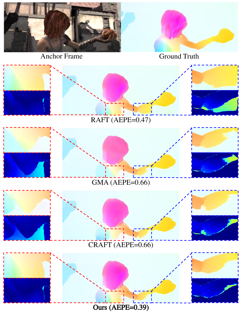
Figure 1. An example to show the superiority of our method. The estimated optical flow and the error map of different methods are visualized. Our method estimates less error and shows clear contours in the optical flow map.

Optical flow refers to the motion field between two frames, which is an important tool in computer vision and video processing. It has a wide range of application scenarios, including video super-resolution (Chan et al., 2022), video frame interpolation (Huang et al., 2022b), video inpainting (Xu et al., 2019), object detection (Li et al., 2018) and tracking (Vihlman and Visala, 2020), etc. In recent years, with the development of deep learning and neural networks, many high-performance deep learning optical flow estimation models have emerged. These models learn discriminative features and then utilize the feature correlation between two frames to estimate accurate optical flow. Although leaps and bounds have been made, the current optical flow estimation methods generally have a blind spot: they assume that the inputs are uncompressed high-quality frames, which is inconsistent with the practical situation. In fact, due to the huge amount of information, almost all videos are stored in a compressed format, which causes distortion and hinders the performance of existing optical flow models.

In order to find a solution, we need to look at the principles of video compression. The process of video compression can be divided into encoding and decoding. The basic idea of encoding is to dynamically divide the image into blocks and quantify them to discard the secondary information, thereby reducing the number of bits to store the video. Specifically, the compression algorithm also takes advantage of the video’s temporal continuity by matching the blocks of adjacent frames and sharing the information between frames to reduce redundancy further. The matching offsets are called motion vectors and are stored together in the compressed video. When decoding, the algorithm reads the encoded blocks with the motion vectors to reconstruct the image for each frame.

The motion vectors have a close definition to optical flow and can be regarded as a rough block-level optical flow. Importantly, it is already pre-computed and can be extracted from the compression code stream without additional computational cost. A simple way to use motion vectors is to use them directly as the initial solution for iterative optical flow models such as RAFT (Teed and Deng, 2020). However, we find that such an implementation fails to improve the accuracy of optical flow estimation. The main reason is that the existing deep optical flow models are better at handling smooth optical flow maps, while the sparse and block-level motion vectors do not fit this pattern and cannot be effectively utilized by those models. To exploit the motion vector prior, we propose our MVFlow with a Motion-Vector Converting Module (MVCM). The module can initially convert the domain of the motion vector map through the contextual correlation of the image, so that the motion information contained in motion vectors can be incorporated into the process of optical flow estimation. As shown in Figure 1, our MVFlow demonstrates excellent performance and estimates accurate motion for the arm and body in the area marked by the boxes.

Besides, we construct the training and evaluation datasets for optical flow estimation of compressed videos to conduct our experiments. We compress the videos of four typical optical flow datasets (FlyingThings 3D (Mayer et al., 2016), MPI Sintel(Butler et al., 2012) and KITTI 2012/2015 (Geiger et al., 2012; Menze and Geiger, 2015)) and extract the motion vectors from decoding.

In total, our contributions are:

• We propose a novel optical flow estimation framework that exploits video motion vectors as prior information for accurate and fast motion estimation for compressed videos. To the best of our knowledge, this is the first attempt that uses motion vectors to assist deep optical flow estimation.

• To address the domain gap between motion vectors and optical flow, we propose a Motion-Vector Converting Module that utilizes the correlation of video content and motion to regulate motion vectors.

• Experiments prove the superiority of MVFlow in terms of performance and efficiency. Compared to RAFT, MVFlow can reduce AEPE by 1.09 with the same iteration steps, or save 52% computation time to reach similar accuracy.

• For the first time, we construct four datasets containing optical flow, compressed frames and motion vectors of different compression qualities. We believe they can facilitate the research on optical flow estimation of compressed videos.

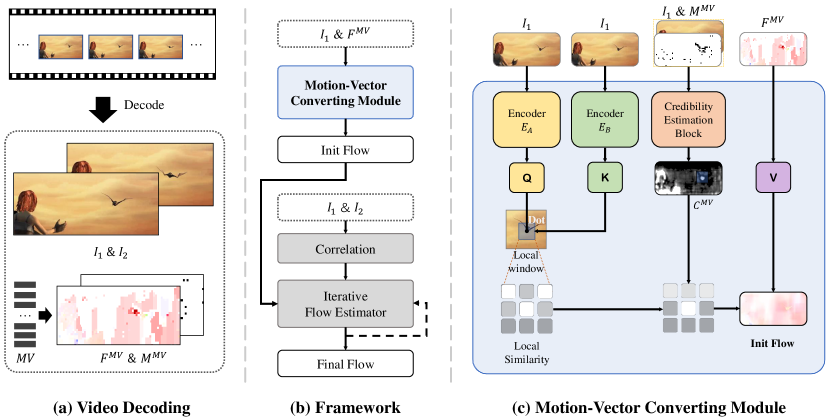
Figure 2. The architecture of our proposed MVFlow. (a) Decoding videos to get frames and the corresponding motion vectors. (b) The main framework of our MVFlow. (c) The structure of our Motion-Vector Converting Module.

2. Related Works

2.1. Optical Flow

Optical flow has been studied for a long time as a fundamental technology. Early on, according to the mathematical definition of optical flow, researchers design some traditional optical flow algorithms, such as Horn–Schunck (Horn and Schunck, 1981) and Lucas-Kanade (Lucas et al., 1981). These methods can effectively estimate the optical flow of simple cases, but their accuracy is generally not good.

With the advent of deep learning, researchers have also begun to use deep neural networks for optical flow estimation. FlowNet (Dosovitskiy et al., 2015) and FlowNet2.0 (Ilg et al., 2017) are the first attempt that proves the feasibility of deep learning in optical flow estimation. After that, the multi-scale models (Sun et al., 2018; Hui et al., 2018; Hur and Roth, 2019; Zhao et al., 2020) emerge. Next, RAFT (Teed and Deng, 2020) proposes an iterative method, which calculates global all-pair correlation and reuses it in every iteration. It has become the new baseline for subsequent researches. For example, various attention blocks (Sui et al., 2022; Zhao et al., 2022; Luo et al., 2022; Huang et al., 2022a) and big-kernel convolution layers (Sun et al., 2022) are added to the components of RAFT to provide stronger representation and estimation capabilities. Meanwhile, global motion aggregation (Jiang et al., 2021) and global matching (Xu et al., 2022; Zhao et al., 2022) are also proposed to break the over-dependence on local cues of models.

Recently, some works have also begun to study optical flow estimation under different degradation conditions. For example, Zhang et al. (Zhang et al., 2022) gives a solution to estimate optical flow in the dark, and Argaw et al. (Argaw et al., 2021) tries to estimate optical flow from a single motion-blurred image. For compressed video, Young et al. (Young et al., 2020) introduces compression prior information into traditional variational optimization for optical flow estimation. However, it is not comparable to deep learning methods in terms of accuracy and speed. To the best of our knowledge, we are the first to exploit compressed priors in deep optical flow estimation.

2.2. Video Compression

Video compression has become an indispensable part of video processing, which can effectively save storage and transmission bandwidth. In recent years, some deep learning-based video compression algorithms (Li et al., 2021; Lu et al., 2019; Yang et al., 2020; Hu et al., 2020) have been proposed with the expectation of achieving better compression performance. However, they are not currently available for practical applications due to the huge computational cost. Currently, commercial compression algorithms are still dominated by traditional methods(Wiegand et al., 2003; Sullivan et al., 2012; Bross et al., 2021).

Inter-frame predictive coding is an important part of traditional video compression algorithms. It calculates the motion vectors to measure the motion information between frames and removes temporal redundancy based on them. Note that motion vectors can be extracted from the compressed video stream without additional computational cost at the receiver end. Recently, some works attempt to utilize motion vectors to assist various vision tasks (Chen et al., 2021, 2020; Xu and Yao, 2022; Tan et al., 2020; Wu et al., 2018; Xu et al., 2016). Chen et al. (Chen et al., 2020) first explore the compressed video super-resolution task, and improve the model performance by leveraging the interactivity between decoding prior and deep prior. Specifically, they align the features of different frames based on motion vectors. Similarly, Xu et al. (Xu and Yao, 2022) uses motion vectors to propagate segmentation masks from keyframes to other frames, which can improve the efficiency and performance of video object segmentation. Considering that the motion vectors represent the primary motion of the videos, we use them to improve the performance of optical flow estimation in our work.

3. Proposed Method

In this section, we first analyze our motivations and then provide an overview of our optical flow estimation framework with motion vector prior. Next, the structure of our proposed MVCM is described in detail. Finally, we extend our MVCM to incorporate the common warm-start strategy.

3.1. Motivation

Almost all videos exposed to non-professional users are stored in a compressed format. The mainstream video compression frameworks perform motion compensation between frames, so the compressed video stores a set of offsets to represent the motion between frames. Such offsets are called motion vectors, which can be obtained without extra computational cost.

Motion vectors and optical flow are both representations of motion between frames, but there are two differences. Firstly, motion vectors are block-level, while optical flow records pixel-level motion. Second, motion vectors are calculated locally during encoding. It differs from the estimated optical flow, which needs to find motion field from the context of the entire frame. Therefore, using the motion vectors as an additional input can help optical flow estimation from two perspectives: 1) The optical flow model can conduct iterative updates based on the rough solution given by motion vectors, making converging faster. 2) Due to the distortion caused by compression, the inter-frame correspondence for some regions is disrupted, so the optical flow models rely more on the learned global prior like smoothness and ignores some small objects that move independently. In contrast, motion vectors store the best matches found for each block individually, which can play an important complementary role in estimating optical flow of compressed video.

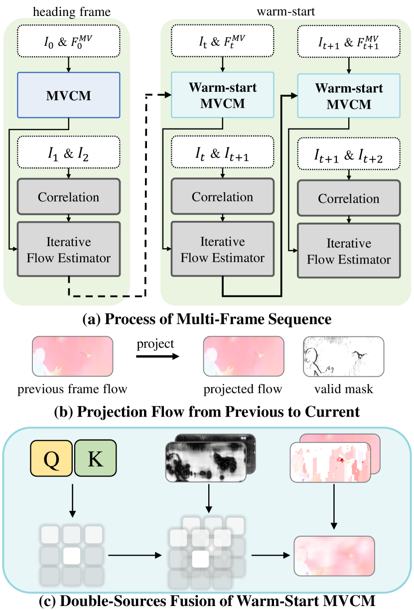
Figure 3. (a) Process of multi-frame sequence with warm-start strategy. For the heading frame, we use our ordinary MVCM, while for subsequent frames, we use warm-start MVCM, which can utilize the estimation of the previous frame. (b) Projection of flow from the previous frame to the current frame. (c) The modified aggregation process in warm-start MVCM.

3.2. Overview

As shown in Figure 2(a), we first decode the video to obtain consecutive frames and the corresponding motion vectors. We denote the first frame of the two frames as $I_{1}$, the second frame as $I_{2}$, and the motion vectors from the previous to the next frame as $MV$. The initial representation of $MV$ is a group of vectors, each of which records a compressed block’s position, size, and motion offset. We convert the $MV$ into a dense flow map denoted as $F^{MV}$ by filling the pixels in each block with the same motion offset. Subsequently, we estimate the optical flow with $F^{MV}$ as additional input in our framework shown in Figure 2(b). Our model is a variant based on RAFT (Teed and Deng, 2020), called MVFlow. The estimation process of MVFlow contains three stages, of which the first two stages can be parallelized. In the first stage, we adopt our Motion-Vector Converting Module to convert $F^{MV}$ into a smoother coarse flow map according to the contextual information of $I_{1}$. In the second stage, we extract the features of $I_{1}$ and $I_{2}$ and calculate the correlation. In the last stage, we take the converted coarse flow as the initial value and refer to the correlation information to perform an iterative optimization process.

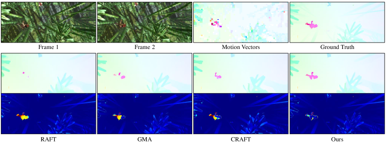
Figure 4. Qualitative comparison of our method and the state-of-the-art methods on Compressed Sintel. The displayed example is in QP of 37.

3.3. Motion-Vector Converting Module

The $F^{MV}$ obtained directly from the motion vectors has a large domain gap with the optical flow, which can not be utilized effectively by existing deep learning-based optical flow estimation architectures, as proved in our experiment (Section 4.4). Thus, we design a Motion-Vector Converting Module (MVCM) to convert $F^{MV}$ into the same domain of optical flow. Our inspiration consists of two parts. First, the $F^{MV}$ is sparse, and there are some regions without MV offsets, so we need to complement them with other regions. A good idea is to use the spatial correlation of $I_{1}$ to accomplish the filling process. Second, $F^{MV}$ also has some regions with inaccurate motion, which is caused by either the coarse block division or the matches not in line with actual motion. These wrong areas need to be figured out and corrected. We use the context information of $I_{1}$ to solve it. As a combination of the above two points, the specific design of our module is shown in Figure 2(c), which follows the attention mechanism. As Equation 1, $I_{1}$ is first fed into two different encoders to obtain Q and K maps, while $F^{MV}$ is directly taken as the V map, denoted as

(1) $$Q=E_{A}(I_{1}),~{}K=E_{B}(I_{1}),~{}V=F^{MV}$$

$E_{A}$ and $E_{B}$ are two encoder blocks, each consisting of six convolution and corresponding activation layers. Then, in order to find the areas that need to be corrected, we use a Credibility Estimation Block to estimate the credibility of the motion prior for each pixel. This can be expressed as

(2) $$C^{MV}=CEB(I_{1},{M}^{MV})$$

where $M^{MV}$ refers to a mask indicating which regions have motion vectors, $C^{MV}$ is a weight map in the range $(0,1)$, and $CEB$ is a CNN block, which contains six convolution layers, six dilation convolution layers and their corresponding activation layers. The dilation convolution layers can extract broader contextual information to utilize spatial information comprehensively. The last activation function is sigmoid for limiting the range of $C^{MV}$. We perform the correlation computation in local sliding windows instead of all pixels to avoid introducing too much extra computation. First, the correlation between the center pixel of the local window and other pixels is calculated:

(3) $$S_{i,j}=softmax(Q_{i,j}\cdot K_{i+k,j+l}),$$

where $k,l\in[-d,d]$. The $\cdot$ mark refers to the vector dot product operator, so the computed correlation weight $S_{i,j}$ is a tensor of shape $(2d+1)^{2}$. Then the credibility of the pixels is combined with the correlation to get the final weights, donated as:

(4) $$W^{MV}_{i,j}=S_{i,j}\odot\hat{C}^{MV}_{i,j}$$

The $\hat{C}^{MV}_{i,j}$ is a (2d+1)$\times$(2d+1) window extracted from $C^{MV}$ around pixel $(i,j)$. The $\odot$ mark refers to the element-wise product operator. At last, we aggregate motions in local windows with the calculated weights:

(5) $$F_{i,j}=\frac{\sum_{k,l}{W^{MV}_{i,j,k,l}V_{i+k,j+l}}}{\sum_{k,l}{W^{MV}_{i,j,k,l}}}$$

3.4. Combination with Warm-Start Strategy

In the practical setting for iterative optical flow estimation, a well-known strategy called warm-start uses the optical flow predicted for the previous frame as initialization, shown in Figure 3(a). Our method also provides an initialization from motion vectors. Therefore, to simultaneously utilize these two different sources of optical flow initialization, we design a warm-start MVCM module to fuse them. First, as shown in Figure 3(b), we need to project the flow of the previous frame to the current frame:

(6) $$F^{Prj}=FW(F^{Pre},F^{Pre}),~{}M^{Prj}=FW(O,F^{Pre})$$

$F^{Pre}$ is the flow estimation of the previous frame, and $F^{Prj}$ is the projected flow. $FW$ refers to forward warping, which will cause holes and overlaps. Thus, we calculate the valid mask $M^{Prj}$ of $F^{Prj}$ by forward warp an all-one matrix $O$.

Then, we send $M^{Prj}$, $M^{MV}$ and $I_{1}$ to a modified Credibility Estimation Block denoted as $CEB^{{}^{\prime}}$, and get two credibility maps $C^{Prj}$ and $C^{MV}$, corresponding to $F^{Prj}$ and $F^{MV}$ respectively, denoted as

(7) $$C^{Prj},C^{MV}=CEB^{{}^{\prime}}(I_{1},M^{MV},M^{Prj})$$

Next, as shown in Figure 3(c), we calculate the weights of projected flow as Equation 4 and 8.

(8) $$W^{Prj}_{i,j}=S_{i,j}\odot\hat{C}^{Prj}_{i,j}$$

Finally, we replace Equation 5 with Equation 9, which means a fusion of the two different sources of initialization.

(9) $$F_{i,j}=\frac{\sum_{k,l}{W^{MV}_{i,j,k,l}V^{MV}_{i+k,j+l}+W^{Prj}_{i,j,k,l}V^{Prj}_{i+k,j+l}}}{\sum_{k,l}{W^{MV}_{i,j,k,l}+W^{Prj}_{i,j,k,l}}},$$

where $V^{MV}$ and $V^{Prj}$ correspond to $F^{MV}$ and $F^{Prj}$ respectively.

Table 1. Comparison of our method and three well-known optical flow methods. We adopt AEPE and F1 as the metrics for all datasets, and both are lower when the results are more accurate. For each QP setting, we color the best value for each column in red.

QP	Method	MPI Sintel				KITTI 2012				KITTI 2015
		clean pass		final pass		NOC		ALL		NOC		ALL
		AEPE	F1	AEPE	F1	AEPE	F1	AEPE	F1	AEPE	F1	AEPE	F1
22	RAFT	1.90	6.09%	3.48	11.58%	1.34	7.01%	2.78	13.50%	3.13	12.96%	6.54	21.19%
	GMA	2.07	6.11%	4.43	13.37%	1.45	7.85%	2.68	14.09%	3.45	14.30%	6.74	21.92%
	CRAFT	1.95	7.41%	3.95	13.32%	1.50	8.27%	2.79	14.67%	3.60	14.94%	6.59	22.66%
	GMFlow	1.66	5.75%	3.86	12.59%	1.79	9.29%	3.47	15.81%	3.31	15.68%	6.91	23.19%
	GMFlowNet	2.13	8.29%	4.22	14.71%	1.34	6.69%	2.68	12.57%	2.85	11.68%	5.97	19.26%
	Ours	1.85	5.56%	3.43	10.27%	1.29	6.58%	2.59	12.60%	3.13	12.80%	6.07	20.64%
27	RAFT	2.16	6.87%	3.79	12.75%	1.51	8.62%	3.03	15.27%	3.43	14.59%	7.00	22.79%
	GMA	2.16	6.83%	3.25	9.95%	1.76	9.80%	3.12	16.05%	3.89	15.87%	7.41	23.40%
	CRAFT	2.07	8.06%	4.20	14.40%	1.73	10.24%	3.15	16.60%	3.84	16.64%	7.29	24.36%
	GMFlow	1.89	6.48%	4.09	13.92%	2.03	11.01%	3.84	17.71%	3.77	17.54%	7.66	24.91%
	GMFlowNet	2.48	9.43%	4.46	16.15%	1.59	8.49%	3.11	14.54%	3.34	13.37%	6.79	20.84%
	Ours	2.01	6.20%	3.70	11.28%	1.41	7.97%	2.83	14.20%	3.17	13.98%	6.25	21.82%
32	RAFT	2.54	8.27%	4.06	14.74%	2.14	12.77%	3.94	19.64%	4.69	18.81%	8.89	26.60%
	GMA	2.45	8.49%	4.53	16.95%	2.16	13.13%	3.68	19.63%	4.83	19.99%	8.88	27.21%
	CRAFT	2.48	9.83%	4.46	16.66%	2.16	13.86%	3.79	20.57%	4.63	20.73%	8.61	28.27%
	GMFlow	2.12	8.29%	4.42	16.07%	2.50	14.46%	4.57	21.35%	4.70	21.55%	9.13	28.75%
	GMFlowNet	2.91	11.45%	4.90	18.63%	2.28	12.80%	4.07	19.18%	4.46	17.73%	8.59	25.14%
	Ours	2.24	7.47%	4.01	13.22%	1.88	11.58%	3.48	18.19%	4.09	17.62%	7.66	25.30%
37	RAFT	3.09	15.14%	4.95	18.35%	3.06	19.46%	5.31	26.37%	6.29	24.85%	11.33	32.12%
	GMA	3.18	11.93%	4.80	19.38%	2.91	18.85%	4.76	25.35%	6.63	25.62%	11.61	32.36%
	CRAFT	3.16	13.39%	5.27	20.40%	3.10	20.77%	5.13	27.37%	6.41	26.94%	11.30	34.08%
	GMFlow	2.77	11.79%	4.96	18.78%	3.37	20.42%	5.91	27.49%	6.04	26.89%	11.22	33.74%
	GMFlowNet	3.61	14.83%	5.51	21.92%	3.20	19.21%	5.34	25.72%	6.23	24.57%	11.01	31.37%
	Ours	2.87	10.57%	4.80	17.06%	2.86	18.74%	4.92	25.14%	5.19	23.28%	9.43	30.52%

4. Experiments

4.1. Dataset Construction

We make our compressed video optical flow dataset based on four existing datasets. They are: FlyingThings3D(Mayer et al., 2016), MPI Sintel(train) (Butler et al., 2012), KITTI 2012(train) (Geiger et al., 2012) and KITTI 2015(train) (Menze and Geiger, 2015). In our experiments, we use the H264 codec to compress the video because H264 is currently the most mature and widely used encoding tool. We first encode each sequence in the dataset with four different quantization parameters, 22, 27, 32, and 37. In order to maintain the consistency of the direction of motion vectors and optical flow, the videos are compressed in reverse order. Then, each frame and the corresponding motion vectors are decoded from the compressed videos. In the experiment, we use the Compressed FlyingThings3D as the training set, and the rest datasets are set as the evaluation benchmark. All the generated datasets will be uploaded to the public platform to facilitate future research.

4.2. Settings

We implement our model based on the code of RAFT(Teed and Deng, 2020). The loss functions are added to all the intermediate flow estimations (including the output of MVCM) and trained the model for 120k steps on the aforementioned Compressed FlyingThings dataset. We use only four iterations in each step to speed up the training. We use AdamW (Loshchilov and Hutter, 2019) optimizer and set weight_decay=5e-5 and eps=1e-8. The learning rate is set to 1e-4 and decays linearly to 8.5e-5 during training. The batch_size is set to 4. Our training device is a single Nvidia RTX 3090. For data augmentation, we randomly crop 800$\times$512 patches of the input frames for training. For better convergence, we use the original RAFT parameters on FlyingThings as the initialization parameters of those unmodified layers. At the same time, in order to train our model with the warm-start strategy, we fine-tune our model for an additional 30k steps, and the original MVCM parameters are fixed during fine-tuning. Other models for comparison that emerged in the experiments follow the same training process. Unless otherwise stated, all models are evaluated with 16 iterations.

Table 2. Ablation Study of four models, including the baseline model, the retrained model, the retrained model with MV inputs and our final model with MVCM. We also provide results on Compressed MPI Sintel and Compressed KITTI 2012 in the supplementary material.

QP	Method	Compressed KITTI 2015
		NOC		ALL
		AEPE	F1	AEPE	F1
22	Baseline	4.34	16.72%	10.07	25.58%
	$\uparrow$ + Retrain	3.13	12.96%	6.54	21.19%
	$\uparrow$ + MV	3.48	13.39%	6.98	21.61%
	$\uparrow$ + MVCM	3.13	12.80%	6.07	20.64%
27	Baseline	5.22	19.79%	11.53	28.34%
	$\uparrow$ + Retrain	3.43	14.59%	7.00	22.79%
	$\uparrow$ + MV	3.63	14.93%	7.36	23.07%
	$\uparrow$ + MVCM	3.17	13.98%	6.25	21.82%
32	Baseline	7.36	27.13%	14.53	34.74%
	$\uparrow$ + Retrain	4.69	18.81%	8.89	26.60%
	$\uparrow$ + MV	4.90	19.27%	9.27	27.02%
	$\uparrow$ + MVCM	4.09	17.62%	7.66	25.30%
37	Baseline	9.67	35.58%	17.52	42.11%
	$\uparrow$ + Retrain	6.29	24.85%	11.33	32.12%
	$\uparrow$ + MV	6.55	25.38%	11.80	32.57%
	$\uparrow$ + MVCM	5.19	23.28%	9.43	30.52%

4.3. Comparison with the State-of-the-Art Methods

We first compare our MVFlow with five well-known optical flow methods. They are RAFT(Teed and Deng, 2020), GMA(Jiang et al., 2021), CRAFT(Sui et al., 2022), GMFlow(Xu et al., 2022) (GMF) and GMFlowNet(Zhao et al., 2022) (GMFNet). Because off-the-shelf optical flow models do not perform well on compressed video (as shown in Supplementary Materials), all models are retrained with the same settings as ours. AEPE (Average Endpoint Error) and F1 (percentage of outliers) are chosen as metrics in our experiment. The results are shown in Tab 1. As we can see, in the vast majority of comparisons, our method shows clear superiority.

An interesting pattern is that although the performance of RAFT, GMA, and CRAFT is progressively improved on the uncompressed optical flow test set, CRAFT and GMA do not outperform RAFT in compressed videos. This may be due to the lack of flexibility caused by the large amount of attention computation introduced by GMA and CRAFT.

We can also find that our method leads by a more significant margin at a higher QP. The reason is that higher QP introduces more compression noise, making motion estimation more challenging. Despite retraining on Compressed FlyingThings, RAFT, GMA and CRAFT still fail to find correct motion from the compressed videos. Unlike them, our method can handle this situation by exploiting the motion vectors.

We also give an example for qualitative comparison in Figure 4, which are from Compressed Sintel dataset. The methods without utilizing motion vectors fail to estimate the flow of the human in the first example and the window in the second example. With motion vectors as additional hints, our method generates finer initializations, thus better handling these complex cases. The example from KITTI 2015 dataset can be found in the appendix.

Figure 5. The comparison of our MVFlow and the retrained RAFT on a group of frames with different QP. RAFT produces various wrong estimates due to information loss during video compression, while our model, while our model shows robustness on different QP.

Table 3. Comparison of different initialization strategies.

QP	Method	Compressed MPI Sintel
		clean pass		final pass
		AEPE	F1	AEPE	F1
22	Zero	1.90	6.09%	3.48	11.58%
	Warm-Start	1.83	6.12%	3.46	11.37%
	MVCM	1.85	5.56%	3.43	10.27%
	MVCM + Warm-Start	1.71	5.71%	3.28	10.64%
27	Zero	2.16	6.87%	3.79	12.75%
	Warm-Start	2.01	6.86%	3.58	12.58%
	MVCM	2.01	6.20%	3.70	11.28%
	MVCM + Warm-Start	1.80	6.40%	3.50	11.74%
32	Zero	2.54	8.27%	4.06	14.74%
	Warm-Start	2.33	8.30%	4.05	14.78%
	MVCM	2.24	7.47%	4.01	13.22%
	MVCM + Warm-Start	2.11	7.74%	3.94	13.88%
37	Zero	3.09	15.14%	4.95	18.35%
	Warm-Start	3.17	11.67%	4.91	18.46%
	MVCM	2.87	10.57%	4.80	17.06%
	MVCM + Warm-Start	2.86	10.71%	4.43	17.39%

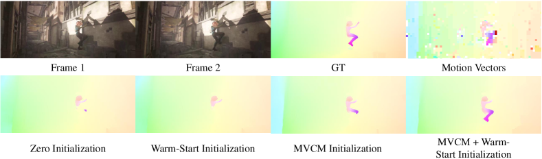
Figure 6. A group of qualitative examples of different initialization methods.

4.4. Ablation Study

We design a set of ablation experiments to probe the effect of each of our modifications. A total of four models are compared in the experiment, and the results can be found in Table 6. The first model is the baseline, which directly uses the pre-trained parameters of RAFT (raft-things.pth). The second model is retrained on our Compressed FlyingThings and is thus more robust to compression noise. The third model simply adds motion vectors for initialization based on the second model. Experiments show that this naive scheme brings negative lift. The last model, our full MVFlow, adds MVCM as a preprocessing module, which converts the motion vectors to the same domain of optical flow. We can see in the table that MVCM brings a significant improvement. To show the effectiveness and robustness of our proposed method, we give qualitative comparisons on different QP settings in Figure 5.

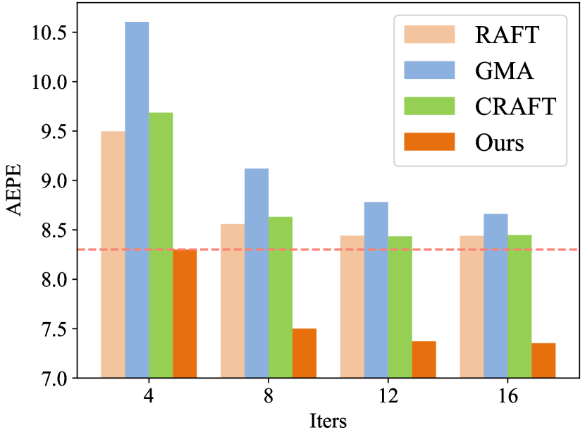
Figure 7. Efficiency comparison of four methods on Compressed KITTI 2015 dataset. The red dashed line highlights the performance of our method with four iterations

4.5. Discussion

Warm-Start Strategy As mentioned in Section 3.4, warm-start is a common strategy used in iterative optical flow estimation methods for videos. It has a commonality with our method, that is, both of them give an initialized flow estimation for iteration. We evaluate four settings on Compressed MPI Sintel dataset to compare different initialization methods. They are the model with zero initialization, the model with warm-start initialization, the model with our MV initialization, and the model with combined strategy introduced in Section 3.4. The results are shown in Table 3, from where we can find that our combined strategy gets the best AEPE score, and our initialization gets the best F1 score. This means that the combined strategy brings an overall improvement compared to only using motion vectors, but the robustness to some problematic areas is reduced. Overall, both of our initialization strategies outperform the simple warm-start strategy. Figure 6 gives qualitative examples of different initialization methods. The motion vectors provide clear guidelines for the movement of the character’s leg, thus enabling fine-grained optical flow estimation.

Computational Efficiency We compare the accuracy of different models with different iteration steps and give the result in Figure 7 and Table 4. It can be clearly seen that our model only needs four iterations to outperform the results of other models with 16 iterations. This means that our model has a vast efficiency advantage under the requirement of achieving the same accuracy. Specifically, on an Nvidia RTX 3090, RAFT takes an average of 91ms to perform 16 iterations. In comparison, our method only needs four iterations that take 44ms to achieve comparable results, saving 52% of computation time, which brings many benefits for practical use. On the other hand, our method outperforms RAFT by 1.09 of AEPE under the same iteration steps with only a slight increase in runtime.

Table 4. Running time required to achieve similar accuracy. Meanwhile, the performance under the same iterations is shown in the last column.

	RAFT	GMA	CRAFT	GMF	GMFNet	Ours	(Ours)
Iterations	16	16	16	-	16	4	16
Runtime	91ms	119ms	362ms	125ms	174ms	44ms	99ms
$\Delta$ Runtime	-0%	+31%	+298%	+37%	+91%	-52%	+9%
AEPE	8.44	8.66	8.45	8.73	8.09	8.30	7.35
$\Delta$ AEPE	-0.00	+0.22	+0.01	+0.29	-0.35	-0.14	-1.09

5. Conclusion

Optical flow estimation is an essential technique in the field of computer vision and video processing. However, almost all the videos are compressed. Existing methods ignore the powerful compression prior, thus fail to handle frames with compression noise. In this paper, we introduce the motion vectors in the compressed video stream to optical flow estimation. Our proposed MVFlow contains a Motion-Vector Converting Module to convert the motion vectors to the same domain of optical flow to better estimate the optical flow. We also construct four optical flow datasets for compressed videos. The experiments show that our proposed method is superior in effectiveness and efficiency.

Appendix A Qualitative comparison on KITTI 2015

We supplement a set of visual comparisons on Compressed KITTI 2015 in Figure 8, where our method estimates a more complete optical flow map.

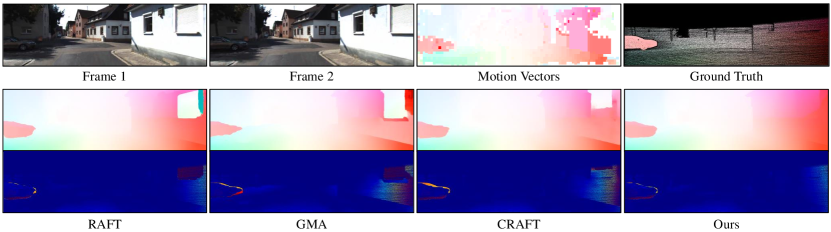
Figure 8. Qualitative comparison on Compressed KITTI 2015.

A.1. The Necessity of Retraining the State-of-the-art Models

As mentioned in the main manuscript, the off-the-shelf optical flow estimation models are not trained with compressed videos. Thus it cannot handle the compression noise well. For a fair comparison, we need to fine-tune the state-of-the-art model using the compressed data and settings the same as Ours. Table 5 shows the comparisons of RAFT (Teed and Deng, 2020), GMA(Jiang et al., 2021), CRAFT(Sui et al., 2022), GMFlow(Xu et al., 2022) and GMFlowNet(Zhao et al., 2022). The fine-tuning improves the performance of these methods for optical flow estimation on compressed videos, removing the influence of different training data and strengthening our experiments’ rigor. The only exception is that GMFlowNet’s performance on Compressed MPI Sintel decreased slightly after fine-tune, which may be due to the complex POLA structure and the Global Matching operation of GMFlowNet are sensitive to the distribution difference between Compressed Things and compressed MPI Sintel. However, GMFlowNet shows a very significant performance improvement on Compressed KITTI 2015 after fine-tuning, which still proves the role of retraining.

Table 5. The performance of state-of-the-art methods before and after fine-tuning. We test on two datasets including Compreesed MPI Sintel and Compressed KITTI 2015. The values given are the average test results on all QPs (22, 27,32,37).

Method	Compressed MPI Sintel				Compressed KITTI 2015
	clean pass		final pass		NOC		ALL
	AEPE	F1	AEPE	F1	AEPE	F1	AEPE	F1
RAFT	2.98	10.51%	5.09	18.14%	6.65	24.81%	10.07	25.58%
RAFT-ft	2.42	8.19%	4.07	14.36%	4.38	17.80%	8.44	25.67%
GMA	2.52	9.68%	4.58	17.87%	5.48	21.00%	9.95	27.96%
GMA-ft	2.46	8.34%	4.09	14.80%	4.70	18.95%	8.66	26.22%
CRAFT	2.39	9.43%	4.42	17.34%	5.56	20.89%	9.91	27.70%
CRAFT-ft	2.10	8.08%	3.86	11.33%	4.62	18.62%	8.55	25.94%
GMFlow	2.64	10.58%	4.94	19.24%	5.93	24.53%	11.45	31.49%
GMFlow-ft	2.11	8.08%	4.33	15.34%	4.46	20.41%	8.73	27.65%
GMFlowNet	2.48	9.27%	4.72	16.82%	5.58	20.97%	10.29	27.68%
GMFlowNet-ft	2.78	11.00%	4.78	17.85%	4.22	16.84%	8.09	24.15%

Appendix B Full Ablation Study on Three Datasets

Due to the limited number of pages, we only give the results of the ablation experiment on Compressed KITTI 2015 in the main manuscript. Here, we present the complete ablation experiments on three datasets in Table 6. Similar to the results on Compressed KITTI 2015, the retraining and our proposed MVCM bring significant improvements. Using MV directly as initialization brings slight improvement on Compressed MPI Sintel, and even slightly hurts the performance on Compressed KITTI 2012/2015, further proving the necessity and effectiveness of our proposed MVCM.

Table 6. Complete ablation study on three datasets.

QP	Method	Compressed MPI Sintel				Compressed KITTI 2012				Compressed KITTI 2015
		clean pass		final pass		NOC		ALL		NOC		ALL
		AEPE	F1	AEPE	F1	AEPE	F1	AEPE	F1	AEPE	F1	AEPE	F1
22	Baseline	2.07	6.19%	3.99	12.62%	1.93	9.21%	4.98	18.18%	4.34	16.72%	10.07	25.58%
	$\uparrow$ + Retrain	1.90	6.09%	3.48	11.58%	1.34	7.01%	2.78	13.50%	3.13	12.96%	6.54	21.19%
	$\uparrow$ + MV	1.90	6.04%	3.48	11.14%	1.36	7.03%	2.82	13.52%	3.48	13.39%	6.98	21.61%
	$\uparrow$ + MVCM	1.85	5.56%	3.43	10.27%	1.29	6.58%	2.59	12.60%	3.13	12.80%	6.07	20.64%
27	Baseline	2.40	7.76%	4.44	15.42%	2.52	14.04%	5.85	22.70%	5.22	19.79%	11.53	28.34%
	$\uparrow$ + Retrain	2.16	6.87%	3.79	12.75%	1.51	8.62%	3.03	15.27%	3.43	14.59%	7.00	22.79%
	$\uparrow$ + MV	2.13	6.82%	3.77	12.38%	1.57	8.76%	3.14	15.40%	3.63	14.93%	7.36	23.07%
	$\uparrow$ + MVCM	2.01	6.20%	3.70	11.28%	1.41	7.97%	2.83	14.20%	3.17	13.98%	6.25	21.82%
32	Baseline	3.02	11.10%	5.32	19.54%	3.94	21.79%	7.83	29.86%	7.36	27.13%	14.53	34.74%
	$\uparrow$ + Retrain	2.54	8.27%	4.06	14.74%	2.14	12.77%	3.94	19.64%	4.69	18.81%	8.89	26.60%
	$\uparrow$ + MV	2.43	8.26%	4.10	14.71%	2.18	12.91%	4.03	19.78%	4.90	19.27%	9.27	27.02%
	$\uparrow$ + MVCM	2.24	7.47%	4.01	13.22%	1.88	11.58%	3.48	18.19%	4.09	17.62%	7.66	25.30%
37	Baseline	4.44	16.97%	6.59	25.00%	5.47	32.69%	9.88	39.93%	9.67	35.58%	17.52	42.11%
	$\uparrow$ + Retrain	3.09	15.14%	4.95	18.35%	3.06	19.46%	5.31	26.37%	6.29	24.85%	11.33	32.12%
	$\uparrow$ + MV	3.10	11.51%	5.00	18.55%	3.26	19.95%	5.67	26.81%	6.55	25.38%	11.80	32.57%
	$\uparrow$ + MVCM	2.87	10.57%	4.80	17.06%	2.86	18.74%	4.92	25.14%	5.19	23.28%	9.43	30.52%

Appendix C More Discussion

C.1. Validation on Clean Frames

For direct comparison with off-the-shelf optical flow models and further verifying the effect of our MVCM, we also test the performance of our model on clean frames. Our settings are consistent with RAFT, and the motion vectors under QP 22 (with the highest quality) are added as the input of MVCM. As shown in Table 7, our model can outperform the baseline RAFT on both the Sintel and KITTI datasets. At the same time, we also submitted our test results on Sintel and KTTI benchmarks and achieved performance beyond RAFT.

C.2. Assisting Downstream Tasks

Accurate alignment is critical in video processing tasks. We design an experiment to demonstrate that our method can provide better alignments for downstream tasks. The experiment uses a composite task: given two compressed frames, use a U-Net model to synthesize the denoised two frames and the intermediate frame. The input of U-Net contains the original and the warped frames. In our comparison, the U-Net structure remains unchanged, and we only replace the optical flow used in warping. We choose QP 37 in this experiment because it is the most common in practice. The results are shown in Table 8, which shows that the optical flow estimated by our method is more suitable for assisting compression video-related tasks.

C.3. Validation on HEVC Codec

To verify the flexibility of our method, we add an experiment with HEVC(H.265) codec. We adopt HEVC official lowdelay P coding settings, and set the reference frame to the previous frame (-1). We conduct the experiments on the clean pass of Sintel datasets with QP 32. As shown in Table 9, our method is able to work well for other codecs, which demonstrates the generalization performance of our method.

Table 7. Comparison on clean optical flow datasets.

Train Data	C+T				C+T+S+K(+H)
Method	Sintel(val)		KITTI(val)		Sintel(test)		KITTI(test)
RAFT	1.43	2.71	5.04	17.40	1.61	2.86	5.10
Ours	1.38	2.67	4.66	17.02	1.53	2.71	4.90

Table 8. Comparison on downstream tasks. DF means denoised frames, and IF means interpolated frames. The experiment is taken on Vimeo-90K (Xue et al., 2019) dataset.

Model	DF PSNR	DF SSIM	IF PSNR	IF SSIM
RAFT + UNet	26.05	0.8480	24.94	0.8266
Ours + Unet	26.31	0.8517	25.18	0.8365

Table 9. The additional verification experiment on HEVC codec.

Model	AEPE	F1
Baseline(RAFT)	2.50	8.71
Ours-MVFlow	2.40	7.89

References

- (1)
- Argaw et al. (2021) Dawit Mureja Argaw, Junsik Kim, Francois Rameau, Jae Won Cho, and In So Kweon. 2021. Optical flow estimation from a single motion-blurred image. In Proceedings of the AAAI Conference on Artificial Intelligence, Vol. 35. 891–900.
- Bross et al. (2021) Benjamin Bross, Jianle Chen, Jens-Rainer Ohm, Gary J Sullivan, and Ye-Kui Wang. 2021. Developments in international video coding standardization after avc, with an overview of versatile video coding (vvc). Proc. IEEE 109, 9 (2021), 1463–1493.
- Butler et al. (2012) Daniel J Butler, Jonas Wulff, Garrett B Stanley, and Michael J Black. 2012. A naturalistic open source movie for optical flow evaluation. In European conference on computer vision. Springer, 611–625.
- Chan et al. (2022) Kelvin CK Chan, Shangchen Zhou, Xiangyu Xu, and Chen Change Loy. 2022. BasicVSR++: Improving video super-resolution with enhanced propagation and alignment. In Proceedings of the IEEE/CVF Conference on Computer Vision and Pattern Recognition. 5972–5981.
- Chen et al. (2020) Peilin Chen, Wenhan Yang, Long Sun, and Shiqi Wang. 2020. When bitstream prior meets deep prior: Compressed video super-resolution with learning from decoding. In Proceedings of the 28th ACM International Conference on Multimedia. 1000–1008.
- Chen et al. (2021) Peilin Chen, Wenhan Yang, Meng Wang, Long Sun, Kangkang Hu, and Shiqi Wang. 2021. Compressed Domain Deep Video Super-Resolution. IEEE Transactions on Image Processing 30 (2021), 7156–7169.
- Dosovitskiy et al. (2015) Alexey Dosovitskiy, Philipp Fischer, Eddy Ilg, Philip Hausser, Caner Hazirbas, Vladimir Golkov, Patrick Van Der Smagt, Daniel Cremers, and Thomas Brox. 2015. Flownet: Learning optical flow with convolutional networks. In Proceedings of the IEEE international conference on computer vision. 2758–2766.
- Geiger et al. (2012) Andreas Geiger, Philip Lenz, and Raquel Urtasun. 2012. Are we ready for autonomous driving? the kitti vision benchmark suite. In 2012 IEEE conference on computer vision and pattern recognition. IEEE, 3354–3361.
- Horn and Schunck (1981) Berthold KP Horn and Brian G Schunck. 1981. Determining optical flow. Artificial intelligence 17, 1-3 (1981), 185–203.
- Hu et al. (2020) Zhihao Hu, Zhenghao Chen, Dong Xu, Guo Lu, Wanli Ouyang, and Shuhang Gu. 2020. Improving deep video compression by resolution-adaptive flow coding. In European Conference on Computer Vision. Springer, 193–209.
- Huang et al. (2022a) Zhaoyang Huang, Xiaoyu Shi, Chao Zhang, Qiang Wang, Ka Chun Cheung, Hongwei Qin, Jifeng Dai, and Hongsheng Li. 2022a. Flowformer: A transformer architecture for optical flow. In European Conference on Computer Vision. Springer, 668–685.
- Huang et al. (2022b) Zhewei Huang, Tianyuan Zhang, Wen Heng, Boxin Shi, and Shuchang Zhou. 2022b. Real-time intermediate flow estimation for video frame interpolation. In European Conference on Computer Vision. Springer, 624–642.
- Hui et al. (2018) Tak-Wai Hui, Xiaoou Tang, and Chen Change Loy. 2018. Liteflownet: A lightweight convolutional neural network for optical flow estimation. In Proceedings of the IEEE conference on computer vision and pattern recognition. 8981–8989.
- Hur and Roth (2019) Junhwa Hur and Stefan Roth. 2019. Iterative residual refinement for joint optical flow and occlusion estimation. In Proceedings of the IEEE/CVF Conference on Computer Vision and Pattern Recognition. 5754–5763.
- Ilg et al. (2017) Eddy Ilg, Nikolaus Mayer, Tonmoy Saikia, Margret Keuper, Alexey Dosovitskiy, and Thomas Brox. 2017. Flownet 2.0: Evolution of optical flow estimation with deep networks. In Proceedings of the IEEE conference on computer vision and pattern recognition. 2462–2470.
- Jiang et al. (2021) Shihao Jiang, Dylan Campbell, Yao Lu, Hongdong Li, and Richard Hartley. 2021. Learning to estimate hidden motions with global motion aggregation. In Proceedings of the IEEE/CVF International Conference on Computer Vision. 9772–9781.
- Li et al. (2018) Guanbin Li, Yuan Xie, Tianhao Wei, Keze Wang, and Liang Lin. 2018. Flow guided recurrent neural encoder for video salient object detection. In Proceedings of the IEEE conference on computer vision and pattern recognition. 3243–3252.
- Li et al. (2021) Jiahao Li, Bin Li, and Yan Lu. 2021. Deep contextual video compression. Advances in Neural Information Processing Systems 34 (2021), 18114–18125.
- Loshchilov and Hutter (2019) Ilya Loshchilov and Frank Hutter. 2019. Decoupled weight decay regularization. In International Conference on Learning Representations.
- Lu et al. (2019) Guo Lu, Wanli Ouyang, Dong Xu, Xiaoyun Zhang, Chunlei Cai, and Zhiyong Gao. 2019. Dvc: An end-to-end deep video compression framework. In Proceedings of the IEEE/CVF Conference on Computer Vision and Pattern Recognition. 11006–11015.
- Lucas et al. (1981) Bruce D Lucas, Takeo Kanade, et al. 1981. An iterative image registration technique with an application to stereo vision. In Proceedings of the 7th International Joint Conference on Artificial Intelligence, Vol. 2. 674–679.
- Luo et al. (2022) Ao Luo, Fan Yang, Xin Li, and Shuaicheng Liu. 2022. Learning Optical Flow With Kernel Patch Attention. In Proceedings of the IEEE/CVF Conference on Computer Vision and Pattern Recognition (CVPR). 8906–8915.
- Mayer et al. (2016) Nikolaus Mayer, Eddy Ilg, Philip Hausser, Philipp Fischer, Daniel Cremers, Alexey Dosovitskiy, and Thomas Brox. 2016. A large dataset to train convolutional networks for disparity, optical flow, and scene flow estimation. In Proceedings of the IEEE conference on computer vision and pattern recognition. 4040–4048.
- Menze and Geiger (2015) Moritz Menze and Andreas Geiger. 2015. Object scene flow for autonomous vehicles. In Proceedings of the IEEE conference on computer vision and pattern recognition. 3061–3070.
- Sui et al. (2022) Xiuchao Sui, Shaohua Li, Xue Geng, Yan Wu, Xinxing Xu, Yong Liu, Rick Goh, and Hongyuan Zhu. 2022. CRAFT: Cross-Attentional Flow Transformer for Robust Optical Flow. In Proceedings of the IEEE/CVF Conference on Computer Vision and Pattern Recognition. 17602–17611.
- Sullivan et al. (2012) Gary J Sullivan, Jens-Rainer Ohm, Woo-Jin Han, and Thomas Wiegand. 2012. Overview of the high efficiency video coding (HEVC) standard. IEEE Transactions on circuits and systems for video technology 22, 12 (2012), 1649–1668.
- Sun et al. (2018) Deqing Sun, Xiaodong Yang, Ming-Yu Liu, and Jan Kautz. 2018. Pwc-net: Cnns for optical flow using pyramid, warping, and cost volume. In Proceedings of the IEEE conference on computer vision and pattern recognition. 8934–8943.
- Sun et al. (2022) Shangkun Sun, Yuanqi Chen, Yu Zhu, Guodong Guo, and Ge Li. 2022. Skflow: Learning optical flow with super kernels. Advances in Neural Information Processing Systems 35 (2022), 11313–11326.
- Tan et al. (2020) Zhentao Tan, Bin Liu, Qi Chu, Hangshi Zhong, Yue Wu, Weihai Li, and Nenghai Yu. 2020. Real time video object segmentation in compressed domain. IEEE Transactions on Circuits and Systems for Video Technology 31, 1 (2020), 175–188.
- Teed and Deng (2020) Zachary Teed and Jia Deng. 2020. Raft: Recurrent all-pairs field transforms for optical flow. In European conference on computer vision. Springer, 402–419.
- Vihlman and Visala (2020) Mikko Vihlman and Arto Visala. 2020. Optical flow in deep visual tracking. In Proceedings of the AAAI Conference on Artificial Intelligence, Vol. 34. 12112–12119.
- Wiegand et al. (2003) Thomas Wiegand, Gary J Sullivan, Gisle Bjontegaard, and Ajay Luthra. 2003. Overview of the H. 264/AVC video coding standard. IEEE Transactions on circuits and systems for video technology 13, 7 (2003), 560–576.
- Wu et al. (2018) Chao-Yuan Wu, Manzil Zaheer, Hexiang Hu, R Manmatha, Alexander J Smola, and Philipp Krähenbühl. 2018. Compressed video action recognition. In Proceedings of the IEEE conference on computer vision and pattern recognition. 6026–6035.
- Xu et al. (2022) Haofei Xu, Jing Zhang, Jianfei Cai, Hamid Rezatofighi, and Dacheng Tao. 2022. Gmflow: Learning optical flow via global matching. In Proceedings of the IEEE/CVF conference on computer vision and pattern recognition. 8121–8130.
- Xu and Yao (2022) Kai Xu and Angela Yao. 2022. Accelerating Video Object Segmentation With Compressed Video. In Proceedings of the IEEE/CVF Conference on Computer Vision and Pattern Recognition. 1342–1351.
- Xu et al. (2016) Mai Xu, Lai Jiang, Xiaoyan Sun, Zhaoting Ye, and Zulin Wang. 2016. Learning to detect video saliency with HEVC features. IEEE Transactions on Image Processing 26, 1 (2016), 369–385.
- Xu et al. (2019) Rui Xu, Xiaoxiao Li, Bolei Zhou, and Chen Change Loy. 2019. Deep flow-guided video inpainting. In Proceedings of the IEEE/CVF Conference on Computer Vision and Pattern Recognition. 3723–3732.
- Xue et al. (2019) Tianfan Xue, Baian Chen, Jiajun Wu, Donglai Wei, and William T Freeman. 2019. Video enhancement with task-oriented flow. International Journal of Computer Vision 127 (2019), 1106–1125.
- Yang et al. (2020) Ren Yang, Fabian Mentzer, Luc Van Gool, and Radu Timofte. 2020. Learning for video compression with hierarchical quality and recurrent enhancement. In Proceedings of the IEEE/CVF Conference on Computer Vision and Pattern Recognition. 6628–6637.
- Young et al. (2020) Sean I Young, Bernd Girod, and David Taubman. 2020. Fast optical flow extraction from compressed video. IEEE Transactions on Image Processing 29 (2020), 6409–6421.
- Zhang et al. (2022) Mingfang Zhang, Yinqiang Zheng, and Feng Lu. 2022. Optical Flow in the Dark. IEEE Transactions on Pattern Analysis and Machine Intelligence 44, 12 (2022), 9464–9476. https://doi.org/10.1109/TPAMI.2021.3130302
- Zhao et al. (2020) Shengyu Zhao, Yilun Sheng, Yue Dong, Eric I Chang, Yan Xu, et al. 2020. Maskflownet: Asymmetric feature matching with learnable occlusion mask. In Proceedings of the IEEE/CVF Conference on Computer Vision and Pattern Recognition. 6278–6287.
- Zhao et al. (2022) Shiyu Zhao, Long Zhao, Zhixing Zhang, Enyu Zhou, and Dimitris Metaxas. 2022. Global matching with overlapping attention for optical flow estimation. In Proceedings of the IEEE/CVF Conference on Computer Vision and Pattern Recognition. 17592–17601.