Contrastive Multi-FaceForensics: An End-to-end Bi-grained Contrastive Learning Approach for Multi-face Forgery Detection

Abstract

DeepFakes have raised serious societal concerns, leading to a great surge in detection-based forensics methods in recent years. Face forgery recognition is the conventional detection method that usually follows a two-phase pipeline: it extracts the face first and then determines its authenticity by classification. Since DeepFakes in the wild usually contain multiple faces, using face forgery detection methods is merely practical as they have to process faces in a sequel, i.e., only one face is processed at the same time. One straightforward way to address this issue is to integrate face extraction and forgery detection in an end-to-end fashion by adapting advanced object detection architectures. However, as these object detection architectures are designed to capture the semantic information of different object categories rather than the subtle forgery traces among the faces, the direct adaptation is far from optimal. In this paper, we describe a new end-to-end framework, Contrastive Multi-FaceForensics (COMICS), to enhance multi-face forgery detection. The core of the proposed framework is a novel bi-grained contrastive learning approach that explores effective face forgery traces at both the coarse- and fine-grained levels. Specifically, the coarse-grained level contrastive learning captures the discriminative features among positive and negative proposal pairs in multiple scales with the instruction of the proposal generator, and the fine-grained level contrastive learning captures the pixel-wise discrepancy between the forged and original areas of the same face and the pixel-wise content inconsistency between different faces. Extensive experiments on the OpenForensics dataset demonstrate our method outperforms other counterparts by a large margin ($\sim 18.5\%$) and shows great potential for integration into various architectures.

I Introduction

DeepFake refers to face forgery techniques using deep generative models [1, 2], which can synthesize highly realistic faces at scale, making it possible to create fake videos impersonating public figures or implanting faces of victims into pornographic videos expediently. The abuse of DeepFake as a means of disinformation has raised serious concerns and motivates the development of countermeasures against DeepFake[3, 4].

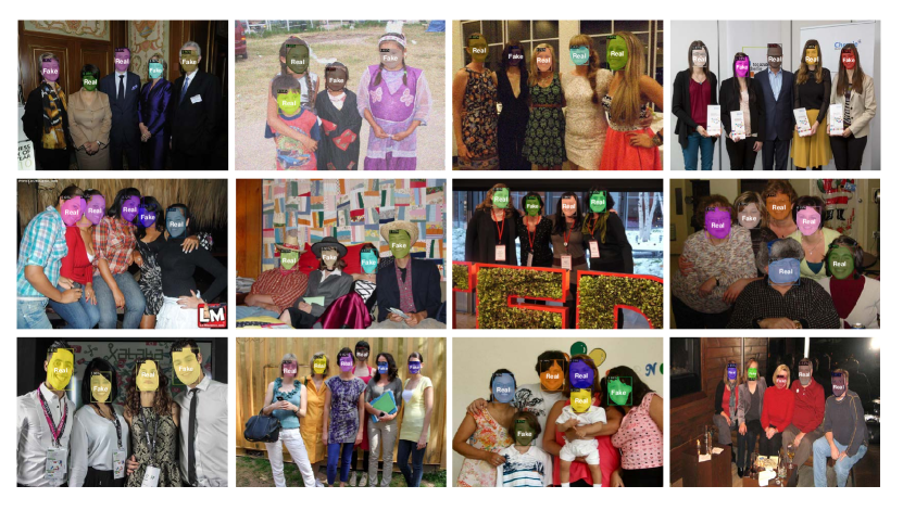
Figure 1: Our method can simultaneously detect faces and their authenticity with location and mask in an end-to-end fashion. Zoom out the faces to check the results. Best viewed in color.

Currently, the majority of DeepFake detection methods [5, 6, 7, 8] follow a two-phase pipeline that is known as face forgery recognition [9]: first, faces are extracted using face detectors; then, the faces are classified as real or DeepFake (Fig. 2 (left)). Face forgery recognition methods perform well on images or videos containing only one face in view. However, in real-world applications, an image or a video frame may have multiple faces. Applying the two-phase methods is impractical as they can only process face-by-face sequentially, resulting in longer running time or resource crunch.

Figure 2: Overview of two-phase face forgery detection (left) and the proposed single-phase face forgery detection framework Contrastive Multi-FaceForensics (right).

To expose the limitation of these two-phase methods, the OpenForenscis dataset [9] was proposed to encourage developing end-to-end pipelines, which accomplish face detection and forgery detection simultaneously. The straightforward solution is to adapt advanced object detection architectures to this task directly, and it has been shown that such adaptation is feasible to expose multi-face DeepFakes. However, since the object detectors are designed to learn the semantic features among different categories rather than the subtle characteristics that differ between real and DeepFake faces, the straightforward adaptation does not yield satisfactory results (See Sec. VII-B). Thus extra efforts are required to concentrate the network on mining face forgery traces.

In this paper, we explore a new end-to-end framework called Contrastive Multi-FaceForensics (COMICS), that solves the task of multi-face forgery detection in a single step (Fig. 2 (right)). The core component of our framework is a newly proposed Bi-grained contrastive learning scheme to expose the forgery traces among faces. Specifically, the Bi-grained contrastive learning scheme includes coarse-grained and fine-grained levels of contrastive learning. For coarse-grained contrastive learning, we first obtain the feature representations in different scales from the feature extractor corresponding to faces and design contrastive learning among positive and negative proposals, to capture the global discrepancy between real and fake faces. After that, we consider fine-grained contrastive learning to obtain local forgery traces. We first obtain the feature maps from the mask predictor corresponding to each face, and then conduct intra-face and inter-face contrastive learning at the pixel level. The intra-face learning aims to capture the pixel-wise discrepancy between forged and original areas of the same face, while inter-face learning focuses on learning the pixel-wise content inconsistency between real and fake faces. Together with the original objective of object detectors, our framework can be more effective in exposing face forgeries in an end-to-end pipeline (Fig. 3). Moreover, we propose a Frequency Enhanced Attention module, which consists of SRM filters [10] and spatial attention [11], to improve the effectiveness of features further. Extensive experiments are conducted on the OpenFaceForensics dataset compared to many state-of-the-art object adaptations, corroborating the superiority of our method in detecting multiple faces forgeries. We also conduct a comprehensive ablation study to explore the effect of different configurations and demonstrate our method can be integrated into various architectures.

Our contributions are summarized as follows:

1. We describe Contrastive Multi-FaceForensic (COMICS), an end-to-end contrastive learning framework for multi-face forgery detection in the wild. In contrast to the straight adaptation from object detection, our framework is the first to solve this task devotedly.

2. Under this end-to-end framework, we propose a new Bi-grained contrastive learning scheme that considers coarse- and fine-grained contrastive learning to capture the proposal-wise and pixel-wise forgery trace hierarchically in both inter- and intra-face manner. This learning scheme is plug-and-play, being easily adapted to different architectures.

3. Experimental results demonstrate the proposed method on the OpenForensics dataset significantly outperforms other state-of-the-art counterparts by a large margin ($\sim 18.5\%$). We also study our method regarding many factors, including the effect of each level of contrastive learning, and different parameters and settings, providing more insight for the following research.

II Related Works

Face Forgery Recognition. The conventional methods are usually two-phase based, which extract the face area first and then classify it as the real or fake category. Different types of cues are used for the classification, including physiological signals (e.g., eye blinking [12], head pose [13, 14], blood flow and heartbeats [15], domain inconsistency [16, 17, 18, 19, 20]) and signal abnormalities (e.g., face warping artifacts [21], PRNU difference [22, 23], and frequency artifacts [24, 25, 26]). Other methods designed specific architectures [27, 28, 29] and data augmentations [21, 30] to learn effective features. To further improve detection performance, many datasets are proposed, such as FaceForensics++ [31], Celeb-DF [32], DFDC [33] and etc. These datasets are constructed in a restricted environment, only containing a single subject in each video. However, the good even perfect performance on these datasets can not represent the effectiveness of existing methods, as the wild scenario usually contains multiple even dense faces, which can not be efficiently processed by two-phase methods.

Multi-face Forgery Detection. To address the above mentioned issues, OpenForensics dataset [9] was proposed to encourage the research on single-phase methods for multi-face forgery detection. In this work, several advanced object detectors are directly adapted to this task, in order to detect face area and its authenticity simultaneously [34, 35, 36, 37, 38, 39, 40]. Despite the trivial adaptation showing the feasibility of detecting multi-face forgery, they are not the optimal solution as they are not designed to capture the subtle forgery traces. Therefore, in this paper, we propose a new single-phase framework that can expose traces of DeepFake synthesis using a novel Bi-grained contrastive learning scheme.

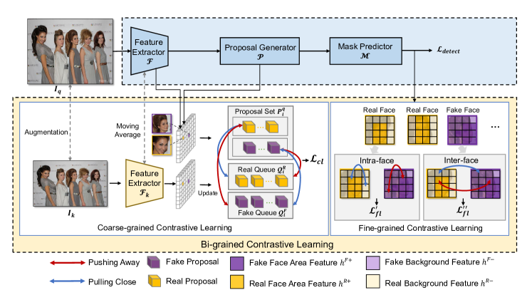
Figure 3: Overview of proposed Bi-grained contrastive learning. Our method is designed on the single-phase architecture, containing the feature extractor, the proposal generator, and the mask predictor respectively. Specifically, we perform coarse-grained contrastive learning on a feature extractor with the guidance of a proposal generator to capture the forgery traces among different face proposals, and fine-grained contrastive learning on mask predictor by considering the relationship of pixels in the same face (Intra-face) or different faces (Inter-face).

Contrastive Learning. Contrastive learning is one of the most compelling methods in both unsupervised and supervised visual representation learning domains [41, 42, 43], which has been widely used in object detection [44, 45, 46], segmentation [47, 48], medical image[49], deraining[50], person re-identification[51, 52], personalized recommendation[53, 54], image captioning [55, 56], and natural language understanding [57]. Inspired by contrastive learning, the work of [58] focused on the inconsistency between audio and visual modalities, and use a contrastive loss to model inter-modality similarity for DeepFake video detection. The work of [59] proposed a triplet network to increase the feature distance between real and fake videos in embedding feature space. CFFN [60] used the siamese network and contrastive loss to learn the discriminative features to classify GAN-generated faces. DCL [61] is the most relevant method which considered different instance-level contrastive learning. However, these methods are designed for two-phase frameworks, thus not applicable to single-phase frameworks. To fully highlight the novelty and contribution of our method, we elaborate on the difference between our method and DCL in Sec. VII-D.

III Contrastive Multi-FaceForensics

In this paper, we propose Contrastive Multi-FaceForensics (COMICS) dedicated to capturing the forgery traces among multiple faces in an end-to-end fashion. In contrast to the conventional face forgery recognition methods, our method can simultaneously expose multiple face forgeries by considering the coarse-grained and fine-grained levels of contrastive information among faces.

Network Architecture Prototype. The network architecture of our method is derived from the recent object detectors [62, 63, 64]. The object detectors are end-to-end architectures that generally contain a feature extractor, a proposal generator, and a mask predictor, respectively. They can locate the objects and give their semantic categories simultaneously. By simply restricting the object categories to two categories of real or fake faces, these architectures can be adapted to multi-face forgery detection, which thus naturally solves the limitations of face forgery recognition methods to a certain extent [9]. Inspired by that, we adopt the end-to-end architecture and propose a new Bi-grained contrastive learning scheme customized for the feature extractor, proposal generator, and mask predictor.

Bi-grained Contrastive Learning. The general contrastive learning strategy inspires our method, as the forgery traces can be further exposed by inspecting the relationship between faces. Specifically, our method seeks these relationships at the coarse-grained (proposal-wise) and fine-grained (pixel-wise) levels on the end-to-end architecture. The elements in features from the feature extractor correspond to different face proposals, and the elements in features from the mask predictor correspond to different pixels in faces. Applying Bi-grained contrastive learning can boost the network to capture the forgery traces at different levels. Using the Bi-grained contrastive learning scheme with the original end-to-end objectives can achieve the goal of effectively detecting faces and their authenticity simultaneously. Fig. 3 shows the overview of the proposed framework. Next, Sec. IV and Sec. V will introduce the detail of coarse-grained and fine-grained contrastive learning respectively.

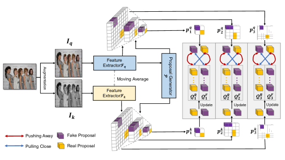
Figure 4: Overview of the coarse-grained contrastive learning. The input image is firstly augmented into two views ($I_{q},I_{k}$) and then contrastive learning is performed on proposal levels at different scales of the feature extractor. Note that the feature elements (e.g., the yellow or purple blocks) correspond to real or fake faces given the proposal generator $\mathcal{P}$.

TABLE I: Main Notations and Definitions in Proposed Method.

Notation	Definitions
$I_{q}$,$I_{k}$	input, momentum input
$\mathcal{F}_{q}$,$\mathcal{F}_{k}$	feature extractor, momentum feature extractor
${\theta}_{q}$, ${\theta}_{k}$	parameters of $\mathcal{F}_{q}$, $\mathcal{F}_{k}$
$\beta$	the exponential hyper-parameter
$f^{q}_{i}$, $f^{k}_{i}$	feature map of $I_{q}$, $I_{k}$ at the i-$th$ scale
$\mathcal{P}$	proposal generator
$P^{q}_{i}$, $P^{k}_{i}$	proposals generated from $f^{q}_{i}$, $f^{k}_{i}$
$p^{q}_{ij}$, $p^{k}_{ij}$	the j-$th$ proposal from $P^{q}_{i}$, $P^{k}_{i}$
$\mathcal{Q}^{R}_{i}$, $\mathcal{Q}^{F}_{i}$	the real/fake face queue at the i-$th$ scale
$\hat{p}_{i}^{R}$, $\hat{p}_{i}^{F}$	prototypes to update $\mathcal{Q}^{R}_{i}$, $\mathcal{Q}^{F}_{i}$
$\alpha$	hyper-parameter to update prototypes
$\delta(\cdot,\cdot)$	cosine similarity
$\omega_{i}$	weight hyper-parameters at the i-$th$ scale
$\mathcal{M}$	mask predictor
$h_{j}$	the j-$th$ predicted mask
$\mathcal{H}^{R}$, $\mathcal{H}^{F}$	predicted masks of real/fake face
$h^{R+}_{j}$, $h^{R-}_{j}$	the face area / background of $h_{j}\in\mathcal{H}^{R}$
$h^{F+}_{j}$, $h^{F-}_{j}$	the face area / background of $h_{j}\in\mathcal{H}^{F}$
$\tau$	the temperature hyper-parameter
$\lambda_{1}$, $\lambda_{2}$, $\lambda_{3}$	weight hyper-parameters for loss function
$\mathcal{L}_{detect}$	the objective loss of base detector
$\mathcal{L}_{Bi}$	the objective of Bi-grained contrastive learning
$\mathcal{L}_{cl}$	the objective of coarse-grained contrastive learning
$\mathcal{L}^{\prime}_{fl}$	the objective of intra-face fine-grained contrastive learning
$\mathcal{L}^{\prime\prime}_{fl}$	the objective of inter-face fine-grained contrastive learning

IV Coarse-grained Contrastive Learning

Coarse-grained contrastive learning focuses on capturing the discriminative forgery features among positive and negative proposals relying on feature extractor, i.e., pulling the features of proposals in the same category close and pushing away the ones of different categories. For an input image, we generate two samples of different views and design a copy of the feature extractor for contrastive learning. Then these two samples are fed into respective feature extractors to obtain proposals. By matching the proposals with faces, we conduct contrastive learning to capture the proposal-wise forgery traces. Fig. 4 shows the overview of coarse-grained contrastive learning. Following introduces the data view configuration and contrastive learning configuration respectively.

IV-A Data View Configuration.

In general classification tasks, traditional data augmentation methods (e.g., random crop, random flip, random rotation) are usually used to create different data views for contrastive learning. Since the main content is inside the image, using these augmentations can always retain the main content and enable the network to learn the content-relevant features. But in our task, the images usually contain multiple faces and our goal is to explore the relationship between these faces. Thus these general augmentations are unsuitable as they possibly disrupt the location of faces. Given the proposal generator, the position of faces between two views should be matched to easily grab corresponding faces for contrastive learning (See Fig. 4). To this end, we utilize the following augmentation methods as the second step for augmenation: 1) Color jittering and grayscale conversion. For clolor jiltteing, we randomly change the brightness, contrast, saturation and sharpness of an image with a 50% probability, respectively. For grayscale conversion, we convert the RGB images into grascale for augmentation. 2) Random blocking. We partition the image into $10\times 10$ chunks and randomly block $2\sim 6\%$ of the chunks to emphasize the forgery clues. 3) Additional noise. We employ Gaussian noise and salt-and-pepper noise. 4) Linear Interpolation. We first shrink the image into 1/4 size, then interpolate it back to its original size. These augmentation methods have a negligible effect on the position of faces but can disturb the semantic content to shed light on forgery traces. Given an image $I\in\mathbbm{R}^{H\times W\times 3}$, $I_{q}$ and $I_{k}$ are the two views using above augmentations.

IV-B Contrastive Learning Configuration.

Denote the feature extractor as $\mathcal{F}_{q}$ with parameters $\theta_{q}$. To achieve contrastive learning, we adapt the strategy in MOCO [42] to build the same feature extractor $\mathcal{F}_{k}$ with parameters ${\theta}_{k}$. The feature extractor $\mathcal{F}_{k}$ is updated as

$$\theta_{k}=\beta\cdot\theta_{k}+(1-\beta)\cdot{\theta}_{q},$$ (1)

where $\beta$ is the exponential hyper-parameter to control the update.

By feeding the image $I_{q}$ into feature extractor $\mathcal{F}_{q}$ can obtain a set of features as $\{f_{1}^{q},...,f_{n}^{q}\}=\mathcal{F}_{q}(I_{q})$. Denote the proposal generator as $\mathcal{P}$. These features are then sent into the proposal generator to create proposals on each feature as $\{P_{1}^{q},...,P_{n}^{q}\}=\mathcal{P}(\mathcal{F}_{q}(I_{q}))$, where $P_{i}^{q}$ denotes a set of proposals generated on the $i$-th feature. Similarly, for image $I_{k}$, we can obtain a set of features from copied feature extractor as $\{f^{k}_{1},...,f^{k}_{n}\}=\mathcal{F}_{k}(I_{k})$. These features are then sent into the same proposal generator $\mathcal{P}$ to create corresponding proposals as $\{P^{k}_{1},...,P^{k}_{n}\}=\mathcal{P}(\mathcal{F}_{k}(I_{k}))$.

Inter-faces. For a specific scale of $i$, we can obtain two proposal sets $P_{i}^{q}$ and $P^{k}_{i}$ corresponding to the input images $I_{q}$ and $I_{k}$. The proposal is viewed as real (fake) if IoU between this proposal and an arbitrary real (fake) face is greater than $0.6$. Then we find the corresponding feature representation of each proposal from the feature extractors. For contrastive learning, we design two queues, a real face queue $\mathcal{Q}^{R}_{i}$ and a fake face queue $\mathcal{Q}^{F}_{i}$ to store the feature representations of corresponding proposals. These queues are updated dynamically in training. Denote $p_{ij}^{q}$ and $p^{k}_{ij}$ as the feature representation of $j$-th proposal at $i$-th scale in $P^{q}_{i}$ and $P^{k}_{i}$ respectively. $\hat{p}_{i}^{R}$ and $\hat{p}_{i}^{F}$ are two prototypes used to update the real face queue $\mathcal{Q}^{R}_{i}$ and the fake face queue $\mathcal{Q}^{F}_{i}$. If $p^{k}_{ij}$ corresponds to a fake proposal, the prototype $\hat{p}_{i}^{F}$ is updated as

$$\hat{p}^{F}_{i}=\alpha\cdot\hat{p}^{F}_{i}+(1-\alpha)\cdot p^{k}_{ij},$$ (2)

where $\alpha$ is a factor controlling the update, similar to [61]. To update $\mathcal{Q}^{F}_{i}$, we calculate the similarity between $\hat{p}^{F}_{i}$ and $p^{k}_{ij}$ in a batch, and push the most dissimilar (top-5) feature of proposals into $\mathcal{Q}^{F}_{i}$. The update scheme for $\hat{p}_{i}^{R}$ and $\mathcal{Q}^{R}_{i}$ are same if $p^{k}_{ij}$ corresponds to a real proposal. The similarity between two proposals is measured using cosine similarity as

$$\delta(p^{q}_{ij},p^{k}_{ij})=\frac{p^{q}_{ij}}{\|p^{q}_{ij}\|}\cdot\frac{p^{k}_{ij}}{\|p^{k}_{ij}\|}$$ (3)

Note that on a certain scale, the number of proposals may be small. Thus we utilize FlatNCE [65] to eliminate the floating-point overflow caused by the insufficient number of samples in the training batch. The objective at $i$-th scale can be defined as

$$\mathcal{L}_{cl}^{i}=\frac{\sum_{p^{k}_{ih}\in\mathcal{Q}^{-}}e^{\delta(p^{q}_{ij},p^{k}_{ih})/\tau-\delta(p^{q}_{ij},p^{k}_{ij})/\tau}}{\texttt{Detach}(\sum_{p^{k}_{ih}\in\mathcal{Q}^{-}}e^{\delta(p^{q}_{ij},p^{k}_{ih})/\tau-\delta(p^{q}_{ij},p^{k}_{ij})/\tau})},$$ (4)

where $\texttt{Detach}(\cdot)$ is an operation that bars gradient back-propagation for the floating point relative error, and $\tau$ is the temperature parameter. $\mathcal{Q}^{-}$ denotes the negative queue corresponding to $p_{ij}$, where $\mathcal{Q}^{-}=\mathcal{Q}^{F}_{i}$ when $p_{ij}$ corresponds to a real face, otherwise $\mathcal{Q}^{-}=\mathcal{Q}^{R}_{i}$.

Multi-scale Ensemble. Since different scale contains different levels of information, we extend Equ. (4) to multi-scale contrastive losses as

$$\mathcal{L}_{cl}=\sum_{i}\omega_{i}\cdot\mathcal{L}_{cl}^{i},$$ (5)

where $\omega_{i}$ is the weight factor for different scales.

V Fine-grained Contrastive Learning

Besides the coarse-grained level, we also consider fine-grained contrastive learning, which focuses on the pixel-wise relationship in intra-face and inter-face configurations. Intra-face configuration aims to learn the inconsistency between the forged and the surrounding original area in the same face, while inter-face configuration explores the pixel-wise discrepancy between different faces. The overview of fine-grained contrastive learning is shown in Fig. 5.

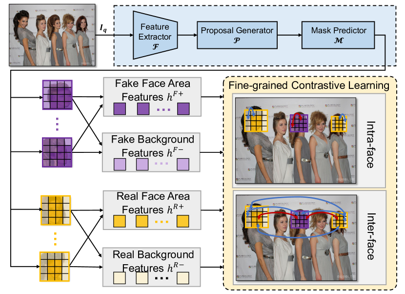
Figure 5: Overview of the fine-grained contrastive learning. In contrast to coarse-grained contrastive learning, it aims to learn the relationship among pixels instead of proposals. Given the feature maps of predicted masks, we consider two configurations of intra-face and inter-face. Specifically, intra-face configuration aims to learn the inconsistency between the forged and the surrounding original area in the same face, while inter-face configuration explores the pixel-wise discrepancy between different faces.

V-A Contrastive Learning Configuration

Denote the mask predictor as $\mathcal{M}$. Given the proposals above, we can obtain the corresponding feature maps of the predicted mask as $\{h_{1},...,h_{m}\}=\mathcal{M}(\mathcal{P}(\mathcal{F}_{q}(I_{q})))$. Here we mix the proposals of different scales into one set, where $h_{j}$ is the feature map of $j$-th predicted mask. Then we resize the feature map and the corresponding predicted mask into a fixed size for the following calculation. Denote the feature maps of predicted masks corresponding to real and fake faces as $\mathcal{H}^{R}$ and $\mathcal{H}^{F}$, respectively. Note that a mask always covers the face area and the background area. For $h_{j}\in\mathcal{H}^{R}$, both the face part and background part are original. But for $h_{j}\in\mathcal{H}^{F}$, the face part is manipulated while the background remains original. To learn the intra- and inter-face forgery traces at the pixel level, we split each predicted mask into two groups. Specifically, we denote $h^{R+}_{j}$ and $h^{R-}_{j}$ as the feature maps of the face area and the background if $h_{j}\in\mathcal{H}^{R}$, otherwise they are denoted as $h^{F+}_{j}$ and $h^{F-}_{j}$.

It is noteworthy that we do not take the pixels close to the forgery boundary into consideration, as face forgery methods usually apply postprocessing on the boundary to remove artifacts, hindering their representative forgery features compared to other pixels. In our method, we discard the pixels that have a distance within two pixels away from the boundary. The split of a mask is illustrated in Fig. 6. The following sections introduce intra-face and inter-face contrastive learning in a sequel.

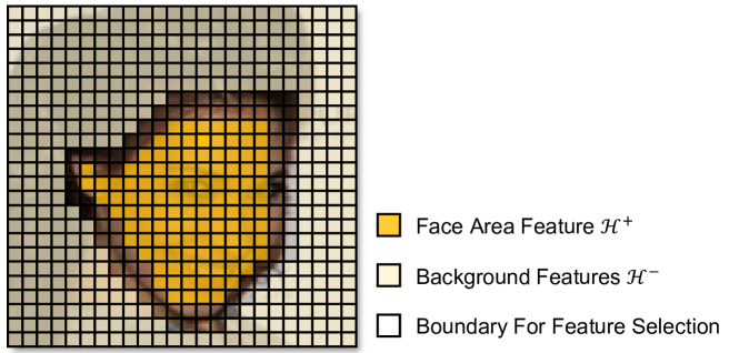
Figure 6: Illustration of mask split. In our method, we discard the pixels that have a distance within two pixels away from the boundary.

Intra-face. For a fake face, the features of the forged area should be different from the ones of the background, thus we maximize the distance between these two areas. But for a real face, these features should be similar, thus we minimize the distance between these two areas. Thus intra-face learning can be formulated as

$$\small\mathcal{L}^{\prime}_{fl}=-\log\frac{\sum\limits_{h_{j}\in\mathcal{H}^{R}}e^{\delta\left(h_{j}^{R+},h_{j}^{R-}\right)/\tau}}{\sum\limits_{h_{j}\in\mathcal{H}^{R}}e^{\delta\left((h_{j}^{R+},h_{j}^{R-}\right)/\tau}+\sum\limits_{h_{j}\in\mathcal{H}^{F}}e^{\delta\left(h_{j}^{F+},h_{j}^{F-}\right)/\tau}},$$ (6)

where $\delta(\cdot)$ is the normalized cosine similarity between two regions, as

$$\delta(h,h^{\prime})=\sum_{o\in h}\sum_{o^{\prime}\in h^{\prime}}\frac{o}{\|o\|}\cdot\frac{o^{\prime}}{\|o^{\prime}\|},$$ (7)

where $o$ denotes the feature representation of one pixel. $\tau$ is the temperature parameter.

Inter-face. Different with intra-face contrastive learning considers the content discrepancy inside a face, inter-face learning focuses on exploring the relationship between different faces. Since the backgrounds of both real and fake faces are original, we pull close the features of the backgrounds between real and fake faces. On the contrary, the face area of real and fake faces should be different, thus we push away their corresponding features. The inter-face contrastive learning can be defined as

$$\small\mathcal{L}^{\prime\prime}_{fl}=-\log\frac{\sum\limits_{h_{k}\in\mathcal{H}^{-}}e^{\delta\left(h_{j}^{R-},h_{k}^{F-}\right)/\tau}}{\sum\limits_{h_{k}\in\mathcal{H}^{-}}e^{\delta\left(h_{j}^{R-},h_{k}^{F-}\right)/\tau}+\sum\limits_{h_{k}\in\mathcal{H}^{-}}e^{\delta\left(h_{j}^{R+},h_{k}^{F+}\right)/\tau}},$$ (8)

where $\mathcal{H}^{-}$ denotes the negative set of $h_{j}$, i.e., $\mathcal{H}^{-}$ corresponds to $\mathcal{H}^{R}$ if $h_{j}$ is fake, otherwise $\mathcal{H}^{-}$ corresponds to $\mathcal{H}^{F}$.

VI Frequency Enhanced Attention and Overall Objectives

Frequency Enhanced Attention. Inspired by the previous works [66, 6, 67] that frequency domain can effectively expose forgery traces, we design a simple Frequency Enhanced Attention to enhance the importance of features indicated by high-frequency elements. Since Spatial Rich Model (SRM) filter [10] has demonstrated its effectiveness in extracting high-frequency signals, we employ it on input images and features to highlight frequency-importance features. As shown in Fig. 7, we construct a new branch that contains two convolutional layers followed by a Batch Normalization (BN) [68] and ReLu activation, and a spatial attention layer [11]. The output of this branch will be multiplied by the output of the feature extractor.

Overall Objectives. Firstly, we adapt the vanilla object detection objectives to our task, by simply modifying the semantic object categories to the category of real and fake faces. Denote the objective loss of this simple adaptation as $\mathcal{L}_{detect}$.

By considering coarse-grained and fine-grained contrastive learning, the objectives of Bi-grained contrastive learning can be written as

$$\mathcal{L}_{Bi}=\lambda_{1}\mathcal{L}_{cl}+\lambda_{2}\mathcal{L}^{\prime}_{fl}+\lambda_{3}\mathcal{L}^{\prime\prime}_{fl},$$ (9)

where $\lambda_{1}$, $\lambda_{2}$, and $\lambda_{3}$ are the hyper-parameters for the components of Bi-grained contrastive learning. Together with $\mathcal{L}_{detect}$, we can expose multi-face forgeries end-to-end (Fig. 3).

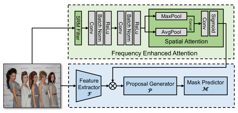
Figure 7: Illustration of frequency enhanced attention. This module aims to further improve the effectiveness of the features from feature extractors.

VII Experiments

VII-A Experimental Settings

Dataset. The experiments are performed on OpenForensics [9], which is a recently released large-scale dataset of face forgeries. OpenForensics dataset has rich annotations including class (real or fake), face forgery location and mask, which is suitable for multi-face forgery detection and segmentation. The training set contains $44,122$ images with $85,392$ real faces and $65,972$ fake faces. The validation set contains $7,308$ images including $4,786$ real faces and $10,566$ fake faces. This dataset has two testing sets according to the challenge level of detection, which is the test-development set and the test-challenge set. The images in test-development have the same distribution as the training set, while the images in test-challenge set are processed by many operations such as block-wise distortion, color manipulation, and random noise, see examples in Fig. 8. The test-development set has $18,895$ images with $21,071$ real faces and $28,670$ fake faces, while the test-challenge set has $45,000$ images with $49,218$ real faces and $68,452$ fake faces.

Evaluation Metrics. Following the same settings in [9], we use the COCO-style Average Precision (AP) and Localization Recall Precision (LRP) error for evaluation. Specifically, we evaluate the results using mean AP, AP_S, AP_M, and AP_L, where $S$, $M$, and $L$ represent small, medium, and large objects, respectively. For LRP, we present results for mean optimal LRP (oLRP), localization (oLRP_Loc), false positive rate (oLRP_FP), and false negative rate (oLRP_FN). The larger AP and less oLRP denote better performance.

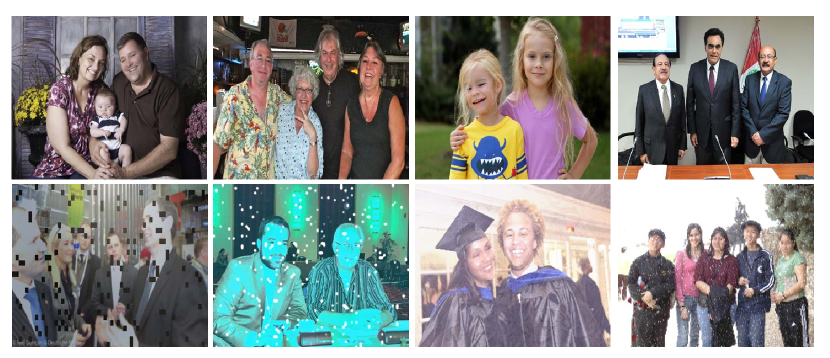
Figure 8: Image examples of OpenForensics dataset. The first row is selected from test-development set and the second row is selected from test-challenge set.

TABLE II: Comparisons of our method with others on the test-development set. Higher AP is better ($\uparrow$) and lower oLRP error is better ($\downarrow$).

Method	Multi-Face Forgery Detection								Multi-Face Forgery Segmentation
	AP	APS	APM	APL	oLRP	oLRPLoc	oLRPFP	oLRPFN	AP	APS	APM	APL	oLRP	oLRPLoc	oLRPFP	oLRPFN
MaskRCNN	79.2	29.9	80.2	79.5	24.3	9.5	2.7	4.0	83.6	16.1	82.1	85.8	21.2	7.6	3.0	4.2
MSRCNN	79.0	29.5	80.1	79.5	24.3	9.6	2.7	3.8	85.1	16.8	84.2	86.8	21.1	7.7	2.6	4.4
RetinaMask	80.0	30.9	80.2	80.7	24.2	9.0	3.0	4.6	82.8	16.4	80.6	85.1	22.6	8.1	2.9	4.9
YOLACT	68.1	12.5	67.1	69.3	37.2	13.4	6.3	8.7	72.5	3.1	67.0	75.7	34.0	11.4	6.4	8.7
YOLACT++	85.0	27.4	85.4	85.7	20.7	6.6	2.5	6.6	85.0	15.3	83.3	87.0	21.3	6.9	2.5	6.6
CenterMask	85.5	32.0	85.2	86.2	21.1	6.8	3.3	5.9	87.2	16.5	85.0	89.4	21.4	6.1	3.2	7.8
BlendMask	87.0	32.7	86.3	88.0	19.5	6.2	2.4	6.2	89.2	19.8	87.3	91.0	18.3	5.4	2.5	6.3
PolarMask	85.0	27.4	85.4	85.7	20.7	6.6	2.5	6.6	85.0	15.3	83.3	87.0	21.3	6.9	2.5	6.6
MEInst	82.8	26.0	82.7	83.4	23.8	7.6	4.1	6.8	82.2	13.9	81.5	83.3	25.0	8.1	4.0	7.2
ConInst	84.0	29.4	83.6	84.8	20.8	7.4	2.3	5.2	87.7	18.1	85.1	89.8	18.3	5.9	2.4	5.3
SOLO	-	-	-	-	-	-	-	-	86.6	15.4	85.6	88.4	20.0	6.6	2.1	6.0
SOLO2	-	-	-	-	-	-	-	-	85.1	13.7	83.7	87.1	21.5	7.1	3.1	5.8
COMICS	88.2	32.3	85.7	89.9	17.4	6.2	2.5	3.5	92.3	16.3	89.1	94.6	14.7	4.7	2.6	3.6

TABLE III: Comparisons of our method with others on the test-challenge set. Higher AP is better ($\uparrow$) and lower oLRP error is better ($\downarrow$).

Method	Multi-Face Forgery Detection								Multi-Face Forgery Segmentation
	AP	APS	APM	APL	oLRP	oLRPLoc	oLRPFP	oLRPFN	AP	APS	APM	APL	oLRP	oLRPLoc	oLRPFP	oLRPFN
MaskRCNN	42.1	11.8	46.2	40.5	65.4	13.6	29.3	40.0	43.7	4.7	44.3	44.0	64.4	11.8	29.4	41.2
MSRCNN	42.2	11.8	45.9	40.8	65.3	13.7	29.6	39.9	43.3	5.2	44.6	43.5	64.1	11.8	30.4	39.6
RetinaMask	48.5	12.8	51.0	48.1	63.3	12.6	33.2	34.6	48.0	4.7	46.5	49.7	63.3	11.8	30.9	38.0
YOLACT	49.4	5.6	49.6	50.3	60.1	15.3	23.2	29.9	51.8	1.4	47.2	54.6	58.4	13.5	23.4	30.1
YOLACT++	51.7	12.3	53.2	51.5	60.4	10.7	24.6	39.5	52.7	5.3	54.1	37.6	60.2	10.4	24.7	39.5
CenterMask	0.03	0.4	0.0	0.0	99.5	29.7	97.7	97.9	0.02	0.0	0.0	0.0	99.6	28.3	97.9	98.4
BlendMask	53.9	13.5	56.6	53.5	60.2	10.6	26.5	37.4	54.0	7.1	54.5	54.5	59.9	9.8	26.4	38.4
PolarMask	51.7	12.3	53.2	51.5	60.4	10.7	24.6	39.5	52.7	5.3	54.1	37.6	60.2	10.4	24.7	39.5
MEInst	46.1	8.6	49.9	44.9	65.9	12.4	34.6	39.7	46.0	3.8	49.0	45.2	66.2	12.6	34.8	39.8
ConInst	52.7	12.6	55.3	51.8	60.7	11.5	28.3	35.3	54.1	6.5	55.2	53.8	59.6	10.0	26.7	37.3
SOLO	-	-	-	-	-	-	-	-	55.9	3.9	53.3	57.3	57.6	11.3	24.6	33.0
SOLO2	-	-	-	-	-	-	-	-	53.2	3.6	52.1	54.0	59.6	11.0	24.5	37.2
COMICS	74.6	19.2	72.1	76.4	36.5	9.0	10.0	16.9	76.6	7.1	71.6	79.7	36.3	7.9	9.6	17.9

Implement details. All experiments were performed on a computing server equip ped with one NVIDIA GeForce RTX 3090 GPU. The base architecture is BlendMask [62], which uses FPN-ResNet50 [69] as the feature extractor. In training, the initial learning rate is set to $0.01$ and the batch size is set to $8$. We train the model for $12$ epochs on OpenForensics’ training dataset. The learning rate drops by $1/10$ at the $8$-th and $10$-th epoch. The weight hyper-parameters in Equ.(9) are set to $\lambda_{1}=0.5$, $\lambda_{2}=0.1$, and $\lambda_{3}=0.1$. For coarse-grained and fine-grained contrastive learning, we set the temperature hyper-parameter as $\tau=0.7$, the exponential hyper-parameter $\beta$ to $0.999$ and the prototypes updating parameter $\alpha$ to $0.9$. We select the $3,4,5,6,7$-th feature layers in coarse-grained learning. The weights for these layers as set to $0.1$, $0.2$, $0.4$, $0.7$ and $1.0$.

VII-B Results

Table II shows the performance of our method compared with several state-of-the-art methods on the test-development set. The compared methods are adapted from object detectors as in the original OpenForensics work [9]. The results show that our method has the best performance for mean AP and oLRP in both detection and segmentation tasks, which outperforms the runner-up (BlendMask) by $2.2\%$ at AP and $2.9\%$ at oLRP on average. Similar trends can be observed for other metrics. For a comprehensive demonstration, we plot the scatter graph of AP and oLRP. Since higher AP and lower oLRP denote better performance, the left-top corner in graph is the best. As shown in Fig. 9, our method is close to the left-top corner, notably outperforming others.

The test-challenge set contains more challenging images that are processed with different transformations. As shown in Table III, the performance of all methods significantly drops compared to the case in the test-development set. However, compared to other methods, our method has a significant improvement in all metrics. For example, our method outperforms the second best method BlendMask by $21.7\%$ at AP and $23.7\%$ at oLRP on average, which greatly corroborates that the proposed Bi-grained contrastive learning can capture more effective forgery traces than other trivial adaptations even in a challenging scenario. Similar to the above, we also plot the scatter graph of AP and oLRP in Fig. 10, showing that our method significantly outperforms others at both detection and segmentation tasks.

Compared to the performance on the test-development set, we can observe that our method significantly improves the detection results on the test-challenge set. It is because the forgery traces in the test-development set are relatively easy to be captured by all methods. However, the images in the test challenge set are subjected to various transformations, which highly suppress the forgery traces. Thus the trivial adaptations are incompetent. In contrast, our method further considers the relationship between real and fake faces by contrastive learning, thus it can capture the discriminative features more effectively.

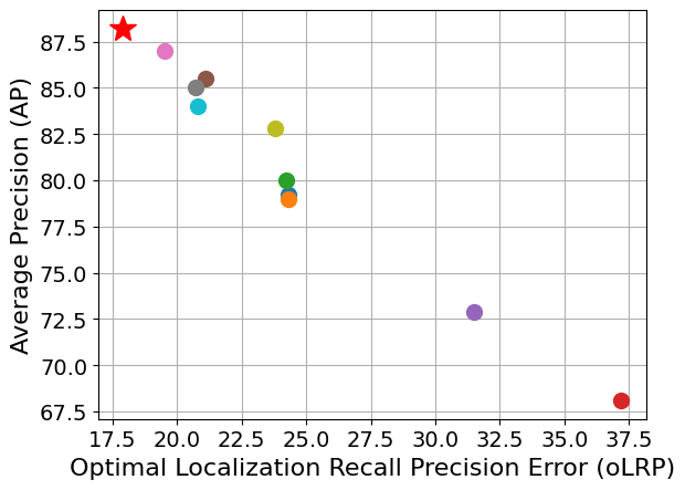
(a) Forgery Detection.

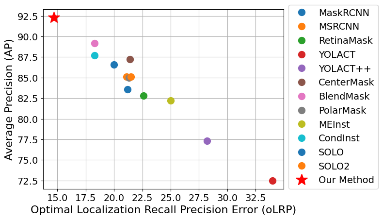
(b) Forgery Segmentation.

Figure 9: Scatter graph of AP and oLRP compared with other methods on the test-development set.

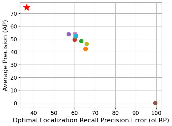
(a) Forgery Detection.

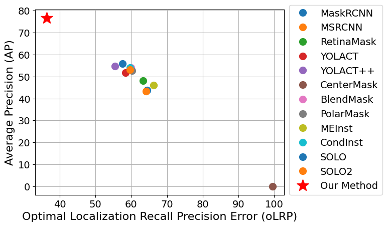
(b) Forgery Segmentation.

Figure 10: Scatter graph of AP and oLRP compared with other methods on the test-challenge set.

Fig. 11 shows several visual examples of the detection results. We use BlendMask as an example for comparison. The left group is the results of the test-development set and the right group is the ones of the test-challenge set. As shown in Fig. 11, the proposed COMICS greatly improves the face detection rate. It can be seen that BlendMask fails to identify the faces in (f)left and (d)right, and misidentifies the fake faces in (e)left and f(right), while our method successfully detects the faces as well as the forgery. Benefiting from the fine-grained learning, our method can also estimate the boundary of both real and fake faces compared to others, see the right face in (c)right and the right face in (f)left.

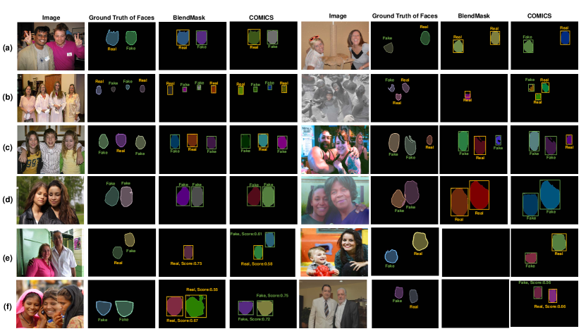
Figure 11: Visual examples of our method. We use BlendMask [62] as an example for comparison (best-performed counterpart, see Table II and Table III). The left group is the results of the test-development set and the right group is the ones of the test-challenge set.

TABLE IV: Ablation study on the effect of different components of the Contrastive Multi-FaceForensic. Higher AP is better ($\uparrow$) and lower oLRP error is better ($\downarrow$).

Test-development set Method Multi-Face Forgery Detection Multi-Face Forgery Segmentation DA FEA Bi-grained AP AP_S AP_M AP_L oLRP oLRP_Loc oLRP_FP oLRP_FN AP AP_S AP_M AP_L oLRP oLRP_Loc oLRP_FP oLRP_FN - - - 87.0 32.7 86.3 88.0 19.5 6.2 2.4 6.2 89.2 19.8 87.3 91.0 18.3 5.4 2.5 6.3 $\checkmark$ - - 88.4 30.9 85.6 90.1 17.4 6.2 2.7 3.4 91.7 14.8 88.3 94.1 15.2 4.9 2.7 3.7 - $\checkmark$ - 88.8 33.6 86.3 90.4 16.9 6.2 2.8 2.8 92.6 17.1 89.5 94.9 14.5 4.6 2.3 3.9 - - $\checkmark$ 88.9 31.7 86.0 90.5 17.4 6.1 3.1 3.3 92.3 15.0 88.9 94.5 15.2 4.7 3.0 3.9 $\checkmark$ $\checkmark$ - 88.2 31.5 85.4 90.0 17.4 6.3 2.7 3.2 92.2 16.4 88.9 94.6 14.8 4.8 2.9 3.3 - $\checkmark$ $\checkmark$ 88.3 32.9 85.6 90.0 17.7 6.3 2.9 3.5 91.6 16.3 88.3 93.8 15.6 5.0 2.9 3.8 $\checkmark$ - $\checkmark$ 88.2 31.1 85.6 89.9 17.7 6.3 2.8 3.5 91.9 14.1 88.3 94.2 15.3 4.8 2.7 3.9 $\checkmark$ $\checkmark$ $\checkmark$ 88.2 32.3 85.7 89.9 17.4 6.2 2.5 3.5 92.3 16.3 89.1 94.6 14.7 4.7 2.6 3.6 Test-Challenge Set
Method Multi-Face Forgery Detection Multi-Face Forgery Segmentation DA FEA Bi-grained AP AP_S AP_M AP_L oLRP oLRP_Loc oLRP_FP oLRP_FN AP AP_S AP_M AP_L oLRP oLRP_Loc oLRP_FP oLRP_FN - - - 53.9 13.5 56.6 53.5 60.2 10.6 26.5 37.4 54.0 7.1 54.5 54.5 59.9 9.8 26.4 38.4 $\checkmark$ - - 73.1 15.6 71.0 74.7 40.2 9.2 12.4 18.3 74.8 6.0 70.1 77.7 39.2 8.2 12.7 18.6 - $\checkmark$ - 67.5 16.4 66.0 68.9 47.0 9.6 16.5 24.6 68.1 6.3 62.7 71.5 46.4 8.5 16.5 25.7 - - $\checkmark$ 69.0 15.3 66.0 70.9 44.9 9.6 14.9 22.5 69.4 4.9 62.6 73.1 44.3 8.6 14.3 24.1 $\checkmark$ $\checkmark$ - 73.5 17.8 71.4 75.3 38.4 8.1 11.5 18.7 75.1 6.5 70.0 78.4 39.4 9.3 12.0 17.4 - $\checkmark$ $\checkmark$ 68.4 17.4 65.9 70.4 45.4 9.7 15.2 2.3 68.5 6.1 62.2 72.3 45.1 8.7 15.0 24.5 $\checkmark$ - $\checkmark$ 73.7 17.8 71.6 75.3 39.3 9.2 12.5 16.9 75.7 5.7 70.9 78.6 38.1 8.1 12.1 17.7 $\checkmark$ $\checkmark$ $\checkmark$ 74.6 19.2 72.1 76.4 36.5 9.0 10.0 16.9 76.6 7.1 71.6 79.7 36.3 7.9 9.6 17.9

VII-C Ablation Study

Effect of different components. This part studies the impact of different components of COMICS, including the proposed data augmentation, Frequency Enhanced Attention, and Bi-grained contrastive learning, respectively. The results on test-development and test-challenge sets are shown in Table IV. Note that we use BlendMask as the base architecture. DA, FEA, and Bi-grained denote specially designed data augmentations, frequency enhanced attention module, and the proposed Bi-grained contrastive learning, respectively. Without using any component, our method degrades to the base architecture (first row). Table IV shows that the proposed data augmentation brings a great improvement on the test-challenge set by $20.0\%$ at AP and $20.4\%$ on oLRP on average, suggesting the carefully designed data augmentations reveal the forged traces. Compared with base architecture, frequency enhanced attention, and Bi-grained contrastive learning separately bring an average increment of $2.6\%$ at AP and $3.2\%$ at oLRP, $2.5\%$ at AP and $2.6\%$ at oLRP on the test-development set, and $13.9\%$ at AP and $13.4\%$ on oLRP, $15.3\%$ at AP and $15.5\%$ on oLRP on the test-challenge set. Furthermore, we notice the Bi-grained contrastive learning improves the AP on small objects, indicating the SRM attention concentrates more on the forged traces. It can be seen that all the components of our method have a positive effect on the performance of the two sets. Compared with the baseline, our method improves the performance by $2.2\%$ at AP, $2.9\%$ at oLRP and $21.7\%$ at AP, $23.2\%$ at oLRP separately on average on test-development and test-challenge set.

Effect of coarse-grained Contrastive Learning and Related. This part studies the effect of different components on both the test-development set and the test-challenge set, including the effect of coarse-grained contrastive learning and the effect of using multi-scale. Table V shows the performance with and without using coarse-grained contrastive learning. Note that None denotes no Bi-grained contrastive learning is used, CL denotes coarse-grained contrastive learning is used, and CL w.o. MS denotes the multi-scale is not used in coarse-grained contrastive learning. The results reveal that coarse-grained contrastive learning improves the performance on both the test-development set and the test-challenge set by $2.1\%$ at AP, $2.8\%$ at oLRP and $21.5\%$ at AP, $23.3\%$ at oLRP respectively. To demonstrate the effect of multi-scale, we remove it from coarse-grained learning by fusing the proposals from all scales as a whole. As shown in Tab.V (Coarse w.o. MS), the performance drops by $1.7\%$ at AP, $6.2\%$ at oLRP on test-development set and $2.6\%$ at AP, $3.0\%$ at oLRP on test-challenge set, which demonstrates the effect of multi-scale.

TABLE V: Complete results of evaluation metrics in ablation study on the effect of different components.

Test-development set Method Multi-Face Forgery Detection Multi-Face Forgery Segmentation AP AP_S AP_M AP_L oLRP oLRP_Loc oLRP_FP oLRP_FN AP AP_S AP_M AP_L oLRP oLRP_Loc oLRP_FP oLRP_FN None 87.0 32.7 86.3 88.0 19.5 6.2 2.4 6.2 89.2 19.8 87.3 91.0 18.3 5.4 2.5 6.3 CL 88.1 32.8 85.4 89.8 17.5 6.3 2.9 3.1 92.3 16.4 89.1 94.5 14.7 4.7 2.7 3.6 CL w.o. MS 86.9 31.8 85.4 87.6 22.7 6.4 4.8 8.3 90.2 14.6 89.0 92.4 21.8 4.7 5.7 8.6 FL 88.1 31.9 85.7 89.7 17.6 6.3 3.1 3.6 92.1 16.8 88.9 94.4 14.9 4.7 2.7 3.9 FL w.o. inter 87.8 32.4 85.6 89.1 17.6 6.3 3.0 3.2 92.1 16.6 89.0 94.4 15.0 4.7 2.7 3.8 FL w.o. intra 88.0 31.7 85.4 89.4 17.5 6.3 2.6 3.4 92.3 16.5 89.2 94.6 14.6 4.7 2.6 3.6 COMICS (Ours) 88.2 32.3 85.7 89.9 17.4 6.2 2.5 3.5 92.3 16.3 89.1 94.6 14.7 4.7 2.6 3.6 Test-challenge set Method Multi-Face Forgery Detection Multi-Face Forgery Segmentation AP AP_S AP_M AP_L oLRP oLRP_Loc oLRP_FP oLRP_FN AP AP_S AP_M AP_L oLRP oLRP_Loc oLRP_FP oLRP_FN None 53.9 13.5 56.6 53.5 60.2 10.6 26.5 37.4 54.0 7.1 54.5 54.5 59.9 9.8 26.4 38.4 CL 74.3 18.7 72.1 76.6 37.1 9.0 9.9 16.9 76.5 6.9 71.5 79.0 36.4 7.9 9.9 17.9 CL w.o. MS 71.8 18.4 72.2 73.6 39.7 9.0 11.5 18.7 73.8 7.1 71.5 79.8 39.8 7.9 11.4 19.3 FL 73.5 18.7 72.2 76.3 38.4 9.0 10.6 17.2 75.9 7.2 71.5 79.1 36.5 8.0 10.0 18.0 FL w.o. inter 73.6 18.7 71.8 76.5 39.6 9.0 10.4 17.7 75.6 7.0 71.5 78.7 37.4 8.0 9.9 18.6 FL w.o. intra 73.3 19.2 72.0 76.1 38.9 9.1 9.8 17.4 75.5 6.9 71.1 78.6 37.5 8.1 9.9 18.8 COMICS (Ours) 74.6 19.2 72.1 76.4 36.5 9.0 10.0 16.9 76.6 7.1 71.6 79.7 36.3 7.9 9.6 17.9

Effect of Fine-grained Contrastive Learning and Related. This part studies the effect of using fine-grained contrastive learning (FL), only using intra-face loss (FL w.o. inter) and only using inter-face loss (FL w.o. intra). The results are also shown in Table V. By adding the fine-grained contrastive leaning, the performance is improved by $2.0\%$ at AP and $2.7\%$ at oLRP on the test-development set, and $20.8\%$ at AP, $22.6\%$ at oLRP on the test-challenge set. Moreover, the intra-face loss (FL w.o. inter) improves the performance on test sets by $11.3\%$ at AP and $12.1\%$ at oLRP on average. The inter-face loss (FL w.o. intra) brings $11.3\%$ and $12.4\%$ performance improvement at AP and oLRP on average, which demonstrates the effectiveness of conducting fine-grained contrastive learning in both inter- and intra-face aspects.

Sample Selection in Fine-grained Contrastive Learning. This part studies the effect of different sample selections in fine-grained contrastive learning. Specifically, we explore two more cases, selecting samples close to the forgery boundary (Close), and selecting all samples (All). Note that selecting samples far from the forgery boundary is used in our method. Table VI shows the performance of using different sample selections. It can be seen that using samples far from the forgery boundary achieves the best performance, which is because the forgery boundary is usually smoothed by image processing methods, disrupting the feature representation of nearby samples.

TABLE VI: Complete results of evaluation metrics in ablation study on sample selection strategies.

Test-development set Method Multi-Face Forgery Detection Multi-Face Forgery Segmentation AP AP_S AP_M AP_L oLRP oLRP_Loc oLRP_FP oLRP_FN AP AP_S AP_M AP_L oLRP oLRP_Loc oLRP_FP oLRP_FN All 87.1 30.8 85.5 89.7 17.7 6.5 3.0 3.5 92.1 16.7 89.0 94.4 15.0 4.7 2.9 3.6 Close 87.1 31.8 85.4 89.6 17.6 6.3 2.6 3.5 92.3 16.1 89.1 94.5 14.7 4.6 2.5 3.9 COMICS (Ours) 88.2 32.3 85.7 89.9 17.4 6.2 2.5 3.5 92.3 16.3 89.1 94.6 14.7 4.7 2.6 3.6 Test-challenge set Method Multi-Face Forgery Detection Multi-Face Forgery Segmentation AP AP_S AP_M AP_L oLRP oLRP_Loc oLRP_FP oLRP_FN AP AP_S AP_M AP_L oLRP oLRP_Loc oLRP_FP oLRP_FN All 74.6 18.9 71.9 76.4 37.5 9.0 9.7 17.2 76.5 6.9 71.3 79.6 36.2 7.8 9.2 18.1 Close 73.9 18.8 71.9 75.6 37.7 9.0 10.3 17.2 76.4 6.9 71.4 79.5 36.0 7.9 9.6 17.5 COMICS (Ours) 74.6 19.2 72.1 76.4 36.5 9.0 10.0 16.9 76.6 7.1 71.6 79.7 36.3 7.9 9.6 17.9

Effect of different Weights in Loss. Table VII shows the performance of different weights in the loss of Bi-grained contrastive learning on the test-development set (top) and test-challenge set (bottom), respectively. Specifically, $\lambda_{1}$ is selected from $\{1,0.5\}$, $\lambda_{2}$ is selected from $\{1,0.5,0.1\}$, $\lambda_{3}$ is selected from $\{1,0.1\}$. The results show that different weights achieve similar performance, which demonstrates the robustness of our method against different weights. We use $\lambda_{1}=0.5$, $\lambda_{2}=0.1$, and $\lambda_{3}=0.1$ in our method.

TABLE VII: Ablation study on weights of Bi-grained contrastive learning.

Test-development set $\lambda_{1},\lambda_{2},\lambda_{3}$ Multi-Face Forgery Detection Multi-Face Forgery Segmentation AP AP_S AP_M AP_L oLRP oLRP_Loc oLRP_FP oLRP_FN AP AP_S AP_M AP_L oLRP oLRP_Loc oLRP_FP oLRP_FN 1.0,1.0,0.1 88.1 32.3 85.4 89.7 17.7 6.3 2.7 3.6 92.1 16.5 88.8 94.4 15.0 4.7 2.8 3.7 1.0,0.5,0.1 88.2 32.2 85.6 90.0 17.5 6.2 2.8 3.4 92.2 16.2 88.9 94.5 14.8 4.7 2.8 3.6 1,0.1,0.1.0 88.3 32.4 85.7 90.0 17.4 6.2 2.4 3.8 92.3 16.7 89.0 94.5 14.7 4.6 2.4 3.9 0.5,0.5,1.0 88.2 32.2 85.5 89.9 17.5 6.3 2.7 3.5 92.2 16.3 89.0 94.5 14.8 4.6 2.6 3.8 0.5,0.1,0.1 88.2 32.3 85.7 89.9 17.4 6.2 2.5 3.5 92.3 16.3 89.1 94.6 14.7 4.7 2.6 3.6 Test-challenge set $\lambda_{1},\lambda_{2},\lambda_{3}$ Multi-Face Forgery Detection Multi-Face Forgery Segmentation AP AP_S AP_M AP_L oLRP oLRP_Loc oLRP_FP oLRP_FN AP AP_S AP_M AP_L oLRP oLRP_Loc oLRP_FP oLRP_FN 1.0,1.0,0.1 74.8 19.2 72.2 76.6 37.1 9.0 8.9 17.3 76.7 7.1 71.4 80.0 35.8 7.8 9.1 17.7 1.0,0.5,0.1 74.9 19.4 72.2 76.8 37.2 9.1 9.9 16.4 76.8 7.2 71.5 80.0 36.0 7.9 9.6 17.2 1.0,0.1,0.1 74.7 19.1 72.1 76.7 37.6 9.1 10.4 16.3 76.7 7.0 71.5 79.9 36.3 7.9 10.1 17.2 0.5,0.5,1.0 74.7 18.8 71.9 76.6 37.3 9.1 9.7 16.6 76.8 7.0 71.5 80.0 36.0 7.9 9.3 17.5 0.5,0.1,0.1 74.6 19.2 72.1 76.4 36.5 9.0 10.0 16.9 76.6 7.1 71.6 79.7 36.3 7.9 9.6 17.9

Effect of different Temperatures in Bi-grained contrastive learning. Temperature plays an important role in Bi-grained contrastive learning as it controls the strength of penalties on hard examples. In this part, we study the effect of different temperature hyper-parameters in Bi-grained contrastive learning on the test-development set and the test-challenge set in Tab. VIII. Specifically, we set $\tau$ to $0.07,0.2,0.7$ respectively. Note that small temperatures enable the models to focus more on the hard examples, which is consistent with the results in Tab.VIII, that small $\tau$ improves the performance slightly on the test-challenge set but declines slightly on the test-development set. We take $\tau=0.7$ in our method for better balance.

TABLE VIII: Ablation study on temperature hyper-parameter.

Test-development set Temperature $\tau$ Multi-Face Forgery Detection Multi-Face Forgery Segmentation AP AP_S AP_M AP_L oLRP oLRP_Loc oLRP_FP oLRP_FN AP AP_S AP_M AP_L oLRP oLRP_Loc oLRP_FP oLRP_FN $\tau=0.07$ 87.8 31.1 85.3 89.5 17.9 6.4 3.0 3.3 92.1 16.2 88.8 94.2 15.1 4.7 2.7 3.9 $\tau=0.2$ 87.9 32.2 85.3 89.6 17.9 6.4 3.2 3.1 92.2 16.4 88.9 94.3 15.1 4.7 2.8 3.8 $\tau=0.7$ 88.2 32.3 85.7 89.9 17.4 6.2 2.5 3.5 92.3 16.3 89.1 94.6 14.7 4.7 2.6 3.6 Test-challenge set Temperature $\tau$ Multi-Face Forgery Detection Multi-Face Forgery Segmentation AP AP_S AP_M AP_L oLRP oLRP_Loc oLRP_FP oLRP_FN AP AP_S AP_M AP_L oLRP oLRP_Loc oLRP_FP oLRP_FN $\tau=0.07$ 74.1 18.4 71.8 76.1 37.7 9.1 9.7 17.4 76.5 7.1 71.5 79.5 36.3 7.9 9.5 17.9 $\tau=0.2$ 75.2 19.4 72.4 77.1 36.6 9.1 9.4 15.8 77.3 7.2 71.9 80.4 35.3 8.0 9.4 16.3 $\tau=0.7$ 74.6 19.2 72.1 76.4 36.5 9.0 10.0 16.9 76.6 7.1 71.6 79.7 36.3 7.9 9.6 17.9

Integrating our framework to different architectures. To demonstrate the effectiveness of the proposed Bi-grained contrastive learning, we integrate it into other different detection architectures: MaskRCNN [70], ConInst [64], MEInst [38] and SOLOv2 [37]. The results in Tab. IX show that the proposed framework improves the detection and segmentation performance on all the benchmarks. MaskRCNN is a well-known two-stage models that perform detect-then-segment, and the performance is improved by the proposed framework by $15.2\%$ and $11.1\%$ at AP and oLRP on average. ConInst and MEInst are two one-stage detection models. The performance of ConInst after integration is improved by $11.6\%$ at AP, $11.3\%$ at oLRP on average. The improvement for MEInst is $13.1\%$ and $12.6\%$ at AP and oLRP on average. For SOLOv2, the segmentation performance is improved by $8.7\%$ at AP and $8.2\%$ at oLRP on average. This experiment can demonstrate that the proposed Contrastive Multi-FaceForensics framework can be integrated into various architectures.

TABLE IX: Complete results of evaluation metrics in ablation study on integrating our framework into different architectures.

Test-development set Method Multi-Face Forgery Detection Multi-Face Forgery Segmentation AP AP_S AP_M AP_L oLRP oLRP_Loc oLRP_FP oLRP_FN AP AP_S AP_M AP_L oLRP oLRP_Loc oLRP_FP oLRP_FN MaskRCNN 79.2 29.9 80.2 79.5 24.3 9.5 2.7 4.0 83.6 16.1 82.1 85.8 21.2 7.6 3.0 4.2 MaskRCNN-COMICS 85.5 26.3 83.8 86.8 21.1 7.3 3.8 4.4 89.6 13.1 86.9 91.8 19.0 5.9 3.4 5.3 ConInst 84.0 29.4 83.6 84.8 20.8 7.4 2.3 5.2 87.7 18.1 85.1 89.8 18.3 5.9 2.4 5.3 ConInst-COMICS 87.4 29.9 85.0 89.0 18.2 6.5 3.3 3.1 91.0 14.8 87.1 93.4 16.0 5.2 2.8 4.0 MEInst 82.8 26.0 82.7 83.4 23.8 7.6 4.1 6.8 82.2 13.9 81.5 83.3 25.0 8.1 4.0 7.2 MEInst-COMICS 86.8 26.3 83.6 88.7 21.0 7.1 3.6 6.0 87.5 12.8 83.5 89.9 21.0 7.9 3.7 4.2 SOLOv2 - - - - - - - - 85.1 13.7 83.7 87.1 21.5 7.1 3.1 5.8 SOLOv2-COMICS - - - - - - - - 85.5 7.7 82.1 88.4 21.5 7.3 3.6 5.1 Test-challenge set Method Multi-Face Forgery Detection Multi-Face Forgery Segmentation AP AP_S AP_M AP_L oLRP oLRP_Loc oLRP_FP oLRP_FN AP AP_S AP_M AP_L oLRP oLRP_Loc oLRP_FP oLRP_FN MaskRCNN 42.1 11.8 46.2 40.5 65.4 13.6 29.3 40.0 43.7 4.7 44.3 44.0 64.4 11.8 29.4 41.2 MaskRCNN-COMICS 65.8 14.2 65.1 66.5 46.1 10.2 15.5 22.7 68.3 5.3 65.3 70.2 44.8 8.8 15.4 23.3 ConInst 52.7 12.6 55.3 51.8 60.7 11.5 28.3 35.3 54.1 6.5 55.2 53.8 59.6 10.0 26.7 37.3 ConInst-COMICS 72.1 17.4 70.6 73.5 40.7 9.0 11.7 20.3 74.4 6.5 70.5 76.9 39.5 8.0 11.8 20.4 MEInst 46.1 8.6 49.9 44.9 65.9 12.4 34.6 39.7 46.0 3.8 49.0 45.2 66.2 12.6 34.8 39.8 MEInst-COMICS 67.2 15.8 63.8 69.0 44.3 11.7 12.3 19.1 68.0 1.9 63.6 70.8 44.2 11.4 12.2 19.5 SOLOv2 - - - - - - - - 53.2 3.6 52.1 54.0 59.6 11.0 24.5 37.2 SOLOv2-COMICS - - - - - - - - 70.2 2.9 65.3 73.0 43.2 11.0 11.9 19.2

VII-D Discussions

Highlight the Novelty and Contribution. As described in Sec. II, DCL [61] is the most relevant method to us, which is a recent two-phase face forgery detection method that also utilizes contrastive learning on different levels. Thus we take DCL as the most representative counterpart and elaborately highlight our method’s novelty and contributions as follows.

1) Differences on task. DCL belongs to the face forgery recognition task that extracts the face and then performs classification. In contrast, our method focuses on multi-face forgery detection, simultaneously accomplishing multiple face forgery detection in an end-to-end fashion. Fundamentally, DCL targets a classification task, while ours targets a detection task, which naturally leads to a significant difference between the pipeline of these two works. Therefore, it is difficult and unlikely to adapt the strategy proposed in DCL to our framework directly.

2) Differences in architecture and corresponding principle. DCL utilizes typical classification networks. Since only one face is contained in the view, the whole feature map of the network can represent the face. However, Contrastive Multi-FaceForensics is based on the anchor-free based detection architecture (e.g., BlendMask), which contains a backbone network, a proposal generator, and a mask predictor, respectively. Since many faces are in the view, the features have entirely different meanings compared to DCL, which does not correspond to a single face but is a mixture of all faces. It is easy for DCL to perform contrastive learning on features. At the same time, the case is different for our work, as we need to look closer into the architecture and disentangle the features of interest using a proposal generator and mask predictor to seek the relationship of different faces.

3) The novelty of proposed Bi-grained contrastive learning. Both of us and DCL borrow the concept of contrastive learning from the work of MOCO [42]. The formulation is similar since we all intend to find the relationships between specific units. But the difference is how to select and formulate the units, e.g., the queues and corresponding spirits have different meanings. In contrast to the plain contrastive learning in DCL, our method contains coarse-grained contrastive learning that is performed proposal-wise with the guide of a proposal generator and fine-grained contrastive learning that is performed in a manner of inter-face and intra-face pixel-wise, with the guide of mask predictor. Despite DCL also considering inter-face and intra-face, they are entirely different from us, as the inter-face in DCL measures the relationship of faces in different images, not proposals in the same image, and the intra-face only measures the relationships of pixels inside a face, without considering different faces. Thus they cannot handle the problem of multi-face forgery detection and hardly be applied to single-phase architecture.

Dataset Selection. Note that the number of datasets for multi-face forgery detection is significantly less than it is for conventional face forgery recognition. To the best of our knowledge, the recent OpenForensics dataset [9] and FFIW dataset [71] contain multiple faces in a view. However, the FFIW dataset only contains the ground truth of fake faces while the location of real faces is unknown, thus it is not applicable to our task. In comparison, the OpenForensics dataset has full annotations for real and fake faces, which can be friendly used in training and testing for our method.

Limitations. Contrastive Multi-FaceForensic is designed on recent detection architecture (anchor-based or anchor-free). Thus, it may inherit the drawbacks of such architecture, such as not being sensitive to small faces. This limitation is demonstrated by the results in Table II, where our method drops slightly in detecting small faces.

VIII Conclusion

In this paper, we describe a new framework called Contrastive Multi-FaceForensics (COMICS) for multi-face forgery detection. Different from the recent face forgery recognition methods, our method can simultaneously expose multiple real and fake faces in a view, using the newly proposed Bi-grained contrastive learning. Compared to the existing trivial adaptions from object detectors, the Bi-grained contrastive learning scheme is devoted to capturing the forgery traces in single-phase architecture from the perspectives of coarse-grained and fine-grained. The coarse-grained learning is performed on feature extractors, which focuses on the proposal-wise discrepancy in a multi-scale manner, guided by the proposal generator. The fine-grained learning focuses on the feature maps obtained by mask predictor and targets the pixel-wise discrepancy in both inter-face and intra-face configurations. Extensive experiments are conducted on the OpenForensics dataset with the comparison to several recent counterparts, showing that our method significantly outperforms other methods in challenging scenarios. We also conduct comprehensive ablation studies to investigate the effect of different settings involved in the configuration of Bi-grained contrastive learning.

References

- [1] L. Li, J. Bao, H. Yang, D. Chen, and F. Wen, “Faceshifter: Towards high fidelity and occlusion aware face swapping,” arXiv preprint arXiv:1912.13457, 2019.
- [2] S. Xiao, G. Lan, J. Yang, W. Lu, Q. Meng, and X. Gao, “Mcs-gan: A different understanding for generalization of deep forgery detection,” IEEE Transactions on Multimedia, pp. 1–13, 2023.
- [3] Y. Wu, W. AbdAlmageed, and P. Natarajan, “Mantra-net: Manipulation tracing network for detection and localization of image forgeries with anomalous features,” in IEEE Computer Vision and Pattern Recognition Conference (CVPR), 2019, pp. 9543–9552.
- [4] Z. Yang, J. Liang, Y. Xu, X.-Y. Zhang, and R. He, “Masked relation learning for deepfake detection,” IEEE Transactions on Information Forensics and Security (TIFS), vol. 18, pp. 1696–1708, 2023.
- [5] H. Zhao, W. Zhou, D. Chen, T. Wei, W. Zhang, and N. Yu, “Multi-attentional deepfake detection,” in IEEE Computer Vision and Pattern Recognition Conference (CVPR), 2021, pp. 2185–2194.
- [6] X. Chen, C. Dong, J. Ji, J. Cao, and X. Li, “Image manipulation detection by multi-view multi-scale supervision,” in IEEE Computer Vision and Pattern Recognition Conference (CVPR), 2021, pp. 14 185–14 193.
- [7] Z. Gu, T. Yao, C. Yang, R. Yi, S. Ding, and L. Ma, “Region-aware temporal inconsistency learning for deepfake video detection,” in Proceedings of the Thirty-First International Joint Conference on Artificial Intelligence (IJCAI), vol. 1, 2022.
- [8] R. Han, X. Wang, N. Bai, Q. Wang, Z. Liu, and J. Xue, “Fcd-net: Learning to detect multiple types of homologous deepfake face images,” IEEE Transactions on Information Forensics and Security (TIFS), 2023.
- [9] T.-N. Le, H. H. Nguyen, J. Yamagishi, and I. Echizen, “Openforensics: Large-scale challenging dataset for multi-face forgery detection and segmentation in-the-wild,” in IEEE Computer Vision and Pattern Recognition Conference (CVPR), 2021, pp. 10 117–10 127.
- [10] J. Fridrich and J. Kodovsky, “Rich models for steganalysis of digital images,” IEEE Transactions on information Forensics and Security (TIFS), vol. 7, no. 3, pp. 868–882, 2012.
- [11] S. Woo, J. Park, J.-Y. Lee, and I. S. Kweon, “Cbam: Convolutional block attention module,” in Proceedings of the European conference on computer vision (European Conference on Computer Vision (ECCV)), 2018, pp. 3–19.
- [12] Y. Li, M.-C. Chang, and S. Lyu, “In ictu oculi: Exposing ai created fake videos by detecting eye blinking,” in IEEE international workshop on information forensics and security (WIFS). IEEE, 2018, pp. 1–7.
- [13] X. Yang, Y. Li, H. Qi, and S. Lyu, “Exposing gan-synthesized faces using landmark locations,” in Proceedings of the ACM workshop on information hiding and multimedia security, 2019, pp. 113–118.
- [14] N. S. Ivanov, A. V. Arzhskov, and V. G. Ivanenko, “Combining deep learning and super-resolution algorithms for deep fake detection,” in 2020 IEEE Conference of Russian Young Researchers in Electrical and Electronic Engineering (EIConRus). IEEE, 2020, pp. 326–328.
- [15] U. A. Ciftci, I. Demir, and L. Yin, “Fakecatcher: Detection of synthetic portrait videos using biological signals,” IEEE transactions on pattern analysis and machine intelligence (TPAMI), 2020.
- [16] A. Haliassos, R. Mira, S. Petridis, and M. Pantic, “Leveraging real talking faces via self-supervision for robust forgery detection,” in IEEE Computer Vision and Pattern Recognition Conference (CVPR), 2022, pp. 14 950–14 962.
- [17] W. Yang, X. Zhou, Z. Chen, B. Guo, Z. Ba, Z. Xia, X. Cao, and K. Ren, “Avoid-df: Audio-visual joint learning for detecting deepfake,” IEEE Transactions on Information Forensics and Security (TIFS), vol. 18, pp. 2015–2029, 2023.
- [18] C. Zhao, C. Wang, G. Hu, H. Chen, C. Liu, and J. Tang, “Istvt: interpretable spatial-temporal video transformer for deepfake detection,” IEEE Transactions on Information Forensics and Security (TIFS), vol. 18, pp. 1335–1348, 2023.
- [19] Z. Guo, G. Yang, J. Chen, and X. Sun, “Exposing deepfake face forgeries with guided residuals,” IEEE Transactions on Multimedia(TMM), pp. 1–14, 2023.
- [20] Y. Yu, X. Zhao, R. Ni, S. Yang, Y. Zhao, and A. C. Kot, “Augmented multi-scale spatiotemporal inconsistency magnifier for generalized deepfake detection,” IEEE Transactions on Multimedia(TMM), pp. 1–13, 2023.
- [21] Y. Li and S. Lyu, “Exposing deepfake videos by detecting face warping artifacts,” arXiv preprint arXiv:1811.00656, 2018.
- [22] M. Koopman, A. M. Rodriguez, and Z. Geradts, “Detection of deepfake video manipulation,” in The 20th Irish machine vision and image processing conference (IMVIP), 2018, pp. 133–136.
- [23] L. Zhang, T. Qiao, M. Xu, N. Zheng, and S. Xie, “Unsupervised learning-based framework for deepfake video detection,” IEEE Transactions on Multimedia(TMM), pp. 1–15, 2022.
- [24] J. Frank, T. Eisenhofer, L. Schönherr, A. Fischer, D. Kolossa, and T. Holz, “Leveraging frequency analysis for deep fake image recognition,” in International Conference on Machine Learning (ICML). PMLR, 2020, pp. 3247–3258.
- [25] R. Durall, M. Keuper, F.-J. Pfreundt, and J. Keuper, “Unmasking deepfakes with simple features,” arXiv preprint arXiv:1911.00686, 2019.
- [26] L. Song, Z. Fang, X. Li, X. Dong, Z. Jin, Y. Chen, and S. Lyu, “Adaptive face forgery detection in cross domain,” in European Conference on Computer Vision (ECCV). Springer, 2022, pp. 467–484.
- [27] D. Afchar, V. Nozick, J. Yamagishi, and I. Echizen, “Mesonet: a compact facial video forgery detection network,” in IEEE international workshop on information forensics and security (WIFS). IEEE, 2018, pp. 1–7.
- [28] Z. Liu, X. Qi, and P. H. Torr, “Global texture enhancement for fake face detection in the wild,” in IEEE Computer Vision and Pattern Recognition Conference (CVPR), 2020, pp. 8060–8069.
- [29] Y. Luo, Y. Zhang, J. Yan, and W. Liu, “Generalizing face forgery detection with high-frequency features,” in IEEE Computer Vision and Pattern Recognition Conference (CVPR), 2021, pp. 16 317–16 326.
- [30] K. Shiohara and T. Yamasaki, “Detecting deepfakes with self-blended images,” in IEEE Computer Vision and Pattern Recognition Conference (CVPR), 2022, pp. 18 720–18 729.
- [31] A. Rossler, D. Cozzolino, L. Verdoliva, C. Riess, J. Thies, and M. Nießner, “Faceforensics++: Learning to detect manipulated facial images,” in IEEE Computer Vision and Pattern Recognition Conference (CVPR), 2019, pp. 1–11.
- [32] Y. Li, X. Yang, P. Sun, H. Qi, and S. Lyu, “Celeb-df: A large-scale challenging dataset for deepfake forensics,” in IEEE Computer Vision and Pattern Recognition Conference (CVPR), 2020, pp. 3207–3216.
- [33] B. Dolhansky, R. Howes, B. Pflaum, N. Baram, and C. C. Ferrer, “The deepfake detection challenge (dfdc) preview dataset,” arXiv preprint arXiv:1910.08854, 2019.
- [34] E. Xie, P. Sun, X. Song, W. Wang, X. Liu, D. Liang, C. Shen, and P. Luo, “Polarmask: Single shot instance segmentation with polar representation,” in IEEE Computer Vision and Pattern Recognition Conference (CVPR), 2020, pp. 12 193–12 202.
- [35] D. Bolya, C. Zhou, F. Xiao, and Y. J. Lee, “Yolact++: Better real-time instance segmentation,” IEEE transactions on pattern analysis and machine intelligence (TPAMI), 2020.
- [36] ——, “Yolact: Real-time instance segmentation,” in Proceedings of the IEEE/CVF international conference on computer vision (ICCV), 2019, pp. 9157–9166.
- [37] X. Wang, R. Zhang, T. Kong, L. Li, and C. Shen, “Solov2: Dynamic and fast instance segmentation,” Advances in neural information processing systems (NeurIPS), vol. 33, pp. 17 721–17 732, 2020.
- [38] R. Zhang, Z. Tian, C. Shen, M. You, and Y. Yan, “Mask encoding for single shot instance segmentation,” in IEEE Computer Vision and Pattern Recognition Conference (CVPR), 2020, pp. 10 226–10 235.
- [39] Y. Lee and J. Park, “Centermask: Real-time anchor-free instance segmentation,” in IEEE Computer Vision and Pattern Recognition Conference (CVPR), 2020, pp. 13 906–13 915.
- [40] Z. Cai, Q. Fan, R. S. Feris, and N. Vasconcelos, “A unified multi-scale deep convolutional neural network for fast object detection,” in European Conference on Computer Vision (ECCV). Springer, 2016, pp. 354–370.
- [41] T. Chen, S. Kornblith, M. Norouzi, and G. Hinton, “A simple framework for contrastive learning of visual representations,” in International Conference on Machine Learning (ICML). PMLR, 2020, pp. 1597–1607.
- [42] K. He, H. Fan, Y. Wu, S. Xie, and R. Girshick, “Momentum contrast for unsupervised visual representation learning,” in IEEE Computer Vision and Pattern Recognition Conference (CVPR), 2020, pp. 9729–9738.
- [43] Y. Zhang, Y. Liu, Y. Xu, H. Xiong, C. Lei, W. He, L. Cui, and C. Miao, “Enhancing sequential recommendation with graph contrastive learning,” in Proceedings of the Thirty-First International Joint Conference on Artificial Intelligence (IJCAI), 2022.
- [44] E. Xie, J. Ding, W. Wang, X. Zhan, H. Xu, P. Sun, Z. Li, and P. Luo, “Detco: Unsupervised contrastive learning for object detection,” in IEEE Computer Vision and Pattern Recognition Conference (CVPR), 2021, pp. 8392–8401.
- [45] Y. Li, Q. Wang, X. Luo, and J. Yin, “Class-balanced contrastive learning for fine-grained airplane detection,” IEEE Geoscience and Remote Sensing Letters, vol. 19, pp. 1–5, 2022.
- [46] M. Zhang, Q. Li, Y. Yuan, and Q. Wang, “Edge neighborhood contrastive learning for building change detection,” IEEE Geoscience and Remote Sensing Letters, 2022.
- [47] X. Wang, K. Zhao, R. Zhang, S. Ding, Y. Wang, and W. Shen, “Contrastmask: Contrastive learning to segment every thing,” in IEEE Computer Vision and Pattern Recognition Conference (CVPR), 2022, pp. 11 604–11 613.
- [48] T. Wang, J. Lu, Z. Lai, J. Wen, and H. Kong, “Uncertainty-guided pixel contrastive learning for semi-supervised medical image segmentation,” in Proceedings of the Thirty-First International Joint Conference on Artificial Intelligence (IJCAI), 2022, pp. 1444–1450.
- [49] Z. Liu, Z. Zhu, S. Zheng, Y. Liu, J. Zhou, and Y. Zhao, “Margin preserving self-paced contrastive learning towards domain adaptation for medical image segmentation,” IEEE Journal of Biomedical and Health Informatics, vol. 26, no. 2, pp. 638–647, 2022.
- [50] X. Chen, J. Pan, K. Jiang, Y. Li, Y. Huang, C. Kong, L. Dai, and Z. Fan, “Unpaired deep image deraining using dual contrastive learning,” in IEEE Computer Vision and Pattern Recognition Conference (CVPR), 2022, pp. 2017–2026.
- [51] X. Song and Z. Jin, “Robust label rectifying with consistent contrastive-learning for domain adaptive person re-identification,” IEEE Transactions on Multimedia, vol. 24, pp. 3229–3239, 2022.
- [52] T. Si, F. He, Z. Zhang, and Y. Duan, “Hybrid contrastive learning for unsupervised person re-identification,” IEEE Transactions on Multimedia, pp. 1–1, 2022.
- [53] K. Liu, F. Xue, D. Guo, P. Sun, S. Qian, and R. Hong, “Multimodal graph contrastive learning for multimedia-based recommendation,” IEEE Transactions on Multimedia, pp. 1–13, 2023.
- [54] D. Cai, S. Qian, Q. Fang, J. Hu, W. Ding, and C. Xu, “Heterogeneous graph contrastive learning network for personalized micro-video recommendation,” IEEE Transactions on Multimedia, vol. 25, pp. 2761–2773, 2023.
- [55] B. Dai and D. Lin, “Contrastive learning for image captioning,” Advances in neural information processing systems (NeurIPS), vol. 30, 2017.
- [56] Z. Li, Q. Tran, L. Mai, Z. Lin, and A. L. Yuille, “Context-aware group captioning via self-attention and contrastive features,” in IEEE Computer Vision and Pattern Recognition Conference (CVPR), 2020, pp. 3440–3450.
- [57] Y. Qu, D. Shen, Y. Shen, S. Sajeev, J. Han, and W. Chen, “Coda: Contrast-enhanced and diversity-promoting data augmentation for natural language understanding,” arXiv preprint arXiv:2010.08670, 2020.
- [58] K. Chugh, P. Gupta, A. Dhall, and R. Subramanian, “Not made for each other-audio-visual dissonance-based deepfake detection and localization,” in Proceedings of the 28th ACM international conference on multimedia (ACM MM), 2020, pp. 439–447.
- [59] A. Kumar, A. Bhavsar, and R. Verma, “Detecting deepfakes with metric learning,” in 2020 8th international workshop on biometrics and forensics (IWBF). IEEE, 2020, pp. 1–6.
- [60] C.-C. Hsu, Y.-X. Zhuang, and C.-Y. Lee, “Deep fake image detection based on pairwise learning,” Applied Sciences, vol. 10, no. 1, p. 370, 2020.
- [61] K. Sun, T. Yao, S. Chen, S. Ding, J. Li, and R. Ji, “Dual contrastive learning for general face forgery detection,” in Proceedings of the AAAI Conference on Artificial Intelligence (AAAI), vol. 36, no. 2, 2022, pp. 2316–2324.
- [62] H. Chen, K. Sun, Z. Tian, C. Shen, Y. Huang, and Y. Yan, “Blendmask: Top-down meets bottom-up for instance segmentation,” in IEEE Computer Vision and Pattern Recognition Conference (CVPR), 2020, pp. 8573–8581.
- [63] Z. Tian, C. Shen, H. Chen, and T. He, “Fcos: Fully convolutional one-stage object detection,” in IEEE Computer Vision and Pattern Recognition Conference (CVPR), 2019, pp. 9627–9636.
- [64] Z. Tian, C. Shen, and H. Chen, “Conditional convolutions for instance segmentation,” in European Conference on Computer Vision (ECCV). Springer, 2020, pp. 282–298.
- [65] J. Chen, Z. Gan, X. Li, Q. Guo, L. Chen, S. Gao, T. Chung, Y. Xu, B. Zeng, W. Lu et al., “Simpler, faster, stronger: Breaking the log-k curse on contrastive learners with flatnce,” arXiv preprint arXiv:2107.01152, 2021.
- [66] Y. Zhou, H. Wang, Q. Zeng, R. Zhang, and S. Meng, “A discriminative multi-channel noise feature representation model for image manipulation localization,” in ICASSP 2023-2023 IEEE International Conference on Acoustics, Speech and Signal Processing (ICASSP). IEEE, 2023, pp. 1–5.
- [67] J. Fei, Y. Dai, P. Yu, T. Shen, Z. Xia, and J. Weng, “Learning second order local anomaly for general face forgery detection,” in Proceedings of the IEEE/CVF Conference on Computer Vision and Pattern Recognition, 2022, pp. 20 270–20 280.
- [68] S. Ioffe and C. Szegedy, “Batch normalization: Accelerating deep network training by reducing internal covariate shift,” in International conference on machine learning (ICML). pmlr, 2015, pp. 448–456.
- [69] T.-Y. Lin, P. Dollár, R. Girshick, K. He, B. Hariharan, and S. Belongie, “Feature pyramid networks for object detection,” in IEEE Computer Vision and Pattern Recognition Conference (CVPR), 2017, pp. 2117–2125.
- [70] K. He, G. Gkioxari, P. Dollár, and R. Girshick, “Mask r-cnn,” in Proceedings of the IEEE/CVF international conference on computer vision (ICCV), 2017, pp. 2961–2969.
- [71] T. Zhou, W. Wang, Z. Liang, and J. Shen, “Face forensics in the wild,” in Proceedings of the IEEE/CVF Conference on Computer Vision and Pattern Recognition (CVPR), June 2021, pp. 5778–5788.