A class of $2\times 2$ correlated random-matrix models with Brody spacing distribution

Abstract

A class of $2\times 2$ random-matrix models is introduced for which the Brody distribution is the exact eigenvalue spacing distribution. The matrix elements are linear combinations of an exponential random variable raised to various powers that depend on the Brody parameter. The random matrices introduced here differ from those of the Gaussian Orthogonal Ensemble (GOE) in three important ways: the matrix elements are not independent and identically distributed (i.e., not IID) nor Gaussian-distributed, and the matrices are not necessarily real and/or symmetric. The first two features arise from dropping the classical independence assumption, and the third feature arises from dropping the quantum-mechanical conditions that are imposed in the construction of the GOE. In particular, the hermiticity condition, which in the present model, is a sufficient but not necessary condition for the eigenvalues to be real, is not imposed. Consequently, complex non-Hermitian $2\times 2$ random matrices with real or complex eigenvalues can also have spacing distributions that are intermediate between those of the Poisson and Wigner classes. Numerical examples are provided for different types of random matrices, including complex-symmetric matrices with real or complex-conjugate eigenvalues.

I Introduction

Eigenvalue systems possessing nearest-neighbor spacing distributions (NNSDs) intermediate between those of the Poisson and Gaussian Orthogonal Ensemble (GOE) classes are ubiquitous in physics [1, 2, 3, 4, 5, 6, 7, 8, 9, 10]. In the Poisson case, the exact NNSD is given by

$$P_{P}(z)=\exp(-z).$$ (1)

In the GOE case, the exact NNSD $P_{GOE}(z)$, which is sometimes called the Mehta-Gaudin distribution, cannot be expressed in closed-form (i.e., in terms of a finite number of elementary functions). An excellent analytical approximation to $P_{GOE}(z)$ is however given by the Wigner distribution [11, 12]

$$P_{W}(z)=\frac{\pi}{2}z\exp\left(-\frac{\pi}{4}z^{2}\right),$$ (2)

which is actually the exact NNSD for a Gaussian ensemble of real symmetric $2\times 2$ random matrices. In the above equations, the variable $z\equiv s/\bar{s}$ is the standardized or mean-scaled spacing between consecutive eigenvalues (i.e., $s$ is the probability density variable for the nearest-neighbor spacing and $\bar{s}$ is the corresponding mean nearest-neighbor spacing).

Various distributions [13, 15, 16, 17, 14, 18, 19] have been proposed and used to interpolate between the Poisson and Wigner limits. The most widely used is the Brody distribution [13]:

$$P_{B}(z;q)=\alpha(q+1)z^{q}\exp\left(-\alpha z^{q+1}\right),$$ (3a)

where

$$\alpha=\left[\Gamma\left(\frac{q+2}{q+1}\right)\right]^{q+1},$$ (3b)

and $q\in[0,1]$ is the “level repulsion exponent” or “Brody parameter”. This reduces to the Poisson distribution [Eq. (1)] when $q=0$ and the Wigner distribution [Eq. (2)] when $q=1$. The Brody distribution has a long history in nuclear physics [20, 21] and in quantum chaos [22, 23, 24] and has more recently emerged as an important and useful tool for analyzing the spectral statistics of complex networks [25, 26, 27, 28]. Outside of these established areas of application, the Brody distribution has been employed in many other fields (see, for example, Refs. [29, 30]) and continues to enjoy widespread use [31, 32, 33, 34, 35].

Despite its successful and widespread use, the Brody distribution has no theoretical foundation in the context of eigenvalue statistics (i.e., it is not derived from any physical or mathematical theory). Equation (3) is essentially a surmise, but because it is a surmise based on the well-established phenomenon of level repulsion, it is often described as being a “phenomenological” [36] or “semi-empirical” [27] distribution (“heuristic” [21] is another common descriptor). While the Brody distribution falls within the scope of random matrix theory (RMT) [11], its association with RMT is delusive since there are no preexisting random-matrix models whose eigenvalue spacing distributions are given by Eq. (3). In fact, the $2\times 2$ model of Nieminen and Muche [37] is (to the author’s knowledge) the only model that has been put forward as a candidate; unfortunately the spacing distribution for their model is not exactly the Brody distribution. Indeed, a long-standing criticism of the Brody distribution is that it does not derive from any known random-matrix model. The existence question [37] is resolved in the current paper, which presents a class of $2\times 2$ random-matrix models that has the Brody distribution as its exact eigenvalue spacing distribution. The uniqueness question is also addressed.

It is important to state at the outset that the random matrices defined in this paper do not have the properties of traditional Gaussian Orthogonal Ensemble (GOE) or (more generally) Wigner matrices; in particular, the matrix elements are dependent and (in general) non-identically distributed. This is not a flaw since independent and identically-distributed (IID) matrix elements are model assumptions employed in classical RMT that can be dropped [38, 39, 40, 41] without necessarily altering the classical RMT results obtained under IID conditions [42, 43, 44, 45, 46, 47, 48, 49]. This “spectral universality” under different non-IID conditions in theory applies only to large matrices, but as will be later shown using explicit examples, the elements of $2\times 2$ random matrices need not be IID to uphold result (2). To the author’s knowledge, a general and rigorous proof of this specific fact does not exist in the literature. One other important feature of the random matrices considered here is that they are not always real and/or symmetric. GOE matrices owe their real and symmetric structure to assumptions and conditions that originate from quantum mechanics. In contrast (and for generality), the general random-matrix model defined in this paper has no built-in quantum-mechanical assumptions or conditions.

From a statistics perspective, it has been recognized that the Brody distribution is related to the standard two-parameter Weibull distribution [50, 51, 52] (the authors of Ref. [50] more specifically identified the former as a particular case of the latter). More precisely, the Brody distribution is a rescaled one-parameter Weibull distribution with unit mean [53, 54, 55]. The relevance of this relationship is that it offers a clue as to how to construct low-dimensional random-matrix models that will have Brody spacing distributions. For example, in the case of $2\times 2$ matrices, if matrix elements can be assigned such that the discriminant of the characteristic polynomial of the random matrix is proportional to the square of a Weibull random variable, then the eigenvalue spacing distribution will be exactly the Brody distribution. The preceding can actually be achieved using several different constructions. One possible construction is to use linear combinations of a power-transformed exponential random variable raised to different $q$-dependent powers. In the following sections, a model based on this construction will be defined, analyzed, and discussed.

II General Model

Let $q\in[0,1]$ be a free parameter (which shall later be identified as the usual Brody parameter). Consider the general class of $2\times 2$ random matrices of the form:

$$\mathcal{M}=\left(\begin{array}[]{cc}X+h_{1}\left(Y^{a\over{q+1}},Y^{b\over{q+1}},Y^{c\over{q+1}}\right)&h_{2}\left(Y^{a\over{q+1}},Y^{b\over{q+1}},Y^{c\over{q+1}}\right)\\ h_{3}\left(Y^{a\over{q+1}},Y^{b\over{q+1}},Y^{c\over{q+1}}\right)&X+h_{4}\left(Y^{a\over{q+1}},Y^{b\over{q+1}},Y^{c\over{q+1}}\right)\end{array}\right),$$ (6)

where $X$ and $Y$ are independent random variables whose distributions will be specified below, $\{h_{j}:j=1,\ldots,4\}$ are real linear functions of the variables $\left\{Y^{a\over{q+1}},Y^{b\over{q+1}},Y^{c\over{q+1}}\right\}$, where $\{a,b,c\}$ are a constrained set of constants that can (but need not) have parametric dependencies. The distributions of $X$ and $Y$ are as follows. Let the random variable $Y\sim\text{Exp}(\sigma)$, that is, let $Y$ have an exponential distribution with scale parameter $\sigma>0$:

$$f_{Y}(y;\sigma)={1\over\sigma}\exp\left(-{y\over{\sigma}}\right),~{}y\geq 0.$$ (7)

In the vernacular of RMT, $Y$ has a “Poisson distribution” (in the density variable $y$) when $\sigma=1$. The random variable $X$ is independent of $Y$ but can otherwise have any arbitrary continuous distribution $f_{X}(x)$ (including an exponential distribution). Lastly, the functions $\{h_{j}\}$ are subject to the condition that the discriminant of the characteristic polynomial of matrix $\mathcal{M}$, denoted here by $\mathcal{D}(\mathcal{M})$, is proportional to $Y^{2\over{q+1}}$:

$$\mathcal{D}(\mathcal{M}) \equiv \left[\text{Tr}(\mathcal{M})\right]^{2}-4\det(\mathcal{M})$$ (8)

$$= \left(h_{1}-h_{4}\right)^{2}+4h_{2}h_{3}$$

$$= kY^{2\over{q+1}},$$

where the “discriminant constant” $k$ is a positive real constant. As will become clear in Sec. V, condition (8) is a sufficient condition for the eigenvalue spacing distribution of $\mathcal{M}$ to be the Brody distribution.

Many different sub-classes of models can be constructed from the above-defined general model. In the following section, two simple sub-classes of models referred to below as Sub-Class A and Sub-Class B will be studied.

III Two Sub-Classes of Models

III.1 Sub-Class A

Sub-Class A consists of random matrices of the form:

$$\mathcal{M}_{A}=\left(\begin{array}[]{cc}X+c_{1}Y^{c\over{q+1}}&c_{2}Y^{a\over{q+1}}\\ c_{3}Y^{b\over{q+1}}&X+c_{4}Y^{c\over{q+1}}\end{array}\right),$$ (9c)

where $$\{c_{1},c_{2},c_{3},c_{4}\}$$ are arbitrary real constants subject to the condition

$$(c_{1}-c_{4})^{2}+4c_{2}c_{3}>0,$$ (9d)

which ensures that the eigenvalues are real and non-degenerate, the constant $$c=1 \{a,b\}$$, and constants are subject to the condition

$$a+b=2\quad\text{if}~{}c_{2}\neq 0~{}\text{and}~{}c_{3}\neq 0,$$ (9e)

but are otherwise arbitrary.

The diagonal matrix elements are generally dependent for arbitrarily prescribed non-zero values of $c_{1}$ and $c_{4}$; they are trivially independent when $X=0$ and one of $\{c_{1},c_{4}\}$ is also zero. Similarly, the off-diagonal matrix elements are trivially independent when one of $\{c_{2},c_{3}\}$ is zero or when one of $\{a,b\}$ is zero. For arbitrary non-zero values of $\{c_{2},c_{3}\}$, the diagonal and off-diagonal matrix elements are non-trivially independent of each other only when both $c_{1}$ and $c_{4}$ are zero; the upper (lower) off-diagonal matrix element is trivially independent of the diagonal matrix elements when $a=0$ ($b=0$). Hence, under general conditions, any pair of matrix elements is mutually dependent. The matrix elements are also generally non-identically distributed. There are three exceptions: (i) when $c_{1}=c_{4}$ in which case the diagonal elements are identically distributed; (ii) when the matrix is symmetric (see below) in which case the off-diagonal elements are identically distributed; and (iii) when all matrix elements are identical (which is possible with appropriately-chosen values of the model constants).

With one exception, all permissible choices of $\{a,b\}$ yield a non-symmetric $\mathcal{M}_{A}$. For example, under the assumption that $\{c_{2},c_{3}\}$ are both non-zero, choosing

$$a(q)=-q,~{}b(q)=q+2$$ (10a)

yields the following non-symmetric member of sub-class A:

$$\mathcal{M}^{(\text{asym(1)})}_{A}=\left(\begin{array}[]{cc}X+c_{1}Y^{1\over{q+1}}&c_{2}Y^{-\left({{q}\over{q+1}}\right)}\\ c_{3}Y^{\left({{q+2}\over{q+1}}\right)}&X+c_{4}Y^{1\over{q+1}}\end{array}\right).$$ (10d)

Matrix $\mathcal{M}_{A}$ assumes a symmetric form only when $c_{2}=c_{3}\equiv{c_{(2,3)}}$ and $a=b=1$:

$$\mathcal{M}^{(\text{sym})}_{A}=\left(\begin{array}[]{cc}X+c_{1}Y^{1\over{q+1}}&c_{(2,3)}Y^{1\over{q+1}}\\ c_{(2,3)}Y^{1\over{q+1}}&X+c_{4}Y^{1\over{q+1}}\end{array}\right).$$ (13)

A zero-trace subset of sub-class A exists that can be obtained by setting $X=0$ and fixing $c_{4}=-c_{1}$ ($c_{1}$ is then a free constant). Lastly, when either $c_{2}$ or $c_{3}$ is zero, sub-class A matrices can be generalized as follows:

$$\mathcal{M}^{\text{(g)}}_{A}(c_{2}=0)=\left(\begin{array}[]{cc}X+c_{1}Y^{1\over{q+1}}&0\\ V&X+c_{4}Y^{1\over{q+1}}\end{array}\right),~{}~{}$$ (14c)

$$\mathcal{M}^{\text{(g)}}_{A}(c_{3}=0)=\left(\begin{array}[]{cc}X+c_{1}Y^{1\over{q+1}}&V\\ 0&X+c_{4}Y^{1\over{q+1}}\end{array}\right),~{}~{}$$ (14f)

where the random variable $V$ is independent of both $X$ and $Y$ and can have any continuous distribution $f_{V}(v)$. It should be noted that when one or both of $\{c_{2},c_{3}\}$ are zero, the result is a tridiagonal matrix, in which case, the off-diagonal matrix elements have no effect on the eigenvalue spacing distribution (c.f., Eq. (28)).

III.2 Sub-Class B

Sub-Class B consists of random matrices of the form ($X=0$):

$$\mathcal{M}_{B}=\left(\begin{array}[]{cc}c_{1}Y^{a\over{q+1}}&c_{2}Y^{a\over{q+1}}+c_{3}Y^{b\over{q+1}}\\ c_{4}Y^{a\over{q+1}}+c_{5}Y^{b\over{q+1}}&c_{6}Y^{b\over{q+1}}\end{array}\right),~{}~{}$$ (17)

where the constants $\{c_{j}:j=1,\ldots,6\}$ are assumed to be real. The discriminant of the characteristic polynomial of $\mathcal{M}_{B}$ is:

$$\mathcal{D}({\mathcal{M}_{B}})=\mathcal{C}_{1}Y^{2a\over{q+1}}+\mathcal{C}_{2}Y^{a+b\over{q+1}}+\mathcal{C}_{3}Y^{2b\over{q+1}},$$ (18a)

where

$$~{}~{}\mathcal{C}_{1}\equiv c^{2}_{1}+4c_{2}c_{4},$$ (18b)

$$~{}~{}\mathcal{C}_{2}\equiv-2c_{1}c_{6}+4(c_{2}c_{5}+c_{3}c_{4}),$$ (18c)

$$~{}~{}\mathcal{C}_{3}\equiv c^{2}_{6}+4c_{3}c_{5}.$$ (18d)

The constants $\{a,b\}$ are thus subject to the following conditions based on the values of the above-defined constants (but are otherwise arbitrary):

$$a=1 ~{}~{}~{}\text{if}~{}\{\mathcal{C}_{1}>0,\mathcal{C}_{2}=0,\mathcal{C}_{3}=0\},$$ (19a)

$$a+b=2 ~{}~{}~{}\text{if}~{}\{\mathcal{C}_{1}=0,\mathcal{C}_{2}>0,\mathcal{C}_{3}=0\},\quad\quad\quad$$ (19b)

$$b=1 ~{}~{}~{}\text{if}~{}\{\mathcal{C}_{1}=0,\mathcal{C}_{2}=0,\mathcal{C}_{3}>0\}.$$ (19c)

Although not required, it is here assumed in case (19b) that $a\neq b$ since setting $a=b=1$ in (19b) subsequently reduces to a particular case of sub-class A. As defined, sub-class B does not allow for real symmetric matrices since case (19a) demands that constants $\{c_{3},c_{5}\}$ be of opposite sign and case (19c) demands that constants $\{c_{2},c_{4}\}$ be of opposite sign; case (19b) demands both the former and the latter. Thus, under general conditions (e.g., none of the constants are zero), the matrix elements are dependent and non-identically distributed. For future reference, cases (19a)-(19c) will be referred to as Cases I-III, respectively.

The conditions in Eq. (19) may seem restrictive, but they actually constitute an underdetermined quadratic polynomial system (six variables, two quadratic equations, and one quadratic inequality constraint), and such systems are known to be either inconsistent (i.e., have no solution) or possess an infinite number of real and complex solutions [56]. In the present case, one can easily find a few families of solutions using simple trial and error, and hence the system is not inconsistent (i.e., there are an infinite number of solutions). It is worth noting that the effect of the quadratic inequality is only to impose some restrictions on the (infinity of) solutions to the two quadratic equations. The full set of solutions to this quadratic system can be determined (with the aid of computer algebra software) and expressed in parametric form but it is not necessary since the only mathematical requirement (for sub-class B to be well defined) is that the polynomial system not be inconsistent (i.e., the conditions on the constants can actually be satisfied).

III.2.1 Illustrative Examples

If the constants $\{a,b\}$ are assumed to be $q$-dependent, which is the simplest parametrization of sub-class B, then examples for Cases I, II, and III (respectively) are as follows:

$$\mathcal{M}^{\text{(I)}}_{B}=\left(\begin{array}[]{cc}Y^{1\over{q+1}}&2Y^{1\over{q+1}}-{1\over 2}Y^{\sinh(q)}\\ Y^{1\over{q+1}}+{1\over 2}Y^{\sinh(q)}&Y^{\sinh(q)}\end{array}\right),~{}~{}~{}$$ (20c)

$$\mathcal{M}^{\text{(II)}}_{B}=\left(\begin{array}[]{cc}Y^{4\tan^{-1}(q)\over{\pi(q+1)}}&-{1\over 2}\left(Y^{4\tan^{-1}(q)\over{\pi(q+1)}}-Y^{4\cot^{-1}(q)\over{\pi(q+1)}}\right)\\ {1\over 2}\left(Y^{4\tan^{-1}(q)\over{\pi(q+1)}}-Y^{4\cot^{-1}(q)\over{\pi(q+1)}}\right)&-Y^{4\cot^{-1}(q)\over{\pi(q+1)}}\end{array}\right),$$ (20f)

$$\mathcal{M}^{\text{(III)}}_{B}=\left(\begin{array}[]{cc}2Y^{\ln(q+{1\over 2})}&Y^{\ln(q+{1\over 2})}+2Y^{1\over{q+1}}\\ -Y^{\ln(q+{1\over 2})}+5Y^{1\over{q+1}}&3Y^{1\over{q+1}}\end{array}\right).~{}~{}~{}$$ (20i)

As the above examples illustrate, there is a rather large degree of flexibility in assigning the values of the constants $\{a(q),b(q)\}$.

IV Generalizations and Extensions

IV.1 Generalizations of Cases I and III of Sub-Class B

Cases I and III of sub-class B can be generalized as follows. Let

$$\mathcal{M}^{\text{g(I)}}_{B}=\left(\begin{array}[]{cc}c_{1}Y^{1\over{q+1}}&c_{2}Y^{1\over{q+1}}+c_{3}V\\ c_{4}Y^{1\over{q+1}}+c_{5}V&c_{6}V\end{array}\right),~{}~{}~{}$$ (21c)

where the random variable $$V Y f_{V}(v)$$ is independent of and can have any continuous distribution . Then

$$\mathcal{D}\left(\mathcal{M}^{\text{g(I)}}_{B}\right)\propto Y^{2\over{q+1}}~{}~{}~{}\text{if}~{}\{\mathcal{C}_{1}>0,\mathcal{C}_{2}=0,\mathcal{C}_{3}=0\}.$$ (21d)

Similarly, let

$$\mathcal{M}^{\text{g(III)}}_{B}=\left(\begin{array}[]{cc}c_{1}V&c_{2}V+c_{3}Y^{1\over{q+1}}\\ c_{4}V+c_{5}Y^{1\over{q+1}}&c_{6}Y^{1\over{q+1}}\end{array}\right).~{}~{}~{}$$ (22c)

Then

$$\mathcal{D}\left(\mathcal{M}^{\text{g(III)}}_{B}\right)\propto Y^{2\over{q+1}}~{}~{}~{}\text{if}~{}\{\mathcal{C}_{1}=0,\mathcal{C}_{2}=0,\mathcal{C}_{3}>0\}.$$ (22d)

IV.2 Generalization of the Exponents of $Y$

The numerators $\{a,b,c\}$ of the exponents of $Y$ in the general model (6) were defined to be a constrained set of constants that could have parametric dependencies. In the examples (specifically $\mathcal{M}^{(\text{asym(1)})}_{A}$ [Eq. (10)] from sub-class A and $\mathcal{M}^{\text{(II)}}_{B}$ [Eq. (20f)] from sub-class B), the constrained constants $\{a,b\}$ were prescribed to be $q$-dependent constants (i.e., constants whose values depend on the value of $q$). While this prescription provides a useful generalization of the models in terms of the parameter $q$, it is not required. Condition (9e) for sub-class A and condition (19b) for Case II of sub-class B are sufficiently general so as to allow $\{a,b\}$ to be any set of constants, parameters, or even variables that satisfy the condition in question. An example for each of the aforementioned possibilities is given below.

Example 1 (Constants):

$$a=J_{1}\left({1\over\pi}\right)N_{0}\left({1\over\pi}\right),~{}b=-J_{0}\left({1\over\pi}\right)N_{1}\left({1\over\pi}\right),$$ (23a)

where $\{J_{n},N_{n}\}$ are Bessel functions of the first and second kinds (respectively) of order $n$.

Example 2 (Parameters):

$$a(m,p)=-(m+1)+p+1,~{}b(m,p)=m+2-p,~{}~{}~{}m\in\mathbb{Z},~{}p\in\mathbb{R}.$$ (23b)

Example 3 (Random Variables):

$$a(U,V)=\text{sech}^{2}(U)-V,~{}b(U,V)=\tanh^{2}(U)+V+1,$$ (23c)

where the random variables $\{U,V\}$ are mutually independent (and also independent of $Y$) and can have any continuous distributions $f_{U}(u)$ and $f_{V}(v)$, respectively. For sub-class A, using (23c) yields:

$$\mathcal{M}^{(\text{asym(2)})}_{A}=\left(\begin{array}[]{cc}X+c_{1}Y^{1\over{q+1}}&c_{2}Y^{{{\text{sech}^{2}(U)-V}\over{q+1}}}\\ c_{3}Y^{{{\tanh^{2}(U)+V+1}\over{q+1}}}&X+c_{4}Y^{1\over{q+1}}\end{array}\right),$$ (26)

where it has been assumed that constants $\{c_{2},c_{3}\}$ are both non-zero.

In general, the numerators $\{a,b,c\}$ of the exponents of $Y$ in model (6) can be any set of constants, parameters, or random variables that satisfy condition (8).

V Derivation of the Eigenvalue Spacing Distribution

Let $\lambda_{-}$ and $\lambda_{+}$ denote the two eigenvalues of $\mathcal{M}$. These two eigenvalues can be obtained from the general formula

$$\lambda_{\pm}={\text{Tr}(\mathcal{M})\pm\sqrt{\mathcal{D}(\mathcal{M})}\over 2},$$ (27)

where the discriminant $\mathcal{D}(\mathcal{M})$ is as defined in the first line of Eq. (8). The spacing between the two eigenvalues, denoted here by the random variable $S$, is subsequently given by:

$$S\equiv\lambda_{+}-\lambda_{-}=\sqrt{\mathcal{D}(\mathcal{M})}.$$ (28)

Note that Eq. (28) is valid only when the eigenvalues are real, which is the case for all (sub)classes of models so far introduced in this paper.

Utilizing the fact that the support of $Y$ is $[0,\infty)$ (note the restriction on the density variable $y$ in Eq. (7)), application of Eq. (28) to sub-classes A and B yields:

$$S=\sqrt{k}Y^{1\over{q+1}},$$ (29a)

where $$k>0$$ is the discriminant constant, which is as follows for sub-classes A and B:

$$k_{A}=(c_{1}-c_{4})^{2}+4c_{2}c_{3},$$ (29b)

$$k^{(j)}_{B}=\mathcal{C}_{j},~{}j=\{1,2,3\},$$ (29c)

where the $\mathcal{C}_{j}$’s in (29c) are given by (18b)-(18d) and correspond to Cases $\{\text{I,II,III}\}$ of sub-class B, respectively. Note that $S$ is independent of the random variable $X$. As alluded to in Sec. II, the simple functional form for $S$ given by Eq. (29) is due to condition (8), which is implicit in the definitions of sub-classes A and B.

To determine the distribution of $S$, it is mathematically efficient to exploit the well-known functional relation between exponential and Weibull random variables (see, for example, Ref. [59]): if $Y\sim\text{Exp}(\sigma)$, then the random variable $W\equiv Y^{1/\beta}\sim\text{Weibull}(\sigma,\beta)$. In words, this states that if $Y$ has an exponential distribution with scale parameter $\sigma>0$, then the random variable $W\equiv Y^{1/\beta}$, where $\beta>0$, has a Weibull distribution with scale parameter $\sigma$ and shape parameter $\beta$. Thus,

$$W\equiv Y^{1\over{q+1}}\sim\text{Weibull}\left(\sigma,\beta=q+1\right).$$ (30)

Using (59) with parameter $\beta=q+1$, the p.d.f. of $S$ is thus:

$$f_{S}(s) = f_{\sqrt{k}W}(s)={1\over\sqrt{k}}f_{W}\left(w={s\over\sqrt{k}};\sigma,\beta=q+1\right)$$ (31)

$$= {{q+1}\over{\sqrt{k}\sigma}}\left(s\over\sqrt{k}\right)^{q}\exp\left[-{1\over\sigma}\left(s\over\sqrt{k}\right)^{q+1}\right],$$

where $\sigma$ is the exponential scale parameter in Eq. (7) and $k$ is the discriminant constant, which is given by (29b) or (29c) for sub-class A or B, respectively. Equation (31) is the distribution of the eigenvalue spacings of $\mathcal{M}_{A/B}$. This is not quite the Brody distribution because the spacing $S$ has not yet been rescaled by its mean $\mu_{S}$. Recall that we ultimately seek the distribution of the standardized or mean-scaled spacing

$$Z\equiv{S/\mu_{S}}.$$ (32)

From (60), it follows that the mean of $f_{S}(s)$ is:

$$\mu_{S}=\mu_{\sqrt{k}W}=\sqrt{k}\mu_{W}(\sigma,\beta=q+1)=\sqrt{k}\sigma^{1\over{q+1}}\Gamma\left({{q+2}\over{q+1}}\right).\quad$$ (33)

The p.d.f. of $Z$ can then be obtained from a simple change of variables as follows:

$$f_{Z}(z)=f_{S}(s=\mu_{S}z)\times\mu_{S}.$$ (34)

Performing the necessary algebra then yields:

$$f_{Z}(z)=P_{B}(z;q),$$ (35)

which is the Brody distribution [Eq. (3)]. The parameter $q$ in the general model (6) (and all sub-classes of models that derive from model (6)) is therefore the usual Brody parameter. It is important to note that the unscaled spacing distribution (31) depends on both the exponential scale parameter $\sigma$ in Eq. (7) and the discriminant constant $k$, whereas the mean-scaled spacing distribution (35) has no such dependencies.

VI Complex Matrices and Eigenvalues

The general model (6) can be extended to complex matrices having real or complex eigenvalues. As long as condition (8) is satisfied, the Brody distribution holds for complex matrices and eigenvalues as well. An exhaustive treatment of all six possible complex cases will not be given here. For simplicity, only the two cases where the trace of $\mathcal{M}$ is real will be discussed. For purposes of illustration, it suffices to consider the complex generalization of sub-classes A and B and give simple examples chosen from those sub-classes.

VI.1 Complex Matrices with Real Eigenvalues

Condition (9d) for sub-class A and the conditions in (19a)-(19c) for sub-class B each constitute an underdetermined quadratic polynomial system. As discussed above, these systems possess an infinite number of real and complex solutions. In defining the general model (6), all constants associated with the functions $\{{h_{j}}:j=1,\ldots,4\}$ were stipulated to be real. This was done to simplify the conditioning of the constants, but is not a strict requirement. If the constants are permitted to be complex, then the defining conditions can be generalized so as to admit complex matrices with real eigenvalues. For example, condition (9d) for sub-class A would be replaced by the following three conditions:

$$\text{Im}\left\{c_{1}+c_{4}\right\}=0,$$ (36a)

$$\text{Re}\left\{(c_{1}-c_{4})^{2}+4c_{2}c_{3}\right\}>0,$$ (36b)

$$\text{Im}\left\{(c_{1}-c_{4})^{2}+4c_{2}c_{3}\right\}=0.$$ (36c)

An example satisfying conditions (36) is:

$$\mathcal{M}^{\text{nH}(1)}_{A}=\left(\begin{array}[]{cc}X+(3-i)Y^{1\over{q+1}}&\left(2+{1\over 2}i\right)Y^{2\sin^{2}(q)\over{q+1}}\\ \left(2+{1\over 2}i\right)Y^{2\cos^{2}(q)\over{q+1}}&X+(1+i)Y^{1\over{q+1}}\end{array}\right),~{}~{}$$ (39)

which is non-Hermitian. Note that the exponential constants $\{a,b\}$ were again chosen to be $q$-dependent and were prescribed as follows: $\{a(q)=2\sin^{2}(q),b(q)=2\cos^{2}(q)\}$. Sub-Class A also admits complex Hermitian matrices under the following general conditions: (i) $\{c_{1},c_{4}\}$ are both real; (ii) $\{c_{2},c_{3}\}$ are complex conjugates; and (iii) $a=b=1$.

The conditions for sub-class B can be similarly generalized but the details will be omitted here. It can be shown that only Cases I and III of sub-class B admit Hermitian matrices and that these Hermitian matrices are a subset of the Hermitian matrices belonging to sub-class A. It is interesting to give one example of a complex sub-class B random matrix that belongs to a class of random matrices that has (to the author’s knowledge) received no attention in RMT: complex symmetric random matrices having real eigenvalues. A simple example that derives from Case II is the following:

$$\mathcal{M}^{\text{cs(1)}}_{B}=\left(\begin{array}[]{cc}Y^{a(q)\over{q+1}}&{i\over 2}\left(Y^{a(q)\over{q+1}}-Y^{b(q)\over{q+1}}\right)\\ {i\over 2}\left(Y^{a(q)\over{q+1}}-Y^{b(q)\over{q+1}}\right)&-Y^{b(q)\over{q+1}}\end{array}\right),~{}~{}~{}$$ (42)

where the constants $\{a(q),b(q)\}$ are unequal and satisfy condition (19b). Note that in the above example the diagonal elements are real; complex symmetric matrices generally have complex diagonal (and off-diagonal) entries. A curious feature of sub-class B is that the conditions associated with its definition do not allow for real symmetric matrices but they do allow for complex symmetric matrices.

VI.2 Complex-Conjugate Eigenvalues

In the present context, complex-conjugate (CC) eigenvalues occur when two conditions are simultaneously met: (i) $\text{Tr}(\mathcal{M})$ is real; and (ii) the discriminant constant $k$ in Eq. (8) is real and negative. As a consequence of condition (ii), $\sqrt{\mathcal{D}(\mathcal{M})}$ is pure imaginary. The definition of the spacing given by Eq. (28) applies only when the eigenvalues are real and requires a minor modification. For any two complex eigenvalues, the spacing between them is the Euclidean distance in the complex plane. However, since CC eigenvalues have equal real parts, the standard two-dimensional Euclidean distance formula reduces such that the spacing is simply the linear distance between their (opposite and equal) imaginary parts:

$$S\equiv\left|\lambda_{+}-\lambda_{-}\right|=2\left|\text{Im}(\lambda_{\pm})\right|.$$ (43)

Then, under condition (8) with $k<0$, the random spacing between CC eigenvalues is:

$$S=\left|\sqrt{\mathcal{D}(\mathcal{M})}\right|=\text{Im}\left(\sqrt{k}\right)Y^{1\over{q+1}}=\sqrt{|k|}Y^{1\over{q+1}}.$$ (44)

Comparing (44) and the equivalent result (29a) for real eigenvalues, it is clear that the spacing distribution for CC eigenvalues will again be the Brody distribution. The derivation in Sec. V proceeds exactly as before with the $\sqrt{k}$ term replaced by $\sqrt{|k|}$; the final result is unchanged.

Some illustrative examples having CC eigenvalues are given below. In each case, the random matrix is from sub-class A and the discriminant constant is thus calculated using Eq. (29b).

Example 1: Matrix $\mathcal{M}^{(\text{asym(1)})}_{A}$ given by Eq. (10d) with constants

$$\{c_{1}=2,c_{2}=1,c_{3}=-1,c_{4}=1\}$$ (45)

is a real asymmetric matrix with $k=-{3}$.

Example 2: Matrix $\mathcal{M}^{(\text{asym(1)})}_{A}$ given by Eq. (10d) with constants

$$\{c_{1}=1+2i,c_{2}=1+i,c_{3}=1-i,c_{4}=1-2i\}$$ (46)

is a complex asymmetric non-Hermitian matrix with $k=-{8}$.

Example 3: Matrix $\mathcal{M}^{(\text{sym})}_{A}$ given by Eq. (13) with constants

$$\{c_{1}=2+2i,c_{(2,3)}=1-i,c_{4}=1-2i\}$$ (47)

is a complex symmetric matrix with $k=-{15}$.

VII Numerics

VII.1 Procedures

To generate numerical realizations of any random matrix that derives from model (6) (or its complex generalization), it is necessary to generate exponential variates (i.e., to generate sample numbers at random from an exponential distribution). A simple and widely-used method for generating variates from any probability distribution is the inverse transform sampling method (see, for example, Ref. [59]). In practical terms, the end result of applying the method in the exponential case amounts to two steps: first generate a random variate $U_{o}$ drawn from $\text{Uniform}(0,1)$ and then generate an exponential variate using the inverse transformation: $Y_{o}=-\sigma\ln(U_{o})$. Using this method, it is thus only necessary to generate variates from the uniform distribution on the unit interval $(0,1)$, which can be easily accomplished using any of the standard numerical software packages.

Armed with the capacity to generate numerical realizations of the random matrices, it is then simply a matter of finding the corresponding eigenvalues and computing their spacings. The procedure for computing the sample set of spacings is as follows. Suppose that $N$ realizations of the pertinent model are computed. For the $n$th realization ($n=1,\ldots,N$), the two real eigenvalues $\{\lambda_{1},\lambda_{2}\}_{n}\equiv\Lambda_{n}$ are first numerically determined and their spacing

$$s_{n}\equiv\text{max}(\Lambda_{n})-\text{min}(\Lambda_{n})$$ (48a)

is then computed. When the two eigenvalues are not real but instead are complex conjugates, the above spacing formula is replaced by

$$s_{n}\equiv\left|\lambda_{1}-\lambda_{2}\right|_{n}=2\left|\text{Im}(\lambda_{1/2})\right|_{n}.$$ (48b)

The complete sample set of spacings is the set

$$\mathbb{S}\equiv\left\{s_{n}:n=1,\ldots,N\right\}.$$ (49a)

The sample set of mean-scaled spacings is the set

$$\mathbb{Z}\equiv\left\{z_{n}\equiv s_{n}/\mu_{S}:n=1,\ldots,N\right\}=\left({1\over\mu_{S}}\right)\mathbb{S},$$ (49b)

where $\mu_{S}$ is given by Eq. (33), is then computed. The sample (mean-scaled) spacing distribution is obtained by constructing a density histogram of the mean-scaled spacings $\mathbb{Z}$. This sample distribution (of set $\mathbb{Z}$) is then to be compared with the corresponding theoretical mean-scaled spacing distribution (i.e., the Brody distribution). Note that the “unfolding” procedure [12] that is usually employed in statistical analyses of large random matrices has not been employed here. As discussed in Ref. [60], this procedure is not necessary in the case of $2\times 2$ matrices.

While the above procedure is straightforward, one detail merits further comment: the procedure does not involve constructing a density histogram of the set

$$\widetilde{\mathbb{Z}}\equiv\left\{\widetilde{z}_{n}\equiv s_{n}/\bar{s}_{\text{e}}:n=1,\ldots,N\right\}=\left({1\over\bar{s}_{\text{e}}}\right)\mathbb{S},$$ (50a)

where

$$\bar{s}_{\text{e}}={1\over{N}}\sum_{n=1}^{N}s_{n}$$ (50b)

is the sample mean spacing. There is an inherent approximation if a density histogram of set $\widetilde{\mathbb{Z}}$ is tested against Eq. (35). The approximation stems from the fact that $\mu_{S}$ implicit in Eq. (35) is the population mean spacing, whereas $\bar{s}_{\text{e}}$ in Eq. (50b) is the sample mean spacing. The difference is subtle since $\bar{s}_{\text{e}}$ is an estimator of $\mu_{S}$ but can be appreciated when keeping in mind that $\mu_{S}$ is a fixed constant whereas $\bar{s}_{\text{e}}$ is a ($N$-dependent) statistic. Rigorously speaking, any density histogram of set $\widetilde{\mathbb{Z}}$ should not be tested against Eq. (35) but instead a more complicated and abstract theoretical distribution $P(\widetilde{z}\equiv{s/\bar{s}_{\text{e}}})$ that treats the quantity $\bar{s}_{\text{e}}$ as a random variable. This distribution will of course differ from the Brody distribution.

In the following numerical examples, the number of realizations is set at $N=10^{6}$. The (positive) value of the scale parameter $\sigma$ is not however the same in all cases and will be specified with each example. For convenience, the random variable $X$ (whenever pertinent) is set as a standard normal. The MATLAB software package is employed for all numerics.

VII.2 Numerical Examples

VII.2.1 Example 1: Model $\mathcal{M}^{\text{(II)}}_{B}$ [Eq. (20f)]

Applying the procedures of Sec. VII.1 to model $\mathcal{M}^{\text{(II)}}_{B}$ [Eq. (20f)], which is real and non-symmetric, yields the results shown in Fig. 1; two different values of the Brody parameter $q$ (as indicated) are considered and the value of the scale parameter $\sigma=\ln(2)<1$. Numerics and theory are clearly consistent.

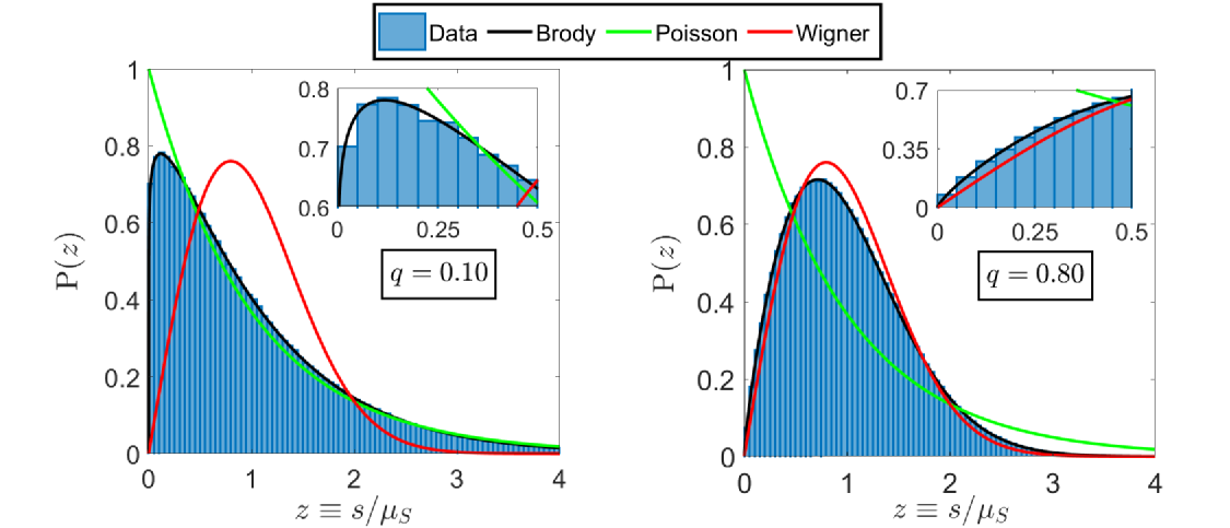
Figure 1: Eigenvalue spacing distributions for $N=10^{6}$ realizations of model $\mathcal{M}^{\text{(II)}}_{B}$ [Eq. (20f)]; values of the Brody parameter $q$ are as indicated. Insets show closer views at small spacings.

VII.2.2 Example 2: Model $\mathcal{M}^{\text{nH}(1)}_{A}$ [Eq. (39)]

Numerical simulations and analyses of model $\mathcal{M}^{\text{nH}(1)}_{A}$ [Eq. (39)], which is complex and non-Hermitian, yield the results shown in Fig. 2; values of the Brody parameter $q$ are as indicated and the value of the scale parameter $\sigma=\sqrt{5}>1$. Numerics and theory are again consistent.

It should be noted that for this model the numerical eigenvalues (as determined by MATLAB’s numerical eigensolver) had tiny imaginary parts (magnitude $<10^{-13}$). These occur as a result of numerical round-off errors. As a numerical fix, $\Lambda_{n}$ in Eq. (48a) was replaced by Re$\{\Lambda_{n}\}$ thereby dropping these spurious imaginary parts.

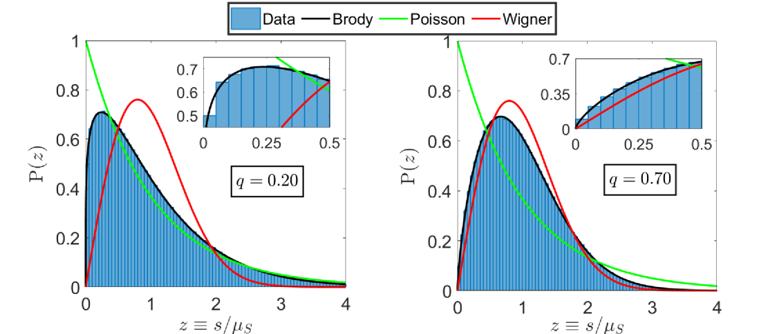
Figure 2: Eigenvalue spacing distributions for $N=10^{6}$ realizations of model $\mathcal{M}^{\text{nH}(1)}_{A}$ [Eq. (39)]; values of the Brody parameter $q$ are as indicated. Insets show closer views at small spacings.

VII.2.3 Example 3: Model $\mathcal{M}^{\text{cs(1)}}_{B}$ [Eq. (42)]

Applying the procedures of Sec. VII.1 to model $\mathcal{M}^{\text{cs(1)}}_{B}$ [Eq. (42)], which is complex and symmetric, yields the results shown in Fig. 3. The value of the scale parameter $\sigma=100$ and constants $\{a(q)=-q,b(q)=q+2\}$ were specifically employed in the simulations. Numerics and theory are once again consistent.

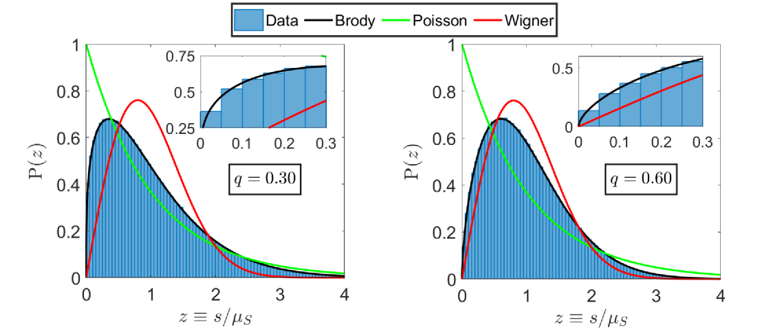
Figure 3: Eigenvalue spacing distributions for $N=10^{6}$ realizations of model $\mathcal{M}^{\text{cs(1)}}_{B}$ [Eq. (42)]; values of the Brody parameter $q$ are as indicated. Insets show closer views at small spacings.

VII.2.4 Example 4: Model $\mathcal{M}^{(\text{sym})}_{A}$ [Eq. (13)] with complex coefficients (47)

As a final example, results are shown in Fig. 4 for model $\mathcal{M}^{(\text{sym})}_{A}$ [Eq. (13)] with complex coefficients given by Eq. (47) and scale parameter $\sigma=1000$. Note that the random matrices in this case are complex-symmetric and possess complex-conjugate eigenvalues (c.f., Example 3 of Sec. VI.2). Numerics and theory are again consistent.

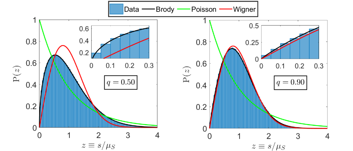
Figure 4: Eigenvalue spacing distributions for $N=10^{6}$ realizations of model $\mathcal{M}^{(\text{sym})}_{A}$ [Eq. (13)] with complex coefficients given by Eq. (47); values of the Brody parameter $q$ are as indicated. Insets show closer views at small spacings.

VIII Comments

VIII.1 Mathematical Comments

Comment M1. The random variables $\left\{Y^{a\over{q+1}},Y^{b\over{q+1}},Y^{c\over{q+1}}\right\}$ appearing in the definition of the general model (6) are (generally) distinct but they are not independent since the numerators $\{a,b,c\}$ of the exponents are necessarily related due to condition (8). The matrix elements are therefore generally dependent; it is in this sense that model (6) is a “correlated” random-matrix model. The net effect of this inherent correlation is that the spacing distribution ends up depending on only the distribution of the root-transformed random variable $Y^{1\over{q+1}}$. Hence, only the distribution of the random variable $Y$ matters. The distribution(s) of any other random variable(s) the exponent(s) could involve (e.g., the variables $U$ and $V$ in $\mathcal{M}^{(\text{asym(2)})}_{A}$ [Eq. (26)]) are immaterial.

Comment M2. Beyond model (6) introduced in this paper, there are many other models that can be constructed that would satisfy condition (8). For example, the $2\times 2$ random-matrix models

$$\mathcal{M}_{1}=\left(\begin{array}[]{cc}\cosh^{2}(X)&{1\over 2}\left(Y^{1\over{q+1}}+1\right)\\ {1\over 2}\left(Y^{1\over{q+1}}-1\right)&\sinh^{2}(X)\end{array}\right),$$ (51c)

$$\mathcal{M}_{2}=\left(\begin{array}[]{cc}\cosh^{2}(X)&{1\over 2}\left(Y^{2\over{q+1}}-1\right)^{1/2}\\ {1\over 2}\left(Y^{2\over{q+1}}-1\right)^{1/2}&\sinh^{2}(X)\end{array}\right),$$ (51f)

where $X$ is independent of $Y$ and can have any arbitrary continuous distribution $f_{X}(x)$, do not derive from model (6) but nonetheless satisfy condition (8), and hence have Brody spacing distributions. Incidentally, the generalizations of Cases I and III of sub-class B given in Sec. IV.1 are also models that are not directly derivable from model (6), but the same comment as above applies to these two cases as well.

Comment M3. Further to Comment M2, the distributions of the individual matrix elements are not fundamentally important for determining the spacing distribution. According to Eq. (28), the distribution of the mixture of random variables that comprise the quantity $\mathcal{D}_{(}\mathcal{M})$ determines the spacing distribution. Thus, the individual matrix elements need not be (linear combinations of) Weibull random variables (with different shape parameters); it is sufficient that the discriminant $\mathcal{D}(\mathcal{M})$ be proportional to the square of a Weibull random variable with shape parameter $\beta=q+1$:

$$\mathcal{D}(\mathcal{M})=kW^{2},~{}~{}k\neq 0,~{}W\sim\text{Weibull}(\sigma,\beta=q+1).$$ (52)

Note that the above condition is a generalization of condition (8). Thus, the general conclusion is that Eq. (35) holds whenever condition (52) is satisfied regardless of the distributions of the individual matrix elements. Interestingly, this means that many different $2\times 2$ random-matrix models will have a Brody spacing distribution.

VIII.2 Physics Comments

Comment P1. In defining the general model (6), the matrices were stipulated to be real but no conditions were imposed that demanded they be symmetric. As discussed in Sec. VI.1, the stipulation that the matrices be real can be relaxed. The interesting consequence is that complex non-Hermitian $2\times 2$ random matrices can have spacing statistics intermediate between Poisson and Wigner. The real-symmetric structure of $2\times 2$ GOE matrices is not required. GOE matrices owe their real and symmetric structure to assumptions and conditions that originate from quantum mechanics. The fact that GOE matrices are symmetric, for example, originally stems from the general assumption that quantum Hamiltonians are Hermitian. This assumption is useful in quantum mechanics since it ensures that all eigenvalues are real, but it is not actually required. In other words, hermiticity is a sufficient but not necessary condition for the eigenvalues to be real. In sub-class A (for example), the eigenvalues are guaranteed to be real by imposition of condition (9d) when the model constants are real or conditions (36) when the constants are complex; hermiticity is not required. Hermiticity is not fundamentally important in the present context due to the small size of the matrices which allows for other tractable (and less restrictive) conditions that can be imposed to ensure the eigenvalues are real; when dealing with large matrices, on the other hand, hermiticity is more imperative. In summary, the complex generalization of model (6) has no built-in quantum-mechanical assumptions or conditions.

Comment P2. The $q=0$ limits of sub-classes A and B generate new classes of $2\times 2$ random-matrix models having Poisson spacing statistics. For example, using (21) with constants $(c_{1}=0,c_{2}=c_{3}=c_{4}={1/2},c_{5}=-{1/2},c_{6}=1)\equiv\mathbf{c}$ and $X\neq 0$, the eigenvalue spacings of the real and non-symmetric random matrix

$$\mathcal{M}^{\text{g(I)}}_{B}(\mathbf{c},q=0)=\left(\begin{array}[]{cc}X&{1\over 2}(Y+V)\\ {1\over 2}(Y-V)&X+V\end{array}\right),~{}~{}~{}$$ (55)

where $\{V\neq 0,X,Y\}$ are independent, will have a Poisson distribution. The $q=0$ sub-classes of models offer a variety of simple $2\times 2$ models that are interesting in the respect that they illustrate that the matrix elements need not be IID nor do any elements need to be Poisson distributed in order for the eigenvalues to have Poissonian spacings. In the above example, none of the matrix elements are Poisson (exponentially) distributed (assuming the distribution of $X$ is not exponential). The matrices need not even be real or Hermitian as the $q=0$ limits of models (39) and (42) illustrate. Non-trivial $2\times 2$ random-matrix models having Poisson spacing statistics are curiously absent in the literature. Interestingly, there does however exist a simple $N\times N$ diagonal model whose eigenvalue spacing distribution converges to Eq. (1) as $N\to\infty$ (see Ref. [61] and references therein).

Comment P3. The $q=1$ limits of sub-classes A and B generate new classes of $2\times 2$ random-matrix models having Wigner spacing statistics. For example, the non-Hermitian matrices

$$\mathcal{M}^{\text{asym}(1)}_{A}(q=1)=\left(\begin{array}[]{cc}X+c_{1}\sqrt{Y}&c_{2}{1\over\sqrt{Y}}\\ c_{3}\sqrt{Y^{3}}&X+c_{4}\sqrt{Y}\end{array}\right)~{}~{}$$ (58)

will (under the condition that $k_{A}\equiv(c_{1}-c_{4})^{2}+4c_{2}c_{3}$ is real and non-zero) have Wigner spacing distributions. The existence of these limit models reinforces the important point that the independence and quantum-mechanical assumptions associated with the construction of the GOE are sufficient but not necessary conditions for the spacing distributions of $2\times 2$ random matrices to be Wignerian. In other words, the elements of a $2\times 2$ random matrix need not be IID nor does the matrix need to be real and/or symmetric in order for its eigenvalues to have a Wigner spacing distribution. A separate and physically important example that illustrates this point can be found in Ref. [62] (see also Ref. [63] for an example of a real and non-symmetric $2\times 2$ random-matrix model having a Wigner spacing distribution). Note furthermore that because the matrix elements are (generally) dependent, they also do not need to be Gaussian distributed (as is the case in Refs. [62, 63]).

IX Conclusion

A class of $2\times 2$ random-matrix models was introduced for which the Brody distribution is the exact eigenvalue spacing distribution. To the author’s knowledge, this is the first class of random matrices that has been found to possess this specific statistical property. Unlike GOE matrices, the matrix elements of this class of random matrices are not IID nor are they Gaussian-distributed. The matrix elements are linear combinations of an exponential random variable raised to different (and possibly variable) powers involving the Brody parameter. The numerators of the exponents are subject only to condition (8) and can otherwise be arbitrarily prescribed. When all exponents are constants, the individual variables that comprise the matrix elements will typically be Weibull random variables with different shape parameters (involving the Brody parameter); exceptions arise when an exponent is not positive-definite (e.g., in model $\mathcal{M}^{\text{(III)}}_{B}$ [Eq. (20i)]), when multiplicative constants are negative, or when there are additional independent random variables whose distributions can be freely prescribed (e.g., the random variable $V$ in model $\mathcal{M}^{\text{g(III)}}_{B}$ [Eq. (22)]). The unconventional nature of the matrix elements are devised as such in order to satisfy the general condition (52).

Real matrices that derive from the general model (6) are not necessarily symmetric. The quantum hermiticity condition, which ensures that all eigenvalues are real, was not imposed in defining the complex generalization of model (6) and is (in the present $2\times 2$ context) a sufficient but not necessary condition for the eigenvalues to be real. As Examples 2-4 in Sec. VII explicitly demonstrate, complex non-Hermitian $2\times 2$ random matrices whose eigenvalues are real (or complex) can possess spacing statistics intermediate between Poisson and Wigner. The author is not aware of any other complex non-Hermitian random-matrix models (or desymmetrized non-Hermitian physical systems) whose real or complex eigenvalues possess such statistics. It is important to emphasize that the classical assumption of IID matrix elements has been dropped in the present model and the question of whether the preceding statement about non-Hermitian matrices holds when the IID assumption is not removed remains open. There are also questions related to pseudo-symmetry [64] and/or pseudo-hermiticity [65] that are pertinent and interesting but such questions are beyond the scope of the present paper.

Finally, as discussed in Comment M3, the individual matrix elements need not be composed of Weibull random variables (with distinct shape parameters) nor even directly involve exponentially-distributed random variables. Thus, there is some flexibility in assigning the matrix elements. The immediate question then is whether other models can be constructed that have varying degrees of non-trivial independence between matrix elements. This is indeed possible; additional independent random variables can be introduced in ways that can reduce the degree of correlation between matrix elements. The author hopes to introduce some classes of semi-correlated bivariate models in a sequel paper.

*

Appendix A The Weibull Distribution

The following can be found in many statistics textbooks (see, for example, Ref. [59]).

Let an arbitrary random variable $W\sim\text{Weibull}(\sigma,\beta)$, that is, let $W$ have a Weibull distribution with scale parameter $\sigma>0$ and shape parameter $\beta>0$. The p.d.f. of $W$ is then given by:

$$f_{W}(w;\sigma,\beta)={\beta\over\sigma}w^{\beta-1}\exp\left(-{w^{\beta}\over\sigma}\right),~{}w\geq 0.$$ (59)

The mean of $W$ is:

$$\mu_{W}(\sigma,\beta)=\left({1\over\sigma}\right)^{-{1/\beta}}\Gamma(1+\beta).$$ (60)

References

- [1] D. Wintgen and H. Friedrich, Phys. Rev. A 35, 1464(R) (1987).
- [2] F. Haake et al., Phys. Rev. A 44, R6161 (1991).
- [3] H.-D. Graf et al., Phys. Rev. Lett. 69, 1296 (1992).
- [4] A. Kudrolli, S. Sridhar, A. Pandey, and R. Ramaswamy, Phys. Rev. E 49, R11 (1994).
- [5] D.M. Leitner, Phys. Rev E 56, 4890 (1997).
- [6] N.-P. Cheng, Z.-Q. Chen, and H. Chen, Chin. Phys. Lett. 19, 309 (2002).
- [7] J. Mur-Petit and R. A. Molina, Phys. Rev E 92, 042906 (2015).
- [8] K. Roy et al., Europhys. Lett. 118, 46003 (2017).
- [9] R. Zhang et al., Chin. Phys. B 28, 100502 (2019).
- [10] P. Sierant and J. Zakrzewski, Phys. Rev. B 99, 104205 (2019).
- [11] M.L. Mehta, Random Matrices, 3rd Ed. (Elsevier, San Diego, 2004).
- [12] F. Haake, Quantum Signatures of Chaos, 3rd ed. (Springer, Berlin, 2010).
- [13] T.A. Brody, Lett. Nuovo Cimento 7, 482 (1973).
- [14] M.V. Berry and M. Robnik, J. Phys. A 17, 2413 (1984).
- [15] E. Caurier, B. Grammaticos, and A. Ramani, J. Phys. A 23, 4903 (1990).
- [16] F.M. Izrailev, J. Phys. A 22, 865 (1989); Phys. Rep. 196, 299 (1990).
- [17] G. Lenz and F. Haake, Phys. Rev. Lett. 67, 1 (1991); G. Lenz, K. Życzkowski, and D. Saher, Phys. Rev. A 44, 8043 (1991).
- [18] T. Prosen and M. Robnik, J. Phys. A 26, 2371 (1993); ibid. 27, L459 (1994); ibid. 27, 8059 (1994).
- [19] E.B. Bogomolny, U. Gerland, and C. Schmit, Phys. Rev. E 59, R1315 (1999); Eur. Phys. J. B 19, 121 (2001).
- [20] T.A. Brody et al., Rev. Mod. Phys. 53, 385 (1981).
- [21] J.M.G. Gómez et al., Phys. Rep. 499, 103 (2011).
- [22] H.-J. Stöckmann, Quantum Chaos: An Introduction (Cambridge University Press, Cambridge, 1999).
- [23] M. Robnik, Nonlin. Phenom. Complex Syst. (Minsk) 23, 172 (2020).
- [24] L.E. Reichl, The Transition to Chaos: Conservative Classical and Quantum Systems, 3rd Ed. (Springer, Switzerland, 2021).
- [25] J.A. Méndez-Bermúdez et al., Phys. Rev. E 91, 032122 (2015).
- [26] C.P. Dettmann, O. Georgiou, and G. Knight, Europhys. Lett. 118, 18003 (2017).
- [27] C. Sarkar and S. Jalan, Chaos 28, 102101 (2018).
- [28] T. Raghav and S. Jalan, Physica A 586, 126457 (2022).
- [29] R. Potestio, F. Caccioli, and P. Vivo, Phys. Rev. Lett. 103, 268101 (2009).
- [30] E.F.N. Santos, A.L.R. Barbosa, and P.J. Duarte-Neto, Phys. Lett. A 384, 126689 (2020).
- [31] Z. Saleki, A.J. Majarshin, Y.-A. Luo, and D.-L. Zhang, Phys. Rev. E 104, 014116 (2021).
- [32] M. Abdel-Mageed, A. Salim, W. Osamy, and A.M. Khedr, Adv. Math. Phys. 2021, 9956518 (2021).
- [33] J.K. Yao, C.A. Johnson, N.P. Mehta, and K.R.A. Hazzard, Phys. Rev. A 104, 053311 (2021).
- [34] T. Araújo Lima, R.B. do Carmo, K. Terto, and F.M. de Aguiar, Phys. Rev. E 104, 064211 (2021).
- [35] S. Behnia, F. Nemati, and M. Yagoubi-Notash, Eur. Phys. J. Plus 137, 347 (2022).
- [36] T. Guhr, A. Müller-Groeling, and H.A. Weidenmüller, Phys. Rep. 299, 189 (1998).
- [37] J.M. Nieminen and L. Muche, Acta Phys. Pol. B 48, 765 (2017).
- [38] G.W. Anderson and O. Zeitouni, Commun. Pure Appl. Math 61, 1118 (2008).
- [39] A. Chakrabarty, R.S. Hazra, and D. Sarkar, Acta Phys. Pol. B 46, 1637 (2015).
- [40] G. Ben Arous and A. Guionnet, in The Oxford Handbook of Random Matrix Theory, edited by G. Akemann, J. Baik, and P. Di Francesco (Oxford University Press, Oxford, 2015).
- [41] O.H. Ajanki, L. Erdős, and T. Krüger, Probab. Theory Relat. Fields 169, 667 (2017).
- [42] S. Chatterjee, Ann. Probab. 34, 2061 (2006).
- [43] K. Hofmann-Credner and M. Stolz, Electron. Commun. Probab. 13, 401 (2008).
- [44] L. Erdős, H.-T. Yau, and J. Yin, Probab. Theory Relat. Fields 154, 341 (2012).
- [45] F. Götze, A.A. Naumov, and A.N. Tikhomirov, Theory Probab. Appl. 59, 23 (2015).
- [46] A.A. Naumov, J. Math. Sci. 204, 140 (2015).
- [47] R. Adamczak, D. Chafaï, and P. Wolff, Rand. Struct. Alg. 48, 454 (2016).
- [48] Z. Che, Electron. J. Probab. 22, 30 (2017).
- [49] O.H. Ajanki, L. Erdős, and T. Krüger, Probab. Theory Relat. Fields 173, 293 (2019).
- [50] L. Peroncelli, G. Grossi, and V. Aquilanti, Molec. Phys. 102, 2345 (2004).
- [51] H. Yang, F. Zhao, and B. Wang, Physica A 364, 544 (2006).
- [52] F.W.K. Firk and S.J. Miller, Symmetry 1, 64 (2009).
- [53] J. Sakhr and J.M. Nieminen, Phys. Rev. E 73, 036201 (2006).
- [54] G. Orjubin, E. Richalot, O. Picon, and O. Legrand, IEEE Trans. Electromagn. Compat. 49, 762 (2007).
- [55] J.-B. Gros et al., Wave Motion 51, 664 (2014).
- [56] H. Matsumura, Commutative Ring Theory (Cambridge University Press, Cambridge, 1989).
- [57] A.B. Jaiswal, A. Pandey, and R. Prakash, Europhys. Lett. 127, 30004 (2019).
- [58] G. Akemann, A. Mielke, and P. Päler, Phys. Rev. E 106, 014146 (2022).
- [59] N.L. Johnson, S. Kotz, and N. Balakrishnan, Continuous Univariate Distributions: Volume 1, 2nd Ed. (Wiley, New York, 1994).
- [60] M.V. Berry and P. Shukla, J. Phys. A 42, 485102 (2009).
- [61] A.A. Abul-Magd and A.Y. Abul-Magd, Alex. J. Phys. 1, 65 (2011).
- [62] Z. Ahmed, Phys. Lett. A 308, 140 (2003).
- [63] S. Grossmann and M. Robnik, J. Phys. A 40, 409 (2007).
- [64] S. Kumar and Z. Ahmed, Phys. Rev. E 96, 022157 (2017).
- [65] J. Feinberg and R. Riser, J. Phys.: Conf. Ser. 2038, 012009 (2021).