Timelike geodesics for five-dimensional Schwarzschild and Reissner-Nordström Anti-de Sitter black holes

Abstract

The timelike structure of the five–dimensional Schwarzschild and Reissner-Nordström Anti-de Sitter black holes is studied in detail. Different kinds of motion are allowed and studied by using an adequate effective potential. Then, by solving the corresponding equations of motion, several trajectories and orbits are described in terms of Weierstraß  elliptic functions and elementary functions for neutral particles.

1 Introduction

The study of the gravitation in higher dimensional space-times has been widely considered since the revolutionary ideas of Kaluza and Klein Kaluza21 ; Klein26 , where it was intended to unify electromagnetic theory with the also revolutionary Einstein’s theory of general relativity, to the modern ideas of string theory, where the action contains terms that appear as corrections to the Einstein-Hilbert action Font:2005td ; Chan:2000ms . In this sense, the vacuum solutions of general relativity for five dimensional, static, spherically symmetric black hole, known as the Schwarzschild-Tangherlini black holes solution, was obtained in Ref. Tangherlini:1963bw , and represents the starting point for the study of more general five dimensional space-times. In particular, the Reissner-Nordström anti-de Sitter (RNAdS) black hole solution posses interesting features in the context of the AdS/CFT correspondence Maldacena:1997re ; Witten:1998qj ; Gubser:1998bc , and other realizations Friess:2006kw ; Saadat:2012zza ; Villanueva:2013zta ; Gonzalez:2020zfd . The properties of Reissner-Nordström black hole in $d$-dimensional anti-de Sitter space-time has been studied in Refs. Chamblin:1999tk ; Chamblin:1999hg , and some studies of geodesics of test particles in higher dimensional black hole spacetimes has been analyzed in Refs. Kovacs:1984qx ; PhysRevLett.98.061102 ; Seahra:2001bx ; Frolov:2003en ; Hackmann:2008tu ; Guha:2010dd ; Gibbons:2011rh ; Guha:2012ma ; Kagramanova:2012hw ; Chandler:2015aha ; Gonzalez:2015qxc ; Grunau:2017uzf ; Kuniyal:2017dnu . Also, interesting aspects of the thermodynamic of higher dimensional black holes can be studied following the Refs. Fernandes ; andre ; kong .

In this work we have extended the study of the geodesic structure of the five-dimensional RNAdS black hole that we carried out in Gonzalez:2020zfd , where the null structure of such black hole was studied in detail, finding, among other things, new classes of orbits, genuine of this space-time, as the hippopede of Proclus geodesic. It is worth to mention that the thermodynamics and the stability of the spacetime under consideration were studied via a thermodynamic point of view, and it was found special conditions on the black hole mass and the black hole charge where the black hole is in a stable phase Saadat:2012zza . Also, the radial and circular motion of massive particles for this spacetime was analized in Ref. Guha:2010dd , where the geodesics were studied from the point of view of the effective potential formalism and the dynamical systems approach. Finally, the shadow of the five-dimensional RN AdS black hole was studied in Ref. Mandal:2022oma .

The manuscript is organized as follows: in Sec. 2 we briefly review the main aspects of the spacetime under consideration present the bases of spacetime under consideration. Then, in Sec. 3, we solve the (time-like) geodesic equation and study in detail the different orbits for neutral particles. Finally, conclusions and final remarks are presented in Sec. 4.

2 Five-dimensional Schwarzschild and Reissner-Nordström anti-de Sitter black hole

The five-dimensional RNAdS black hole is a solution of the field equations that arise from the action Chamblin:1999hg

$$S=-\frac{1}{16\pi G_{5}}\int d^{5}x\sqrt{-g}(R-2\Lambda-F^{2})\,,$$ (1)

where $G_{5}$ is the 5-dimensional gravitational constant, $R$ is the Ricci scalar, $F^{2}$ represents the electromagnetic Lagrangian, $\Lambda=-6/\ell^{2}$ is the cosmological constant, and $\ell$ is the radius of AdS₅ space. The static, spherically symmetric metric that solves the field equations is given by

$${\rm d}s^{2}=-f(r)\,{\rm d}t^{2}+\frac{1}{f(r)}{\rm d}r^{2}+r^{2}\,{\rm d}\Omega_{3}^{2}\,,$$ (2)

where the lapse function $f(r)$ is given by

$$f(r)=1-\frac{4M^{2}}{r^{2}}+\frac{Q^{4}}{r^{4}}+\frac{r^{2}}{\ell^{2}}\,,$$ (7)

and ${\rm d}\Omega_{3}^{2}={\rm d}\theta^{2}+\sin^{2}\theta\,{\rm d}\phi^{2}+\sin^{2}\theta\,\sin^{2}\phi\,{\rm d}\psi^{2}$ is the metric of the unit 3-sphere.

This spacetime allows an event horizon $r_{+}$, and a Cauchy horizon $r_{-}$, obtained from the equation $f(r)=0$, which leads to the sixth degree polynomial

$$P(r)\equiv r^{6}+\ell^{2}\,r^{4}-4M^{2}\ell^{2}\,r^{2}+\ell^{2}Q^{4}=0\,.$$ (8)

The change of variable $x=r^{2}-\ell^{2}/3$ allows to write Eq. (8) as $P(x)=x^{3}-\alpha x+\beta$, where

$$\alpha=\ell^{2}\left(4M^{2}+\frac{\ell^{2}}{3}\right),\,\,\,\beta=\ell^{2}\left(Q^{4}+\frac{4M^{2}\ell^{2}}{3}+\frac{2\,\ell^{4}}{27}\right),$$ (9)

therefore, the Cauchy and the event horizons can be written as

$$r_{-}=\sqrt{x_{0}-\ell^{2}/3},\quad r_{+}=\sqrt{x_{1}-\ell^{2}/3}\,,$$ (10)

where $x_{n}=Z\sin\left(\Theta+2n\pi/3\right)$, $Z=2\sqrt{\alpha/3}$ and
$\Theta=\frac{1}{3}\arcsin\left(\frac{3\sqrt{3}\beta}{2\alpha^{3/2}}\right)$. The extremal black hole is characterized by the condition $r_{ext}=r_{+}=r_{-}$, obtained from the relation

$$4\ell^{4}\left(4M^{2}-Q^{2}\right)+8\ell^{2}M^{2}\left(32M^{4}-9Q^{4}\right)-27Q^{8}=0\,.$$ (11)

Note that when $Q=0$, the lapse function reduces to the five-dimensional Schwarzschild anti-de Sitter black hole, and the spacetime allows one horizon (the event horizon $r_{+}$) given by

$$r_{+}=\ell\,\sinh\left[{1\over 2}\mathrm{arcsinh}\left({4M\over\ell}\right)\right]\,.$$ (12)

3 The timelike structure for neutral particles

In order to obtain a description of the allowed motion in the exterior spacetime of the black hole, we use the standard Lagrangian formalism Chandrasekhar:579245 ; Cruz:2004ts ; Villanueva:2018kem , so that, the corresponding Lagrangian associated with the line element (2) reads

$$\mathcal{L}=-\frac{f(r)\,\dot{t}^{2}}{2}+\frac{\dot{r}^{2}}{2f(r)}+\frac{r^{2}}{2}\mathcal{L}_{\Omega}\,,$$ (13)

where $\mathcal{L}_{\Omega}$ is the angular Lagrangian:

$$\mathcal{L}_{\Omega}=\dot{\theta}^{2}+\sin^{2}\theta\,\dot{\phi}+\sin^{2}\theta\,\sin^{2}\phi\,\dot{\psi}^{2}\,.$$ (14)

Here, the dot indicates differentiation with respect to the proper time $\tau$. Since the Lagrangian (13) does not depend on the coordinates ($t,\psi$), they are cyclic coordinates and, therefore, the corresponding conjugate momenta $\pi_{q}=\partial\mathcal{L}/\partial\dot{q}$ is conserved along the geodesic. Explicitly, we have

$$\pi_{t} = -f(r)\,,\,\,\dot{t}\equiv-E\,,$$ (15)

$$\pi_{\psi} = r^{2}\sin^{2}\theta\sin^{2}\phi\,\dot{\psi}=L\,,$$ (16)

where $E$ is a positive constant that depicts the time invariance of the Lagrangian, which cannot be associated with energy because the spacetime defined by the line element (2) is not asymptotically flat, whereas the constant $L$ stands the conservation of angular momentum, under which it is established that the motion is performed in an invariant hyperplane. Here, we claim to study the motion in the invariant hyperplane $\theta=\phi=\pi/2$, so $\dot{\theta}=\dot{\phi}=0$ and, from Eq. (16), we obtain

$$\dot{\psi}=\frac{L}{r^{2}}\,.$$ (17)

Therefore, using the fact that $2\mathcal{L}=-1$ for particles together with Eqs. (15) and (17), we obtain the following equations of motion

$$\left(\frac{{\rm d}r}{{\rm d}\lambda}\right)^{2}=E^{2}-V^{2}(r)\,,$$ (18)

$$\left(\frac{{\rm d}r}{{\rm d}t}\right)^{2}={f^{\,2}(r)\over E^{2}}\left[E^{2}-V^{2}(r)\right]\,,$$ (19)

$$\left(\frac{{\rm d}r}{{\rm d}\psi}\right)^{2}={r^{\,4}\over L^{2}}\left[E^{2}-V^{2}(r)\right]\,,$$ (20)

where the effective potential $V^{2}(r)$ is defined by

$$V^{2}(r) \equiv f(r)\left[1+\frac{L^{2}}{r^{2}}\right]=1-\frac{4M^{2}}{r^{2}}+\frac{Q^{4}}{r^{4}}+\frac{r^{2}}{\ell^{2}}+$$ (21)

$$+\frac{L^{2}}{\ell^{2}}+\frac{L^{2}}{r^{2}}-\frac{4M^{2}L^{2}}{r^{4}}+\frac{Q^{4}L^{2}}{r^{6}}\,.$$

The behaviour of the effective potential is plotted in Fig. 1, for test particles with angular momentum. Note that the following orbits are allowed: there are second kind trajectories for $0<L<L_{\text{LSCO}}$, there are last stable circular orbits (LSCO) and second kind trajectories for $L=L_{\text{LSCO}}$, and there are planetary orbits, circular orbits (stable and unstable) and second kind of trajectories for $L>L_{\text{LSCO}}$. While that for the motion with $L=0$, see Fig. 2, there are second kind trajectories. Note that the effect of the black hole charge is the existence of a return point located at $r<r_{-}$.

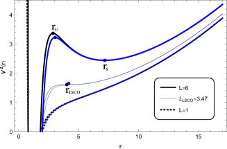
Figure 1: The behaviour of the effective potential of neutral particles as a function of $r$ for different values of the angular momentum. Here, we have used the values $M=1$, $\ell=10$, $Q=1.2$ (black lines), and $Q=0$ (blue lines). For $Q=1.2$, the unstable circular orbit occurs at $r_{U}=2.86$, the stable circular orbit at $r_{S}=7.18$, and the last stable circular orbit at $r_{\text{LSCO}}=4.01$, while that for $Q=0$ the unstable/stable/last stable circular orbits occurs at $r_{U}=3.04$, $r_{S}=7.17$ and $r_{\text{LSCO}}=4.16$, respectively.

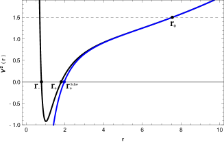
Figure 2: The behaviour of the effective potential $V^{2}(r)$ for the motion of particles with $L=0$, $M=1$, and $\ell=10$. Black line for $Q=1.2$ ($r_{0}\approx 7.547$), and blue line for $Q=0$ ($r_{0}\approx 7.551$). Here, $r_{-}\approx 0.783$, $r_{+}\approx 1.805$, and $r_{+}^{\text{Schw}}\approx 1.963$.

In the next subsections, we will study the motion of neutral particles in five-dimensional backgrounds. Firstly, we will consider Schwarzschild black holes as uncharged spacetimes, and Reissner-Nordström black holes, as charged spacetimes.

3.1 Five-dimensional Schwarzschild black hole

In this section, firstly we will study the confined orbits, that is, circular and planetary orbits. Then, we will study the unconfined orbits, as second kind, and critical trajectories, and finally the motion of particles with vanishing angular momentum.

3.1.1 Circular orbits

The existence of a maximum and a minimum in the potential corresponds to unstable (U)/stable(S) circular orbits, respectively. Thus, $V^{\prime}=0$ yields

$$\tilde{P}(r)\equiv r^{6}-\tilde{A}r^{2}+\tilde{B}=0\,,$$ (22)

where $\tilde{A}=\ell^{2}(L^{2}-4M^{2})$, and $\tilde{B}=8\ell^{2}L^{2}M^{2}$. Thereby, the particles can stay in unstable (stable) circular orbits of radius $r_{U}$ ($r_{S}$), given by

$$r_{U}=\left[\sqrt{\frac{4\tilde{A}}{3}}\cos\left(\frac{1}{3}\cos^{-1}\left(-12\tilde{B}\sqrt{\frac{3}{(4\tilde{A})^{3}}}\right)+\frac{4\pi}{3}\right)\right]^{1/2}\,,\\$$ (23)

$$r_{S}=\left[\sqrt{\frac{4\tilde{A}}{3}}\cos\left(\frac{1}{3}\cos^{-1}\left(-12\tilde{B}\sqrt{\frac{3}{(4\tilde{A})^{3}}}\right)\right)\right]^{1/2}\,.$$ (24)

Now, in order to determine the analytical value of $L_{LSCO}$, where $r_{U}=r_{S}=r_{LSCO}$, we set to zero the discriminant $\Delta$ of Eq. (22) given by $\Delta=4\tilde{A}^{3}-27\tilde{B}^{2}$, which yields

$$L^{6}-L^{4}\left(\frac{432M^{4}}{\ell^{2}}+12M^{2}\right)+48L^{2}M^{4}-64M^{6}=0\,.$$ (25)

Therefore,

$$L_{LSCO}=\sqrt{z_{0}+\frac{144M^{4}}{\ell^{2}}+4M^{2}}\,,$$ (26)

where

$$z_{0}=\sqrt{\frac{h_{2}}{3}}\cosh\left(\frac{1}{3}\cosh^{-1}\left(3\sqrt{\frac{3}{h_{2}^{3}}}h_{3}\right)\right)\,,$$ (27)

$$h_{2}=\frac{4\left(3456M^{6}\left(\ell^{2}+18M^{2}\right)\right)}{\ell^{4}}\,,$$ (28)

$$h_{3}=\frac{4\left(6912M^{8}\left(\ell^{4}+864M^{4}+72\ell^{2}M^{2}\right)\right)}{\ell^{6}}\,.$$ (29)

In Fig. 3, we show the behaviour of the effective potential when the angular momentum increases. By using Eqs. (23), and (24) we obtain that $\lim_{L\to\infty}r_{U}=2\sqrt{2}M$, and $\lim_{L\to\infty}r_{S}=+\infty$, which is shown in Fig. 3 for $M=1$.

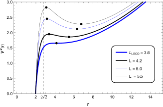
Figure 3: The effective potential of Schwarzschild black hole for different values of the angular momentum $L$, with $M=1$, and $\ell=10$. Here, $r_{\text{LSCO}}=4.16$ for $L_{LSCO}=3.6$. Note that when the angular momentum increases, the radius of the unstable circular orbit tends to $2\sqrt{2}$, while that the radius of the stable circular orbit increases.

On the other hand, the proper period in such circular orbit of radius $r_{c.o.}$ is

$$T_{\tau}=2\pi\,r_{c.o.}\ell\,\sqrt{\frac{r_{c.o.}^{2}-8M^{2}}{r_{c.o.}^{4}+4M^{2}\ell^{2}}}\,,$$ (30)

and the coordinate period is

$$T_{t}=\frac{2\pi r^{2}_{c.o.}\ell}{\sqrt{r_{c.o.}^{4}+4\ell^{2}M^{2}}}\,.$$ (31)

Now, in order to obtain the epicycle frequency for the stable circular orbit we expand the effective potential around $r=r_{S}$, which yields

$$V(r)=V(r_{S})+V^{\prime}(r_{S})(r-r_{S})+{1\over 2}V^{\prime\prime}(r_{S})(r-r_{S})^{2}+...\,,$$ (32)

where$\,{}^{\prime}$ means derivative with respect to the radial coordinate. Obviously, in this orbits $V^{\prime}(r_{S})=0$. So, by defining the smaller coordinate $x=r-r_{S}$, together with the epicycle frequency $\kappa^{2}\equiv 1/2V^{\prime\prime}(r_{S})$ RamosCaro:2011wx , we can rewrite the above equation as

$$V(x)\approx E_{S}^{2}+\kappa^{2}\,x^{2}\,,$$ (33)

where ${E_{S}}$ is the energy of the particle at the stable circular orbit. Also, it is forward to see that the test particles satisfy the harmonic equation of motion $\ddot{x}=-\kappa^{2}\,x$, and the epicycle frequency is given by

$$\kappa^{2}=\frac{4\left(-16\ell^{2}M^{4}-12M^{2}r_{S}^{4}+r_{S}^{6}\right)}{\ell^{2}r_{S}^{4}\left(r_{S}^{2}-8M^{2}\right)}\,.$$ (34)

3.1.2 Planetary orbits

As mentioned, the planetary orbits are orbits of the first kind, and they occur when $L>L_{LSCO}$, and the energy $E$ lies in the range $E_{S}<E<E_{U}$. Thus, we can rewrite the characteristic polynomial as

$$\left(\ell\,L\,\frac{{\rm d}r}{{\rm d}\psi}\right)^{2}=-\mathcal{P}(r)=-(r^{6}+\tilde{a}r^{4}+\tilde{b}r^{2}+\tilde{c})\,,$$ (35)

where $\tilde{a}=-\ell^{2}(E^{2}-1-L^{2}/\ell^{2})$, $\tilde{b}=-\ell^{2}(4M^{2}-L^{2})$, $\tilde{c}=-\ell^{2}\left(4L^{2}M^{2}\right)$. So, $\mathcal{P}(r)=0$ allows three real positive roots, which we can identify as: $r_{P}$, it corresponds to a periastro distance, $r_{A}$ is interpreted as a apoastro distance, and $r_{F}$ is a turning point for the second kind trajectories. Thereby, the polynomial (35) can be written as

$$\mathcal{P}(r)=\left(r^{2}-r_{A}^{2}\right)(r^{2}-r^{2}_{P})(r^{2}-r_{F}^{2})\,,$$ (36)

where the return points are given by

$$r_{A} = \left[u_{0}-\frac{1}{3}\left(-\ell^{2}E^{2}+\ell^{2}+L^{2}\right)\right]^{1/2}\,,$$ (37)

$$r_{P} = \left[u_{2}-\frac{1}{3}\left(-\ell^{2}E^{2}+\ell^{2}+L^{2}\right)\right]^{1/2}\,,$$ (38)

$$r_{F} = \left[u_{1}-\frac{1}{3}\left(-\ell^{2}E^{2}+\ell^{2}+L^{2}\right)\right]^{1/2}\,,$$ (39)

and the constants are

$$u_{n} = \sqrt{{\tilde{\eta}_{2}\over 3}}\cos\left(\frac{1}{3}\arccos\left({3}\tilde{\eta}_{3}\sqrt{{3\over\tilde{\eta}_{2}^{3}}}\right)+\frac{2\pi n}{3}\right)\,,$$ (41)

$$\tilde{\eta}_{2} = \frac{4}{3}\left(\ell^{4}\left(E^{2}-1\right)^{2}+L^{4}-\ell^{2}L^{2}\left(2E^{2}+1\right)\right.$$ (42)

$$\left.+12\ell^{2}M^{2}\right)\,,$$

$$\tilde{\eta}_{3} = -4\left(\frac{2}{27}\left(L^{2}-\ell^{2}\left(E^{2}-1\right)\right)^{3}-4\ell^{2}L^{2}M^{2}\right.$$ (43)

$$\left.-\frac{1}{3}\ell^{2}\left(L^{2}-4M^{2}\right)\left(L^{2}-\ell^{2}\left(E^{2}-1\right)\right)\right)\,.$$

Therefore, the solution of planetary geodesics is given by

$$r(\phi)=\frac{r_{A}}{\sqrt{4\wp(\kappa_{P}\phi+\varphi_{P})+\kappa_{2}}}\,,$$ (44)

where the integration constants are

$$\varphi_{P}=\wp^{-1}\left(\frac{1-\kappa_{2}}{4}\right)\,,$$ (45)

$$\kappa_{2}=\frac{1}{3}\left(1+\left(\frac{r_{A}}{r_{F}}\right)^{2}+\left(\frac{r_{A}}{r_{P}}\right)^{2}\right)\,,\,\,\kappa_{p}=\frac{2r_{P}r_{F}}{\ell L}\,,$$ (46)

and the Weierstra$\ss$ invariants are

$$g_{2} = \frac{1}{12}\left(-\left(\frac{r_{A}}{r_{F}}\right)^{2}\left(\frac{r_{A}}{r_{P}}\right)^{2}+\left(\frac{r_{A}}{r_{F}}\right)^{4}-\left(\frac{r_{A}}{r_{F}}\right)^{2}\right.$$ (47)

$$\left.+\left(\frac{r_{A}}{r_{P}}\right)^{4}-\left(\frac{r_{A}}{r_{P}}\right)^{2}+1\right)\,,$$

$$g_{3} = \frac{1}{432}\left(\left(\frac{r_{A}}{r_{F}}\right)^{2}-2\left(\frac{r_{A}}{r_{P}}\right)^{2}+1\right)\times$$

$$\left(2\left(\frac{r_{A}}{r_{F}}\right)^{2}-\left(\frac{r_{A}}{r_{P}}\right)^{2}-1\right)\left(\left(\frac{r_{A}}{r_{F}}\right)^{2}+\left(\frac{r_{A}}{r_{P}}\right)^{2}-2\right)\,.$$

Also, the solution (44), allows us to determine the precession angle $\Theta$, by considering that it is given by $\Theta=2\phi_{P}-2\pi$, where $\phi_{P}$ is the angle from the apoastro to the periastro. Thus, we obtain

$$\Theta=\frac{2}{\kappa_{P}}\left(\wp^{-1}\left(\frac{r_{A}^{2}}{4r_{P}^{2}}-\frac{\kappa_{2}}{4}\right)-\wp^{-1}\left(\frac{1}{4}-\frac{\kappa_{2}}{4}\right)\right)-2\pi\,.$$ (49)

This an exact solution for the angle of precession, and it depends on the spacetime parameters and on the particle motion constants. So, according with Eq. (49), in Fig. 4, we show the behaviour of the precession angle $\Theta$ as a function of the energy $E$, where the precession is negative for $E_{s}<E<E_{0}$, the precession is null for $E=E_{0}$, and it is positive for $E_{0}<E<E_{U}$, which we show in Fig. 5, via Eq. (44).

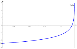
Figure 4: The behaviour of the precession angle $\Theta$ as a function of the energy $E$, with $M=1$, $\ell=10$, and $L=6$. Note that the precession angle vanishes when $E=E_{0}\approx 1.789$, it tends to infinity when $E\rightarrow E_{U}\approx 1.797$, and $\Theta\rightarrow\Theta_{S}\approx-2.424$ when the energy $E\rightarrow E_{S}\approx 1.563$.

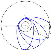
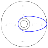
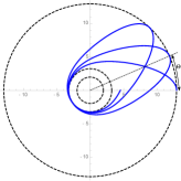
Figure 5: The behaviour of second kind trajectories with $M=1$, $\ell=10$, and $L=6$. Top panel corresponds to an orbit with negative precession $E\approx 1.74$, central panel without precession with $E\approx 1.790$, and bottom panel for a positive precession with $E\approx 1.799$.

3.1.3 Second kind trajectories

The particles describe second kind trajectories when they start from a point of the spacetime and then they plunge into the horizon. In Fig. 6, we show such trajectories. In the top panel, we observe that analytical extension of the geodesics show a similar trajectory to the cardioid Cruz:2004ts .

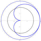
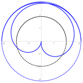
Figure 6: The behaviour of second kind trajectories with $M=1$, $\ell=10$, and $L=6$. Top panel corresponds to a orbit without precession with $E\approx 1.790$, central panel for a positive precession with $E\approx 1.799$, and bottom panel for negative precession $E=1.74$. The small circle represents to the event horizon, while that the bigger circle represents to the return point $r_{F}$.

An analytical solution for second kind trajectories described by elementary functions can be found when $E=E_{S}$, and it is given by

$$r_{2K}(\phi)=\frac{r_{F}r_{S}}{\sqrt{r_{S}^{2}+\left(r_{S}^{2}-r_{F}^{2}\right)\tan(\frac{r_{S}\sqrt{r_{S}^{2}-r_{F}^{2}}}{\ell L_{P}}\phi)^{2}}}\,.$$ (50)

In Fig. 7, we plot the above solution and we can see a special second kind trajectory with a negative precession.

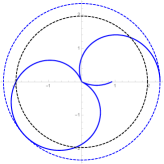
Figure 7: The behaviour of a special second kind trajectories with $M=1$, $\ell=10$, $L=6$, and $E=E_{S}=1.563$. The small circle represents to the event horizon $r_{H}\approx 1.963$, while that the bigger circle represents to the return point $r_{F}=2.5$. Here, $r_{S}\approx 6.325$.

3.1.4 Critical trajectories

This kind of motion is indeed ramified into two cases; critical trajectories of the first kind (CFK) in which the particles come from a distant position $r_{0}$ to $r_{U}$ and those of the second kind (CSK) where the particles start from an initial point near the horizon and can plunge into the horizon or they can tend to the stable circular orbit by spiraling. We obtain the following equations of motion for the aforementioned trajectories:

$$r_{CFK}(\phi)=\frac{R_{0}r_{U}}{\sqrt{\left(R_{0}^{2}-r_{U}^{2}\right)\tanh^{2}(k_{1}\phi)+r_{U}^{2}}}\,,$$ (51)

$$r_{CSK}(\phi)=\frac{R_{0}r_{U}}{\sqrt{\left(R_{0}^{2}-r_{U}^{2}\right)\tanh^{2}(k_{1}\phi+\varphi_{2})+r_{U}^{2}}}\,,$$ (52)

where $\kappa_{1}=\frac{R_{0}\sqrt{R_{0}^{2}-r_{U}^{2}}}{\ell L}$, $\varphi_{2}=\tanh^{-1}\left(\frac{r_{U}\sqrt{R_{0}^{2}-r_{0}^{2}}}{r_{0}\sqrt{R_{0}^{2}-r_{U}^{2}}}\right)$, and $R_{0}$ is $\left.r_{A}\right|_{E_{U}}$. In Fig. 8, we show the behaviour of the CFK (blue line) and CSK (red line) trajectories, given by Eq. (51) and Eq. (52).

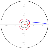
Figure 8: The behaviour of critical trajectories with $M=1$, $\ell=10$, and $L=6$. Blue line for CFK and red line for CSK trajectories with $E=E_{U}\approx 1.797$, and $r_{U}\approx 3.041$. The small dashed circle represents to the event horizon, while that the bigger circle represents to the return point $R_{0}$.

3.1.5 Motion with $L=0$.

For the motion of particles with $L=0$ the effective potential is $V^{2}=f(r)$. Consequently, the equations governing this kind of motion are

$$\frac{dr}{d\tau}=\pm\sqrt{E^{2}-f(r)}\,,$$ (53)

and

$$\frac{dr}{dt}=\pm\frac{f(r)}{E}\,\sqrt{E^{2}-f(r)}\,,$$ (54)

where the $+$ ($-$) sign corresponds to particles moving toward the spatial infinite (event horizon). Now, we consider that the particles are placed at $r=\rho_{0}$ when $t=\tau=0$, which is also a turning point, and it is located at

$$\rho_{0}=\left[{\ell^{2}(1-E^{2})\over 2}+\sqrt{\ell^{4}\left({1-E^{2}\over 2}\right)^{2}+4M^{2}\ell^{2}}\,\right]^{1\over 2}\,.$$ (55)

So, it is possible to obtain the proper time ($\tau$) for the motion of massive particles with $L=0$ in terms of the radial coordinate ($r$), resulting

$$\tau\left(r\right)={\ell\over 2}\left[\sin^{-1}[\Xi(\rho_{0})]-\sin^{-1}[\Xi(r)]\right]\,,$$ (56)

where

$$\Xi(r)={2\,r^{2}+\ell^{2}(1-E^{2})\over\sqrt{16M^{2}\ell^{2}+\ell^{4}(1-E^{2})^{2}}}\,,$$ (57)

and the coordinate time ($t$) as function of $r$ yields

$$t\left(r\right)=\bar{A}_{0}\,\sum_{i=1}^{2}\bar{A}_{i}\,\left[\bar{F}_{i}(r)-\bar{F}_{i}(\rho_{0})\right]\,,$$ (58)

where the functions $\bar{F}_{j}(r)$ ($j=1,2$) are given explicitly by

$$\bar{F}_{1}(r) = \ln\left|\frac{\rho_{0}^{2}-r_{+}^{2}}{r^{2}-r_{+}^{2}}{Y_{1}(r)\over Y_{1}(\rho_{0})}\right|\,,$$ (59)

$$\bar{F}_{2}(r) = \ln\left|\frac{\rho_{0}^{2}+r_{+}^{2}+\ell^{2}}{r^{2}+r_{+}^{2}+\ell^{2}}{Y_{2}(r)\over Y_{2}(\rho_{0})}\right|\,,$$ (60)

where

$$Y_{1}(r) = 2k_{1}-k_{2}(r^{2}-r_{+}^{2})+2\sqrt{k_{1}\,y_{1}(r)}\,,$$ (61)

$$Y_{2}(r) = 2\bar{k}_{1}+\bar{k}_{2}(r^{2}+r_{+}^{2}+\ell^{2})+2\sqrt{\bar{k}_{1}\,y_{2}(r)}\,.$$ (62)

$$y_{1}(r) = k_{1}-k_{2}(r^{2}-r_{+}^{2})-(r^{2}-r_{+}^{2})^{2}\,,$$ (63)

$$y_{2}(r) = \bar{k}_{1}-\bar{k}_{2}(r^{2}+r_{+}^{2}+\ell^{2})-(r^{2}+r_{+}^{2}+\ell^{2})^{2}\,.$$ (64)

with the corresponding constants,

$$\bar{A}_{0}={E\,\ell^{3}\over 2(2r_{+}^{2}+\ell^{2})}\,,\,\,\bar{A}_{1}={r_{+}^{2}\over\sqrt{k_{1}}}\,,\,\,\bar{A}_{2}={r_{+}^{2}+\ell^{2}\over\sqrt{\bar{k}_{1}}}\,,$$ (65)

$$k_{1} = 4M^{2}\ell^{2}-r_{+}^{4}-r_{+}^{2}\ell^{2}(1-E^{2})\,,$$ (66)

$$k_{2} = 2r_{+}^{2}+\ell^{2}(1-E^{2})\,,$$ (67)

$$\bar{k}_{1} = 4M^{2}\ell^{2}-(r_{+}^{2}+\ell^{2})^{2}-(r_{+}^{2}+\ell^{2})\ell^{2}(1-E^{2})\,,$$ (68)

$$\bar{k}_{2} = 2(r_{+}^{2}+\ell^{2})-\ell^{2}(1-E^{2})\,.$$ (69)

Now, in order to visualize the behaviours of the proper and coordinate time, we plot in Fig 9, their behaviours via the solution (56), and (58), respectively. It is possible to observe that the particles moving to the event horizon, $r_{+}$, cross it in a finite proper time ($\tau$), but an external observer will see that the particles take an infinite (coordinate) time ($t$) to do it.

Figure 9: Proper and coordinate time as a function of $r$ for the motion with $L=0$ of test particles. Here, we have used the values $E\approx 0.707$, and $\rho_{0}\approx 2.649$ (thin curve), $E=1$, and $\rho_{0}\approx 4.472$ (thick curve), with $M=1$, $\ell=10$. The dashed line corresponds to the event horizon ($r_{+}\approx 1.963$).

3.2 Five-dimensional Reissner-Nordström black hole

Now, for a charged spacetime, as previosly, firstly we will study the confined orbits, that is, circular and planetary orbits. Then, we will study the unconfined orbits, as the second kind, and critical trajectories, and finally the motion of particles with vanishing angular momentum.

3.2.1 Circular orbits.

Similar to the previous background, we find two types of circular orbits. Thus, the particles can stay in an unstable (stable) circular orbit of radius $r_{U}$ ($r_{S}$), that can be obtained doing, $V^{\prime}=0$. So,

$$\bar{P}(r)\equiv r^{8}+\bar{A}r^{4}+\bar{B}r^{2}+\bar{C}=0\,,$$ (70)

where $\bar{A}=\ell^{2}(4M^{2}-L^{2})$, $\bar{B}=\ell^{2}\left(8L^{2}M^{2}-2Q^{4}\right)$, and $\bar{C}=-3\ell^{2}L^{2}Q^{4}$. This eighth degree polynomial can be reduced to a fourth degree polynomial, where the radius are given by

$$r_{U} = \left[\bar{\alpha}+\sqrt{\bar{\alpha}^{2}-\bar{\beta}}\right]^{1/2}\,,$$ (71)

$$r_{S} = \left[\bar{\alpha}-\sqrt{\bar{\alpha}^{2}-\bar{\beta}}\right]^{1/2}\,,$$ (72)

and the constants of the solution are

$$\bar{\alpha}=\left[\bar{U}-{\bar{A}\over 6}\right]^{1/2}\,,\,\,\bar{\beta}=2\bar{\alpha}^{2}+{\bar{A}\over 2}+{\bar{B}\over 4\bar{\alpha}}\,,$$ (73)

$$\bar{U}=2\sqrt{{\bar{\eta}_{2}\over 3}}\cosh\left(\frac{1}{3}\mathrm{arccosh}\left({3\over 2}\bar{\eta}_{3}\sqrt{{3\over\bar{\eta}_{2}^{3}}}\right)\right)\,,$$ (74)

$$\bar{\eta}_{2}={\bar{A}^{2}\over 48}+{\bar{C}\over 4}\,,\,\,\bar{\eta}_{3}={\bar{A}^{3}\over 864}+{\bar{B}^{2}\over 64}-{\bar{A}\bar{C}\over 24}\,.$$ (75)

The affine period in such circular orbit of radius $r_{c.o.}$ is

$$T_{\tau}=2\pi\,r_{c.o.}\ell\,\sqrt{\frac{r_{c.o.}^{4}-8M^{2}r_{c.o.}^{2}+3Q^{4}}{r_{c.o.}^{6}+4\ell^{2}M^{2}r_{c.o.}^{2}-2\ell^{2}Q^{4}}}\,,$$ (76)

and the coordinate period is

$$T_{t}=\frac{2\pi\,r_{c.o.}^{3}\,\ell}{\sqrt{r_{c.o.}^{6}+4\ell^{2}M^{2}r_{c.o.}^{2}-2\ell^{2}Q^{4}}}\,.$$ (77)

So, when the black hole charge is null, we recover the periods obtained for Schwarzschild black holes.

On the other hand, expanding the effective potential around $r=r_{S}$, as in the previous case, it is possible to find the epicycle frequency for the stable circular orbit, which yields

$$\kappa^{2}=\frac{4\left(r_{S}^{10}+k_{0}r_{S}^{8}+k_{1}r_{S}^{6}+k_{2}r_{S}^{4}+k_{3}r_{S}^{2}+k_{4}\right)}{\ell^{2}\,r_{S}^{6}\left(r_{S}^{4}-8M^{2}r_{S}^{2}+3Q^{4}\right)}\,,$$ (78)

where $k_{0}=-12M^{2}$, $k_{1}=6Q^{4}$, $k_{2}=\ell^{2}\left(Q^{4}-16M^{4}\right)$, $k_{3}=12\ell^{2}M^{2}Q^{4}$, and $k_{4}=-3\ell^{2}Q^{8}$. Notice that $\kappa\rightarrow\kappa_{Schw}$ when $Q\rightarrow 0$, where $\kappa_{Schw}$ is the epicycle frequency in the Schwarzschild case.

3.2.2 Planetary orbit.

It is possible to find confined orbits of first kind, for $L>L_{LSCO}$, for a charged background, as for Schwarzschild black holes. However, in this case an analytical expression for $L_{LSCO}$ can not be obtained. The characteristic polynomial can be written as

$$\left(\ell\,L\,r\frac{{\rm d}r}{{\rm d}\psi}\right)^{2}=-\mathcal{P}(r)=-(r^{8}+\tilde{a}r^{6}+\tilde{b}r^{4}+\tilde{c}r^{2}+\tilde{d})\,,$$ (79)

where $\tilde{a}=-\ell^{2}(E^{2}-1-L^{2}/\ell^{2})$, $\tilde{b}=-\ell^{2}(4M^{2}-L^{2})$, $\tilde{c}=-\ell^{2}\left(4L^{2}M^{2}-Q^{4}\right)$, and $\tilde{d}=\ell^{2}L^{2}Q^{4}$. Thus, $\mathcal{P}(r)=0$ allows four real roots, which we can identify as; $r_{P}$, corresponds to a periastro distance, whereas $r_{A}$ which is interpreted as a apoastro distance, $r_{F}$ is a turning point for the trajectories of the second kind, and $r_{4}$ is a turning point smaller than the horizon $r_{-}$, that does not appear in the uncharged background. So, it is possible to write the characteristic polynomial (79) as

$$\mathcal{P}(r)=\left(r^{2}-r_{A}^{2}\right)(r^{2}-r^{2}_{P})(r^{2}-r_{F}^{2})(r^{2}-r_{4}^{2})\,,$$ (80)

where

$$r_{A} = \left[\tilde{\alpha}+\sqrt{\tilde{\alpha}^{2}-\tilde{\beta}}-{\tilde{a}\over 4}\right]^{1/2}\,,$$ (81)

$$r_{P} = \left[\tilde{\alpha}-\sqrt{\tilde{\alpha}^{2}-\tilde{\beta}}-{\tilde{a}\over 4}\right]^{1/2}\,,$$ (82)

$$r_{F} = \left[-\tilde{\alpha}+\sqrt{\tilde{\alpha}^{2}-\tilde{\gamma}}-{\tilde{a}\over 4}\right]^{1/2}\,,$$ (83)

$$r_{4} = \left[-\tilde{\alpha}-\sqrt{\tilde{\alpha}^{2}-\tilde{\gamma}}-{\tilde{a}\over 4}\right]^{1/2}\,.$$ (84)

and the constants are

$$\tilde{\alpha}=\left[\tilde{U}-{\tilde{A}\over 6}\right]^{1/2}\,,\,\,\tilde{\beta}=2\tilde{\alpha}^{2}+{\tilde{A}\over 2}+{\tilde{B}\over 4\tilde{\alpha}}\,,$$ (85)

$$\tilde{U}=2\sqrt{{\tilde{\eta}_{2}\over 3}}\cosh\left(\frac{1}{3}\mathrm{arccosh}\left({3\over 2}\tilde{\eta}_{3}\sqrt{{3\over\tilde{\eta}_{2}^{3}}}\right)\right)\,,$$ (86)

$$\tilde{\eta}_{2}={\tilde{A}^{2}\over 48}+{\tilde{C}\over 4}\,\,,\text{and}\,\,\tilde{\eta}_{3}={\tilde{A}^{3}\over 864}+{\tilde{B}^{2}\over 64}-{\tilde{A}\tilde{C}\over 24}\,,$$ (87)

with $\tilde{A}=\tilde{b}-\frac{3\tilde{a}^{2}}{8}$, $\tilde{B}=\tilde{c}+\frac{\tilde{a}^{3}}{8}-\frac{\tilde{a}\tilde{b}}{2}$, and $\tilde{C}=\tilde{d}+\frac{\tilde{a}^{2}\tilde{b}}{16}-\frac{3\tilde{a}^{4}}{256}-\frac{\tilde{a}\tilde{c}}{4}$.

Therefore, the solution for the planetary geodesics is given by

$$r(\phi)=r_{A}\sqrt{1-\frac{1}{\kappa_{1}+4\wp(\kappa_{p}\phi)}}\,,$$ (88)

where the integration constants are

$$\kappa_{1}=\frac{1}{3}(Z_{4}+Z_{F}+Z_{P})\,,$$ (89)

$$\kappa_{p}=\frac{2\sqrt{\left(r_{A}^{2}-r_{4}^{2}\right)\left(r_{A}^{2}-r_{F}^{2}\right)\left(r_{A}^{2}-r_{P}^{2}\right)}}{\ell Lr_{A}}\,,$$ (90)

and the Weierstra$\ss$ invariants

$$g_{2}=\frac{1}{12}\left(Z_{4}^{2}-Z_{4}Z_{F}-Z_{4}Z_{P}+Z_{F}^{2}-Z_{F}Z_{P}+Z_{P}^{2}\right)\,,$$ (91)

$$g_{3}=\frac{1}{432}(Z_{4}+Z_{F}-2Z_{P})(2Z_{4}-Z_{F}-Z_{P})(Z_{4}-2Z_{F}Z_{P})\,,$$ (92)

whit

$$Z_{4}=\frac{r_{A}^{2}}{r_{A}^{2}-r_{4}^{2}}\,\,\,,Z_{F}=\frac{r_{A}^{2}}{r_{A}^{2}-r_{F}^{2}}\,\,\,,\text{and}\,\,Z_{P}=\frac{r_{A}^{2}}{r_{A}^{2}-r_{P}^{2}}\,.$$ (93)

The solution (88) allows us to determine the precession angle $\Phi$, by considering that it is given by $\Phi=2\phi_{P}-2\pi$, where $\phi_{P}$ is the angle from the apoastro to the periastro. Thus, we obtain

$$\Phi=\frac{2}{\kappa_{P}}\wp^{-1}\left[\frac{r_{A}^{2}}{4\left(r_{A}^{2}-r_{P}^{2}\right)}-\frac{\kappa_{1}}{4}\right]-2\pi\,.$$ (94)

This is an exact solution for the angle of precession, and it depends on the spacetime parameters and the particle motion constants. So, according with Eq. (94), we show the behaviour of the precession angle $\Phi$ as a function of the energy $E$, in Fig. 10, where for $E_{s}<E<E_{0}$ the precession is negative, for $E=E_{0}$ the precession is null and for $E_{0}<E<E_{U}$ it is positive, which we show in Fig. 11, via Eq. (88).

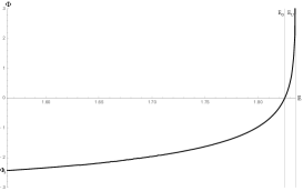
Figure 10: The behaviour of the precession angle $\phi$ as a function of the energy $E$, with $M=1$, $\ell=10$, $Q=1.2$, and $L=6$. Note that the precession angle vanishes when $E=1.825$, it tends to infinity when $E\rightarrow E_{U}\approx 1.836$, and $\Phi\rightarrow\Phi_{S}\approx-2.428$ when the energy $E\rightarrow E_{S}\approx 1.563$.

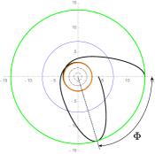
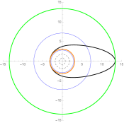
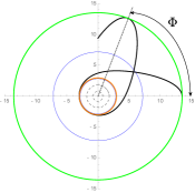
Figure 11: The behaviour of the planetary orbits with $M=1$, $\ell=10$, $Q=1.2$, and $L=6$. Top panel corresponds to an orbit with negative precession $E=1.835$, central panel without precession with $E=1.825$, and bottom panel for a positive precession with $E=1.833$. The green circle represents to the apoastro distance $r_{A}$, the blue circle represents to the stable circular orbit, the orange circle represents to the periastro distance $r_{P}$, the small blue circle represents to the unstable circular orbit $r_{U}$, and the small dashed circle and the dashed circle corresponds to the Cauchy horizon $r_{-}$ and the event horizon $r_{+}$, respectively.

3.2.3 Second kind trajectories

The particles describe second kind trajectories when they start from a point of the spacetime and then they plunge into the horizon. In Fig. 12 we show such trajectories with vanishing and non vanishing precession. In the top panel, we observe that the analytical extension of the geodesics shows a similar trajectory to the Limaçon of Pascal Villanueva:2013zta .

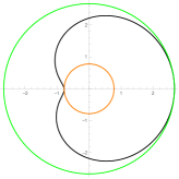
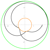
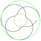
Figure 12: The behaviour of second kind trajectories with $M=1$, $\ell=10$, $Q=1.2$, and $L=6$. Top panel corresponds to an orbit without precession with $E\approx 1.825$, central panel for a positive precession with $E\approx 1.833$, and bottom panel for negative precession $E\approx 1.732$. The orange circle represents a return point ($r_{4}$) inside the Cauchy horizon, and the green circle represents the return point ($r_{F}$) outside the event horizon.

An analytical solution for second kind trajectories described by elementary functions can be found when $E=E_{S}$, and it is given by

$$r_{2K}(\phi)=\sqrt{r_{S}^{2}-\frac{2\left(r_{S}^{2}-r_{4}^{2}\right)\left(r_{S}^{2}-r_{F}^{2}\right)}{\left(-r_{4}^{2}-r_{F}^{2}+2r_{S}^{2}\right)-\left(r_{F}^{2}-r_{4}^{2}\right)\sin\left(\kappa_{2}\phi-\frac{\pi}{2}\right)}}\,,$$ (95)

where $\kappa_{2}=\frac{2}{\ell L}\sqrt{\left(r_{S}^{2}-r_{4}^{2}\right)\left(r_{S}^{2}-r_{F}^{2}\right)}$. In Fig. 13, we plot the above solution and we can see a special second kind trajectory with a negative precession.

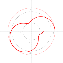
Figure 13: The behaviour of a special second kind trajectories with $M=1$, $\ell=10$, $Q=1.2$, $L=6$, and $E=E_{S}=1.563$. The small circle corresponds to the return point $r_{4}$, the medium circle represent to the event horizon $r_{+}$, and the bigger circle represents the return point $r_{F}$.

3.2.4 Critical trajectories.

This kind of motion is indeed ramified into two cases; critical trajectories of the first kind (CFK) and those of the second kind (CSK) where the particles start from an initial point $d_{i}$ at the vicinity of $r_{i}$ and then tend to this radius by spiraling. We obtain the following equations of motion for the aforementioned trajectories:

$$r_{CFK}(\phi)=\sqrt{r_{u}^{2}-\frac{2\left(r_{u}^{2}-d_{0}^{2}\right)\left(R_{0}^{2}-r_{u}^{2}\right)}{\left(d_{0}^{2}+R_{0}^{2}-2r_{u}^{2}\right)-\left(R_{0}^{2}-d_{0}^{2}\right)\cosh(\kappa_{c}\phi)}}\,,$$ (96)

$$r_{CSK}(\phi)=\sqrt{r_{u}^{2}-\frac{2\left(r_{u}^{2}-d_{0}^{2}\right)\left(R_{0}^{2}-r_{u}^{2}\right)}{\left(R_{0}^{2}-d_{0}^{2}\right)\cosh(k_{c}\phi)+\left(d_{0}^{2}+R_{0}^{2}-2r_{u}^{2}\right)}}\,,$$ (97)

where $\kappa_{c}=\frac{2\sqrt{\left(r_{u}^{2}-d_{0}^{2}\right)\left(R_{0}^{2}-r_{u}^{2}\right)}}{\ell L}$, $R_{0}$ is $\left.r_{A}\right|_{E_{U}}$, and $d_{0}$ is $\left.r_{4}\right|_{E_{U}}$. In Fig. 14, we show the behaviour of the CFK (blue line) and CSK (purple line) trajectories, given by Eq. (96) and Eq. (97).

Figure 14: The behaviour of critical trajectories with $M=1$, $\ell=10$, $Q=1.2$, and $L=6$. Blue line for CFK and purple line for CSK trajectories with $E=E_{U}=1.836$, and $r_{u}=2.861$. The small circle represents to the return point $d_{0}$ inside the Cauchy horizon, the medium circle represents to $r_{u}$, and the bigger circle represents to $R_{0}$.

3.2.5 Motion with $L=0$

As mentioned, for the motion of particles with $L=0$ the effective potential is $V^{2}=f(r)$. Consequently, the equations governing this kind of motion are (53) and (54). Thus, by assuming that particles are placed at $r=r_{0}$ when $t=\tau=0$, so, the turning point $r_{0}$ is located at

$$r_{0}=\sqrt{Z_{0}\cos\Theta_{0}-\ell^{2}(1-E^{2})/3}\,,$$ (98)

where $Z_{0}=2\sqrt{\alpha_{0}/3}$ and $\Theta_{0}=\frac{1}{3}\arccos\left(-\frac{3\sqrt{3}\beta_{0}}{2\alpha_{0}^{3/2}}\right)$, with

$$\alpha_{0}={\ell^{4}(1-E^{2})^{2}\over 3}+4\,M^{2}\,\ell^{2}\,,$$ (99)

$$\beta_{0}={2\,\ell^{6}(1-E^{2})^{3}\over 27}+{4\,M^{2}\,\ell^{4}(1-E^{2})\over 3}+Q^{4}\,\ell^{2}\,.$$ (100)

Therefore, by replacing Eq. (53) into Eq. (54), we obtain the proper time ($\tau$) for the motion of massive particles with $L=0$ in terms of the radial coordinate ($r$), resulting

$$\tau\left(r\right)={r_{0}^{3}\over 8\,Q^{2}}\left[F_{0}(r)-F_{0}(r_{0})\right]\,,$$ (101)

and the coordinate time ($t$) as function of $r$ yields

$$t\left(r\right)=A_{0}\,\sum_{i=1}^{3}A_{i}\,\left[F_{i}(r)-F_{i}(r_{0})\right]\,,$$ (102)

where the functions $F_{j}(r)$ ($j=0,1,2,3$) are given explicitly by

$$F_{j}(r)={\zeta\left(\Omega_{j}\right)\wp^{-1}\left[U(r)\right]+\ln\left|\frac{\sigma\left[\wp^{-1}\left[U(r)\right]-\Omega_{j}\right]}{\sigma\left[\wp^{-1}\left[U(r)\right]+\Omega_{j}\right]}\right|\over\wp^{\,\prime}\left(\Omega_{j}\right)}\,,$$ (103)

$$U(r)={M^{2}\,r_{0}^{2}\over 3Q^{4}}-{r_{0}^{2}\over 4r^{2}}\,,$$ (104)

where the invariants are given by

$$g_{2}={4M^{4}r_{0}^{4}\over 3\,Q^{8}}-{(1-E^{2})r_{0}^{4}\over 4\,Q^{4}}\,,$$ (105)

$$g_{3}={M^{2}(1-E^{2})r_{0}^{6}\over 12\,Q^{8}}-{8M^{6}r_{0}^{6}\over 27\,Q^{12}}+{r_{0}^{6}\over 16\,Q^{4}\,\ell^{2}}\,.$$ (106)

and

$$\Omega_{0}=\wp^{-1}\left({M^{2}r_{0}^{2}\over 3Q^{4}}\right)\,,\,\,\Omega_{1}=\wp^{-1}\left({M^{2}r_{0}^{2}\over 3Q^{4}}-{r_{0}^{2}\over 4\,r^{2}_{+}}\right)\,,$$ (107)

$$\Omega_{2}=\wp^{-1}\left({M^{2}r_{0}^{2}\over 3Q^{4}}-{r_{0}^{2}\over 4\,r^{2}_{-}}\right)\,,\,\,\Omega_{3}=\wp^{-1}\left({M^{2}r_{0}^{2}\over 3Q^{4}}+{r_{0}^{2}\over 4\,r^{2}_{3}}\right)\,,$$ (108)

with the corresponding constants

$$A_{0}={E\ell^{2}r_{0}^{7}\over 8Q^{2}r_{+}^{2}r_{-}^{2}r_{3}^{2}}\,,\,\,A_{1}={r_{+}^{4}r_{-}^{2}r_{3}^{2}\over r_{0}^{4}(r_{+}^{2}-r_{-}^{2})(r_{+}^{2}+r_{3}^{2})}\,,$$ (109)

$$A_{2}=-{r_{+}^{2}r_{-}^{4}r_{3}^{2}\over r_{0}^{4}(r_{+}^{2}-r_{-}^{2})(r_{-}^{2}+r_{3}^{2})}\,,$$ (110)

$$A_{3}=-{r_{+}^{2}r_{-}^{2}r_{3}^{4}\over r_{0}^{4}(r_{-}^{2}+r_{3}^{2})(r_{+}^{2}+r_{3}^{2})}\,,$$ (111)

where $r_{3}\equiv|\sqrt{x_{2}-\ell^{2}/3}|$. Now, in order to visualize the behaviour of the proper and coordinate time, we plot in Fig 15, their behaviour via the solution (101), and (102), respectively. We can observe that the particles cross the event horizon in a finite proper time, but an external observer will see that the particles take an infinite (coordinate) time to do it, the same behaviour was observed for the uncharged background.

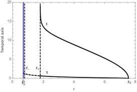
Figure 15: Proper and coordinate time for the motion of test particles with $L=0$. Here we have used the values $E\approx 1.225$, $Q=1.2$, $M=1$, $\ell=10$, and $r_{0}\approx 7.547$. Blue line corresponds to the return point ($\bar{\rho}_{0}=0.699$) inside the Cauchy horizon ($r_{-}\approx 0.783$), the dashed line corresponds to the Cauchy and event horizon ($r_{+}\approx 1.805$).

4 Final remarks

Through this work we have considered the motion of neutral particles in the background of five-dimensional Schwarzschild Anti de Sitter (SAdS) and Reissner Nordström Anti de Sitter (RNAdS) black holes, and we established the time-like structure geodesic in order to complete the geodesics structure of this spacetime, and also to study the effect of the black hole charge in the geodesics. As we have seen, the time-like geodesics structure have been determined analytically and also the geodesics have been plotted in order to see their behaviour.

Concerning to the horizons, the five-dimensional SAdS black hole present only the event horizon, while that RNAdS black hole present the event horizon and the Cauchy horizon. At the level of the effective potential, the trajectories are qualitatively similar for fixed values of the mass, cosmological constant, angular momentum and energy. However, for the charged case there is a return point located at $r<r_{-}$, which implies that the trajectory do not reach the singularity $r=0$. Specifically, for the circular orbits, we have shown that the effect of the charge is to increase the energy necessary in order to obtain an unstable circular orbit, but the radius of such orbit decreases. With respect to the stable circular orbit, the effect of the charge is to increase the energy necessary in order to obtain the stable circular orbit, but the radius of such orbit increases. Also, the effect of the black hole charge is to increase the affine and coordinate period. For the planetary orbits, the effect of the black hole charge is to increase the periastro distance and to decrease the apoastro distance. Also, both spacetimes allow planetary orbits with negative, null and positive precession. But, the black hole charge increases the energy value for a null precession. For the other relativistic orbits, as second kind and critical trajectories, the black hole charge implies the existence of a return point between the singularity and the Cauchy horizon. For the motion with $L=0$ in the Schwarzschild AdS black hole the particles cross the event horizon in a finite proper time and reach the singularity, but for an external observer the particles take an infinite coordinate time to reach the event horizon. However, the difference for charged spacetime is that particles that cross the event horizon in finite proper time cannot reach the singularity.

Could be interesting to consider the motion of charged particles in order to analyze the influence of the charge of the particles on the orbits, we hope to address it, in a forthcoming work.

Acknowlegements

This work is partially supported by ANID Chile through FONDECYT Grant Nº 1220871 (P.A.G., and Y. V.). J.R.V. was partially supported by Centro de Astrofísica de Valparaíso.

References

- (1) T. Kaluza, “Zum Unitätsproblem der Physik,” Sitzungsber. Königl. Preuss. Akad. Wiss.”, pp. 966-972, 1921.
- (2) O. Klein, “Quantentheorie und fünfdimensionale relativitätstheorie”, Zeitschrift für Physik, 1926.
- (3) A. Font and S. Theisen, “Introduction to string compactification,” Lect. Notes Phys. 668 (2005) 101.
- (4) C. S. Chan, P. L. Paul and H. L. Verlinde, “A Note on warped string compactification,” Nucl. Phys. B 581 (2000) 156 [hep-th/0003236].
- (5) F. R. Tangherlini, “Schwarzschild field in n dimensions and the dimensionality of space problem,” Nuovo Cim. 27, 636 (1963).
- (6) J. M. Maldacena, “The Large N limit of superconformal field theories and supergravity,” Int. J. Theor. Phys. 38 (1999) 1113 [Adv. Theor. Math. Phys. 2 (1998) 231] [hep-th/9711200].
- (7) E. Witten, “Anti-de Sitter space and holography,” Adv. Theor. Math. Phys. 2 (1998) 253 [hep-th/9802150].
- (8) S. S. Gubser, I. R. Klebanov and A. M. Polyakov, “Gauge theory correlators from noncritical string theory,” Phys. Lett. B 428 (1998) 105 [hep-th/9802109].
- (9) J. J. Friess, S. S. Gubser, G. Michalogiorgakis and S. S. Pufu, “Expanding plasmas and quasinormal modes of anti-de Sitter black holes,” JHEP 0704 (2007) 080 [hep-th/0611005].
- (10) J. R. Villanueva, J. Saavedra, M. Olivares and N. Cruz, “Photons motion in charged Anti-de Sitter black holes,” Astrophys. Space Sci. 344 (2013) 437.
- (11) P. A. González, M. Olivares, Y. Vásquez and J. R. Villanueva, “Null geodesics in five-dimensional Reissner-Nordstrm anti-de Sitter black hole,” Eur. Phys. J. C 81 (2021) no.3, 236 [arXiv:2010.01442 [gr-qc]].
- (12) H. Saadat, “Thermodynamics and stability of five dimensional AdS Reissner-Nordstroem black hole,” Int. J. Theor. Phys. 51 (2012) 316.
- (13) A. Chamblin, R. Emparan, C. V. Johnson and R. C. Myers, “Charged AdS black holes and catastrophic holography,” Phys. Rev. D 60 (1999) 064018 [hep-th/9902170].
- (14) A. Chamblin, R. Emparan, C. V. Johnson and R. C. Myers, “Holography, thermodynamics and fluctuations of charged AdS black holes,” Phys. Rev. D 60 (1999) 104026 [hep-th/9904197].
- (15) Page, Don N. and Kubizňák, David and Vasudevan, Muraari and Krtouš, Pavel, “Complete Integrability of Geodesic Motion in General Higher-Dimensional Rotating Black-Hole Spacetimes,” Phys. Rev. Lett. 98 (2007)
- (16) V. P. Frolov and D. Stojkovic, “Particle and light motion in a space-time of a five-dimensional rotating black hole,” Phys. Rev. D 68, 064011 (2003) [gr-qc/0301016].
- (17) E. Hackmann, V. Kagramanova, J. Kunz and C. Lammerzahl, “Analytic solutions of the geodesic equation in higher dimensional static spherically symmetric space-times,” Phys. Rev. D 78 (2008) 124018 Addendum: [Phys. Rev. D 79 (2009) no.2, 029901] [arXiv:0812.2428 [gr-qc]].
- (18) G. W. Gibbons and M. Vyska, “The Application of Weierstrass elliptic functions to Schwarzschild Null Geodesics,” Class. Quant. Grav. 29 (2012) 065016 [arXiv:1110.6508 [gr-qc]].
- (19) S. Guha, S. Chakraborty and P. Bhattacharya, “Particle motion in the field of a five-dimensional charged black hole,” Astrophys. Space Sci. 341 (2012), 445-455 [arXiv:1008.2650 [gr-qc]].
- (20) D. Kovacs, “The Geodesic Equation In Five-dimensional Relativity Theory Of Kaluza-klein,” Gen. Rel. Grav. 16 (1984) 645.
- (21) V. Kagramanova and S. Reimers, “Analytic treatment of geodesics in five-dimensional Myers-Perry space–times,” Phys. Rev. D 86 (2012) 084029 [arXiv:1208.3686 [gr-qc]].
- (22) S. S. Seahra and P. S. Wesson, “Null geodesics in five-dimensional manifolds,” Gen. Rel. Grav. 33 (2001) 1731 [gr-qc/0105041].
- (23) S. Guha and P. Bhattacharya, “Geodesic motions near a five-dimensional Reissner-Nordstroem anti-de Sitter black hole,” J. Phys. Conf. Ser. 405 (2012) 012017.
- (24) P. A. Gonzalez, M. Olivares and Y. Vasquez, “Bounded orbits for photons as a consequence of extra dimensions,” Mod. Phys. Lett. A 32 (2017) no.32, 1750173 [arXiv:1511.08048 [gr-qc]].
- (25) S. Grunau, H. Neumann and S. Reimers, “Geodesic motion in the five-dimensional Myers-Perry-AdS spacetime,” Phys. Rev. D 97 (2018) no.4, 044011 [arXiv:1711.02933 [gr-qc]].
- (26) J. Chandler and M. H. Emam, “Geodesic structure of five-dimensional nonasymptotically flat 2-branes,” Phys. Rev. D 91, no. 12, 125024 (2015) [arXiv:1506.06054 [gr-qc]].
- (27) R. S. Kuniyal, H. Nandan, U. Papnoi, R. Uniyal and K. D. Purohit, “Strong lensing and observables around 5D Myers–Perry black hole spacetime,” Mod. Phys. Lett. A 33 (2018) no.23, 1850126 [arXiv:1705.09232 [gr-qc]].
- (28) T. V. Fernandes and J. P. S. Lemos, “Electrically charged spherical matter shells in higher dimensions: Entropy, thermodynamic stability, and the black hole limit,” Phys. Rev. D 106 (2022), 104008
- (29) R. André and J. P. S. Lemos, “Thermodynamics of d-dimensional Schwarzschild black holes in the canonical ensemble,” Phys. Rev. D 103 (2021), 064069
- (30) X.Kong, T. Wang, L. Zhao, “High temperature AdS black holes are low temperature quantum phonon gases,” Phys. Lett. B 836 (2023) 137623
- (31) S. Mandal, S. Upadhyay, Y. Myrzakulov and G. Yergaliyeva, “Shadow of the 5D Reissner–Nordström AdS black hole,” Int. J. Mod. Phys. A 38 (2023) no.08, 2350047 [arXiv:2207.10085 [gr-qc]].
- (32) S. Chandrasekhar, “The mathematical theory of black holes”, Oxford University Press, 2002.
- (33) N. Cruz, M. Olivares and J. R. Villanueva, “The Geodesic structure of the Schwarzschild anti-de Sitter black hole,” Class. Quant. Grav. 22 (2005) 1167 [gr-qc/0408016].
- (34) J. R. Villanueva, F. Tapia, M. Molina and M. Olivares, “Null paths on a toroidal topological black hole in conformal Weyl gravity,” Eur. Phys. J. C 78 (2018) no.10, 853 [arXiv:1808.04298 [gr-qc]].
- (35) J. Ramos-Caro, J. F. Pedraza and P. S. Letelier, “Motion around a Monopole + Ring system: I. Stability of Equatorial Circular Orbits vs Regularity of Three-dimensional Motion,” Mon. Not. Roy. Astron. Soc. 414, 3105 (2011) [arXiv:1103.4616 [astro-ph.EP]].