Lie-algebraic classical simulations for variational quantum computing

Abstract

Classical simulation of quantum dynamics plays an important role in our understanding of quantum complexity, and in the development of quantum technologies. Compared to other techniques for efficient classical simulations, methods relying on the Lie-algebraic structure of quantum dynamics have received relatively little attention. At their core, these simulations leverage the underlying Lie algebra – and the associated Lie group – of a dynamical process. As such, rather than keeping track of the individual entries of large matrices, one instead keeps track of how its algebraic decomposition changes during the evolution. When the dimension of the algebra is small (e.g., growing at most polynomially in the system size), one can leverage efficient simulation techniques. In this work, we review the basis for such methods, presenting a framework that we call ‘$\mathfrak{g}{\text{-}}{\rm sim}$’, and showcase their efficient implementation in several paradigmatic variational quantum computing tasks. Specifically, we perform Lie-algebraic simulations to train and optimize parametrized quantum circuits, design enhanced parameter initialization strategies, solve tasks of quantum circuit synthesis, and train a quantum-phase classifier.

I Introduction

At a fundamental level, the ability to classically simulate quantum dynamics in certain regimes helps us to refine our understanding of the true nature of quantum complexity. Different approaches allowing for scalable classical simulations have elucidated distinct aspects of quantumness by restricting the set of operations performed, the initial states evolved, and the observables measured. These include, but are not limited to, the role of the discrete-group structure of Clifford operations in the case of stabilizer simulations [1], the importance of entanglement in the case of tensor networks [2], and the existence of transformations to non-interacting particles in the case of free fermions [3, 4]. For all the these approaches, the computational resources required for simulations scale only polynomially in the system size, as opposed to the exponential cost of the generic or unrestricted case. Such simulations are deemed classically efficient or scalable.

At a practical level, the ability to efficiently simulate quantum systems facilitates the development of quantum technology. As the size of experimentally demonstrated quantum systems is starting to exceed what can be simulated classically, it is of great importance to rely on faithful classical computational results [5]. In this context, classical simulations can serve the role of benchmarks for currently developed devices and can be used for the purpose of characterization. Furthermore, classical simulations can find many more applications along the development and study of variational quantum computing. These encompass variational quantum algorithms (VQAs) [6, 7] and quantum machine learning (QML) methods [8, 9, 10, 11], that most typically rely on the ability to optimize over parameters of quantum circuits. Despite the promises of such algorithms and demonstrations for relatively small system sizes, it remains unclear how viable these are when scaled to larger sizes [12, 13, 14]. As such, scalable quantum simulators can serve to improve VQAs and QML models. For instance, classical simulations can be used to provide exact inputs for learning-based error mitigation strategies [15, 16, 17, 18], to probe the trainability of quantum circuits at large scale [19], and for the purpose of pre-training the models [20, 21, 22, 23, 24, 25, 26, 27, 28, 29, 30].

Among the scalable simulation methods that have been proposed, we focus on those based on the Lie-algebraic structure of the underlying dynamics [31, 32, 33]. Here, simulation complexity scales with the dimension (denoted $\operatorname{dim}(\mathfrak{g})$) of the Lie-algebra (denoted $\mathfrak{g}$) induced by the operators generating the dynamics of the system - these notions are defined more precisely soon. Crucially, in certain cases such dimension can be substantially smaller that the dimension of the Hilbert space of the system of interest, allowing for more efficient simulations that would be entailed generically. In particular, such simulations become scalable whenever $\operatorname{dim}(\mathfrak{g})$ grows polynomially with the system size $n$ (i.e., $\operatorname{dim}(\mathfrak{g})\in\mathcal{O}(\operatorname{poly}(n))$). For example, this is known to occur in systems with underlying free-fermionic algebras [34, 35] or with permutation symmetries [36, 33].

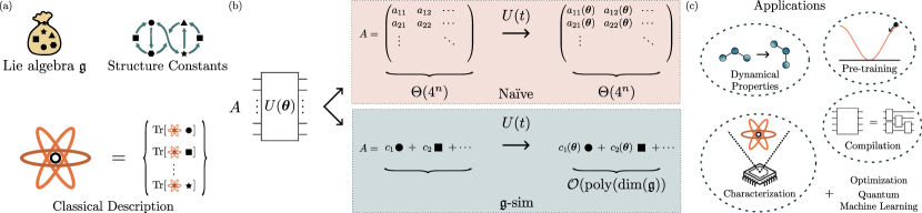
Figure 1: Theoretical framework and applications of $\mathfrak{g}$-sim. (a) Essential components of the Lie-algebraic representation of quantum dynamics. First, we need a description of the Lie algebra $\mathfrak{g}$ associated with a unitary evolution of interest. Here we depict the elements of $\mathfrak{g}$ as a collection of black geometric shapes. Next, we need to know how these elements inter-connect to each other via the dynamics. This is determined entirely by the so-called structure constants. The final ingredient of $\mathfrak{g}{\text{-}}{\rm sim}$ is a classical description of the input state, i.e., the expectation values with respect to the elements of $\mathfrak{g}$. (b) Comparison of naïve and Lie-algebraic approaches to quantum dynamics in the Heisenberg picture. In the naïve approach, an observable $A$ is viewed as a linear operator acting on an $n$-qubit Hilbert space $\mathcal{H}$, with $\operatorname{dim}(\mathcal{H})=2^{n}$. The observable is represented as a $2^{n}\times 2^{n}$ matrix whose coefficients evolve according to the von Neumann equation of motion, and thus the approach always scales as $\Theta(4^{n})$ and is not classically scalable. In the Lie-algebraic approach, the observable is instead viewed as a linear combination of distinct basis terms in $\mathfrak{g}$, whose coefficients couple to each other over time via the structure constants. Whenever $\operatorname{dim}(\mathfrak{g})\in\mathcal{O}(\operatorname{poly}(n))$, $\mathfrak{g}{\text{-}}{\rm sim}$ yields a scalable classical simulation framework. (c) Summary of the potential applications of $\mathfrak{g}{\text{-}}{\rm sim}$. These efficient classical simulations have utility in simulation and optimization of quantum systems, including pre-training of VQA or QML problems, compiling unitary processes to compact quantum circuits, and characterizing QML optimization landscapes.

In this work, we provide guidelines for the efficient implementation of Lie-algebraic simulations (referred to as $\mathfrak{g}{\text{-}}{\rm sim}$). We highlight the fact that these simulation techniques are well known [31, 32], so our first contribution is to present them in a modern language oriented to the quantum computing community, offer new optimizations that improve their efficiency, and extend their utility to optimizing circuits (as opposed to merely simulating them). Our second, and main, contribution is to showcase the utility of $\mathfrak{g}{\text{-}}{\rm sim}$ in four different tasks pertaining to the development of quantum technologies. These include the study of the optimization landscapes of parametrized quantum circuits, improving on the initializations of such circuits, problems of quantum circuit synthesis, and the training of a binary quantum-phase classifier. In particular, our implementation of $\mathfrak{g}{\text{-}}{\rm sim}$ for circuit synthesis is novel as the techniques of Refs. [31, 32] have not previously been extended to quantum compilation. A high-level overview of our theoretical framework and applications for this work is provided in Fig. 1.

In the first part of this work (Sec. II) we review the theory grounding Lie-algebraic simulations and provide guidelines for their efficient implementations. The exposition here is aimed to be pedagogical, with an eye towards generic and efficient algorithms. It follows from Refs. [31, 32], and extends them in terms of scope and implementation (including both the ability to simulate and differentiate evolution).

In the second part (Sec. III), $\mathfrak{g}{\text{-}}{\rm sim}$ is put into practice in four distinct scenarios. As a warm-up example, we provide a large scale study of the overparametrization phenomenon (Sec. III.1). Then, $\mathfrak{g}{\text{-}}{\rm sim}$ is applied for the purpose of the initialization of (non-classically-simulable) circuits in two different setups (Sec. III.2). Next, tasks of circuit synthesis and dynamical evolution are addressed (Sec. III.3). Finally, as an application in the context of QML, we resort to $\mathfrak{g}{\text{-}}{\rm sim}$ to train a quantum-phase classifier (Sec. III.4). Overall, these examples aim at illustrating the diversity of tasks that can be accomplished via $\mathfrak{g}{\text{-}}{\rm sim}$, and also showcase some avoidable pitfalls.

II Framework

II.1 Set-up

Thorough this article we focus on quantum dynamics realized by means of quantum circuits (i.e., digital quantum computations), but stress that the same principles can equally be applied to continuously driven systems (i.e., analog quantum computations). Also, we restrict the main discussions to unitary dynamics, however this can be generalized to mixed-unitary channels. Both these aspects are detailed further in Appendix A. Finally, we note that while exposed in the context of the qubit model, the same principles are readily ported to other models of quantum physics.

With this scope in mind, we will henceforth study a system of $n$ qubits with an associated Hilbert space $\mathcal{H}=(\mathbb{C}^{2})^{\otimes n}$ of dimension $d=2^{n}$. We further consider the case when the dynamics of the quantum system are determined by a unitary operator

$$U(\bm{\theta})=\prod_{l=1}^{L}\prod_{k=1}^{K}e^{-i\theta_{lk}H_{k}}\,,$$ (1)

specified in terms of variable angles (or parameters) $\bm{\theta}=[\theta_{11},\ldots,\theta_{LK}]$ and of a finite set of $K$ Hermitian operators $\{H_{1},\dots,H_{K}\}$ which are the gate generators of the circuit. This structure is repeated over $L$ layers. We note that Eq. (1) accounts for ansätze with periodic structure and layered structure, but also for unitaries with non-periodic structure (by setting $L=1$), as well as for unitaries with fixed gates (by fixing some of the parameters $\theta_{lk}$).

In the following we will be concerned with tasks of simulation and optimization of quantum circuits. For an observable $O$, an initial state $\rho^{(\operatorname{in})}$, and a circuit $U(\bm{\theta})$, simulation consists of evaluating the expectation value of $O$ for the evolved state $\rho^{(\operatorname{out})}(\bm{\theta})\equiv U(\bm{\theta})\rho^{(\operatorname{in})}U^{\dagger}(\bm{\theta})$. That is, by simulation we mean the evaluation of a quantity of the form

$$\langle O(\bm{\theta})\rangle\equiv\Tr[OU(\bm{\theta})\rho^{(\operatorname{in})}U^{\dagger}(\bm{\theta})]=\Tr[O\rho^{(\operatorname{out})}(\bm{\theta})]\,.$$ (2)

In addition to simulation, one is often interested in actively optimizing the system’s dynamics to achieve a certain objective. For instance, this is at the core of most problems found in the field of VQAs and QML. These rely on optimizing circuit parameters to decrease the value of a loss function that can be evaluated through expectation values. As an example, in a variational quantum eigensolver (VQE) [37] aiming at preparing the ground state of an Hamiltonian $H$, this loss would be the expectation value $\langle H(\bm{\theta})\rangle$. Similarly, in the context of QML, the same circuit unitary may be applied to a dataset of quantum states, and the loss to be minimized could be a function of expectation values of a set of observables $\{O_{i}\}$ that are obtained for each state. In both cases, optimization of the circuit parameters can be enhanced by the ability to compute gradients of the form $\partial_{\bm{\theta}}\langle O(\bm{\theta})\rangle$.

II.2 Lie theory

Here we recall elementary results of Lie theory that are relevant to this work. For a general treatment of Lie groups and Lie algebras, we recommend standard textbooks  [38, 39]. A more specific presentation of Lie theory in the context of quantum control can be found in Refs. [40, 41], or in the context of quantum circuits in Refs. [42, 43]. We start by reviewing the concepts of dynamical Lie algebra (Definition 1) and dynamical Lie group (Definition 2) which characterize the expressiveness of quantum circuits of the form in Eq. (1).

Definition 1 (Dynamical Lie algebra).

Consider an ansatz of the form in Eq. (1). Its dynamical Lie algebra $\mathfrak{g}$ is defined as the vector space spanned by all the possible nested commutators of $\{iH_{1},\dots,iH_{K}\}$. That is,

$$\mathfrak{g}={\rm span}_{\mathbb{R}}\left\langle\{iH_{1},\ldots,iH_{K}\}\right\rangle_{\operatorname{Lie}}\subseteq\mathfrak{su}(2^{n})\,,$$ (3)

where $\left\langle S\right\rangle_{\operatorname{Lie}}$ denotes the Lie closure of S, i.e., the set of elements obtained by repeatedly taking the commutator between elements in $S$ until no new linearly independent elements are obtained. We denote as $G_{\alpha}$ (with $\alpha=1,\ldots,\operatorname{dim}(\mathfrak{g})$) the Hermitian operators such that $\{iG_{\alpha}\}_{\alpha}$ forms a Schmidt-orthonormal basis of $\mathfrak{g}$.

The dynamical Lie algebra $\mathfrak{g}$ constitutes a Lie subalgebra of the special unitary Lie algebra $\mathfrak{su}(2^{n})$, the space of linear anti-Hermitian operators acting on the $n$-qubit system. Often, we will say that an observable $A$ is supported by the algebra whenever $iA\in\mathfrak{g}$, i.e., whenever $A$ can be expanded in the basis of observables $\{G_{\alpha}\}_{\alpha}$. For details on numerical algorithms to compute the Lie closure we refer to Refs. [41, 42].

In correspondence to the dynamical Lie algebra $\mathfrak{g}$, we can also define the dynamical Lie group $\mathcal{G}$ as follows.

Definition 2 (Dynamical Lie group).

The dynamical Lie group $\mathcal{G}$ of a circuit of the form Eq. (1) is determined by its dynamical Lie algebra $\mathfrak{g}$ and defined as

$$\mathcal{G}=e^{\mathfrak{g}}\equiv\{e^{iA},\quad iA\in\mathfrak{g}\}\,.$$ (4)

Notably, the dynamical Lie group $\mathcal{G}$ corresponds to all possible unitaries that can be implemented by circuits of the form in Eq. (1). That is, for every $V\in\mathcal{G}$ there exists (at least) one choice of parameter values $\bm{\theta}$ for a sufficiently large, but finite, number of layers $L$ such that $U(\bm{\theta})=V$ [40]. Overall, $\mathfrak{g}$ determines the group $\mathcal{G}$ of unitaries that could be realized, and we can take their dimensions in correspondence: ${\rm dim}(\mathcal{G})\text{ (as a smooth differentiable manifold)}=\operatorname{dim}(\mathfrak{g})$.

Having characterized the Lie algebra and group associated with the dynamical process in Eq. (1), we need to study how their elements act. That is, how the elements of the algebra transform under commutation with elements of $\mathfrak{g}$, and under conjugation with elements of $\mathcal{G}$.

We begin by recalling that since a (matrix) Lie algebra $\mathfrak{g}$ is closed under commutation, it is fully characterized by its structure constants $f^{\gamma}_{\alpha\beta}=\Tr[iG_{\gamma}\left[iG_{\alpha},iG_{\beta}\right]]\in\mathbb{R}$, through

$$[iG_{\alpha},iG_{\beta}]=\sum_{\gamma=1}^{\operatorname{dim}(\mathfrak{g})}f^{\gamma}_{\alpha\beta}iG_{\gamma}\,.$$ (5)

More importantly, these constants provide a way to describe the action of the Lie algebra over the $2^{n}\times 2^{n}$ operators in the basis of $\mathfrak{g}$ in terms of $\operatorname{dim}(\mathfrak{g})\times\operatorname{dim}(\mathfrak{g})$ matrices. Specifically, we leverage the following definition.

Definition 3 (adjoint representation of $\mathfrak{g}$).

Given an operator $iG_{l}$ in the basis of $\mathfrak{g}$, its adjoint representation is obtained via the map $\Phi_{\mathfrak{g}}^{\operatorname{ad}}:\mathfrak{g}\mapsto\mathbb{R}^{\operatorname{dim}(\mathfrak{g})\times\operatorname{dim}(\mathfrak{g})}$ and is defined by

$$\left(\Phi_{\mathfrak{g}}^{\operatorname{ad}}(iG_{\gamma})\right)_{\alpha\beta}\equiv f_{\alpha\beta}^{\gamma}=\Tr[iG_{\gamma}\left[iG_{\alpha},iG_{\beta}\right]]\,.$$ (6)

We note that if the underlying algebra is compact, and if the basis observables $G_{\alpha}$ are Schmidt-orthonormal the adjoint representation is faithful [31] (i.e. the map $\Phi_{\mathfrak{g}}$ is injective). It is clear that because of the linearity of the adjoint representation, Definition 6 implies that knowledge of the adjoint representations of the $\operatorname{dim}(\mathfrak{g})$ basis observables is sufficient to obtain the representations of any element of $\mathfrak{g}$. That is, for any $A=\sum_{\alpha}(\bm{w})_{\alpha}G_{\alpha}$ (with $\bm{w}\in\mathbb{R}^{\operatorname{dim}(\mathfrak{g})}$) supported by the algebra, one has $\Phi_{\mathfrak{g}}^{\operatorname{ad}}(A)=\sum_{\alpha}(\bm{w})_{\alpha}\Phi_{\mathfrak{g}}^{\operatorname{ad}}(G_{\alpha})$.

Next, by means of the exponential map, we can obtain the adjoint representation of the elements of the Lie group $\mathcal{G}$.

Definition 4 (Adjoint representation of $\mathcal{G}$).

The adjoint representation of $\mathfrak{g}$ induces the adjoint representation $\Phi_{\mathcal{G}}^{\operatorname{Ad}}$ of $\mathcal{G}$. This representation is a linear map $\Phi_{\mathcal{G}}^{\operatorname{Ad}}:\mathcal{G}\mapsto\mathbb{GL}(\mathbb{R}^{\operatorname{dim}(\mathfrak{g})})\subset\mathbb{R}^{\operatorname{dim}(\mathfrak{g})\times\operatorname{dim}(\mathfrak{g})}$ from the group $\mathcal{G}$ to the group of invertible linear operators $\mathbb{GL}(\mathbb{R}^{\operatorname{dim}(\mathfrak{g})})$, defined as

$$\Phi^{Ad}_{\mathcal{G}}(U=e^{iA})=e^{i\bar{\bm{A}}}\,,$$ (7)

for all $iA\in\mathfrak{g}$ (or any $U\in\mathcal{G}$), and with $\bar{\bm{A}}\equiv\Phi_{\mathfrak{g}}^{\operatorname{ad}}(A)$.

For our purposes, the main appeal of such representation is that it exploits the fact that a Lie algebra is closed under the action of its associated Lie group, and hence it allows us to evaluate the action of any $U\in\mathcal{G}$ over any basis observable $G_{\alpha}$ as

$$U^{\dagger}G_{\alpha}U=\sum_{\alpha}\left(\Phi^{\operatorname{Ad}}_{\mathcal{G}}(U)\right)_{\alpha\beta}G_{\beta}\,.$$ (8)

We refer the reader to Ref. [31] or to Appendix A.1 for more details on Eq. (8). As further detailed below, these adjoint representations allow us to perform (Heisenberg) evolution of any operator in the algebra under the action of any $U\in\mathcal{G}$ with a time complexity scaling with $\mathcal{O}(\operatorname{poly}(\operatorname{dim}(\mathfrak{g})))$ as opposed to $\Theta(4^{n})$.

Before moving further, we highlight that faithfulness of a Lie algebra representation does not imply faithfulness of its corresponding Lie group representation. To understand this, we need to recall what the center $Z(\mathcal{G})$ of $\mathcal{G}$ is.

Definition 5 (Center of a group).

The center of a group $\mathcal{G}$ is the subset of $\mathcal{G}$ that simultaneously commute with all elements of $\mathcal{G}$. That is,

$$Z(\mathcal{G})\equiv\{W\in\mathcal{G}\mid\forall U\in\mathcal{G},WU=UW\}\,.$$ (9)

Specifically, one can readily verify that for any $U=e^{iA}$ and $W\in Z(\mathcal{G})$, we have

$$\Phi^{\operatorname{Ad}}_{\mathcal{G}}(WU)=\Phi^{\operatorname{Ad}}_{\mathcal{G}}(UW)=\Phi^{\operatorname{Ad}}_{\mathcal{G}}(U)\,,$$ (10)

showing that a non-trivial center $Z(\mathcal{G})$ results in unfaithfulness of $\Phi^{\operatorname{Ad}}_{\mathcal{G}}$. Even though the Lie algebras $\mathfrak{g}$ considered in this work are centerless, the Lie groups $\mathcal{G}=e^{\mathfrak{g}}$ can still have a nontrivial center, leading to unfaithfulness of $\Phi_{\mathcal{G}}^{\operatorname{Ad}}$. While not an issue for most situations encountered, we will see later in Sec. III.3 that this introduces additional considerations for unitary compilation.

II.3 $\mathfrak{g}$-sim principles

In this section we present the main results which comprise the foundation of $\mathfrak{g}{\text{-}}{\rm sim}$ including simulations with observables supported by $\mathfrak{g}$ (Sec. II.3.1), simulations with observables that are products of terms supported by $\mathfrak{g}$ (Sec. II.3.2), and optimizations (Sec. II.3.3).

II.3.1 Simulation with observables supported by $\mathfrak{g}$

We start by considering simulation problems where the observable of interest is supported by the Lie algebra. That is, we want to evaluate Eq. (2) when $O\in i\mathfrak{g}$. Here, we find it convenient to define $\operatorname{dim}(\mathfrak{g})$-dimensional vectors of expectation values that captures the description of the states $\rho^{(\operatorname{in/out})}$ over the basis observables $G_{\alpha}$:

$$\left(\bm{e}^{(\operatorname{in/out})}\right)_{\alpha}\equiv\Tr[G_{\alpha}\rho^{(\operatorname{in/out})}]\,.$$ (11)

The following result holds.

Result 1 (Simulation of observables in the algebra. Rephrased from [31]).

Consider a circuit of the form in Eq. (1), and let $O$ be an observable with support in $i\mathfrak{g}$ such that $O=\sum_{\alpha}(\bm{w})_{\alpha}G_{\alpha}$ for $\bm{w}\in\mathbb{R}^{\operatorname{dim}(\mathfrak{g})}$. Then, given $\bm{e}^{(\operatorname{in})}$, we can compute

$$\langle O(\bm{\theta})\rangle=\bm{w}\cdot\bm{e}^{(\operatorname{out})}\,,$$ (12)

with the vector of output expectation values obtained as

$$\bm{e}^{(\operatorname{out})}=\left(\prod_{l=1}^{L}\prod_{k=1}^{K}e^{-i\theta_{lk}\bar{\bm{H}}_{k}}\right)\cdot\bm{e}^{(\operatorname{in})},$$ (13)

where $\bar{\bm{H}}_{k}\equiv\Phi_{\mathfrak{g}}^{\operatorname{ad}}(H_{k})$.

Result 1 indicates that, in order to compute $\langle O(\bm{\theta})\rangle$, it suffices to have a decomposition of $O$ in the algebra, the adjoint representations $\bar{\bm{H}}_{k}$ of the gate generators, and the vector of expectation values of the basis observables $\{G_{\alpha}\}_{\alpha}$ for the input state. We stress that although Eq. (13) resembles unitary evolution in the Hilbert space $\mathcal{H}$, it differs subtly. The vectors $\bm{e}^{(\operatorname{in/out})}$ are not state vectors in the usual sense, but vectors of expectation values of observables, and consequently the phases (signs) are indeed physical. Since the $\bar{\bm{H}}_{k}$ are purely imaginary Hermitian matrices, the gate representations $e^{-i\theta_{m}\bar{\bm{H}}_{k}}$ are real-valued, and describe linear coupling between observables induced by unitary evolution.

An immediate consequence of Result 1 is that we can compute expectation values of observables supported by the algebra with a time complexity scaling as $\mathcal{O}(LK\operatorname{dim}(\mathfrak{g})^{3})$. However, as detailed in Appendix B.1, we provide a more efficient algorithm based on a full-rank eigendecomposition of the $\bar{\bm{H}}_{k}$ matrices. Further improvements for algebras with a Pauli basis are provided in Appendices B.2 and B.3. This leads us to our first main contribution, which improves on the time complexity of $\mathfrak{g}{\text{-}}{\rm sim}$.

Theorem 1.

Computing expectation values of observables supported by the algebra using $\mathfrak{g}{\text{-}}{\rm sim}$ has a time complexity in $\mathcal{O}(LK\operatorname{dim}(\mathfrak{g})^{2})$ for circuits of the form in Eq. (1).

In Appendix A.2 we also present a theorem that generalizes Result 1 (valid for unitary evolutions) to mixed-unitary quantum channels.

II.3.2 Simulation with products of observables supported by $\mathfrak{g}$

Here, we consider the task of simulating the expectation values of products of observables supported by the Lie algebra, and first focus on simulating correlators of the form $\langle O^{(1)}O^{(2)}(\bm{\theta})\rangle=\Tr[OU(\bm{\theta})\rho^{(\operatorname{in})}U^{\dagger}(\bm{\theta})]$ for $O^{(1)},O^{(2)}\in i\mathfrak{g}$, even when $O^{(1)}O^{(2)}\notin\mathfrak{g}$. For these, we define a $(\operatorname{dim}(\mathfrak{g})\times\operatorname{dim}(\mathfrak{g}))$-dimensional matrix of expectation values that captures the description of the states $\rho^{(\operatorname{in/out})}$ over products of the basis observables

$$(\bm{E}^{(\operatorname{in/out})})_{\alpha\beta}\equiv\Tr[G_{\alpha}G_{\beta}\rho^{(\operatorname{in/out})}]\,.$$ (14)

We have that the following result holds.

Result 2 (Simulation of product of two operators in the algebra. Rephrased from [31]).

Consider a circuit of the form in Eq. (1), and let $O^{(1)}$ and $O^{(2)}$ be observables with support in $i\mathfrak{g}$ such that $O^{(1)}=\sum_{\alpha}(\bm{w}^{(1)})_{\alpha}G_{\alpha}$ and $O^{(2)}=\sum_{\beta}(\bm{w}^{(2)})_{\beta}G_{\beta}$ for $\bm{w}^{(1)},\bm{w}^{(2)}\in\mathbb{R}^{\operatorname{dim}(\mathfrak{g})}$. Then, given $\bm{E}^{(\operatorname{in})}$, we can compute

$$\langle O^{(1)}O^{(2)}(\bm{\theta})\rangle=(\bm{w}^{(1)})^{T}\cdot\bm{E}^{(\operatorname{out})}\cdot\bm{w}^{(2)}\,,$$ (15)

with the superscript $T$ denoting the matrix transpose, and with the matrix of output expectation values obtained as

$$\bm{E}^{(\operatorname{out})}\!\!=\left(\prod_{l=1}^{L}\prod_{k=1}^{K}e^{-i\theta_{lk}\bar{\bm{H}}_{k}}\right)\bm{E}^{(\operatorname{in})}\left(\prod_{l=1}^{L}\prod_{k=1}^{K}e^{-i\theta_{lk}\bar{\bm{H}}_{k}}\right)^{T}\!\!.$$ (16)

In Appendix A.3 we present generalization of Result 16 to mixed-unitary quantum channels.

Combining Results 1 and 16 we can simulate expectation values of observables of the form

$$O=\sum_{\alpha=1}^{\operatorname{dim}(\mathfrak{g})}(\bm{w}^{(1)})_{\alpha}G_{\alpha}+\sum_{\beta,\gamma=1}^{\operatorname{dim}(\mathfrak{g})}(\bm{W}^{(2)})_{\beta\gamma}G_{\beta}G_{\gamma}$$ (17)

for $\bm{w}^{(1)}\in\mathbb{R}^{\operatorname{dim}(\mathfrak{g})}$ and $\bm{W}^{(2)}\in\mathbb{R}^{\operatorname{dim}(\mathfrak{g})\times\operatorname{dim}(\mathfrak{g})}$. At this point it is worth mentioning that evolution of observables (Result 1) involves only matrix-vector multiplication, whilst evolution of correlators (Result 16) is more expensive as it requires matrix-matrix multiplication. This can be made precise in the following Corollary.

Corollary 1.

Computing expectation values of products of observables supported by the algebra using $\mathfrak{g}{\text{-}}{\rm sim}$ has a time complexity in $\mathcal{O}(LK\operatorname{dim}(\mathfrak{g})^{3})$.

Going further, $\mathfrak{g}{\text{-}}{\rm sim}$ can be extended to compute expectation values of correlators of any order (i.e., $M$-th order product $O^{(1)}\dots O^{(M)}$). However, as detailed in Appendix A.4, simulating an $M$-th order correlator for arbitrary initial state involves an $\mathcal{O}(\operatorname{dim}(\mathfrak{g})^{2M})$ tensor contraction that becomes impractical for large-order $M$. In this work, we require only $M\leqslant 2$.

II.3.3 Simulation of gradients

As discussed earlier, in addition to simulating parametrized quantum circuits, in a variational quantum computing setting one aims to optimize the parameters to minimize a loss function. In order to benefit from gradient-based training schemes one needs to compute derivatives of observable expectation values with respect to the circuit parameters.

Given that Lie-algebraic techniques were originally envisioned for simulating fixed unitary dynamics and not for their optimization, there are no existing methods that use $\mathfrak{g}{\text{-}}{\rm sim}$ to compute partial derivatives. However, due to the form of the evolution in the adjoint representation of Eq. (13), we can port reverse-mode differentiation methods [44] to $\mathfrak{g}{\text{-}}{\rm sim}$ yielding an efficient algorithm for gradient computation. Such an algorithm is presented in detail in Appendix C.1 and, here, we only remark on the complexity entailed. Focusing on observables supported by the algebra, we obtain the following Theorem.

Theorem 2 (Gradient calculations in $\mathfrak{g}$-sim).

Computing the gradient of the expectation value of an observable supported by the algebra using $\mathfrak{g}{\text{-}}{\rm sim}$ has a time complexity in $\mathcal{O}(LK\operatorname{dim}(\mathfrak{g})^{2})$ for circuits of the form in Eq. (1).

II.4 Scalability of $\mathfrak{g}{\text{-}}{\rm sim}$

II.4.1 Conditions for scalability

As discussed in the previous section, $\mathfrak{g}{\text{-}}{\rm sim}$ recasts quantum evolution as linear algebra problems on vectors in $\mathbb{R}^{\operatorname{dim}(\mathfrak{g})}$ and matrices in $\mathbb{R}^{\operatorname{dim}(\mathfrak{g})\times\operatorname{dim}(\mathfrak{g})}$. Although such techniques can be applied to any system, most dynamical Lie algebras have dimension $\operatorname{dim}(\mathfrak{g})\in\Theta(4^{n})$ (e.g., randomly sampled anti-Hermitian operators are known to generate the whole special unitary algebra $\mathfrak{su}(d)$ [45]), and thus this framework does not in general yield an asymptotic advantage. Yet, special cases exist where $\operatorname{dim}(\mathfrak{g})\in\mathcal{O}(\operatorname{poly}(n))$, such that $\mathfrak{g}{\text{-}}{\rm sim}$ can be used to perform classically efficient simulations despite the exponential dimension of $\mathcal{H}$.

For convenience, we explicitly reiterate the conditions required for classically efficient simulations via $\mathfrak{g}{\text{-}}{\rm sim}$.

1. The Lie closure of the gate generators must lead to an algebra $\mathfrak{g}$ with $\operatorname{dim}(\mathfrak{g})\in\mathcal{O}(\operatorname{poly}(n))$.

2. We must know a Schmidt-orthonormal basis of $\mathfrak{g}$, as well as the structure constants.

3. Observables of interest must be supported by $\mathfrak{g}$ or products of terms in $\mathfrak{g}$ up to some fixed order $M$.

4. The expectation values of the basis elements, or their products up to some fixed order $M$, over the initial state must be known.

Let us make some brief comments regarding these requirements. First, we recall that while most evolutions lead to exponentially sized algebras, there exists examples where the algebra grows polynomially with the number of qubits. These include systems with permutation symmetries [36, 46, 33] and systems with free-fermion mappings [34, 42]. We note that Ref. [33] presents an algorithm to compute the structure constants of circuits with permutation-invariant generators with time complexity scaling as $\mathcal{O}(n^{15})$. In the numerics section below we consider a special model with free-fermion mappings where $\operatorname{dim}(\mathfrak{g})\in\mathcal{O}(n^{2})$, and where all the structure constants can be obtained with a time complexity of $\mathcal{O}(n^{5})$. Finally, we note that the expectation values of the basis elements (or their products) can be efficiently computed on a classical computer for certain families of initial states, e.g., product states, stabilizer states, or the so-called highest weight states [31]. For more general input states, one can always estimate these expectation values by using a quantum computer, preparing $\rho^{(\operatorname{in})}$, and making measurements. This procedure yields a form of “classical description” [33] of the input state that $\mathfrak{g}{\text{-}}{\rm sim}$ can use.

II.4.2 Resource benchmark for gsim

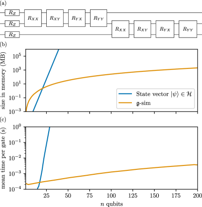
Figure 2: Performance benchmarks of $\mathfrak{g}$-sim. (a) Circuit used for the benchmark at $n=3$ qubits. The set of generators are presented in Eq. (18). Here, $R_{Z}$ denotes a rotation about the $Z$ axis, and $R_{\mu\nu}$ a rotation generated by the Pauli operator $\sigma^{\mu}\sigma^{\nu}$. We compare the memory (b) and compute time (c) requirements for state vector simulations (blue) and $\mathfrak{g}$-sim (orange) for the unitary shown in panel (a).

To demonstrate the power of $\mathfrak{g}{\text{-}}{\rm sim}$, we perform the following benchmarking task. We take the circuits $U(\bm{\theta})$ to be composed of a single layer of gates generated by the set of operators $\left(\bigcup_{\mu,\nu=x,y}\{\sigma^{\mu}_{j}\sigma^{\nu}_{j+1}\}_{j=1}^{n-1}\right)\cup\{\sigma^{z}_{j}\}_{j=1}^{n}$, where $\sigma^{\mu}_{j}$ (with $\mu=x,y,z)$ denotes the Pauli operators acting on the $j$-th qubit. In Fig. 2(a) we schematically show the circuit for $n=3$. The algebra associated with this evolution is

$$\mathfrak{g}_{0}={\rm span}_{\mathbb{R}}\left\langle\left(\bigcup_{\mu,\nu=x,y}\{i\sigma^{\mu}_{j}\sigma^{\nu}_{j+1}\}_{j=1}^{n-1}\right)\cup\{i\sigma^{z}_{j}\}_{j=1}^{n}\right\rangle_{\operatorname{Lie}}\!\!\!\!\!.$$ (18)

As shown in Ref. [35], a basis for $\mathfrak{g}_{0}$ is given by the set of Paulis

$$i\{\sigma^{z}_{j},\widehat{\sigma^{x}_{i}\sigma^{x}_{j}},\widehat{\sigma^{y}_{i}\sigma^{y}_{j}},\widehat{\sigma^{x}_{i}\sigma^{y}_{j}},\widehat{\sigma^{y}_{i}\sigma^{x}_{j}}\,|\,1\leqslant i<j\leqslant n\}\,,$$ (19)

where we used the notation $\widehat{A_{i}B_{j}}=A_{i}\sigma^{z}_{i+1}\cdots\sigma^{z}_{j-1}B_{j}$. This algebra is a representation of $\mathfrak{so}(2n)$, and hence its dimension is $\operatorname{dim}(\mathfrak{g}_{0})=n(2n-1)$ [35, 47]. In the GitHub repository of Ref. [48] we have reported these basis elements as well as their structure constants.

For the benchmarking task, we evaluate expectation values of random observables in the algebra $\mathfrak{g}_{0}$ for the state obtained by applying $U(\bm{\theta})$, with parameters uniformly sampled in the interval $[0,2\pi]$, to an input state $\rho^{(\operatorname{in})}=\ket{0}\!\bra{0}^{\otimes n}$. Since all the elements of the basis of $\mathfrak{g}_{0}$, given in Eq. (18), are Pauli operators, we can easily compute the expectation values in $\bm{e}^{(\operatorname{in})}$:

$$\Tr[\rho^{\operatorname{in}}G_{\alpha}]=\begin{cases}1\quad\text{if}\quad G_{\alpha}=\sigma^{z}_{j}\;(j=1,\ldots,n)\\ 0\quad\text{otherwise}\end{cases}\,.$$ (20)

In Fig. 2(b) we show benchmark results in terms of memory and compute time for $\mathfrak{g}{\text{-}}{\rm sim}$ and for full state-vector simulations methods. The benchmarks are computed on a single CPU core - using TensorFlow Quantum for state vector methods, and our Python implementation for $\mathfrak{g}{\text{-}}{\rm sim}$. Therein we can see that both memory and compute time scale as $\Omega(2^{n})$ for state vector methods, and as $\mathcal{O}(\operatorname{poly}(n))$ for $\mathfrak{g}$-sim. The exponential scaling of state-vector simulations makes simulations with $n\geqslant 30$ qubits intractable on the device used. However, using $\mathfrak{g}{\text{-}}{\rm sim}$ we are able to simulate systems of up to 200 qubits on a single core of a modern CPU. Further comments on the benchmarking procedure are given in Appendix D.1.

III Applications

Having presented the framework for $\mathfrak{g}{\text{-}}{\rm sim}$, we now explore its benefits in concrete problems. These include a study of the landscape of VQAs highlighting the overparametrization phenomenon (Sec. III.1), designing improved initialization of quantum circuits parameters (Sec. III.2), problems of circuit synthesis (Sec. III.3), and demonstration of the training of a quantum-phase classifier (Sec. III.4). These illustrate the broad range of applications that can be addressed with $\mathfrak{g}{\text{-}}{\rm sim}$.

We note that in all cases, we will implement $\mathfrak{g}{\text{-}}{\rm sim}$ based on either $\mathfrak{g}_{0}$ or subalgebras $\mathfrak{g}\subseteq\mathfrak{g}_{0}$ obtained by removing some of the generators from Eq. (18). In each section, we will specify which subalgebra of $\mathfrak{g}_{0}$ we will be working with, and a more detailed outline of the relevant subalgebras is given in Appendix E. We further remark that by definition, we will always be simulating circuits composed of single- and two-qubit gates with local connectivity - that is, circuits that could be implemented on most quantum hardware without incurring large compilation overhead. Details of these circuits are summarized in Table 1 of Appendix D.

III.1 Characterizing VQAs

VQAs aim to enable near-term quantum advantage by means of a hybrid quantum-classical training loop, where some of the problem difficulty is offloaded to an optimization problem on a classical co-processor. However, this optimization problem is difficult in general [49], and much remains to be learned about its scalability. Analytic study of optimization landscapes is difficult and limited in scope, while computational study is hindered by the exponential resource costs of state vector simulation. In this context, scalable classical simulations allow one to characterize trainability of VQAs at system sizes that would otherwise be intractable. A previous study has used free-fermion simulations for this purpose [19], but using $\mathfrak{g}$-sim expands the set of systems that can be studied. As a warm-up problem, we demonstrate the onset of overparametrization in VQE problems for the transverse field XY model at up to $n=50$ qubits.

III.1.1 Overparametrization in VQE

Overparametrization [50] is a surprising phenomenon in classical neural networks, where training a neural network with a capacity larger than that which is necessary to represent the training data distribution may lead to improved performance [51, 52, 53, 54] and even provable convergence results [55, 56], rather than to the overfitting and training difficulties one may naïvely expect. This phenomenon was generalized to quantum circuits in Ref. [43], where it was shown that the model capacity of circuits of the form Eq. (1) can be quantified by $\operatorname{dim}(\mathfrak{g})$. In turn, overparametrization is characterized by a ‘computational phase transition’ happening at a critical number of parameters $N_{p}^{(\text{crit})}\leqslant\operatorname{dim}(\mathfrak{g})$, below which the circuit is hard to train and above which it becomes easy to train. Exact values of this critical threshold $N_{p}^{(\text{crit})}$ are state-dependent, and often hard to assess analytically as they rely on the conjugation relationship between the initial state and the Lie algebra $\mathfrak{g}$ of the circuit. Thus, exact details of this phenomenon are best probed numerically. However, initial numerical demonstrations of the phenomenon were only provided for systems of 2-10 qubits [43]. Here we demonstrate the phenomenon in problems of up to 50 qubits.

III.1.2 Simulation results

To probe overparametrization, we consider a VQE task where the goal is to prepare the ground state of the TFXY model, whose Hamiltonian reads

$$H_{\text{TFXY}}=\sum_{j=1}^{n-1}(\sigma^{x}_{j}\sigma^{x}_{j+1}+\sigma^{y}_{j}\sigma^{y}_{j+1})+\sum_{j=1}^{n}b_{j}\sigma^{z}_{j}\,,$$ (21)

with coefficients $b_{j}$ randomly drawn from a Gaussian distribution $N(0,\xi^{2})$. As an ansatz for $U(\bm{\theta})$ we consider a Hamiltonian variational ansatz [57, 58] of the form in Eq. (1) with gate generators taken from the set $\{\sigma^{x}_{j}\sigma^{x}_{j+1},\sigma^{y}_{j}\sigma^{y}_{j+1}\}_{j=1}^{n-1}\cup\{\sigma^{z}_{j}\}_{j=1}^{n}$. We refer the reader to Appendix D for additional details on this circuit. One can verify that the dynamical Lie algebra associated with this set of generators is precisely $\mathfrak{g}_{0}$ in Eq. (18), such that we can use the structure constants reported in Ref. [48]. Given that $\operatorname{dim}(\mathfrak{g}_{0})=n(2n-1)$ and that the gates in $U(\bm{\theta})$ can be parallelized, then overparametrization is achievable with linear circuit depth. To solve the VQE problem, the parameters are optimized using the L-BFGS algorithm with the gradient evaluated according to Appendix C.1 to minimize the energy

$$E_{\operatorname{TFXY}}(\bm{\theta})=\bra{\bm{0}}U^{\dagger}(\bm{\theta})H_{\operatorname{TFXY}}U(\bm{\theta})\ket{\bm{0}}.$$ (22)

Note that the measurement operator $H_{\operatorname{TFXY}}$ is, by definition, fully supported within $\mathfrak{g}_{0}$. Moreover, since the initial state is the all zero state we can use the results in Eq. (20) to construct the vector $\bm{e}^{(\operatorname{in})}$. That is, we have all the ingredients for $\mathfrak{g}{\text{-}}{\rm sim}$.

For each of the system sizes probed, from $n=20$ to $50$ qubits, we perform optimization over circuits with a varied number of layers $L$ chosen to result in a number $N_{p}$ of circuit parameters spanning the range $[1,\operatorname{dim}(\mathfrak{g}_{0})]$, and random magnetic field amplitude $\xi=0.1$. For any of the circuits studied, optimizations are repeated over $50$ randomized initial parameter values and fields. Results of this study are reported in Fig. 3.

For a fixed system size of $n=50$ qubits, we display in Fig. 3(a) all the optimization traces. We observe the convergence behavior of the approximate training error $\epsilon_{\operatorname{TFXY}}(\bm{\theta})=(E_{\operatorname{TFXY}}(\bm{\theta})-E_{\operatorname{min}})/\|H_{\operatorname{TFXY}}\|_{\operatorname{HS}_{1}}$, where $E_{\operatorname{min}}$ is the lowest energy discovered by VQE across all depths and $\|\cdot\|_{\operatorname{HS}_{1}}=\|\cdot\|_{\operatorname{HS}}/2^{n}$ for $\|\cdot\|_{\operatorname{HS}}$ the Hilbert-Schmidt norm (i.e., we normalize the error relative to the energy scale of the Hamiltonian). Optimization traces exhibit a clear change in the hardness of the optimization problem as the depth of the circuits is varied. Below a critical threshold of $L\approx 6$ layers, we can see severe trainability issues where none of the optimization manages to converge to the ground state energy. However, for circuits with $L>6$ layers a sudden transition to trainability is observed and solutions converge towards the minimum energy. This phase transition in computational complexity indicates the onset of overparametrization.

More systematically, in Fig. 3(b), we study this phenomenon across varying system sizes $n$, from 20 to 50 qubits, and report the probability of convergence to $\epsilon_{\operatorname{TFXY}}<10^{-4}$ as a function of the number of circuit parameters in units of $\operatorname{dim}(\mathfrak{g}_{0})$. We observe that the transition to the trainable region (large convergence probability) occurs consistently across all system sizes at $N_{p}^{(\text{crit})}\approx 0.3\operatorname{dim}(\mathfrak{g})$ irrespective of $n$. This supports the analytic results of Ref. [43], and demonstrates the phenomenon of overparametrization at system sizes beyond what could be simulated with state vector simulations. Overall, such detailed analysis of VQA trainability at scale, that requires repetitions over many optimizations and many circuit sizes, is made possible by $\mathfrak{g}{\text{-}}{\rm sim}$.

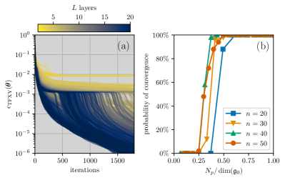
Figure 3: Overparametrization in large system sizes. (a) Convergence traces at $n=50$ qubits of the approximate training error $\epsilon_{\operatorname{TFXY}}(\bm{\theta})$. (b) The probability of converging to $\epsilon_{\operatorname{TFXY}}<10^{-4}$ for uniform random initialization of $\bm{\theta}$ as measured by 50 samples, at varied circuit depths, with corresponding number of parameters $N_{p}$ reported as a fraction of $\operatorname{dim}(\mathfrak{g}_{0})$, and for $n$ ranging from 20 to 50 qubits.

Overparametrization is crucial throughout the remainder of this work. It is provably achieved for circuits with $N_{p}\geqslant\operatorname{dim}(\mathfrak{g})$ parameters, and thus the tractably overparmeterizable models are those with $\operatorname{dim}(\mathfrak{g})\in\mathcal{O}(\operatorname{poly}(n))$. In cases where the relevant loss function depends entirely on observables supported by the algebra of the circuit (e.g., VQE with Hamiltonian variational ansatz [57, 59, 58, 60] or QAOA), circuits overparametrizable in polynomial depth are exactly those that can be efficiently simulated with $\mathfrak{g}$-sim. Hence, this phenomenon ensures that for any problem that is efficiently simulable in $\mathfrak{g}{\text{-}}{\rm sim}$, we can guarantee good trainability using a circuit of only polynomial gate-count. Crucially, this ensures a correctly trained prior model for our pre-training scheme (Sec. III.2), the ability to efficiently approximately compile unitaries in $\mathcal{G}$ to linear-depth circuits (Sec. III.3), and good trainability of QML models (Sec. III.4).

III.2 Pre-training quantum circuits

While the overparametrization regime guarantees trainability from arbitrary initial parameter values, in general cases where $\operatorname{dim}(\mathfrak{g})\in\Theta(4^{n})$ (i.e., cases where classical simulations are not possible anymore) it does not result in a scalable strategy. Indeed, trying to access the overparametrized regime would require constructing and training exponentially deep circuits, which is intractable for large problem sizes. Still, it is hoped that with an adequate choice of initial parameters one could train the circuits before the onset of overparametrization. Moreover, issues of barren plateaus [12, 61, 62, 42] (another crucial aspect of trainability) indicate exponentially vanishing gradients on average, but do not imply that the entire optimization landscape is flat. In fact, these are always accompanied by ‘narrow gorges’ in which minima are surrounded by regions of large gradient [63]. Hence, improvement in the trainability of quantum circuits can be achieved by means of ‘pre-training’ an ansatz such that its initial parameter values are sufficiently close to the optimal solution. As such, initialization by means of pre-training has received significant attention lately [20, 21, 22, 23, 24, 25, 26, 27, 28, 29, 30].

In this section, we demonstrate the use of $\mathfrak{g}{\text{-}}{\rm sim}$ for the initialization of VQAs. The idea (Sec. III.2.1) is to perform pre-training on a related auxiliary problem that induces a scalable Lie algebra, and to transfer the solution found as initial parameters for the circuit addressing the target problem. It is expected that the closer the auxiliary problem is to the target one, the more efficient such a transfer will be. As a first example (Sec. III.2.2), we study ground state preparation of the longitudinal-transverse field Ising model (LTFIM) via solving the transverse field Ising model (TFIM) in the first place. LTFIM only differs from TFIM by a few additional generators (the longitudinal fields) and we find substantial improvement both in terms of the fidelity of the ground states prepared and the magnitude of the initial gradients when utilizing pre-training. More surprisingly, we also show that in problems of QAOA (Sec. III.2.3), for which target and auxiliary tasks differ substantially, improved performances can still be achieved over a significant number of (but not all) problem instances.

III.2.1 Pre-training strategy with $\mathfrak{g}$-sim

Let us consider again here a VQE task where the goal is to prepare the ground state of an Hamiltonian $H$ that can be decomposed as $H=\sum_{j}c_{j}h_{j}$, where $c_{j}$ are real valued coefficients. We then define the Lie algebra $\mathfrak{g}_{\text{target}}=\langle\{ih_{j}\}\rangle_{{\rm Lie}}$, i.e., the algebra generated by the individual terms in $H$. The goal is to construct a circuit $U(\bm{\theta})$ to prepare the ground state of $H$ that is generated by some elements of $\mathfrak{g}_{\text{target}}$. In what follows, we will assume that $\operatorname{dim}(\mathfrak{g}_{\text{target}})\notin\mathcal{O}(\operatorname{poly}(n))$ (else the full VQE problem could be efficiently simulated with $\mathfrak{g}$-sim), meaning that $U(\bm{\theta})$ should not be constructed from a generating set of $\mathfrak{g}_{\text{target}}$. Hence, the scheme is as follows:

1. Identify a subset of the operators in $i\mathfrak{g}_{\text{target}}$, denoted as $\{h_{k}\}_{k}$ such that their Lie closure $\mathfrak{g}_{\text{aux}}=\langle\{ih_{k}\}\rangle_{{\rm Lie}}$, is a subalgebra $\mathfrak{g}_{\text{aux}}\subset\mathfrak{g}_{\text{target}}$ with $\operatorname{dim}(\mathfrak{g}_{\text{aux}})\in\mathcal{O}(\operatorname{poly}(n))$. Construct a proxy Hamiltonian $H_{\text{aux}}=\sum_{k}c_{k}h_{k}$. As we will see in the examples below, the choice of $c_{k}$ is informed by the task at hand.

2. On a classical computer, use $\mathfrak{g}{\text{-}}{\rm sim}$ to solve VQE on $H_{\text{aux}}$ using an ansatz generated by terms of $\mathfrak{g}_{\text{aux}}$ and with a number of parameters allowing for overparametrization.

3. Extend the trained ansatz with new gates generated by (some) of the terms in $\mathfrak{g}_{\text{target}}\setminus\mathfrak{g}_{\text{aux}}$. These new gates are initialized to the identity.

4. On a quantum computer, solve the VQE for $H$ starting from the ansatz constructed in step 3.

Although presented in the context of VQE, similar strategies could be applied to QML problems.

III.2.2 Pre-training VQE for the LTFIM

We begin by recalling that the LTFIM is a paradigmatic spin-chain model providing a prototypical example of a quantum phase transition. Its Hamiltonian reads

$$H_{\text{LTFIM}}=h_{xx}\sum_{j=1}^{n-1}\sigma^{x}_{j}\sigma^{x}_{j+1}+h_{z}\sum_{j=1}^{n}\sigma^{z}_{j}+h_{x}\sum_{j=1}^{n}\sigma^{x}_{j}\,,$$ (23)

where $h_{xx},h_{z},h_{x}\in\mathbb{R}$. It can be verified that the algebra $\mathfrak{g}_{\text{target}}$ obtained from the terms in $H_{\text{LTFIM}}$ has exponential dimension $\mathfrak{g}_{\text{LTFIM}}\in\Theta(4^{n})$ [42]. This renders it intractable in $\mathfrak{g}$-sim, induces a barren plateau for deep Hamiltonian variational circuits [42], and precludes efficient overparametrization [43], thus making application of the VQE to identify the ground state of Eq. (23) highly non-trivial.

Instead, by dropping some terms in $H_{\text{LTFIM}}$ we obtain the TFIM Hamiltonian, given by

$$H_{\text{TFIM}}=h_{xx}\sum_{j=1}^{n-1}\sigma^{x}_{j}\sigma^{x}_{j+1}+h_{z}\sum_{j=1}^{n}\sigma^{z}_{j}\,.$$ (24)

Notably, taking the Lie closure of the terms in $H_{\text{TFIM}}$ we obtain $\mathfrak{g}_{\text{aux}}\subseteq\mathfrak{g}_{0}$. Thus, we have successfully identified a subset of operators in $i\mathfrak{g}_{\text{target}}$ leading to a an algebra whose dimension is in $\mathcal{O}(\operatorname{poly}(n))$, making it overparametrizable [43] and classically tractable in $\mathfrak{g}{\text{-}}{\rm sim}$.

The pre-training strategy is now applied to ground state preparations of $H_{\text{LTFIM}}$. Following Sec. III.2.1, we begin by constructing an ansatz with $L=\operatorname{dim}(\mathfrak{g}_{0})$ and gates generated by terms appearing in $H_{\text{TFIM}}$:

$$U(\bm{\theta})=\prod_{l=1}^{\operatorname{dim}(\mathfrak{g}_{0})}e^{-i\theta_{l,1}\sum_{j=1}^{n-1}\sigma^{x}_{j}\sigma^{x}_{j+1}}e^{-i\theta_{l,2}\sum_{j=1}^{n}\sigma^{z}_{j}},$$ (25)

Parameters of the ansatz are initialized with random uniform values, and we train them to prepare the ground state of $H_{\text{TFIM}}$ using $\mathfrak{g}$-sim. Note that since the dynamical Lie algebra $\mathfrak{g}_{\text{aux}}$ associated with Eq. (25) is a subalgebra of $\mathfrak{g}_{0}$, we can use the structure constants we have pre-computed for $\mathfrak{g}_{0}$. This can be seen by noting that $e^{-i\theta_{l,1}\sum_{j=1}^{n-1}\sigma^{x}_{j}\sigma^{x}_{j+1}}=\prod_{j=1}^{n-1}e^{-i\theta_{l,1}\sigma^{x}_{j}\sigma^{x}_{j+1}}$, and that each gate generator is an element $\sigma^{x}_{j}\sigma^{x}_{j+1}$ of $\mathfrak{g}_{0}$. We detail further how to best make use of $\mathfrak{g}{\text{-}}{\rm sim}$ with generators that are sums of Pauli operators in Appendix B.2.

Once the parameters in Eq. (25) are trained to prepare the ground state of $H_{\text{TFIM}}$, we modify the circuit by inserting new gates generated by the remaining term of $H_{\text{LTFIM}}$, yielding the ansatz

$$U(\bm{\theta},\bm{\phi})=\prod_{l=1}^{\operatorname{dim}(\mathfrak{g}_{0})}\Big{[} e^{-i\theta_{l,1}\sum_{j=1}^{n-1}\sigma^{x}_{j}\sigma^{x}_{j+1}}e^{-i\theta_{l,2}\sum_{j=1}^{n}\sigma^{z}_{j}}$$

$$\quad e^{-i\phi_{l}\sum_{j=1}^{n}\sigma^{x}_{j}}\Big{]}\,.$$ (26)

The new gates are initialized to the identity by setting $\bm{\phi}=(0,0,\ldots)$, while the other gates retain their pre-trained values. Finally, we proceed by training the full ansatz of Eq. (26) to minimize the expectation value of $H_{\text{LTFIM}}$. Since $\dim(\mathfrak{g}_{\operatorname{LTFIM}})\in\Theta(4^{n})$, this last step must be performed using state vector simulations (we use TensorFlow Quantum [64]) thus limiting the system sizes that can be probed.

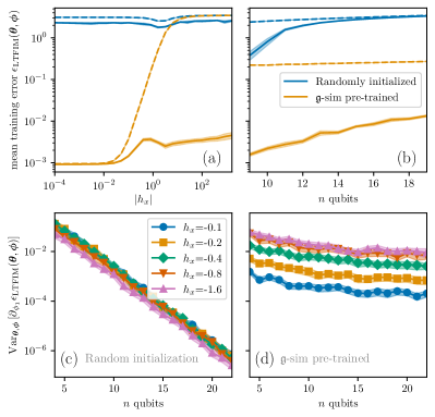
Figure 4: Pre-training VQE for LTFIM using $\mathfrak{g}$-sim. (a, b) Mean training error $\epsilon_{\operatorname{LTFIM}}(\bm{\theta},\bm{\phi})$ (Eq. (27)) for VQE with random initialization (blue) and pre-trained with $\mathfrak{g}$-sim (orange), (a) at $n=12$ qubits and varying longitudinal field strengths $h_{x}$ and (b) at field strength $h_{x}=-1.0$ and varying system sizes $n$. Dashed lines represent initial ansatz configurations, while solid lines represent trained ansätze. (c, d) Comparison of gradient variances at varying system size $n$ and longitudinal field strengths $h_{x}$ for (c) uniform random parameter initialization and (d) $\mathfrak{g}$-sim pre-training. Shaded bars represent bootstrapped 95% confidence intervals.

In Fig. 4, we report a comparison of the pre-training strategy discussed versus uniform random initialization of the circuit parameters, for Hamiltonians with $h_{z}=-1$ and $h_{xx}=1$. As can be seen in Figures 4(a, b), pre-training yields improvements by several orders of magnitude in terms of the error

$$\epsilon_{\operatorname{LTFIM}}(\bm{\theta},\bm{\phi})=\frac{\bra{\bm{0}}U^{\dagger}(\bm{\theta},\bm{\phi})H_{\text{LTFIM}}U(\bm{\theta},\bm{\phi})\ket{\bm{0}}-E_{\text{min}}}{\|H_{\text{LTFIM}}\|_{\operatorname{HS}_{1}}},$$ (27)

where $E_{\text{min}}$ is the ground state energy of $H_{\text{LTFIM}}$ obtained by exact diagonalization.

In Fig. 4(a), we compare these errors as a function of the longitudinal field strength $|h_{x}|$. The prepared state resulting from the pre-training strategy (with errors depicted as an orange dashed line) becomes a poorer approximation to the ground state as $|h_{x}|$ increases, and even sometimes at par with random initialization (blue dashed line). Still, after the final step of optimization (with errors depicted as plain lines) we found pre-training to consistently enable accurate ground state preparation of $H_{\text{LTFIM}}$. Across all the values of $h_{x}$ studied, the pre-training strategy is the most favorable initialization.

In Fig. 4(b), we report final errors scaling with the system size $n$, noting that the randomly initialized circuits quickly become untrainable as $n$ increases while the pre-trained ansatz only exhibits mild decline in trainability.

In addition to these improved errors, we observe a mitigation of the barren plateau effect. Due to the exponential dimension of $\mathfrak{g}_{\operatorname{LTFIM}}$, in the case of random initialization one would expect gradient variance scaling as [42]

$$\operatorname{Var}_{\bm{\theta},\bm{\phi}}\left[\partial_{\phi_{m}}\epsilon_{\text{LTFIM}}(\bm{\theta},\bm{\phi})\right]\in\mathcal{O}\left(\frac{1}{2^{n}}\right),$$ (28)

thus necessitating $\Theta(2^{n})$ circuit repetitions to distinguish small gradient values from statistical shot noise. This is verified numerically in Fig. 4(c) which, over varied values of the field $h_{x}$, showcases exponentially vanishing gradients. However, in the case of $\mathfrak{g}$-sim pre-training, we can see in Fig. 4(d), that the gradient variances vanish at a much slower rate in $n$, effectively mitigating appearance of the barren plateau effect and thus extending the scalability of VQE on this system.

III.2.3 Pre-training QAOA

The quantum approximate optimization algorithm (QAOA) is a VQA that attempts to solve combinatorial optimization problems [65]. Specifically, we consider here its use to approximate solutions of MaxCut problems. We recall that given a graph $G$ with edges $E$ and vertices $V$, the maximum cut (MaxCut) problem is to find a partition of V into two sets $S$ and $T$ that maximizes the number of edges $e\in E$ having endpoints in both $S$ and $T$. Encoding a partition as a bitstring $\bm{z}\in\{0,1\}^{n}$, its fitness for the MaxCut problem can be quantified by the approximation ratio $r$ defined as

$$r(\bm{z})\equiv\frac{C(\bm{z})}{\operatorname*{arg\,max}_{\bm{z}}C(\bm{z})},\;C(\bm{z})\equiv\sum_{(m,l)\in E}z_{m}(1-z_{l})\,.$$ (29)

For general graph problems, finding an exact MaxCut solution is NP-hard. Still, the Goemans-Williamson (GW) algorithm [66] allows one to efficiently find an approximation with a ratio of at least $r_{\rm GW}\approx 0.878$. To obtain quantum advantage with QAOA, one must outperform this threshold.

QAOA recasts a MaxCut problem as a VQE problem, where the goal is to find the ground state of the phase Hamiltonian

$$H_{G}=\frac{1}{2}\sum_{(m,l)\in E}(\sigma^{z}_{m}\sigma^{z}_{l}-I)\,,$$ (30)

that depends on the underlying graph $G$. To prepare such a ground state, one applies a circuit

$$U(\bm{\beta},\bm{\gamma})=\prod_{m=1}^{p}e^{-i\beta_{m}H_{M}}e^{-i\gamma_{m}H_{G}}\,,$$ (31)

where $H_{M}=\sum_{j=1}^{n}\sigma^{x}_{j}$ is the so-called mixing Hamiltonian, to an initial state $\ket{+}^{\otimes n}$. By optimizing the variational parameters ($\bm{\beta}$ and $\bm{\gamma}$) to minimize the expectation value $\langle+|^{\otimes n}U^{\dagger}(\bm{\beta},\bm{\gamma})H_{P}U(\bm{\beta},\bm{\gamma})|+\rangle^{\otimes n}$ and measuring the resulting state in the computational basis, one may construct approximate solutions to MaxCut. In correspondence to Eq. (29), the approximation ratio of the solution generated by QAOA is defined as

$$r(\bm{\beta},\bm{\gamma})\equiv\frac{\bra{+}^{\otimes n}U^{\dagger}(\bm{\beta},\bm{\gamma})H_{G}U(\bm{\beta},\bm{\gamma})\ket{+}^{\otimes n}}{\bra{\psi_{\operatorname{GS}}}H_{G}\ket{\psi_{\operatorname{GS}}}}\,,$$ (32)

where $\ket{\psi_{\operatorname{GS}}}$ is the ground state of the Hamiltonian $H_{G}$.

While optimal parameters can be identified for $p=1$ [67], optimizing them for larger depth (where improved solutions can be found) remains a challenge. Indeed, several works show that general problem instances are likely to experience unfavorable optimization landscapes in the absence of any special underlying structure [68, 69]. These point toward the necessity of finding pre-training strategies for deep-circuit QAOA.

It has been reported that for most choices of $G$ the Lie algebra associated with Eq. (31) will have dimension in $\Omega(2^{n})$ [42, 47]. Hence, to apply our pre-training strategy, we need to identify an algebra with polynomial dimension that is related to the original problem. For the circuit of Eq. (31), this is the case for the path graph $G=P_{n}$ on $n$-vertices. For such a choice, the Lie algebra $\mathfrak{g}_{\text{QAOA,}P_{n}}={\rm span}\langle\{iH_{P_{n}},iH_{M}\}\rangle_{\operatorname{Lie}}$ is such that (up to a change of basis, where the Pauli $\sigma^{x}$ and $\sigma^{z}$ are interchanged) $\mathfrak{g}_{\text{QAOA,}P_{n}}\subset\mathfrak{g}_{0}$, and therefore has $\operatorname{dim}(\mathfrak{g}_{\text{QAOA,}P_{n}})\in\mathcal{O}(\operatorname{poly}(n))$ (see Appendix E). Hence, we can again use the structure constants of $\mathfrak{g}_{0}$, and start by training such circuit for $p=\operatorname{dim}(\mathfrak{g}_{\text{QAOA,}P_{n}})$.

The pre-trained parameters $\bm{\beta}$ and $\bm{\gamma}$ can then be used to initialize the modified ansatz

$$\begin{split}U_{G}(\bm{\alpha},\bm{\beta},\bm{\gamma})=\prod_{l=1}^{p}\Big{[}&e^{-i\beta_{l}H_{M}}e^{-i\gamma_{l}H_{P_{n}}}e^{-i\alpha_{l}H_{G}}\Big{]}\end{split}$$ (33)

for any general graph $G\neq P_{n}$, with the new parameters initialized to $\bm{\alpha}=(0,0,\ldots)$. We then train the parameters $\bm{\alpha}$, $\bm{\beta}$, $\bm{\gamma}$ to minimize the expectation value of $H_{G}$.

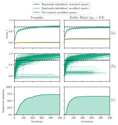
Figure 5: Pre-training QAOA using $\mathfrak{g}$-sim. Performances of QAOA on MaxCut at $n=16$ qubits for the standard randomly-initialized QAOA ansatz (blue), the modified randomly-initialized ansatz (orange), and the modified ansatz pre-trained with $\mathfrak{g}$-sim (green). Comparisons are made across ensembles of 200 random 3-regular graphs (left panels) and 200 Erdös-Réyni graphs with edge probability $p_{E}=0.3$ (right panels). We compare (a) the mean approximation ratios $r$ (shaded bars are bootstrapped 95% confidence intervals), (b) individual training trajectories, and (c) the fraction of solutions outperforming the GW threshold (reported as an horizontal dashed line).

We study the benefits of this pre-training at $n=16$ qubits on random 3-regular graphs and Erdös-Rényi graphs with edge probability $p_{E}=0.3$. Results are reported in Fig. 5, showing that pre-training significantly outperforms randomly-initialized QAOA circuits.

In terms of the mean approximation ratio $r$ (Fig. 5(a)), both randomly-initialized strategies vastly under-perform the GW threshold $r_{\rm GW}$ (horizontal dashed line), while the pre-training strategy achieves comparable average performance. More strikingly, when looking at details of the approximation ratios $r$ of the individual graph problems (Fig. 5(b)), we find a majority of individual graphs for which $r>r_{\rm GW}$, and the rest for which it is at par with random initialization.

Overall, the fraction of solutions that improve on the GW threshold (Fig. 5(c)) converges to $72.5\%$ for 3-regular graphs, and $66.5\%$ for $p_{E}=0.3$ Erdös-Rényi graphs. On the other hand, no randomly-initialized circuits achieved better than this threshold. This indicates that $\mathfrak{g}$-sim pre-training is advantageous for QAOA on a substantial fraction of random graphs, even for a relatively crude initialization strategy. Further improvements could likely be achieved by more carefully aligning the path graph $P_{n}$ along $G$, adaptively transforming the ansatz and cost, or resorting to another polynomially-size algebra for the pre-training.

III.3 Circuit synthesis

Until now, we have been concerned with tasks of state-preparation. We now address more difficult problems of unitary compilation. Here, we seek to use $\mathfrak{g}{\text{-}}{\rm sim}$ to identify the parameters of an ansatz circuit $U(\bm{\theta})\in\mathcal{G}$ of the form Eq. (1) to implement a target unitary $V\in\mathcal{G}$. Despite the fact that both the target and circuit must belong to a unitary Lie group whose associated Lie algebra is of polynomial dimension, such strategy can already enlarge the reach of $\mathfrak{g}{\text{-}}{\rm sim}$. In particular, previous uses of $\mathfrak{g}{\text{-}}{\rm sim}$ (as reported in Results 1 & 16) were restricted to certain initial states and observables, but our circuit synthesis compilation goes beyond these cases. Now, $\mathfrak{g}{\text{-}}{\rm sim}$ can be used to classically compile a polynomial-gate-count circuit, and then implement it on a quantum computer to evaluate the evolution of any observable or state. More generally, the unitary to be synthesized could be part of a larger protocol such that the initial state or observable may not even be known beforehand. Finally, we note that there may be utility in compiling random unitaries corresponding to polynomially sized Lie algebras, as sampling from the output of some of these circuits have strong hardness guarantees that can be used to demonstrate quantum advantage [70].

The scheme proposed is presented in Sec. III.3.1. We probe its convergence properties for random targets in Sec. III.3.2 displaying polynomial optimization effort in most cases. However, as documented in Sec. III.3.3, given that we work in a reduced representation of the algebra, issues of faithfulness can arise and compromise compilation. Still, we provide a strategy to overcome this issue. Resorting to this strategy we demonstrate exact compilations with $\mathfrak{g}{\text{-}}{\rm sim}$ in a task of dynamical evolution in Sec. III.3.4.

III.3.1 Variational compilation of unitaries in $\mathfrak{g}{\text{-}}{\rm sim}$

In variational circuit compilation, we typically seek to train the parameters of an ansatz circuit $U(\bm{\theta})$ to approximate some target unitary $V$. Existing techniques for compiling variational circuits to target unitaries usually seek to minimize the cost

$$\mathcal{L}_{\text{HST}}(U(\bm{\theta}),V)\equiv 1-\frac{1}{d^{2}}|\Tr(U^{\dagger}(\bm{\theta})V)|^{2},$$ (34)

that has computational complexity growing quadratically with $d=2^{n}$ rendering it quickly classically intractable, and thus would require evaluation on a quantum computer for even modest system sizes. In this situation, evaluation of Eq. (34) could rely on the Hilbert-Schmidt test [71, 72] or on estimation via state sampling [73, 74]. In any case, these assume implementation of the target $V$ in the first place, which is often unrealistic.

In contrast, provided a description of $V\in\mathcal{G}$ with dimension of the associated Lie algebra $\operatorname{dim}(\mathfrak{g})\in\mathcal{O}(\operatorname{poly}(n))$, the present approach to compilation can be performed entirely on a classical computer with $\mathcal{O}(\operatorname{poly}(n))$ resources. To that intent, we propose the loss function

$$\mathcal{L}_{\mathfrak{g}}(U(\bm{\theta}),V) \equiv\frac{1}{2\operatorname{dim}(\mathfrak{g})}\|\bar{\bm{U}}(\bm{\theta})-\bar{\bm{V}}\|^{2}_{\operatorname{HS}}$$

$$=1-\frac{1}{\operatorname{dim}(\mathfrak{g})}\operatorname{Re}\left[\Tr(\bar{\bm{U}}^{T}(\bm{\theta})\bar{\bm{V}})\right],$$ (35)

where $\|\cdot\|_{\operatorname{HS}}$ is again the Hilbert-Schmidt norm and $\bar{\bm{U}}(\bm{\theta})\equiv\Phi^{\operatorname{Ad}}_{\mathcal{G}}(U(\bm{\theta}))$, $\bar{\bm{V}}\equiv\Phi^{\operatorname{Ad}}_{\mathcal{G}}(V)$ are the adjoint representations of $U(\bm{\theta})$ and $V$, respectively. Gradients of $\mathcal{L}_{\mathfrak{g}}$ can be calculated efficiently, with implementation details provided in Appendix C.2.

In effect, $\mathcal{L}_{\mathfrak{g}}$ measures how accurately $U(\bm{\theta})$ approximates the evolution of the expectation values $\langle G_{\alpha}\rangle$ under evolution by $V$ for all initial states. Although the Hilbert-Schmidt loss $\mathcal{L}_{\text{HST}}$, in Eq. (34), and its adjoint-space version $\mathcal{L}_{\mathfrak{g}}$, in Eq. (35), are similar in form, we highlight that $\mathcal{L}_{\mathfrak{g}}$ is sensitive to global phase differences between $\bar{\bm{U}}(\bm{\theta})$ and $\bar{\bm{V}}$, whereas $\mathcal{L}_{\text{HST}}$ is not sensitive to global phase differences between $U(\bm{\theta})$ and $V$. This is because global phase differences in the full Hilbert space are nonphysical, whereas global phase differences in the adjoint representation correspond to a sign flip on all basis observables, which is indeed physical. As we shall see (Sec. III.3.3) related subtleties may compromise our ability to perform faithful compilation. For now we leave these aside, and assess convergence of optimizations with the loss in Eq. (35) for random target unitaries.

III.3.2 Compiling random unitaries

We first benchmark our compilation scheme against random unitaries in $\mathcal{G}_{0}=e^{\mathfrak{g}_{0}}$, which is the most general and demanding task for this scheme. Any unitary in $\mathcal{G}$ may be written in the form

$$V=e^{-iT\sum_{\alpha}(\bm{w})_{\alpha}G_{\alpha}}\,,$$ (36)

where we fix $|\bm{w}|_{2}=1$ such that $T$ parametrizes the effective duration of the corresponding dynamics. To generate the weights we sample a matrix from a Haar distribution over the orthogonal group and set the weight vector $\bm{w}$ equal to one of its columns (potentially padding with zeros to account for elements of the basis not present in the sum).

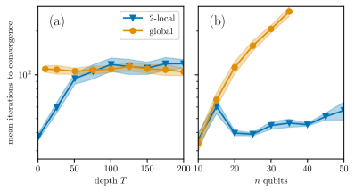
Figure 6: Scaling properties of circuit compilation with $\mathfrak{g}$-sim. We compare the mean number of iterations to converge to a loss (defined in Eq. (35)) $\mathcal{L}_{\mathfrak{g}}<10^{-3}$ for random target unitaries (defined in Eq. (36)) with varied levels of locality, including 2-local and global generators. Results for (a) varying duration $T$ at $n=20$ qubits, and for (b) varying system size $n$ at duration $T=10$. The Shaded bars depict bootstrapped 95% confidence intervals. The scaling of the iterations number is found to be polynomial in $n$ and $T$.

In general, Eq. (36) involves highly non-local interactions, since many elements of $\mathfrak{g}_{0}$ are non-local Pauli strings (see Eq. (19)). By excluding greater-than-$k$-local $G_{\alpha}$ from Eq. (36), we can refine our study to $k$-local Hamiltonian dynamics.

We test our scheme by compiling global and 2-local dynamics, both with the 2-local ansatz of Fig. 2(a), (see Appendix D for more details), using $L=\left\lceil{2\operatorname{dim}(\mathfrak{g})/K}\right\rceil$ layers, with $K$ the number of generators, ensuring overparametrization. In Fig. 6, we show that the compilation of random unitaries $V\in\mathcal{G}_{0}$ performs and scales well. At fixed $n=20$ qubits (Fig. 6(a)), the convergence requirements (measured as the number of optimization iterations required for convergence) plateau to a constant value irrespective of $T$, indicating that our approach allows fixed-circuit-depth Hamiltonian simulation for arbitrary evolution time. We note that this phenomenon was demonstrated in Ref. [75] on related systems, but with different methods and only targeting local dynamics.

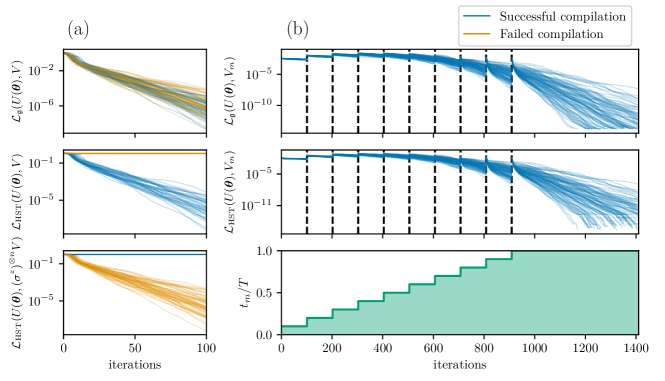
Figure 7: Successfully compiling circuits in an algebra with non-trivial group center elements. (a) Although the classical loss function $\mathcal{L}_{\mathfrak{g}}(U(\bm{\theta}),V)$ can be efficiently minimized (Fig. 6), this is a necessary but insufficient condition to minimize the Hilbert-Schmidt loss function $\mathcal{L}_{\text{HST}}$, and thus to faithfully compile a target unitary $V$. We train a linear-depth ansatz $U(\bm{\theta})$ (see Fig. 2(a)) initialized with uniform random parameters to minimize $\mathcal{L}_{\mathfrak{g}}(U(\bm{\theta}),V)$ at $T=1$ and $n=10$. Although $\mathcal{L}_{\mathfrak{g}}$ is successfully minimized in all instances (top panel), $\mathcal{L}_{\text{HST}}$ is only minimized in approximately half the instances, and rather maximized otherwise (middle panel). In all cases where the compilation fails, the optimized ansatz instead approximates $(\sigma^{z})^{\otimes n}V$ (bottom panel). (b) The scheme outlined in Sec. III.3.3 successfully rectifies this issue. The ansatz is initialized at $\bm{\theta}=\bm{0}$, and compiled to a sequence of intermediate targets $V_{m}$ corresponding to increased $t_{m}$ from 0 to T (bottom panel), with the parameters obtained from compiling a target used to initialize the next . For sufficiently small time steps $\Delta t_{m}$, successfully minimizing $\mathcal{L}_{\mathfrak{g}}$ (top panel) ensures minimization of $\mathcal{L}_{\text{HST}}$ (middle panel) and thus faithful compilation of the final target $V$.

At fixed $T$ (Fig. 6(b)), the number of steps to converge appears constant in $n$ for 2-local targets, and polynomial in $n$ for global ones. The case of global targets with small duration $T$ is detailed further in Appendix F.1. Overall, this demonstrates that our methods can efficiently minimize the loss $\mathcal{L}_{\mathfrak{g}}$ on an overparametrized ansatz for a range of random unitaries in $\mathcal{G}_{0}$ with varying locality, system size $n$, and dynamics duration $T$, providing a strong foundation for our compilation scheme.

III.3.3 Faithfulness of compilation

Although we saw consistent convergence with respect to $\mathcal{L}_{\mathfrak{g}}$ (Fig. 6), one should question whether minimizing $\mathcal{L}_{\mathfrak{g}}$ is sufficient for unitary compilation. It can be seen from Eq. (35) that $\mathcal{L}_{\mathfrak{g}}$ is a faithful loss function for unitary training iff $\Phi^{\operatorname{Ad}}_{\mathcal{G}}$ is a faithful representation.

As discussed in Sec. II.2, faithful representation $\Phi^{\operatorname{ad}}_{\mathfrak{g}}$ of the Lie algebra does not guarantee faithful representation $\Phi^{\operatorname{Ad}}_{\mathcal{G}}$ of the Lie group. In particular, we have already seen in Eq. (10) that for unitaries $W\in Z(\mathcal{G})$ (i.e., for unitaries in the center of the group), it is the case that $\Phi^{\operatorname{Ad}}_{\mathcal{G}}(W)=I$ such that $\Phi^{\operatorname{Ad}}_{\mathcal{G}}(WV)=\Phi^{\operatorname{Ad}}_{\mathcal{G}}(V)$. That is, in the adjoint representation one cannot distinguish $V$ from $WV$. For the case of $\mathfrak{g}_{0}$, the center is $Z(\mathcal{G})=\{(\sigma^{z})^{\otimes n},I\}$ up to a global phase (as detailed in Appendix F.2).

Such an issue can indeed be seen in our numerics. In the first row of Fig. 7(a) we report systematic success in minimizing $\mathcal{L}_{\mathfrak{g}}$. However, as can be distinguished by the loss $\mathcal{L}_{\text{HST}}$, only half of the optimizations yields the correct target $V$ while the other half rather yields the unitary $(\sigma^{z})^{\otimes n}V$ (second and third row). To guarantee successful compilation of $V$, one must either ensure convergence to the manifold of correct solutions, or be able to flag when an error has occurred such that it could be corrected (i.e., by applying an additional unitary $(\sigma^{z})^{\otimes n}$). We now detail a strategy achieving the former.

Any unitary target $V\in\mathcal{G}$ may be written in the form $V=e^{-iTH}$ with $iH\in\mathfrak{g}$ as in Eq. (36). Rather than directly aiming for the compilation of $V$, we consider a family of intermediary targets $V_{m}=e^{-iHt_{m}}$ for increasing steps $t_{m}\in[0,T]$, with $t_{0}=0$. We then solve the corresponding compilation problems $\bm{\theta}_{m}=\operatorname*{arg\,min}_{\bm{\theta}}\mathcal{L}_{\mathfrak{g}}(U(\bm{\theta}),V_{m})$ sequentially, with $\bm{\theta}$ initialized to $\bm{\theta}_{m-1}$ at each step. For sufficiently small $\Delta t_{m}=t_{m}-t_{m-1}$, it is expected that no jump between solution manifolds will occur. Crucially, given that $V_{0}=I$, we can ensure that we start in the correct manifold by setting $\bm{\theta}_{0}=\bm{0}$ such that $U(\bm{\theta}_{0})=I$ (rather than $(\sigma^{z})^{\otimes n}$) .

Viability of the proposed scheme is confirmed numerically and reported in Fig. 7(b). For all the random unitaries $V$ assessed, the optimization concludes with parameters replicating accurately the desired target, as evidenced by the low values of $\mathcal{L}_{\text{HST}}(U(\bm{\theta}),V)<10^{-6}$. This demonstrates that faithful compilation is possible even when the cost function $\mathcal{L}_{\mathfrak{g}}$ is not faithful.

III.3.4 Application to dynamical simulation

As noted in Sec. III.3.2, given a Hamiltonian supported by a Lie algebra $\mathfrak{g}$ with $\operatorname{dim}(\mathfrak{g})\in\mathcal{O}(\operatorname{poly}(n))$, our scheme enables compilation in polynomial-depth circuits of the corresponding time-evolution operators. This allows the study of dynamics of observables not supported by $\mathfrak{g}{\text{-}}{\rm sim}$ and arbitrary states, which are in general not classically tractable. Here we demonstrate the utility of our scheme by synthesizing circuits for the Hamiltonian time-evolution of the TFXY spin chain of Eq. (21) with open boundary conditions and random local magnetic fields $b_{j}$ drawn from $N(0,\xi^{2})$. This Hamiltonian supports the phenomenon of Anderson localization [76], and has previously been utilized to demonstrate related compilation techniques based on Cartan decomposition [75].

We aim to train an ansatz $U(\bm{\theta}_{t_{m}})$ to approximate $V_{t_{m}}\equiv e^{-i{t_{m}}H_{\text{TFXY}}}$ at a range of discrete times $t_{m}\in[0,200]$. For each $t_{m}$, the ansatz has a structure

$$U(\bm{\theta})=\prod_{l=1}^{L}\Big{[} \prod_{j=1}^{n-1}e^{-i\theta_{l,(n+2j+1)}\sigma^{x}_{j}\sigma^{x}_{j+1}}e^{-i\theta_{l,(n+2j)}\sigma^{y}_{j}\sigma^{y}_{j+1}}$$

$$\quad\prod_{j=1}^{n}e^{-i\theta_{l,j}\sum_{j=1}^{n}\sigma^{z}_{j}}\Big{]}\,,$$ (37)

One can verify that the dynamical Lie algebra associated with this circuit is again $\mathfrak{g}_{0}$ as defined in Eq. (19), meaning that we can again utilize the structure constants we have already computed. At this point we note that while $U(\bm{\theta})$ has the exact same structure as that of a first-order Trotterization of any of the $V_{t_{m}}$ unitaries, each term of the Hamiltonian is associated with an independent trainable parameter in $U(\bm{\theta})$. This fact is important as $U(\bm{\theta})$ is not trying to learn a Trotterized version of $V_{t_{m}}$. In fact, because we use $\mathfrak{g}{\text{-}}{\rm sim}$, we do not need to ever perform a Trotterization of the target unitary, as $V_{t_{m}}$ can be compiled exactly for all evolution times $t_{m}$. This is due to the fact that one can efficiently compute the adjoint representation $\Phi^{\operatorname{Ad}}_{\mathcal{G}}(V_{t_{m}})=e^{-it_{m}\Phi^{\operatorname{ad}}_{\mathfrak{g}}(H_{\text{TFXY}})}$ on a classical computer. This is advantageous compared to variational compilation schemes for time evolution that necessitate the target to be implementable on a quantum device in the first place (often achieved by means of a Trotter approximation [77, 74] and therefore introducing approximation errors).

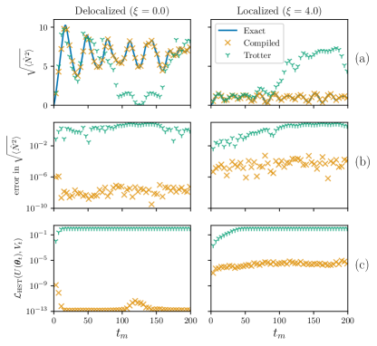
Figure 8: Compiling Hamiltonian dynamics with $\mathfrak{g}$-sim. Dynamics of a single-spin-flip excitation in a TFXY spin chain (Eq. (21) with $n=12$) in the absence of magnetic fields ($\xi=0$, left panels) and with random fields inducing Anderson localization ($\xi=4$, right panels). The exact dynamics (blue) is compared to the dynamics yielded by our compilation scheme (orange X), and first-order Trotterization (green Y). The compilation scheme accurately showcases Anderson localization, reproducing the RMS position $\sqrt{\hat{N}^{2}}$ of the excitation (a) with low errors (b), while Trotterization quickly diverges beyond small simulation times. Furthermore, comparison of the compiled unitaries to the exact time-evolution operators by means of the Hilbert-Schmidt test $\mathcal{L}_{\text{HST}}$, show small errors at all times (c), guaranteeing faithful dynamics of all observables.

For the sake of concreteness, we focus on the dynamics of a single-spin-flip initial state $\ket{\downarrow\uparrow\uparrow\uparrow\uparrow\uparrow\uparrow\uparrow\uparrow\uparrow\uparrow\uparrow}$ for $n=12$ qubits. In the absence of a magnetic field ($b_{j}=0$ for all $j$) this excitation diffuses throughout the system, but a disordered field ($\xi>0$) restricts this diffusion (Anderson localization). Following the example of Ref. [75], we study the position operator for the excitation

$$\hat{N}=\sum_{j=1}^{n}(j-1)\frac{1-\sigma^{z}_{j}}{2}\,,$$ (38)

whose moments provide a key signature of Anderson localization. In particular, for this system the $p$-th moment $\langle|\hat{N}|^{p}\rangle$ admits a time-independent upper bound [75, 78]. Note that $\hat{N}^{2}$ is expressible as a linear combination of elements in the algebra ($\sigma_{j}^{z}$) and product of elements in the algebra ($\sigma_{j}^{z}\sigma_{j^{\prime}}^{z}$), and thus is precisely of the form in Eq. (17). Moreover, given that the algebra is composed of Pauli operators, and since the initial state is separable, we can readily compute the entries of the vector $\bm{e}^{(\operatorname{in})}$ and the matrix $\bm{E}^{(\operatorname{in})}$. Hence, the $p=2$ moment can be efficiently computed with $\mathfrak{g}{\text{-}}{\rm sim}$. As noted above, larger moments quickly become intractable. Furthermore, we stress that our choice of a classically-tractable system size ($n=12$ qubits) is purely to enable us to compute the loss $\mathcal{L}_{\text{HST}}(U(\bm{\theta}_{t_{m}}),V_{t_{m}})$ for verification of correct unitary compilation. In general, our scheme can achieve compilation at larger system sizes (e.g., $n=50$ qubits in Fig. 6).

We compile the time-evolution operators for the case of no magnetic field ($\xi=0$) and of a disordered magnetic field ($\xi=4$) with a Hamiltonian renormalized as $H_{\text{TFXY}}\to\frac{H_{\text{TFXY}}}{\|H_{\text{TFXY}}\|_{\operatorname{HS}_{1}}}$ to eliminate any norm dependence of the dynamics. Our ansatz is determined by Eq. (37) and is composed of $L=17$ layers, which is overparametrized to ensure trainability. In line with the strategy previously discussed, the circuit is first initialized with $\bm{\theta}_{t_{0}}=\bm{0}$, and thereafter initialized with $\bm{\theta}_{t_{m}}$ according to the parameters found in the ${t_{m-1}}$ step of optimization.

In Fig. 8, we report a comparison between the compiled dynamics and a first-order Trotterization at the same depth (i.e., identical circuit structure with $\theta_{lk}=t/L$). We find that, despite using identical circuit structures, our scheme outperforms Trotterization by several orders of magnitude. Looking at the dynamics of the position operator $\sqrt{\hat{N}^{2}}$ (Fig. 8(a)) one can see that Trotterization fails to reproduce results beyond $t\approx 60$ while our scheme continues to track them accurately at any of the times considered, with errors smaller than $10^{-6}$ (Fig. 8(b)). More generally, we find that the compiled unitaries reflect accurately the true time-evolution with $\mathcal{L}_{\operatorname{HST}}(U(\bm{\theta}_{t}),V_{t})<10^{-5}$ (Fig. 8(c)), thus guaranteeing that the compiled circuits can faithfully reproduce the dynamics of all observables, not just those supported by $\mathfrak{g}$ and products thereof. Furthermore, the errors entailed by the compiled circuit do not appear to vary substantially in the duration of the dynamics. Overall, this shows that for time-evolution operators whose associated Lie algebra $\mathfrak{g}$ has $\operatorname{dim}(\mathfrak{g})\in\mathcal{O}(\operatorname{poly}(n))$, our $\mathfrak{g}$-sim compilation schemes can determine a much more efficient circuit implementation than standard Trotterization.

III.4 Supervised quantum machine learning

As a final demonstration, we employ $\mathfrak{g}{\text{-}}{\rm sim}$ for the training of a quantum-phase classifier, showcasing its applicability in the context of QML. Despite being trained fully classically on tractable states, such a classifier could then be employed to classify unknown quantum states. Provided that meaningful training data points and quantum models can be found in algebras with polynomial dimension, such schemes could find utility in real experiments. Additionally, in the spirit of Sec. III.2, our $\mathfrak{g}{\text{-}}{\rm sim}$ approach could form the basis of approximate quantum models that are then refined on a quantum computer.

III.4.1 Supervised QML

In general problems of supervised QML one assumes repeated access to a training dataset $\mathcal{S}=\{(\rho_{s},y_{s})\}_{s=1}^{N}$ consisting of of $N$ pairs of states $\rho_{s}$ together with labels $y_{s}=F(\rho_{s})$ that have been assigned by an unknown underlying function $F$. The task is to learn parameters $\bm{\theta}$ of a function $h_{\bm{\theta}}$ aiming at approximating $F$ as accurately as possible. Upon successful training, it is then possible to accurately predict the labels of previously unseen states.

As typical in tasks of QML, we consider a model $h_{\bm{\theta}}$ that relies on the expectation value of an observable $O$ after application of a circuit $U(\bm{\theta})$. That is, on $\ell_{\bm{\theta}}(\rho_{s})=\Tr[OU(\bm{\theta})\rho_{s}U^{\dagger}(\bm{\theta})]$. Training relies upon minimization of a mean-squared error loss function, defined here as

$$\mathcal{L}(\bm{\theta})=\frac{1}{N}\sum_{s=1}^{N}(y_{s}-\ell_{\bm{\theta}}(\rho_{s}))^{2}\,.$$ (39)

III.4.2 Training a binary quantum-phase classifier

For our numerical study, we apply the $\mathfrak{g}{\text{-}}{\rm sim}$ framework to the classification of ground states across a phase transition of the TFIM, in Eq. (24), at system size $n=50$ qubits. We consider parameters $h_{z},h_{xx}\in[0,1]$ in order to focus on a single phase transition (binary classification). For $h_{z}/h_{xx}>1$, the ground state is in the disordered phase, while for $h_{z}/h_{xx}<1$ it is in the antiferromagnetic phase. Furthermore, to ensure that the problem is non-trivial, we ‘disguise’ the TFIM according to a random $V\in\mathcal{G}$ (Eq. (36) with $T=10$) such that

$$H_{\text{disguised}}=VH_{\text{TFIM}}V^{\dagger}.$$ (40)

To generate the training and test datasets, we start by randomly sampling values of $h_{z}$ and $h_{xx}$ and assign labels $y_{s}=-1$ ($+1$) to Hamiltonian parameters corresponding to the disordered (antiferromagnetic) phase. Each set of parameters corresponds to a distinct instance of $H_{\text{TFIM}}$ and, for each of them, we take the corresponding state $\rho_{s}$ to be the (approximate) ground state of this Hamiltonian instance. A $\mathfrak{g}{\text{-}}{\rm sim}$ classical representation of $\rho_{s}$ consists of the vector of expectation values $(\bm{e}^{(s)})_{\alpha}=\Tr[\rho_{s}G_{\alpha}]$. Since exact diagonalization is intractable for $n=50$ qubits, to compute these, we resort to VQE in $\mathfrak{g}{\text{-}}{\rm sim}$ with an overparameterized ansatz to obtain a circuit $U(\bm{\theta})$ such that $\rho_{s}\approx U(\bm{\theta})\ket{0}\bra{0}^{\otimes n}U^{\dagger}(\bm{\theta})$. We then compute the classical representation $\bm{e}^{(s)}$ by applying Eq. (13) to a classical representation of the computational zero state (Eq.  (20)). Finally, we transform this classical representation of the ground state of $H_{\text{TFIM}}$ to the corresponding ‘disguised’ ground state of $H_{\text{disguised}}$ by applying $V$. Such procedure is repeated to generate a training dataset of 200 labeled states, equally divided in the two phases. To evaluate the performances of the classifier, we apply the same procedure to create a test dataset with the same number of states but that have not been seen by the optimizer during training.

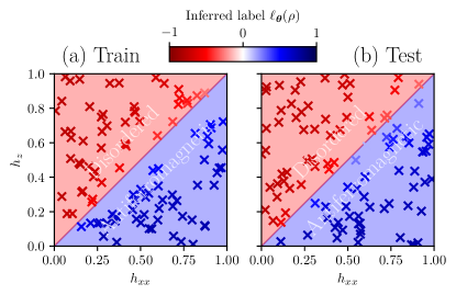
Figure 9: Supervised QML with a classically-efficient circuit. (a) Label assignments from a 50-qubit classifier on a training dataset of disguised TFIM ground states for $T=10$ (details in the main text), across the disordered-antiferromagnetic phase transition. The classifier is trained to minimize the loss function in Eq. (39). (b) Inference on a new set of data drawn from the same distribution. The model achieves 100% classification accuracy on the test dataset.

The quantum classifier is realized as 21 layers of the 2-local ansatz in Eq. (37) (see also Appendix D) and a measurement observable $O=\sigma^{z}_{1}\in i\mathfrak{g}_{0}$. We train it to minimize the loss function in Eq. (39) over the training dataset. Once the parameters trained, we assess accuracy of the classifier on the test dataset. Given trained parameters $\bm{\theta}^{*}$, to perform inference we assign labels as

$$h_{\bm{\theta}^{*}}(\rho_{s})=\operatorname{sgn}(\ell_{\bm{\theta}^{*}}(\rho_{s}))\in\mathcal{Y}\,.$$ (41)

Results are depicted in Fig. 9(a), showing that for this problem the classifier achieves 100% classification accuracy on the new data. Consistent classification accuracy is also verified across multiple random instances of the unitary disguise $V$, thus demonstrating successful application of $\mathfrak{g}{\text{-}}{\rm sim}$ to a supervised QML problem.

We note that in Appendix G, we discuss how the $\mathfrak{g}{\text{-}}{\rm sim}$ phase classifier can be efficiently implemented on a quantum device.

IV Conclusions

Efficient classical simulations of quantum circuits are a valuable tool in scaling towards quantum advantage. In this work, we have presented $\mathfrak{g}$-sim, a classical simulation and optimization framework that relies on the Lie-algebraic structure of the circuits. Reformulating existing results on Lie-algebraic simulation [31, 32] into a modern presentation aimed at the quantum computing community, we further extended these simulation schemes to improve the efficiency of a practical implementation of $\mathfrak{g}{\text{-}}{\rm sim}$. By introducing circuit optimization to this framework, we enabled the scalable classical study of paradigmatic examples relevant for variational quantum computing, demonstrating utility in studying scaling behaviors of VQA problems, improving trainability and mitigating barren plateaus via classical pre-training, and implementing supervised QML problems. These results expand the growing insights in classical pre-training of VQAs [20, 21, 22, 23, 24, 25, 26, 27, 28, 29, 30] and Lie-algebraic study of trainability [42, 43].

Furthermore, we expanded the framework of $\mathfrak{g}{\text{-}}{\rm sim}$ to include compilation and circuit synthesis, which is a novel direction for simulation schemes of this type. By constructing and optimizing a circuit fidelity cost function that can be computed entirely in $\mathfrak{g}{\text{-}}{\rm sim}$, we demonstrated that one can synthesize linear-depth circuits for unitary transformations in $e^{\mathfrak{g}_{0}}$, where $\mathfrak{g}_{0}$ (18) is the algebra used for simulations throughout this work. Compiling such rotations has already proven to be of great utility to the community, with e.g., the use of Givens rotation decomposition to prepare Hartree-Fock states with linear circuit depth [79, 80]. However, our scheme does not necessarily require an underlying free-fermion structure, and therefore expands the class of compilable transformations to include any system corresponding to a $\operatorname{poly}(n)$-dimensional algebra.

To date, Lie-algebraic considerations have been pivotal in many topics of quantum science including quantum error correction [81, 82], controllability of quantum systems [83, 40, 41, 84, 85], efficient measurements [86], dynamical simulations [87, 35], and studying trainability properties of parametrized quantum circuits [42, 43]. Our work has demonstrated further utility in existing applications (dynamical simulations and studying trainability properties), and expanded this list to include classical pre-training of VQAs, efficient circuit compilation, and supervised QML. We anticipate that the $\mathfrak{g}{\text{-}}{\rm sim}$ framework will provide helpful new perspectives and tools in the development of variational quantum computing.

IV.1 Future work

In this work, we have explored a variety of applications of $\mathfrak{g}$-sim. Nonetheless, several applications beyond the scope of this work are apparent.

One of such applications is quantum error mitigation (QEM) [88], a class of techniques which seek to minimize noise-induced biases in quantum algorithm outputs without resorting to full-fledged quantum error correction. In particular, learning-based QEM methods [15, 16, 17, 18] require access to pairs of noisy circuit outputs (obtained from quantum hardware) and corresponding noiseless outputs (obtained from classically-efficient simulation techniques) in order to learn a function mapping noisy outputs to their correct noiseless values. In this context, $\mathfrak{g}{\text{-}}{\rm sim}$ could extend current classical simulation techniques that have been employed.

In a similar vein, $\mathfrak{g}$-sim has potential applications in the context of randomized benchmarking [89]. The greatest limitation in quantum computing is the effect of hardware errors in computations, both coherent and incoherent. There is thus a pressing need to comprehensively characterize the type and magnitude of errors present on quantum hardware. One approach to this is randomized benchmarking, which compares outputs of random gate sequences of increasing length to known expected results without resorting to standard process tomography. Recent work [90] has investigated the use of matchgate circuits for randomized benchmarking. Matchgates are closely related to $\mathfrak{g}_{0}$, and the underlying simulation schemes have much in common with $\mathfrak{g}$-sim. Much like the case of error mitigation, $\mathfrak{g}$-sim could be used to generate benchmarking data for non-matchgate circuits, expanding the scope of these techniques.

We also note the opportunity to further improve the compilation scheme in Sec. III.3. Although its performance appears competitive with the Cartan decomposition approach of Ref. [75], one disadvantage is that our approach requires re-optimization at each time step, whereas the former requires only one optimization. We believe that this limitation could be overcome by using a variational fast-forwarding ansatz [77], which should work since the diagonalization unitary must necessarily be in $\mathcal{G}$. Furthermore, our scheme could trivially be extended to the compilation of evolution unitaries for time-dependent Hamiltonians. In the case of Hamiltonians with periodic Floquet driving, it should even be possible to construct a fast-forwardable solution, which to the best of our knowledge would not be possible with Cartan decomposition methods.

Finally, as discussed earlier and developed further in the Appendices, several generalizations of $\mathfrak{g}{\text{-}}{\rm sim}$ are possible. In particular, while presented here in the context of digital quantum computations, the methodologies can be easily adapted to analog computing. This opens up the possibility of exploring similar applications in this domain, and we anticipate that Lie-algebraic simulations will be valuable for further investigations of the capabilities and constraints of analog and emerging digital-analog quantum platforms [91, 92, 93, 94, 95, 96].

Appendices for “Lie-algebraic classical simulations for variational quantum computing”

Here we present additional details for the main results in our manuscript. The Appendices are organized as follows. First, in Appendix A we present relevant Theorems and their associated proofs. In Appendix B, we describe several techniques that significantly improve the efficiency of our implementation of $\mathfrak{g}{\text{-}}{\rm sim}$. Further expanding these improvements, in Appendix C we present efficient methods for computing gradients to enable optimization of circuits and dynamics with respect to observable cost functions. Then, Appendix D contains the ansatz circuits used throughout the work and further details on the benchmarking procedure used to evaluate the performance of our $\mathfrak{g}{\text{-}}{\rm sim}$ implementation. In Appendix E, we note several algebras of interest closely related to $\mathfrak{g}_{0}$. In Appendix F, we outline some subtleties of unitary compilation with $\mathfrak{g}{\text{-}}{\rm sim}$. Finally, in Appendix G we comment on practical implementation of a $\mathfrak{g}{\text{-}}{\rm sim}$-trained phase classifier on a quantum device.

Appendix A Theorems and proofs

A.1 Representations of unitary evolution

These lemmas follow the approach of Appendix C in Ref. [31].

Lemma 1 (Action of a group operation).

Suppose $U\in\mathcal{G}$ and $\{iG_{\alpha}\}_{\alpha=1}^{\operatorname{dim}(\mathfrak{g})}$ forms a Schmidt-orthonormal basis of $\mathfrak{g}$. Then defining $G^{\prime}_{\alpha}=U^{\dagger}G_{\alpha}U$ for any $G_{\alpha}$, we have $iG^{\prime}_{\alpha}\in\mathfrak{g}$, and thus

$$G^{\prime}_{\alpha}=U^{\dagger}G_{\alpha}U=\sum_{\beta}u_{\alpha\beta}G_{\beta}\,,$$ (42)

with $u_{\alpha\beta}\in\mathbb{C}$.

Proof.

Since $U\in\mathcal{G}$, there exists some $iH\in\mathfrak{g}$ such that $U=e^{-iH}$. The exponential mapping is defined by

$$e^{-iH}=1-iH+\frac{(iH)^{2}}{2!}-\frac{(iH)^{3}}{3!}+\dots\,,$$ (43)

and it follows that

$$G^{\prime}_{\alpha}=G_{\alpha}+i\left[H,G_{\alpha}\right]-\frac{1}{2}\left[H,\left[H,G_{\alpha}\right]\right]+\dots\,.$$ (44)

Since all terms of Eq. (44) are generated by nested commutators of terms of $\mathfrak{g}$ (up to appropriate factors of $i$ for each term), by Definition 1 of the Lie algebra we have that $iG^{\prime}_{\alpha}\in\mathfrak{g}$. ∎

Lemma 2 (Adjoint representation of unitary evolution).

Suppose once again that $U\in\mathcal{G}$, $\{iG_{\alpha}\}_{\alpha=1}^{\operatorname{dim}(\mathfrak{g})}$ forms a Schmidt-orthonormal basis of $\mathfrak{g}$, and consider results of the group operations defined in Eq. (42). Then the corresponding matrix elements $u_{\alpha\beta}$ are those of the adjoint representation of $U$,

$$u_{\alpha\beta}=\left(\Phi^{\operatorname{Ad}}_{\mathcal{G}}(U)\right)_{\alpha\beta}.$$ (45)

Proof.

We again note that since $U\in\mathcal{G}$, there exists some $iH\in\mathfrak{g}$ such that $U=e^{-iH}$. Furthermore, $U$ may be decomposed into infinitesimal steps

$$U=\lim_{M\to\infty}\prod_{m=1}^{M}U^{(\Delta)},$$ (46)

where the infinitesimal unitary is given by

$$U^{(\Delta)}=e^{-i\Delta H}=1-i\Delta H+\mathcal{O}(\Delta^{2})$$ (47)

for $\Delta=1/M$. By Lemma 1 we note that $U^{(\Delta)}$ induces a group operation

$${U^{(\Delta)}}^{\dagger}G_{\alpha}U^{(\Delta)}=\sum_{\beta}(1-v^{(\Delta)}_{\alpha\beta})G_{\beta},$$ (48)

where we have separated out the identity for later convenience without loss of generality. Substituting Equations (47) and (48) into Eq. (44), we obtain

$$G_{\alpha}+i[\Delta H,G_{\alpha}]+\mathcal{O}(\Delta^{2})=G_{\alpha}-\sum_{\beta}v^{(\Delta)}_{\alpha\beta}G_{\beta}.$$ (49)

We may discard vanishing terms in $\mathcal{O}(\Delta^{2})$ since we are in the infinitesimal limit $M\to\infty$. Doing so, and taking $\Tr[G_{\gamma}\dots]$ of both sides of Eq. (49) yields

$$i\Tr[G_{\gamma}[\Delta H,G_{\alpha}]]=-\sum_{\beta}v^{(\delta)}_{\alpha\beta}\Tr[G_{\gamma}G_{\beta}]$$ (50)

$$\implies -\sum_{p}\Delta h_{p}\Tr[G_{\gamma},[G_{p},G_{\alpha}]]=i\Delta v^{(\delta)}_{\alpha\gamma}$$ (51)

$$\implies v^{(\delta)}_{\alpha\gamma}=i\Delta\sum_{k}h_{k}(\bar{\bm{G}}_{k})_{\alpha\gamma}=i\Delta\left(\Phi^{\operatorname{ad}}_{\mathfrak{g}}(H)\right)_{\alpha\gamma},$$ (52)

where we have assumed a basis choice such that the $G_{\alpha}$ are Schmidt-orthonormal (see Definition 6), expanded the adjoint representation, and expanded $H=\sum_{k}h_{k}G_{k}$ for $h_{k}\in\mathbb{R}$. Substituting the result of Eq. (52) into Eq. (48) reveals that the infinitesimal group operation is determined entirely by the adjoint representation $\Phi^{\operatorname{ad}}_{\mathfrak{g}}(H)$

$${U^{(\Delta)}}^{\dagger}G_{\alpha}U^{(\Delta)}=\sum_{\beta}\left(1-i\Delta\Phi^{\operatorname{ad}}_{\mathfrak{g}}(H)\right)_{\alpha\beta}G_{\beta}=\sum_{\beta}\left(e^{-i\Delta\Phi^{\operatorname{ad}}_{\mathfrak{g}}(H)}\right)_{\alpha\beta}G_{\beta}+\mathcal{O}(\Delta^{2}).$$ (53)

We may again discard terms in $\mathcal{O}(\Delta^{2})$ since we are in the infinitesimal limit $M\to\infty$. Noting that the full unitary is obtained by composing infinitesimal steps (Eq. (46)), we obtain from Eq. (53) that

$$U^{\dagger}G_{\alpha}U=\sum_{\beta}\left(e^{-i\Phi^{\operatorname{ad}}_{\mathfrak{g}}(H)}\right)_{\alpha\beta}G_{\beta}=\sum_{\beta}\left(\Phi^{\operatorname{Ad}}_{\mathcal{G}}(U)\right)_{\alpha\beta}G_{\beta},$$ (54)

which is exactly the desired result. ∎

A.2 Evolution of observables under mixed-unitary channels

$\mathfrak{g}{\text{-}}{\rm sim}$ can be easily extended to mixed-unitary channels. Here we state and prove a non-unitary generalization of Result 1, which gives the dynamics of observables under a broader class of processes.

Theorem 3 (Evolution of observables under a mixed-unitary channel in the adjoint representation).

Let $\{G_{1},\dots,G_{\operatorname{dim}(\mathfrak{g})}\}$ be a basis of $\mathfrak{g}$ that admits a faithful adjoint representation, and $\bm{e}^{(\operatorname{in/out})}\in\mathbb{R}^{\operatorname{dim}(\mathfrak{g})}$ be vectors of expectation values of basis observables of $\mathfrak{g}$ such that $\left(\bm{e}^{(\operatorname{in/out})}\right)_{\alpha}\equiv\Tr[G_{\alpha}\rho^{(\operatorname{in/out})}]$. Let $\mathcal{C}:\mathcal{D}(\mathcal{H})\mapsto\mathcal{D}(\mathcal{H})$ be a mixed-unitary channel defined by

$$\mathcal{C}(\rho)\equiv\sum_{m}E_{m}\rho E_{m}^{\dagger},$$ (55)

where the Kraus operators $E_{m}=c_{m}U_{m}$ for $U_{m}\in\mathcal{G}$, $c_{m}\in[0,1]$, $\sum_{m}c_{m}^{2}=1$. Then it follows that

$$\bm{e}^{(\operatorname{out})}=\sum_{m}c_{m}^{2}\bar{\bm{U}}_{m}\bm{e}^{(\operatorname{in})},$$ (56)

where $\bar{\bm{U}}_{m}\equiv\Phi_{\mathfrak{g}}^{\operatorname{Ad}}(U_{m})$, and $\bm{e}^{\operatorname{(in/out)}}$ are computed with respect to evolution under $\mathcal{C}$ as

$$\left(\bm{e}^{(\operatorname{out})}\right)_{\alpha}\equiv\Tr[G_{\alpha}\mathcal{C}(\rho^{(\operatorname{in})})].$$ (57)

Expectation values of observables $O$ with $iO\in\mathfrak{g}$ can be computed by Eq. (12).

Proof.

Taking Eq. (57), expanding the mixed-unitary channel $\mathcal{C}(\rho)\equiv\sum_{m}E_{m}\rho E_{m}^{\dagger}=\sum_{m}c_{m}^{2}U_{m}\rho U_{m}^{\dagger}$ (Eq. (55)), and applying trace linearity and cyclicity, we obtain

$$(\bm{e}^{(\operatorname{out})})_{\alpha} =\Tr[G_{\alpha}\sum_{m}E_{m}\rho^{(\operatorname{in})}E_{m}^{\dagger}]$$ (58)

$$=\sum_{m}c_{m}^{2}\Tr[U_{m}^{\dagger}G_{\alpha}U_{m}\rho^{(\operatorname{in})}].$$ (59)

Applying Lemma 45 and simplifying, we obtain

$$(\bm{e}^{(\operatorname{out})})_{\alpha} =\sum_{m}c_{m}^{2}\Tr[\sum_{\beta}\left(\Phi^{\operatorname{Ad}}_{\mathcal{G}}(U_{m})\right)_{\alpha\beta}G_{\beta}\rho^{(\operatorname{in})}]$$ (60)

$$=\sum_{m}c_{m}^{2}\sum_{\beta}\left(\Phi^{\operatorname{Ad}}_{\mathcal{G}}(U_{m})\right)_{\alpha\beta}(\bm{e}^{(\operatorname{in})})_{\beta},$$ (61)

which is simply Eq. (56) in index form. ∎

A.3 Evolution of correlators under mixed-unitary channels

Evolution of correlators can also be generalized to mixed-unitary channels. Here we state and prove a more general version of Result 16.

Theorem 4 (Evolution of correlators under a mixed-unitary channel in the adjoint representation).

Consider evolution under a mixed-unitary channel $\rho^{(\operatorname{out})}=\mathcal{C}(\rho^{(\operatorname{in})})$ as defined in Theorem 3, and initial/final correlators $\bm{E}^{(\operatorname{in/out})}$ as defined in Eq. (14). Then, it follows that

$$\bm{E}^{(\operatorname{out})}=\sum_{m}c_{m}^{2}\bar{\bm{U}}_{m}\bm{E}^{(\operatorname{in})}\bar{\bm{U}}_{m}^{T},$$ (62)

Furthermore, suppose $iO^{(a)},iO^{(b)}\in\mathfrak{g}$ such that $O^{(a)}=\sum_{\alpha}(\bm{w}^{(a)})_{\alpha}G_{\alpha}$, $O^{(b)}=\sum_{\alpha}(\bm{w}^{(b)})_{\alpha}G_{\alpha}$. Then the latter value of the correlator $\langle O^{(a)}O^{(b)}\rangle$ may be computed as

$$\Tr[O^{(a)}O^{(b)}\rho^{(\operatorname{out})}]={\bm{w}^{(a)}}^{T}\bm{E}^{(\operatorname{out})}\bm{w}^{(b)}.$$ (63)

Proof.

We seek to compute expectation values of all $\langle G_{\alpha}G_{\beta}\rangle$ for the state $\rho^{(out)}$. These are given by

$$\left(\bar{\bm{e}}^{(\operatorname{out})}\right)_{\alpha\beta}\equiv\Tr[G_{\alpha}G_{\beta}\rho^{(\operatorname{out})}]=\Tr[G_{\alpha}G_{\beta}\mathcal{C}(\rho^{(\operatorname{in})})]=\sum_{m}c_{m}^{2}\Tr[U_{m}^{\dagger}G_{\alpha}U_{m}U_{m}^{\dagger}G_{\beta}U_{m}\rho^{(\operatorname{in})}],$$ (64)

where we have expanded the mixed-unitary channel $\mathcal{C}$, used trace properties, and inserted the identity $U_{m}U_{m}^{\dagger}=1$ in the last step. Noting that $G_{\alpha}$ and $G_{\beta}$ are transformed by group operations and applying Lemma 45, we obtain

$$\bar{\bm{e}}^{(\operatorname{out})}=\sum_{m,\alpha^{\prime},\beta^{\prime}}c_{m}^{2}\left(\Phi^{\operatorname{Ad}}_{\mathcal{G}}(U_{m})\right)_{\alpha,\alpha^{\prime}}\left(\Phi^{\operatorname{Ad}}_{\mathcal{G}}(U_{m})\right)_{\beta,\beta^{\prime}}\Tr[G_{\alpha^{\prime}}G_{\beta^{\prime}}\rho^{(\operatorname{in})}],$$ (65)

which is Eq. (16) in index form, proving the former part of the theorem. The latter part of the theorem follows trivially by taking the left-hand side of Eq. (63), expanding $O^{(a/b)}=\sum_{j}(\bm{w}^{(a/b)})_{\alpha}G_{\alpha}$, and identifying matrix operations in index form. ∎

A.4 Higher-order correlators

We can further generalize Theorem 63 to higher-order correlators. The complexity of computing an $M$th order correlator is naïvely $\mathcal{O}(\operatorname{dim}(\mathfrak{g})^{2M})$ as discussed in the following remark.

Remark 1 (Generalization to higher-order correlators).

By following the approach of Sec. A.3 (taking the correlator expectation value, expanding the channel, using trace cyclicity and inserting identities, applying Lemma 45), these results generalize straightforwardly to $M$th order correlators $\langle G_{\alpha_{1}}\dots G_{\alpha_{M}}\rangle$. The evolution requires contraction of an $M$-th order tensor as depicted in Fig. 10, which is naïvely $\mathcal{O}(\operatorname{dim}(\mathfrak{g})^{2M})$. Thus, despite being classically efficient up to fixed $M$, computing high-order correlators quickly becomes impractical as $M$ increases. For the purposes of the current work, we only require $M\leqslant 2$.

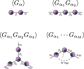
Figure 10: Tensor contractions for $\mathfrak{g}$-sim evolution. Tensor diagrams for the contractions required for computing dynamics with $\mathfrak{g}{\text{-}}{\rm sim}$ at first order $\langle G_{\alpha}\rangle$, second order $\langle G_{\alpha_{1}}G_{\alpha_{2}}\rangle$, third order $\langle G_{\alpha_{1}}G_{\alpha_{2}}G_{\alpha_{3}}\rangle$, and arbitrary $M$-th order $\langle G_{\alpha_{1}}\dots G_{\alpha_{M}}\rangle$.

We note that for certain initial states, the evaluation of higher-order correlators can be simplified. Given an initial generalized coherent state, one may factorize the $M$-th order correlator $\langle G_{i_{1}}\dots G_{i_{M}}\rangle$ using Wick’s theorem, resulting in a highly simplified matrix product form for the correlator tensor that can be evaluated more efficiently. Such a method is outlined in Appendix F of Ref. [31].

A.5 Analog computing

So far, we have only considered the evolution of states under the action of quantum circuits (or corresponding mixed-unitary channels). Still, the principles underpinning $\mathfrak{g}{\text{-}}{\rm sim}$ can equally be applied to the case where the system is continuously driven (i.e., in the analog computing paradigm).

In the following, we consider evolution under a time-dependent Hamiltonian

$$\mathcal{H}(t)=\sum_{h}c_{h}(t)H_{h},$$ (66)

with constituents $iH_{h}\in\mathfrak{g}$ and control functions $c_{h}(t)$. Given an initial state $\rho^{(in)}$, the state of the system at time $t$ can be expressed as $\rho(t)=U(t)\rho^{(in)}U^{\dagger}(t)$ where $U(t)=\mathcal{T}\big{[}{\rm exp}(-i\int^{t}_{0}\,\mathcal{H}(t^{\prime})\,dt^{\prime})\big{]}$ with $\mathcal{T}$ the time-ordering operator. In analogy to simulation in the quantum circuit scenario, we are now tasked with evaluating the expectation value $\langle O\rangle\equiv{\rm Tr}[O\rho(T)]$ of an observable $O$ supported by $\mathfrak{g}$ for the state $\rho(t=T)$ obtained at the end of the evolution.

Defining (in the Heisenberg picture) the time-dependent operator $O(t)\equiv U^{\dagger}(t)OU(t)$, we have that $\langle O\rangle={\rm Tr}[O(T)\rho^{(\operatorname{in})}]$. Furthermore, the time evolution of $O(t)$ satisfies the ordinary differential equation (ODE):

$$\frac{d}{dt}O(t)=i[\mathcal{H}(t),O(t)],$$ (67)

with initial condition $O(t=0)=O$. From the Definition. 6 of the adjoint representation and the definition of the structure constants in Eq. (5), it can be verified that

$$[\mathcal{H}(t),G_{\alpha}]=\sum_{\beta}\big{[}\Phi_{\mathfrak{g}}^{\operatorname{ad}}(\mathcal{H}(t))\big{]}_{\alpha\beta}G_{\beta},$$ (68)

with the matrix $\Phi_{\mathfrak{g}}^{\operatorname{ad}}(\mathcal{H}(t))=\sum_{h}c_{h}(t)\Phi_{\mathfrak{g}}^{\operatorname{ad}}(H_{h})$.

Hence, decomposing $O(t)=\sum_{\alpha}(\mathbf{o}(t))_{\alpha}G_{\alpha}$ in the observable basis $\{G_{\alpha}\}$ of $\mathfrak{g}$, one can recast Eq. (67) as the ODE

$$\frac{d}{dt}\mathbf{o}(t)=i\Phi_{\mathfrak{g}}^{\operatorname{ad}}(\mathcal{H})\mathbf{o}(t)$$ (69)

over the vector $\mathbf{o}(t)$.

In summary, evaluating the expectation value $\langle O\rangle$ consists in two steps. First, solve the dynamics of $\mathbf{o}(t)$ from $t=0$ to $t=T$ according to Eq. (69). This is achieved by standard numerical ODE solvers, and only requires acting on a $\operatorname{dim}(\mathfrak{g})$ vector space. Then, upon evaluation of $\mathbf{o}(T)$, one can compute $\langle O\rangle=\mathbf{o}(T)\cdot\mathbf{e}^{(\operatorname{in})}$, where we recall that the vector $\bm{e}^{(\operatorname{in})}$ contains the expectation values $\Tr[G_{\alpha}\rho^{(\operatorname{in})}]$ of all $G_{\alpha}$ with respect to the initial state.

Overall, this extends the scope of $\mathfrak{g}{\text{-}}{\rm sim}$ to analog (and digital-analog) quantum computing scenarios. As an example of application, in Ref. [98] such capabilities were used to evaluate (and optimize) continuous diabatic schedules for tasks of ground state preparations over system sizes of up to $n=39$ spins.

Appendix B Efficient implementation of $\mathfrak{g}{\text{-}}{\rm sim}$

The $\mathfrak{g}{\text{-}}{\rm sim}$ framework outlined in Section II.3 allows scalable classical simulations for observables supported by $\mathfrak{g}$ whenever $\operatorname{dim}(\mathfrak{g})\in\mathcal{O}(\operatorname{poly}(n))$. Although these techniques are known [31, 32], one contribution of this work is to introduce new optimizations which substantially improve the efficiency of $\mathfrak{g}{\text{-}}{\rm sim}$. In the following subsections, we detail three main improvements:

• Pre-computing eigendecompositions of gate generator adjoint representations reduces the time complexity of $\mathfrak{g}{\text{-}}{\rm sim}$ evolution from $\mathcal{O}(\operatorname{dim}(\mathfrak{g})^{3})$ to $\mathcal{O}(\operatorname{dim}(\mathfrak{g})^{2})$ (B.1).

• Relevant matrices are extremely sparse when $\mathfrak{g}$ has a Pauli basis, allowing speedups by use of sparse methods, even for subalgebras whose generators are not sparse (B.2).

• Eigendecompositions of gates with Pauli generators can be computed in $\mathcal{O}(\operatorname{dim}(\mathfrak{g}))$ in the representation of a Pauli basis, instead of the usual $\mathcal{O}(\operatorname{dim}(\mathfrak{g})^{3})$ (B.3).

In practice, we found such optimizations to significantly accelerate our simulations, and all the numerics presented in this work rely on a Python implementation of $\mathfrak{g}{\text{-}}{\rm sim}$ incorporating them.

B.1 Efficient evolution

Evaluating each of the $LK$ terms $e^{-i\theta\bar{\bm{H}}_{k}}$ appearing in Eq. (13) of the simulation routine has time complexity scaling as $\mathcal{O}(\operatorname{dim}(\mathfrak{g})^{3})$ using standard matrix exponentiation routines. However, given the full-rank eigendecompositions

$$\bar{\bm{H}}_{k}=\bar{\bm{Q}}_{k}\text{diag}(\epsilon_{k}^{(1)},\ldots,\epsilon_{k}^{(\operatorname{dim}(\mathfrak{g}))})\bar{\bm{Q}}_{k}^{T}$$ (70)

of the (adjoint representation of the) gate generators $\bar{\bm{H}}_{k}$, the action of these parametrized gates is given as

$$\Phi_{\mathcal{G}}^{\operatorname{Ad}}(e^{-i\theta H_{k})}=\bar{\bm{Q}}_{k}\text{diag}(e^{-i\theta\epsilon_{k}^{(1)}},\dots,e^{-i\theta\epsilon_{k}^{(\operatorname{dim}(\mathfrak{g}))}})\bar{\bm{Q}}_{k}^{T},$$ (71)

which can be applied to a vector $\bm{e}\in\mathbb{R}^{\operatorname{dim}(\mathfrak{g})}$ with $\mathcal{O}(\operatorname{dim}(\mathfrak{g})^{2})$ time complexity. Notably, these decompositions only need to be performed once per algebra and per gate generator used, the number of which is typically no more than linear in the system size $n$. Pre-computing these eigendecompositions naïvely scales as $\mathcal{O}(\operatorname{dim}(\mathfrak{g})^{3})$, however, in Appendix B.3 we detail a procedure by which the eigendecompositions for $\mathfrak{g}_{0}$ can be computed in $\mathcal{O}(\operatorname{dim}(\mathfrak{g}))$. An explicit algorithm for simulation incorporating these pre-computed eigendecompositions is provided in Algorithm 1.

Algorithm 1 Efficient evolution of observable expectation values using $\mathfrak{g}$-sim.

Circuit parameters $\bm{\theta}$, input observables $\bm{e}^{(\text{in})}$, circuit generator eigendecompositions (Eq. (71)) $\bar{\bm{Q}}_{k}$ and $\epsilon_{k}^{(g)}$

$\bm{e}^{(\operatorname{out})}\leftarrow\bm{e}^{(\text{in})}$

for $l$ in $1,\dots,L$ do

     for $m$ in $1,\dots,M$ do

         $\bm{e}^{(\operatorname{out})}\leftarrow\bar{\bm{Q}}_{k}^{T}\bm{e}^{(\operatorname{out})}$

         for $g$ in $1,\dots,\text{dim}(\mathfrak{g})$ do

              $(\bm{e}^{(\operatorname{out})})_{g}\leftarrow e^{-i\theta_{lk}\epsilon_{k}^{(g)}}(\bm{e}^{(\operatorname{out})})_{g}$

         end for

         $\bm{e}^{(\operatorname{out})}\leftarrow\bar{\bm{Q}}_{k}\bm{e}^{(\operatorname{out})}$

     end for

end for

Vector $\bm{e}^{(\operatorname{out})}$ of basis observables in $\mathfrak{g}$

$\mathcal{O}(M\operatorname{dim}(\mathfrak{g})^{2})$

B.2 Sparsity of adjoint representation

When the relevant basis of $\mathfrak{g}$ consists of Pauli strings and the gate generators are also Pauli strings (e.g. when performing simulations in $\mathfrak{g}_{0}$ where all gates have Pauli operator generators), the adjoint representations $\bar{\bm{H}}_{l}$ of the gate generators and their corresponding parametrized gates are of an extremely sparse form, having fewer than $2\operatorname{dim}(\mathfrak{g})$ nonzero entries per $(\operatorname{dim}(\mathfrak{g})\times\operatorname{dim}(\mathfrak{g}))$-dimensional matrix. Thus, substantial speedups can be obtained by leveraging sparse linear algebra libraries. This is the case for most simulations presented in this work.

However, we sometimes must apply gates whose generators are not Pauli strings, such as $e^{-i\theta\sum_{j=1}^{n-1}\sigma^{x}_{j}\sigma^{x}_{j+1}}$ for VQE on the LTFIM (Sec. III.2.2), or $e^{-i\theta\sum_{j=1}^{n-1}\sigma^{z}_{j}\sigma^{z}_{j+1}}$ for QAOA (Sec. III.2.3). For gates like these, the adjoint representation of the generator does not admit an efficient sparse representation, and will in general be dense. Figure 11 depicts this difference in sparsity.

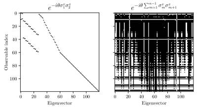
Figure 11: Sparsity of gates generated by Pauli strings versus general gates. We plot sparsity maps for the eigenvector matrix $\bar{\bm{Q}}$ where $\Phi_{\mathcal{G}}^{\operatorname{Ad}}(\exp(-i\theta H))=\bar{\bm{Q}}\text{diag}(e^{-i\theta\epsilon^{(1)}},\dots,e^{-i\theta\epsilon^{(\operatorname{dim}(\mathfrak{g}))}})\bar{\bm{Q}}^{T}$, for $H=\sigma^{x}_{1}\sigma^{x}_{2}$ (left) and $H=\sum_{m=1}^{n-1}\sigma^{x}_{m}\sigma^{x}_{m+1}$ (right), for a system of $n=8$ qubits. White (black) entries in the map indicates (non) zero entries. The gate $\exp(-i\theta\sigma^{x}_{1}\sigma^{x}_{2})$ has a sparse eigenvector matrix since it is generated by a single Pauli string, whereas the gate $\exp(-i\theta\sum_{m=1}^{n}\sigma^{x}_{m}\sigma^{x}_{m+1})$ has a dense eigenvector matrix since it is generated by a sum of Pauli strings.

For gates not generated by single Pauli strings, but rather sums of commuting Pauli strings, one can factorize the gate and still use sparse methods. For example

$$e^{-i\theta\sum_{j=1}^{n-1}\sigma^{x}_{j}\sigma^{x}_{j+1}} =\prod_{j=1}^{n-1}e^{-i\theta\sigma^{x}_{j}\sigma^{x}_{j+1}}$$ (72)

$$\implies\underbrace{\Phi_{\mathcal{G}}^{\operatorname{Ad}}\left(e^{-i\theta\sum_{j=1}^{n-1}\sigma^{x}_{j}\sigma^{x}_{j+1}}\right)}_{\text{dense}} =\prod_{j=1}^{n-1}e^{-i\theta\overbrace{\Phi_{\mathfrak{g}}^{\operatorname{ad}}(\sigma^{x}_{j}\sigma^{x}_{j+1})}^{\text{sparse}}},$$ (73)

since the adjoint representation is a Lie algebra homomorphism. However, in such cases the dense nature of the eigenvector matrix can make GPU-accelerated dense linear algebra methods highly appealing. For example, we consider tests on our hardware (a single core of an Intel Xeon Platinum 8268 for CPU methods vs a NVIDIA Tesla V100 for GPU methods), for our implementation of $\mathfrak{g}$-sim. We found that for systems with sparse gates only, GPU acceleration provided an overall speedup of a factor of 3-5 versus a single CPU core, whereas for systems with dense gates, GPU acceleration provided an overall speedup of a factor of 60-100. The choice of sparse or dense methods and CPU or GPU hardware must be made judiciously depending on problem type and the need for parallelizability.

B.3 Efficient calculation and eigendecomposition of Pauli-basis adjoint representations

For our Lie-algebraic simulations, we must be able to compute the adjoint representations (Definition 6) of our gate generators $H_{k}$:

$$\left(\bar{\bm{H}}_{k}\right)_{\alpha\beta}=-\Tr\left[H_{k}\left[G_{\alpha},G_{\beta}\right]\right].$$ (74)

naïvely computing an adjoint representation via Eq. (74) would scale as $\mathcal{O}(\operatorname{dim}(\mathfrak{g})^{2})$. However, if the basis operators $G_{\alpha}$ of $\mathfrak{g}$ are Pauli strings

$$G_{\alpha}=\bigotimes_{m=1}^{n}\sigma_{m}^{s_{\alpha,m}},\quad s_{\alpha,m}\in\{x,y,z\},$$ (75)

as is the case for $\mathfrak{g}_{0}$, and $H_{k}$ is also a Pauli string, then for fixed $k$ and $\alpha$ ($\beta$), Eq. (74) has a nonzero value for at most one value of $\beta$ ($\alpha$). That is, each row and column have at most one nonzero entry. Thus, one can construct the adjoint representation for $\bar{\bm{H}}_{k}$ in just $\mathcal{O}(\operatorname{dim}(\mathfrak{g}))$ by iterating over $\alpha\in\{1,\dots,\operatorname{dim}(\mathfrak{g})\}$, inverting Eq. (74) to find the Pauli string $\sigma$ such that $\Tr[H_{k}[G_{\alpha},\sigma]]$ (which is possible since $H_{k}$ and $G_{\alpha}$ are Pauli strings), checking if $\sigma=G_{\beta}$ for some $\beta$ (which can be done in $\mathcal{O}(n)$ by using a hashmap), and populating the corresponding element if so.

Similarly, although naïvely computing the eigendecomposition (70) would be $\mathcal{O}(\operatorname{dim}(\mathfrak{g})^{3})$, one may compute it in just $\mathcal{O}(\operatorname{dim}(\mathfrak{g}))$ in the case where the $H_{k}$ and $G_{\alpha}$ are Pauli strings. Since the $\bar{\bm{H}}_{k}$ are Hermitian and at most one element of each row/column is nonzero, the adjoint representations take the form (up to some permutation of rows and columns)

$$\bar{\bm{H}}_{k}=2\left(\bigoplus_{m_{1}=1}^{(\operatorname{dim}(\mathfrak{g})-\operatorname{dim}(\ker(\bar{\bm{H}}_{k})))/2}\bar{\bm{\sigma}}^{y}\right)\oplus\left(\bigoplus_{m_{2}=1}^{\operatorname{dim}(\ker(\bar{\bm{H}}_{k}))/2}\bar{\bm{0}}\right),$$ (76)

where the factor of $2$ originates from the Pauli commutation relations, and $\bar{\bm{\sigma}}^{y}=\begin{bmatrix}0&-i\\ i&0\end{bmatrix}$ and $\bar{\bm{0}}=\begin{bmatrix}0&0\\ 0&0\end{bmatrix}$ are the Pauli Y matrix and the zero matrix, respectively. Since the eigendecomposition of $\bar{\bm{\sigma}}^{y}$ is known, one may compute the eigendecomposition of $\bar{\bm{H}}_{k}$ in $\mathcal{O}(\operatorname{dim}(\mathfrak{g}))$ by iterating over the $\bar{\bm{\sigma}}_{y}$ summands, populating the corresponding eigenvectors and eigenvalues, and using any set of vectors spanning $\ker(\bar{\bm{H}}_{k})$ as the remaining eigenvectors with zero eigenvalues.

Appendix C Gradient calculations

C.1 Observable gradients

For VQA and QML applications, it is often beneficial to be able to efficiently calculate gradients $\gradient_{\bm{\theta}}\langle O\rangle$ of observables $O=\sum_{\alpha}(\bm{w})_{\alpha}G_{\alpha}$ for $\bm{w}\in\mathbb{R}^{\operatorname{dim}(\mathfrak{g})}$, $iG_{\alpha}\in\mathfrak{g}$. Differentiating Eq. (12) with respect to $\theta_{m}$, we find

$$(\gradient_{\bm{\theta}}\langle O\rangle)_{m}=\frac{\partial\langle O\rangle}{\partial\theta_{m}}=\bar{\bm{w}}^{T}\left(\frac{\partial\Phi^{\operatorname{Ad}}_{\mathcal{G}}(U(\bm{\theta}))}{\partial\theta_{m}}\right)\bar{\bm{e}}^{(\text{in})},$$ (77)

where we may compute

$$\frac{\partial\Phi^{\operatorname{Ad}}_{\mathcal{G}}(U(\bm{\theta}))}{\partial\theta_{m}}=-i\left(\bar{\bm{U}}_{m+1:M}\bar{\bm{H}}_{k}\bar{\bm{U}}_{1:m}\right),$$ (78)

where $\bar{\bm{U}}_{a:b}\equiv e^{-i\theta_{b}\bar{\bm{H}}_{b}}e^{-i\theta_{b-1}\bar{\bm{H}}_{b-1}}\dots e^{-i\theta_{a}\bar{\bm{H}}_{a}}$, $m$ is a combined index for $l$ and $k$, and $M=LK$. Naïvely evaluating Eq. (78) requires $\mathcal{O}(M^{2})$ matrix-vector multiplications (each $\mathcal{O}(\operatorname{dim}(\mathfrak{g})^{2})$), however by exploiting a recurrent property of the gradients, one may compute the gradient with only $\mathcal{O}(M)$ matrix-vector multiplications (i.e., with the same asymptotic complexity as simulating the circuit in the first place). This procedure, which follows the ‘reverse-mode’ gradient calculation of Ref. [44] in conjunction with the efficient spectral approach of Algorithm 1, is outlined in Algorithm 2.

Algorithm 2 Calculating gradients in $\mathfrak{g}$-sim.

Circuit $\bm{\theta}$, input expectation value vector $\bm{e}^{(\text{in})}$, circuit generator adjoint representations $\bar{\bm{H}}_{k}$ and eigendecompositions $\bar{\bm{Q}}_{k}$, $\epsilon_{k}^{(g)}$, coefficients $\bm{w}$ of observable $O$

$\bm{\lambda}\leftarrow\bar{\bm{U}}\bm{e}^{(\text{in})}$ $\triangleright$ Use the main loop of Algorithm 1.

$\bm{\phi}\leftarrow\bm{w}$

$(\gradient_{\bm{\theta}}\langle O\rangle)_{M}\leftarrow-i\bm{\phi}^{T}\bar{\bm{H}}_{M}\bm{\lambda}$

for $m$ in $N,\dots,2$ do

     $\bm{\lambda}\leftarrow\bar{\bm{Q}}_{m}\bm{\lambda}$

     $\bm{\phi}\leftarrow\bar{\bm{Q}}_{m}\bm{\phi}$

     for $g$ in $1,\dots,\operatorname{dim}(\mathfrak{g})$ do

         $\lambda_{g}\leftarrow e^{i\theta_{m}\epsilon_{m}^{(g)}}\lambda_{g}$

         $\phi_{g}\leftarrow e^{i\theta_{m}\epsilon_{m}^{(g)}}\phi_{g}$

     end for

     $\bm{\lambda}\leftarrow\bar{\bm{Q}}_{m}^{T}\bm{\lambda}$

     $\bm{\phi}\leftarrow\bar{\bm{Q}}_{m}^{T}\bm{\phi}$

     $(\gradient_{\bm{\theta}}\langle O\rangle)_{m-1}\leftarrow-i\bm{\phi}^{T}\bar{\bm{H}}_{m}\bm{\lambda}$

end for

Gradient vector $\gradient_{\bm{\theta}}\langle O\rangle$

$\mathcal{O}(M\operatorname{dim}(\mathfrak{g})^{2})$

Higher order derivatives can also be computed, such as the Hessian

$$(\gradient_{\bm{\theta}}^{2}\langle O\rangle)_{jk}=\frac{\partial^{2}\langle O\rangle}{\partial\theta_{j}\partial\theta_{k}}=-\bar{\bm{h}}^{T}\bar{\bm{U}}_{k+1:N}\bar{\bm{H}}_{k}\bar{\bm{U}}_{j:k}\bar{\bm{H}}_{j}\bar{\bm{U}}_{1:j}\bar{\bm{e}}^{(\text{in})}.$$ (79)

However, since the circuit generators $\bar{\bm{H}}_{k}$ are typically non-invertible, Algorithm 2 cannot be generalized to evaluate Eq. (79) and higher-order derivatives. Although still polynomial in complexity, evaluating a $P$-th order gradient for $P\geqslant 2$ will be a factor $\mathcal{O}(M^{P})$ slower than efficiently evaluating the gradient.

C.2 Compilation cost function gradients

For unitary compilation (Sec. III.3), the use of gradient-based optimizers requires the efficient calculation of $\partial\mathcal{L}_{\mathfrak{g}}/\partial\theta_{m}$. Differentiating Eq. (35), we obtain

$$\frac{\partial\mathcal{L}_{\mathfrak{g}}}{\partial\theta_{m}}=\frac{1}{\operatorname{dim}(\mathfrak{g})}\operatorname{Im}\left[\Tr[\bar{\bm{V}}^{T}\bar{\bm{U}}_{m+1:M}\bar{\bm{H}}_{m}\bar{\bm{U}}_{1:m}]\right],$$ (80)

where we have used properties of the ansatz structure, given in Eq. (1), and $\bar{\bm{U}}^{T}_{n:m}\equiv\bar{\bm{U}}^{T}_{n}\bar{\bm{U}}^{T}_{n+1}\dots\bar{\bm{U}}^{T}_{m}$. Noting that the matrix terms in Eq. (80) have the same recurrent form as Eq. (78), we may compute the full gradient vector in $\mathcal{O}(N\operatorname{dim}(\mathfrak{g})^{3})$ by a straightforward modification of Algorithm 2 (with matrix-matrix multiplication instead of matrix-vector multiplication).

For efficient implementation, care should be taken with the order of operations when evaluating Eqs. (35) and (80), in particular to avoid any dense-dense matrix multiplication. For example, in Eq. (80), one should store the products $(\bar{\bm{U}}_{m+1:m})^{T}\bar{\bm{V}}$ and $\bar{\bm{U}}_{1:m}$ as dense matrices, use sparse representations of the $\bar{\bm{U}}_{m}$ when applying the iterative step in Algorithm 2, and use sparse representations of $\bar{\bm{H}}_{m}$ when evaluating each element of the gradient. We find that with this order of operations, the evaluation is substantially accelerated by the use of sparse-dense matrix multiplication algorithms, and further improved by the use of GPU acceleration (e.g. SpDM with cuSPARSE). Finally, the trace in Eq. (80) of the product of two dense matrices ($\bar{\bm{V}}^{T}\bar{\bm{U}}_{m+1:M}$ and $\bar{\bm{H}}_{m}\bar{\bm{U}}_{1:m}$) can be evaluated in a dense $\mathcal{O}(\operatorname{dim}(\mathfrak{g})^{2})$ operation as

$$\Tr[\bar{\bm{V}}^{T}\bar{\bm{U}}_{m+1:M}\bar{\bm{H}}_{m}\bar{\bm{U}}_{1:m}]=\sum_{\alpha\beta}\left[((\bar{\bm{U}}_{m+1:m})^{T}\bar{\bm{V}})\circ(\bar{\bm{H}}_{m}\bar{\bm{U}}_{1:m})\right]_{\alpha\beta},$$ (81)

where $\circ$ denotes the Hadamard product. This avoids costly $\mathcal{O}(\operatorname{dim}(\mathfrak{g})^{3})$ dense-dense matrix multiplication entirely, which would otherwise be by far the most expensive operation in this procedure.

C.3 Analog computing

Gradients of expectation values can also be obtained in the analog computing scenario that was laid out in Appendix A.5. While not providing full-fledged details of the implementation required, we specify the problem and point the reader toward dedicated references for implementation.

In the analog computing scenario, control of the system occurs at the Hamiltonian level through the control functions $c_{h}(t)$ appearing in Eq. (66). A first step towards defining the gradients of interest requires parametrizing these control functions in terms of a finite set of parameters $\bm{\theta}$ (i.e., $c_{h}(t)\rightarrow c_{h}(\bm{\theta},t)$). Upon such parametrization, and given an observable $O$, an optimization task would consist in identifying values of $\bm{\theta}$ that minimize the expectation value $\langle O\rangle$, with the gradients of interests denoted $\partial\langle O\rangle/\partial_{\bm{\theta}_{m}}$.

While similar in notations to the gradients of the circuit parameters in Eq. (77), we note that depending on the parametrization of the controls adopted, each of the control parameter may affect the control values along the whole evolution, and would appear particularly difficult to evaluate. Still, progress have been made towards efficient evaluation of such gradients in the context of quantum optimal control and machine learning. In particular, methods presented in Refs. [99, 100] generically enable such calculations and require to numerical solve an augmented ODE, but avoid the necessity of storing in memory the state of the system along each numerical step of its evolution. Applications of these numerical methods have already found application in quantum optimal control problems [101, 102] but to-date have remained limited to small system sizes due to the exponentially growth of the underlying Hilbert space. Incorporating them with $\mathfrak{g}{\text{-}}{\rm sim}$ would circumvent such limitations for certain quantum dynamics.

Appendix D Ansatz circuits and benchmarking

Details of all ansatz circuits used in this work are given in Table 1.

D.1 Benchmark calculations

For the compute time benchmarks in Fig. 2, we repeatedly simulate evolution of a state initialized to $\ket{\bm{0}}$ and transformed by a single layer ($L=1$) of the TFXY 2-local ansatz (see Table 1) using both our Python implementation of $\mathfrak{g}{\text{-}}{\rm sim}$ and TensorFlow Quantum on a single core of an Intel Xeon Platinum 8268. We stress that unlike tensor network methods, the time complexity of applying a gate is independent of circuit depth, so we report our timings per gate. We collect timings using the timeit Python package in batches of repeated simulations (to minimize the influence of measurement distortion due to environmental factors) and average over batches. We bootstrap 95% confidence intervals on these averages, but they are too small to be visualized in Fig. 2.

Memory requirements for state vectors are computed assuming double-precision arithmetic on a $2^{n}$-dimensional Hilbert space $\mathcal{H}$. Memory requirements for $\mathfrak{g}{\text{-}}{\rm sim}$ are computed by profiling the actual memory footprint of the observable vector $\bm{e}$ and algebra data (adjoint representations of generators $\bar{\bm{H}}_{k}$ and their eigendecompositions).

\begin{overpic}[abs,unit=1mm,width=433.62pt]{figures/ansatze.pdf} \put(7.0,48.0){\parbox{144.54pt}{ Benchmarking (\ref{sec:efficient_implementation_gsim}) \\ TFXY VQE (\ref{sec:overparametrization}) \\ Random compilation (\ref{sec:compilation_random}) \\ Phase classifier (\ref{sec:supervised_QML}) \vspace{0.45in} \\ Dynamics compilation (\ref{sec:compiling_dynamics}) \vspace{0.55in} \\ LTFIM pre-training (\ref{sec:LTFIM}) \vspace{0.4in} \\ LTFIM pre-training (\ref{sec:LTFIM}) \vspace{0.4in} \\ QAOA pre-training (\ref{sec:QAOA}) \vspace{0.45in} \\ QAOA pre-training (\ref{sec:QAOA}) } } \end{overpic}

Table 1: Layers of all variational ansätze used in this work, with reference to their applications, whether or not they are classically efficient in $\mathfrak{g}{\text{-}}{\rm sim}$ (for simulating dynamics of observables supported by $\mathfrak{g}$), and circuit diagrams for single layers of each ansatz. In diagrams where individual qubits are depicted, the example layer is given for $n=3$ for compactness.

Appendix E Subalgebras of $\mathfrak{g}_{0}$

Throughout this work, we use the algebra $\mathfrak{g}_{0}$, defined in Eq. (18), which has dimension $\operatorname{dim}(\mathfrak{g}_{0})=n(2n-1)$ and encompasses many models of interest:

• The Hamiltonian algebra for the XY model with open boundary conditions and free coefficients forms a proper subalgebra $\mathfrak{g}_{\text{XY}}\subset\mathfrak{g}_{0}$ with $\text{dim}(\mathfrak{g}_{\text{XY}})=n(n-1)$ [75], given by

  $$\mathfrak{g}_{\text{XY}}={\rm span}_{\mathbb{R}}\left\langle\left(\{i\sigma^{x}_{j}\sigma^{x}_{j+1}\}_{j=1}^{n-1}\right)\cup\left(\{i\sigma^{y}_{j}\sigma^{y}_{j+1}\}_{j=1}^{n-1}\right)\right\rangle_{\operatorname{Lie}}.$$ (82)

• The Hamiltonian algebra for the transverse field Ising model (TFIM) with open boundary conditions and non-free coupling coefficients forms a proper subalgebra $\mathfrak{g}_{\text{TFIM}}\subset\mathfrak{g}_{0}$ with $\text{dim}(\mathfrak{g}_{\text{TFIM}})=n^{2}$ [47], given by

  $$\mathfrak{g}_{\text{TFIM}}={\rm span}_{\mathbb{R}}\left\langle\left(i\sum_{j=1}^{n-1}\sigma^{x}_{j}\sigma^{x}_{j+1}\right)\cup\left(i\sum_{j=1}^{n}\sigma^{z}_{j}\right)\right\rangle_{\operatorname{Lie}}.$$ (83)

• For a path graph $P_{n}$ on n vertices, the circuit of the quantum approximate optimization algorithm [65] has an associated algebra

  $$\mathfrak{g}_{\text{QAOA,}P_{n}}={\rm span}_{\mathbb{R}}\left\langle\left(i\sum_{j=1}^{n-1}\sigma^{z}_{j}\sigma^{z}_{j+1}\right)\cup\left(i\sum_{j=1}^{n}\sigma^{x}_{j}\right)\right\rangle_{\operatorname{Lie}},$$ (84)

  which is isomorphic to the one of the TFIM, $\mathfrak{g}_{\text{QAOA,}P_{n}}\cong\mathfrak{g}_{\text{TFIM}}$. The two are related by a Hadamard transform.

Appendix F Further details on circuit compilation

F.1 Compiling small-$T$ global rotations

In Sec. III.3.2, we investigate the trainability of $\mathcal{L}_{\mathfrak{g}}$ for general random $V\in\mathcal{G}$. This includes both global and local dynamics (the respective locality is controlled by the choice of Hamiltonian generators $G_{\alpha}$ that are included in Eq. (36)). Our numerics suggest that compilation of local dynamics is scalable in system size $n$ and rotation angle (dynamics duration) $T$, with $\mathcal{L}_{\mathfrak{g}}$ vanishing exponentially in the number of iterations at all tested values for local dynamics. Similarly, for global dynamics, $\mathcal{L}_{\mathfrak{g}}$ vanishes exponentially in the number of iterations when $T$ is sufficiently large (beyond $T\approx 1$ for a normalized global Hamiltonian). However, for smaller values of $T$, a different convergence behavior is seen when compiling global dynamics. After a brief initial period where $\mathcal{L}_{\mathfrak{g}}$ vanishes exponentially in the number of iterations, a transition to very slow convergence is observed. This is demonstrated in Fig. 12. The reason for this phenomenon is not currently understood.

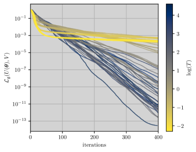
Figure 12: Compiling short-time dynamics for global Hamiltonians. For a system of $n=20$ qubits, we train an overparametrized (27-layer) ansatz to minimize $\mathcal{L}_{\mathfrak{g}}$, with a target unitary generated by a normalized global Hamiltonian. At larger values of $T$, the expected exponential convergence is observed. At $T\approx 1$, a transition is observed to a regime with poorer trainability.

F.2 Center of $\mathcal{G}_{\operatorname{TFXY}}$

In Section III.3.3, we observed that when $Z(\mathcal{G})$ is nontrivial (i.e., including non-identity terms), elements of $Z(\mathcal{G})$ can be compiled by the ansatz but cannot be distinguished by the adjoint-representation loss function $\mathcal{L}_{\mathfrak{g}}$. Here we show that there is exactly one non-trivial element of $Z(\mathcal{G}_{\operatorname{TFXY}})$ up to a global phase.

We note that for a dynamical Lie algebra $\mathfrak{g}$ and its dynamical Lie group $\mathcal{G}=e^{\mathfrak{g}}$, we have $Z(\mathcal{G})=\mathfrak{g}^{\prime}\cap\mathcal{G}$, where $\mathfrak{g}^{\prime}\equiv\{A\in\mathbb{C}^{d\times d}\mid\forall B\in\mathfrak{g},AB=BA\}$ is the commutant of $\mathfrak{g}$. Hence, given characterization of the commutant of the Lie algebra of interest, it is relatively easy to determine the center of its Lie group. For instance, we have $\mathfrak{g}^{\prime}_{\operatorname{TFXY}}=\operatorname{span}\{I,(\sigma^{z})^{\otimes n}\}$ [47], and one can see that the non-identity element of the commutant $(\sigma^{z})^{\otimes n}$ can be compiled up to a global phase, since $\sigma_{z}=ie^{-\frac{i\pi}{2}\sigma_{z}}=-ie^{-\frac{3i\pi}{4}\sigma_{z}}$. That is, $(\sigma^{z})^{\otimes n}$ can be compiled with $\sigma_{z}$ rotations on each qubit, with angles $\pi/2$ or $\pi/4$, and thus belong to $\mathcal{G}_{\operatorname{TFXY}}$. This leaves us with exactly one (non-trivial) element of the group that cannot be detected by $\mathcal{L}_{\mathfrak{g}}$.

Appendix G Implementing the binary quantum-phase classifier on a quantum device

In Section III.4, we described the training of a quantum-phase classifier, implemented via a variational ansatz circuit $U(\bm{\theta})$ defined in Eq. (37). After training, a set of optimal parameters $\bm{\theta}^{*}$ is acquired, allowing classification of unseen states using the unitary $U_{*}\equiv U(\bm{\theta}^{*})$. Straightforward implementation of the classifier on quantum hardware consists in applying the unitary $U_{*}$ to an unknown state, measuring the operator $O=\sigma^{z}_{1}$, and assigning a label according to Eq. (41). However we could also replicate the model by means of measurements and post-processing only. Indeed, while Result 1 was framed as an evolution of expectation values, it can equivalently be seen as an (Heisenberg) evolution of the observable.

Given the adjoint representation $\bar{\bm{U}}_{*}=\Phi_{\mathcal{G}}^{\operatorname{Ad}}(U_{*})$ of the trained circuit (computed in $\mathfrak{g}{\text{-}}{\rm sim}$), and a description of the observable $O\in i\mathfrak{g}$ as the vector $\bm{w}$ such that $O=\sum(\bm{w})_{\alpha}G_{\alpha}$, we have

$$O^{\prime}:=U_{*}^{\dagger}OU_{*}=\sum_{\alpha=1}^{\operatorname{dim}(\mathfrak{g})}(\bm{w}^{\prime})_{\alpha}G_{\alpha},\text{ with }\bm{w}^{\prime}=\bm{w}^{\rm T}\bar{\bm{U}}_{*}.$$ (85)

Hence, one recovers the classifier outputs as a weighted sum of the expectation values of the observables $G_{\alpha}$.

Depending on the characteristics of the quantum device at hand (i.e., measurement versus gate fidelity and cycle times), one approach may be preferred to another. For the measurement-based one, one may further reduce the amount of measurements required by pruning the model (i.e., approximating Eq. (85) with a subset of the terms involved). For instance, this could be achieved by discarding terms corresponding to small weights $|(\bm{w}^{\prime})_{\alpha}|<\delta$ for some threshold $\delta$, or by discarding greater-than-$k$-local terms. In particular, the later could be combined with classical shadows [103] by means of random measurements (rather than direct measurements of expectation values of all the $G_{\alpha}$) ensuring small approximation error due to the bounded locality.

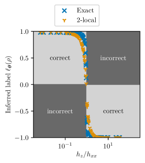
Figure 13: Comparison of exact label inferences to their 2-local approximation. We compare the exact inferred labels of the TFIM phase classifier on an unseen training dataset to a 2-local approximation. The 2-local approximation still achieves 100% classification accuracy, although $\ell_{\bm{\theta}}(\rho)$ changes less rapidly near the phase transition.

To study further the effect of such locality-pruning, we compare the accuracy of a trained classifier to its 2-local approximation, for an undisguised ($T=0$) TFIM of $n=50$ qubits. As can be seen in Figure 13, despite slight differences in the output of the models, the approximated classifier retains full accuracy (with 100% of the testing data correctly classified) that can be explained by the high locality of the TFIM order parameters.

References

- Gottesman [1997] D. Gottesman, Stabilizer codes and quantum error correction (California Institute of Technology, 1997).
- Vidal [2003] G. Vidal, Efficient classical simulation of slightly entangled quantum computations, Phys. Rev. Lett. 91, 147902 (2003).
- Valiant [2001] L. G. Valiant, Quantum computers that can be simulated classically in polynomial time, in Proceedings of the thirty-third annual ACM symposium on Theory of computing (2001) pp. 114–123.
- Terhal and DiVincenzo [2002] B. M. Terhal and D. P. DiVincenzo, Classical simulation of noninteracting-fermion quantum circuits, Physical Review A 65, 032325 (2002).
- Kim et al. [2023] Y. Kim, A. Eddins, S. Anand, K. X. Wei, E. Van Den Berg, S. Rosenblatt, H. Nayfeh, Y. Wu, M. Zaletel, K. Temme, et al., Evidence for the utility of quantum computing before fault tolerance, Nature 618, 500 (2023).
- Cerezo et al. [2021a] M. Cerezo, A. Arrasmith, R. Babbush, S. C. Benjamin, S. Endo, K. Fujii, J. R. McClean, K. Mitarai, X. Yuan, L. Cincio, and P. J. Coles, Variational quantum algorithms, Nature Reviews Physics 3, 625–644 (2021a).
- Bharti et al. [2022] K. Bharti, A. Cervera-Lierta, T. H. Kyaw, T. Haug, S. Alperin-Lea, A. Anand, M. Degroote, H. Heimonen, J. S. Kottmann, T. Menke, et al., Noisy intermediate-scale quantum algorithms, Reviews of Modern Physics 94, 015004 (2022).
- Schuld et al. [2015] M. Schuld, I. Sinayskiy, and F. Petruccione, An introduction to quantum machine learning, Contemporary Physics 56, 172 (2015).
- Biamonte et al. [2017] J. Biamonte, P. Wittek, N. Pancotti, P. Rebentrost, N. Wiebe, and S. Lloyd, Quantum machine learning, Nature 549, 195 (2017).
- Larocca et al. [2022a] M. Larocca, F. Sauvage, F. M. Sbahi, G. Verdon, P. J. Coles, and M. Cerezo, Group-invariant quantum machine learning, PRX Quantum 3, 030341 (2022a).
- Cerezo et al. [2022] M. Cerezo, G. Verdon, H.-Y. Huang, L. Cincio, and P. J. Coles, Challenges and opportunities in quantum machine learning, Nature Computational Science 10.1038/s43588-022-00311-3 (2022).
- McClean et al. [2018] J. R. McClean, S. Boixo, V. N. Smelyanskiy, R. Babbush, and H. Neven, Barren plateaus in quantum neural network training landscapes, Nature Communications 9, 1 (2018).
- Cerezo et al. [2021b] M. Cerezo, A. Sone, T. Volkoff, L. Cincio, and P. J. Coles, Cost function dependent barren plateaus in shallow parametrized quantum circuits, Nature Communications 12, 1 (2021b).
- Anschuetz and Kiani [2022] E. R. Anschuetz and B. T. Kiani, Beyond barren plateaus: Quantum variational algorithms are swamped with traps, Nature Communications 13, 7760 (2022).
- Czarnik et al. [2021] P. Czarnik, A. Arrasmith, P. J. Coles, and L. Cincio, Error mitigation with Clifford quantum-circuit data, Quantum 5, 592 (2021).
- Strikis et al. [2021] A. Strikis, D. Qin, Y. Chen, S. C. Benjamin, and Y. Li, Learning-based quantum error mitigation, PRX Quantum 2, 040330 (2021).
- Arute et al. [2020a] F. Arute, K. Arya, R. Babbush, D. Bacon, J. C. Bardin, R. Barends, A. Bengtsson, S. Boixo, M. Broughton, B. B. Buckley, et al., Observation of separated dynamics of charge and spin in the Fermi-Hubbard model, arXiv preprint arXiv:2010.07965 (2020a).
- Montanaro and Stanisic [2021] A. Montanaro and S. Stanisic, Error mitigation by training with fermionic linear optics, arXiv preprint arXiv:2102.02120 (2021).
- Matos et al. [2022] G. Matos, C. N. Self, Z. Papić, K. Meichanetzidis, and H. Dreyer, Characterization of variational quantum algorithms using free fermions, arXiv preprint arXiv:2206.06400 (2022).
- Grant et al. [2019] E. Grant, L. Wossnig, M. Ostaszewski, and M. Benedetti, An initialization strategy for addressing barren plateaus in parametrized quantum circuits, Quantum 3, 214 (2019).
- Verdon et al. [2019] G. Verdon, M. Broughton, J. R. McClean, K. J. Sung, R. Babbush, Z. Jiang, H. Neven, and M. Mohseni, Learning to learn with quantum neural networks via classical neural networks, arXiv preprint arXiv:1907.05415 (2019).
- Sauvage et al. [2021] F. Sauvage, S. Sim, A. A. Kunitsa, W. A. Simon, M. Mauri, and A. Perdomo-Ortiz, Flip: A flexible initializer for arbitrarily-sized parametrized quantum circuits, arXiv preprint arXiv:2103.08572 (2021).
- Rad et al. [2022] A. Rad, A. Seif, and N. M. Linke, Surviving the barren plateau in variational quantum circuits with bayesian learning initialization, arXiv preprint arXiv:2203.02464 (2022).
- Liu et al. [2022] X. Liu, G. Liu, J. Huang, and X. Wang, Mitigating barren plateaus of variational quantum eigensolvers, arXiv preprint arXiv:2205.13539 (2022).
- Mitarai et al. [2022] K. Mitarai, Y. Suzuki, W. Mizukami, Y. O. Nakagawa, and K. Fujii, Quadratic clifford expansion for efficient benchmarking and initialization of variational quantum algorithms, Physical Review Research 4, 033012 (2022).
- Ravi et al. [2022] G. Ravi, P. Gokhale, Y. Ding, W. Kirby, K. Smith, J. Baker, P. Love, H. Hoffmann, K. Brown, and F. Chong, Cafqa: A classical simulation bootstrap for variational quantum algorithms, arXiv preprint arXiv:2202.12924 (2022).
- Cheng et al. [2022] M. Cheng, K. Khosla, C. Self, M. Lin, B. Li, A. Medina, and M. Kim, Clifford circuit initialisation for variational quantum algorithms, arXiv preprint arXiv:2207.01539 (2022).
- Dborin et al. [2022] J. Dborin, F. Barratt, V. Wimalaweera, L. Wright, and A. G. Green, Matrix product state pre-training for quantum machine learning, Quantum Science and Technology 7, 035014 (2022).
- Mele et al. [2022] A. A. Mele, G. B. Mbeng, G. E. Santoro, M. Collura, and P. Torta, Avoiding barren plateaus via transferability of smooth solutions in Hamiltonian variational ansatz, arXiv preprint arXiv:2206.01982 (2022).
- Rudolph et al. [2022] M. S. Rudolph, J. Miller, J. Chen, A. Acharya, and A. Perdomo-Ortiz, Synergy between quantum circuits and tensor networks: Short-cutting the race to practical quantum advantage, arXiv preprint arXiv:2208.13673 (2022).
- Somma [2005] R. D. Somma, Quantum computation, complexity, and many-body physics, arXiv preprint quant-ph/0512209 (2005).
- Somma et al. [2006] R. Somma, H. Barnum, G. Ortiz, and E. Knill, Efficient solvability of Hamiltonians and limits on the power of some quantum computational models, Physical Review Letters 97, 190501 (2006).
- Anschuetz et al. [2022] E. R. Anschuetz, A. Bauer, B. T. Kiani, and S. Lloyd, Efficient classical algorithms for simulating symmetric quantum systems, arXiv preprint arXiv:2211.16998 (2022).
- Bonet-Monroig et al. [2020] X. Bonet-Monroig, R. Babbush, and T. E. O’Brien, Nearly optimal measurement scheduling for partial tomography of quantum states, Physical Review X 10, 031064 (2020).
- Kökcü et al. [2022] E. Kökcü, T. Steckmann, Y. Wang, J. Freericks, E. F. Dumitrescu, and A. F. Kemper, Fixed depth hamiltonian simulation via cartan decomposition, Physical Review Letters 129, 070501 (2022).
- Schatzki et al. [2022] L. Schatzki, M. Larocca, F. Sauvage, and M. Cerezo, Theoretical guarantees for permutation-equivariant quantum neural networks, arXiv preprint arXiv:2210.09974 (2022).
- Peruzzo et al. [2014] A. Peruzzo, J. McClean, P. Shadbolt, M.-H. Yung, X.-Q. Zhou, P. J. Love, A. Aspuru-Guzik, and J. L. O’brien, A variational eigenvalue solver on a photonic quantum processor, Nature Communications 5, 1 (2014).
- Hall [2013] B. C. Hall, Lie groups, Lie algebras, and representations (Springer, 2013).
- Kirillov Jr [2008] A. Kirillov Jr, An introduction to Lie groups and Lie algebras, 113 (Cambridge University Press, 2008).
- D’Alessandro [2007] D. D’Alessandro, Introduction to Quantum Control and Dynamics, Chapman & Hall/CRC Applied Mathematics & Nonlinear Science (Taylor & Francis, 2007).
- Zeier and Schulte-Herbrüggen [2011] R. Zeier and T. Schulte-Herbrüggen, Symmetry principles in quantum systems theory, Journal of mathematical physics 52, 113510 (2011).
- Larocca et al. [2022b] M. Larocca, P. Czarnik, K. Sharma, G. Muraleedharan, P. J. Coles, and M. Cerezo, Diagnosing Barren Plateaus with Tools from Quantum Optimal Control, Quantum 6, 824 (2022b).
- Larocca et al. [2023] M. Larocca, N. Ju, D. García-Martín, P. J. Coles, and M. Cerezo, Theory of overparametrization in quantum neural networks, Nature Computational Science 3, 542 (2023).
- Jones and Gacon [2020] T. Jones and J. Gacon, Efficient calculation of gradients in classical simulations of variational quantum algorithms, arXiv preprint arXiv:2009.02823 (2020).
- Lloyd [1995] S. Lloyd, Almost any quantum logic gate is universal, Physical Review Letters 75, 346 (1995).
- Kazi et al. [2023] S. Kazi, M. Larocca, and M. Cerezo, On the universality of -equivariant -body gates, arXiv preprint arXiv:2303.00728 (2023).
- [47] S. Kazi, M. Larocca, M. Farinati, P. Coles, R. Zeier, and M. Cerezo, The landscape of qaoa maxcut lie algebras, In preparation .
- Goh [2023] M. L. Goh, g-sim, https://github.com/gohmat/g-sim (2023).
- Bittel and Kliesch [2021] L. Bittel and M. Kliesch, Training variational quantum algorithms is NP-hard, Phys. Rev. Lett. 127, 120502 (2021).
- Neyshabur et al. [2018] B. Neyshabur, Z. Li, S. Bhojanapalli, Y. LeCun, and N. Srebro, The role of over-parametrization in generalization of neural networks, in International Conference on Learning Representations (2018).
- Zhang et al. [2021] C. Zhang, S. Bengio, M. Hardt, B. Recht, and O. Vinyals, Understanding deep learning (still) requires rethinking generalization, Communications of the ACM 64, 107 (2021).
- Allen-Zhu et al. [2019] Z. Allen-Zhu, Y. Li, and Y. Liang, Learning and generalization in overparameterized neural networks, going beyond two layers, Advances in neural information processing systems (2019).
- Du et al. [2019a] S. Du, J. Lee, H. Li, L. Wang, and X. Zhai, Gradient descent finds global minima of deep neural networks, in International Conference on Machine Learning (PMLR, 2019) pp. 1675–1685.
- Buhai et al. [2020] R.-D. Buhai, Y. Halpern, Y. Kim, A. Risteski, and D. Sontag, Empirical study of the benefits of overparameterization in learning latent variable models, in International Conference on Machine Learning (PMLR, 2020) pp. 1211–1219.
- Du et al. [2019b] S. S. Du, X. Zhai, B. Poczos, and A. Singh, Gradient descent provably optimizes over-parameterized neural networks, in International Conference on Learning Representations (2019).
- Brutzkus et al. [2018] A. Brutzkus, A. Globerson, E. Malach, and S. Shalev-Shwartz, SGD learns over-parameterized networks that provably generalize on linearly separable data, in International Conference on Learning Representations (2018).
- Wecker et al. [2015] D. Wecker, M. B. Hastings, and M. Troyer, Progress towards practical quantum variational algorithms, Physical Review A 92, 042303 (2015).
- Wiersema et al. [2020] R. Wiersema, C. Zhou, Y. de Sereville, J. F. Carrasquilla, Y. B. Kim, and H. Yuen, Exploring entanglement and optimization within the Hamiltonian variational ansatz, PRX Quantum 1, 020319 (2020).
- Ho and Hsieh [2019] W. W. Ho and T. H. Hsieh, Efficient variational simulation of non-trivial quantum states, SciPost Phys. 6, 29 (2019).
- Cade et al. [2020] C. Cade, L. Mineh, A. Montanaro, and S. Stanisic, Strategies for solving the Fermi-Hubbard model on near-term quantum computers, Physical Review B 102, 235122 (2020).
- Cerezo et al. [2021c] M. Cerezo, A. Sone, T. Volkoff, L. Cincio, and P. J. Coles, Cost function dependent barren plateaus in shallow parametrized quantum circuits, Nature Communications 12, 1 (2021c).
- Holmes et al. [2022] Z. Holmes, K. Sharma, M. Cerezo, and P. J. Coles, Connecting ansatz expressibility to gradient magnitudes and barren plateaus, PRX Quantum 3, 010313 (2022).
- Arrasmith et al. [2022] A. Arrasmith, Z. Holmes, M. Cerezo, and P. J. Coles, Equivalence of quantum barren plateaus to cost concentration and narrow gorges, Quantum Science and Technology 7, 045015 (2022).
- Broughton et al. [2020] M. Broughton, G. Verdon, T. McCourt, A. J. Martinez, J. H. Yoo, S. V. Isakov, P. Massey, R. Halavati, M. Yuezhen Niu, A. Zlokapa, E. Peters, O. Lockwood, A. Skolik, S. Jerbi, V. Dunjko, M. Leib, M. Streif, D. Von Dollen, H. Chen, S. Cao, R. Wiersema, H.-Y. Huang, J. R. McClean, R. Babbush, S. Boixo, D. Bacon, A. K. Ho, H. Neven, and M. Mohseni, Tensorflow quantum: A software framework for quantum machine learning, arXiv preprint arXiv:2003.02989 (2020).
- Farhi et al. [2014] E. Farhi, J. Goldstone, and S. Gutmann, A quantum approximate optimization algorithm, arXiv preprint arXiv:1411.4028 (2014).
- Goemans and Williamson [1995] M. X. Goemans and D. P. Williamson, Improved approximation algorithms for maximum cut and satisfiability problems using semidefinite programming, Journal of the ACM (JACM) 42, 1115 (1995).
- Ozaeta et al. [2022] A. Ozaeta, W. van Dam, and P. L. McMahon, Expectation values from the single-layer quantum approximate optimization algorithm on ising problems, Quantum Science and Technology 7, 045036 (2022).
- Zhou et al. [2020] L. Zhou, S.-T. Wang, S. Choi, H. Pichler, and M. D. Lukin, Quantum approximate optimization algorithm: Performance, mechanism, and implementation on near-term devices, Physical Review X 10, 021067 (2020).
- Koßmann et al. [2022] G. Koßmann, L. Binkowski, L. van Luijk, T. Ziegler, and R. Schwonnek, Deep-circuit qaoa, arXiv preprint arXiv:2210.12406 (2022).
- Oszmaniec et al. [2022] M. Oszmaniec, N. Dangniam, M. E. Morales, and Z. Zimborás, Fermion sampling: a robust quantum computational advantage scheme using fermionic linear optics and magic input states, PRX Quantum 3, 020328 (2022).
- Khatri et al. [2019] S. Khatri, R. LaRose, A. Poremba, L. Cincio, A. T. Sornborger, and P. J. Coles, Quantum-assisted quantum compiling, Quantum 3, 140 (2019).
- Sharma et al. [2020] K. Sharma, S. Khatri, M. Cerezo, and P. J. Coles, Noise resilience of variational quantum compiling, New Journal of Physics 22, 043006 (2020).
- Caro et al. [2022] M. C. Caro, H.-Y. Huang, N. Ezzell, J. Gibbs, A. T. Sornborger, L. Cincio, P. J. Coles, and Z. Holmes, Out-of-distribution generalization for learning quantum dynamics, arXiv preprint arXiv:2204.10268 (2022).
- Gibbs et al. [2022] J. Gibbs, Z. Holmes, M. C. Caro, N. Ezzell, H.-Y. Huang, L. Cincio, A. T. Sornborger, and P. J. Coles, Dynamical simulation via quantum machine learning with provable generalization, arXiv preprint arXiv:2204.10269 (2022).
- Kökcü et al. [2021] E. Kökcü, T. Steckmann, J. Freericks, E. F. Dumitrescu, and A. F. Kemper, Fixed depth Hamiltonian simulation via Cartan decomposition, arXiv preprint arXiv:2104.00728 (2021).
- Anderson [1958] P. W. Anderson, Absence of diffusion in certain random lattices, Physical review 109, 1492 (1958).
- Cirstoiu et al. [2020] C. Cirstoiu, Z. Holmes, J. Iosue, L. Cincio, P. J. Coles, and A. Sornborger, Variational fast forwarding for quantum simulation beyond the coherence time, npj Quantum Information 6, 1 (2020).
- Bucaj [2016] V. Bucaj, On the kunz-souillard approach to localization for the discrete one dimensional generalized anderson model, arXiv preprint arXiv:1608.01379 (2016).
- Kivlichan et al. [2018] I. D. Kivlichan, J. McClean, N. Wiebe, C. Gidney, A. Aspuru-Guzik, G. K.-L. Chan, and R. Babbush, Quantum simulation of electronic structure with linear depth and connectivity, Physical review letters 120, 110501 (2018).
- Arute et al. [2020b] F. Arute, K. Arya, R. Babbush, D. Bacon, J. C. Bardin, R. Barends, S. Boixo, M. Broughton, B. B. Buckley, D. A. Buell, et al., Hartree-fock on a superconducting qubit quantum computer, Science 369, 1084 (2020b).
- Zanardi and Rasetti [1997] P. Zanardi and M. Rasetti, Noiseless quantum codes, Physical Review Letters 79, 3306 (1997).
- Eastin and Knill [2009] B. Eastin and E. Knill, Restrictions on transversal encoded quantum gate sets, Physical review letters 102, 110502 (2009).
- Khaneja et al. [2001] N. Khaneja, R. Brockett, and S. J. Glaser, Time optimal control in spin systems, Physical Review A 63, 032308 (2001).
- Zimborás et al. [2015] Z. Zimborás, R. Zeier, T. Schulte-Herbrüggen, and D. Burgarth, Symmetry criteria for quantum simulability of effective interactions, Physical Review A 92, 042309 (2015).
- Marvian [2022] I. Marvian, Restrictions on realizable unitary operations imposed by symmetry and locality, Nature Physics 18, 283 (2022).
- Yen and Izmaylov [2021] T.-C. Yen and A. F. Izmaylov, Cartan subalgebra approach to efficient measurements of quantum observables, PRX Quantum 2, 040320 (2021).
- Steckmann et al. [2021] T. Steckmann, T. Keen, A. F. Kemper, E. F. Dumitrescu, and Y. Wang, Simulating the mott transition on a noisy digital quantum computer via cartan-based fast-forwarding circuits, arXiv preprint arXiv:2112.05688 (2021).
- Cai et al. [2022] Z. Cai, R. Babbush, S. C. Benjamin, S. Endo, W. J. Huggins, Y. Li, J. R. McClean, and T. E. O’Brien, Quantum error mitigation, arXiv preprint arXiv:2210.00921 (2022).
- Knill et al. [2008] E. Knill, D. Leibfried, R. Reichle, J. Britton, R. B. Blakestad, J. D. Jost, C. Langer, R. Ozeri, S. Seidelin, and D. J. Wineland, Randomized benchmarking of quantum gates, Physical Review A 77, 012307 (2008).
- Helsen et al. [2022] J. Helsen, S. Nezami, M. Reagor, and M. Walter, Matchgate benchmarking: Scalable benchmarking of a continuous family of many-qubit gates, Quantum 6, 657 (2022).
- Lamata et al. [2018] L. Lamata, A. Parra-Rodriguez, M. Sanz, and E. Solano, Digital-analog quantum simulations with superconducting circuits, Advances in Physics: X 3, 1457981 (2018).
- Parra-Rodriguez et al. [2020] A. Parra-Rodriguez, P. Lougovski, L. Lamata, E. Solano, and M. Sanz, Digital-analog quantum computation, Physical Review A 101, 022305 (2020).
- Meitei et al. [2020] O. R. Meitei, B. T. Gard, G. S. Barron, D. P. Pappas, S. E. Economou, E. Barnes, and N. J. Mayhall, Gate-free state preparation for fast variational quantum eigensolver simulations: ctrl-vqe, arXiv preprint arXiv:2008.04302 (2020).
- Henriet et al. [2020] L. Henriet, L. Beguin, A. Signoles, T. Lahaye, A. Browaeys, G.-O. Reymond, and C. Jurczak, Quantum computing with neutral atoms, Quantum 4, 327 (2020).
- Daley et al. [2022] A. J. Daley, I. Bloch, C. Kokail, S. Flannigan, N. Pearson, M. Troyer, and P. Zoller, Practical quantum advantage in quantum simulation, Nature 607, 667 (2022).
- Wurtz et al. [2023] J. Wurtz, A. Bylinskii, B. Braverman, J. Amato-Grill, S. H. Cantu, F. Huber, A. Lukin, F. Liu, P. Weinberg, J. Long, et al., Aquila: Quera’s 256-qubit neutral-atom quantum computer, arXiv preprint arXiv:2306.11727 (2023).
- Richards [2015] A. Richards, University of oxford advanced research computing, DOI: 10.5281/zenodo.22558 (2015).
- Côté et al. [2022] J. Côté, F. Sauvage, M. Larocca, M. Jonsson, L. Cincio, and T. Albash, Diabatic quantum annealing for the frustrated ring model, arXiv preprint arXiv:2212.02624 (2022).
- Machnes et al. [2018] S. Machnes, E. Assémat, D. Tannor, and F. K. Wilhelm, Tunable, flexible, and efficient optimization of control pulses for practical qubits, Physical review letters 120, 150401 (2018).
- Chen et al. [2018] R. T. Chen, Y. Rubanova, J. Bettencourt, and D. K. Duvenaud, Neural ordinary differential equations, Advances in neural information processing systems 31 (2018).
- Schäfer et al. [2020] F. Schäfer, M. Kloc, C. Bruder, and N. Lörch, A differentiable programming method for quantum control, Machine Learning: Science and Technology 1, 035009 (2020).
- Sauvage and Mintert [2022] F. Sauvage and F. Mintert, Optimal control of families of quantum gates, Physical Review Letters 129, 050507 (2022).
- Huang et al. [2020] H.-Y. Huang, R. Kueng, and J. Preskill, Predicting many properties of a quantum system from very few measurements, Nature Physics 16, 1050 (2020).