Abstract

Perturbative calculations predict that the effective potential of the Standard Model should have a new minimum, well beyond the Planck scale, which is much deeper than the electroweak vacuum. Since it is not obvious that gravitational effects can become so strong to stabilise the potential, most authors have accepted the metastability scenario in a cosmological perspective. This perspective is needed to explain why the theory remains trapped into our electroweak vacuum, but requires to control the properties of matter in the extreme conditions of the early universe. As an alternative, one can consider the completely different idea of a non-perturbative effective potential which, as at the beginning of the Standard Model, is restricted to the pure $\Phi^{4}$ sector but is consistent with the now existing analytical and numerical studies. In this approach, where the electroweak vacuum is the lowest-energy state, beside the resonance of mass $m_{h}=$ 125 GeV defined by the quadratic shape of the potential at its minimum, the Higgs field should exhibit a second resonance with mass $(M_{H})^{\rm Theor}=690\pm 10\,({\rm stat})\pm 20\,({\rm sys})$ GeV associated with the zero-point energy which determines the potential depth. In spite of its large mass, this would couple to longitudinal W’s with the same typical strength as the low-mass state at 125 GeV and represent a relatively narrow resonance mainly produced at LHC by gluon-gluon fusion. Therefore, it is interesting that, in the LHC data, one can find combined indications for a new resonance of mass $(M_{H})^{\rm comb}\sim 682(10)$ GeV with a statistical significance that is far from negligible. Since this non-negligible evidence could become an important new discovery by just adding two missing samples of RUN2 data, we outline further refinements of the theoretical predictions that could be obtained by implementing the unitarity constraints, in the presence of fermion and gauge fields, with the type of coupled-channel calculations used in meson spectroscopy.

1 Introduction

The discovery at CERN [1, 2] of the narrow scalar resonance with mass $m_{h}\!=\!$ 125 GeV and the consistency of its phenomenology with the theoretical expectations for the Higgs boson have confirmed spontaneous symmetry breaking (SSB) through the Higgs field as a fundamental ingredient of current particle physics. Nevertheless, in our opinion there may be room for improving on the present description of symmetry breaking. The latter is based on a classical double-well potential with perturbative quantum corrections, say $V^{\rm(p)}(\phi)$, exhibiting a local minimum at $\phi\!=\!v\sim 246$ GeV and with a quadratic shape fixed by $m^{2}_{h}\!=\!(125\;\mbox{GeV})^{2}$. The point is that, at large values of $\phi$, this potential is well approximated as $V^{\rm(p)}(\phi)\sim\lambda^{\rm(p)}(\phi)\,\phi^{4}$, in terms of the perturbative scalar coupling $\lambda^{\rm(p)}(\phi)$ which includes the effect of the gauge and fermion fields and becomes negative beyond an instability scale $\phi_{\rm inst}\sim 10^{10}$ GeV. As a net result, besides the local electroweak vacuum where $V^{\rm(p)}(v)\sim-10^{8}\;\mbox{GeV}^{4}$, the true, absolute minimum of this perturbative potential is at $v_{\rm true}\sim 10^{26}\div 10^{31}$ GeV [3, 4] (depending on the approximations and the exact values of the input parameters), with a much deeper potential value $V^{\rm(p)}(v_{\rm true})\sim-(10^{100}\div 10^{120})$ (GeV)⁴.

While it is reassuring that the most accurate calculation [5] gives a tunneling time which is larger than the age of the universe, still the idea of a metastable vacuum raises several questions. For instance, the new minimum is much larger than the Planck mass $M_{P}$ and the Planck scale is usually regarded as the scale where gravity becomes strong. Thus, should the problem at large $\phi\sim M_{P}$ be formulated in a curved space-time? In this case, does the second minimum disappear? Here, due to various uncertainties, there is no general consensus [6, 7] that gravitational physics at the Planck scale can become so strong to stabilise the electroweak vacuum. On the contrary, the vanishing value of the observed cosmological constant, on a particle-physics scale, could imply that gravity remains weak [4] at all energies without introducing any threshold effect near $M_{P}$.

Thus, one has been considering the metastability scenario in a cosmological perspective, because in an infinitely old universe even an arbitrarily small tunneling probability would be incompatible with our existence [8]. However, given the extreme conditions in the early universe, the survival of the tiny electroweak minimum is somewhat surprising. As an example, before the discovery of the resonance at 125 GeV, the authors of Ref. [9] were concluding that, for $114\;\mbox{GeV}\leq m_{h}\leq 130$ GeV and from the analysis of cosmological perturbations, either we live in a very special and exponentially unlikely corner or new physics must exist below $\phi_{\rm inst}\sim 10^{10}$ GeV.

As an alternative, one can consider the completely different idea of a non-perturbative effective potential. Indeed, if SSB represents a non-perturbative phenomenon, one may try to also describe it non-perturbatively. Since this cannot be done by retaining the full gauge and fermion structure of the theory, as in the early days of the Standard Model, one could first concentrate on the pure $\Phi^{4}$ sector. Nonetheless, in view of the substantial theoretical progress over the past fifty years, this implies trying to describe SSB consistently with the existing theoretical and numerical studies. Obtaining such a description is a preliminary step in comparing the contributions of the various sectors to vacuum stability and then, eventually, to conclude that SSB is basically a phenomenon arising within pure $\Phi^{4}$ theory.

This problem has already been addressed in Refs. [10, 11, 12], by first following the indications of lattice simulations [13, 14, 15] that support a view of SSB in $\Phi^{4}$ as a weak first-order phase transition, and then considering the known approximations to the effective potential that are consistent with both this scenario and the basic “triviality” property of the theory. Since these approximations, albeit physically equivalent, resum to all orders different classes of diagrams, the resulting scheme can be considered non-perturbative. In this way, one obtains a picture where the (absolute) electroweak minimum of the potential can coexist with a quadratic shape $V^{\prime\prime}_{\rm eff}(\phi\!=\!0)=m^{2}_{\Phi}>0$ that is very small yet still positive. This leads to an intuitive picture of the broken-symmetry phase as a condensate of physical quanta with mass $m_{\Phi}$ whose collective self-interaction represents the primary sector that induces SSB.

The main new feature of this first-order description of SSB is that the mass scale $M_{H}$ associated with the zero-point energy (ZPE), and which determines the potential depth, is much larger than the mass scale $m_{h}$ defined by the quadratic shape of the potential at its minimum. This is because, differently from the second-order scenario where the instability of the symmetric phase is driven by a negative mass squared, ZPEs have now to compensate for a tree-level potential that otherwise would have no non-trivial minimum. The large difference of the two mass scales produces an ambiguity in the definition of the vacuum field $v\sim 246$ GeV that has no counterpart in the usual perturbative approach. Resolving this ambiguity requires a Renormalisation-Group (RG) analysis of the SSB phenomenon, which is essential to conclude that the contribution of the gauge and fermion fields to vacuum stability can be considered a small radiative correction.

Such an RG analysis is needed because the quartic coupling $\lambda\!=\!\lambda(\mu)$ associated with the self-interaction of the primary scalar sector is positive definite and exhibits a Landau pole $\Lambda$. This is linked to the distance $r_{0}\!\sim\!\Lambda^{-1}$ at which the elementary quanta feel a hard-core repulsion, while at a finite scale $\mu$ one has $\lambda(\mu)\!\sim\!L^{-1}$ in terms of $L\!=\!\ln(\Lambda/\mu)$. Now, since for any non-zero $\lambda$ there is a Landau pole $\Lambda$, one can improve the description by considering the set of theories ($\Lambda$,$\lambda$), ($\Lambda^{\prime}$,$\lambda^{\prime}$), ($\Lambda^{\prime\prime}$,$\lambda^{\prime\prime}$), …with larger and larger Landau poles, smaller and smaller low-energy couplings at $\mu$, but all having the same depth of the potential at the minimum $\phi\!=\!\phi_{v}$, i.e., with the same vacuum energy $\mathcal{E}\!=\!V_{\rm eff}(\phi_{v})$ as determined by the equation

$$\left(\Lambda\frac{\partial}{\partial\Lambda}+\Lambda\frac{\partial\lambda}{\partial\Lambda}\frac{\partial}{\partial\lambda}\right){\cal E}(\lambda,\Lambda)\;=\;0\;.$$ (1)

This requirement derives from imposing RG invariance of the effective potential in the three-dimensional space ($\phi$, $\lambda$, $\Lambda$) [10, 11, 12], namely

$$\left(\Lambda\frac{\partial}{\partial\Lambda}+\Lambda\frac{\partial\lambda}{\partial\Lambda}\frac{\partial}{\partial\lambda}+\Lambda\frac{\partial\phi}{\partial\Lambda}\frac{\partial}{\partial\phi}\right)V_{\rm eff}(\phi,\lambda,\Lambda)\;=\;0\;,$$ (2)

and can in principle also allow one to handle the $\Lambda\!\to\!\infty$ limit. Now, in those known approximations to the effective potential that are consistent with “triviality” and a weak first-order scenario of SSB, in terms of the ZPE mass scale $M_{H}$ one finds ${\cal E}=V_{\rm eff}(\phi_{v})\sim-M^{4}_{H}$. By Eq. (1) this means that $M_{H}\sim\Lambda\exp(-1/\lambda)$ is an RG-invariant mass scale $I_{1}=M_{H}$ or, equivalently, that $M_{H}$ is the scale within the logarithm $L=\ln(\Lambda/M_{H})$ in the low-energy coupling $\lambda\sim L^{-1}$. However, for the same reason the relation $M^{2}_{H}\sim\lambda\phi^{2}_{v}\sim\phi^{2}_{v}L^{-1}$ implies that $\phi_{v}\sim M_{H}L^{1/2}$ cannot represent the Fermi scale, which is always assumed to be a cutoff-independent quantity. Analogously, the quadratic shape of the potential, which is obtained by twice differentiating the potential with respect to the cutoff-dependent $\phi_{v}$, will be much smaller than $M_{H}$, namely $m^{2}_{h}=V^{\prime\prime}_{\rm eff}(\phi_{v})\sim M^{2}_{H}L^{-1}$.

A solution to this problem can be found by noticing that in the RG analysis there is a second invariant $I_{2}$ [10, 11, 12], related to a particular normalisation of the vacuum field and in terms of which the minimisation of the energy can be expressed as $I_{1}=KI_{2}$, with $K$ being a cutoff-independent constant. This $I_{2}$ is then the candidate to represent the weak scale, i.e., $I_{2}\!=\!v\sim 246$ GeV, giving $M_{H}=Kv$. Since a cutoff-independent $v$ should scale as $v\sim\phi_{v}\sqrt{\lambda}\sim\phi_{v}L^{-1/2}$ and $m_{h}\sim M_{H}L^{-1/2}$, the natural relation between $v$ and $\phi_{v}$ thus becomes

$$v\;=\;\frac{m_{h}}{M_{H}}\,\phi_{v}\;.$$ (3)

This way, with

$$\frac{3M^{2}_{H}}{\phi^{2}_{v}}\;=\;\frac{3m^{2}_{h}}{v^{2}}\;,$$ (4)

the two fourth-order scalar couplings have the same value at the Fermi scale $\mu\!\sim\!v$, namely

$$\lambda(v)\;=\;\lambda^{\rm(p)}(v)\;=\;3m^{2}_{h}/v^{2}\;,$$ (5)

while still behaving quite differently at very large $\mu$.

Now, if the higher-momentum mass scale $M_{H}$, associated with ZPEs, differs non-trivially from the zero-momentum mass scale $m_{h}$ defined by the quadratic shape of the potential at its minimum, the Higgs field propagator should deviate from a standard one-pole structure. The existence of these deviations has been checked with lattice simulations of the propagator, which have also confirmed the expected scaling trend $M^{2}_{H}\sim m^{2}_{h}L$ [10]. Thus one arrives at the conclusion that, besides the known resonance with $m_{h}\!=\!125$ GeV, there should be a second resonance with a much larger mass, which by combining numerical and analytical relations can be estimated to have a value $M_{H}\!\sim\!700$ GeV. With such a large $M_{H}$, the ZPEs of all known gauge and fermion fields would represent a small radiative correction, so that, by restricting to experiments in a region around the Fermi scale, say a few TeV, the different evolution of $\lambda^{\rm(p)}(\mu)$ and $\lambda(\mu)$ at asymptotically large $\mu$ should remain unobservable. The crucial check of our picture is then the necessity to experimentally observe the second resonance. Its discovery would mean that SSB is a phenomenon originating within the primary scalar sector, namely from the collective self-interaction of the basic quanta of the symmetric phase.

After outlining in Sec. 2 the weak first-order picture of SSB, we will consider in Sec. 3 the basic phenomenology of the second resonance. In Sec. 4 we will then summarise some recent analyses [16, 17, 18, 19] of LHC data that indeed support the existence of a new resonance in the expected mass range. As we will show, the present non-negligible statistical evidence could become an important new discovery by adding two crucial, still missing samples of RUN2 data. In view of these possible future developments, we will illustrate in Sec. 5 the basic ingredients of a coupled-channel calculation, which could be useful to further refine the theoretical predictions for the mass and width of the hypothetical new resonance when interacting with the gauge and fermion sectors of the Standard Model. Section 6 will be devoted to our conclusions, besides some remarks about the present agreement between the Higgs-mass parameter extracted indirectly from radiative corrections and the value $m_{h}=125$ GeV directly measured at the LHC.

2 SSB in a $\Phi^{4}$ theory

2.1 Preliminaries

Let us start from scratch with the type of scalar potential reported in the review of the Particle Data Group (PDG) [20]:

$$V_{\rm PDG}(\phi)\;=\;-\frac{1}{2}m^{2}_{\rm PDG}\,\phi^{2}+\frac{1}{4!}\lambda_{\rm PDG}\,\phi^{4}\;.$$ (6)

By fixing $m_{\rm PDG}\sim 88.8$ GeV and $\lambda_{\rm PDG}\sim 0.78$, this has a minimum at $|\phi|=v\sim 246$ GeV and a second derivative $V^{\prime\prime}_{\rm PDG}(v)\equiv m^{2}_{h}=$ (125 GeV)² (one is adopting here the identification $m^{2}_{h}=V^{\prime\prime}_{\rm PDG}(v)=|G^{-1}(p=0)|$ in terms of the inverse, zero-momentum propagator).

In Eq. (6), one is assuming a double-well potential with suitably chosen mass and coupling. The instability of the symmetric vacuum at $\phi=0$ is then traced back to the condition $V^{\prime\prime}_{\rm PDG}(\phi=0)=-m^{2}_{\rm PDG}<0$, which characterises SSB as a second-order phase transition. This traditional idea of a “tachyonic” mass term at $\phi=0$, however, is not the only possible explanation. As in the original analysis by Coleman and Weinberg [21], SSB could originate from the ZPE in the classically scale invariant limit $V^{\prime\prime}_{\rm eff}(\phi=0)\to 0^{+}$. In this case, if the quanta of the symmetric phase have a tiny physical mass $m^{2}_{\Phi}\equiv V^{\prime\prime}_{\rm eff}(\phi=0)>0$ below some critical value $m^{2}_{c}$, the symmetric phase could be “locally” stable but become “globally” unstable. By lowering the mass below $m^{2}_{c}$, the absolute minimum of the effective potential would then discontinuously jump from $\phi=0$ to $\phi\neq 0$ and SSB would represent a first-order phase transition.

In order to understand how subtle the issue can be and get some intuitive insight, let us consider the following toy model:

$$V_{\rm toy}(\phi)\;=\;\frac{1}{2}m^{2}\phi^{2}+\frac{1}{4!}\lambda\phi^{4}\left(1+\epsilon\ln\frac{\phi^{2}}{\mu^{2}}\right)\;,$$ (7)

where $\mu$ is some mass scale and $\epsilon$ is a small, positive parameter (the quantum-theory case is with $\epsilon\sim\lambda$, but in this toy model we treat $\epsilon$ as a separate parameter). For $\epsilon=0$, where $V_{\rm toy}(\phi)$ reduces to the classical potential $V_{\rm cl}(\phi)$, by varying the $m^{2}$ parameter there is a second-order phase transition at $m^{2}=0$ . However, for any $\epsilon>0$, no matter how small, one has a first-order transition, occurring at a positive $m^{2}$. The size of the critical $m^{2}_{c}$ is exponentially small, viz. $\mu^{2}\exp(-1/\epsilon)$, meaning that an infinitesimally weak first-order transition can become indistinguishable from a second-order transition, unless one looks on a fine enough scale.

We emphasise that this idea of SSB as a weak first-order phase transition in $\Phi^{4}$ theories finds support in lattice simulations [13, 14, 15]. To that end, one can just look at Fig. 7 in Ref. [15], where the data for the average field at the critical temperature show the characteristic first-order jump and not the smooth second-order trend. This agreement with lattice simulations is a good motivation to further explore the physical implications of a first-order scenario.

From a purely physical point of view, the underlying rationale for a tachyonic mass term at $\phi=0$ reflects the basic prejudice that $\Phi^{4}$ is an interaction that is always repulsive. In fact, with a purely repulsive interaction, any state made of massive physical particles, would necessarily have an energy density that is higher than the trivial empty vacuum at $\phi=0$. However, as discussed in Ref. [24], the $\Phi^{4}$ interaction is not always repulsive. The interparticle potential between the basic quanta of the symmetric phase, besides the $+\lambda\,\delta^{3}(\bf r)$ tree-level repulsion, contains a $-\lambda^{2}\,e^{-2m_{\Phi}r}/r^{3}$ attraction, which originates in the ultraviolet-finite part of the one-loop diagrams and whose range becomes longer and longer in the $m_{\Phi}\to 0$ limit. Due to the qualitative difference between the two effects and in order to consistently include higher-order effects, one should rearrange the perturbative expansion by symmetrically renormalising both the contact repulsion and the long-range attraction as discussed by Stevenson [27]. In this way, by taking into account both effects, a calculation of the energy density indicates that, for positive and small enough $m_{\Phi}$, the attractive tail dominates. Then, the lowest-energy state is not the trivial, empty vacuum with $\phi=0$, but a state with $\phi\neq 0$ and a Bose condensate of symmetric-phase quanta in the $\vec{k}=\vec{0}$ mode.

2.2 “Triviality” and the effective potential

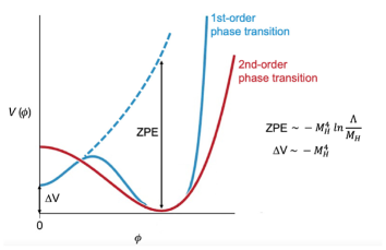
Figure 1: An intuitive picture that illustrates the crucial role of the ZPE in a first-order scenario of SSB. Differently from the standard second-order picture, it has to compensate for a tree-level potential with no non-trivial minimum.

In spite of these interesting aspects, one could still wonder about different observable consequences. After all, the phenomenology of the broken-symmetry phase should only depend on the potential near the true minimum (so not at $\phi=0$) and, in principle, nothing prevents it locally from having exactly the same shape as in Eq. (6). To get some insight, let us look at Fig. 1. This intuitively illustrates that, if $V^{\prime\prime}_{\rm eff}(\phi=0)>0$, ZPEs are expected to be much larger than in a second-order picture. In the latter case, in fact, SSB is driven by the negative mass squared at $\phi=0$, while now ZPEs have to overwhelm a tree-level potential that otherwise would have no non-trivial minimum. But what do we exactly mean by saying that ZPEs have to be much larger? The answer is that, now, the ZPE mass scale $M_{H}$ is much larger than the mass scale $m_{h}$ defined by the quadratic shape of the effective potential at the minimum. To fully understand this crucial issue let us first recall that this large size of ZPEs induced Coleman and Weinberg to expect that the weak, first-order scenario could only work in the presence of gauge bosons. In a pure $\Phi^{4}$ theory, SSB would require to compensate the positive $\lambda\phi^{4}$ tree-level potential with a negative $\lambda^{2}\phi^{4}\ln(\phi^{2}/\Lambda^{2})$ one-loop contribution, a requirement that lies outside a standard loop-expansion perspective. Instead, they concluded that with gauge bosons the corresponding one-loop contribution $g^{4}_{\rm gauge}\phi^{4}\ln(\phi^{2}/\Lambda^{2})$ could well represent the needed driving mechanism if $\lambda\sim g^{4}_{\rm gauge}$.

Nevertheless, there is a way to rearrange things in the effective potential and consistently describe SSB as first-order transition. The standard perspective, which is behind the idea of the perturbative potential $V^{\rm(p)}(\phi)\sim\lambda^{\rm(p)}(\phi)\phi^{4}$, considers the one-loop contribution as simply renormalising the coupling $\lambda$ in the classical potential

$$\frac{\lambda}{4!}\,\phi^{4}\;\to\;\frac{\lambda}{4!}\,\phi^{4}\left\{\!1-\frac{3\lambda}{32\pi^{2}}\ln\left(\frac{2\Lambda^{2}\sqrt{e}}{\lambda\phi^{2}}\right)\right\}\;.$$ (8)

Therefore, including the higher-order leading logarithmic terms, i.e., by replacing

$$1-x\to 1-x+x^{2}-x^{3}\pm\ldots\;=\;1/(1+x)\;,$$ (9)

the one-loop minimum would disappear.

But, as emphasised by Stevenson [27], the qualitatively different nature of the two basic terms in the inter-particle potential between the quanta of the symmetric phase has a definite counterpart in the structure of the effective potential. Here, the positive $\lambda\phi^{4}$ background originates from the +$\lambda\delta^{3}(\bf r)$ short-range repulsion and the negative ZPE from the long-range $-\frac{\lambda^{2}}{r^{3}}$ attraction. This observation suggests to consider the equivalent reading of the one-loop potential as the sum of a classical background plus ZPEs of free-field fluctuations with mass squared $M^{2}(\phi)=\lambda\phi^{2}/2$

$$V_{\mbox{\scriptsize 1-loop}}(\phi)=\frac{\lambda\phi^{4}}{4!}-\frac{M^{4}(\phi)}{64\pi^{2}}\ln\frac{\Lambda^{2}\sqrt{e}}{M^{2}(\phi)}.$$ (10)

Since this type of structure is also recovered in higher-order approximations, the simple one-loop potential can also admit a non-perturbative interpretation as the prototype of a class of calculations with the same basic structure up to a redefinition of both the classical background and the mass parameter $M(\phi)$.

This is explicitly illustrated by the Gaussian effective potential [30] which re-sums all one-loop bubbles and preserves the same structure up to terms that vanish when $\Lambda\to\infty$:

$$\lambda\;\to\;\lambda_{G}(\phi)\;=\;\frac{\lambda}{1+\frac{\lambda}{16\pi^{2}}\ln\frac{\Lambda}{M_{G}(\phi)}}\;,$$ (11)

$$M^{2}(\phi)\;\to\;M^{2}_{G}(\phi)\;=\;\frac{\lambda_{G}(\phi)\phi^{2}}{2}\;,$$ (12)

$$V_{\mbox{\scriptsize 1-loop}}(\phi)\!\to\!V_{G}(\phi)=\frac{\lambda_{G}(\phi)\phi^{4}}{4!}-\frac{M^{4}_{G}(\phi)}{64\pi^{2}}\ln\frac{\Lambda^{2}\sqrt{e}}{M^{2}_{G}(\phi)}.$$ (13)

The agreement between the one-loop and Gaussian effective potential has to be emphasised, because it gives further insight into the “triviality” of $\Phi^{4}$. If, in the continuum limit, all interaction effects have to be effectively reabsorbed into the first two moments of a Gaussian distribution, meaningful approximations to the effective potential should be physically equivalent to the one-loop result, i.e., given again by some classical background + ZPE of free-field fluctuations with some $\phi-$dependent mass .

For this reason, as anticipated in the Introduction, the two approximations considered above produce equivalent results. Namely, by using the same notation $\phi=\phi_{v}$ for the minimum of the effective potential, either when $V_{\rm eff}(\phi)=V_{\mbox{\scriptsize 1-loop}}(\phi)$ or when $V_{\rm eff}(\phi)=V_{G}(\phi)$, and by denoting $M_{H}$ as the value of $M(\phi_{v})$ or of $M_{G}(\phi_{v})$, one finds $V_{\rm eff}(\phi_{v})=-M^{4}_{H}/(128\pi^{2})$ and $M^{2}_{H}\sim\lambda\phi^{2}_{v}\sim\Lambda^{2}\exp(-1/\lambda)$. The important point is that the vacuum energy is an RG-invariant quantity satisfying Eq. (1), so that $M_{H}$ is $\Lambda$-independent and one can express $\lambda\sim{L}^{-1}$, with $L=\ln(\Lambda/M_{H})$.

However, for the same reason $\phi_{v}\sim M_{H}{L}^{1/2}$ cannot represent the Fermi scale, which is always assumed to be a cutoff-independent quantity. Nevertheless, since $m^{2}_{h}=V^{\prime\prime}_{\rm eff}(\phi_{v})\sim\lambda^{2}\phi^{2}_{v}\sim M^{2}_{H}{L}^{-1}$ as anticipated in the Introduction, through Eq. (3) one can introduce a vacuum field $v$ that scales uniformly with $M_{H}$ and is therefore cutoff-independent. This way, one finally obtains the following pattern of scales [10, 11, 12]:

$$\lambda\sim{L}^{-1},\;m^{2}_{h}\sim v^{2}\,{L}^{-1},\;M^{2}_{H}\sim L\,m^{2}_{h}=K^{2}v^{2},$$ (14)

where $K$ is a cutoff-independent constant and

$$\phi^{2}_{v}\;\equiv\;Z_{\phi}v^{2}\;,\;\;\;{\rm with}\;\;\;Z_{\phi}\;=\;(M_{H}/m_{h})^{2}\sim L\;.$$ (15)

Then, $M_{H}$ and $v$ will emerge as the two invariants [10, 11, 12] $I_{1}=M_{H}$ and $I_{2}=v$ associated with the analysis of the effective potential in the $(\lambda,\phi,\Lambda$) three-dimensional space, in terms of which the absolute-minimum condition can be expressed as $I_{1}=KI_{2}$. For this reason, $v$ represents the natural candidate to represent the weak scale $v\sim 246$ GeV. Note that in perturbation theory in the standard second-order scenario, where $m_{h}\sim M_{H}$, there is no $v$-$\phi_{v}$ distinction. Instead, here it is a consequence of minimising the effective potential and the strong cancelations between formally higher-order and tree-level terms. Further implications of this two-mass structure will be illustrated in the following two subsections.

2.3 The coexistence of $m_{h}$ and $M_{H}$

To further sharpen the meaning of $m_{h}$ and $M_{H}$, let us recall that the ZPE is (one half of) the trace of the logarithm of the inverse propagator $G^{-1}(p)=(p^{2}-\Pi(p))$. Therefore, in a free-field theory, where $V_{\rm free}(\phi)=m^{2}\phi^{2}/2$ and $|\Pi(p)|=|\Pi(p=0)|\equiv m^{2}$, one finds, after subtracting constant terms and quadratic divergences (or using D-dimensional regularisation with the identification $\ln\Lambda=1/(4-D)-1/2\>[\gamma-\ln(4\pi)\,]$),

$$({\rm ZPE})^{\rm free} = \frac{1}{2}\int\!\!\frac{d^{4}p}{(2\pi)^{4}}\ln(p^{2}+m^{2})\;=\;$$ (16)

$$-\frac{m^{4}}{64\pi^{2}}\!\left[\ln\frac{\Lambda^{2}}{m^{2}}+\frac{1}{2}\right]\;.$$

Instead, in the presence of interactions when in general $\Pi(p)\neq\Pi(p=0)$, things are not so simple. On the one hand, the derivatives of the effective potential produce (minus) the $n$-point functions at zero external momentum, so that, by defining $\phi_{v}$ as the minimum of $V_{\rm eff}(\phi)$, one gets

$$m^{2}_{h}\;\equiv\;V^{\prime\prime}_{\rm eff}(\phi_{v})\;=\;|\Pi(p=0)|\;=\;|G^{-1}(p=0)|\;.$$ (17)

On the other hand, ZPEs contribute to the effective potential but are not a pure zero-momentum quantity. Therefore, at the minimum one can write

$${\rm ZPE} \sim -\frac{1}{4}\int^{p_{\rm max}}_{p_{\rm min}}\!\frac{d^{4}p}{(2\pi)^{4}}\frac{\Pi^{2}(p)}{p^{4}}\;\sim\;$$ (18)

$$-\frac{\langle\Pi^{2}(p)\rangle}{64\pi^{2}}\ln\frac{p^{2}_{\rm max}}{p^{2}_{\rm min}}\sim-\frac{M^{4}_{H}}{64\pi^{2}}\ln\!\frac{\Lambda^{2}}{M^{2}_{H}}\;.$$

This shows that $M^{2}_{H}$, effectively including the contribution of the higher momenta, reflects a typical average value $|\langle\Pi(p)\rangle|$ at non-zero $p$. In perturbation theory, where $\Pi(p)\sim\Pi(p=0)$ up to small corrections, one finds $M_{H}\sim m_{h}$. On the other hand, if $M_{H}\gg m_{h}$, there must be a non-trivial difference between $p=0$ and $p\neq 0$, with deviations from a standard one-mass propagator.

This peculiarity of the $p=0$ state could have been deduced on a purely hypothetical basis without any specific calculation, by just using the mentioned “triviality” property of $\Phi^{4}$ theory in four dimensions (4D). Indeed, requiring a Gaussian structure of Green’s functions in the continuum limit of the cutoff theory does not forbid a first moment $\langle\Phi\rangle\neq 0$. However, it requires a continuum limit with a free-field connected propagator $G(x-y)$, namely with Fourier transform $G^{-1}(p)=(p^{2}+M^{2}_{H})$ for any $p_{\mu}\neq 0$. While this leaves open the meaning of $G^{-1}(p=0)$, we observe that the zero-measure set $p_{\mu}=0$ is transformed into itself under 4D Euclidean rotations (or under the Lorentz Group in Minkowski space). Therefore, a discontinuity at $p_{\mu}=0$ is a logical possibility to reconcile SSB and “triviality” in the continuum limit of $\Phi^{4}$. This apparently negligible discontinuity is the crucial difference with respect to a standard continuum limit, seen as a totally uninteresting massive free-field theory. In fact, in the cutoff theory there is a regular behavior such that, if $G^{-1}(p=0)=m^{2}_{h}\ll M^{2}_{H}$, by continuity one will also find $G^{-1}(p)\sim(p^{2}+m^{2}_{h})$ in a small shell of momenta $|p|\lesssim\Delta$. The physical interpretation is then in terms of a two-branch spectrum, as with phonons and rotons in superfluid He-4, with deviations from a standard single-particle propagator.

2.4 Lattice simulation of the propagator and the value of $M_{H}$

The existence of deviations from a standard single-particle propagator in the cutoff theory was checked with lattice simulations [10], in order to extract $m_{h}$ from the $p\to 0$ limit of $G(p)$ and $M_{H}$ from its behavior at higher $p^{2}$. To this end, the propagator data were first fitted to the two-parameter form

$$G_{\rm{fit}}(p)\;=\;\frac{Z_{\rm{prop}}}{{\hat{p}}^{2}+m^{2}_{\rm{latt}}}$$ (19)

in terms of the squared lattice momentum ${\hat{p}}^{2}$. The data were then rescaled by $({\hat{p}}^{2}+m^{2}_{\rm{latt}})$, so that deviations from a flat plateau become immediately visible. While in the symmetric phase no momentum dependence of the mass parameter was observed (see Fig. 2),

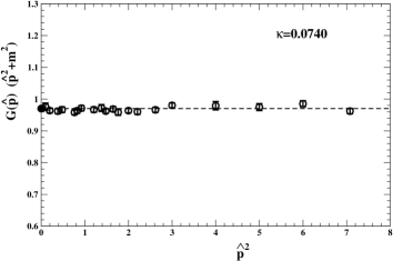
Figure 2: The lattice data from Ref. [10] for the rescaled propagator in the symmetric phase at $\kappa=0.074$, as a function of the lattice momentum squared ${\hat{p}}^{2}$. The fitted mass from high ${\hat{p}}^{2}$, viz. $m_{\rm{latt}}=0.2141\,(28)$, describes the data well, down to ${\hat{p}}=0$.

in the broken-symmetry phase there is a transition between two regimes. As pointed out by Stevenson [33], by rescaling all data with the mass from the higher-momentum fit, the deviations from constancy become highly significant in the $p\to 0$ limit. In Ref. [10] this was checked with a simulation on a large $76^{4}$ lattice; see Figs. 3 and 4.

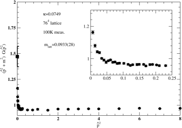
Figure 3: The propagator data from Ref. [10], for $\kappa=0.0749$, rescaled with the lattice mass $M_{H}\equiv m_{\rm{latt}}=0.0933\,(28)$ obtained from the fit to all data with ${\hat{p}}^{2}>0.1$. The peak at $p=0$ is $M^{2}_{H}/m^{2}_{h}=1.47\,(9)$, as computed from the fitted $M_{H}$ and the zero-momentum mass $m_{h}=0.0769\,(8)$.

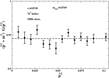
Figure 4: The propagator data from Ref. [10] at $\kappa=0.0749$ for ${\hat{p}}^{2}<0.1$. The lattice data were rescaled here with zero-momentum mass $m_{h}=0.0769\,(8)$.

As such, to obtain a good description of the propagator data in the full momentum region, one had to use a two-mass form [12]

$$G(p)\;\sim\;\frac{1-I(p)}{2}\frac{Z_{h}}{p^{2}+m^{2}_{h}}+\frac{1+I(p)}{2}\frac{Z_{H}}{p^{2}+M^{2}_{H}}\;,$$ (20)

with an interpolating function $I(p)$ that depends on an intermediate momentum scale $p_{0}$ and tends to $+1$ for large $p^{2}\gg p^{2}_{0}$ and to $-1$ when $p^{2}\to 0$. Note that this functional form gives mutually exclusive unit residuals, namely $(1+I(p))/2=1$ where $(1-I(p))/2=0$ and, vice versa, $(1+I(p))/2=0$ where $(1-I(p))/2=1$. Furthermore, extrapolation toward the continuum limit with various lattices was consistent with the expected scaling trend $M^{2}_{H}\sim Lm^{2}_{h}$ from Eq. (14). To this end, from the lattice data for the propagator one extracted a numerical constant $c_{2}$ that determines the logarithmic slope

$$\frac{M^{2}_{H}}{m^{2}_{h}}\Big{|}_{\rm latt}\sim L\,(c_{2})^{-1}\;.$$ (21)

The values of $(c_{2})^{-1/2}=M_{H}\,m_{h}^{-1}\,L^{-1/2}$ are reported in Table 1 and, given their consistency, lead to a final

Table 1: For various values of the hopping parameter $\kappa$ of the 4D Ising model, we report the mass $M_{H}$ obtained from the higher-momentum propagator data by various authors and the zero-momentum $m_{h}$; see Ref. [10]. For $\kappa=0.0749$ the three values of $M_{H}$ refer to high-momentum fits for ${\hat{p}}^{2}>0.1$, ${\hat{p}}^{2}>0.15$ and ${\hat{p}}^{2}>0.2$ respectively on the $76^{4}$ lattice of ref.[10]. The lattice cutoff $\Lambda_{L}\sim\pi/a$ and all masses are in units of the inverse lattice spacing $a$. In the last column, we report the combination $(c_{2})^{-1/2}=M_{H}\,(m_{h})^{-1}\,L^{-1/2}$. The table is adapted from the original table in Ref. [10].

$\kappa$	$M_{H}$	$(m_{h})^{-1}$	$[\ln(\Lambda_{L}/M_{H})]^{-1/2}$	$(c_{2})^{-1/2}$
0.07512	0.2062(41)	5.386(23)	0.606(2)	0.673(14)
0.0751	$\sim 0.200$	5.568(16)	$\sim 0.603$	$\sim 0.671$
0.07504	0.1723(34)	6.636(32)	0.587(2)	0.671(14)
0.0749	0.0933(28)	13.00(14)	0.533(2)	0.647(22)
0.0749	0.096(4)	13.00(14)	0.535(3)	0.668(31)
0.0749	0.100(6)	13.00(14)	0.538(4)	0.699(42)

determination

$$\frac{1}{\sqrt{c_{2}}}\;=\;0.67\pm 0.01~{}({\rm stat})\pm 0.02~{}({\rm sys})\;.$$ (22)

Therefore, in order to estimate $M_{H}$, the following strategy was adopted:

1. First, one used the Gaussian-approximation relation (valid in the whole range of $m_{\Phi}$ and not just for $m_{\Phi}=0$)

   $$M^{2}_{H}\;=\;\frac{\lambda}{3}\;~{}\;\phi_{v}^{2}\;.$$ (23)

2. Second, the rescaling $Z_{\phi}=\phi_{v}^{2}/v^{2}=M^{2}_{H}/m^{2}_{h}$ was extracted from the lattice data for the propagator, yielding

   $$\phi^{2}_{v}\;\sim\;v^{2}\,L\,(c_{2})^{-1}\;.$$ (24)

3. Finally, in Eq. (23) one used the leading-log relation

   $$\lambda\;\sim\;\frac{16\pi^{2}}{3}\,L^{-1}\;.$$ (25)

This way, the constant $K$ was determined as

$$K=\frac{4\pi}{3}\,(c_{2})^{-1/2}=2.80\pm 0.04\,({\rm stat})\pm 0.08\,({\rm sys})\;,$$ (26)

(or $K\sim 8\pi/9$), so that for $v\sim$ 246 GeV one finds

$$(M_{H})^{\rm Theor}=Kv=690\pm 10\,({\rm stat})\pm 20\,({\rm sys})\,{\rm GeV}.$$ (27)

This numerical estimate represents on the one hand a definite prediction to be compared to experiment. On the other hand, it helps to clarify the relation to the more conventional picture of a cutoff theory with only $m_{h}$. To this end, we note that, from the relations in Eq. (14), one finds $m_{h}\ll M_{H}$ for very large $\Lambda$. But $M_{H}$ is independent of $\Lambda$, so that by decreasing $\Lambda$ and so increasing the lower mass, the latter approaches its maximun value $(m_{h})^{\rm max}\sim M_{H}$ when the cutoff $\Lambda$ becomes a few times $M_{H}$. Therefore, this maximum value corresponds to

$$(m_{h})^{\rm max}\!\!\sim\!\!(M_{H})^{\rm Theor}\!=\!690\pm 10\,({\rm stat})\pm 20\,({\rm sys})\,{\rm GeV},$$ (28)

in good agreement with the old theoretical upper bound $(m_{h})^{\rm max}=$ 670 (80) GeV (see Lang’s complete review [34]). However, in the real world $m_{h}=125$ GeV, so that, if there is a second resonance with $M_{H}\sim 700$ GeV, $\Lambda$ should be extremely large.

3 Basic phenomenology of the second resonance

Before exploring the possible implications for the full Standard Model, let us first summarise the picture of SSB in $\Phi^{4}$ theory presented in the previous section:

1. Lattice simulations in the Ising limit support a view of SSB as a weak first-order phase transition. This is relevant for the Standard Model, because the Ising limit, with a lattice coupling at the Landau pole, is known to saturate the triviality bound in $\Phi^{4}$. Namely, for any non-zero renormalised coupling, it represents the best approximation to the continuum limit.

2. This weak first-order scenario is also recovered in those known approximations where the effective potential has the same basic structure of a classical background plus a ZPE of free-field-like fluctuations with some $\phi$-dependent mass. In this sense, there is consistency with the basic “triviality” property of $\Phi^{4}$ theories in 4D.

3. These known approximations to the effective potential predict the same pattern of scales in Eq. (14). As a consequence, the mass parameter $M_{H}$, associated with the ZPEs that determine the potential depth, is much larger than the mass parameter $m_{h}$ defined by the quadratic shape of the effective potential at the minimum. The scalar propagator should thus deviate from a standard one-mass structure.

4. Lattice simulations of the propagator confirm the existence of these deviations, because a good description of the data in the whole momentum range requires a two-mass interpolating form as in Eq. (20). Crucially, the data are consistent with the expected scaling trend $M^{2}_{H}\sim Lm^{2}_{h}$ in Eq. (14).

5. By combining analytical and numerical relations, the second mass scale $M_{H}$ can be estimated to be about 700 GeV.

We believe that these five points a)–e) represent a consistent description of SSB in a $\Phi^{4}$ theory. At the same time, given the large value $M_{H}\sim$ 700 GeV, including the ZPEs of all known gauge and fermion fields at the Fermi scale would represent a small radiative correction. As in the early days of the Standard Model, one could thus adopt the perspective of explaining SSB within the pure scalar sector and restrict the analysis to a region around the Fermi scale that is not much larger than a few TeV. Then, once $\lambda^{\rm(p)}(v)$ and $\lambda(v)$ have the same value as in Eq. (5), their different evolution at asymptotically large energies should remain unobservable. Checking our proposed mechanism for SSB then requires the observation of a second resonance and analysing its phenomenology.

As for the relevant phenomenology, a Higgs resonance with mass $M_{H}\sim$ 700 GeV is usually believed to be a broad resonance due to strong interactions in the scalar sectors. This belief derives from two arguments, namely the definition of $M_{H}$ from the quadratic shape of the potential, which is not valid in our case, and the tree-level calculation of longitudinal $WW$ scattering. Then, at high energies, due to an incomplete cancelation of graphs, the mass in the scalar propagator is effectively promoted to a coupling constant. For the sake of clarity, we shall consider this second argument in a high-energy regime where the Higgs-field propagator is dominated by the second resonance, as in the standard one-pole calculations. From the tree-level expression reported by Veltman and Yndurain [35], we then get

$$A_{\rm ww}\;=\;\frac{g^{2}}{4M^{2}_{w}}\left[a_{\rm tree}(s)+a_{\rm tree}(t)+a_{\rm tree}(u)\right]\;,$$ (29)

where $g=g_{\rm gauge}$, $M^{2}_{w}=g^{2}v^{2}/4$, and the tree-level amplitude is

$$a_{\rm tree}(x)\;=\;x+\frac{x^{2}}{M^{2}_{H}-x}\;.$$ (30)

Therefore, for $|x|\gg M^{2}_{H}$ as in a multi-TeV collider, the tree-level amplitude is governed by a contact coupling

$$\lambda_{0}\;=\;\frac{3M^{2}_{H}}{v^{2}}$$ (31)

as in a pure $\Phi^{4}$ theory. Notice that the tree-level calculation yields $\lambda_{0}$, while, from the $\Phi^{4}$ effective potential, we found

$$\lambda(v)\;=\;\frac{3M^{2}_{H}}{\phi^{2}_{v}}\;=\;\frac{3m^{2}_{h}}{v^{2}}\;=\;\frac{m^{2}_{h}}{M^{2}_{H}}\,\lambda_{0}\;,$$ (32)

which derives from the assumed “triviality” of the theory. To understand the replacement, let us recall the precise formulation of the Equivalence Theorem given by Bagger and Schmidt [36]. This is a non-perturbative statement in the sense that it holds to all orders in the scalar self-interactions, up to $\mathcal{O}(g^{2})$ corrections. One then expects that resumming all higher-order graphs in longitudinal $WW$ scattering gives the same result as in a pure $\Phi^{4}$ theory, if Goldstone $\chi\chi$ diagrams are resummed with the $\beta-$function of $\Phi^{4}$. This resummation, for $M_{H}\sim 700$ GeV, means replacing $\lambda_{0}\sim 24$ with $\lambda(v)\sim 0.78$. For this reason, no large effect proportional to $\lambda_{0}$ should be visible at the Fermi scale or at the relatively nearby energies of a multi-TeV collider (where both $\lambda(E)$ and $\lambda^{\rm(p)}(E)$ differ from their common value 0.78 by negligible terms). In this sense, the second resonance will mimic a conventional Higgs particle of mass $M_{H}$, provided the cutoff-independent ratios $M^{2}_{H}/v$ and $(M_{H}/v)^{2}$, in the three-point and four-point scalar couplings, respectively, are rescaled as follows [37]:

$$\frac{M^{2}_{H}}{2v}\;\to\;\epsilon_{1}\,\frac{M^{2}_{H}}{2v}\;,\;\;\;\frac{M^{2}_{H}}{8v^{2}}\;\to\;\epsilon_{2}\,\frac{M^{2}_{H}}{8v^{2}}\;,$$ (33)

with

$$\epsilon^{2}_{1}\;=\;\epsilon_{2}\equiv\frac{1}{Z_{\phi}}\;=\;\frac{m^{2}_{h}}{M^{2}_{H}}\;.$$ (34)

We can thus predict $\Gamma(H\to WW)$ and $\Gamma(H\to ZZ)$ from their conventional values by replacing the large width $\Gamma^{\rm conv}(H\to WW+ZZ)\sim G_{F}M^{3}_{H}$ with the corresponding value $\Gamma(H\to WW+ZZ)\sim M_{H}(G_{F}m^{2}_{h})$, which retains the same phase-space factor $M_{H}$, but has a coupling rescaled by the small ratio $m^{2}_{h}/M^{2}_{H}\sim 0.032$. In a first estimate, just to display the large renormalisation effect, we can retain the lowest-order values [38] and (for $M_{H}\sim 700$ GeV) we find

$$\Gamma(H\to ZZ)\!\! \!\!\sim \frac{M_{H}}{700\;{\rm GeV}}\,\frac{m^{2}_{h}}{(700\;{\rm GeV})^{2}}\,50.1\;{\rm GeV}\sim$$ (35)

$$\frac{M_{H}}{700\;{\rm GeV}}\,1.6\;{\rm GeV}$$

and

$$\Gamma(H\to WW) \sim \frac{M_{H}}{700~{}{\rm GeV}}\,\frac{m^{2}_{h}}{(700~{}{\rm GeV})^{2}}\;\times$$ (36)

$$102.6~{}{\rm GeV}\frac{M_{H}}{700\;{\rm GeV}}\,3.3\;{\rm GeV}\;.$$

On the other hand, the decays into fermions, gluons, photons, …should be unchanged, yielding

$$\begin{array}[]{c}\Gamma(H\to{\rm fermions+gluons+photons+\ldots})\;\sim\\[2.84526pt] \displaystyle\frac{M_{H}}{700~{}{\rm GeV}}\,27\;{\rm GeV}\;.\end{array}$$ (37)

Therefore, for $M_{H}=660\div 720$ GeV, one would expect a total width $\Gamma_{H}\equiv\Gamma(H\to all)=30\div 33$ GeV. However, this estimate does not account for the new contributions from the decays of the heavier resonance into the lower-mass state at 125 GeV. These include the two-body decay $H\to hh$, the three-body processes $H\to hhh$, $H\to hZZ$, $H\to hW^{+}W^{-}$, and higher-multiplicity final states allowed by phase space. For this reason, the above value $\Gamma_{H}\sim 30$ GeV should likely represent a lower bound. It is not so simple to evaluate the new contributions to the total decay width, because of the $h$-$H$ overlapping and possible mixing, which make this a non-perturbative problem. Nevertheless, on the one hand, we will show in Sec. 4 that some LHC data can be used to experimentally constrain the main branching ratio $B(H\to hh)<0.12\div 0.15$ at the 95% confidence level, thus leading to $\Gamma_{H}<38~{}{\rm GeV}$. On the other hand, in Sec. 5 we will outline a method similar to the RSE approach [45, 46, 47], used in analogous problems with meson resonances, which could be useful if, on the contrary, the width would turn out to be smaller than expected.

Given this theoretical uncertainty, in Ref. [16] a test in the “golden” four-lepton channel was considered which does not require knowledge of the total width and only relies on two assumptions:

1. A resonant four-lepton production through the chain $H\to ZZ\to 4l$   ($l=e,\mu$);

2. An estimate of $\Gamma(H\to ZZ)$ from Eq. (35).

Therefore, by defining $\gamma_{H}=\Gamma_{H}/M_{H}$, we find a fraction

$$B(H\to ZZ) = \frac{\Gamma(H\to ZZ)}{\Gamma_{H}}\;\sim\;$$ (38)

$$\frac{1}{\gamma_{H}}\,\frac{50.1}{700}\,\frac{m^{2}_{h}}{(700\,{\rm GeV})^{2}}$$

that will be replaced in the cross section approximated by the on-shell branching ratios

$$\sigma_{R}(pp\to H\to 4l) \sim \sigma(pp\to H)\,B(H\to ZZ)\times$$ (39)

$$4B^{2}(Z\to l^{+}l^{-})\;.$$

This should be a good approximation for a relatively narrow resonance, so that one predicts a particular correlation

$$\gamma_{H}\,\sigma_{R}(pp\to H\to 4l) \sim \sigma(pp\to H)\,\frac{50.1}{700}\times$$ (40)

$$\frac{m^{2}_{h}}{(700~{}{\rm GeV})^{2}}\,4B^{2}(Z\to l^{+}l^{-})\;,$$

which can be compared to the LHC data.

Since $4B^{2}(Z\to l^{+}l^{-})\sim 0.0045$, in order to check our prediction the last needed ingredient is the total production cross section $\sigma(pp\to H)$, which in our case will mainly result from the gluon-gluon Fusion (ggF) process. In fact, the other production mechanism through Vector-Boson Fusion (VBF) plays no role here, since the large coupling to longitudinal $W$s and $Z$s is suppressed by the small coefficient $m^{2}_{h}/M^{2}_{H}\sim 0.032$. As a consequence, the traditionally large VBF cross section $\sigma^{\rm VBF}(pp\to H)\sim 300$ fb is reduced to about 10 fb and can be safely neglected in comparison with the pure ggF contributions of $\mathcal{O}(10^{3})$ fb. Indeed, for $pp$ collisions at 13 TeV and with a typical $\pm 15\%$ uncertainty (due to the parton distributions, the choice of $\mu$ in $\alpha_{s}(\mu)$, and other effects), we will adopt the value [48] $\sigma^{\rm ggF}(pp\to H)=1090\>(170)$ fb, which also accounts for the possible mass range $M_{H}=660\div 700$ GeV.

In conclusion, for $m_{h}=$ 125 GeV, one obtains a prediction that, for a not too large $\gamma_{H}$ where Eq. (39) starts to lose validity, is formally insensitive to the value of $\Gamma_{H}$ and can be directly compared to the four-lepton data

$$\left[\gamma_{H}\,\sigma_{R}(pp\to H\to 4l)\right]^{\rm Theor}\sim(0.011\pm 0.002)\,{\rm fb}\,.$$ (41)

4 Some experimental signals from LHC

To test our definite prediction $(M_{H})^{\rm Theor}=690\pm 10\,(\mbox{stat})\pm 20\,(\mbox{sys})$ GeV, one should look for deviations from the background nearby. This means that local deviations should not be downgraded by the so called “look elsewhere” effect. At the same time, given the present energy and luminosity of LHC, the second resonance, if there, is too heavy to be seen unambiguously in all possible channels. In this sense, one should remember the $h(125)$ discovery, which, at the beginning, was producing no signals in the important $b\bar{b}$ and $\tau^{+}\tau^{-}$ channels.

After this premise, given the expected large branching ratio $B(H\to t\bar{t})=(75\div 80)\%$, the most natural place to look for the new resonance would be in the $t\bar{t}$ channel. However, in the relevant region of invariant mass $m(t\bar{t})=620\div 820$ GeV, CMS measurements [49] give a background cross section $\sigma(pp\to t\bar{t})=107\pm 7.6$ pb that is about 100 times larger than the expected signal $\sigma(pp\to H\to t\bar{t})\lesssim 1$ pb.. For this reason, in Refs. [16, 17, 18, 19] the phenomenological analysis was focused on available channels with relatively smaller background, namely:

1. ATLAS ggF-like four-lepton events;

2. ATLAS high-mass inclusive $\gamma\gamma$ events;

3. ATLAS and CMS $(b\bar{b}+\gamma\gamma)$ events;

4. CMS $\gamma\gamma$ events produced in $pp$ diffractive scattering.

4.1 The ATLAS ggF-like 4-lepton events

As a first sample, let us focus on the ATLAS charged four-lepton channel [52]. In the search for a heavy scalar resonance $H$, decaying through the chain $H\to ZZ\to 4l$, the ATLAS experiment has performed a sophisticated analysis in which the four-lepton events, depending on their topology, are divided into ggF-like and VBF-like events. By expecting our second resonance to be produced through gluon-gluon fusion, we have considered the ggF-like category, which, depending on the degree of contamination with the background, is further divided into four mutually exclusive subcategories: ggF-high-4$\mu$, ggF-high-2e2$\mu$, ggF-high-4e, ggF-low.

The only sample which is homogeneous from the point of view of the selection and has a sufficient statistics is the ggF-low category which contains a mixture of all three final states. We understand that the ggF-low sample is certainly less pure as compared to the ggF-high samples, and it is true that it includes the dominating contribution from other sources of non-resonant $ZZ$ events. On the other hand, this background was, according to ATLAS, carefully evaluated with a total quoted (statistical + systematical) uncertainty of less than 5% in the relevant region. As such, there is no reason not to consider it as our best estimate and safely compare background and observed events. Since in the region of invariant mass around 700 GeV the energy resolution of these events varies considerably, it is natural to adopt a large-bin visualization to avoid spurious fluctuations between adjacent bins. The numbers of events for this category are shown in Table 2, together with the background estimated by ATLAS [52].

Table 2: For a luminosity of 139 fb^-1, we report the observed ATLAS [52] ggF-low events $\rm{N}_{\rm EXP}(E)$ and the corresponding estimated background $\rm{N}_{\rm B}(E)$ in the range of invariant mass $m(4l)=E=530\div 830$ GeV. In view of the considerable difference in the energy resolution of the various types of four-lepton events, to avoid spurious migrations between neighbouring bins, we have grouped the data into larger bins of 60 GeV, centred at 560, 620, 680, 740, and 800 GeV. These correspond to the 10 bins of 30 GeV, from $545\,(15)$ GeV to $815\,(15)$ GeV; see Ref. [52]. In this energy range, the uncertainties in the background are below 5% and have been neglected. The statistical errors of $\rm{N}_{\rm EXP}(E)$ are not reported by ATLAS and will be assumed to be given by $\sqrt{\rm{N}_{\rm EXP}}$, as for a Poisson distribution.

$\rm E$ [GeV]	$\rm{N}_{\rm EXP}(E)$	$\rm{N}_{\rm B}(E)$	$\rm{N}_{\rm EXP}(E)-\rm{N}_{\rm B}(E)$
$560\,(30)$	38$\pm 6.16$	32.0	$6.00\pm 6.16$
$620\,(30)$	25$\pm 5.00$	20.0	$5.00\pm 5.00$
$680\,(30)$	26$\pm 5.10$	13.04	$12.96\pm 5.10$
$740\,(30)$	3$\pm 1.73$	8.71	$-5.71\pm 1.73$
$800\,(30)$	7$\pm 2.64$	5.97	$1.03\pm 2.64$

From this comparison, one finds a considerable excess over the background, in the bin centred around 680 GeV, followed by a sizable defect in the next bin centred around 740 GeV. The simplest explanation for these two simultaneous features would be the existence of a resonance of mass $M_{H}\sim 700$ GeV which, above the Breit-Wigner peak, produces the characteristic negative-interference pattern proportional to $(M^{2}_{H}-s)$.

To check this idea, we will exploit the basic model where the $ZZ$ pairs, each of which subsequently decaying into a charged $l^{+}l^{-}$ pair, are produced by various mechanisms at the parton level. Depending on the invariant mass of the four final leptons $E\equiv m(4l)$, this gives rise to a smooth distribution of background events $N_{b}(E)$, proportional to a background cross section $\sigma_{b}(E)$.

To describe the effects of a resonance, let us denote by $A_{b}(E)$ the background amplitude, whose squared modulus is proportional to $\sigma_{b}(E)$, and by $A_{R}(E)$ the amplitude describing $ZZ$ production through the intermediate resonance $H$. We thus obtain a total amplitude $A_{T}(E)=A_{b}(E)+A_{R}(E)$, whose square modulus will be proportional to the total cross section. Now, by defining $s=E^{2}$ and introducing the complex resonance mass $M^{2}_{R}=M^{2}_{H}-iM_{H}\Gamma_{H}$ for a relatively narrow resonance, the resonant amplitude can be approximated in terms of some constant $a_{R}$ as

$$A_{R}(E)\;\sim\;\frac{a_{R}}{s-M^{2}_{R}}\;.$$ (42)

Introducing then a (common) phase-space normalisation constant $\xi$ such that $\xi|A_{b}(E)|^{2}=\sigma_{b}(E)$ and $\xi|A_{R}(E)|^{2}=$ $\sigma_{R}(E)$, with

$$\sigma_{R}(E)\;=\;\frac{\xi a^{2}_{R}}{(s-M^{2}_{H})^{2}+(\Gamma_{H}M_{H})^{2}}\;,$$ (43)

the total cross section $\sigma_{T}(E)=\xi|A_{T}(E)|^{2}$ can be conveniently expressed as

$$\sigma_{T}(E) = \sigma_{b}(E)\;+\;\frac{2(M^{2}_{H}-s)\,\Gamma_{H}M_{H}}{(s-M^{2}_{H})^{2}\;+\;(\Gamma_{H}M_{H})^{2}}\times$$ (44)

$$\sqrt{\sigma_{R}\sigma_{b}(E)}\;+\;\frac{(\Gamma_{H}M_{H})^{2}}{(s-M^{2}_{H})^{2}\;+\;(\Gamma_{H}M_{H})^{2}}\,\sigma_{R}\;,$$

where we have introduced the resonance peak cross section at $s=M^{2}_{H}$ defined as $\sigma_{R}=\xi a^{2}_{R}/(M^{2}\Gamma^{2}_{H})$ and assumed positive interference below the peak as suggested by the data.

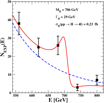
Figure 5: The values $\rm{N}_{\rm EXP}(E)$ in Table 2 for ATLAS [52] data vs. the corresponding $\rm{N}_{\rm TH}(E)$ in Eq. (45) (solid red curve). The resonance parameters are $M_{H}=706$ GeV, $\gamma_{H}=0.041$, $\sigma_{R}=0.23$ fb and the ATLAS background (dashed blue curve) is approximated as $N_{b}(E)=A\times({\rm 710~{}GeV}/E)^{\nu}$, with $A=10.55$ and $\nu=4.72$.

Now, an accurate description of the ATLAS background can be obtained in terms of a power law $N_{b}(E)\sim A\times({\rm 710~{}GeV}/E)^{\nu}$, with $A\sim 10.55$ and $\nu\sim 4.72$. Then, by simple redefinitions, the theoretical number of events can be expressed as

$$N_{TH}(E)\;=\;N_{b}(E)+\frac{P^{2}+2P\,x(E)\,\sqrt{N_{b}(E)}}{\gamma^{2}_{H}+x^{2}(E)}\;,$$ (45)

where $x(E)=(M^{2}_{H}-E^{2})/M^{2}_{H}$, $P\equiv\gamma_{H}\sqrt{N_{R}}$, and $N_{R}=\sigma_{R}\times{\cal A}\times 139$ fb^-1 denotes the extra events at the resonance peak, for an acceptance ${\cal A}$.

As for the acceptance, one can adopt a value ${\cal A}\sim 0.38$ by averaging the two extremes, viz. 0.30 and 0.46, for the ggF-like category of events [52]. As a consequence, the resonance parameters are affected by an additional uncertainty. Nevertheless, to have a first check, in Refs. [18, 19] the experimental number of events given in Table 2 was fitted with Eq. (45). The results were: $M_{H}=706\,(25)$ GeV, $\gamma_{H}=0.041\pm 0.029$ (corresponding to a total width $\Gamma_{H}=29\pm 20$ GeV), and $P=0.14\pm 0.07$. From these numbers one obtains $N_{R}\sim 12^{+15}_{-9}$ and $\sigma_{R}\sim 0.23^{+0.28}_{-0.17}$ fb. The theoretical values are shown in Table 3 and a graphical comparison in Fig. 5.

Table 3: The observed ATLAS [52] ggF-low events and our theoretical prediction in Eq. (45), for $M_{H}=706$ GeV, $\gamma_{H}=0.041$, $P=0.14$.

$\rm E$ [GeV]	$\rm{N}_{\rm EXP}(E)$	$\rm{N}_{\rm TH}(E)$	$\chi^{2}$
$560\,(30)$	38$\pm 6.16$	36.72	0.04
$620\,(30)$	25$\pm 5$	25.66	0.02
$680\,(30)$	26$\pm 5.10$	26.32	0.00
$740\,(30)$	3$\pm 1.73$	3.23	0.02
$800\,(30)$	7$\pm 2.64$	3.87	1.40

The quality of the fit is good, but error bars are large and the test of our picture is not very stringent. Still, with the partial width from Sec. 3, viz. $\Gamma(H\to ZZ)\sim 1.6$ GeV, and fixing $\Gamma_{H}$ to its central value of 29 GeV, we find a branching ratio $B(H\to ZZ)\sim 0.055$ that, for the central value $\sigma^{\rm ggF}(pp\to H)\sim 923$ fb from Ref. [48] at $M_{H}=$ 700 GeV, would imply a theoretical peak cross section $(\sigma_{R})^{\rm theor}=923\times 0.055\times 0.0045\sim 0.23$ fb, which coincides with the central value from our fit. Moreover, from the central values $\langle\sigma_{R}\rangle=0.23$ fb and $\langle\gamma_{H}\rangle=0.041$, we find $\langle\sigma_{R}\rangle\times\langle\gamma_{H}\rangle\sim 0.0093$ fb, in accordance with Eq. (41).

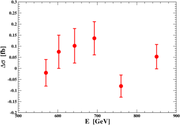
Figure 6: The quantity $\Delta\sigma=(\sigma_{\rm EXP}-{\sigma}_{\rm B})$ reported for each bin in the last column of Table 4, for the ATLAS data of Ref. [53].

Table 4: The observed ATLAS [53] cross section and the estimated background in the range of four-lepton invariant mass $m(4l)\equiv E$ from 555 to 900 GeV. These values have been obtained by multiplying the bin size with the average differential cross sections $\langle(d\sigma/dE)\rangle$, reported for each bin in the companion HEPData file. Besides the non-resonant $gg\to 4l$ process, the background cross section $\sigma_{B}$ contains the dominating contributions from $q\bar{q}\to 4l$ events (as well as from other sources).

.

Bin [GeV]	${\sigma}_{\rm EXP}$ [fb]	$\rm{\sigma}_{\rm B}$ [fb]	$(\sigma_{\rm EXP}-\rm{\sigma}_{\rm B}$) [fb]
555–585	0.252 $\pm 0.056$	$0.272\pm 0.023$	$-0.020\pm 0.060$
585–620	$0.344\pm 0.070$	$0.259\pm 0.021$	$+0.085\pm 0.075$
620–665	$0.356\pm 0.075$	$0.254\pm 0.023$	$+0.102\pm 0.078$
665–720	$0.350\pm 0.073$	$0.214\pm 0.019$	$+0.136\pm 0.075$
720–800	$0.126\pm 0.047$	$0.206\pm 0.018$	$-0.080\pm 0.050$
800–900	$0.205\pm 0.052$	$0.152\pm 0.017$	$+0.053\pm 0.055$

After having recalled this first comparison from Refs. [18, 19], we will now illustrate the indications obtained from the other ATLAS paper [53], in which the differential four-lepton cross section $\langle d\sigma/dE\rangle$, with $E=m(4l)$, is reported in the same energy region. By inspection of Fig. 5 of this Ref. [53], one finds the same type of excess-defect sequence as in Table 2 and so additional support for the idea of a new resonance. To make this clear, the corresponding data are given in Table 4 and displayed in Fig. 6.

Most notably, however, by comparing with Ref. [53] we can also sharpen our analysis. The point is that the background estimated by ATLAS, for the class of ggF-low events considered above, contains more events than those which in principle can interfere with our resonance. In particular, it contains a large contribution from $q\bar{q}\to 4l$ processes. Although the initial state is $pp$ in all cases, our $H$ resonance would mainly be produced through gluon-gluon fusion and therefore, strictly speaking, the interference should only be computed with the non-resonant $gg\to 4l$ background.

Obtaining this refinement is now possible because, in the HEPData file of Ref. [53], the individual contributions to the expected background are reported separately. Denoting by $\rm{\sigma}^{\rm gg}_{\rm B}$ the pure non-resonant $gg\to 4l$ background cross section, we can thus consider a corresponding experimental cross section ${\hat{\sigma}}_{\rm EXP}$ after subtracting preliminarily the “non-ggF” background, i.e.,

$${\hat{\sigma}}_{\rm EXP}\;=\;\sigma_{\rm EXP}-(\rm{\sigma}_{\rm B}-\rm{\sigma}^{\rm gg}_{\rm B})\;.$$ (46)

The corresponding values for these redefined cross sections and background are given in Table 5.

Table 5: The ATLAS [53] experimental cross section ${\hat{\sigma}}_{\rm EXP}$ from Eq. (46) for each energy bin. The two cross sections ${\sigma}_{\rm EXP}$ and $\rm{\sigma}_{\rm B}$ are given in Table 4. The other background cross section $\rm{\sigma}^{\rm gg}_{\rm B}$ only takes into account the non-resonant $gg\to 4l$ process and was computed by multiplying the bin size with the average differential cross section $(d\rm{\sigma}^{\rm gg}_{\rm B}/dE)$ in each bin. The central value of ${\hat{\sigma}}_{\rm EXP}$ in the second column of the $720$–$800$ GeV bin is negative, because the expected background in Table 4, from $q\bar{q}\to 4l$ events (as well as from other sources), is larger than the experimental value itself.

Bin [GeV]	${\hat{\sigma}}_{\rm EXP}$ [fb]	$\rm{\sigma}^{\rm gg}_{\rm B}$ [fb]	$(\hat{\sigma}_{\rm EXP}-\rm{\sigma}^{\rm gg}_{\rm B})$ [fb]
555–585	0.003 $\pm 0.060$	$0.023\pm 0.004$	$-0.020\pm 0.060$
585–620	$0.105\pm 0.073$	$0.020\pm 0.003$	$+0.085\pm 0.075$
620–665	$0.121\pm 0.078$	$0.019\pm 0.003$	$+0.102\pm 0.078$
665–720	$0.152\pm 0.075$	$0.016\pm 0.003$	$+0.136\pm 0.075$
720–800	$-0.067\pm 0.050$	$0.013\pm 0.002$	$-0.080\pm 0.050$
800–900	$0.062\pm 0.055$	$0.009\pm 0.002$	$+0.053\pm 0.055$

Table 6: Comparing the ATLAS [53] cross section of Table 5 with the theoretical Eq. (44) for the optimal set of parameters $M_{H}=677$ GeV, $\Gamma_{H}=21$ GeV, $\sigma_{R}=0.40$ fb.

.

Bin [GeV]	${\hat{\sigma}}_{\rm EXP}$ [fb]	$\sigma_{T}$ [fb]	$\chi^{2}$
555–585	0.003 $\pm 0.060$	0.048	0.56
585–620	$0.105\pm 0.073$	0.056	0.45
620–665	$0.121\pm 0.078$	0.123	0.00
665–720	$0.152\pm 0.075$	0.152	0.00
720–800	$-0.067\pm 0.050$	0.002	1.90
800–900	$0.062\pm 0.055$	0.004	1.11

We then compare the resulting experimental ${\hat{\sigma}}_{\rm EXP}$ with the theoretical $\sigma_{T}$ from Eq. (44), after the identification $\sigma_{b}=\rm{\sigma}^{\rm gg}_{\rm B}$. By parametrising the ATLAS differential background $(d\rm{\sigma}^{\rm gg}_{\rm B}/dE)\sim A\times({\rm 710~{}GeV}/E)^{\nu}$ with $A\sim(2.42\pm 0.18)\times 10^{-4}$ and $\nu\sim 5.24\pm 0.45$, and integrating the various contributions to Eq. (44) within each energy bin, a fit to the data results in $M_{H}=677^{+30}_{-14}$ GeV, $\Gamma_{H}=21^{+28}_{-16}$ GeV, and $\sigma_{R}=0.40^{+0.62}_{-0.34}$ fb. The comparison for the optimal parameters is shown in Table 6.

As in the case of the ggF-low events, the quality of our fit is good, but error bars are large. Still, by restricting ourselves again to the central values, we find a good agreement with our expectations. Indeed, by rescaling the partial width given in Eq. (35) (Sec. 3), from $\Gamma(H\to ZZ)\sim 1.6$ GeV down to 1.55 GeV (for a mass $M_{H}$ from 700 to 677 GeV), and fixing $\Gamma_{H}$ at its central value of 21 GeV, we find a branching ratio $B(H\to ZZ)\sim 0.073$. For the central value $\sigma^{\rm ggF}(pp\to H)\sim 1100$ fb from Ref. [48] at $M_{H}=677$ GeV, this would then imply a theoretical peak cross section $(\sigma_{R})^{\rm Theor}=1100\times 0.073\times 0.0045\sim 0.36$ fb, which only differs by 10% from the central value $\langle\sigma_{R}\rangle=0.40$ fb of our fit. Also, from the central values of the fit $\langle\sigma_{R}\rangle=0.40$ fb and $\langle\gamma_{H}\rangle=0.031$, we find $\langle\sigma_{R}\rangle\times\langle\gamma_{H}\rangle\sim 0.012$ fb, again in good agreement with our Eq. (41).

Let us now summarise these results. By considering the two ATLAS papers [52] and [53], we have found consistent indications of a new resonance in our theoretical mass range $(M_{H})^{\rm Theor}\sim 690\,(30)$ GeV. In particular, by comparing with the cross-section data of Ref. [53], we have identified more precisely the non-resonant background $gg\to 4l$, which can interfere with a second resonance $H$ produced mainly via gluon-gluon fusion. In this sense, the determinations obtained with our Eq. (44) are now more accurate, from a theoretical point of view. In practice, there is not much difference with the previous analysis [18, 19] based on the ggF-low events of Ref. [52]. Indeed, the two mass values $(M_{H})^{\rm EXP}=677^{+30}_{-14}$ GeV vs. $(M_{H})^{\rm EXP}=706\,(25)$ GeV [18, 19] and decay widths $\Gamma_{H}=21^{+28}_{-16}$ GeV vs. $\Gamma_{H}=29\pm 20$ GeV [18, 19], are compatible within their rather large experimental uncertainties. Most notably, our crucial correlation in Eq. (41) is well reproduced by the central values of the fits to the two date sets.

4.2 The ATLAS high-mass $\gamma\gamma$ events

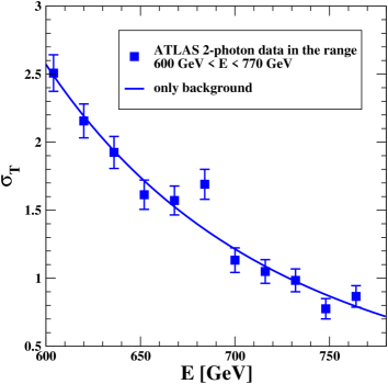
Figure 7: The fit with Eq. (44) and $\sigma_{R}=0$ to the ATLAS [53] data in Table 5, converted to cross sections in fb. The chi-squared value is $\chi^{2}=14$, with the background parameters $A=1.35$ fb and $\nu=4.87$.

Table 7: The ATLAS [54] number of events $N=N(\gamma\gamma)$, in bins of 16 GeV and for a luminosity of 139 fb^-1, in the range of invariant mass $\mu=\mu(\gamma\gamma)=600\div 770$ GeV. These values were extracted from Fig. 3 of Ref. [54], because the corresponding numbers are not reported in the companion HEPData file. In the fits, statistical errors were assumed to be given by $\sqrt{N}$, as for a Poisson distribution.

$\mu$	604	620	636	652	668	684	700	716	732	748	764
$N$	349	300	267	224	218	235	157	146	137	108	120

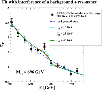
Figure 8: Three fits with Eq. (44) to the ATLAS [53] data in Table 5, converted to cross sections in fb. The $\chi^{2}$ values are 7.5, 8.8, and 10.2, for $\Gamma_{H}=15$, 25, and 35 GeV, respectively.

Searching for other signals, in Refs. [18, 19] one considered the distribution of the inclusive diphoton production by ATLAS [54] in the range of invariant mass $600\div 770$ GeV. The corresponding entries in Table 7 were extracted from Fig. 3 of Ref. [54], because the numerical values are not reported in the companion HEPData file. By parametrising the background with a power-law form $\sigma_{B}(E)\sim A\times 685\,({\rm GeV}/E)^{\nu}$, doing a fit to the data in Table 4 gives a good description of all data points with the exception of a sizable excess at 684 GeV (estimated by ATLAS to have a local significance of more than $3\sigma$); see Fig. 7. This illustrates how a relatively narrow resonance might remain hidden behind a large background almost everywhere, the main signal being just a small interference effect. For this reason, with the exception of the mass $M_{H}=696\,(13)$ GeV, the resonance parameters are determined only very poorly. As for the total width, one finds $\Gamma_{H}=15^{+30}_{-13}$ GeV, which is consistent with the other loose determination $\Gamma_{H}=21^{+28}_{-16}$ GeV from the four-lepton data. In Fig. 8 we show three fits with Eq. (44), viz. for $\Gamma_{H}=15$, 25, and 35 GeV. The widths vary substantially, but the curves cross the background at the same point $M_{H}=696$ GeV where the interference vanishes. Concerning the peak cross section $\sigma_{R}=\sigma_{R}(pp\to H\to\gamma\gamma)$, the fit produces $\sigma_{R}=0.025^{+0.055}_{-0.023}$ fb, with central value $\sqrt{\sigma_{R}\,\sigma_{B}(684)}\sim 0.18$ fb or about $+26$ events. To have an idea, for $M_{H}\sim 700$ GeV, $\Gamma_{H}\sim 29$ GeV and $\sigma(pp\to H)\sim 1$ pb, the partial width $\Gamma(H\to\gamma\gamma)\sim 29$ keV of Ref. [38] implies $B(H\to\gamma\gamma)\sim 1\times 10^{-6}$ and a peak cross section $\sigma_{R}(pp\to H\to\gamma\gamma)\sim 0.001$ fb. Instead, with a larger two-photon width (see footnote 7) one could start to approach the lower band of the fit.

In conclusion, the localised $3\sigma$ excess at 684 GeV admits two different interpretations:

1. a statistical fluctuation above a pure background, see Fig. 7;

2. the signal of a heavy, relatively narrow resonance, see Fig. 8.

4.3 ATLAS and CMS $(b\bar{b}+\gamma\gamma)$ events

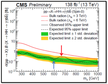
Figure 9: Expected and observed 95% upper limit for the cross section $\sigma(pp\to X\to h(125)h(125)\to b\bar{b}+\gamma\gamma)$ observed by the CMS Collaboration [55].

The ATLAS and CMS Collaborations have also searched for new resonances decaying, through a pair of $h=h(125)$ scalars, into the peculiar final state made up of a $b\bar{b}$ quark pair and a $\gamma\gamma$ pair. In particular, in Ref. [55] the cross section for the full process

$$\sigma({\rm full})\;=\;\sigma(pp\to X\to hh\to b\bar{b}+\gamma\gamma)$$ (47)

was considered. For a spin-zero resonance, the 95$\%$ upper limit $\sigma({\rm full})<0.16$ fb, for an invariant mass of 600 GeV, was found to increase by about a factor of two, up to $\sigma({\rm full})<0.30$ fb, on a plateau of $650\div 700$ GeV and then to decrease for larger energies; see Fig. 9.

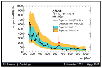
Figure 10: Expected and observed 95$\%$ upper limit for the cross section $\sigma(pp\to X\to h(125)h(125))$ extracted by ATLAS [56] from the final state $(b\bar{b}+\gamma\gamma)$. The figure is taken from the talk given by Bill Balunas at “Higgs 2022” and is the same as Fig. 15 in Ref. [56].

The local statistical significance is modest, about $1.6\sigma$, but the relevant mass region $M_{X}\sim 675\,(25)$ GeV is precise and agrees well with our prediction. Interestingly, if the cross section is approximated as

$$\sigma({\rm full}) \sim \sigma(pp\to H)\>B(H\to hh)\;\times$$ (48)

$$2B(h\to b\bar{b})\>B(h\to\gamma\gamma)\;,$$

the CMS 95$\%$ upper bound $\sigma({\rm full})<0.30$ fb, for $\sigma(pp\to H)\sim$ 1 pb, becomes an upper bound $B(H\to hh)<$ 0.12. In view of the mentioned non-perturbative nature of the decay process $H\to hh$, this represents a precious indication.

The analogous ATLAS plot is shown in Fig. 10 (which is the same as Fig. 15 of the ATLAS paper Ref. [56]). Again, one finds a modest $1.2\sigma$ excess at $650\,(25)$ GeV, followed immediately by a $1.4\sigma$ defect, which could be indicative of a negative above-peak $(M^{2}_{H}-s)$ interference effect of the same type as found in the ATLAS four-lepton data. From the observed value $\sigma(pp\to H\to hh)<150$ fb, this yields $B(H\to hh)<0.15$, so consistent with the CMS determination. Since the three-body decays $H\to hhh$, $H\to hW^{+}W^{-}$, and $H\to hZZ$ should only give a modest contribution to the total width, from the estimates in Sec. 3 we would then deduce $\Gamma_{H}<38$ GeV.

4.4 CMS $\gamma\gamma$ events produced in $pp$ diffractive scattering

Finally, the CMS and TOTEM Collaborations have been searching for high-mass photon pairs produced in $pp$ diffractive scattering, i.e., when both final protons are tagged and have large $x_{F}$. For our purpose, the relevant information is contained in Fig. 11, taken from the CMS report Ref. [57]. In the range of invariant mass $650\,(40)$ GeV and for a statistics of 102.7 fb^-1, the observed number of $\gamma\gamma$ events is $N_{\rm obs}\sim 76\,(9)$, to be compared with an estimated background $N_{\rm B}\sim 40\,(9)$, which is quoted as being the best estimate by CMS. In the most conservative case, namely $N_{\rm B}=49$, this is a local $3\sigma$ effect and the only statistically significant excess in the plot.

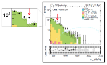
Figure 11: The number of $\gamma\gamma$ events produced in $pp$ diffractive scattering, as reported by CMS [57]. In the range $650\,(40)$ GeV, the observed number was $N_{\rm obs}\sim 76\,(9)$, to be compared to an estimated background $N_{\rm B}\sim 40\,(9)$.

4.5 Experimental summary

Let us finally summarise our review of LHC data:

1. The ATLAS ggF-like four-lepton events in Table 2 show deviations from the background with a definite excess-defect sequence, which could indicate the presence of a resonance. The same pattern is also visible in the ATLAS data for the corresponding differential cross section; see Fig. 5 of Ref. [53] and the corresponding integrated cross sections in Tables 4 and 5. From the last column of these Tables, the combined statistical significance of the observed deviations can be estimated at the $3\sigma$ level. A fit with Eq. (44) gives a good description of the data for a resonance mass $M_{H}=677^{+30}_{-14}$ GeV; see Table 6.

2. Observing the $+3\sigma$ excess at $684\,(16)$ GeV in the inclusive ATLAS $\gamma\gamma$ events, a fit to these data was performed in Refs. [18, 19]. The resulting mass was $M_{H}=696\,(13)$ GeV.
   Furthermore, one should note:

3. The overall $+2\sigma$ effect in the ($b\bar{b}+\gamma\gamma)$ channel, obtained by combining the excess of events observed by ATLAS at $650\,(25)$ GeV and the corresponding excess observed by CMS at $675\,(25)$ GeV.

4. The $+3\sigma$ excess at $650\,(40)$ GeV in the distribution of CMS-TOTEM $\gamma\gamma$ events produced in $pp$ diffractive scattering.

Since the above determinations i)-iv) are well aligned within the uncertainties, one can try to combine the mass values by obtaining $(M_{H})^{\rm comb}\sim 682\,(10)$ GeV, in very good agreement with our expectation $(M_{H})^{\rm Theor}=690\pm 10\,\mbox{(stat)}\pm 20\,\mbox{(sys)}$ GeV. We emphasise again that, when comparing with a definite prediction, one should look for deviations from the background nearby, so that local significance is not downgraded by the so called “look elsewhere” effect. Therefore, since the correlation of the above measurements is small, one could also argue that the combined statistical evidence for a new resonance in the expected mass range is close to (if not above) the traditional $5\sigma$ level. Certainly, one can conclude that the present situation is unstable and could soon be resolved with two still missing sets of RUN2 data, namely

1. the full CMS charged 4-lepton events;

2. the full CMS inclusive high-mass $\gamma\gamma$ events.

By adding these two sets of data, the present non-negligible statistical significance could become an important new discovery. In view of these possible future developments, we will illustrate in the following Sec. 5 the basic ingredients of a coupled-channel calculation that could be useful to further refine the theoretical predictions for the mass and width of the hypothetical new resonance, when interacting with the gauge and fermion sectors of the Standard Model.

5 Unitarity constraints from coupled-channel calculations

Our estimate $(M_{H})^{\rm Theor}$ = 690 $\pm$10 (stat) $\pm$20 (sys) GeV was obtained by combining analytical and numerical results in a pure $\Phi^{4}$ theory. In this sense, this mass value should be considered a “bare” mass that would become the physical mass, to be compared to experiment, after including the interactions with the gauge and fermion fields. For this reason, it is remarkable that the phenomenological analysis illustrated in Sec. 4 suggests a new resonance precisely in the expected region of this bare mass.

As for the total decay width, we started from the standard calculations for a single Higgs particle of mass $M_{H}\sim$ 700 GeV, by taking into account the strong renormalisation of the conventional large widths into longitudinal $W$s by a factor $(125/700)^{2}\sim$ 0.032. This suppression leads to the estimates in Eqs. (35,36) and to the precise correlation in the four-lepton channel in Eq. (41), which, within the large uncertainties of the fit to the ATLAS four-lepton data, is reproduced by the central values $\langle\sigma_{R}(pp\to H\to 4l)\rangle\sim 0.40$ fb and $\langle\gamma_{H}\rangle\sim 0.031$. If checked to high accuracy with future data, this correlation would imply that, indeed, the new resonance is the second resonance of the Higgs field.

Still Eq. (41) is, to a large extent, independent of the total width. Our expectation $\Gamma^{\rm Theor}(H\to all)=30\div 38$ GeV is consistent with the very loose determinations obtained from the fit to the ATLAS four-lepton and $\gamma\gamma$ events. However, with more precise measurements, things could change significantly. To this end, let us consider the following hypothetical experimental values: $(M_{H})^{\rm exp}=700\,(10)$ GeV, $\Gamma^{\rm exp}(H\to all)=22\,(3)$ GeV, and $\sigma_{R}=[\sigma_{R}(pp\to H\to 4l)]^{\rm exp}=0.33\,(5)$ fb. These values would imply a correlation $[\gamma_{H}\times\sigma_{R}]^{\rm exp}=0.010\pm 0.002$, in excellent agreement with Eq. (41), and thus with Eqs. (35,36). But the total width would lie at three-sigma from the expected theoretical value $\Gamma^{\rm Theor}(H\to all)\sim 32$ GeV of Sec. 3. Actually, the discrepancy would be even worse, because the opening of new channels related to $H$ decays into the low-mass state $h(125)$, such as $H\to hh$, should further increase the width up to $\Gamma_{H}\lesssim 38$ GeV. Then, the most natural explanation would consist in a substantial defect in the main partial width $\Gamma(H\to t\bar{t})$. Here, for $m_{t}\sim 173$ GeV one has the lowest-order estimate

$$\Gamma^{\rm LO}(H\to t\bar{t})=\frac{3M_{H}}{8\pi}\frac{m^{2}_{t}}{v^{2}}\!\!\left[1-4\frac{m^{2}_{t}}{M^{2}_{H}}\right]^{3/2}\!\!\!\sim 27.1\,{\rm GeV},$$ (49)

very close to the full value $\Gamma(H\!\to\!t\bar{t})\!\sim\!27.5$ GeV in Ref. [39].

Differently from the more common situation where a decay width turns out to be larger than expected, which suggests the presence of new final states, the presence of a substantial defect could indicate the suppression produced by the unitarity constraints in the presence of several competing decay channels. This problem can be addressed in a coupled-channel analysis such as the so-called Resonance-Spectrum-Expansion (RSE) model. It was developed in Ref. [45, 46, 47] as a momentum-space version of a much earlier [59, 60] coupled-channel model for unquenched meson spectroscopy formulated in coordinate space, which accounts for surprisingly large dynamical effects of strong decay on the spectra.

In Subsec. 5.1 the RSE model is briefly revisited and in Subsec. 5.2 its possible application to a heavy-Higgs system is sketched.

5.1 RSE model for non-exotic meson-meson scattering

The RSE model is a very efficient multichannel formalism that guarantees $S$-matrix unitarity and analyticity in a non-perturbative description of non-exotic meson resonances and bound states as quark-antiquark ($q\bar{q}$) systems coupled to a variety of meson-meson ($MM$) decay channels with the same quantum numbers. Transitions between the $q\bar{q}$ and $MM$ sectors proceed via the creation or annihilation of a new $q\bar{q}$ pair with vacuum quantum numbers and so in a ${}^{3\!}P_{0}$ state. Thus, the off-energy-shell RSE $T$-matrix, graphically depicted [46] in Fig. 12,

Figure 12: Graphical depiction of RSE $T$-matrix for non-exotic two-meson scattering.

describes an incoming pair of mesons that at a ${}^{3\!}P_{0}$ annihilation vertex couple to an intermediate quark-antiquark state propagating in the $s$-channel and then, via a ${}^{3\!}P_{0}$ creation vertex, give rise to an outgoing — possibly different — pair of mesons. The $T$-matrix in Fig. 12 clearly amounts to a Born term plus an infinite set of bubble diagrams. As for the intermediate state, a whole tower of bare $q\bar{q}$ levels with the same quantum numbers is taken. The vertices are modeled by spherical Bessel functions, which are the Fourier transforms of a spherical $\delta$ function, thus mimicking string breaking at a certain interquark distance. Due to the separability of the effective $MM$ interaction and the chosen vertex functions, the corresponding $T$-matrix and also the on-energy-shell $S$-matrix can be solved in closed form, both algebraically and analytically, where the spherical Bessel functions act as regulators in the intermediate-state $s$-channel MM loops.

5.2 RSE model for $H\to t\bar{t},W^{+}W^{-},ZZ,hh$

In this subsection, we will consider a possible extension of the RSE model to the case of the Higgs field. To this end, we will assume the existence of two states with bare, real mass-squared $r^{(n)}$ where $n=1$ denotes the $h=h(125)$ resonance and $n=2$ the heavy second resonance. Each bare state couples to other $k=1,\ldots,M$ states (in our case the fermion and gauge fields) through three-point vertices. This is because the RSE approach can only deal with intermediate two-particle states in the loops. Through this coupling, the bare masses will become the physical ones, represented by bound-state or resonance $S$-matrix poles in the complex-energy plane.

For a heavy Higgs resonance $H$ one could consider in principle the four main decay modes $t\bar{t}$, $W^{+}W^{-}$, $ZZ$, and $hh$, which we could denote as $k=1,2,3,4$, respectively. With such heavy intermediate states, no imaginary part can arise for the lower resonance $h(125)$ and its bare mass would in principle be adjusted so that the real part of the pole has the observed, physical value $m_{h}=$ 125 GeV. The RSE $T$-matrix elements could then be represented as in Fig. 13.

Figure 13: Graphical depiction of the RSE $T$-matrix for two Higgs-field mass states $h$ and $H$. The labels $i,j,k$ and $\bar{i},\bar{j},\bar{k}$ at the external legs and the loop stand for $(t/\bar{t},W^{\pm},Z,h$) and $(\bar{t}/t,W^{\mp},Z,h)$, respectively.

From the relation with the S-matrix,

$$S_{ij}(p_{i},p_{j};s)\;=\;\delta_{ij}\>+\>2i\,T_{ij}(p_{i},p_{j};s)\;.$$ (50)

one gets the unitarity relations

$$\mathcal{I}m\,T_{ij}(p_{i},p_{j};s)\;=\;\sum_{n=1}^{4}T_{in}^{\star}(p_{i},p_{n};s)\,T_{nj}(p_{n},p_{j};s)\;.$$ (51)

It is then intuitive that the constraints placed by the simultaneous presence of many different channels can affect the normalisation of each matrix elements and modify the various partial decay widths. We are aware that gauge invariance, which is usually preserved order by order in perturbation theory, makes the application of this method to the Standard Model problematic. Nevertheless, here we will outline the general structure of the problem. But in part of the actual calculations and also for comparison, we will restrict ourselves to $t\bar{t}$ graphs, which form a gauge-independent set and are expected to give the main contribution to the $H$ width. Significant modification of $\Gamma(H\to t\bar{t})$ could still be due to the mixing with the $h$ resonance.

In Eq.(51) we consider the CM frame, where in terms of on-shell four-momenta $P_{i}\equiv(E_{i},\bf{p}_{i})$, $P_{j}\equiv(E_{j},\bf{p}_{j})$, one has $s=4(p_{i}^{2}+m_{i}^{2})=4(p_{j}^{2}+m_{j}^{2})$. Basic elements of the scheme are the vertices which have three indices, say $V^{(n)}_{ii}(P_{1},P_{2})$. By introducing $P\equiv(\sqrt{s},0,0,0)$, expressing $P_{i}$ and $P_{\bar{i}}$ as $(\sqrt{s}/2,\pm\sqrt{s/4-m^{2}_{i}},0,0)$, and $P_{j}$ and $P_{\bar{j}}$ as and $(\sqrt{s}/2,\pm\sqrt{s/4-m^{2}_{j}},0,0)$, we can then introduce the effective couplings $g^{(n)}_{i}(s)\equiv\psi^{*}_{\bar{i}}(P_{\bar{i}})V^{(n)}_{i\bar{i}}(P_{i},P_{\bar{i}})\psi_{i}(P_{i})$ and $g^{(n)}_{j}(s)\equiv\psi^{*}_{\bar{j}}(P_{\bar{j}})V^{(n)}_{j\bar{j}}(P_{j},P_{\bar{j}})\psi_{j}(P_{j})$ by employing the bare RSE propagators

$$\mathcal{R}^{(n)}_{ij}(s)\;=\;\frac{g^{(n)}_{i}(s)g^{(n)}_{j}(s)}{s-r^{(n)}}\;.$$ (52)

The $T$-matrix elements are then very similar to the multichannel RSE generalisation in Ref. [47]:

$$T_{ij}(p_{i},p_{j};s)\!=\!\!\sum_{k=1}^{M}\!\sum_{n=1}^{2}\!\mathcal{R}^{(n)}_{ik}(s)\!\left\{[1\!\!1\!-\!(\Omega{R})^{(n)}\!(s)]^{-1}\right\}_{\!kj}\!,$$ (53)

where the loop function $\Omega_{kk}(s)$, for equal-mass ($k\bar{k}$) intermediate states can be expressed as

$$\Omega^{nm}_{kk}(s) = i\!\int\!\frac{d^{4}q}{(2\pi)^{4}}\,V^{(n)}_{kk}(P,q)\,G_{k}(q)\,\times$$ (54)

$$V^{(m)}_{kk}(q,P)\,G_{k}(P+q)$$

and

$$\left[(\Omega{R})^{(n)}(s)\right]_{\!kj}\;=\;\sum_{m=1}^{2}\Omega^{nm}_{kk}(s){R}^{(m)}(s)_{kj}\;.$$ (55)

The final outcome of the calculation then consists in finding the zeros in the determinant of the $1\!\!1\!-(\Omega{R})^{(n)}(s)$ matrix in Eq. (53), which give the physical poles in the complex-$s$ plane.

As anticipated, we will first restrict to $k=1$, i.e., when the two Higgs-field mass states couple only to the $t\bar{t}$ system. In this case and having no direct coupling between the two resonances, one could still consider two possible approximations to $\Gamma(H\to t\bar{t})$, namely depending on whether or not one retains the $ht\bar{t}$ coupling. In the latter case, the two resonances would completely decouple from each other. From very preliminary results, the presence of the $ht\bar{t}$ coupling, which induces an $h$-$H$ mixing, is not negligible and tends to reduce the magnitude of $\Gamma(H\to t\bar{t})$. This work will be presented in a future publication. Nevertheless, a simple argument is given in the Appendix below.

6 Summary and concluding remarks

In this paper we started by recalling that, according to perturbative calculations, the effective potential of the Standard Model should have a second minimum, well beyond the Planck scale, which is much deeper than the EW vacuum. Since it is uncertain whether gravitational effects can become so strong to stabilise the potential, most authors have accepted the metastability scenario in a cosmological perspective. This perspective is needed to explain why the theory remains trapped in our EW vacuum, but requires to control the properties of matter in the extreme conditions of the early universe. As a possible alternative, we have then considered in Sec. 2 the completely different idea of a non-perturbative effective potential which, as at the beginning of the Standard Model, is restricted to the pure $\Phi^{4}$ sector but is consistent with the now existing analytical and numerical studies. In this approach, where the EW vacuum is the lowest-energy state, the effective potential, besides the mass $m_{h}=125$ GeV defined by the potential’s quadratic shape at the minimum, should exhibit a second, much larger mass scale $M_{H}$ associated with the ZPE determining the potential depth. We have also shown that, by combining analytical and numerical indications, one arrives at the estimate $(M_{H})^{\rm Theor}=690\pm 10\,({\rm stat})\pm 20\,({\rm sys})\,{\rm GeV}$.

In Sec. 3, we then argued that, in spite of its large mass, the second resonance should couple to longitudinal $W$s with the same typical strength as the low-mass state at 125 GeV and represent a relatively narrow resonance, mainly produced at LHC by gluon-gluon fusion. For this reason, it is remarkable that, from the LHC data presented in Sec. 4, one can find combined indications for a new resonance with mass $(M_{H})^{\rm comb}\sim$ 682(10) GeV with a statistical significance that is far from negligible. Since this non-negligible statistical evidence could become an important new discovery by just adding two missing samples of RUN2 data, we have also outlined in Sec. 5 further refinements of the theoretical predictions that could be obtained by implementing unitarity constraints, in the presence of fermion and gauge fields, employing the type of coupled-channel calculations used in modern meson spectroscopy (see Ref. [61] for a recent review). In particular, this method could become useful if the $H$ total width turned out to be smaller than the expected value $\Gamma_{H}=30\div 38$ GeV, obtained in Sec. 3 from the naive sum of the various partial widths. In fact, this could possibly indicate the non-perturbative suppression of some partial width due to the presence of several competing decay channels and mixing between $h(125)$ and $H$. A simple argument to illustrate the mixing effect is presented in the Appendix for the main $\Gamma(H\to t\bar{t})$ width.

Before concluding, we will again return to the qualitative difference that exists between the lattice propagator in the symmetric phase (see Fig. 2) and the corresponding plot in the broken-symmetry phase (see Fig. 3). Due to this difference and in order to describe all data in Fig. 3, a model propagator [12] had to be used of the form

$$G(p)\;=\;\frac{1-I(p)}{2}\frac{Z_{h}}{p^{2}+m^{2}_{h}}\;+\;\frac{1+I(p)}{2}\frac{Z_{H}}{p^{2}+M^{2}_{H}}\;,$$ (56)

with an interpolating function $I(p)$ depending on an intermediate momentum scale $p_{0}$ and tending to $+1$ for large $p^{2}\gg p^{2}_{0}$ and to $-1$ when $p^{2}\to 0$. By sharply fixing the central values $Z_{h}=0.945$, $m_{h}=0.0769$, $Z_{H}=0.966$, and $M_{H}=0.0933$, the form $I(p)=\tanh(p^{2}-p^{2}_{0})/\gamma$ gives a good fit to all lattice data, with $\chi^{2}=29/(40-6)$, for $p^{2}_{0}=0.087$ and $\gamma=0.0043$. However, small changes in the $Z$s and the masses induce sizable changes in $p^{2}_{0}$ and $\gamma$, indicating that the crossover region is wider than with a simple step function. At the same time, any trial form for $I(p)$ in Eq. (56) would introduce a model dependence that could obscure the significance of the results. Thus, while the lattice data suggest that, in Minkowski space, the propagator should indeed exhibit a two-peak structure, determining unambiguously the spectral function $\rho(\mu)$ from

$$G(p^{2})\;=\;\int^{\infty}_{\mu_{0}}\frac{d\mu\,\rho(\mu)}{\mu+p^{2}}$$ (57)

represents a difficult task [62].

This issue of the spectral function brings us in touch with the work of Van der Bij [63], in which a propagator resembling Eq. (56) was considered on the basis of other arguments, quite unrelated to the effective potential. To this end, he started from two observations. First, renormalisability does not by itself imply a single-particle peak, but only a spectral density that falls off sufficiently fast at infinity. Second, the Higgs field fixes the vacuum state of the theory which determines the masses of all other particles. In this sense, the Higgs field itself remains different and it is not unreasonable to expect a spectral density that is not a single $\delta$ function. Here, Van der Bij does not mention the two-branch spectrum of superfluid He-4, but still the idea of the SSB vacuum as some kind of medium seems implicit in this remark. He then considers explicitly the possibility that the physical Higgs boson is actually a mixture of two states with a spectral density approximated by two $\delta$ functions. The resulting propagator structure can be written as ($-1\leq\eta\leq 1$)

$$G(p)\;\sim\;\frac{1-\eta}{2}\frac{1}{p^{2}+m^{2}_{h}}+\frac{1+\eta}{2}\frac{1}{p^{2}+M^{2}_{H}}$$ (58)

and could be used in the analysis of radiative corrections, for instance for the $\rho-$parameter [64], which, in most observables, is the basic quantity to estimate the virtual effects of the Higgs field. Since the two-loop correction [65] is completely negligible for masses below 1 TeV, one can restrict oneself to the one-loop level, where the two branches in Eq. (58) do not mix, as if one were replacing in the main logarithmic term an effective mass $m_{\rm eff}\sim\sqrt{m_{h}M_{H}}~{}(M_{H}/m_{h})^{\eta/2}$. In our case, the spectral function has a crossover region and would not be the simple sum of two $\delta$ functions. Nevertheless, one could consider this idea and explore how well the mass parameter $m_{\rm eff}$, as obtained indirectly from radiative corrections, agrees with $m_{h}=125$ GeV, as measured directly at LHC. Here we just report the two extreme indications reported in the PDG review [20]. Namely, from the experimental set ($A_{\rm LR}$, $M_{Z}$, $\Gamma_{Z}$, $m_{t}$), one would predict the pair $[m_{\rm eff}=38^{+30}_{-21}$ GeV, $\alpha_{s}(M_{z})=0.1182\,(47)$]. Alternatively, from the set ($A_{\rm FB}(b,c)$, $M_{Z}$, $\Gamma_{Z}$, $m_{t}$), one would get the pair $[m_{\rm eff}=348^{+187}_{-124}$ GeV, $\alpha_{s}(M_{z})=0.1278\,(50)$].

These two extreme cases show that, at this level of precision, one should estimate the uncertainty induced by strong interactions. This enters via the contribution of hadronic vacuum polarisation to $\Delta\alpha(M_{z})$, but also more directly through the value of $\alpha_{s}(M_{z})$. More precisely, in the two examples considered above, the latter uncertainty enters mainly through $r_{s}(M_{z})$, i.e., the strong-interaction correction to the quark-parton model in $\sigma(e^{+}e^{-}\!\to\!{\rm hadrons})$ at the CM energy $Q=M_{z}$ (the quantity that in perturbative QCD is approximated as $r^{\rm TH}_{s}(M_{z})=1+\alpha_{s}(M_{z})/\pi+\ldots$). Since for a given $m_{t}$, $r_{s}(M_{z})$ and $m_{\rm eff}$ are positively correlated in the hadronic $W$ and $Z$ widths, in a global fit this uncertainty will propagate through these widths and the LEP1 peak cross sections, thus affecting all quantities, even the pure leptonic widths and asymmetries.

These positive correlations should not be underestimated because, as pointed out in [66], there is a sizable excess in the $(e^{+}e^{-}\to hadrons)$ data. As a consequence, to extrapolate correctly from PETRA, PEP, and TRISTAN data toward the $Z$ peak, one has to substitute in $r^{\rm TH}_{s}$ (34 GeV) a considerably larger $\alpha_{s}(34{\rm GeV})=0.17\div 0.18$ than the canonical value 0.14 predicted from deep inelastic scattering. At a later date, this excess was also observed at LEP2 [67, 68, 69], with the whole issue of $\sigma(e^{+}e^{-}\!\to\!{\rm hadrons})$ being reconsidered by Schmitt [70] in his thorough analysis of all data in the range 20 GeV $\leq Q\leq$ 209 GeV. His conclusion was that, individually, none of the measurements shows a significant discrepancy. However, when taken together, there is an overall four-sigma excess. In this case, for a real precision test, instead of treating $\alpha_{s}(M_{z})$ as a free parameter, one could extrapolate $r^{\rm EXP}_{s}(Q)$ toward $Q=M_{z}$ and use this value to extract the EW corrections from experiment.

Since a small coupling does not guarantee by itself a good convergence of the perturbative expansion, one should seriously consider that, even at large CM energies, the experimental quantity $r^{\rm EXP}(Q)$ obtained from the data can sizably differ from the theoretical prediction $r^{\rm TH}_{s}(Q)=1+\alpha_{s}(Q)/\pi+\ldots$, computed from the first few terms. When substituted into the QCD correction, the observed excess corresponds to replacing a higher range of values $\alpha_{s}(M_{z})\gtrsim 0.128$ in $r^{\rm TH}(M_{z})$ and, if used to evaluate the EW corrections, it would considerably increase the value of $m_{\rm eff}$ obtained from many experimental quantities. For instance, take the set ($A_{\rm LR}$, $A_{\rm FB}(b,c)$, $M_{Z}$, $\Gamma_{Z}$, $m_{t}$). For this reason, the present view that the Higgs mass parameter extracted indirectly from radiative corrections agrees perfectly with the $m_{h}=125$ GeV measured directly at LHC is not free of ambiguities.

Appendix

Here we will give a simple argument to expect that, as an effect of $h$-$H$ mixing, the $\Gamma(H\to t\bar{t})$ decay width will be smaller than the traditional estimate for a Higgs resonance with the same mass. The starting point is the basic one-loop function with a $t\bar{t}$ pair:

$$\Omega(s)=\frac{N_{c}m^{2}_{t}}{v^{2}}\frac{1}{(2\pi)^{4}}\left[4A(m_{t})+(2s-8m^{2}_{t})B_{0}(s)\right],$$ (59)

where

$$A(m_{t})\;=\;\int\!\frac{d^{4}q}{q^{2}+m^{2}_{t}}$$ (60)

and

$$B_{0}(s)\;=\;\int\!d^{4}q\frac{1}{q^{2}+m^{2}_{t}}\frac{1}{(q+P)^{2}+m^{2}_{t}}\;,$$ (61)

with $P^{2}=-s$. By using dimensional regularisation, in the $\overline{MS}$ scheme with ’t Hooft scale $\mu$, we then find

$$\Omega(s)\;=\;\frac{N_{c}}{8\pi^{2}}\frac{m^{2}_{t}}{v^{2}}\left[2a(m_{t})+(s-4m^{2}_{t})\,b_{0}(s)\right]\;,$$ (62)

with

$$a(m_{t})\;=\;-2m^{2}_{t}\left[\ln\frac{\mu}{m_{t}}+\frac{1}{2}\right]$$ (63)

and

$$b_{0}(s)\;=\;2\ln\frac{\mu}{m_{t}}+2-\beta_{t}\ln\frac{1+\beta_{t}}{1-\beta_{t}}+i\pi\beta_{t}\;,$$ (64)

where $\beta_{t}=\sqrt{1-4m^{2}_{t}/s}$ and we have assumed $s>4m^{2}_{t}$. By expressing

$$\Omega(s)\;=\;\Omega_{R}(s)+i\Omega_{I}(s)\;,$$ (65)

we then find

$$\Omega_{I}(s)\;=\;\frac{N_{c}}{8\pi}\frac{m^{2}_{t}}{v^{2}}\,s\,\beta^{3}_{t}$$ (66)

and

$$\Omega_{R}(s)=\frac{N_{c}}{8\pi^{2}}\frac{m^{2}_{t}}{v^{2}}\,s\,\left\{2\left[1-\frac{6m^{2}_{t}}{s}\right]\ln\frac{\mu}{m_{t}}+f_{0}(s)\right\},$$ (67)

where

$$f_{0}(s)\;=\;2\left[1-\frac{5m^{2}_{t}}{s}\right]-\beta^{3}_{t}\,\ln\frac{1+\beta_{t}}{1-\beta_{t}}\;.$$ (68)

By including $h$-$H$ mixing, we then get the series

$$\hat{\Omega}(s) = \Omega(s)\,+\,\Omega(s)\,G_{h}(s)\,\Omega(s)\,+$$ (69)

$$\Omega(s)\,G_{h}(s)\,\Omega(s)\,G_{h}(s)\,\Omega(s)\,+\,\ldots\,=$$

$$\frac{\Omega(s)}{1-\Omega(s)G_{h}(s)}\;,$$

where the light-Higgs propagator is $G_{h}(s)=1/(-s+m^{2}_{h})$ and purely real. By introducing $\bar{s}=M^{2}_{H}-iM_{H}\Gamma_{H}$ to indicate the location of the pole, while defining $\bar{\Omega}_{R}\equiv\mbox{$\cal R$e}(\Omega(\bar{s}))$ and $\bar{\Omega}_{I}\equiv\mbox{$\cal I$m}(\Omega(\bar{s}))$, we obtain, for $m^{2}_{h}\ll M^{2}_{H}$,

$$M^{2}_{H}-iM_{H}\Gamma_{H}\;=\;M^{2}_{B}-\frac{\bar{\Omega}_{R}+i\bar{\Omega}_{I}}{1+\frac{\bar{\Omega}_{R}+i\bar{\Omega}_{I}}{M^{2}_{H}}}\;,$$ (70)

or

$$M^{2}_{H}\;=\;M^{2}_{B}-\frac{\bar{\Omega}_{R}(1+\frac{\bar{\Omega}_{R}}{M^{2}_{H}})+\frac{\bar{\Omega}^{2}_{I}}{M^{2}_{H}}}{(1+\frac{\bar{\Omega}_{R}}{M^{2}_{H}})^{2}+\frac{\bar{\Omega}^{2}_{I}}{M^{4}_{H}}}$$ (71)

and

$$M_{H}\Gamma_{H}\;=\;\frac{\bar{\Omega}_{I}}{(1+\frac{\bar{\Omega}_{R}}{M^{2}_{H}})^{2}+\frac{\bar{\Omega}^{2}_{I}}{M^{4}_{H}}}\;.$$ (72)

To eliminate formally the dependence on the scale $\mu$, we can then introduce the mass parameter $\Delta=M_{B}-M_{H}$, with $M_{B}$ the bare heavy-Higgs mass, in terms of which, by neglecting $\bar{\Omega}^{2}_{I}/M^{4}_{H}$, we find

$$\bar{\Omega}_{R}\;\sim\;\frac{2M_{H}\Delta}{1-\frac{2\Delta}{M_{H}}}$$ (73)

and

$$\Gamma_{H}\;\sim\;\frac{\bar{\Omega}_{I}}{M_{H}}\,\left(1-\frac{4\Delta}{M_{H}}\right)\;.$$ (74)

Therefore, as an effect of the $h$-$H$ mixing, the physical width $\Gamma_{H}=\Gamma(H\to t\bar{t})$ is reduced with respect to its traditional value $\bar{\Omega}_{I}/M_{H}$, provided that $\Delta/M_{H}>0$. In turn, a value $\Delta/M_{H}>0$ implies $\bar{\Omega}_{R}/M^{2}_{H}>0$ or, from Eq. (67),

$$\left\{2\left[1-\frac{6m^{2}_{t}}{M^{2}_{H}}\right]\ln\frac{\mu}{m_{t}}+f_{0}(M^{2}_{H})\right\}\;>\;0\;.$$ (75)

Now, for $\mu\sim M_{H}\sim 690$ GeV, the value of the above quantity is 1.246 $\ln(M_{H}/m_{t})-0.33=1.39$. Thus, $\Delta/M_{H}>0$ is the natural choice. Moreover, larger values of $\mu$ cannot be excluded, because the loop is actually an ultraviolet divergent expression. In the usual one-loop calculation, the problem does not arise because the imaginary part is finite and the divergence is reabsorbed into an unobservable renormalisation of the bare mass. But here, through the infinite chain of the $h$-$H$ mixing diagrams, the ultraviolet divergence in the real part affects the imaginary part, which may exhibit a potentially large defect. However, this defect will be mitigated in higher orders, where the constant $m_{t}$ in the main vertex of the one-loop calculation is replaced by a running mass $m_{t}(\mu)$, which follows the logarithmic decrease of the corresponding Yukawa coupling.

Of course, for consistency, the physical mass $M_{H}$ should also be smaller than the bare-mass parameter $M_{B}$. This is more difficult to check, for two reasons. First, $\Delta$ is here just a theoretical parameter that only takes into account the real part of the $t\bar{t}$ loop. To consider the experimental quantity $\Delta^{\rm EXP}=M_{B}-M^{\rm EXP}_{H}$, one should include all self-energy parts. Second, even by restricting ourselves to the $t\bar{t}$ loops, the theoretical uncertainty of our prediction $M_{B}\sim 690\pm 30$ GeV is non-negligible. In practice, any $M_{H}$ that is smaller than 720 GeV should be allowed.

In conclusion, together with the definite mass range and the sharp $\gamma_{H}$-$\sigma_{R}$ correlation in the charged four-lepton channel, this effect of $h$-$H$ mixing on the $H\to t\bar{t}$ width represents a third characteristic prediction of our picture.

References

- [1] G. Aad et al. [ATLAS Collaboration], Phys. Lett. B 716, 1 (2012)
- [2] S. Chatrchyan et al. [CMS Collaboration], Phys. Lett. B 716, 30 (2012)
- [3] V. Branchina, E. Messina, Phys. Rev. Lett. 111, 241801 (2013)
- [4] E. Gabrielli, M. Heikinheimo, K. Kannike, A. Racioppi, M. Raidal, C. Spethmann, Phys. Rev. D 89, 015017 (2014)
- [5] G. Degrassi, S. Di Vita, J. E. Miró, J. R. Espinosa, G. F. Giudice, G. Isidori, A. Strumia, JHEP 08, 098 (2012)
- [6] A. Salvio, A. Strumia, N. Tetradis, A. Urbano, JHEP 09, 054 (2016)
- [7] V. Branchina, E. Messina, D. Zappalà, Europhys. Lett. 116, 21001 (2016) [arXiv:1601.06963 [hep-ph]].
- [8] T. Markkanen, A. Rajantie, S. Stopyra, Front. Astron. Space Sci. 5, 40 (2018)
- [9] J. R. Espinosa, G. Giudice, A. Riotto, JCAP 05, 002 (2008)
- [10] M. Consoli, L. Cosmai, Int. J. Mod. Phys. A 35, 2050103 (2020)
- [11] M. Consoli, L. Cosmai, Symmetry 12, 2037 (2020)
- [12] M. Consoli, Acta Phys. Polon. B 52, 763 (2021)
- [13] P. H. Lundow, K. Markström, Phys. Rev. E 80, 031104 (2009)
- [14] P. H. Lundow, K. Markström, Nucl. Phys. B 845, 120 (2011)
- [15] S. Akiyama, Y. Kuramashi, T. Yamashita, Y. Yoshimura, Phys. Rev. D 100, 054510 (2019)
- [16] M. Consoli, L. Cosmai, Int. J. Mod. Phys. A 37, 2250091 (2022)
- [17] M. Consoli, L. Cosmai, F. Fabbri, PoS ICHEP2022, 204 (2022)
- [18] M. Consoli, L. Cosmai, F. Fabbri, arXiv:2208.00920 [hep-ph]
- [19] M. Consoli, L. Cosmai, F. Fabbri, Universe 9, 99 (2023)
- [20] R. L. Workman et al. [Particle Data Group], PTEP 2022, 083C01 (2022)
- [21] S. R. Coleman, E. J. Weinberg, Phys. Rev. D 7, 1888 (1973) 1888
- [22] P. H. Lundow, K. Markström, Nucl. Phys. B 993, 116256 (2023)
- [23] F. Gliozzi, Nucl. Phys. B Proc. Supp. 63, 634 (1998)
- [24] M. Consoli, P. M. Stevenson, Int. J. Mod. Phys. A 15, 133 (2000)
- [25] G. Feinberg, J. Sucher, Phys. Rev. 166, 1638 (1968)
- [26] G. Feinberg, J. Sucher, C. K. Au, Phys. Rept. 180, 83 (1989)
- [27] P. M. Stevenson, Mod. Phys. Lett. A 24, 261 (2009)
- [28] G. ’t Hooft, “In search of the ultimate building blocks”, Cambridge Univ. Press, 1996, ISBN 9780521578837
- [29] K. Huang, Int. J. Mod. Phys. A 4, 1037 (1989)
- [30] P. M. Stevenson, Phys. Rev. D 32, 1389 (1985)
- [31] I. Stancu, P. M. Stevenson, Phys. Rev. D 42, 2710 (1990)
- [32] P. Cea, L. Tedesco, Phys. Rev. D 55, 4967 (1997)
- [33] P. M. Stevenson, Nucl. Phys. B 729, 542 (2005)
- [34] C. B. Lang, NATO Sci. Ser. C 449, 133 (1994)
- [35] M. J. G. Veltman, F. J. Yndurain, Nucl. Phys. B 325, 1 (1989)
- [36] J. Bagger, C. Schmidt, Phys. Rev. D 41, 264 (1990)
- [37] P. Castorina, M. Consoli, D. Zappalà, J. Phys. G 35, 075010 (2008)
-
[38]
“BSM Higgs production cross sections at TeV
(update in CERN Report4 2016)”
https://twiki.cern.ch/twiki/bin/view/LHCPhysics/
CERNYellowReportPageBSMAt13TeV - [39] “Handbook of LHC Higgs Cross Sections: 1. Inclusive Observables”, Report of the LHC Higgs Cross Section Working Group, S. Dittmaier, C. Mariotti, G. Passarino, R. Tanaka Eds., arXiv:1101.0593 [hep-ph]
- [40] R. Gastmans, S. L. Wu, T. T. Wu, “Higgs Decay through a Loop: Difficulty with Dimensional Regularization,” arXiv:1108.5322 [hep-ph]
- [41] S. L. Wu, T. T. Wu, Int. J. Mod. Phys. A 31, 1650028 (2016)
- [42] T. T. Wu, S. L. Wu, Nucl. Phys. B 914, 421 (2017)
- [43] E. Christova, I. Todorov, Bulg. J. Phys. 42, 296 (2015)
- [44] K. Melnikov, A. Vainshtein, Phys. Rev. D 93, 053015 (2016)
- [45] E. van Beveren, G. Rupp, Int. J. Theor. Phys. Group Theor. Nonlin. Opt. 11, 179 (2006)
- [46] E. van Beveren, G. Rupp, Annals Phys. 324, 1620 (2009)
- [47] S. Coito, G. Rupp, E. van Beveren, Phys. Rev. D 80, 094011 (2009)
-
[48]
“SM Higgs production cross sections at TeV
(update in CERN Report4 2016)”
https://twiki.cern.ch/twiki/bin/view/LHCPhysics/
CERNYellowReportPageAt13TeV - [49] A. M. Sirunyan et al. [CMS Collaboration], JHEP 02, 149 (2019)
- [50] G. Aad et al. [ATLAS Collaboration], Eur. Phys. J. C 83, 496 (2023)
- [51] A. Hayrapetyan et al. [CMS Collaboration], arXiv:2305.13439 [hep-ex]
- [52] G. Aad et al. [ATLAS Collaboration], Eur. Phys. J. C 81, 332 (2021)
- [53] G. Aad et al. [ATLAS Collaboration], JHEP 07, 005 (2021)
- [54] G. Aad et al. [ATLAS Collaboration], Phys. Lett. B 822, 136651 (2021)
- [55] CMS Collaboration, CERN Report no. CMS-PAS-HIG-21-011, http://cds.cern.ch/record/2815230
- [56] G. Aad et al. [ATLAS Collaboration], Phys. Rev. D 106, 052001 (2022)
- [57] CMS Collaboration, CERN Report nos. CMS-PAS-EXO-21-007, TOTEM-NOTE-2022-005, https://cds.cern.ch/record/2810862
- [58] A. Tumasyan et al. [TOTEM and CMS Collaborations], Phys. Rev. Lett. 129, 011801 (2022)
- [59] E. van Beveren, G. Rupp, T. A. Rijken, C. Dullemond, Phys. Rev. D 27, 1527 (1983)
- [60] E. van Beveren, T. A. Rijken, K. Metzger, C. Dullemond, G. Rupp, J. E. Ribeiro, Z. Phys. C 30, 615 (1986)
- [61] E. van Beverenm G. Rupp, Prog. Part. Nucl. Phys. 117, 103845 (2021)
- [62] D. Dudal, O. Oliveira, M. Roelfs, P. Silva, Nucl. Phys. B 952, 114912 (2020)
- [63] J. J. van der Bij, Acta Phys. Polon. B Supp. 11, 397 (2018)
- [64] M. J. G. Veltman, Nucl. Phys. B 123, 89 (1977)
- [65] J. van der Bij, M. J. G. Veltman, Nucl. Phys. B 231, 205 (1984)
- [66] V. Branchina, M. Consoli, D. Zappalà, R. Fiore, Phys. Rev. D 46, 75 (1992)
- [67] S. Wynhoff, “Standard model physics results from LEP-2,” Presented at Fifth Intern. Symp. on Radiative Corrections (RADCOR 2000), Carmel, CA, September 11–15, 2000 arXiv:hep-ex/0101016.
- [68] G. Wilkinson, “LEP 2 : Results and interpretations,” Contribution to 2002 Rencontres de Moriond Electroweak, arXiv:hep-ex/0205103.
- [69] J. Erler, “Constraining electroweak physics,” Talk at 2nd Intern. Conf. on String Phenomenology, Durham, England, July 29 – August 4, 2003, arXiv:hep-ph/0310202.
- [70] M. Schmitt, “Apparent Excess in hadrons,” arXiv:hep-ex/0401034.