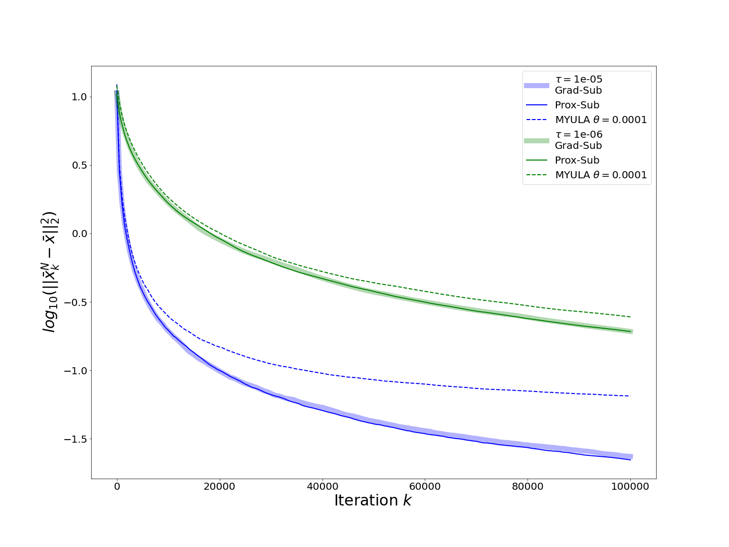
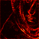
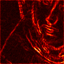
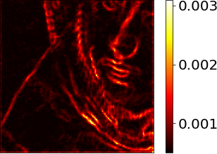
\newaliascnt

definitiontheorem \aliascntresetthedefinition \newaliascntcorollarytheorem \aliascntresetthecorollary \newaliascntpropositiontheorem \aliascntresettheproposition \newaliascntextheorem \aliascntresettheex \newaliascntlemmatheorem \aliascntresetthelemma \newaliascntdefproptheorem \aliascntresetthedefprop \newaliascntremarktheorem \aliascntresettheremark \newaliascntasstheorem \aliascntresettheass

Subgradient Langevin Methods for Sampling from Non-smooth Potentials

Andreas Habring    Martin Holler Institute of Mathematics and Scientific Computing, University of Graz. AH: andreas.habring@uni-graz.at, MH: martin.holler@uni-graz.at, https://imsc.uni-graz.at/hollerm.    Thomas Pock Institute of Computer Graphics and Vision, Graz University of Technology, Austria, pock@icg.tugraz.at.
Abstract

This paper is concerned with sampling from probability distributions π𝜋\pi on dsuperscript𝑑\mathbb{R}^{d} admitting a density of the form π(x)eU(x)proportional-to𝜋𝑥superscript𝑒𝑈𝑥\pi(x)\propto e^{-U(x)}, where U(x)=F(x)+G(Kx)𝑈𝑥𝐹𝑥𝐺𝐾𝑥U(x)=F(x)+G(Kx) with K𝐾K being a linear operator and G𝐺G being non-differentiable. Two different methods are proposed, both employing a subgradient step with respect to GK𝐺𝐾G\circ K, but, depending on the regularity of F𝐹F, either an explicit or an implicit gradient step with respect to F𝐹F. For both methods, non-asymptotic convergence proofs are provided, with improved convergence results for more regular F𝐹F. Further, numerical experiments are conducted for simple 2D examples, illustrating the convergence rates, and for examples of Bayesian imaging, showing the practical feasibility of the proposed methods for high dimensional data.

Key words. Markov chain Monte Carlo methods, Unadjasted Langevin algorithm, non-smooth sampling, Bayesian inference, Bayesian imaging, inverse problems.

MSC codes. 65C40 \cdot 65C05 \cdot 68U10 \cdot 65C60

1 Introduction

In this work we propose algorithms for sampling from a probability distribution π𝜋\pi on dsuperscript𝑑\mathbb{R}^{d} admitting a density - also denoted π𝜋\pi - of the form

π(x)=eU(x)eU(y)dy𝜋𝑥superscript𝑒𝑈𝑥superscript𝑒𝑈𝑦d𝑦\pi(x)=\frac{e^{-U(x)}}{\int e^{-U(y)\;\text{d}y}} (1.1)

with a potential U:d[0,):𝑈superscript𝑑0U:\mathbb{R}^{d}\rightarrow[0,\infty), U(x)=F(x)+G(Kx)𝑈𝑥𝐹𝑥𝐺𝐾𝑥U(x)=F(x)+G(Kx) where F:d[0,):𝐹superscript𝑑0F:\mathbb{R}^{d}\rightarrow[0,\infty), G:d[0,):𝐺superscriptsuperscript𝑑0G:\mathbb{R}^{d^{\prime}}\rightarrow[0,\infty) are both proper, convex, and lower semi-continuous (lsc), and K:dd:𝐾superscript𝑑superscriptsuperscript𝑑K:\mathbb{R}^{d}\rightarrow\mathbb{R}^{d^{\prime}} is a linear operator. Such exponential - or Gibbs - densities arise frequently in applications and are derived by a minimax entropy principle for image distributions in [41]. In particular, we are interested in the non-smooth setting that G𝐺G or both, F𝐹F and G𝐺G, are non-differentiable. More specifically, we assume the following regularity conditions.

Assumption \theass.

The functions F𝐹F and G𝐺G satisfy the following regularity assumptions:

  1. (1)

    F𝐹F is convex and

    1. (a)

      either Lipschitz continuous with constant LFsubscript𝐿𝐹L_{F}

    2. (b)

      or differentiable with Lipschitz continuous gradient with constant LFsubscript𝐿𝐹L_{\nabla F}.

  2. (2)

    G𝐺G is convex and Lipschitz continuous with constant LGsubscript𝐿𝐺L_{G}.

The task of sampling from such distributions frequently arises, e.g., in Bayesian inference in the field of mathematical imaging, see for instance [28, 13] for more background information, [39] and [40] for applications in magnetic resonance imaging and computed tomography, respectively, and [25] for error quantification based on sampling techniques. In this context, one is interested in inferring an unknown high-dimensional random variable Xd𝑋superscript𝑑X\in\mathbb{R}^{d} based on observing a random variable Yp(y|x)similar-to𝑌pconditional𝑦𝑥Y\sim\operatorname{p}(y|x). The distribution p(y|x)pconditional𝑦𝑥\operatorname{p}(y|x) and the so-called prior distribution p(x)p𝑥\operatorname{p}(x) are subject to modeling decisions and assumed to be known for our purposes. Using Bayes’ Theorem, the logarithm of the posterior distribution of X|Y=yconditional𝑋𝑌𝑦X|Y=y is easily seen to be

logp(x|y)=pconditional𝑥𝑦absent\displaystyle\log\operatorname{p}(x|y)= logp(y|x)+logp(x)logp(y).pconditional𝑦𝑥p𝑥p𝑦\displaystyle\log\operatorname{p}(y|x)+\log\operatorname{p}(x)-\log\operatorname{p}(y). (1.2)

Given an observation of Y𝑌Y, sampling from the posterior then allows not only to estimate X𝑋X by computing, e.g., its empirical expected value, but also to gauge the uncertainty of its estimate [25]. The function xlogp(y|x)+logp(x)logp(y)maps-to𝑥pconditional𝑦𝑥p𝑥p𝑦x\mapsto\log\operatorname{p}(y|x)+\log\operatorname{p}(x)-\log\operatorname{p}(y) here corresponds to F(x)G(Kx)𝐹𝑥𝐺𝐾𝑥-F(x)-G(Kx) in our general model. The specific structure of composing a non-differentiable functional G𝐺G with a linear operator K𝐾K allows for using a wide range of models for the log-prior such as logp(x)Kx1similar-top𝑥subscriptnorm𝐾𝑥1-\log\operatorname{p}(x)\sim\|Kx\|_{1} where K𝐾K can be, e.g., any transform promoting sparsity in a certain basis or frame, or a finite differences operator to obtain the famous Rudin-Osher-Fatemi TVL2TVsuperscript𝐿2\operatorname*{TV}-L^{2} model [32] or higher-order variants [3] from inverse problems and imaging111To be precise, p(x)exp(Kx1)proportional-top𝑥subscriptnorm𝐾𝑥1\operatorname{p}(x)\propto\exp(-\|Kx\|_{1}) frequently does not induce a well-defined probability distribution as p(x)dx=p𝑥d𝑥\int\operatorname{p}(x)\;\text{d}x=\infty if K𝐾K admits a non-trivial kernel. However, in conjunction with a suitable likelihood function, e.g., logp(y|x)=F(x)=xy22pconditional𝑦𝑥𝐹𝑥subscriptsuperscriptnorm𝑥𝑦22-\log\operatorname{p}(y|x)=F(x)=\|x-y\|^{2}_{2} for Gaussian denoising, the posterior distribution p(x|y)exp(F(x)Kx1)proportional-topconditional𝑥𝑦𝐹𝑥subscriptnorm𝐾𝑥1\operatorname{p}(x|y)\propto\exp(-F(x)-\|Kx\|_{1}) is, in fact, well defined..

In this work, we propose two different methods for sampling from π𝜋\pi. Both employ a subgradient step with respect to GK𝐺𝐾G\circ K, but depending on the regularity of F𝐹F, either an explicit or an implicit gradient step with respect to F𝐹F. We provide proofs of convergence for all methods, with improved results under stronger regularity assumptions on F𝐹F.

Typically, sampling from (1.1) is performed using Markov chain Monte Carlo methods. The strategy is to generate a Markov Chain (Xk)ksubscriptsubscript𝑋𝑘𝑘(X_{k})_{k} for which it is shown that the distribution of Xksubscript𝑋𝑘X_{k} approximates π𝜋\pi as k𝑘k\rightarrow\infty. A popular class of such methods are discretizations of the over-damped Langevin diffusion [31, 26]

dYt=U(Yt)dt+2dBtdsubscript𝑌𝑡𝑈subscript𝑌𝑡d𝑡2dsubscript𝐵𝑡\text{d}Y_{t}=-\nabla U(Y_{t})\;\text{d}t+\sqrt{2}\;\text{d}B_{t} (1.3)

with Btsubscript𝐵𝑡B_{t} denoting Brownian motion. Interestingly, as U=log(π)𝑈𝜋U=-\log(\pi) occurs solely in differentiated form in (1.3), such methods rely on knowledge of π(x)𝜋𝑥\pi(x) only up to a scalar multiple, that is, knowledge of the normalization constant eU(y)dysuperscript𝑒𝑈𝑦d𝑦\int e^{-U(y)}\;\text{d}y is not necessary. Indeed, under sufficient regularity conditions on U𝑈U, respectively U𝑈\nabla U, eq. 1.3 admits π𝜋\pi as a stationary distribution and the distribution of Ytsubscript𝑌𝑡Y_{t} converges to π𝜋\pi in total variation norm [30, Theorem 2.1] or in Wasserstein distance [2]. A discrete time Markov chain (MC) approximating (1.3) is obtained, e.g., via the Euler-Maruyama discretization, referred to as the Unadjusted Langevin Algorithm (ULA)

Xk+1=Xkγk+1U(Xk)+2γk+1Bk+1subscript𝑋𝑘1subscript𝑋𝑘subscript𝛾𝑘1𝑈subscript𝑋𝑘2subscript𝛾𝑘1subscript𝐵𝑘1X_{k+1}=X_{k}-\gamma_{k+1}\nabla U(X_{k})+\sqrt{2\gamma_{k+1}}\;B_{k+1} (1.4)

where γk>0subscript𝛾𝑘0\gamma_{k}>0 is the step size and (Bk)ksubscriptsubscript𝐵𝑘𝑘(B_{k})_{k} an i.i.d. sequence of d𝑑d-dimensional standard Gaussian random variables. For γk=γsubscript𝛾𝑘𝛾\gamma_{k}=\gamma for all k𝑘k, this MC admits a stationary distribution πγsubscript𝜋𝛾\pi_{\gamma} which is, in general, not equal to π𝜋\pi, but approximates π𝜋\pi in the sense that πγπsubscript𝜋𝛾𝜋\pi_{\gamma}\rightarrow\pi as γ0𝛾0\gamma\rightarrow 0 [10]. For γk0subscript𝛾𝑘0\gamma_{k}\rightarrow 0 with kγk=subscript𝑘subscript𝛾𝑘\sum_{k}\gamma_{k}=\infty, however, a direct approximation of π𝜋\pi without any bias is feasible [19]. Moreover, non-asymptotic convergence bounds have been shown in the total variation norm [12, 9] as well as in Wasserstein distance [11].

2 Related Works

The above mentioned works rely on differentiability of the potential U𝑈U, which is undesirable as many relevant applications naturally lead to non-differentiable potentials, e.g., regression with L1superscript𝐿1L^{1} loss or Lasso prior, or non-smooth regularization functionals in Bayesian imaging or inverse problems. Remedies for this issue have been proposed in the literature. For instance, in [13, 28] the authors propose to replace non-differentiable parts of the potential with its Moreau envelope leading to a continuously differentiable approximation of the potential as the Moreau envelope hλsuperscript𝜆h^{\lambda} with parameter λ>0𝜆0\lambda>0 of a (possibly non-differentiable) functional hh admits the Lipschitz continuous gradient hλ(x)=λ1(xproxλh(x))superscript𝜆𝑥superscript𝜆1𝑥subscriptprox𝜆𝑥\nabla h^{\lambda}(x)=\lambda^{-1}(x-{\operatorname*{prox}}_{\lambda h}(x)). This effectively leads to a proximal step with respect to non-differentiable parts of the potential U𝑈U. In [13] it is shown that the obtained smooth approximation of the target density can be made arbitrarily accurate in total variation (TV) by decreasing the Moreau-Yoshida parameter. The resulting method is coined MYULA (Moreau Yoshida Unadjusted Langevin Algorithm). In the method from [28], referred to as P-MALA (Proximal Metropolis Adjusted Langevin Algorithm), on the other hand, the discrepancy between the approximation and the true target density is accounted for by introducing a Metropolis-Hastings correction within the method. In [5], P-MALA is used for Bayesian model selection using a nested sampling procedure. In view potentials U𝑈U of the form U(x)=F(x)+G(Kx)𝑈𝑥𝐹𝑥𝐺𝐾𝑥U(x)=F(x)+G(Kx), a disadvantage of MYULA and P-MALA is that the proximal mapping of GK𝐺𝐾G\circ K will in general be accessible only via an iterative algorithm, rendering these approaches computationally expensive. In [4] the approach of [13] is investigated for the particular case of GK𝐺𝐾G\circ K being an indicator function on a compact, convex set. In [23] the authors extend the P-MALA approach to the case of non-convex potentials. It is shown that the smooth approximation of the density can be made arbitrarily accurate in TV. The authors also prove that the resulting continuous time Langevin diffusion admits a unique solution and a stationary distribution. Despite the weakened assumptions, convergence of the discretization of the Langevin diffusion is shown in expectation.

In [20], similarly to MYULA, the authors consider smoothing the target density. This time, however, the smoothing is achieved by convolving the non-smooth part with a Gaussian kernel. The gradient of the smoothed potential can be computed using Tweedie’s formula which leads to a Plug and Play approach [20].

In [10] the authors propose a subgradient as well as a proximal gradient method for direct sampling from non-smooth potentials without prior smoothing. While the former would allow for sampling from (1.1) in principle, it yields only suboptimal convergence behavior whenever F𝐹F is differentiable. Moreover, the subgradient method relies on Lipschitz continuity of F𝐹F, which prevents its applications, for example, to models with L2superscript𝐿2L^{2} loss. The proximal gradient method from [10], on the other hand, guarantees better convergence behavior, but again suffers from the fact that the proximal mapping of GK𝐺𝐾G\circ K is, in general, not explicit. Another approach has been proposed in [14] where the authors show that convergence can be maintained despite computing the proximal map only approximately, thus allowing also for its iterative computation within the algorithm. In [1] the authors propose a method that employs only the proximal mappings of F𝐹F and G𝐺G, but relies on invertibility of K𝐾K, which is not given in many cases of interest, such as K𝐾K being a finite differences operator.

In [22, 8, 21] the authors consider the regularized density π~(x,y)exp(U(x)μxy2)proportional-to~𝜋𝑥𝑦𝑈𝑥𝜇superscriptnorm𝑥𝑦2\tilde{\pi}(x,y)\propto\exp(-U(x)-\mu\|x-y\|^{2}) from which they sample using a Gibbs algorithm, where they sample alternatingly once using a so-called restricted Gaussian oracle to draw samples from π~(x|y)~𝜋conditional𝑥𝑦\tilde{\pi}(x|y) and once from the simple Gaussian π~(y|x)~𝜋conditional𝑦𝑥\tilde{\pi}(y|x). Note that the marginal density π~(x)=π~(x,y)dy=π(x)~𝜋𝑥~𝜋𝑥𝑦d𝑦𝜋𝑥\tilde{\pi}(x)=\int\tilde{\pi}(x,y)\;\text{d}y=\pi(x) is equal to the target density. The restricted Gaussian oracle is implemented via a rejection sampling subroutine. In [22] the authors focus on non-differentiable but Lipschitz continuous potentials. In [21] these techniques are applied to potentials of the form U(x)=F(x)+G(x)𝑈𝑥𝐹𝑥𝐺𝑥U(x)=F(x)+G(x) with F𝐹F strongly convex and a Lipschitz continuous gradient F𝐹\nabla F but possibly non-smooth G𝐺G. In [8] the convergence results from [21] are extended to the case of potentials which are not strongly convex. A downside of these alternating sampling methods is the requirement of subroutines for the computation of the restricted Gaussian oracle which might render iterations more expensive than in the case of Langevin based algorithms.

In the [37] the authors propose a splitting technique resembling an Alternating Direction Method of Multipliers (ADMM) type approach. That is, by introducing an auxiliary variable z𝑧z, a density of the form π(x)exp(F(x)G(x))proportional-to𝜋𝑥𝐹𝑥𝐺𝑥\pi(x)\propto\exp(-F(x)-G(x)) is approximated by π~(x,y)=exp(F(x)G(y)ϕ(x,y))~𝜋𝑥𝑦𝐹𝑥𝐺𝑦italic-ϕ𝑥𝑦\tilde{\pi}(x,y)=\exp(-F(x)-G(y)-\phi(x,y)) where ϕitalic-ϕ\phi is a functional penalizing large deviations between x𝑥x and y𝑦y. The authors show that for appropriate ϕitalic-ϕ\phi the marginal density of π~~𝜋\tilde{\pi} with respect to x𝑥x approximates π𝜋\pi in TV distance. Thus samples from π𝜋\pi can be approximated by sampling from π~~𝜋\tilde{\pi} using Gibbs sampling, that is again, sampling from π~(x|y)~𝜋conditional𝑥𝑦\tilde{\pi}(x|y) and π~(y|x)~𝜋conditional𝑦𝑥\tilde{\pi}(y|x) in an alternating fashion. Such an approach, dividing the sampling problem into two easier sub-problems, could be interesting for the task considered in the present work in particular when also F𝐹F is non-smooth. A similar approach is taken in [38], where for potentials of the form π(x)exp(U(Kx))proportional-to𝜋𝑥𝑈𝐾𝑥\pi(x)\propto\exp(-U(Kx)) with a linear operator K𝐾K the auxiliary density is defined as π~(x,y)=exp(U(x)Kxy22/(2ρ2))~𝜋𝑥𝑦𝑈𝑥subscriptsuperscriptnorm𝐾𝑥𝑦222superscript𝜌2\tilde{\pi}(x,y)=\exp(-U(x)-\|Kx-y\|^{2}_{2}/(2\rho^{2})) such that a decoupling of operator and functional is achieved. Also in this work sampling is done by employing a Gibbs sampling scheme. A downside of these approaches is, similar to the above approaches based on restricted Gaussian oracles, that the Gibbs sampling potentially requires a subsampling scheme in each iteration. As such a subroutine, in [37] the authors propose to use MYULA [13] or P-MALA [28], whereas in [38] rejection sampling is utilized.

In the present work we propose two methods for sampling from the potential π(x)𝜋𝑥\pi(x) in (1.1), a Proximal-subgradient (Prox-sub) as well as a Gradient-subgradient (Grad-sub) method. The methods employ only the subgradient of G𝐺G, evaluation of K𝐾K and Ksuperscript𝐾K^{*} and the gradient, respectively proximal mapping, of F𝐹F. Inspired by the results and techniques introduced in [10], our main algorithm combines the benefits of different methods of [10] in the sense that it is applicable in the non-smooth case while simultaneously ensuring superior convergence in the smooth case. For a comparison of the complexities of the proposed methods to the state of the art we refer to Table 2.1, where we show the computational complexity to reach a given accuracy of the sample distribution to the target in the Wasserstein-2 distance, the Kullback-Leibler divergence (KL) and the TV. While in some cases the proposed methods exhibit a greater computational effort, its main advantage is the broad applicability to settings where for other algorithms a subroutine for the computation of proximal mappings is necessary. In summary the contributions of the present work are the following:

  • We propose two Langevin algorithms for sampling from potentials of the form U(x)=F(x)+G(Kx)𝑈𝑥𝐹𝑥𝐺𝐾𝑥U(x)=F(x)+G(Kx), with G𝐺G non-differentiable and the proximal mapping of GK𝐺𝐾G\circ K not being explicit. To the best of our knowledge, this is the first Langevin-type sampling algorithm (without inner iterations) that is applicable to a potential of the above form, with F𝐹F not necessarily being Lipschitz continuous. In particular, it is the first algorithm that allows guaranteed sampling from models like the the TVL2TVsuperscript𝐿2\operatorname*{TV}-L^{2} model [32] or generalizations to inverse problems with L2superscript𝐿2L^{2} data discrepancy [3].

  • We provide non-asymptotic convergence results for the proposed algorithms for the case that F𝐹F is non-differentiable as well as improved results for the case that F𝐹F satisfies stronger regularity assumptions. The results are non-asymptotic in the sense that a desired accuracy is reached after a finite and explicitly known number of iterations.

  • We provide comprehensive numerical results confirming all proven convergence rates in a 2D setting. The practical feasibility of the methods for high-dimensional data is further demonstrated via examples from Bayesian imaging.

Assumptions on F𝐹F
Lipschitz continuous Lipschitz gradient Lipschitz gradient, strongly convex
TV KL TV KL TV KL W22subscriptsuperscript𝑊22W^{2}_{2}
Prox-sub dϵ6𝑑superscriptitalic-ϵ6d\epsilon^{-6} dϵ3𝑑superscriptitalic-ϵ3d\epsilon^{-3} dϵ4𝑑superscriptitalic-ϵ4d\epsilon^{-4} dϵ2𝑑superscriptitalic-ϵ2d\epsilon^{-2} dϵ4𝑑superscriptitalic-ϵ4d\epsilon^{-4} dϵ2𝑑superscriptitalic-ϵ2d\epsilon^{-2} dlog(ϵ1)ϵ𝑑superscriptitalic-ϵ1italic-ϵd\frac{\log(\epsilon^{-1})}{\epsilon}
Grad-sub - - dϵ4𝑑superscriptitalic-ϵ4d\epsilon^{-4} dϵ2𝑑superscriptitalic-ϵ2d\epsilon^{-2} dϵ4𝑑superscriptitalic-ϵ4d\epsilon^{-4} dϵ2𝑑superscriptitalic-ϵ2d\epsilon^{-2} dlog(ϵ1)ϵ𝑑superscriptitalic-ϵ1italic-ϵd\frac{\log(\epsilon^{-1})}{\epsilon}
MYULA [13] d5log2(ϵ1)ϵ2superscript𝑑5superscript2superscriptitalic-ϵ1superscriptitalic-ϵ2d^{5}\frac{\log^{2}(\epsilon^{-1})}{\epsilon^{2}} - d5log2(ϵ1)ϵ2superscript𝑑5superscript2superscriptitalic-ϵ1superscriptitalic-ϵ2d^{5}\frac{\log^{2}(\epsilon^{-1})}{\epsilon^{2}} - dlog(d)log2(ϵ1)ϵ2𝑑𝑑superscript2superscriptitalic-ϵ1superscriptitalic-ϵ2d\log(d)\frac{\log^{2}(\epsilon^{-1})}{\epsilon^{2}} - -
SSGLD [10] ϵ4superscriptitalic-ϵ4\epsilon^{-4} ϵ2superscriptitalic-ϵ2\epsilon^{-2} - - - - -
SPGLD [10] - - dϵ4𝑑superscriptitalic-ϵ4d\epsilon^{-4} dϵ2𝑑superscriptitalic-ϵ2d\epsilon^{-2} dϵ4𝑑superscriptitalic-ϵ4d\epsilon^{-4} dϵ2𝑑superscriptitalic-ϵ2d\epsilon^{-2} dϵ2𝑑superscriptitalic-ϵ2d\epsilon^{-2}
[22] log(d1/2ϵ1)ϵsuperscript𝑑12superscriptitalic-ϵ1italic-ϵ\frac{\log(d^{1/2}\epsilon^{-1})}{\epsilon} - - - - - -
Table 2.1: Computational complexities of the proposed methods and existing methods in terms of the accuracy ϵitalic-ϵ\epsilon and the dimension d𝑑d. The entries depict the order of the necessary number of iterations to reach accuracy ϵitalic-ϵ\epsilon to the target density in a specific metric. Gray entries indicate cases where it is necessary to iteratively compute the proximal mapping of GK𝐺𝐾G\circ K, or even F+GK𝐹𝐺𝐾F+G\circ K, which is not explicit in general for non-trivial K𝐾K. MYULA is initialized with the Dirac distribution at an arbitrary point. The method from [22] is initialized at a minimizer of the potential U𝑈U regularized by a quadratic term. For the remaining methods we assume initialization using a warm start such that the Wasserstein-2 distance to the target density of the initial distribution is bounded by a constant. In all cases G𝐺G is only assumed to be convex and Lipschitz continous. Here, SSGLD stands for Stochastic SubGradient Langevin Dynamics and SPGLD stands for Stochastic Proximal Gradient Langevin Dynamics

A limitation of our work is that, so far, we were were not able to establish ergodicity and existence and uniqueness of a stationary measure for the transition kernel corresponding to one iteration of our algorithm. This has the disadvantage that, for sampling, several parallel Markov chains are required instead of a singel chain from which successive samples can be used. Existing literature typically relies on differentiability of the potential U𝑈U in order to show that a stationary measure for the transition kernel exists and that the corresponding Markov chain is geometrically ergodic [12, 10, 30, 28, 13]. However, due to the non-differentiability of the considered potentials and the fact that we do not consider a smoothed approximation of the potential U𝑈U, an application of these results is not feasible in our setting.

Outline of the paper

The remainder of the paper is organized as follows. After introducing the notation and listing some essential preliminary results in Section 3, we present the proposed algorithms in Sections 4 and 6. For each method we provide corresponding non-asymptotic convergence results in the respective section. Numerical experiments and a brief conclusion are further provided in Sections 7 and 8, respectively.

3 Notation and Preliminaries

Slightly abusing notation, we write \|\;\cdot\;\| for both the 222-norm on dsuperscript𝑑\mathbb{R}^{d} and the norm of a linear operator. A proper function f:d(,]:𝑓superscript𝑑f:\mathbb{R}^{d}\rightarrow(-\infty,\infty] is called m𝑚m-strongly convex if for any x,yd𝑥𝑦superscript𝑑x,y\in\mathbb{R}^{d} and λ(0,1)𝜆01\lambda\in(0,1)

f(λx+(1λ)y)λf(x)+(1λ)f(y)mλ(1λ)2xy2.𝑓𝜆𝑥1𝜆𝑦𝜆𝑓𝑥1𝜆𝑓𝑦𝑚𝜆1𝜆2superscriptnorm𝑥𝑦2f(\lambda x+(1-\lambda)y)\leq\lambda f(x)+(1-\lambda)f(y)-m\frac{\lambda(1-\lambda)}{2}\|x-y\|^{2}.

For a convex function f:d(,]:𝑓superscript𝑑f:\mathbb{R}^{d}\rightarrow(-\infty,\infty] we define the subdifferential as the (possibly empty) set

f(x)={yd|hd:f(x)+y,x+hf(x+h)},𝑓𝑥conditional-set𝑦superscript𝑑:for-allsuperscript𝑑𝑓𝑥𝑦𝑥𝑓𝑥\partial f(x)=\left\{y\in\mathbb{R}^{d}\;\middle|\;\forall h\in\mathbb{R}^{d}:\;f(x)+\langle y,x+h\rangle\leq f(x+h)\right\},

where ,\langle\cdot,\cdot\rangle denotes that standard inner product between vectors in dsuperscript𝑑\mathbb{R}^{d}. For proper, convex, and lsc f𝑓f, f(x)𝑓𝑥\partial f(x)\neq\emptyset for any x(dom(f))𝑥superscriptdom𝑓x\in(\operatorname*{dom}(f))^{\circ}, the interior of dom(f)dom𝑓\operatorname*{dom}(f), where dom(f){xd|f(x)<}dom𝑓conditional-set𝑥superscript𝑑𝑓𝑥\operatorname*{dom}(f)\coloneqq\left\{x\in\mathbb{R}^{d}\;\middle|\;f(x)<\infty\right\}. We further define the proximal mapping of f𝑓f as

proxf(x)=argminzdf(z)+12xz2.subscriptprox𝑓𝑥subscriptargmin𝑧superscript𝑑𝑓𝑧12superscriptnorm𝑥𝑧2{\operatorname*{prox}}_{f}(x)=\operatorname*{argmin}_{z\in\mathbb{R}^{d}}f(z)+\frac{1}{2}\|x-z\|^{2}. (3.1)

If f𝑓f is proper, convex, and lsc, proxf(x)subscriptprox𝑓𝑥{\operatorname*{prox}}_{f}(x) is well-defined and single-valued for any x𝑥x, that is, the minimizer in (3.1) exists and is unique. We denote the Borel σ𝜎\sigma-algebra on dsuperscript𝑑\mathbb{R}^{d} as (d)superscript𝑑\mathcal{B}(\mathbb{R}^{d}) and the set of probability measures on the measurable space (d,(d))superscript𝑑superscript𝑑(\mathbb{R}^{d},\mathcal{B}(\mathbb{R}^{d})) as 𝒫(d)𝒫superscript𝑑\mathcal{P}(\mathbb{R}^{d}). A Markov transition kernel is a function S:d×(d)[0,1]:𝑆superscript𝑑superscript𝑑01S:\mathbb{R}^{d}\times\mathcal{B}(\mathbb{R}^{d})\rightarrow[0,1] such that S(,A)𝑆𝐴S(\;\cdot\;,A) is measurable for any A𝐴A and S(x,)𝑆𝑥S(x,\;\cdot\;) is a probability measure for any x𝑥x. We denote the application of the kernel S𝑆S to a probability measure μ𝒫(d)𝜇𝒫superscript𝑑\mu\in\mathcal{P}(\mathbb{R}^{d}) as μS𝜇𝑆\mu S defined as

μS(A)=S(x,A)dμ(x)𝜇𝑆𝐴𝑆𝑥𝐴d𝜇𝑥\mu S(A)=\int S(x,A)\;\text{d}\mu(x)

which is again a probability measure. If there exists a density g𝑔g such that S(x,A)=Ag(x,y)dy𝑆𝑥𝐴subscript𝐴𝑔𝑥𝑦d𝑦S(x,A)=\int_{A}g(x,y)\;\text{d}y, Fubini’s theorem implies that yg(x,y)dμ(x)maps-to𝑦𝑔𝑥𝑦d𝜇𝑥y\mapsto\int g(x,y)\;\text{d}\mu(x) is a density of μS𝜇𝑆\mu S and, therefore, we can compute the integral of a function f𝑓f with respect to μS𝜇𝑆\mu S as

f(y)dμS(y)=f(y)g(x,y)dμ(x)dy.𝑓𝑦d𝜇𝑆𝑦𝑓𝑦𝑔𝑥𝑦d𝜇𝑥d𝑦\int f(y)\;\text{d}\mu S(y)=\int\int f(y)g(x,y)\;\text{d}\mu(x)\text{d}y. (3.2)

Let 𝒫2(d)subscript𝒫2superscript𝑑\mathcal{P}_{2}(\mathbb{R}^{d}) denote the set of all probability measures with finite second moment, that is, all μ𝒫(d)𝜇𝒫superscript𝑑\mu\in\mathcal{P}(\mathbb{R}^{d}) such that x2dμ(x)<superscriptnorm𝑥2d𝜇𝑥\int\|x\|^{2}\;\text{d}\mu(x)<\infty. We write μνmuch-less-than𝜇𝜈\mu\ll\nu if μ𝜇\mu is absolutely continuous with respect to ν𝜈\nu and in this case the Radon-Nikodým derivative of μ𝜇\mu with respect to ν𝜈\nu is denoted as dμdνd𝜇d𝜈\frac{\text{d}\mu}{\text{d}\nu}. By (Bk)ksubscriptsubscript𝐵𝑘𝑘(B_{k})_{k} we alweays denote an i.i.d. sequence of d𝑑d-dimensional standard Gaussian random variables. The Kullback-Leibler (KL) divergence between two measures μ,ν𝒫(d)𝜇𝜈𝒫superscript𝑑\mu,\nu\in\mathcal{P}(\mathbb{R}^{d}) is defined as

KL(μ|ν)={dμdν(x)log(dμdν(x))dν(x)if μνotherwise.KLconditional𝜇𝜈casesd𝜇d𝜈𝑥d𝜇d𝜈𝑥d𝜈𝑥much-less-thanif 𝜇𝜈otherwise.\operatorname*{KL}(\mu|\nu)=\begin{cases}\int\frac{\text{d}\mu}{\text{d}\nu}(x)\log(\frac{\text{d}\mu}{\text{d}\nu}(x))\;\text{d}\nu(x)\quad&\text{if }\mu\ll\nu\\ \infty\quad&\text{otherwise.}\end{cases} (3.3)

A coupling of μ𝜇\mu and ν𝜈\nu is a probability measure ζ𝜁\zeta on d×dsuperscript𝑑superscript𝑑\mathbb{R}^{d}\times\mathbb{R}^{d} with marginal distributions μ𝜇\mu and ν𝜈\nu, that is, for any A(d)𝐴superscript𝑑A\in\mathcal{B}(\mathbb{R}^{d}), ζ(A×d)=μ(A)𝜁𝐴superscript𝑑𝜇𝐴\zeta(A\times\mathbb{R}^{d})=\mu(A) and ζ(d×A)=ν(A)𝜁superscript𝑑𝐴𝜈𝐴\zeta(\mathbb{R}^{d}\times A)=\nu(A). We denote the set of all couplings of μ𝜇\mu and ν𝜈\nu as Π(μ,ν)Π𝜇𝜈\Pi(\mu,\nu). In a slight abuse of terminology, we will also refer to a couple of random variables (X,Y)𝑋𝑌(X,Y) as a coupling of μ𝜇\mu and ν𝜈\nu if there exists ζΠ(μ,ν)𝜁Π𝜇𝜈\zeta\in\Pi(\mu,\nu) such that (X,Y)𝑋𝑌(X,Y) is distributed according to ζ𝜁\zeta. The (Kantorovich) Wasserstein 2-distance between two measures μ,ν𝒫2(d)𝜇𝜈subscript𝒫2superscript𝑑\mu,\nu\in\mathcal{P}_{2}(\mathbb{R}^{d}) is defined as

W2(μ,ν)=(infζΠ(μ,ν)xy2dζ(x,y))1/2.subscript𝑊2𝜇𝜈superscriptsubscriptinfimum𝜁Π𝜇𝜈superscriptnorm𝑥𝑦2d𝜁𝑥𝑦12W_{2}(\mu,\nu)=\left(\inf\limits_{\zeta\in\Pi(\mu,\nu)}\int\|x-y\|^{2}\;\text{d}\zeta(x,y)\right)^{1/2}. (3.4)

By [36] the infimum in the definition of the Wasserstein 2-distance is, in fact, attained, i.e., there exists a coupling ζsuperscript𝜁\zeta^{*} such that W22(μ,ν)=xy2dζ(x,y)=E[XY2]subscriptsuperscript𝑊22𝜇𝜈superscriptnorm𝑥𝑦2dsuperscript𝜁𝑥𝑦Esuperscriptnorm𝑋𝑌2W^{2}_{2}(\mu,\nu)=\int\|x-y\|^{2}\;\text{d}\zeta^{*}(x,y)=\operatorname{E}[\|X-Y\|^{2}] for (X,Y)ζsimilar-to𝑋𝑌superscript𝜁(X,Y)\sim\zeta^{*}. We will refer to ζsuperscript𝜁\zeta^{*}, respectively (X,Y)𝑋𝑌(X,Y), as an optimal coupling for μ,ν𝜇𝜈\mu,\nu.

For a potential V:d[0,):𝑉superscript𝑑0V:\mathbb{R}^{d}\rightarrow[0,\infty) we define the potential energy and the Boltzman H-functional V,:𝒫2(d)[0,]:subscript𝑉subscript𝒫2superscript𝑑0\mathcal{E}_{V},\mathcal{H}:\mathcal{P}_{2}(\mathbb{R}^{d})\rightarrow[0,\infty] as

V(μ)subscript𝑉𝜇\displaystyle\mathcal{E}_{V}(\mu) =V(x)dμ(x),and(μ)absent𝑉𝑥d𝜇𝑥and𝜇\displaystyle=\int V(x)\;\text{d}\mu(x),\quad\text{and}\quad\mathcal{H}(\mu) =KL(μ|Leb),absentKLconditional𝜇Leb\displaystyle=\operatorname*{KL}(\mu|\operatorname*{Leb}), (3.5)

respectively, where Leb denotes the Lebesgue measure. Further, for the given potential U𝑈U from (1.1) we define the free energy functional =+U=+F+GKsubscript𝑈subscript𝐹subscript𝐺𝐾\mathcal{F}=\mathcal{H}+\mathcal{E}_{U}=\mathcal{H}+\mathcal{E}_{F}+\mathcal{E}_{G\circ K}. The relevance of the free energy functional is evident from the following result.

Lemma \thelemma.

It holds that

  • π𝒫2(d)𝜋subscript𝒫2superscript𝑑\pi\in\mathcal{P}_{2}(\mathbb{R}^{d}), U(π)<subscript𝑈𝜋\mathcal{E}_{U}(\pi)<\infty, and (π)<𝜋\mathcal{H}(\pi)<\infty.

  • For μ𝒫2(d)𝜇subscript𝒫2superscript𝑑\mu\in\mathcal{P}_{2}(\mathbb{R}^{d}) with U(μ)<subscript𝑈𝜇\mathcal{E}_{U}(\mu)<\infty it holds that (μ)(π)=KL(μ|π)𝜇𝜋KLconditional𝜇𝜋\mathcal{F}(\mu)-\mathcal{F}(\pi)=\operatorname*{KL}(\mu|\pi).

For a proof see [10, Lemma 1]. This result implies that (μ)(π)0𝜇𝜋0\mathcal{F}(\mu)-\mathcal{F}(\pi)\geq 0 with equality if and only if μ=π𝜇𝜋\mu=\pi. It further allows us to formulate the task of sampling as a minimization problem. Namely, if (Xk)ksubscriptsubscript𝑋𝑘𝑘(X_{k})_{k} denotes the MC used to approximate the distribution π𝜋\pi, and μksubscript𝜇𝑘\mu_{k} the distribution of Xksubscript𝑋𝑘X_{k}, then convergence of the MC is ensured if μksubscript𝜇𝑘\mu_{k} minimizes μ(μ)(π)maps-to𝜇𝜇𝜋\mu\mapsto\mathcal{F}(\mu)-\mathcal{F}(\pi) in the limit.

4 Proximal-subgradient Langevin Sampling

In this section we investigate the first of the proposed sampling methods, namely the Proximal-subgradient Langevin algorithm (Prox-sub). The main results of this section will be Theorems 4.2 and 4 where we show convergence of the running mean of the sample distributions in KL to the target density. The algorithm is depicted in Algorithm 4.1. One iteration of the method consists of a subgradient step with respect to GK𝐺𝐾G\circ K and a proximal step with respect to F𝐹F followed by adding the Gaussian random variable Bk+1subscript𝐵𝑘1B_{k+1}. In particular, the method is feasible in the case that both F𝐹F and G𝐺G are non-differentiable. At this point it might seem unusual to apply different step sizes τksubscript𝜏𝑘\tau_{k} and τk+1subscript𝜏𝑘1\tau_{k+1} within a single iteration of Algorithm 4.1. In the way the algorithm is presented, the step size of proximal step with respect to F𝐹F in iteration k𝑘k is identical to the step size of the subgradient update for GK𝐺𝐾G\circ K in iteration k+1𝑘1k+1 which will turn out to be favorable within the proofs of convergence, see Section 4.

Algorithm 4.1 Proximal-subgradient Langevin Algorithm (Prox-sub)

Input: Initialization X0subscript𝑋0X_{0}, number of iterations K𝐾K, step sizes (τk)k=0Ksuperscriptsubscriptsubscript𝜏𝑘𝑘0𝐾(\tau_{k})_{k=0}^{K}, τk>0subscript𝜏𝑘0\tau_{k}>0.

1:for k=0,1,2,,K1𝑘012𝐾1k=0,1,2,\dots,K-1 do
2:     Pick Yk+1G(KXk)subscript𝑌𝑘1𝐺𝐾subscript𝑋𝑘Y_{k+1}\in\partial G(KX_{k})
3:     Xk+1=proxτk+1F(XkτkKYk+1)+2τk+1Bk+1subscript𝑋𝑘1subscriptproxsubscript𝜏𝑘1𝐹subscript𝑋𝑘subscript𝜏𝑘superscript𝐾subscript𝑌𝑘12subscript𝜏𝑘1subscript𝐵𝑘1X_{k+1}={\operatorname*{prox}}_{\tau_{k+1}F}(X_{k}-\tau_{k}K^{*}Y_{k+1})+\sqrt{2\tau_{k+1}}B_{k+1}
4:end for

Output: XKsubscript𝑋𝐾X_{K}.

Let μksubscript𝜇𝑘\mu_{k} denote the distribution of Xksubscript𝑋𝑘X_{k}. In accordance with the algorithm, we define the following Markov transition kernels

{SτG(x,A)=δxτKθ(Kx)(A)SτF(x,A)=δproxτF(x)(A)Tτ(x,A)=(4πτ)d/2Aexp(xz2/(4τ))dzcasessubscriptsuperscript𝑆𝐺𝜏𝑥𝐴subscript𝛿𝑥𝜏superscript𝐾𝜃𝐾𝑥𝐴otherwisesubscriptsuperscript𝑆𝐹𝜏𝑥𝐴subscript𝛿subscriptprox𝜏𝐹𝑥𝐴otherwisesubscript𝑇𝜏𝑥𝐴superscript4𝜋𝜏𝑑2subscript𝐴superscriptnorm𝑥𝑧24𝜏d𝑧otherwise\begin{cases}S^{G}_{\tau}(x,A)=\delta_{x-\tau K^{*}\theta(Kx)}(A)\\ S^{F}_{\tau}(x,A)=\delta_{{\operatorname*{prox}}_{\tau F}(x)}(A)\\ T_{\tau}(x,A)=(4\pi\tau)^{-d/2}\int\limits_{A}\exp\left(-\left\|x-z\right\|^{2}\middle/(4\tau)\right)\;\text{d}z\end{cases} (4.1)

where δx𝒫2(d)subscript𝛿𝑥subscript𝒫2superscript𝑑\delta_{x}\in\mathcal{P}_{2}(\mathbb{R}^{d}) denotes the Dirac measure concentrated in x𝑥x and θ:dd:𝜃superscript𝑑superscript𝑑\theta:\mathbb{R}^{d}\rightarrow\mathbb{R}^{d} is a measurable function such that for any zd𝑧superscriptsuperscript𝑑z\in\mathbb{R}^{d^{\prime}}, θ(z)G(z)𝜃𝑧𝐺𝑧\theta(z)\in\partial G(z). We introduce the notation Rτ~,τSτ~GSτFTτsubscript𝑅~𝜏𝜏subscriptsuperscript𝑆𝐺~𝜏subscriptsuperscript𝑆𝐹𝜏subscript𝑇𝜏R_{\tilde{\tau},\tau}\coloneqq S^{G}_{\tilde{\tau}}S^{F}_{\tau}T_{\tau} so that the iteration on the distributions (μk)ksubscriptsubscript𝜇𝑘𝑘(\mu_{k})_{k} induced by Algorithm 4.1 can be written as

μk+1=μkRτk,τk+1.subscript𝜇𝑘1subscript𝜇𝑘subscript𝑅subscript𝜏𝑘subscript𝜏𝑘1\mu_{k+1}=\mu_{k}R_{\tau_{k},\tau_{k+1}}. (4.2)

Note that Rτ~,τSτ~GSτFTτsubscript𝑅~𝜏𝜏subscriptsuperscript𝑆𝐺~𝜏subscriptsuperscript𝑆𝐹𝜏subscript𝑇𝜏R_{\tilde{\tau},\tau}\coloneqq S^{G}_{\tilde{\tau}}S^{F}_{\tau}T_{\tau} (and similar for other transition kernels) is purely symbolic notation that only makes sense in conjunction with the application to a probability measure μ𝜇\mu, were for the latter we use the order μRτ~,τ=((μSτ~G)SτF)Tτ𝜇subscript𝑅~𝜏𝜏𝜇subscriptsuperscript𝑆𝐺~𝜏subscriptsuperscript𝑆𝐹𝜏subscript𝑇𝜏\mu R_{\tilde{\tau},\tau}=((\mu S^{G}_{\tilde{\tau}})S^{F}_{\tau})T_{\tau}. As mentioned above, the existence and uniqueness of a stationary measure for the kernel Rτ~,τsubscript𝑅~𝜏𝜏R_{\tilde{\tau},\tau} is still an open question. Instead of proving ergodicity of the Markov chain generated by Rτ~,τsubscript𝑅~𝜏𝜏R_{\tilde{\tau},\tau}, thus, the strategy for proving convergence of the proposed algorithm is to directly bound the discrepancy between μksubscript𝜇𝑘\mu_{k} and π𝜋\pi in a suitable metric. To achieve this, we closely follow [10], that is, we will derive a bound for (μk)(π)=KL(μk|π)subscript𝜇𝑘𝜋KLconditionalsubscript𝜇𝑘𝜋\mathcal{F}(\mu_{k})-\mathcal{F}(\pi)=\operatorname*{KL}(\mu_{k}|\pi) along the iteration (4.2). In order to do so we will make use of the decomposition

(μRτ~,τ)(π)=F(μSτ~GSτFTτ)F(μSτ~GSτF)𝜇subscript𝑅~𝜏𝜏𝜋subscript𝐹𝜇subscriptsuperscript𝑆𝐺~𝜏subscriptsuperscript𝑆𝐹𝜏subscript𝑇𝜏subscript𝐹𝜇subscriptsuperscript𝑆𝐺~𝜏subscriptsuperscript𝑆𝐹𝜏\displaystyle\mathcal{F}(\mu R_{\tilde{\tau},\tau})-\mathcal{F}(\pi)=\mathcal{E}_{F}(\mu S^{G}_{\tilde{\tau}}S^{F}_{\tau}T_{\tau})-\mathcal{E}_{F}(\mu S^{G}_{\tilde{\tau}}S^{F}_{\tau}) (4.3)
+F(μSτ~GSτF)F(π)subscript𝐹𝜇subscriptsuperscript𝑆𝐺~𝜏subscriptsuperscript𝑆𝐹𝜏subscript𝐹𝜋\displaystyle+\mathcal{E}_{F}(\mu S^{G}_{\tilde{\tau}}S^{F}_{\tau})-\mathcal{E}_{F}(\pi)
+GK(μSτ~GSτFTτ)GK(π)subscript𝐺𝐾𝜇subscriptsuperscript𝑆𝐺~𝜏subscriptsuperscript𝑆𝐹𝜏subscript𝑇𝜏subscript𝐺𝐾𝜋\displaystyle+\mathcal{E}_{G\circ K}(\mu S^{G}_{\tilde{\tau}}S^{F}_{\tau}T_{\tau})-\mathcal{E}_{G\circ K}(\pi)
+(μSτ~GSτFTτ)(π)𝜇subscriptsuperscript𝑆𝐺~𝜏subscriptsuperscript𝑆𝐹𝜏subscript𝑇𝜏𝜋\displaystyle+\mathcal{H}(\mu S^{G}_{\tilde{\tau}}S^{F}_{\tau}T_{\tau})-\mathcal{H}(\pi)

for which we will derive estimates for each difference separately.

Lemma \thelemma.

Let μ𝒫2(d)𝜇subscript𝒫2superscript𝑑\mu\in\mathcal{P}_{2}(\mathbb{R}^{d}). If F𝐹F is LFsubscript𝐿𝐹L_{F}-Lipschitz continuous it holds true that

F(μTτ)F(μ)LF2dτsubscript𝐹𝜇subscript𝑇𝜏subscript𝐹𝜇subscript𝐿𝐹2𝑑𝜏\mathcal{E}_{F}(\mu T_{\tau})-\mathcal{E}_{F}(\mu)\leq L_{F}\sqrt{2d\tau}

and if F𝐹F is differentiable with LFsubscript𝐿𝐹L_{\nabla F}-Lipschitz gradient, then

F(μTτ)F(μ)τLFd.subscript𝐹𝜇subscript𝑇𝜏subscript𝐹𝜇𝜏subscript𝐿𝐹𝑑\mathcal{E}_{F}(\mu T_{\tau})-\mathcal{E}_{F}(\mu)\leq\tau L_{\nabla F}d.
Proof.

If F𝐹F is Lipschitz continuous a simple computation yields

F(μTγ)F(μ)=F(x)d(μTτ)(x)F(x)dμ(x)subscript𝐹𝜇subscript𝑇𝛾subscript𝐹𝜇𝐹𝑥d𝜇subscript𝑇𝜏𝑥𝐹𝑥d𝜇𝑥\displaystyle\mathcal{E}_{F}(\mu T_{\gamma})-\mathcal{E}_{F}(\mu)=\int F(x)\;\text{d}(\mu T_{\tau})(x)-\int F(x)\;\text{d}\mu(x) (4.4)
=(4πτ)d/2(F(x+y)F(x))ey24τdμ(x)dyabsentsuperscript4𝜋𝜏𝑑2𝐹𝑥𝑦𝐹𝑥superscript𝑒superscriptnorm𝑦24𝜏d𝜇𝑥d𝑦\displaystyle=(4\pi\tau)^{-d/2}\int\int(F(x+y)-F(x))e^{\frac{-\|y\|^{2}}{4\tau}}\;\text{d}\mu(x)\text{d}y
(4πτ)d/2LFyey24τdμ(x)dyabsentsuperscript4𝜋𝜏𝑑2subscript𝐿𝐹norm𝑦superscript𝑒superscriptnorm𝑦24𝜏d𝜇𝑥d𝑦\displaystyle\leq(4\pi\tau)^{-d/2}\int\int L_{F}\|y\|e^{\frac{-\|y\|^{2}}{4\tau}}\;\text{d}\mu(x)\text{d}y
((4πτ)d/2LF2y2ey24τdy)12=LFd2τ.absentsuperscriptsuperscript4𝜋𝜏𝑑2superscriptsubscript𝐿𝐹2superscriptnorm𝑦2superscript𝑒superscriptnorm𝑦24𝜏d𝑦12subscript𝐿𝐹𝑑2𝜏\displaystyle\leq\left((4\pi\tau)^{-d/2}\int L_{F}^{2}\|y\|^{2}e^{\frac{-\|y\|^{2}}{4\tau}}\;\text{d}y\right)^{\frac{1}{2}}=L_{F}\sqrt{d2\tau}.

If F𝐹F is differentiable with Lipschitz gradient the fundamental theorem of calculus leads to

F(y)F(x)F(x),yx𝐹𝑦𝐹𝑥𝐹𝑥𝑦𝑥\displaystyle F(y)-F(x)-\langle\nabla F(x),y-x\rangle =01F(x+t(yx))F(x),yxdtabsentsuperscriptsubscript01𝐹𝑥𝑡𝑦𝑥𝐹𝑥𝑦𝑥d𝑡\displaystyle=\int\limits_{0}^{1}\langle\nabla F(x+t(y-x))-\nabla F(x),y-x\rangle\;\text{d}t (4.5)
01LFtyx2dtLF2yx2.absentsuperscriptsubscript01subscript𝐿𝐹𝑡superscriptnorm𝑦𝑥2d𝑡subscript𝐿𝐹2superscriptnorm𝑦𝑥2\displaystyle\leq\int\limits_{0}^{1}L_{\nabla F}t\|y-x\|^{2}\;\text{d}t\leq\frac{L_{\nabla F}}{2}\|y-x\|^{2}.

Therefore we can estimate

F(μTγ)F(μ)=(4πτ)d/2(F(x+y)F(x))ey24τdμ(x)dysubscript𝐹𝜇subscript𝑇𝛾subscript𝐹𝜇superscript4𝜋𝜏𝑑2𝐹𝑥𝑦𝐹𝑥superscript𝑒superscriptnorm𝑦24𝜏d𝜇𝑥d𝑦\displaystyle\mathcal{E}_{F}(\mu T_{\gamma})-\mathcal{E}_{F}(\mu)=(4\pi\tau)^{-d/2}\int\int(F(x+y)-F(x))e^{\frac{-\|y\|^{2}}{4\tau}}\;\text{d}\mu(x)\text{d}y (4.6)
(4πτ)d/2{LF2y2+F(x),y}ey24τdμ(x)dy=τLFdabsentsuperscript4𝜋𝜏𝑑2subscript𝐿𝐹2superscriptnorm𝑦2𝐹𝑥𝑦superscript𝑒superscriptnorm𝑦24𝜏d𝜇𝑥d𝑦𝜏subscript𝐿𝐹𝑑\displaystyle\leq(4\pi\tau)^{-d/2}\int\int\left\{\frac{L_{\nabla F}}{2}\|y\|^{2}+\langle\nabla F(x),y\rangle\right\}e^{\frac{-\|y\|^{2}}{4\tau}}\;\text{d}\mu(x)\text{d}y=\tau L_{\nabla F}d

where in the last equality we used the fact that for any xd𝑥superscript𝑑x\in\mathbb{R}^{d} F(x),yey24τdy=0𝐹𝑥𝑦superscript𝑒superscriptnorm𝑦24𝜏d𝑦0\int\langle\nabla F(x),y\rangle e^{\frac{-\|y\|^{2}}{4\tau}}\;\text{d}y=0. ∎

Lemma \thelemma.

([10, Lemma 29]) For any μ,ν𝒫2(d)𝜇𝜈subscript𝒫2superscript𝑑\mu,\nu\in\mathcal{P}_{2}(\mathbb{R}^{d})

2τ{F(μSτF)F(ν)}W22(μ,ν)W22(μSτF,ν)2𝜏subscript𝐹𝜇subscriptsuperscript𝑆𝐹𝜏subscript𝐹𝜈subscriptsuperscript𝑊22𝜇𝜈subscriptsuperscript𝑊22𝜇superscriptsubscript𝑆𝜏𝐹𝜈2\tau\left\{\mathcal{E}_{F}(\mu S^{F}_{\tau})-\mathcal{E}_{F}(\nu)\right\}\leq W^{2}_{2}(\mu,\nu)-W^{2}_{2}(\mu S_{\tau}^{F},\nu) (4.7)
Proof.

We denote z=proxτF(x)𝑧subscriptprox𝜏𝐹𝑥z={\operatorname*{prox}}_{\tau F}(x). The definition of the proximal mapping implies

0τF(z)+zx.0𝜏𝐹𝑧𝑧𝑥0\in\tau\partial F(z)+z-x.

Thus, τ1(xz)F(z)superscript𝜏1𝑥𝑧𝐹𝑧\tau^{-1}(x-z)\in\partial F(z) implying for any wd𝑤superscript𝑑w\in\mathbb{R}^{d}

2τ{F(z)F(w)}2xz,zwxw2zw22𝜏𝐹𝑧𝐹𝑤2𝑥𝑧𝑧𝑤superscriptnorm𝑥𝑤2superscriptnorm𝑧𝑤2\displaystyle 2\tau\left\{F(z)-F(w)\right\}\leq 2\langle x-z,z-w\rangle\leq\|x-w\|^{2}-\|z-w\|^{2} (4.8)

where for the last inequality we used the identity xw2=xz2+2xz,zw+zw2superscriptnorm𝑥𝑤2superscriptnorm𝑥𝑧22𝑥𝑧𝑧𝑤superscriptnorm𝑧𝑤2\|x-w\|^{2}=\|x-z\|^{2}+2\langle x-z,z-w\rangle+\|z-w\|^{2}. Plugging in an optimal coupling (X,W)𝑋𝑊(X,W) for the distributions (μ,ν)𝜇𝜈(\mu,\nu) and taking the expectation yields the desired result, since W22(μSτF,ν)E[ZW2]subscriptsuperscript𝑊22𝜇superscriptsubscript𝑆𝜏𝐹𝜈Esuperscriptnorm𝑍𝑊2W^{2}_{2}(\mu S_{\tau}^{F},\nu)\leq\operatorname{E}[\|Z-W\|^{2}] for any coupling (Z,W)𝑍𝑊(Z,W) of (μSτF,ν)𝜇superscriptsubscript𝑆𝜏𝐹𝜈(\mu S_{\tau}^{F},\nu). ∎

Lemma \thelemma.

([10, Lemma 26]) Let Section 1, 2 hold. Then for any μ,ν𝒫2(d)𝜇𝜈subscript𝒫2superscript𝑑\mu,\nu\in\mathcal{P}_{2}(\mathbb{R}^{d})

2τ{GK(μ)GK(ν)}W22(μ,ν)W22(μSτG,ν)+τ2LG2K2.2𝜏subscript𝐺𝐾𝜇subscript𝐺𝐾𝜈subscriptsuperscript𝑊22𝜇𝜈subscriptsuperscript𝑊22𝜇subscriptsuperscript𝑆𝐺𝜏𝜈superscript𝜏2superscriptsubscript𝐿𝐺2superscriptnorm𝐾2\displaystyle 2\tau\left\{\mathcal{E}_{G\circ K}(\mu)-\mathcal{E}_{G\circ K}(\nu)\right\}\leq W^{2}_{2}(\mu,\nu)-W^{2}_{2}(\mu S^{G}_{\tau},\nu)+\tau^{2}L_{G}^{2}\|K\|^{2}. (4.9)
Proof.

Let z=xτKθ(x)𝑧𝑥𝜏superscript𝐾𝜃𝑥z=x-\tau K^{*}\theta(x). Then τ1(xz)(GK)(x)superscript𝜏1𝑥𝑧𝐺𝐾𝑥\tau^{-1}(x-z)\in\partial(G\circ K)(x) and, thus,

G(Kx)+τ1(xz),wxG(Kw)𝐺𝐾𝑥superscript𝜏1𝑥𝑧𝑤𝑥𝐺𝐾𝑤G(Kx)+\langle\tau^{-1}(x-z),w-x\rangle\leq G(Kw)

for any w𝑤w. Together with the fact that zw2=zx2+2zx,xw+wx2superscriptnorm𝑧𝑤2superscriptnorm𝑧𝑥22𝑧𝑥𝑥𝑤superscriptnorm𝑤𝑥2\|z-w\|^{2}=\|z-x\|^{2}+2\langle z-x,x-w\rangle+\|w-x\|^{2} we obtain

2τ(G(Kx)G(Kw))2xz,xw=zx2+wx2zw22𝜏𝐺𝐾𝑥𝐺𝐾𝑤2𝑥𝑧𝑥𝑤superscriptnorm𝑧𝑥2superscriptnorm𝑤𝑥2superscriptnorm𝑧𝑤2\displaystyle 2\tau(G(Kx)-G(Kw))\leq 2\langle x-z,x-w\rangle=\|z-x\|^{2}+\|w-x\|^{2}-\|z-w\|^{2} (4.10)
=wx2zw2+τ2Kθ(x)2absentsuperscriptnorm𝑤𝑥2superscriptnorm𝑧𝑤2superscript𝜏2superscriptnormsuperscript𝐾𝜃𝑥2\displaystyle=\|w-x\|^{2}-\|z-w\|^{2}+\tau^{2}\|K^{*}\theta(x)\|^{2}
wx2zw2+τ2LG2K2absentsuperscriptnorm𝑤𝑥2superscriptnorm𝑧𝑤2superscript𝜏2superscriptsubscript𝐿𝐺2superscriptnorm𝐾2\displaystyle\leq\|w-x\|^{2}-\|z-w\|^{2}+\tau^{2}L_{G}^{2}\|K\|^{2}

where for the last inequality we use the fact that elements of G𝐺\partial G are bounded by LGsubscript𝐿𝐺L_{G} due to Lipschitz continuity of G𝐺G. Plugging in an optimal coupling (X,W)𝑋𝑊(X,W) of the distributions μ𝜇\mu and ν𝜈\nu and taking the expectation yields

2τ{GK(μ)GK(ν)}W22(μ,ν)W22(μSτG,ν)+τ2LG2K22𝜏subscript𝐺𝐾𝜇subscript𝐺𝐾𝜈subscriptsuperscript𝑊22𝜇𝜈subscriptsuperscript𝑊22𝜇subscriptsuperscript𝑆𝐺𝜏𝜈superscript𝜏2superscriptsubscript𝐿𝐺2superscriptnorm𝐾2\displaystyle 2\tau\left\{\mathcal{E}_{G\circ K}(\mu)-\mathcal{E}_{G\circ K}(\nu)\right\}\leq W^{2}_{2}(\mu,\nu)-W^{2}_{2}(\mu S^{G}_{\tau},\nu)+\tau^{2}L_{G}^{2}\|K\|^{2} (4.11)

where we used that W22(μSτG,ν)E[ZW2]subscriptsuperscript𝑊22𝜇subscriptsuperscript𝑆𝐺𝜏𝜈Esuperscriptnorm𝑍𝑊2W^{2}_{2}(\mu S^{G}_{\tau},\nu)\leq\operatorname{E}[\|Z-W\|^{2}]. ∎

Lemma \thelemma.

Let μ,ν𝒫2(d)𝜇𝜈subscript𝒫2superscript𝑑\mu,\nu\in\mathcal{P}_{2}(\mathbb{R}^{d}), (ν)<𝜈\mathcal{H}(\nu)<\infty, then

2τ{(μTτ)(ν)}W22(μ,ν)W22(μTτ,ν).2𝜏𝜇subscript𝑇𝜏𝜈superscriptsubscript𝑊22𝜇𝜈superscriptsubscript𝑊22𝜇subscript𝑇𝜏𝜈\displaystyle 2\tau\left\{\mathcal{H}(\mu T_{\tau})-\mathcal{H}(\nu)\right\}\leq W_{2}^{2}(\mu,\nu)-W_{2}^{2}(\mu T_{\tau},\nu). (4.12)

For a proof see [10, Lemma 5].

We are now in the position to collect the results in order to obtain a bound on the free energy functional.

Proposition \theproposition.

Let Section 1 be satisfied. Then for any μ𝒫2(d)𝜇subscript𝒫2superscript𝑑\mu\in\mathcal{P}_{2}(\mathbb{R}^{d})

2τ{(μRτ~,τ)(π)}W22(μSτ~G,π)W22(μRτ~,τSτG,π)2𝜏𝜇subscript𝑅~𝜏𝜏𝜋subscriptsuperscript𝑊22𝜇subscriptsuperscript𝑆𝐺~𝜏𝜋subscriptsuperscript𝑊22𝜇subscript𝑅~𝜏𝜏subscriptsuperscript𝑆𝐺𝜏𝜋\displaystyle 2\tau\left\{\mathcal{F}(\mu R_{\tilde{\tau},\tau})-\mathcal{F}(\pi)\right\}\leq W^{2}_{2}(\mu S^{G}_{\tilde{\tau}},\pi)-W^{2}_{2}(\mu R_{\tilde{\tau},\tau}S^{G}_{\tau},\pi) (4.13)
+2τϕ(τ)+τ2LG2K22𝜏italic-ϕ𝜏superscript𝜏2superscriptsubscript𝐿𝐺2superscriptnorm𝐾2\displaystyle+2\tau\phi(\tau)+\tau^{2}L_{G}^{2}\|K\|^{2}

where ϕ(τ)=LF2dτitalic-ϕ𝜏subscript𝐿𝐹2𝑑𝜏\phi(\tau)=L_{F}\sqrt{2d\tau} or ϕ(τ)=τLFditalic-ϕ𝜏𝜏subscript𝐿𝐹𝑑\phi(\tau)=\tau L_{\nabla F}d if Section 1, 1, 1a or 1b is satisfied, respectively.

Proof.

From Sections 4, 4, 4, and 4 we obtain the following inequalities

2τ{F(μRτ~,τ)F(μSτ~GSτF)}2𝜏subscript𝐹𝜇subscript𝑅~𝜏𝜏subscript𝐹𝜇subscriptsuperscript𝑆𝐺~𝜏subscriptsuperscript𝑆𝐹𝜏\displaystyle 2\tau\left\{\mathcal{E}_{F}(\mu R_{\tilde{\tau},\tau})-\mathcal{E}_{F}(\mu S^{G}_{\tilde{\tau}}S^{F}_{\tau})\right\} 2τϕ(τ),absent2𝜏italic-ϕ𝜏\displaystyle\leq 2\tau\phi(\tau), (4.14)
2τ{F(μSτ~GSτF)(π)}2𝜏subscript𝐹𝜇subscriptsuperscript𝑆𝐺~𝜏subscriptsuperscript𝑆𝐹𝜏𝜋\displaystyle 2\tau\left\{\mathcal{E}_{F}(\mu S^{G}_{\tilde{\tau}}S^{F}_{\tau})-\mathcal{E}(\pi)\right\} W22(μSτ~G,π)W22(μSτ~GSτF,π),absentsubscriptsuperscript𝑊22𝜇subscriptsuperscript𝑆𝐺~𝜏𝜋subscriptsuperscript𝑊22𝜇subscriptsuperscript𝑆𝐺~𝜏subscriptsuperscript𝑆𝐹𝜏𝜋\displaystyle\leq W^{2}_{2}(\mu S^{G}_{\tilde{\tau}},\pi)-W^{2}_{2}(\mu S^{G}_{\tilde{\tau}}S^{F}_{\tau},\pi),
2τ{GK(μRτ~,τ)GK(π)}2𝜏subscript𝐺𝐾𝜇subscript𝑅~𝜏𝜏subscript𝐺𝐾𝜋\displaystyle 2\tau\left\{\mathcal{E}_{G\circ K}(\mu R_{\tilde{\tau},\tau})-\mathcal{E}_{G\circ K}(\pi)\right\} W22(μRτ~,τ,π)W22(μRτ~,τSτG,π)+τ2LG2K2,absentsubscriptsuperscript𝑊22𝜇subscript𝑅~𝜏𝜏𝜋subscriptsuperscript𝑊22𝜇subscript𝑅~𝜏𝜏subscriptsuperscript𝑆𝐺𝜏𝜋superscript𝜏2superscriptsubscript𝐿𝐺2superscriptnorm𝐾2\displaystyle\leq W^{2}_{2}(\mu R_{\tilde{\tau},\tau},\pi)-W^{2}_{2}(\mu R_{\tilde{\tau},\tau}S^{G}_{\tau},\pi)+\tau^{2}L_{G}^{2}\|K\|^{2},
2τ{(μRτ~,τ)(π)}2𝜏𝜇subscript𝑅~𝜏𝜏𝜋\displaystyle 2\tau\left\{\mathcal{H}(\mu R_{\tilde{\tau},\tau})-\mathcal{H}(\pi)\right\} W22(μSτ~GSτF,π)W22(μRτ~,τ,π).absentsuperscriptsubscript𝑊22𝜇subscriptsuperscript𝑆𝐺~𝜏subscriptsuperscript𝑆𝐹𝜏𝜋superscriptsubscript𝑊22𝜇subscript𝑅~𝜏𝜏𝜋\displaystyle\leq W_{2}^{2}(\mu S^{G}_{\tilde{\tau}}S^{F}_{\tau},\pi)-W_{2}^{2}(\mu R_{\tilde{\tau},\tau},\pi).

Adding those yields

2τ{(μRτ~,τ)(π)}W22(μSτ~G,π)W22(μRτ~,τSτG,π)+2τϕ(τ)+τ2LG2K22𝜏𝜇subscript𝑅~𝜏𝜏𝜋subscriptsuperscript𝑊22𝜇subscriptsuperscript𝑆𝐺~𝜏𝜋subscriptsuperscript𝑊22𝜇subscript𝑅~𝜏𝜏subscriptsuperscript𝑆𝐺𝜏𝜋2𝜏italic-ϕ𝜏superscript𝜏2superscriptsubscript𝐿𝐺2superscriptnorm𝐾2\displaystyle 2\tau\left\{\mathcal{F}(\mu R_{\tilde{\tau},\tau})-\mathcal{F}(\pi)\right\}\leq W^{2}_{2}(\mu S^{G}_{\tilde{\tau}},\pi)-W^{2}_{2}(\mu R_{\tilde{\tau},\tau}S^{G}_{\tau},\pi)+2\tau\phi(\tau)+\tau^{2}L_{G}^{2}\|K\|^{2} (4.15)

concluding the proof. ∎

Unfortunately, convergence cannot be proven directly for the sequence of distributions μksubscript𝜇𝑘\mu_{k} generated from Algorithm 4.1, but only for a convex combination of these distributions. We define for λk>0subscript𝜆𝑘0\lambda_{k}>0, τk>0subscript𝜏𝑘0\tau_{k}>0, a burn in time N𝑁N\in\mathbb{N}, and an initial distribution μ𝒫2(d)𝜇subscript𝒫2superscript𝑑\mu\in\mathcal{P}_{2}(\mathbb{R}^{d})

ΛN,N+n=k=N+1N+nλk,Qτk=Rτ1,τ2Rτ2,τ3Rτk,τk+1,νnN=ΛN,N+n1k=N+1N+nλkμQτk.formulae-sequencesubscriptΛ𝑁𝑁𝑛superscriptsubscript𝑘𝑁1𝑁𝑛subscript𝜆𝑘formulae-sequencesubscriptsuperscript𝑄𝑘𝜏subscript𝑅subscript𝜏1subscript𝜏2subscript𝑅subscript𝜏2subscript𝜏3subscript𝑅subscript𝜏𝑘subscript𝜏𝑘1superscriptsubscript𝜈𝑛𝑁superscriptsubscriptΛ𝑁𝑁𝑛1superscriptsubscript𝑘𝑁1𝑁𝑛subscript𝜆𝑘𝜇subscriptsuperscript𝑄𝑘𝜏\Lambda_{N,N+n}=\sum\limits_{k=N+1}^{N+n}\lambda_{k},\quad Q^{k}_{\tau}=R_{\tau_{1},\tau_{2}}R_{\tau_{2},\tau_{3}}\dots R_{\tau_{k},\tau_{k+1}},\quad\nu_{n}^{N}=\Lambda_{N,N+n}^{-1}\sum\limits_{k=N+1}^{N+n}\lambda_{k}\mu Q^{k}_{\tau}. (4.16)

with the convention that μQτ0=μ𝜇subscriptsuperscript𝑄0𝜏𝜇\mu Q^{0}_{\tau}=\mu.

Theorem 4.2.

Select the stepsizes (τk)ksubscriptsubscript𝜏𝑘𝑘(\tau_{k})_{k} and weights (λk)ksubscriptsubscript𝜆𝑘𝑘(\lambda_{k})_{k} such that, for all k𝑘k, λk+1τk+2λkτk+1subscript𝜆𝑘1subscript𝜏𝑘2subscript𝜆𝑘subscript𝜏𝑘1\frac{\lambda_{k+1}}{\tau_{k+2}}\leq\frac{\lambda_{k}}{\tau_{k+1}}, and let section 1 hold. Then

KL(νnN|π)ΛN,N+n1λN+12τN+2W22(μQτNSτN+1G,π)KLconditionalsuperscriptsubscript𝜈𝑛𝑁𝜋superscriptsubscriptΛ𝑁𝑁𝑛1subscript𝜆𝑁12subscript𝜏𝑁2subscriptsuperscript𝑊22𝜇subscriptsuperscript𝑄𝑁𝜏subscriptsuperscript𝑆𝐺subscript𝜏𝑁1𝜋\displaystyle\operatorname*{KL}(\nu_{n}^{N}|\pi)\leq\Lambda_{N,N+n}^{-1}\frac{\lambda_{N+1}}{2\tau_{N+2}}W^{2}_{2}(\mu Q^{N}_{\tau}S^{G}_{\tau_{N+1}},\pi) (4.17)
+ΛN,N+n1k=N+1N+nλk{ϕ(τk+1)+12τk+1LG2K2}superscriptsubscriptΛ𝑁𝑁𝑛1superscriptsubscript𝑘𝑁1𝑁𝑛subscript𝜆𝑘italic-ϕsubscript𝜏𝑘112subscript𝜏𝑘1superscriptsubscript𝐿𝐺2superscriptnorm𝐾2\displaystyle+\Lambda_{N,N+n}^{-1}\sum\limits_{k=N+1}^{N+n}\lambda_{k}\left\{\phi(\tau_{k+1})+\frac{1}{2}\tau_{k+1}L_{G}^{2}\|K\|^{2}\right\}

where ϕ(τ)=LF2dτitalic-ϕ𝜏subscript𝐿𝐹2𝑑𝜏\phi(\tau)=L_{F}\sqrt{2d\tau} or ϕ(τ)=τLFditalic-ϕ𝜏𝜏subscript𝐿𝐹𝑑\phi(\tau)=\tau L_{\nabla F}d if Section 1, 1, 1a or 1b is satisfied, respectively.

Proof.

Using Section 4 and convexity of the Kullback-Leibler divergence we compute

KL(νnN|π)ΛN,N+n1k=N+1N+nλkKL(μQτk|π)KLconditionalsuperscriptsubscript𝜈𝑛𝑁𝜋superscriptsubscriptΛ𝑁𝑁𝑛1superscriptsubscript𝑘𝑁1𝑁𝑛subscript𝜆𝑘KLconditional𝜇subscriptsuperscript𝑄𝑘𝜏𝜋\displaystyle\operatorname*{KL}(\nu_{n}^{N}|\pi)\leq\Lambda_{N,N+n}^{-1}\sum\limits_{k=N+1}^{N+n}\lambda_{k}\operatorname*{KL}(\mu Q^{k}_{\tau}|\pi) (4.18)
ΛN,N+n1k=N+1N+nλk2τk+1{W22(μQτk1SτkG,π)W22(μQτkSτk+1G,π)}absentsuperscriptsubscriptΛ𝑁𝑁𝑛1superscriptsubscript𝑘𝑁1𝑁𝑛subscript𝜆𝑘2subscript𝜏𝑘1subscriptsuperscript𝑊22𝜇subscriptsuperscript𝑄𝑘1𝜏subscriptsuperscript𝑆𝐺subscript𝜏𝑘𝜋subscriptsuperscript𝑊22𝜇subscriptsuperscript𝑄𝑘𝜏subscriptsuperscript𝑆𝐺subscript𝜏𝑘1𝜋\displaystyle\leq\Lambda_{N,N+n}^{-1}\sum\limits_{k=N+1}^{N+n}\frac{\lambda_{k}}{2\tau_{k+1}}\left\{W^{2}_{2}(\mu Q^{k-1}_{\tau}S^{G}_{\tau_{k}},\pi)-W^{2}_{2}(\mu Q^{k}_{\tau}S^{G}_{\tau_{k+1}},\pi)\right\}
+ΛN,N+n1k=N+1N+nλk{ϕ(τk+1)+12τk+1LG2K2}superscriptsubscriptΛ𝑁𝑁𝑛1superscriptsubscript𝑘𝑁1𝑁𝑛subscript𝜆𝑘italic-ϕsubscript𝜏𝑘112subscript𝜏𝑘1superscriptsubscript𝐿𝐺2superscriptnorm𝐾2\displaystyle+\Lambda_{N,N+n}^{-1}\sum\limits_{k=N+1}^{N+n}\lambda_{k}\left\{\phi(\tau_{k+1})+\frac{1}{2}\tau_{k+1}L_{G}^{2}\|K\|^{2}\right\}
ΛN,N+n1λN+12τN+2W22(μQτNSτN+1G,π)absentsuperscriptsubscriptΛ𝑁𝑁𝑛1subscript𝜆𝑁12subscript𝜏𝑁2subscriptsuperscript𝑊22𝜇subscriptsuperscript𝑄𝑁𝜏subscriptsuperscript𝑆𝐺subscript𝜏𝑁1𝜋\displaystyle\leq\Lambda_{N,N+n}^{-1}\frac{\lambda_{N+1}}{2\tau_{N+2}}W^{2}_{2}(\mu Q^{N}_{\tau}S^{G}_{\tau_{N+1}},\pi)
+ΛN,N+n1k=N+1N+n1{λk+12τk+2λk2τk+1}0W22(μQτkSτk+1G,π)superscriptsubscriptΛ𝑁𝑁𝑛1superscriptsubscript𝑘𝑁1𝑁𝑛1subscriptsubscript𝜆𝑘12subscript𝜏𝑘2subscript𝜆𝑘2subscript𝜏𝑘1absent0subscriptsuperscript𝑊22𝜇subscriptsuperscript𝑄𝑘𝜏subscriptsuperscript𝑆𝐺subscript𝜏𝑘1𝜋\displaystyle+\Lambda_{N,N+n}^{-1}\sum\limits_{k=N+1}^{N+n-1}\underbrace{\left\{\frac{\lambda_{k+1}}{2\tau_{k+2}}-\frac{\lambda_{k}}{2\tau_{k+1}}\right\}}_{\leq 0}W^{2}_{2}(\mu Q^{k}_{\tau}S^{G}_{\tau_{k+1}},\pi)
+ΛN,N+n1k=N+1N+nλk{ϕ(τk+1)+12τk+1LG2K2}superscriptsubscriptΛ𝑁𝑁𝑛1superscriptsubscript𝑘𝑁1𝑁𝑛subscript𝜆𝑘italic-ϕsubscript𝜏𝑘112subscript𝜏𝑘1superscriptsubscript𝐿𝐺2superscriptnorm𝐾2\displaystyle+\Lambda_{N,N+n}^{-1}\sum\limits_{k=N+1}^{N+n}\lambda_{k}\left\{\phi(\tau_{k+1})+\frac{1}{2}\tau_{k+1}L_{G}^{2}\|K\|^{2}\right\}
ΛN,N+n1λN+12τN+2W22(μQτNSτN+1G,π)+ΛN,N+n1k=N+1N+nλk{ϕ(τk+1)+12τk+1LG2K2}absentsuperscriptsubscriptΛ𝑁𝑁𝑛1subscript𝜆𝑁12subscript𝜏𝑁2subscriptsuperscript𝑊22𝜇subscriptsuperscript𝑄𝑁𝜏subscriptsuperscript𝑆𝐺subscript𝜏𝑁1𝜋superscriptsubscriptΛ𝑁𝑁𝑛1superscriptsubscript𝑘𝑁1𝑁𝑛subscript𝜆𝑘italic-ϕsubscript𝜏𝑘112subscript𝜏𝑘1superscriptsubscript𝐿𝐺2superscriptnorm𝐾2\displaystyle\leq\Lambda_{N,N+n}^{-1}\frac{\lambda_{N+1}}{2\tau_{N+2}}W^{2}_{2}(\mu Q^{N}_{\tau}S^{G}_{\tau_{N+1}},\pi)+\Lambda_{N,N+n}^{-1}\sum\limits_{k=N+1}^{N+n}\lambda_{k}\left\{\phi(\tau_{k+1})+\frac{1}{2}\tau_{k+1}L_{G}^{2}\|K\|^{2}\right\}

concluding the proof. ∎

Remark \theremark.

Note that the proof of Theorem 4.2 makes it clear why we apply different step sizes τksubscript𝜏𝑘\tau_{k} and τk+1subscript𝜏𝑘1\tau_{k+1} during a single iteration of Algorithm 4.1. The basis for the convergence proof is the estimate (4.15). In order to obtain the elegant telescope sum in (4.18) based on this estimate, we have to choose the Markov kernels as Rτk,τk+1subscript𝑅subscript𝜏𝑘subscript𝜏𝑘1R_{\tau_{k},\tau_{k+1}} which couples the step sizes of consecutive updates Rτk,τk+1subscript𝑅subscript𝜏𝑘subscript𝜏𝑘1R_{\tau_{k},\tau_{k+1}} and Rτk+1,τk+2subscript𝑅subscript𝜏𝑘1subscript𝜏𝑘2R_{\tau_{k+1},\tau_{k+2}}. The remaining degree of freedom regarding the step sizes is to choose different values for the F𝐹F and the G𝐺G update within a single iteration. We can also observe that, by the change of variables ZkXkτkKYk+1subscript𝑍𝑘subscript𝑋𝑘subscript𝜏𝑘superscript𝐾subscript𝑌𝑘1Z_{k}\coloneqq X_{k}-\tau_{k}K^{*}Y_{k+1}, Algorithm 4.1 can be rewritten as

{Zk+12=proxτk+1F(Zk)+2τk+1Bk+1Yk+1G(KZk+12)Zk+1=Zk+12τk+1KYk+1casessubscript𝑍𝑘12subscriptproxsubscript𝜏𝑘1𝐹subscript𝑍𝑘2subscript𝜏𝑘1subscript𝐵𝑘1otherwisesubscript𝑌𝑘1𝐺𝐾subscript𝑍𝑘12otherwisesubscript𝑍𝑘1subscript𝑍𝑘12subscript𝜏𝑘1superscript𝐾subscript𝑌𝑘1otherwise\begin{cases}Z_{k+\frac{1}{2}}={\operatorname*{prox}}_{\tau_{k+1}F}(Z_{k})+\sqrt{2\tau_{k+1}}B_{k+1}\\ Y_{k+1}\in\partial G(KZ_{k+\frac{1}{2}})\\ Z_{k+1}=Z_{k+\frac{1}{2}}-\tau_{k+1}K^{*}Y_{k+1}\end{cases} (4.19)

where now the same step size is used for both the proximal and the subgradient update. However, this comes at the cost, that convergence is not obtained directly for the variable Zksubscript𝑍𝑘Z_{k}, but only for Xksubscript𝑋𝑘X_{k} as shown above.

Choosing a constant stepsize τk=τsubscript𝜏𝑘𝜏\tau_{k}=\tau and λk=1subscript𝜆𝑘1\lambda_{k}=1 for all k𝑘k, Theorem 4.2 simplifies to

KL(νnN|π)12nτW22(μQτNSτG,π)+{ϕ(τ)+12τLG2K2}.KLconditionalsuperscriptsubscript𝜈𝑛𝑁𝜋12𝑛𝜏subscriptsuperscript𝑊22𝜇subscriptsuperscript𝑄𝑁𝜏subscriptsuperscript𝑆𝐺𝜏𝜋italic-ϕ𝜏12𝜏superscriptsubscript𝐿𝐺2superscriptnorm𝐾2\operatorname*{KL}(\nu_{n}^{N}|\pi)\leq\frac{1}{2n\tau}W^{2}_{2}(\mu Q^{N}_{\tau}S^{G}_{\tau},\pi)+\left\{\phi(\tau)+\frac{1}{2}\tau L_{G}^{2}\|K\|^{2}\right\}.

That is, to reach accuracy ϵ>0italic-ϵ0\epsilon>0 in KLKL\operatorname*{KL} the computational complexity results in O(ϵ3)𝑂superscriptitalic-ϵ3O(\epsilon^{-3}) in the case that F𝐹F is Lipschitz continuous and O(ϵ2)𝑂superscriptitalic-ϵ2O(\epsilon^{-2}) in the case that F𝐹F has Lipschitz gradient. More precisely, we obtain the following corollary.

Corollary \thecorollary.

Let section 1 hold, N𝑁N\in\mathbb{N} be a burn-in time and ϵ>0italic-ϵ0\epsilon>0 arbitrary. Choose λk=1subscript𝜆𝑘1\lambda_{k}=1 and τk=τϵ>0subscript𝜏𝑘subscript𝜏italic-ϵ0\tau_{k}=\tau_{\epsilon}>0 fixed for all k𝑘k such that

{LF2dτϵ+12τϵLG2K2<ϵ2under Section 111aτϵ(LFd+12LG2K2)<ϵ2under Section 111b.casessubscript𝐿𝐹2𝑑subscript𝜏italic-ϵ12subscript𝜏italic-ϵsuperscriptsubscript𝐿𝐺2superscriptnorm𝐾2absentitalic-ϵ2under Section 111asubscript𝜏italic-ϵsubscript𝐿𝐹𝑑12superscriptsubscript𝐿𝐺2superscriptnorm𝐾2absentitalic-ϵ2under Section 111b\displaystyle\begin{cases}L_{F}\sqrt{2d\tau_{\epsilon}}+\frac{1}{2}\tau_{\epsilon}L_{G}^{2}\|K\|^{2}&<\frac{\epsilon}{2}\quad\text{under \lx@cref{creftypecap~refnum}{ass:general}, \ref{ass:F}, \ref{ass:Fa}}\\ \tau_{\epsilon}\left(L_{\nabla F}d+\frac{1}{2}L_{G}^{2}\|K\|^{2}\right)&<\frac{\epsilon}{2}\quad\text{under \lx@cref{creftypecap~refnum}{ass:general}, \ref{ass:F}, \ref{ass:Fb}}.\end{cases} (4.20)

Then with nϵsubscript𝑛italic-ϵn_{\epsilon}\in\mathbb{N} such that nϵ>1ϵτϵW22(μQτNSτϵG,π)subscript𝑛italic-ϵ1italic-ϵsubscript𝜏italic-ϵsubscriptsuperscript𝑊22𝜇subscriptsuperscript𝑄𝑁𝜏subscriptsuperscript𝑆𝐺subscript𝜏italic-ϵ𝜋n_{\epsilon}>\frac{1}{\epsilon\tau_{\epsilon}}W^{2}_{2}(\mu Q^{N}_{\tau}S^{G}_{\tau_{\epsilon}},\pi) we find for any nnϵ𝑛subscript𝑛italic-ϵn\geq n_{\epsilon}

KL(νnN|π)<ϵ.KLconditionalsuperscriptsubscript𝜈𝑛𝑁𝜋italic-ϵ\operatorname*{KL}(\nu_{n}^{N}|\pi)<\epsilon.
Remark \theremark.
  • In the case of Section 1, 1, 1a, the subgradient method from [10, Section 4.1] also constitutes an applicable method with similar convergence guarantees. The case of Section 1, 1, 1b, however, yields applicability of our method also to situations where F𝐹F is not Lipschitz continuous (e.g. the important case where F𝐹F is an L2superscript𝐿2L^{2} discrepancy), a setting where no convergence guarantees for the subgradient method are currently available.

  • In terms of convergence rates, the results of the following section, dealing with higher regularity of F𝐹F, constitute a second, significant improvement upon existing results. This is due to the fact that proximal-gradient methods such as the one from [10, Section 4.2], which would yield similar convergence rates, are not feasible for the setting at hand, since we assume the non-differentiability to be contained within G𝐺G. In order to deploy the proximal-gradient method from [10, Section 4.2] one would have to perform the proximal step with respect to GK𝐺𝐾G\circ K which is, in general, not explicit.

  • Note that convergence in KL immediately implies convergence in the TV norm via Pisnker’s inequality.

5 Improved Convergence for Smooth F𝐹F

We will now improve our convergence results by imposing stronger conditions on F𝐹F without additionally constraining G𝐺G. This will lead to convergence of the distributions μQτkSτkG𝜇subscriptsuperscript𝑄𝑘𝜏subscriptsuperscript𝑆𝐺subscript𝜏𝑘\mu Q^{k}_{\tau}S^{G}_{\tau_{k}} in Wasserstein distance directly rather than the average distributions νkNsuperscriptsubscript𝜈𝑘𝑁\nu_{k}^{N} as shown in Theorems 5.1 and 5.

Assumption \theass.

The functionals F𝐹F and G𝐺G satisfy the following regularity assumptions:

  1. (1)

    F𝐹F is m𝑚m-strongly convex and differentiable with Lipschitz continuous gradient with constant LFsubscript𝐿𝐹L_{\nabla F}.

  2. (2)

    G𝐺G is convex and Lipschitz continuous with constant LGsubscript𝐿𝐺L_{G}.

At first, we derive an improved bound on the proximal step as follows.

Lemma \thelemma.

Let Section 5, 1 hold and select τ>0𝜏0\tau>0 such that τm2LF2m2𝜏𝑚2superscriptsubscript𝐿𝐹2superscript𝑚2\tau\leq\frac{m}{2L_{\nabla F}^{2}-m^{2}}. Then for any μ,ν𝒫2(d)𝜇𝜈subscript𝒫2superscript𝑑\mu,\nu\in\mathcal{P}_{2}(\mathbb{R}^{d})

2τ{F(μSτF)F(ν)}(1mτ2)W22(μ,ν)W22(μSτF,ν)2𝜏subscript𝐹𝜇subscriptsuperscript𝑆𝐹𝜏subscript𝐹𝜈1𝑚𝜏2subscriptsuperscript𝑊22𝜇𝜈subscriptsuperscript𝑊22𝜇superscriptsubscript𝑆𝜏𝐹𝜈2\tau\left\{\mathcal{E}_{F}(\mu S^{F}_{\tau})-\mathcal{E}_{F}(\nu)\right\}\leq(1-\frac{m\tau}{2})W^{2}_{2}(\mu,\nu)-W^{2}_{2}(\mu S_{\tau}^{F},\nu) (5.1)
Proof.

We denote z=proxτF(x)𝑧subscriptprox𝜏𝐹𝑥z={\operatorname*{prox}}_{\tau F}(x). Since F𝐹F is m𝑚m-strongly convex and has Lipschitz gradient, as shown in [35, Lemma B.2], we have for any x~,y~,z~d~𝑥~𝑦~𝑧superscript𝑑\tilde{x},\tilde{y},\tilde{z}\in\mathbb{R}^{d} and α>0𝛼0\alpha>0

F(x~)F(y~)F(z~),x~y~mαLF22x~y~2+12αx~z~2.𝐹~𝑥𝐹~𝑦𝐹~𝑧~𝑥~𝑦𝑚𝛼superscriptsubscript𝐿𝐹22superscriptnorm~𝑥~𝑦212𝛼superscriptnorm~𝑥~𝑧2F(\tilde{x})-F(\tilde{y})\leq\langle\nabla F(\tilde{z}),\tilde{x}-\tilde{y}\rangle-\frac{m-\alpha L_{\nabla F}^{2}}{2}\|\tilde{x}-\tilde{y}\|^{2}+\frac{1}{2\alpha}\|\tilde{x}-\tilde{z}\|^{2}. (5.2)

In particular, setting x~=z,y~=x,z~=zformulae-sequence~𝑥𝑧formulae-sequence~𝑦𝑥~𝑧𝑧\tilde{x}=z,\tilde{y}=x,\tilde{z}=z and noticing that, since z=proxτF(x)𝑧subscriptprox𝜏𝐹𝑥z={\operatorname*{prox}}_{\tau F}(x) it holds true that F(z)=τ1(xz)𝐹𝑧superscript𝜏1𝑥𝑧\nabla F(z)=\tau^{-1}(x-z), we obtain

F(z)F(x)F(z),zxmαLF22zx2+12αzz2𝐹𝑧𝐹𝑥𝐹𝑧𝑧𝑥𝑚𝛼superscriptsubscript𝐿𝐹22superscriptnorm𝑧𝑥212𝛼superscriptnorm𝑧𝑧2\displaystyle F(z)-F(x)\leq\langle\nabla F(z),z-x\rangle-\frac{m-\alpha L_{\nabla F}^{2}}{2}\|z-x\|^{2}+\frac{1}{2\alpha}\|z-z\|^{2} (5.3)
=τ1zx2mαLF22zx2.absentsuperscript𝜏1superscriptnorm𝑧𝑥2𝑚𝛼superscriptsubscript𝐿𝐹22superscriptnorm𝑧𝑥2\displaystyle=-\tau^{-1}\|z-x\|^{2}-\frac{m-\alpha L_{\nabla F}^{2}}{2}\|z-x\|^{2}.

Letting α0𝛼0\alpha\rightarrow 0, this becomes

F(z)F(x)(τ1+m2)zx2.𝐹𝑧𝐹𝑥superscript𝜏1𝑚2superscriptnorm𝑧𝑥2\displaystyle F(z)-F(x)\leq-(\tau^{-1}+\frac{m}{2})\|z-x\|^{2}. (5.4)

Setting, x~=x,y~=w,z~=zformulae-sequence~𝑥𝑥formulae-sequence~𝑦𝑤~𝑧𝑧\tilde{x}=x,\tilde{y}=w,\tilde{z}=z on the other hand yields

F(x)F(w)F(z),xwmαLF22xw2+12αxz2.𝐹𝑥𝐹𝑤𝐹𝑧𝑥𝑤𝑚𝛼superscriptsubscript𝐿𝐹22superscriptnorm𝑥𝑤212𝛼superscriptnorm𝑥𝑧2F(x)-F(w)\leq\langle\nabla F(z),x-w\rangle-\frac{m-\alpha L_{\nabla F}^{2}}{2}\|x-w\|^{2}+\frac{1}{2\alpha}\|x-z\|^{2}. (5.5)

Therefore we find

2τ{F(z)F(w)}=2τ{F(z)F(x)+F(x)F(w)}2𝜏𝐹𝑧𝐹𝑤2𝜏𝐹𝑧𝐹𝑥𝐹𝑥𝐹𝑤\displaystyle 2\tau\left\{F(z)-F(w)\right\}=2\tau\left\{F(z)-F(x)+F(x)-F(w)\right\} (5.6)
(2+mτ)zx2+2τF(z),xwτ(mαLF2)xw2+ταxz2absent2𝑚𝜏superscriptnorm𝑧𝑥22𝜏𝐹𝑧𝑥𝑤𝜏𝑚𝛼superscriptsubscript𝐿𝐹2superscriptnorm𝑥𝑤2𝜏𝛼superscriptnorm𝑥𝑧2\displaystyle\leq-(2+m\tau)\|z-x\|^{2}+2\tau\langle\nabla F(z),x-w\rangle-\tau(m-\alpha L_{\nabla F}^{2})\|x-w\|^{2}+\frac{\tau}{\alpha}\|x-z\|^{2}
zw2+zx2+xw2+2ττ1(zx),xw=0subscriptsuperscriptnorm𝑧𝑤2superscriptnorm𝑧𝑥2superscriptnorm𝑥𝑤22𝜏superscript𝜏1𝑧𝑥𝑥𝑤absent0\displaystyle\underbrace{-\|z-w\|^{2}+\|z-x\|^{2}+\|x-w\|^{2}+2\tau\langle\tau^{-1}(z-x),x-w\rangle}_{=0}
=(τα1mτ)zx2+2τF(z),xw+(1τ(mαLF2))xw2absent𝜏𝛼1𝑚𝜏superscriptnorm𝑧𝑥22𝜏𝐹𝑧𝑥𝑤1𝜏𝑚𝛼superscriptsubscript𝐿𝐹2superscriptnorm𝑥𝑤2\displaystyle=(\frac{\tau}{\alpha}-1-m\tau)\|z-x\|^{2}+2\tau\langle\nabla F(z),x-w\rangle+(1-\tau(m-\alpha L_{\nabla F}^{2}))\|x-w\|^{2}
zw2+2τF(z),xwsuperscriptnorm𝑧𝑤22𝜏𝐹𝑧𝑥𝑤\displaystyle-\|z-w\|^{2}+2\tau\langle-\nabla F(z),x-w\rangle
(1mτ2)xw2zw2absent1𝑚𝜏2superscriptnorm𝑥𝑤2superscriptnorm𝑧𝑤2\displaystyle\leq(1-\frac{m\tau}{2})\|x-w\|^{2}-\|z-w\|^{2}

where we chose α=τ1+mτ𝛼𝜏1𝑚𝜏\alpha=\frac{\tau}{1+m\tau} and employed the assumption on τ𝜏\tau. By plugging in an optimal coupling (X,W)𝑋𝑊(X,W) for the distributions (μ,ν)𝜇𝜈(\mu,\nu) and taking the expectation we find

2τ{F(μSτF)F(ν)}(1mτ2)W22(μ,ν)W22(μSτF,ν).2𝜏subscript𝐹𝜇subscriptsuperscript𝑆𝐹𝜏subscript𝐹𝜈1𝑚𝜏2subscriptsuperscript𝑊22𝜇𝜈subscriptsuperscript𝑊22𝜇superscriptsubscript𝑆𝜏𝐹𝜈2\tau\left\{\mathcal{E}_{F}(\mu S^{F}_{\tau})-\mathcal{E}_{F}(\nu)\right\}\leq(1-\frac{m\tau}{2})W^{2}_{2}(\mu,\nu)-W^{2}_{2}(\mu S_{\tau}^{F},\nu).

Remark \theremark.
  • Note that it always holds true that mLF𝑚subscript𝐿𝐹m\leq L_{\nabla F} since m𝑚m-strong convexity of F𝐹F is equivalent to

    mxy2F(x)F(y),xy,for any x,y.𝑚superscriptnorm𝑥𝑦2𝐹𝑥𝐹𝑦𝑥𝑦for any x,ym\|x-y\|^{2}\leq\langle\nabla F(x)-\nabla F(y),x-y\rangle,\quad\text{for any $x,y$}.

    Using the Lipschitz continuity of F𝐹\nabla F we find mxy2LFxy2𝑚superscriptnorm𝑥𝑦2subscript𝐿𝐹superscriptnorm𝑥𝑦2m\|x-y\|^{2}\leq L_{\nabla F}\|x-y\|^{2}. Therefore the upper bound on τ𝜏\tau is always a positive real number.

  • It always holds true that (1mτ2)>01𝑚𝜏20(1-\frac{m\tau}{2})>0 since

    τm2LF2m2m2m2m2=1m<2m.𝜏𝑚2superscriptsubscript𝐿𝐹2superscript𝑚2𝑚2superscript𝑚2superscript𝑚21𝑚2𝑚\tau\leq\frac{m}{2L_{\nabla F}^{2}-m^{2}}\leq\frac{m}{2m^{2}-m^{2}}=\frac{1}{m}<\frac{2}{m}.

Consequently, this leads to a stronger estimate on the free energy functional.

Proposition \theproposition.

Let Section 5 be satisfied and select τ>0𝜏0\tau>0 such that τm2LF2m2𝜏𝑚2superscriptsubscript𝐿𝐹2superscript𝑚2\tau\leq\frac{m}{2L_{\nabla F}^{2}-m^{2}}. Then for any μ𝒫2(d)𝜇subscript𝒫2superscript𝑑\mu\in\mathcal{P}_{2}(\mathbb{R}^{d})

2τ{(μRτ~,τ)(π)}(1mτ2)W22(μSτ~G,π)W22(μRτ~,τSτG,π)2𝜏𝜇subscript𝑅~𝜏𝜏𝜋1𝑚𝜏2subscriptsuperscript𝑊22𝜇subscriptsuperscript𝑆𝐺~𝜏𝜋subscriptsuperscript𝑊22𝜇subscript𝑅~𝜏𝜏subscriptsuperscript𝑆𝐺𝜏𝜋\displaystyle 2\tau\left\{\mathcal{F}(\mu R_{\tilde{\tau},\tau})-\mathcal{F}(\pi)\right\}\leq(1-\frac{m\tau}{2})W^{2}_{2}(\mu S^{G}_{\tilde{\tau}},\pi)-W^{2}_{2}(\mu R_{\tilde{\tau},\tau}S^{G}_{\tau},\pi) (5.7)
+2LFdτ2+τ2LG2K22subscript𝐿𝐹𝑑superscript𝜏2superscript𝜏2superscriptsubscript𝐿𝐺2superscriptnorm𝐾2\displaystyle+2L_{\nabla F}d\tau^{2}+\tau^{2}L_{G}^{2}\|K\|^{2}
Proof.

The result is obtained analogously to the proof of Section 4 but by making use of the improved estimate from Section 5 instead of Section 4. ∎

In this case, we can deduce a convergence result without relying on a running average over the iterates.

Theorem 5.1.

Let Section 5 be satisfied and select the stepsizes (τk)ksubscriptsubscript𝜏𝑘𝑘(\tau_{k})_{k} such that τkm2LF2m2subscript𝜏𝑘𝑚2superscriptsubscript𝐿𝐹2superscript𝑚2\tau_{k}\leq\frac{m}{2L_{\nabla F}^{2}-m^{2}} for all k𝑘k. Then for any μ𝒫2(d)𝜇subscript𝒫2superscript𝑑\mu\in\mathcal{P}_{2}(\mathbb{R}^{d})

W22(μQτkSτk+1G,π)j=2k+1(1mτj2)W22(μSτ1G,π)+(2LFd+LG2K2)j=2k+1τj2i=j+1k+1(1mτi2).subscriptsuperscript𝑊22𝜇subscriptsuperscript𝑄𝑘𝜏subscriptsuperscript𝑆𝐺subscript𝜏𝑘1𝜋superscriptsubscriptproduct𝑗2𝑘11𝑚subscript𝜏𝑗2subscriptsuperscript𝑊22𝜇subscriptsuperscript𝑆𝐺subscript𝜏1𝜋2subscript𝐿𝐹𝑑superscriptsubscript𝐿𝐺2superscriptnorm𝐾2superscriptsubscript𝑗2𝑘1superscriptsubscript𝜏𝑗2superscriptsubscriptproduct𝑖𝑗1𝑘11𝑚subscript𝜏𝑖2\displaystyle W^{2}_{2}(\mu Q^{k}_{\tau}S^{G}_{\tau_{k+1}},\pi)\leq\prod\limits_{j=2}^{k+1}(1-\frac{m\tau_{j}}{2})W^{2}_{2}(\mu S^{G}_{\tau_{1}},\pi)+\left(2L_{\nabla F}d+L_{G}^{2}\|K\|^{2}\right)\sum\limits_{j=2}^{k+1}\tau_{j}^{2}\prod\limits_{i=j+1}^{k+1}(1-\frac{m\tau_{i}}{2}). (5.8)

In particular, for constant τj=τsubscript𝜏𝑗𝜏\tau_{j}=\tau it holds true that

W22(μQτkSτG,π)(1mτ2)kW22(μSτG,π)+(2LFd+LG2K2)2mτsubscriptsuperscript𝑊22𝜇subscriptsuperscript𝑄𝑘𝜏subscriptsuperscript𝑆𝐺𝜏𝜋superscript1𝑚𝜏2𝑘subscriptsuperscript𝑊22𝜇subscriptsuperscript𝑆𝐺𝜏𝜋2subscript𝐿𝐹𝑑superscriptsubscript𝐿𝐺2superscriptnorm𝐾22𝑚𝜏\displaystyle W^{2}_{2}(\mu Q^{k}_{\tau}S^{G}_{\tau},\pi)\leq(1-\frac{m\tau}{2})^{k}W^{2}_{2}(\mu S^{G}_{\tau},\pi)+\left(2L_{\nabla F}d+L_{G}^{2}\|K\|^{2}\right)\frac{2}{m}\tau (5.9)
Proof.

Setting μμQτk1maps-to𝜇𝜇subscriptsuperscript𝑄𝑘1𝜏\mu\mapsto\mu Q^{k-1}_{\tau}, τ~=τk~𝜏subscript𝜏𝑘\tilde{\tau}=\tau_{k}, and τ=τk+1𝜏subscript𝜏𝑘1\tau=\tau_{k+1} in Section 5, the non-negativity of the Kullback-Leibler divergence together with Section 3 implies

W22(μQτkSτk+1G,π)(1mτk+12)W22(μQτk1SτkG,π)+(2LFd+LG2K2)τk+12.subscriptsuperscript𝑊22𝜇subscriptsuperscript𝑄𝑘𝜏subscriptsuperscript𝑆𝐺subscript𝜏𝑘1𝜋1𝑚subscript𝜏𝑘12subscriptsuperscript𝑊22𝜇subscriptsuperscript𝑄𝑘1𝜏subscriptsuperscript𝑆𝐺subscript𝜏𝑘𝜋2subscript𝐿𝐹𝑑superscriptsubscript𝐿𝐺2superscriptnorm𝐾2superscriptsubscript𝜏𝑘12\displaystyle W^{2}_{2}(\mu Q^{k}_{\tau}S^{G}_{\tau_{k+1}},\pi)\leq(1-\frac{m\tau_{k+1}}{2})W^{2}_{2}(\mu Q^{k-1}_{\tau}S^{G}_{\tau_{k}},\pi)+\left(2L_{\nabla F}d+L_{G}^{2}\|K\|^{2}\right)\tau_{k+1}^{2}. (5.10)

Iterating over k𝑘k yields the first assertion. In particular, fixing τk=τsubscript𝜏𝑘𝜏\tau_{k}=\tau for all k𝑘k, we obtain

W22(μQτkSτG,π)(1mτ2)kW22(μSτG,π)+j=2k+1(2LFd+LG2K2)τ2i=j+1k+1(1mτ2)subscriptsuperscript𝑊22𝜇subscriptsuperscript𝑄𝑘𝜏subscriptsuperscript𝑆𝐺𝜏𝜋superscript1𝑚𝜏2𝑘subscriptsuperscript𝑊22𝜇subscriptsuperscript𝑆𝐺𝜏𝜋superscriptsubscript𝑗2𝑘12subscript𝐿𝐹𝑑superscriptsubscript𝐿𝐺2superscriptnorm𝐾2superscript𝜏2superscriptsubscriptproduct𝑖𝑗1𝑘11𝑚𝜏2\displaystyle W^{2}_{2}(\mu Q^{k}_{\tau}S^{G}_{\tau},\pi)\leq(1-\frac{m\tau}{2})^{k}W^{2}_{2}(\mu S^{G}_{\tau},\pi)+\sum\limits_{j=2}^{k+1}\left(2L_{\nabla F}d+L_{G}^{2}\|K\|^{2}\right)\tau^{2}\prod\limits_{i=j+1}^{k+1}(1-\frac{m\tau}{2}) (5.11)
=(1mτ2)kW22(μSτG,π)+(2LFd+LG2K2)τ2j=2k+1(1mτ2)kj+1absentsuperscript1𝑚𝜏2𝑘subscriptsuperscript𝑊22𝜇subscriptsuperscript𝑆𝐺𝜏𝜋2subscript𝐿𝐹𝑑superscriptsubscript𝐿𝐺2superscriptnorm𝐾2superscript𝜏2superscriptsubscript𝑗2𝑘1superscript1𝑚𝜏2𝑘𝑗1\displaystyle=(1-\frac{m\tau}{2})^{k}W^{2}_{2}(\mu S^{G}_{\tau},\pi)+\left(2L_{\nabla F}d+L_{G}^{2}\|K\|^{2}\right)\tau^{2}\sum\limits_{j=2}^{k+1}(1-\frac{m\tau}{2})^{k-j+1}
=(1mτ2)kW22(μSτG,π)+(2LFd+LG2K2)2τ1(1mτ2)kmabsentsuperscript1𝑚𝜏2𝑘subscriptsuperscript𝑊22𝜇subscriptsuperscript𝑆𝐺𝜏𝜋2subscript𝐿𝐹𝑑superscriptsubscript𝐿𝐺2superscriptnorm𝐾22𝜏1superscript1𝑚𝜏2𝑘𝑚\displaystyle=(1-\frac{m\tau}{2})^{k}W^{2}_{2}(\mu S^{G}_{\tau},\pi)+\left(2L_{\nabla F}d+L_{G}^{2}\|K\|^{2}\right)2\tau\frac{1-(1-\frac{m\tau}{2})^{k}}{m}
(1mτ2)kW22(μSτG,π)+(2LFd+LG2K2)2mτabsentsuperscript1𝑚𝜏2𝑘subscriptsuperscript𝑊22𝜇subscriptsuperscript𝑆𝐺𝜏𝜋2subscript𝐿𝐹𝑑superscriptsubscript𝐿𝐺2superscriptnorm𝐾22𝑚𝜏\displaystyle\leq(1-\frac{m\tau}{2})^{k}W^{2}_{2}(\mu S^{G}_{\tau},\pi)+\left(2L_{\nabla F}d+L_{G}^{2}\|K\|^{2}\right)\frac{2}{m}\tau

concluding the proof. ∎

In the setting of constant step size, Theorem 5.1 implies that in order to reach accuracy ϵ>0italic-ϵ0\epsilon>0 in squared Wasserstein 2-distance, O(ϵ1log(ϵ1))𝑂superscriptitalic-ϵ1superscriptitalic-ϵ1O(\epsilon^{-1}\log(\epsilon^{-1})) iterations will be needed. More precisely, we obtain the following non-asymptotic result.

Corollary \thecorollary.

Let Section 5 hold and τk=τϵsubscript𝜏𝑘subscript𝜏italic-ϵ\tau_{k}=\tau_{\epsilon} for all k𝑘k and nϵsubscript𝑛italic-ϵn_{\epsilon}\in\mathbb{N} be such that

τϵ<min{mϵ4(2LFd+LG2K2)1,m2LF2m2},nϵ>log(ϵ2W22(μSτG,π))log(1mτϵ2).formulae-sequencesubscript𝜏italic-ϵ𝑚italic-ϵ4superscript2subscript𝐿𝐹𝑑superscriptsubscript𝐿𝐺2superscriptnorm𝐾21𝑚2superscriptsubscript𝐿𝐹2superscript𝑚2subscript𝑛italic-ϵitalic-ϵ2subscriptsuperscript𝑊22𝜇subscriptsuperscript𝑆𝐺𝜏𝜋1𝑚subscript𝜏italic-ϵ2\tau_{\epsilon}<\min\left\{\frac{m\epsilon}{4}\left(2L_{\nabla F}d+L_{G}^{2}\|K\|^{2}\right)^{-1},\frac{m}{2L_{\nabla F}^{2}-m^{2}}\right\},\quad n_{\epsilon}>\frac{\log\left(\frac{\epsilon}{2W^{2}_{2}(\mu S^{G}_{\tau},\pi)}\right)}{\log\left(1-\frac{m\tau_{\epsilon}}{2}\right)}. (5.12)

Then for any nnϵ𝑛subscript𝑛italic-ϵn\geq n_{\epsilon}

W22(μQτnSτG,π)<ϵ.subscriptsuperscript𝑊22𝜇subscriptsuperscript𝑄𝑛𝜏subscriptsuperscript𝑆𝐺𝜏𝜋italic-ϵW^{2}_{2}(\mu Q^{n}_{\tau}S^{G}_{\tau},\pi)<\epsilon.

As in [14] we can show that a clever, non-constant step size leads to direct convergence without a remaining bias. For the proof we refer the reader to [14, Theorem 3.3].

Corollary \thecorollary.

Let Section 5 hold. If the step sizes (τj)jsubscriptsubscript𝜏𝑗𝑗(\tau_{j})_{j} satisfy

  1. 1.

    limjτj=0subscript𝑗subscript𝜏𝑗0\lim\limits_{j\rightarrow\infty}\tau_{j}=0, j=1τj=superscriptsubscript𝑗1subscript𝜏𝑗\sum\limits_{j=1}^{\infty}\tau_{j}=\infty,

  2. 2.

    τj1+mτj2τj+1τjτ1m2LF2m2subscript𝜏𝑗1𝑚subscript𝜏𝑗2subscript𝜏𝑗1subscript𝜏𝑗subscript𝜏1𝑚2superscriptsubscript𝐿𝐹2superscript𝑚2\frac{\tau_{j}}{1+\frac{m\tau_{j}}{2}}\leq\tau_{j+1}\leq\tau_{j}\leq\tau_{1}\leq\frac{m}{2L_{\nabla F}^{2}-m^{2}},

  3. 3.

    lim supkj=2k+1τji=j+1k+1(1mτi2)<subscriptlimit-supremum𝑘superscriptsubscript𝑗2𝑘1subscript𝜏𝑗superscriptsubscriptproduct𝑖𝑗1𝑘11𝑚subscript𝜏𝑖2\limsup\limits_{k\rightarrow\infty}\sum\limits_{j=2}^{k+1}\tau_{j}\prod\limits_{i=j+1}^{k+1}(1-\frac{m\tau_{i}}{2})<\infty,

then it holds true that W22(μQτkSτk+1G,π)0,subscriptsuperscript𝑊22𝜇subscriptsuperscript𝑄𝑘𝜏subscriptsuperscript𝑆𝐺subscript𝜏𝑘1𝜋0W^{2}_{2}(\mu Q^{k}_{\tau}S^{G}_{\tau_{k+1}},\pi)\rightarrow 0, as k𝑘k\rightarrow\infty.

An explicit sequence of step sizes satisfying the conditions of Section 5 is also provided in [14]. Moreover, analogously to Theorem 4.2 we can as well deduce convergence in the Kullback-Leibler divergence for the running average over the iterates.

Theorem 5.2.

Let Section 5 hold and select (λk)ksubscriptsubscript𝜆𝑘𝑘(\lambda_{k})_{k} and (τk)ksubscriptsubscript𝜏𝑘𝑘(\tau_{k})_{k} such that for all k𝑘k, τkm2LF2m2subscript𝜏𝑘𝑚2superscriptsubscript𝐿𝐹2superscript𝑚2\tau_{k}\leq\frac{m}{2L_{\nabla F}^{2}-m^{2}} and λk+1τk+2(1mτk+22)λkτk+1subscript𝜆𝑘1subscript𝜏𝑘21𝑚subscript𝜏𝑘22subscript𝜆𝑘subscript𝜏𝑘1\frac{\lambda_{k+1}}{\tau_{k+2}}\left(1-\frac{m\tau_{k+2}}{2}\right)\leq\frac{\lambda_{k}}{\tau_{k+1}}. Then

KL(νnN|π)ΛN,N+n1λN+12τN+2(1mτN+22)W22(μQτNSτN+1G,π)KLconditionalsuperscriptsubscript𝜈𝑛𝑁𝜋superscriptsubscriptΛ𝑁𝑁𝑛1subscript𝜆𝑁12subscript𝜏𝑁21𝑚subscript𝜏𝑁22subscriptsuperscript𝑊22𝜇subscriptsuperscript𝑄𝑁𝜏subscriptsuperscript𝑆𝐺subscript𝜏𝑁1𝜋\displaystyle\operatorname*{KL}(\nu_{n}^{N}|\pi)\leq\Lambda_{N,N+n}^{-1}\frac{\lambda_{N+1}}{2\tau_{N+2}}(1-\frac{m\tau_{N+2}}{2})W^{2}_{2}(\mu Q^{N}_{\tau}S^{G}_{\tau_{N+1}},\pi) (5.13)
+ΛN,N+n1k=N+1N+nλk{τk+1LFd+12τk+1LG2K2}.superscriptsubscriptΛ𝑁𝑁𝑛1superscriptsubscript𝑘𝑁1𝑁𝑛subscript𝜆𝑘subscript𝜏𝑘1subscript𝐿𝐹𝑑12subscript𝜏𝑘1superscriptsubscript𝐿𝐺2superscriptnorm𝐾2\displaystyle+\Lambda_{N,N+n}^{-1}\sum\limits_{k=N+1}^{N+n}\lambda_{k}\left\{\tau_{k+1}L_{\nabla F}d+\frac{1}{2}\tau_{k+1}L_{G}^{2}\|K\|^{2}\right\}.
Proof.

The proof is analogous to the one of Theorem 4.2. ∎

Corollary \thecorollary.

Let Section 5 hold and N𝑁N\in\mathbb{N} be a burn-in time and ϵ>0italic-ϵ0\epsilon>0 arbitrary. Choose λk=1subscript𝜆𝑘1\lambda_{k}=1 and τk=τϵ>0subscript𝜏𝑘subscript𝜏italic-ϵ0\tau_{k}=\tau_{\epsilon}>0 fixed for all k𝑘k such that

τϵ<min{ϵ2(LFd+12LG2K2)1,m2LF2m2}.subscript𝜏italic-ϵitalic-ϵ2superscriptsubscript𝐿𝐹𝑑12superscriptsubscript𝐿𝐺2superscriptnorm𝐾21𝑚2superscriptsubscript𝐿𝐹2superscript𝑚2\displaystyle\tau_{\epsilon}<\min\left\{\frac{\epsilon}{2}\left(L_{\nabla F}d+\frac{1}{2}L_{G}^{2}\|K\|^{2}\right)^{-1},\frac{m}{2L_{\nabla F}^{2}-m^{2}}\right\}. (5.14)

With nϵsubscript𝑛italic-ϵn_{\epsilon}\in\mathbb{N} satisfying nϵ>1ϵτϵ(1mτϵ2)W22(μQτNSτϵG,π)subscript𝑛italic-ϵ1italic-ϵsubscript𝜏italic-ϵ1𝑚subscript𝜏italic-ϵ2subscriptsuperscript𝑊22𝜇subscriptsuperscript𝑄𝑁𝜏subscriptsuperscript𝑆𝐺subscript𝜏italic-ϵ𝜋n_{\epsilon}>\frac{1}{\epsilon\tau_{\epsilon}}(1-\frac{m\tau_{\epsilon}}{2})W^{2}_{2}(\mu Q^{N}_{\tau}S^{G}_{\tau_{\epsilon}},\pi) we find for any nnϵ𝑛subscript𝑛italic-ϵn\geq n_{\epsilon}

KL(νnN|π)<ϵ.KLconditionalsuperscriptsubscript𝜈𝑛𝑁𝜋italic-ϵ\operatorname*{KL}(\nu_{n}^{N}|\pi)<\epsilon.

6 Gradient-subgradient Langevin Sampling

Since under Section 5 F𝐹F is differentiable, instead of a proximal step, an explicit gradient step for F𝐹F can also be employed. This leads to the gradient-subgradient Langevin algorithm (Grad-sub) depicted in Algorithm 6.1 which exhibits the same convergence behavior as Prox-sub, see Theorems 6.2 and 6.

Algorithm 6.1 Gradient-subgradient Langevin Algorithm (Grad-sub)

Input: Initialization X0subscript𝑋0X_{0}, number of iterations K𝐾K, step sizes (τk)k=0Ksuperscriptsubscriptsubscript𝜏𝑘𝑘0𝐾(\tau_{k})_{k=0}^{K}, τk>0subscript𝜏𝑘0\tau_{k}>0.

1:for k=0,1,2,,K1𝑘012𝐾1k=0,1,2,\dots,K-1 do
2:     Pick Yk+1G(KXk)subscript𝑌𝑘1𝐺𝐾subscript𝑋𝑘Y_{k+1}\in\partial G(KX_{k})
3:     Xk+12=XkτkKYk+1subscript𝑋𝑘12subscript𝑋𝑘subscript𝜏𝑘superscript𝐾subscript𝑌𝑘1X_{k+\frac{1}{2}}=X_{k}-\tau_{k}K^{*}Y_{k+1}
4:     Xk+1=Xk+12τk+1F(Xk+12)+2τk+1Bk+1subscript𝑋𝑘1subscript𝑋𝑘12subscript𝜏𝑘1𝐹subscript𝑋𝑘122subscript𝜏𝑘1subscript𝐵𝑘1X_{k+1}=X_{k+\frac{1}{2}}-\tau_{k+1}\nabla F(X_{k+\frac{1}{2}})+\sqrt{2\tau_{k+1}}B_{k+1}
5:end for

Output: XKsubscript𝑋𝐾X_{K}.

The Markov transition kernel corresponding to the explicit gradient step reads as

S¯τF(x,A)=δxτF(x)(A)subscriptsuperscript¯𝑆𝐹𝜏𝑥𝐴subscript𝛿𝑥𝜏𝐹𝑥𝐴\bar{S}^{F}_{\tau}(x,A)=\delta_{x-\tau\nabla F(x)}(A)

and we denote the resulting transition kernel resembling Algorithm 6.1 as R¯τ~,τ=Sτ~GS¯τFTτsubscript¯𝑅~𝜏𝜏subscriptsuperscript𝑆𝐺~𝜏subscriptsuperscript¯𝑆𝐹𝜏subscript𝑇𝜏\bar{R}_{\tilde{\tau},\tau}=S^{G}_{\tilde{\tau}}\bar{S}^{F}_{\tau}T_{\tau}. For the explicit step on F𝐹F, [10, Lemma 4] yields for all τLF1𝜏superscriptsubscript𝐿𝐹1\tau\leq L_{\nabla F}^{-1} and m0𝑚0m\geq 0

2τ{F(μS¯τF)F(ν)}(1mτ)W22(μ,ν)W22(μS¯τF,ν).2𝜏subscript𝐹𝜇subscriptsuperscript¯𝑆𝐹𝜏subscript𝐹𝜈1𝑚𝜏subscriptsuperscript𝑊22𝜇𝜈subscriptsuperscript𝑊22𝜇superscriptsubscript¯𝑆𝜏𝐹𝜈2\tau\left\{\mathcal{E}_{F}(\mu\bar{S}^{F}_{\tau})-\mathcal{E}_{F}(\nu)\right\}\leq(1-m\tau)W^{2}_{2}(\mu,\nu)-W^{2}_{2}(\mu\bar{S}_{\tau}^{F},\nu).

Replacing the estimate within Section 5 leads to the following result.

Proposition \theproposition.

Let Section 5 be satisfied with m0𝑚0m\geq 0 and τLF1𝜏superscriptsubscript𝐿𝐹1\tau\leq L_{\nabla F}^{-1}. Then for any μ𝒫2(d)𝜇subscript𝒫2superscript𝑑\mu\in\mathcal{P}_{2}(\mathbb{R}^{d})

2τ{(μR¯τ~,τ)(π)}(1mτ)W22(μSτ~G,π)W22(μR¯τ~,τSτG,π)2𝜏𝜇subscript¯𝑅~𝜏𝜏𝜋1𝑚𝜏subscriptsuperscript𝑊22𝜇subscriptsuperscript𝑆𝐺~𝜏𝜋subscriptsuperscript𝑊22𝜇subscript¯𝑅~𝜏𝜏subscriptsuperscript𝑆𝐺𝜏𝜋\displaystyle 2\tau\left\{\mathcal{F}(\mu\bar{R}_{\tilde{\tau},\tau})-\mathcal{F}(\pi)\right\}\leq(1-m\tau)W^{2}_{2}(\mu S^{G}_{\tilde{\tau}},\pi)-W^{2}_{2}(\mu\bar{R}_{\tilde{\tau},\tau}S^{G}_{\tau},\pi) (6.1)
+τ2LG2K2+2LFdτ2.superscript𝜏2superscriptsubscript𝐿𝐺2superscriptnorm𝐾22subscript𝐿𝐹𝑑superscript𝜏2\displaystyle+\tau^{2}L_{G}^{2}\|K\|^{2}+2L_{\nabla F}d\tau^{2}.

Thus, denoting Q¯τk=R¯τ1,τ2R¯τ2,τ3R¯τk,τk+1subscriptsuperscript¯𝑄𝑘𝜏subscript¯𝑅subscript𝜏1subscript𝜏2subscript¯𝑅subscript𝜏2subscript𝜏3subscript¯𝑅subscript𝜏𝑘subscript𝜏𝑘1\bar{Q}^{k}_{\tau}=\bar{R}_{\tau_{1},\tau_{2}}\bar{R}_{\tau_{2},\tau_{3}}\dots\bar{R}_{\tau_{k},\tau_{k+1}} similar as before, Theorem 4.2 holds again and, the results in Section 5 hold with the modification that the factor (1mτ2)1𝑚𝜏2(1-\frac{m\tau}{2}) is replaced by the slightly better (1mτ)1𝑚𝜏(1-m\tau).

Theorem 6.2.

Let Section 5 be satisfied and select (τj)jsubscriptsubscript𝜏𝑗𝑗(\tau_{j})_{j} such that τjLF1subscript𝜏𝑗superscriptsubscript𝐿𝐹1\tau_{j}\leq L_{\nabla F}^{-1} for all j𝑗j. Then for any μ𝒫2(d)𝜇subscript𝒫2superscript𝑑\mu\in\mathcal{P}_{2}(\mathbb{R}^{d})

W22(μQ¯τkSτk+1G,π)j=2k+1(1mτj)W22(μSτ1G,π)subscriptsuperscript𝑊22𝜇subscriptsuperscript¯𝑄𝑘𝜏subscriptsuperscript𝑆𝐺subscript𝜏𝑘1𝜋superscriptsubscriptproduct𝑗2𝑘11𝑚subscript𝜏𝑗subscriptsuperscript𝑊22𝜇subscriptsuperscript𝑆𝐺subscript𝜏1𝜋\displaystyle W^{2}_{2}(\mu\bar{Q}^{k}_{\tau}S^{G}_{\tau_{k+1}},\pi)\leq\prod\limits_{j=2}^{k+1}(1-m\tau_{j})W^{2}_{2}(\mu S^{G}_{\tau_{1}},\pi) (6.2)
+j=2k+1(2LFd+LG2K2)τj2i=j+1k+1(1mτi).superscriptsubscript𝑗2𝑘12subscript𝐿𝐹𝑑superscriptsubscript𝐿𝐺2superscriptnorm𝐾2superscriptsubscript𝜏𝑗2superscriptsubscriptproduct𝑖𝑗1𝑘11𝑚subscript𝜏𝑖\displaystyle+\sum\limits_{j=2}^{k+1}\left(2L_{\nabla F}d+L_{G}^{2}\|K\|^{2}\right)\tau_{j}^{2}\prod\limits_{i=j+1}^{k+1}(1-m\tau_{i}).

In particular, for constant τk=τsubscript𝜏𝑘𝜏\tau_{k}=\tau it holds true that

W22(μQ¯τkSτG,π)(1mτ)kW22(μSτG,π)+(2LFd+LG2K2)τmsubscriptsuperscript𝑊22𝜇subscriptsuperscript¯𝑄𝑘𝜏subscriptsuperscript𝑆𝐺𝜏𝜋superscript1𝑚𝜏𝑘subscriptsuperscript𝑊22𝜇subscriptsuperscript𝑆𝐺𝜏𝜋2subscript𝐿𝐹𝑑superscriptsubscript𝐿𝐺2superscriptnorm𝐾2𝜏𝑚\displaystyle W^{2}_{2}(\mu\bar{Q}^{k}_{\tau}S^{G}_{\tau},\pi)\leq(1-m\tau)^{k}W^{2}_{2}(\mu S^{G}_{\tau},\pi)+\left(2L_{\nabla F}d+L_{G}^{2}\|K\|^{2}\right)\frac{\tau}{m} (6.3)
Corollary \thecorollary.

Let Section 5 hold and pick τk=τϵsubscript𝜏𝑘subscript𝜏italic-ϵ\tau_{k}=\tau_{\epsilon} for all k𝑘k and nϵsubscript𝑛italic-ϵn_{\epsilon} such that

τϵ<min{mϵ2(2LFd+LG2K2)1,LF1},nϵ>log(ϵ2W22(μS¯τG,π))log(1mτϵ).formulae-sequencesubscript𝜏italic-ϵ𝑚italic-ϵ2superscript2subscript𝐿𝐹𝑑superscriptsubscript𝐿𝐺2superscriptnorm𝐾21superscriptsubscript𝐿𝐹1subscript𝑛italic-ϵitalic-ϵ2subscriptsuperscript𝑊22𝜇subscriptsuperscript¯𝑆𝐺𝜏𝜋1𝑚subscript𝜏italic-ϵ\tau_{\epsilon}<\min\left\{\frac{m\epsilon}{2}\left(2L_{\nabla F}d+L_{G}^{2}\|K\|^{2}\right)^{-1},L_{\nabla F}^{-1}\right\},\quad n_{\epsilon}>\frac{\log\left(\frac{\epsilon}{2W^{2}_{2}(\mu\bar{S}^{G}_{\tau},\pi)}\right)}{\log\left(1-m\tau_{\epsilon}\right)}. (6.4)

Then for any nnϵ𝑛subscript𝑛italic-ϵn\geq n_{\epsilon}

W22(μQ¯τnSτG,π)<ϵ.subscriptsuperscript𝑊22𝜇subscriptsuperscript¯𝑄𝑛𝜏subscriptsuperscript𝑆𝐺𝜏𝜋italic-ϵW^{2}_{2}(\mu\bar{Q}^{n}_{\tau}S^{G}_{\tau},\pi)<\epsilon.
Remark \theremark.

Note that Section 6 holds also for m=0𝑚0m=0 in which case we recover again, analogous results as for the Prox-sub algorithm.

7 Numerical Experiments

In this section we provide numerical results obtained with the proposed methods in order to verify the proven convergence rates and to show the practical feasibility of the algorithms. The source code to reproduce the experiments of this paper is available at [17]. The experimental section is split into two parts. First we consider sampling from two-dimensional densities, which enables us to confirm the convergence rates in the space of measures with respect to the Wasserstein distance and the KL divergence, as these distances can be estimated well in the low-dimensional setting. Despite being computationally less challenging, the two-dimensional setting still allows us to incorporate a non-trivial linear operator K𝐾K so that we can cover all use-cases of interest with these experiments. Afterwards we consider experiments from the field of mathematical image processing, namely image denoising and deconvolution. Due to the high dimensionality of imaging problems, it is computationally not feasible to approximate Wasserstein distances or KL divergences between samples accurately, which is why we restrict ourselves to comparing estimated expected values based on the generated samples in these experiments.

7.1 Example in 2superscript2\mathbb{R}^{2}

We consider the functional G(Kx)𝐺𝐾𝑥G(Kx) to be the total variation functional in which, in the 2D setting, corresponds to G::𝐺G:\mathbb{R}\rightarrow\mathbb{R} and the operator K:2:𝐾superscript2K:\mathbb{R}^{2}\rightarrow\mathbb{R} being defined as G(p)=λ|p|𝐺𝑝𝜆𝑝G(p)=\lambda|p|, Kx=x2x1𝐾𝑥subscript𝑥2subscript𝑥1Kx=x_{2}-x_{1} with λ>0𝜆0\lambda>0 a scaling parameter. One can easily check that G𝐺G is Lipschitz continuous with Lipschitz constant LG=λsubscript𝐿𝐺𝜆L_{G}=\lambda and its subdifferential reads as G(p)=[λ,λ]𝐺𝑝𝜆𝜆\partial G(p)=[-\lambda,\lambda] for p=0𝑝0p=0 and G(p)={sign(p)λ}𝐺𝑝sign𝑝𝜆\partial G(p)=\{\text{sign}(p)\lambda\} else. Moreover, the operator K𝐾K satisfies K22superscriptnorm𝐾22\|K\|^{2}\leq 2. For the functional F𝐹F we will consider two choices in the following.

7.1.1 TVL2TVsuperscript𝐿2\operatorname*{TV}-L^{2} Sampling

In order to provide a differentiable example lading to strong convergence rates as shown in Section 5 and Section 6 we consider F𝐹F to be the squared L2superscript𝐿2L^{2} discrepancy, i.e., F:2:𝐹superscript2F:\mathbb{R}^{2}\rightarrow\mathbb{R} is defined as F(x)=12σ2xy22𝐹𝑥12superscript𝜎2superscriptsubscriptnorm𝑥𝑦22F(x)=\frac{1}{2\sigma^{2}}\|x-y\|_{2}^{2}. (Note that here we use 2\|\cdot\|_{2} instead of just \|\cdot\| to highlight the difference to the 111-norm used below.) In this setting, F𝐹F has Lipschitz continuous gradient with Lipschitz constant LF=σ2subscript𝐿𝐹superscript𝜎2L_{\nabla F}=\sigma^{-2} and is m𝑚m-strongly convex with parameter m=σ2𝑚superscript𝜎2m=\sigma^{-2}. We choose y=(1,1)𝑦11y=(-1,1), σ=1𝜎1\sigma=1, and λ=5𝜆5\lambda=5. We compare the results of Prox-sub, Algorithm 4.1, and Grad-sub, Algorithm 6.1. The proximal mapping of F𝐹F reads as proxτF(x)=(1+τσ2)1(x+τσ2y)subscriptprox𝜏𝐹𝑥superscript1𝜏superscript𝜎21𝑥𝜏superscript𝜎2𝑦{\operatorname*{prox}}_{\tau F}(x)=(1+\frac{\tau}{\sigma^{2}})^{-1}(x+\frac{\tau}{\sigma^{2}}y). Moreover, we find m2LF2m2=1LF=σ2=1𝑚2superscriptsubscript𝐿𝐹2superscript𝑚21subscript𝐿𝐹superscript𝜎21\frac{m}{2L_{\nabla F}^{2}-m^{2}}=\frac{1}{L_{\nabla F}}=\sigma^{2}=1 as the upper bound for the step size for both Grad-sub and Prox-sub.

We conducted experiments with the step sizes τ=1e3,1e4,1e5𝜏1𝑒31𝑒41𝑒5\tau=1e-3,1e-4,1e-5. In order to be able to approximate the distributions of iterates of the algorithms, we need i.i.d. samples of each iterate, thus, for each algorithm we compute 1e4 independent Markov chains and then estimate the distribution of the k𝑘k-th iterate as a histogram based on these samples. Note that this increases the computational effort of the method and such a computation of parallel Markov chains could be avoided by establishing ergodicity of the proposed method. However, in the low-dimensional case vectorizing the computation of independent chains leads to a reasonably fast method and we refer the reader to the computation times listed in Table 7.1 for more details. To obtain a ground truth target to compare our results to we compute the normalization constant Z=exp(F(x)G(Kx))dx𝑍𝐹𝑥𝐺𝐾𝑥d𝑥Z=\int\exp(-F(x)-G(Kx))\;\text{d}x approximately by numerical integration. Then we generate a piecewise constant approximation of the target density using the same bins as for the histogram of the samples. Afterwards we compute the Wasserstein distance between the two approximate distributions using Python’s POT package [15] and the KL divergence as well as the TV norm using their explicit formulas. (Note that the terminology total variation, respectively TV, is used to describe two different things: Once, a norm on the space of (signed) measures allowing to quantify convergence and once a functional on the space of images.) This way we do not rely on any sampling procedure for estimating a ground truth.

The convergence rates in Wasserstein distance are depicted in Figure 1. For all choices of τ𝜏\tau the numerical convergence rates clearly exceed the expected ones. Moreover, the experimental results indicate that there is almost no difference between the convergence rates obtained with Prox-sub and Grad-sub despite the theory predicting slower convergence for Prox-sub. This is most likely due to the fact that, in the limit for vanishing step sizes, the explicit gradient step and the proximal step, which is in fact an implicit gradient step, are equivalent.
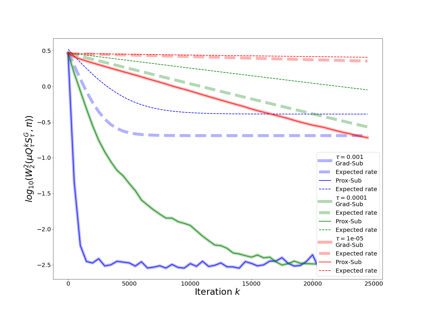
Refer to caption
Figure 1: Comparison of Grad-sub and Prox-sub for TVL2TVsuperscript𝐿2\operatorname*{TV}-L^{2} sampling in Wasserstein distance with σ=1𝜎1\sigma=1, λ=5𝜆5\lambda=5, τ=1e3,1e4,1e5𝜏1𝑒31𝑒41𝑒5\tau=1e-3,1e-4,1e-5. The color indicates the step size τ𝜏\tau, dashed lines the convergence rates obtained in the theory and solid lines the empirical ones, thick transparent lines the results from Grad-sub and thin lines the ones from Prox-sub.

Additionally, we also verify the convergence proven in Theorem 4.2 for the average distributions νkNsuperscriptsubscript𝜈𝑘𝑁\nu_{k}^{N} as defined in (4.16). This convergence holds identically for Grad-sub. We use no burn-in phase, that is N=0𝑁0N=0. The results are shown in Figure 2. Again, we note that the proven convergence rates are clearly exceeded with Prox-sub and Grad-sub performing almost identically.
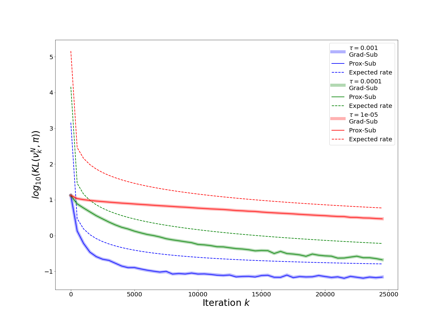
Refer to caption
Figure 2: Comparison of Grad-sub and Prox-sub for TVL2TVsuperscript𝐿2\operatorname*{TV}-L^{2} sampling in KL-divergence with σ=1𝜎1\sigma=1, λ=5𝜆5\lambda=5, τ=1e3,1e4,1e5𝜏1𝑒31𝑒41𝑒5\tau=1e-3,1e-4,1e-5. The color indicates the step size τ𝜏\tau, thick transparent lines the results from Grad-sub and thin lines the ones from Prox-sub. Dashed lines show the convergence rates obtained in the theory which are identical for both methods in this case.

In Figure 3 we compare the results of Prox-sub to the ones obtained with P-MALA [28] and MYULA [13]. For P-MALA a proposal for the update is computed as

X=proxτ(F+GK)(Xk)+2τBk+1.superscript𝑋subscriptprox𝜏𝐹𝐺𝐾subscript𝑋𝑘2𝜏subscript𝐵𝑘1X^{*}={\operatorname*{prox}}_{\tau(F+G\circ K)}(X_{k})+\sqrt{2\tau}B_{k+1}. (P-MALA)

Using a Metropolis-Hastings accept/reject step, this update is accepted for Xk+1subscript𝑋𝑘1X_{k+1} with probability min{1,π(X)q(Xk|X)π(Xk)q(X|Xk)}1𝜋superscript𝑋𝑞conditionalsubscript𝑋𝑘superscript𝑋𝜋subscript𝑋𝑘𝑞conditionalsuperscript𝑋subscript𝑋𝑘\min\left\{1,\frac{\pi(X^{*})q(X_{k}|X^{*})}{\pi(X_{k})q(X^{*}|X_{k})}\right\} and otherwise rejected leading to Xk+1=Xksubscript𝑋𝑘1subscript𝑋𝑘X_{k+1}=X_{k}. Here, q(x|y)=𝒩(x;proxτ(F+GK)(y),2τId)𝑞conditional𝑥𝑦𝒩𝑥subscriptprox𝜏𝐹𝐺𝐾𝑦2𝜏subscript𝐼𝑑q(x|y)=\mathcal{N}(x;{\operatorname*{prox}}_{\tau(F+G\circ K)}(y),2\tau I_{d}) with 𝒩(x;μ,Σ)𝒩𝑥𝜇Σ\mathcal{N}(x;\mu,\Sigma) being the density of a multivariate Gaussian with mean μ𝜇\mu and covariance matrix ΣΣ\Sigma evaluated at x𝑥x and Idd×dsubscript𝐼𝑑superscript𝑑𝑑I_{d}\in\mathbb{R}^{d\times d} denoting the unit matrix. One iteration of MYULA, on the other hand, is defined as

Xk+1=(1τθ)XkτF(Xk)+τθproxθGK(Xk)+2τBk+1subscript𝑋𝑘11𝜏𝜃subscript𝑋𝑘𝜏𝐹subscript𝑋𝑘𝜏𝜃subscriptprox𝜃𝐺𝐾subscript𝑋𝑘2𝜏subscript𝐵𝑘1X_{k+1}=(1-\frac{\tau}{\theta})X_{k}-\tau\nabla F(X_{k})+\frac{\tau}{\theta}{\operatorname*{prox}}_{\theta G\circ K}(X_{k})+\sqrt{2\tau}B_{k+1} (MYULA)

with a Moreau-Yoshida parameter θ>0𝜃0\theta>0 and the step size requirement τθθLF+1𝜏𝜃𝜃subscript𝐿𝐹1\tau\leq\frac{\theta}{\theta L_{\nabla F}+1}. In MYULA, the non-smooth part GK𝐺𝐾G\circ K is replaced by its differentiable Moreau envelope

(GK)θ(x)=minz12θzx2+G(Kz)superscript𝐺𝐾𝜃𝑥subscript𝑧12𝜃superscriptnorm𝑧𝑥2𝐺𝐾𝑧(G\circ K)^{\theta}(x)=\min\limits_{z}\frac{1}{2\theta}\|z-x\|^{2}+G(Kz) (7.1)

which approximates GK𝐺𝐾G\circ K as θ0𝜃0\theta\rightarrow 0. Applying standard ULA to the potential Uθ=F+(GK)θsuperscript𝑈𝜃𝐹superscript𝐺𝐾𝜃U^{\theta}=F+(G\circ K)^{\theta} leads to the above iteration which approximates the target density in total variation as θ0𝜃0\theta\rightarrow 0. For this experiment we set θ=0.01𝜃0.01\theta=0.01 yielding favorable convergence results. In Figure 3 we find very similar convergence behavior for P-MALA and MYULA. For P-MALA and MYULA convergence is proven in the TV-norm in [13, 28]. For Prox-sub convergence in TV is only guaranteed for the average distributions (νkN)ksubscriptsuperscriptsubscript𝜈𝑘𝑁𝑘(\nu_{k}^{N})_{k} which converge slower. However, as we could prove convergence of the iterates μQτkSτG𝜇subscriptsuperscript𝑄𝑘𝜏superscriptsubscript𝑆𝜏𝐺\mu Q^{k}_{\tau}S_{\tau}^{G} directly as well (albeit in Wasserstein distance) we also plot the TV distance of these iterates, which decreases at the same speed as for P-MALA and MYULA.
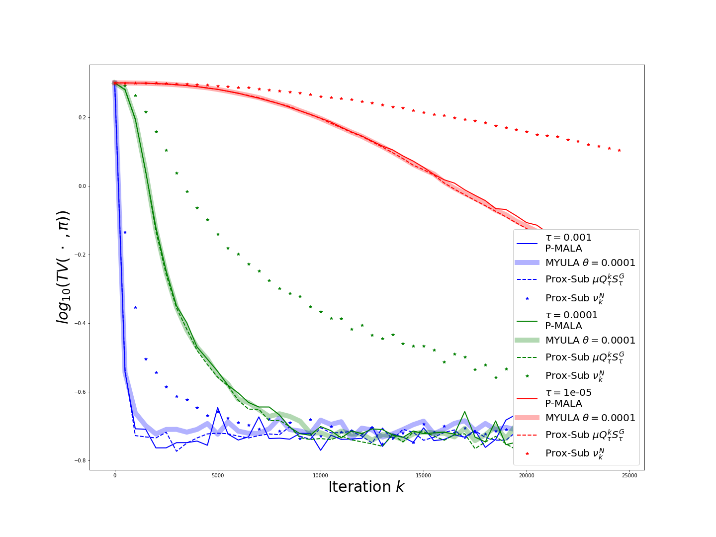
Refer to caption
Figure 3: Comparison of Prox-sub, P-MALA [28], and MYULA [13] for TVL2TVsuperscript𝐿2\operatorname*{TV}-L^{2} sampling in TV distance with σ=1𝜎1\sigma=1, λ=5𝜆5\lambda=5, τ=1e3,1e4,1e5𝜏1𝑒31𝑒41𝑒5\tau=1e-3,1e-4,1e-5. For Prox-sub we show both, the total variation distance of the iterates (νkN)ksubscriptsuperscriptsubscript𝜈𝑘𝑁𝑘(\nu_{k}^{N})_{k} for N=0𝑁0N=0 as well as for μQτkSτG𝜇subscriptsuperscript𝑄𝑘𝜏superscriptsubscript𝑆𝜏𝐺\mu Q^{k}_{\tau}S_{\tau}^{G}. For the former convergence is proven in TV whereas for the latter we could prove convergence in Wasserstein distance.

For P-MALA and MYULA iterative computation of the proximal mappings is necessary. We do so by employing the the primal-dual algorithm from [6] which we terminate when the difference between consecutive iterates is less than 1e41𝑒41e-4 in the maximum norm. This leads to an increased computational burden for these two methods. The computation times are listed in Table 7.1 for different step sizes. Interestingly, we find that in particular the computation time of P-MALA is sensitive to the step size. This is due to the fact, that the step size constitutes the prox-parameter in (P-MALA) with larger step sizes leading to more iterates within the primal-dual algorithm. For MYULA, on the other hand, the prox parameter is fixed as the hyperparameter θ𝜃\theta which is why the computation times are less sensitive to changes in the step-size. In several cases the proposed methods are even faster computing 1e4 parallel chains than P-MALA and MYULA computing a single chain which means that the total computational burden with the proposed methods is lower despite accounting the lack of ergodicity by running parallel chains instead of using consecutive samples of a single chain for estimation.

1e4 chains single chain
τ𝜏\tau P-MALA MYULA Grad-sub Prox-sub P-MALA MYULA Grad-sub Prox-sub
105superscript10510^{-5} 2.11 22.83 0.5 0.52 0.36 1.02 0.019 0.24
104superscript10410^{-4} 4.85 23.46 0.5 0.52 0.49 1.66 0.019 0.24
103superscript10310^{-3} 35.59 23.61 0.50 0.52 1.93 1.77 0.019 0.24
Table 7.1: Average computation times in seconds for 1000 iterations for different methods and step sizes τ𝜏\tau. We show the times for computing only a single Markov chain as well as for computation of 1e4 chains simultaneously in parallel.

Due to F𝐹F not being Lipschitz continuous, convergence of the subgradient method [10, Section 4.1] is not guaranteed. Nonetheless, since F𝐹F is locally Lipschitz and the iterates are typically bounded in practice, we apply the subgradient method (denoted by Sub in the sequel) as an additional comparison method. Note that for Sub, only convergence of the average distributions (νkN)ksubscriptsubscriptsuperscript𝜈𝑁𝑘𝑘(\nu^{N}_{k})_{k} can be expected, which is why we evaluate convergence of those average distributions. For Prox-sub on the other hand, we show the errors for both the iterates (νkN)ksubscriptsuperscriptsubscript𝜈𝑘𝑁𝑘(\nu_{k}^{N})_{k} as well as (μQτkSτG)ksubscript𝜇subscriptsuperscript𝑄𝑘𝜏subscriptsuperscript𝑆𝐺𝜏𝑘(\mu Q^{k}_{\tau}S^{G}_{\tau})_{k} itself, since we can ensure both to converge (albeit the latter in Wasserstein distance instead of KL). We employ the KL divergence between sampled and target distribution of Sub and Prox-sub as common metric to compare the convergence behavior as this is the metric where convergence is ensured for both methods, and also use a burn-in phase of N=0𝑁0N=0 for both methods. The results can be found in Figure 4. Evidently, averaging over successive distributions within the computation of νkNsubscriptsuperscript𝜈𝑁𝑘\nu^{N}_{k} leads to a slower convergence.

Refer to caption
Figure 4: Comparison of Prox-sub and Sub for TVL2TVsuperscript𝐿2\operatorname*{TV}-L^{2} sampling. For Prox-sub we show the KL divergence of both the iterates νkNsuperscriptsubscript𝜈𝑘𝑁\nu_{k}^{N} as well as μQτkSτG𝜇subscriptsuperscript𝑄𝑘𝜏subscriptsuperscript𝑆𝐺𝜏\mu Q^{k}_{\tau}S^{G}_{\tau}, for Sub of the iterates νkNsubscriptsuperscript𝜈𝑁𝑘\nu^{N}_{k} where the burn-in phase is set to N=0𝑁0N=0.

7.1.2 TVL1TVsuperscript𝐿1\operatorname*{TV}-L^{1} Sampling

The proposed method Prox-sub is also applicable in the case that F𝐹F is non-differentiable. As an example for this case we consider F𝐹F to be the L1superscript𝐿1L^{1} norm F:2:𝐹superscript2F:\mathbb{R}^{2}\rightarrow\mathbb{R} given as F(x)=1bxy1𝐹𝑥1𝑏subscriptnorm𝑥𝑦1F(x)=\frac{1}{b}\|x-y\|_{1} with b>0𝑏0b>0. Such a model is in particular reasonable working with data corrupted with noise following a Laplace distribution. This choice for F𝐹F is Lipschitz continuous with Lipschitz constant LF=b12subscript𝐿𝐹superscript𝑏12L_{F}=b^{-1}\sqrt{2}. Moreover, the proximal mapping of F𝐹F in this case reads as proxτF(x)=y+sign(xy)max{0,|xy|τb}subscriptprox𝜏𝐹𝑥𝑦sign𝑥𝑦0𝑥𝑦𝜏𝑏{\operatorname*{prox}}_{\tau F}(x)=y+\text{sign}(x-y)\max\{0,|x-y|-\frac{\tau}{b}\}. As before, we set y=(1,1)𝑦11y=(-1,1), b=1𝑏1b=1, and λ=5𝜆5\lambda=5. We compare the results of Prox-sub, and Sub, for which convergence can be ensured in this setting due to Lipschitz continuity of F𝐹F. Results are shown again for the step sizes τ=1e3,1e4,1e5𝜏1𝑒31𝑒41𝑒5\tau=1e-3,1e-4,1e-5. As before an estimated ground truth comparison target is obtained by computing the normalization constant Z=exp(F(x)G(Kx))dx𝑍𝐹𝑥𝐺𝐾𝑥d𝑥Z=\int\exp(-F(x)-G(Kx))\;\text{d}x by numerical integration and approximating the obtained density by a discretized distribution. We compute again 1e4 parallel Markov chains in this setting. The results are shown in Figure 5. Once again, both methods satisfy the proven convergence rates with barely a noticeable difference in convergence speed in practical experiments.
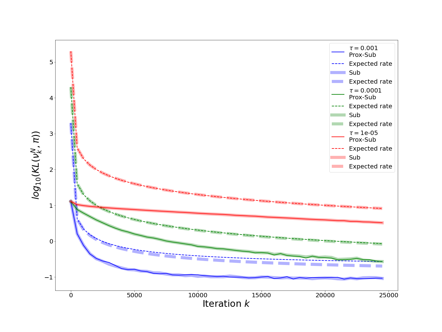
Refer to caption
Figure 5: Comparison of Prox-sub and Sub for TVL1TVsuperscript𝐿1\operatorname*{TV}-L^{1} sampling in KL-divergence with b=1𝑏1b=1, λ=5𝜆5\lambda=5, τ=1e3,1e4,1e5𝜏1𝑒31𝑒41𝑒5\tau=1e-3,1e-4,1e-5. The color indicates the step size τ𝜏\tau, dashed lines the convergence rates obtained in the theory and solid lines the empirical ones, thick transparent lines the results from Sub and thin lines the ones from Prox-sub.

We do not compare to P-MALA or MYULA as these methods are not particularly suited in this setting due to the necessary iterative computation of the proximal mapping of F+GK𝐹𝐺𝐾F+G\circ K for non-differentiable G𝐺G and F𝐹F.

7.2 Imaging Examples

In this section we show experimental results for applications in mathematical imaging. Since computing Wasserstein distances or KL-divergences between image samples constitutes a significant computational burden due to the high dimensionality, we do not compare entire distributions, but restrict ourselves to comparing expected values within the following experiments. Note that convergence of the error in expected values is a consequence of convergence in Wasserstein 2-distance. Indeed, given an optimal coupling (X,Y)𝑋𝑌(X,Y) for two distributions (μ,ν)𝜇𝜈(\mu,\nu), using Hölder’s inequality, we find

E[X]E[Y]22=E[XY]22E[XY22]=W22(μ,ν).subscriptsuperscriptnormE𝑋E𝑌22superscriptsubscriptnormE𝑋𝑌22Esuperscriptsubscriptnorm𝑋𝑌22subscriptsuperscript𝑊22𝜇𝜈\|\operatorname{E}[X]-\operatorname{E}[Y]\|^{2}_{2}=\|\operatorname{E}[X-Y]\|_{2}^{2}\leq\operatorname{E}[\|X-Y\|_{2}^{2}]=W^{2}_{2}(\mu,\nu).

In all imaging experiments, the functional G(Kx)𝐺𝐾𝑥G(Kx) is chosen to be the anisotropic total variation, that is G:2×n×m:𝐺superscript2𝑛𝑚G:\mathbb{R}^{2\times n\times m}\rightarrow\mathbb{R} and K:n×m2×n×m:𝐾superscript𝑛𝑚superscript2𝑛𝑚K:\mathbb{R}^{n\times m}\rightarrow\mathbb{R}^{2\times n\times m} are defined as G(p)=λp1=λi=1nj=1m|pi,j1|+|pi,j2|𝐺𝑝𝜆subscriptnorm𝑝1𝜆superscriptsubscript𝑖1𝑛superscriptsubscript𝑗1𝑚superscriptsubscript𝑝𝑖𝑗1superscriptsubscript𝑝𝑖𝑗2G(p)=\lambda\|p\|_{1}=\lambda\sum\limits_{i=1}^{n}\sum\limits_{j=1}^{m}|p_{i,j}^{1}|+|p_{i,j}^{2}| and

(Kx)i,j1={xi+1,jxi,jif i<n0else,(Kx)i2={xi,j+1xi,jif j<m0else.formulae-sequencesuperscriptsubscript𝐾𝑥𝑖𝑗1casessubscript𝑥𝑖1𝑗subscript𝑥𝑖𝑗if i<n0else,superscriptsubscript𝐾𝑥𝑖2casessubscript𝑥𝑖𝑗1subscript𝑥𝑖𝑗if j<m0else\displaystyle(Kx)_{i,j}^{1}=\begin{cases}x_{i+1,j}-x_{i,j}\quad&\text{if $i<n$}\\ 0\quad&\text{else,}\end{cases}\quad(Kx)_{i}^{2}=\begin{cases}x_{i,j+1}-x_{i,j}\quad&\text{if $j<m$}\\ 0\quad&\text{else}.\end{cases} (7.2)

We emphasize at this point that isotropic TV would be feasible as well. However, we use anisotropic TV since we want to compare our results to the ones obtained with Belief Propagation [27, 34, 18, 33], which is only applicable in the anisotropic case. The subdifferential of G𝐺G in this setting reads as

qG(p){qi,jk=λif pi,jk>0qi,jk=λif pi,jk<0qi,jk[λ,λ]if pi,jk=0𝑞𝐺𝑝casessuperscriptsubscript𝑞𝑖𝑗𝑘𝜆if superscriptsubscript𝑝𝑖𝑗𝑘0superscriptsubscript𝑞𝑖𝑗𝑘𝜆if superscriptsubscript𝑝𝑖𝑗𝑘0superscriptsubscript𝑞𝑖𝑗𝑘𝜆𝜆if superscriptsubscript𝑝𝑖𝑗𝑘0q\in\partial G(p)\Leftrightarrow\begin{cases}q_{i,j}^{k}=\lambda\quad&\text{if }p_{i,j}^{k}>0\\ q_{i,j}^{k}=-\lambda\quad&\text{if }p_{i,j}^{k}<0\\ q_{i,j}^{k}\in[-\lambda,\lambda]\quad&\text{if }p_{i,j}^{k}=0\end{cases} (7.3)

7.2.1 TVL2TVsuperscript𝐿2\operatorname*{TV}-L^{2} Denosing

As a first imaging example we consider TVL2TVsuperscript𝐿2\operatorname*{TV}-L^{2} denosing. That is, F:n×m:𝐹superscript𝑛𝑚F:\mathbb{R}^{n\times m}\rightarrow\mathbb{R} is defined as F(x)=12σ2xy22𝐹𝑥12superscript𝜎2superscriptsubscriptnorm𝑥𝑦22F(x)=\frac{1}{2\sigma^{2}}\|x-y\|_{2}^{2} for which the proximal mapping is analogous as in the two-dimensional case. As data yn×m𝑦superscript𝑛𝑚y\in\mathbb{R}^{n\times m} we use a ground truth image which is corrupted with additive Gaussian noise with mean zero and standard deviation σ=0.05𝜎0.05\sigma=0.05. The upper bound for the step size according to our theoretical results is σ2=0.0025superscript𝜎20.0025\sigma^{2}=0.0025 for both Grad-sub and Prox-sub. The scaling parameter λ𝜆\lambda from (7.2) is chosen as λ=30𝜆30\lambda=30. To obtain estimates of the ground truth for this setting we apply the Belief Propagation (BP) algorithm which yields highly accurate approximations of the marginal distributions of all image pixels, albeit for discrete gray-scale values. Specifically, we split the gray scale range of [0,1]01[0,1] into 100100100 evenly spaced values for the BP algorithm. Using the obtained marginal distributions we can compute the expected value as well as the pixel-wise marginal variances. For details on the application of BP to anisotropic TVL2TVsuperscript𝐿2\operatorname*{TV}-L^{2} denoising we refer the reader to [25, Sections 4.3, 5.1] and to the publicly available source code [17]. To compute the expected values for the samples generated with the proposed methods we run the algorithm for a burn in phase of N𝑁N iterations and then compute the mean of samples N+1,,N+k𝑁1𝑁𝑘N+1,\dots,N+k, which is denoted as x¯kNsubscriptsuperscript¯𝑥𝑁𝑘\bar{x}^{N}_{k}. Thus, in the high-dimensional setting, we additionally decrease the computational effort by avoiding the computation of large amounts of independent Markov chains and instead using successive samples of a single chain for estimation. While a proof of ergodicity of the proposed algorithms is outside the scope of this paper and left for future work, we note that different versions of the Ergodic Theorem state that under some conditions the mean of successive iterates of a Markov chain approximates the expected value of the stationary distribution of this chain despite the samples not being i.i.d. [16, Section 9.5], [29, Theorem 4.7.4]. Similarly to the mean, we use the same samples to compute the pixel-wise empirical variance. For all algorithms we use a burn-in phase of N=1e6𝑁1𝑒6N=1e6 iterations and afterwards deploy the following k=1e5𝑘1𝑒5k=1e5 samples.

In Figure 6 we show results for BP, MYULA, Grad-sub and Prox-sub with a step size of τ=1e5𝜏1𝑒5\tau=1e-5. The proximal mapping of GK𝐺𝐾G\circ K for MYULA is again computed iteratively using the primal-dual algorithm [6] which we terminate as soon as the update within the algorithm is less than 1e-4 in the maximum norm. Moreover, for MYULA we choose a Moreau-Yoshida parameter of θ=1e4𝜃1𝑒4\theta=1e-4 leading a reasonable trade-off of speed and approximation accuracy. While smaller values lead to a better approximation of the target density, they also force us to use smaller step sizes due to the requirement τθθLF+1𝜏𝜃𝜃subscript𝐿𝐹1\tau\leq\frac{\theta}{\theta L_{\nabla F}+1} which leads to slower convergence. Moreover, smaller θ𝜃\theta additionally increase the computational burden as they lead to a higher number of iterations within the primal-dual algorithm for computing the prox of GK𝐺𝐾G\circ K. We do not include numerical results for P-MALA as we could not achieve reasonable convergence. More specifically, in our experiments in order to achieve a reasonable acceptance rate of the Metropolis-Hastings step, the step size had to be chosen excessively small resulting in very slow convergence.

As expected we find high pixel-wise variances at the regions of jump discontinuities which is due to the very nature of the total variation functional penalizing sharp edges. Moreover, in Figure 7 we illustrate the squared L2superscript𝐿2L^{2} error to the BP results for the proposed methods and MYULA for different step sizes. Again, we observe that there is hardly any difference in accuracy between Prox-sub and Grad-sub probably due to the small step sizes. As previously, we see that accuracy increases as the step size decreases. As the remaining bias suffers from the curse of dimensions, the reached accuracy is worse compared to the 2D examples. It seems that MYULA yields a greater bias than the proposed methods. Unfortunately, reducing this bias by decreasing θ𝜃\theta would lead to smaller step sizes for MYULA and, thus, even slower convergence. Note that the accuracy of the reconstructed images compared to the clean images depends mostly on the model of the potential U𝑈U rather than the performance of the sampling algorithm. That is, a proficient sampling method should produce samples from π(x)exp(U(x))proportional-to𝜋𝑥𝑈𝑥\pi(x)\propto\exp(-U(x)) independent of how well this distribution is suited to acquire estimates of the unknown clean image. Therefore, we do not provide any results regarding the discrepancy of the MMSE estimates to the clean images as they do not provide any relevant information in the context of this research.

Refer to caption
Refer to captionRefer to caption
Refer to caption
Refer to captionRefer to caption
Figure 6: Expected values and marginal posterior variances for TVL2TVsuperscript𝐿2\operatorname*{TV}-L^{2} denoising computed with different methods. From left to right: Data y𝑦y, expected value computed with BP, MYULA, Grad-sub, Prox-sub, marginal variances computed with BP, MYULA, Grad-sub, Prox-sub. The proposed algorithms were performed with a step size of τ=1e5𝜏1𝑒5\tau=1e-5, a burn-in phase of N=1e6𝑁1𝑒6N=1e6 and the number of samples k=1e5𝑘1𝑒5k=1e5. The range of the image pixels was [0,1]01[0,1].
Refer to caption
Figure 7: Squared L2superscript𝐿2L^{2} error between the estimated expected values and the ones obtained via BP for the peppers image for denoising.

In Table 7.2 we provide the average computation times for 1000 iterations of image denoising (and deconvolution) with Grad-sub and Prox-sub compared to MYULA, where we again find that the iterative computation of the proximal mapping within MYULA significantly increases computational effort compared to the proposed method. However, it should be mentioned at this point that the use of consecutive samples is heuristic for Grad-sub and Prox-sub as ergodicity is not yet proven for these methods.

7.2.2 TVL2TVsuperscript𝐿2\operatorname*{TV}-L^{2} Deconvolution

As a second example in the field of imaging we provide an application including a non-trivial forward operator within the functional F𝐹F, namely image deconvolution. More precisely, F:n×m:𝐹superscript𝑛𝑚F:\mathbb{R}^{n\times m}\rightarrow\mathbb{R} is defined as F(x)=12σ2kxy22𝐹𝑥12superscript𝜎2superscriptsubscriptnorm𝑘𝑥𝑦22F(x)=\frac{1}{2\sigma^{2}}\|k*x-y\|_{2}^{2} where kx𝑘𝑥k*x denotes the convolution of x𝑥x with a convolution kernel ks×s𝑘superscript𝑠𝑠k\in\mathbb{R}^{s\times s}. While the application of Grad-sub does not constitute any difficulties as long as F𝐹F is differentiable, we require the computation of the proximal mapping of F𝐹F within Prox-sub. This is possible explicitly for this application since, in Fourier space, the convolution reduces to a pointwise multiplication with the Fourier transform of the convolution kernel, which renders the proximal mapping explicit. More precisely, using the facts that the Fourier transform is linear and unitary we find

proxτF(x)=1((𝟙+τσ2k^k^)1(x^+τσ2k^y^))subscriptprox𝜏𝐹𝑥superscript1direct-productsuperscript1direct-product𝜏superscript𝜎2^𝑘^𝑘absent1^𝑥direct-product𝜏superscript𝜎2^𝑘^𝑦{\operatorname*{prox}}_{\tau F}(x)=\mathcal{F}^{-1}\left((\mathbbm{1}+\frac{\tau}{\sigma^{2}}\hat{k}\odot\hat{k})^{\circ-1}\odot(\hat{x}+\frac{\tau}{\sigma^{2}}\hat{k}\odot\hat{y})\right)

where direct-product\odot denotes element-wise multiplication (Hadamard product), 𝟙1\mathbbm{1} a matrix with all entries set to one, k^^𝑘\hat{k} the discrete Fourier transform of k𝑘k and analogously for x,y𝑥𝑦x,y, A1superscript𝐴absent1A^{\circ-1} the element-wise inverse of a matrix A𝐴A, and 1superscript1\mathcal{F}^{-1} the inverse Fourier transform. Note that, the element-wise inverse is guaranteed to exist for τ𝜏\tau small enough. As a convolution kernel k𝑘k we use a Gaussian kernel of size s=5𝑠5s=5 normalized to integrate to 1. The data y is obtained as the convolution y=ku+σn𝑦𝑘𝑢𝜎𝑛y=k*u+\sigma n with a ground truth image u𝑢u and n𝑛n denoting pixel-wise standard Gaussian noise. We choose a noise level σ=0.01𝜎0.01\sigma=0.01. The scaling parameter λ𝜆\lambda from (7.2) is chosen as λ=20𝜆20\lambda=20. Since BP is not applicable in this setting, as a ground truth we apply Grad-sub with an added Metropolis-Hastings correction step, ensuring convergence to the stationary distribution [30], [29, Chapter 6]. Since it is not clear how long convergence to the stationary distribution takes using the Metropolis-Hastings correction, we use a significantly elongated burn-in phase of N=3e6𝑁3𝑒6N=3e6 iterations and compute mean and pixel-wise variances using the subsequent k=1e6𝑘1𝑒6k=1e6 samples to obtain our estimated ground truth comparison target. Again, we compare the proposed methods to MYULA for which we chose θ=1e4𝜃1𝑒4\theta=1e-4. Regarding the choice of θ𝜃\theta we refer the reader to the elaborations in Section 7.2.1. For Prox-sub and Grad-sub we use a burn-in phase of N=1e6𝑁1𝑒6N=1e6 iterations and the subsequent k=5e5𝑘5𝑒5k=5e5 samples. Visual results are depicted in Figure 8 for a step-size of τ=1e6𝜏1𝑒6\tau=1e-6 and convergence of the estimated expectation is illustrated in Figure 9, where x¯¯𝑥\bar{x} denotes the the expected value computed using the Metropolis-Hastings correction and x¯kNsubscriptsuperscript¯𝑥𝑁𝑘\bar{x}^{N}_{k} again the estimates based on the proposed methods. Keep in mind, however, that inaccuracies within the estimated ground truth obtained via the Metropolis-Hastings algorithm might additionally distort the accuracy.
Refer to caption
Refer to caption
Refer to caption
Refer to caption
Refer to caption
Refer to caption
Refer to caption
Refer to caption
Refer to caption
Refer to caption
Refer to caption
Refer to caption
Refer to caption
Refer to caption
Refer to caption
Refer to caption
Refer to caption
Refer to caption
Figure 8: Expected values and marginal posterior variances for TVL2TVsuperscript𝐿2\operatorname*{TV}-L^{2} deconvolution computed with different methods. From left to right: Data y𝑦y, expected value computed with Metropolis-Hastings correction, MYULA, Grad-sub, Prox-sub, marginal variances computed with Metropolis-Hastings correction, MYULA, Grad-sub, Prox-sub. The algorithms were performed with a step size of τ=1e6𝜏1𝑒6\tau=1e-6, a burn-in phase of N=1e6𝑁1𝑒6N=1e6 and the number of samples k=5e5𝑘5𝑒5k=5e5, the Metropolis-Hastings version with a burn-in phase of N=3e6𝑁3𝑒6N=3e6 and the number of samples k=1e6𝑘1𝑒6k=1e6. The range of the image pixels was [0,1]01[0,1].
Refer to caption
Figure 9: Squared L2superscript𝐿2L^{2} error between the estimated expected values using the proposed algorithms Grad-sub and Prox-sub and the ones obtained via the Metroplois-Hastings algorithm for the peppers image for deconvolution.

In Table 7.2 the computation times for image deconvolution for MYULA, Grad-sub, and Prox-sub are provided showing a similar result as above in that MYULA is computationally more expensive due to the iterative computation of proximal mappings.

denoising deconvolution
τ𝜏\tau MYULA Grad-sub Prox-sub MYULA Grad-sub Prox-sub
1e51𝑒51e-5 55.61 0.59 0.65 43.43 0.92 1.06
1e61𝑒61e-6 56.86 0.59 0.66 43.44 0.92 1.05
Table 7.2: Average computation times in seconds for 1000 iterations for different methods and step sizes τ𝜏\tau for image denoising.

8 Conclusion and Future Work

In this work we have proposed novel sampling algorithms for sampling from non-smooth densities of the form π(x)exp(F(x)G(Kx))similar-to𝜋𝑥𝐹𝑥𝐺𝐾𝑥\pi(x)\sim\exp(-F(x)-G(Kx)) with functionals F,G𝐹𝐺F,G and a linear operator K𝐾K. The methods are in particular applicable in the setting that G𝐺G is non-differentiable, and, for the first time, allow sampling with guaranteed convergence in applications with F𝐹F not being Lipschitz continuous. We have proven several non-asymptotic convergence results where convergence is obtained in the Kullback-Leibler divergence if F𝐹F is non-differentiable and in Wasserstein 2-distance with a faster rate in the case of stronger regularity assumptions on F𝐹F. The presented experimental results confirm the proven convergence rates and provide empirical evidence of the practical relevance of the proposed methods in the field of Bayesian imaging.

Future Work

An important issue to address in future work is existence and uniqueness of stationary measures for the proposed transition kernels Rτ~,τsubscript𝑅~𝜏𝜏R_{\tilde{\tau},\tau} and, consequently, ergodicity of the resulting Markov chain which constitutes a difficult question due to the non-differentiability of the target density π𝜋\pi. However, such results could reduce the computational complexity as it would obviate the need for running multiple Markov chains for the estimation of statistics of the target density π𝜋\pi. This is due to the fact that ergodic theorems [24, Chapter 17] allow us to work with the running mean of a single chain instead of the mean over independent chains.

Another interesting line of possible future work concerns convergence guarantees of a primal-dual sampling algorithm inspired by [7], as was for instance used in [25] without proving convergence. The possibility of avoiding step size constraints, similar to primal-dual minimization techniques, could provide a significant increase in speed of convergence.

References

  • [1] Pascal Bianchi, Adil Salim and Sholom Schechtman “Passty Langevin” In Conference on Machine Learning (CAp), 2019
  • [2] François Bolley, Ivan Gentil and Arnaud Guillin “Convergence to equilibrium in Wasserstein distance for Fokker–Planck equations” In Journal of Functional Analysis 263.8 Elsevier, 2012, pp. 2430–2457
  • [3] Kristian Bredies and Martin Holler “Higher-order total variation approaches and generalisations” In Inverse Problems. Topical Review 36.12, 2020, pp. 123001
  • [4] Nicolas Brosse, Alain Durmus, Éric Moulines and Marcelo Pereyra “Sampling from a log-concave distribution with compact support with proximal Langevin Monte Carlo” In Conference on learning theory, 2017, pp. 319–342 PMLR
  • [5] Xiaohao Cai, Jason D McEwen and Marcelo Pereyra “Proximal nested sampling for high-dimensional Bayesian model selection” In Statistics and Computing 32.5 Springer, 2022, pp. 87
  • [6] Antonin Chambolle and Thomas Pock “A first-order primal-dual algorithm for convex problems with applications to imaging” In Journal of Mathematical Imaging and Vision 40 Springer US, 2011, pp. 120–145 DOI: 10.1007/s10851-010-0251-1
  • [7] Antonin Chambolle and Thomas Pock “On the ergodic convergence rates of a first-order primal–dual algorithm” In Mathematical Programming 159.1-2 Springer, 2016, pp. 253–287
  • [8] Yongxin Chen, Sinho Chewi, Adil Salim and Andre Wibisono “Improved analysis for a proximal algorithm for sampling” In Proceedings of Thirty Fifth Conference on Learning Theory 178, Proceedings of Machine Learning Research PMLR, 2022, pp. 2984–3014 URL: https://proceedings.mlr.press/v178/chen22c.html
  • [9] Arnak S Dalalyan “Theoretical guarantees for approximate sampling from smooth and log-concave densities” In Journal of the Royal Statistical Society Series B: Statistical Methodology 79.3 Oxford University Press, 2017, pp. 651–676
  • [10] Alain Durmus, Szymon Majewski and Błażej Miasojedow “Analysis of Langevin Monte Carlo via convex optimization” In The Journal of Machine Learning Research 20.1 JMLR. org, 2019, pp. 2666–2711
  • [11] ALAIN DURMUS and ÉRIC MOULINES “High-dimensional Bayesian inference via the unadjusted Langevin algorithm” In Bernoulli 25.4A, 2019, pp. 2854–2882
  • [12] Alain Durmus and Éric Moulines “Nonasymptotic convergence analysis for the unadjusted Langevin algorithm” In Annals of Applied Probability 27.3, 2017, pp. 1551–1587
  • [13] Alain Durmus, Éric Moulines and Marcelo Pereyra “A Proximal Markov Chain Monte Carlo Method for Bayesian Inference in Imaging Inverse Problems: When Langevin Meets Moreau” In SIAM Review 64.4 SIAM, 2022, pp. 991–1028
  • [14] Matthias J Ehrhardt, Lorenz Kuger and Carola-Bibiane Schönlieb “Proximal Langevin Sampling With Inexact Proximal Mapping” In arXiv preprint arXiv:2306.17737, 2023
  • [15] Rémi Flamary, Nicolas Courty, Alexandre Gramfort, Mokhtar Z Alaya, Aurélie Boisbunon, Stanislas Chambon, Laetitia Chapel, Adrien Corenflos, Kilian Fatras and Nemo Fournier “Pot: Python optimal transport” In The Journal of Machine Learning Research 22.1 JMLRORG, 2021, pp. 3571–3578
  • [16] Geoffrey Grimmett and David Stirzaker “Probability and random processes” Oxford university press, 2020
  • [17] Andreas Habring, Martin Holler and Thomas Pock “Source code to reproduce the results of ”Subgradient Langevin Methods for Sampling from Non-smooth Potentials”” In GitHub repository GitHub, https://github.com/habring/subgradient_langevin, 2023
  • [18] Patrick Knobelreiter, Christian Sormann, Alexander Shekhovtsov, Friedrich Fraundorfer and Thomas Pock “Belief propagation reloaded: Learning bp-layers for labeling problems” In Proceedings of the IEEE/CVF Conference on Computer Vision and Pattern Recognition, 2020, pp. 7900–7909
  • [19] Damien Lamberton and Gilles Pages “Recursive computation of the invariant distribution of a diffusion: the case of a weakly mean reverting drift” In Stochastics and dynamics 3.04 World Scientific, 2003, pp. 435–451
  • [20] Rémi Laumont, Valentin De Bortoli, Andrés Almansa, Julie Delon, Alain Durmus and Marcelo Pereyra “Bayesian imaging using plug & play priors: when langevin meets tweedie” In SIAM Journal on Imaging Sciences 15.2 SIAM, 2022, pp. 701–737
  • [21] Yin Tat Lee, Ruoqi Shen and Kevin Tian “Structured Logconcave Sampling with a Restricted Gaussian Oracle” In Proceedings of Thirty Fourth Conference on Learning Theory 134, Proceedings of Machine Learning Research PMLR, 2021, pp. 2993–3050 URL: https://proceedings.mlr.press/v134/lee21a.html
  • [22] Jiaming Liang and Yongxin Chen “A Proximal Algorithm for Sampling from Non-Smooth Potentials” In 2022 Winter Simulation Conference (WSC), 2022, pp. 3229–3240 DOI: 10.1109/WSC57314.2022.10015293
  • [23] Tung Duy Luu, Jalal Fadili and Christophe Chesneau “Sampling from Non-smooth Distributions Through Langevin Diffusion” In Methodology and Computing in Applied Probability 23.4, 2021, pp. 1173–1201 DOI: 10.1007/s11009-020-09809-7
  • [24] Sean P Meyn and Richard L Tweedie “Markov chains and stochastic stability” Springer Science & Business Media, 2012
  • [25] Dominik Narnhofer, Andreas Habring, Martin Holler and Thomas Pock “Posterior-variance-based error quantification for inverse problems in imaging” In arXiv preprint arXiv:2212.12499, 2022
  • [26] Giorgio Parisi “Correlation functions and computer simulations” In Nuclear Physics B 180.3 Elsevier, 1981, pp. 378–384
  • [27] J. Pearl “Reverend Bayes on inference engines: A distributed hierarchical approach” In Proceedings AAAI Natinal Conference on AI, 1982, pp. 133–136
  • [28] Marcelo Pereyra “Proximal markov chain monte carlo algorithms” In Statistics and Computing 26 Springer, 2016, pp. 745–760
  • [29] Christian P Robert, George Casella and George Casella “Monte Carlo statistical methods” Springer, 1999
  • [30] Gareth O Roberts and Richard L Tweedie “Exponential convergence of Langevin distributions and their discrete approximations” In Bernoulli JSTOR, 1996, pp. 341–363
  • [31] Peter J Rossky, Jimmie D Doll and Harold L Friedman “Brownian dynamics as smart Monte Carlo simulation” In The Journal of Chemical Physics 69.10 American Institute of Physics, 1978, pp. 4628–4633
  • [32] Leonid I. Rudin, Stanley Osher and Emad Fatemi “Nonlinear total variation based noise removal algorithms” In Physica D 60.1–4, 1992, pp. 259–268
  • [33] Richard Szeliski, Ramin Zabih, Daniel Scharstein, Olga Veksler, Vladimir Kolmogorov, Aseem Agarwala, Marshall Tappen and Carsten Rother “A comparative study of energy minimization methods for markov random fields with smoothness-based priors” In IEEE transactions on pattern analysis and machine intelligence 30.6 IEEE, 2008, pp. 1068–1080
  • [34] Marshall F Tappen and Freeman William T. “Comparison of graph cuts with belief propagation for stereo, using identical MRF parameters” In Proceedings Ninth IEEE International Conference on Computer Vision, 2003, pp. 900–906 vol.2
  • [35] Tuomo Valkonen “Testing and non-linear preconditioning of the proximal point method” In Applied Mathematics & Optimization 82.2 Springer, 2020, pp. 591–636
  • [36] Cédric Villani “Optimal transport: old and new” Springer, 2009
  • [37] Maxime Vono, Nicolas Dobigeon and Pierre Chainais “Split-and-Augmented Gibbs Sampler—Application to Large-Scale Inference Problems” In IEEE Transactions on Signal Processing 67.6, 2019, pp. 1648–1661 DOI: 10.1109/TSP.2019.2894825
  • [38] Maxime Vono, Daniel Paulin and Arnaud Doucet “Efficient MCMC sampling with dimension-free convergence rate using ADMM-type splitting” In J. Mach. Learn. Res. 23.1 JMLR.org, 2022
  • [39] Martin Zach, Florian Knoll and Thomas Pock “Stable deep MRI reconstruction using Generative Priors” In arXiv preprint arXiv:2210.13834, 2022
  • [40] Martin Zach, Erich Kobler and Thomas Pock “Computed Tomography reconstruction using generative energy-based priors” In arXiv preprint arXiv:2203.12658, 2022
  • [41] Song Chun Zhu, Ying Nian Wu and David Mumford “Minimax entropy principle and its application to texture modeling” In Neural computation 9.8 MIT Press, 1997, pp. 1627–1660