A Universal Birkhoff Theory for Fast Trajectory Optimization

Abstract

Over the last two decades, pseudospectral methods based on Lagrange interpolants have flourished in solving trajectory optimization problems and their flight implementations. In a seemingly unjustified departure from these highly successful methods, a new starting point for trajectory optimization is proposed. This starting point is based on the recently-developed concept of universal Birkhoff interpolants. The new approach offers a substantial computational upgrade to the Lagrange theory in completely flattening the rapid growth of the condition numbers from $\mathcal{O}(N^{2})$ to $\mathcal{O}(1)$, where $N$ is the number of grid points. In addition, the Birkhoff-specific primal-dual computations are isolated to a well-conditioned linear system even for nonlinear, nonconvex problems. This is part I of a two-part paper. In part I, a new theory is developed on the basis of two hypotheses. Other than these hypotheses, the theoretical development makes no assumptions on the choices of basis functions or the selection of grid points. Several covector mapping theorems are proved to establish the mathematical equivalence between direct and indirect Birkhoff methods. In part II of this paper (with Proulx), it is shown that a select family of Gegenbauer grids satisfy the two hypotheses required for the theory to hold. Numerical examples in part II illustrate the power and utility of the new theory.

1 Introduction

Barring a few exceptions, trajectory optimization problems are open-loop optimal control problems[3, 2, 1, 4]. If a solution to a trajectory optimization problem can be computed in “real time,” then optimal feedback control is possible[1, 6, 5, 7] without a need to solve the difficult Hamilton-Jacobi-Bellman equations[8, 10, 9]. But what exactly is real time? Intuitively, it is apparent that if a dynamical system is “slow” then the time to recompute an optimal open-loop control can be large. Conversely, a faster dynamical system necessitates a faster computational speed to achieve the same closed-loop-objectives of a slower system. This intuitive concept is made rigorous in [6] and [11] in terms of the Lipschitz constant[9, 10] of a dynamical system. That is, if a solution to a trajectory optimization problem is computed at a rate faster than the Lipschitz frequency[1, 6] of the dynamical system, then the computational speed is termed real-time[1, 6, 11]. This foundational concept of real-time is agnostic to computational hardware; in fact, it levies the requirements for pairing a computing system to a specific dynamical system. On the basis of this definition, real-time optimal control (RTOC) was used in [11] to stabilize an otherwise-unstable inverted pendulum without explicitly constructing a feedback controller. It was also used in [6] to ground-test various optimal feedback slew maneuvers for NPSAT1, an experimental satellite built at the Naval Postgraduate School and launched in June 2019. These engineering applications demonstrated the practical use of the theoretical concept of using the Lipschitz frequency to define RTOC. The concept of RTOC facilitates the construction of a closed-loop control system without the requirement for producing a closed-form solution to a feedback control law[1]. Because a traditional closed-form feedback controller automatically implies real-time computation, it is apparent that real-time computation is more fundamental to the production of closed-loop controllers than “analytical expressions” of a control function in terms of state variables. Note that RTOC does not mean traditional closed-form feedback controls must be abandoned. In fact, as described in [1], RTOC can be used in concert with heritage control systems as an enabling technology for designing various outer-loops under the rubric of different guidance and control system architectures[12].

It is important to recognize that application-specific RTOC algorithms are not new; they have been used for quite some time in the aerospace industry under the heading of closed-loop guidance[1, 14, 13, 7, 5]. For example, the well-known powered explicit guidance[13] is a closed-loop application of the optimal open-loop linear tangent equation[8, 1]. Many more application-specific RTOC algorithms have been developed in recent years[14, 7, 5]. General-purpose RTOC-based feedback controllers are, relatively, more recent developments[1, 6]. As shown in[6, 15, 16, 17, 18, 19, 20, 21], the same general-purpose trajectory optimization method used to stabilize an inverted pendulum in [11] was reused multiple times, without change, to generate attitude guidance commands for NPSAT1[6], entry guidance algorithms for hypersonic vehicles[15, 16], autonomous operations of ground robots in cluttered and uncertain environments[17, 18], cooperative controls for multiple uninhabited aerial vehicles[19], and other disparate applications[20, 21]. The common theme in all these diverse applications was pseudospectral (PS) optimal control theory[22]. One of the primary reasons for using PS optimal control theory for RTOC (as a general-purpose approach) is their near-exponential rate of convergence[23, 24]. That is, it takes relatively few grid points to generate an accurate trajectory solution and even fewer points to close the loop[6, 11, 26, 25]. The latter result is due to the anti-aliasing phenomenon of the ensuing Bellman PS effect[25, 26, 27]. For problems where there is a need for a highly dense grid, the theoretical fast rate of convergence of a PS method is practically dampened by round-off errors[28, 29] and the rapidly increasing condition number of the resulting linear algebra that underpins the trajectory optimization algorithm[30, 31, 32, 33]. The latter point is illustrated in Fig. 1 which shows the $\mathcal{O}(N^{2})$ growth in the condition number of a PS method, where $N$ is the number of grid points.

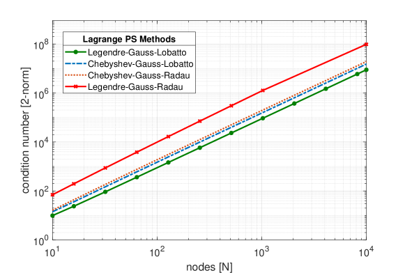
Figure 1: $\mathcal{O}(N^{2})$ growth in the condition number of a Lagrange PS method for various choices of grid selections; data from [34].

To mitigate the impact of high condition numbers, preconditioners are commonly used[35, 36] to “bend the curve” of Fig. 1. Up until the pioneering work of Wang et al[37], the best preconditioner generated $\mathcal{O}(\sqrt{N})$ condition numbers (caveated by certain technical conditions[35, 36, 37]). As impressive as $\mathcal{O}(\sqrt{N})$ is, the research of Wang et al[37] changed everything; in fact, it was revolutionary. This is because:

1. It solved the long-standing problem[35, 36, 37] of finding the computationally perfect preconditioners in generating $\mathcal{O}(1)$ condition numbers; and,

2. It opened the door for abandoning the use of Lagrange interpolants as a starting point for all PS methods[38, 39, 29]; i.e., it effectively made all prior PS methods “obsolete.”

As a result of the first aforementioned point, fast and accurate solutions to boundary value problems (BVPs) became possible using the perfect preconditioner. Nonetheless, it is the second point that made the work of Wang et al[37] quite revolutionary. This is because they showed how a PS theory could be conceived from a new starting point. That is, instead of using Lagrange interpolants and subsequent preconditioners to formulate a fast PS method, Wang et al[37] showed that the better starting point was a Birkhoff interpolant[40, 41]. This essentially rendered all prior methods obsolete. Thus, if a PS method were to be introduced using Birkhoff interpolants, then many of the challenges associated with Lagrange interpolants vanish in one fell swoop. Furthermore, because high condition numbers are anathema to both computational speed and accuracy, the resulting well-conditioned Birkhoff PS methods are capable of generating fast and accurate solutions over thousands of grid points[37, 34]. Thus, a Birkhoff PS method, if applied to trajectory optimization, offers itself as a prime practical candidate for a general-purpose RTOC method to solve nonlinear, nonconvex aerospace guidance problems. This paper advances the foundations of such methods through the use of the new universal Birkhoff interpolants proposed in [42]. These universal Birkhoff interpolants are different from those of Wang el al[37] in several different ways[42] and offer many theoretical and practical advantages, particularly in dual space.

A Birkhoff interpolant[40, 41] allows a heterogenous mix of derivatives of various orders as part of its constituent elements. In [37], Wang et al showed that a careful selection of this mixture can be used to generate a family of fast and accurate methods for solving a variety of BVPs. Motivated by their ground breaking work, we adapted the ideas of Wang et al[37] for solving trajectory optimization problems[34, 43]. Although trajectory optimization problems may be viewed as generators of BVPs, an adaption of [37] to solve optimal control problems proved to be not entirely straightforward[34, 43]. This is because [37] requires a production of different Birkhoff interpolants for different BVPs based on their order and the type of boundary conditions such as Dirichlet, Neumann or Robin. In seeking a more universal approach, we advanced in [42] a new family of Birkhoff interpolants that eliminate the need for such specialized treatments. These universal Birkhoff interpolants address BVPs of various orders and mixtures of boundary conditions without the need to redevelop the method for different problems. In this two-part paper, we further these ideas to develop a new approach for solving general-purpose trajectory optimization problems. Part II of this paper is [44].

In this paper (i.e., Part I), we show that the new Birkhoff interpolants satisfy the covector mapping principle (CMP)[1, 4, 45, 46] under certain hypotheses pertaining to the selection of grid points. These hypotheses are shown to satisfy in part II of this paper when the grid is selected from a family of Gegenbauer node points. A satisfaction of the CMP by any discretization method has major ramifications on trajectory optimization. This is because the CMP implies the following[1, 4, 30, 33, 47]:

1. The oft quoted distinctions[3, 48, 49] between a direct and indirect method vanishes[1, 4];

2. An equivalence between a direct and indirect method can be advantageously used for the production of significantly faster algorithms[30, 33];

3. Every computed solution for a specific problem can be readily tested for optimality by simple checks of key necessary conditions resulting from an application of Pontryagin’s Principle[1, 33, 44]; and,

4. If a problem is badly scaled because of the use of engineering units, it can be quickly re-scaled for computational speed and accuracy by employing the concept of (non-canonical) designer units[1, 47] made possible by covector balancing techniques[47].

Taken all together, the promise of a universal Birkhoff PS theory for trajectory optimization with applications to RTOC is as follows:

1. The near-exponential rate of convergence of PS theory remains intact when the Lagrange interpolant is replaced by a Birkhoff interpolant. This fact implies the resulting scale of the Birkhoff-PS-discretized mathematical programming problem continues to be “exponentially smaller” when compared to non-PS methods[50];

2. The growth in the condition numbers of the linear algebra that underpins the resulting trajectory optimization algorithm is flattened to $\mathcal{O}(1)$ (or $\mathcal{O}(\sqrt{N})$; see [44]). This fact implies one can generate fast and accurate solutions;

3. Round-off errors[28, 37] that plague the production of large differentiation matrices vanish in one fell swoop. This is because the Birkhoff matrices can be computed over thousands of grid points in a fast and stable manner[37, 42];

4. Coupled with recent advancements in spectral methods[51, 54, 52, 53], even millions of grid points can be generated at an $\mathcal{O}(1)$ computational speed. This fact implies grid refinement can be performed “instantaneously[34].”

2 New Mathematical Foundations of Birkhoff Interpolants

As noted elsewhere[34, 43, 55, 56], the development of a PS method using a Gaussian grid at the outset tends to obfuscate an otherwise clear idea. Consequently, we follow [43, 56] and use an arbitrary grid as a starting point. More importantly, the use of an arbitrary grid and possibly non-orthogonal, non-polynomial basis functions[57] generates a simpler and more elegant theory. Furthermore, the use of an arbitrary grid for the development of a PS theory explains when and why a Gaussian condition or orthogonality is imposed[56, 43]. Note also that a Gaussian grid is neither necessary nor critical for convergence[56]. With these observations in focus, we begin by defining

$$\pi^{N}:=\left\{\tau_{0},\tau_{1},\ldots,\tau_{N}\right\},\quad\tau_{k}\in\mathbb{R},\ k\in\mathbb{N}$$ (1)

to be a set of arbitrary grid points (see Fig. 2) over the time interval $[\tau^{a},\tau^{b}]$ such that

$$-\infty<\tau^{a}\leq\tau_{0}<\tau_{1}<\cdots<\tau_{N-1}<\tau_{N}\leq\tau^{b}<\infty$$ (2)

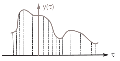
Figure 2: Schematic for an arbitrary grid; adapted from [56, 43].

For the purposes of simplicity in the presentation of the ideas, we assume a finite horizon while noting that the results presented in [58, 59, 11] easily allow its extension to infinite-horizon problems; see also [1] and the references contained therein for additional details pertaining to solving infinite-horizon problems.

Let, $[\tau^{a},\tau^{b}]\ni\tau\mapsto y(\tau)\in\mathbb{R}$ be a given differentiable function. In [42], we defined two Birkhoff interpolants (over the same grid, $\pi^{N}$) given by,

$$I^{N}_{a}y(\tau) :=y(\tau^{a})B_{0}^{0}(\tau)+\sum_{j=0}^{N}\dot{y}(\tau_{j})B_{j}^{a}(\tau)$$ (3a)

$$I^{N}_{b}y(\tau) :=\sum_{j=0}^{N}\dot{y}(\tau_{j})B_{j}^{b}(\tau)+y(\tau^{b})B_{N}^{N}(\tau)$$ (3b)

where, $I^{N}_{\theta},\theta\in\left\{a,b\right\}$ are the two interpolation operators and $B_{j}^{\theta},\ \theta\in\left\{a,b\right\},j=0,\ldots,N$ are (Birkhoff) basis functions that satisfy the interpolation conditions,

$$\begin{aligned} &B_{0}^{0}(\tau^{a})&=1,&&&B_{N}^{N}(\tau^{b})&&=1,\\ &{\dot{B}}_{0}^{0}(\tau_{i})&=0,&&&{\dot{B}}_{N}^{N}(\tau_{i})&&=0,&i=0,\ldots,N\\ &B_{j}^{a}(\tau^{a})&=0,&&&B_{j}^{b}(\tau^{b})&&=0,\qquad\qquad&j=0,\ldots,N\\ &{\dot{B}}_{j}^{\theta}(\tau_{i})&=\delta_{ij},&&&&&&i=0,\ldots,N,\ j=0,\ldots,N\end{aligned}$$ (4)

and $\delta_{ij}$ is the Kronecker delta.

Remark 1

Equation (4) is obtained by simply imposing the interpolation conditions,

$$I^{N}_{a}y(\tau^{a}) =y(\tau^{a}), \left.\frac{d}{d\tau}\left(I^{N}_{a}y(\tau)\right)\right|_{\tau=\tau_{j}}=\dot{y}(\tau_{i}), i=0,\ldots,N$$ (5a)

$$I^{N}_{b}y(\tau^{b}) =y(\tau^{b}), \left.\frac{d}{d\tau}\left(I^{N}_{b}y(\tau)\right)\right|_{\tau=\tau_{j}}=\dot{y}(\tau_{i}), i=0,\ldots,N$$ (5b)

Remark 2

There is no assumption of polynomials in all of the preceding equations.

Remark 3

In principle, one can define an additional family of $(N+1)$ different Birkhoff interpolants over the exact same grid $\pi^{N}$ (and not just two) by replacing $y(\tau^{a})$ in (3a) by $y(\tau_{k}),k=0,1,\ldots,N$.

Unlike Lagrange or Hermite interpolants, a Birkhoff interpolant might not exist[40, 41]; hence, it is critically important to prove its existence at the outset.

Lemma 1 (Existence and Uniqueness Lemma[42])

Let $L_{j}(\tau)$ be the antiderivative of $\ell_{j}(\tau)$, the $j$th Lagrange interpolating basis function over $\pi^{N}$. Then, the Birkhoff basis functions that satisfy (4) are given explicitly by,

$$B^{0}_{0}(\tau) =1=B^{N}_{N}(x)$$ (6a)

$$B_{j}^{a}(\tau) =L_{j}(\tau)-L_{j}(\tau^{a}), j=0,\ldots,N$$ (6b)

$$B_{j}^{b}(\tau) =L_{j}(\tau)-L_{j}(\tau^{b}), j=0,\ldots,N$$ (6c)

As noted in [42], these Birkhoff interpolants are different from the ones developed by Wang et al[37] but enjoy many of the same desirable properties. They are shown to be universal in [42] in the sense that they can be applied without change to solve high-order differential equations and a variety of boundary conditions, such as Dirichlet, Neumann and Robin. It will be apparent shortly that they are also universal in their applications to trajectory optimization.

Definition 1 ([42])

The Birkhoff quadrature weights, $w^{B}_{j},\ j=0,\ldots,N$, are defined by,

$$w^{B}_{j}:=\int_{\tau_{a}}^{\tau_{b}}\ell_{j}(\tau)\,d\tau$$ (7)

Lemma 2 ([42])

$\big{(}B^{a}_{j}(\tau)-B^{b}_{j}(\tau)\big{)}$ is a constant given by,

$$B^{a}_{j}(\tau)-B^{b}_{j}(\tau)=w^{B}_{j}$$ (8)

Definition 2

The $a$- and $b$-forms of the Birkhoff interpolants for $y(\tau)$ given by (3) are said to be equivalent if $I^{N}_{a}y(\tau)=I^{N}_{b}y(\tau)\ \forall\tau\in[\tau^{a},\tau^{b}]$.

Proposition 1

The $a$- and $b$-forms of the Birkhoff interpolants given by (3) are equivalent if and only if

$$y(\tau^{b})=y(\tau^{a})+\sum_{j=0}^{N}w^{B}_{j}\,{\dot{y}}(\tau_{j})$$ (9)

Proof 2.1.

We will first prove that if $I^{N}_{a}y(\tau)=I^{N}_{b}y(\tau)\ \forall\tau\in[\tau^{a},\tau^{b}]$, then (9) holds.

Equating (3a) and (3b) we get,

$$y(\tau^{a})B_{0}^{0}(\tau)+\sum_{j=0}^{N}\dot{y}(\tau_{j})B_{j}^{a}(\tau)=\sum_{j=0}^{N}\dot{y}(\tau_{j})B_{j}^{b}(\tau)+y(\tau^{b})B_{N}^{N}(\tau)$$ (10)

Equation (9) then follows from Lemma 2 and (6a).

To prove the converse, substitute (9) in (3b). This generates,

$$I^{N}_{b}y(\tau) :=\sum_{j=0}^{N}\dot{y}(\tau_{j})B_{j}^{b}(\tau)+y(\tau^{b})B_{N}^{N}(\tau)$$

$$=\sum_{j=0}^{N}\dot{y}(\tau_{j})B_{j}^{b}(\tau)+y(\tau^{a})B_{N}^{N}(\tau)+\sum_{j=0}^{N}w^{B}_{j}\,{\dot{y}}(\tau_{j})B_{N}^{N}(\tau)$$

$$=\sum_{j=0}^{N}\dot{y}(\tau_{j})B_{j}^{b}(\tau)+y(\tau^{a})B_{0}^{0}(\tau)+\sum_{j=0}^{N}(B^{a}_{j}(\tau)-B^{b}_{j}(\tau))\,{\dot{y}}(\tau_{j})$$ (11)

where, the last equation follows from Lemma 2 and (6a). Simplifying (11) yields $I^{N}_{b}y(\tau)=y(\tau^{a})B_{0}^{0}(\tau)+\sum_{j=0}^{N}B^{a}_{j}(\tau)\,\dot{y}(\tau_{j})=I^{N}_{a}y(\tau)$, by definition (cf. (3a)).

Definition 2.2 ([42]).

Let $\theta\in\left\{a,b\right\}$. The Birkhoff matrix, ${\boldsymbol{B}}^{\theta}$, is defined by,

$${\boldsymbol{B}}^{\theta}=\begin{bmatrix}B_{0}^{\theta}(\tau_{0})&B_{1}^{\theta}(\tau_{0})&\dots&B_{N}^{\theta}(\tau_{0})\\ B_{0}^{\theta}(\tau_{1})&B_{1}^{\theta}(\tau_{1})&\dots&B_{N}^{\theta}(\tau_{1})\\ \vdots&\vdots&&\vdots\\ B_{0}^{\theta}(\tau_{N})&B_{1}^{\theta}(\tau_{N})&\dots&B_{N}^{\theta}(\tau_{N})\end{bmatrix}$$ (12)

Definition 2.3.

2. The $(N+1)$ Birkhoff quadrature weight vector is defined by ${\boldsymbol{w}}_{B}:=[w^{B}_{0},\ldots,w^{B}_{N}]^{T}$

3. The $(N+1)\times(N+1)$ Birkhoff quadrature weight matrix is defined by $W_{B}:=\textrm{diag}(w^{B}_{0},\ldots,w^{B}_{N})$

Lemma 2.4 ([42] ).

Suppose $\pi^{N}$ is such that $\tau_{0}=\tau^{a}$ and $\tau_{N}=\tau_{b}$. Then,

1. The last row of ${\boldsymbol{B}}^{a}$ is identically equal to the Birkhoff quadrature weights.

2. The first row of ${\boldsymbol{B}}^{b}$ is identically equal to the negative of the Birkhoff quadrature weights.

Remark 2.5.

Lemma 2.4 implies that if $\pi^{N}$ is selected such that $\tau_{0}=\tau^{a}$ and $\tau_{N}=\tau_{b}$, then the Birkhoff quadrature weights can be simply extracted out as the last row of ${\boldsymbol{B}}^{a}$ or the negative of the first row of ${\boldsymbol{B}}^{b}$. That is, no separate quadrature computations are necessary.

Lemma 2.6.

Let $\epsilon^{N}_{jk}$ be defined by

$$\epsilon^{N}_{jk} :=\sum_{i=0}^{N}L_{j}(\tau_{i})\ell_{k}(\tau_{i})w^{B}_{i}-\int_{\tau^{a}}^{\tau^{b}}L_{j}(\tau)\ell_{k}(\tau)\,d\tau$$ (13)

Then,

$$W_{B}{\boldsymbol{B}}^{b}+[{\boldsymbol{B}}^{a}]^{T}W_{B}=\mbox{\boldmath$\delta$}^{N}$$ (14)

where $\mbox{\boldmath$\delta$}^{N}$ is an $(N+1)\times(N+1)$ symmetric matrix whose constituent elements, $\delta^{N}_{jk}$, are given by $\delta_{jk}^{N}=\epsilon^{N}_{jk}+\epsilon^{N}_{kj}$.

Proof 2.7.

By chain rule, we have,

$$\frac{d}{d\tau}\Big{(}L_{k}(\tau)L_{j}(\tau)\Big{)}=L_{k}(\tau)\ell_{j}(\tau)+\ell_{k}(\tau)L_{j}(\tau)$$ (15)

Integrating both sides of (15) over the interval $[\tau^{a},\tau^{b}]$, we get,

$$L_{k}(\tau^{b})L_{j}(\tau^{b})-L_{k}(\tau^{a})L_{j}(\tau^{a})=\int_{\tau^{a}}^{\tau^{b}}\Big{(}L_{k}(\tau)\ell_{j}(\tau)+\ell_{k}(\tau)L_{j}(\tau)\Big{)}\,d\tau$$ (16)

From Definition 1 it follows that $L_{j}(\tau^{b})=L_{j}(\tau^{a})+w^{B}_{j}$ for all $j=0,1,\ldots,N$. Substituting this relationship in the left hand side of (16), we get,

$$L_{k}(\tau^{b})L_{j}(\tau^{b})-L_{k}(\tau^{a})L_{j}(\tau^{a}) =\big{(}L_{k}(\tau^{a})+w^{B}_{k}\big{)}\Big{(}L_{j}(\tau^{a})+w^{B}_{j}\Big{)}-L_{k}(\tau^{a})L_{j}(\tau^{a})$$

$$=L_{k}(\tau^{a})w^{B}_{j}+L_{j}(\tau^{a})w^{B}_{k}+w^{B}_{k}w^{B}_{j}$$

$$=L_{k}(\tau^{a})w^{B}_{j}+L_{j}(\tau^{b})w^{B}_{k}$$ (17)

By hypothesis, the right-hand-side of (16) can be written as,

$$\int_{\tau^{a}}^{\tau^{b}}\Big{(}L_{k}(\tau)\ell_{j}(\tau)+\ell_{k}(\tau)L_{j}(\tau)\Big{)}\,d\tau =\sum_{i=0}^{N}\Big{(}L_{k}(\tau_{i})\ell_{j}(\tau_{i})+\ell_{k}(\tau_{i})L_{j}(\tau_{i})\Big{)}w^{B}_{i}-\epsilon^{N}_{kj}-\epsilon^{N}_{jk}$$

$$=L_{k}(\tau_{j})w^{B}_{j}+L_{j}(\tau_{k})w^{B}_{k}-\delta_{kj}^{N}$$ (18)

Equating the right-hand-sides of (17) and (18) we get,

$$\Big{(}L_{k}(\tau_{j})-L_{k}(\tau^{a})\Big{)}w^{B}_{j}+\Big{(}L_{j}(\tau_{k})-L_{j}(\tau^{b})\Big{)}w^{B}_{k}-\delta^{N}_{kj}=0$$ (19)

From Lemma 1, it follows that (19) can be rewritten as,

$$B^{a}_{k}(\tau_{j})w^{B}_{j}+B^{b}_{j}(\tau_{k})w^{B}_{k}=\delta^{N}_{kj}$$ (20)

Using Definitions 2.2 and 2.3, it follows that the left-hand-side of (20) is the $kj$-th element of (14) for $k,j=0,1,\ldots,N$.

3 Spectral and Pseudospectral Discretizations of Optimal Control Problems

In the development of spectral and pseudospectral methods for optimal control[56], it is frequently sufficient to generate the foundational equations and theorems for a “distilled problem” that captures all of the key elements necessary for generalization; see for example, [34, 43, 56, 60]. Once this is done, the production of the requisite computational equations for a general optimal control problem becomes straightforward albeit with a laborious exercise in bookkeeping[43, 61, 63, 62]. Management techniques for simplifying the bookkeeping are provided in [44] with many details described elsewhere[43, 63, 33]. Because the clutter of bookkeeping obscures the main ideas in producing the foundational equations for a Birkhoff theory for trajectory optimization, we follow [60] and consider the following distilled nonlinear optimal control problem:

$$(P)\left\{\begin{array}[]{lrl}\emph{Minimize }&&J[x(\cdot),u(\cdot)]:=E(x(\tau^{a}),x(\tau^{b}))\\[5.0pt] \emph{Subject to}&&\dot{x}(\tau)=f(x(\tau),u(\tau))\\ &&e(x(\tau^{a}),x(\tau^{b}))\leq 0\end{array}\right.$$ (24)

In (24), $J$ is a cost functional given by a differentiable endpoint cost function $E:\mathbb{R}\times\mathbb{R}\to\mathbb{R}$, the pair $\big{(}x(\cdot),u(\cdot)\big{)}$ is the unknown system trajectory (i.e., state-control function pair, $\tau\mapsto\big{(}x(t),u(t)\big{)}\in\mathbb{R}\times\mathbb{R}$), $f:\mathbb{R}\times\mathbb{R}\to\mathbb{R}$ is a given differentiable dynamics function, and $e:\mathbb{R}\times\mathbb{R}\to\mathbb{R}$ is a given differentiable endpoint constraint function that constrains the endpoint values of $x(\tau)$.

As a starting point, consider first the use (3a) to represent the state trajectory over an arbitrary grid $\pi^{N}$. Let,

$$x^{N}(\tau):=x^{a}B_{0}^{0}(\tau)+\sum_{j=0}^{N}v_{j}B_{j}^{a}(\tau)$$ (25)

where, $x^{a}:=x^{N}(\tau^{a})$ and $v_{j}:=d/d\tau(x^{N}(\tau))_{\tau_{j}},\ j=0,1,\ldots,N$ are all unknowns.

Definition 3.8.

Following [33], we call $v_{j},\ j=0,1,\ldots,N$ the virtual variables.

Remark 3.9.

If $x^{a}$ and $v_{j}\ j=0,1,\ldots,N$ are known, (25) represents a closed-form expression of a state trajectory in terms of the Birkhoff basis functions. Consequently, we may consider the Birkhoff theory as a means to produce semi-explicit or semi-discrete solutions to an optimal control problem.

Substituting (25) in the dynamical equation, $\dot{x}(\tau)=f(x(\tau),u(\tau))$, we can define a residual function, $R^{N}_{\dot{x}}$, according to:

$$R^{N}_{\dot{x}}(x^{N}(\tau),u(\tau)):=\dot{x}^{N}(\tau)-f(x^{N}(\tau),u(\tau))$$ (26)

At first blush, setting $R^{N}_{\dot{x}}(x^{N}(\tau),u(\tau))=0$ for all $\tau\in[\tau^{a},\tau^{b}]$ seems highly desirable; however, as is well-recognized (see [64, 50, 65, 66, 67]) this is neither warranted nor preferred either from a mathematical or an engineering point of view. In constructing a viable computational optimal control theory, we seek to find state-control function pairs, $\big{(}x^{N}(\cdot),u(\cdot)\big{)}$, where $R^{N}_{\dot{x}}(x^{N}(\tau),u(\tau))$ vanishes when projected along some preferred basis “test” functions[39], $\phi_{i}(\tau),\ i=0,\ldots,N$. That is, we set

$$\langle R^{N}_{\dot{x}},\phi_{i}\rangle_{\varrho}:=\int_{\tau^{a}}^{\tau^{b}}R^{N}_{\dot{x}}\left(x^{N}(\tau),u(t)\right)\phi_{i}(\tau)\varrho(\tau)\,d\tau=0,\quad i=0,\ldots,N$$ (27)

where, $\langle\cdot,\cdot\rangle_{\varrho}$ denotes an inner product with $\varrho$ as the weight function. Specific choices of $\phi_{i}(\tau)$ (and $\varrho(\tau)$) generate specific projections. To limit the scope of this paper, we set $\varrho(\tau)=1$, a constant. Furthermore, we will eventually limit the choice of $\phi_{i}(\tau)$ to two classes of functions corresponding to a new unified theory for spectral and pseudospectral methods for trajectory optimization.

3.1 Development of Birkhoff Pseudospectral Representations of Problem $(P)$

Taking $\phi_{i}(\tau)=\delta(\tau-\tau_{i})$, where $\delta(\tau-\tau_{i})$ are Dirac delta functions centered on the grid points, $\tau_{i},\ i=0,\ldots,N$, (27) generates,

$$\langle R^{N}_{\dot{x}},\delta(\tau-\tau_{i})\rangle_{\varrho=1}=0\Rightarrow v_{i}=f(x^{N}(\tau_{i}),u(\tau_{i})),\quad i=0,\ldots,N$$ (28)

It is apparent that (28) is identical to imposing the state derivative condition over all grid points. This is the pseudospectral version of (27). That is, (27) is the foundational equation, and (28) was derived from this general principle.

Remark 3.10.

The controls, $u(\tau_{i}),\ i=0,1,\ldots,N$, that solve (28) are not necessarily of polynomial origin even if the Birkhoff basis functions, $B^{a}_{j}(\tau)$ are constructed using polynomials; in fact, they frequently are not polynomials. In [44], it is shown that $u(\tau_{i}),\ i=0,1,\ldots,N$ are fully capable of representing discontinuities without suffering any Gibbs phenomenon.

Analogous to (26), define,

$$R^{N}_{x}(x^{N}(\tau),u(\tau)):=x^{N}(\tau)-x^{a}B_{0}^{0}(\tau)+\sum_{j=0}^{N}v_{j}B_{j}^{a}(\tau)$$ (29)

Setting $\langle R^{N}_{x},\delta(\tau-\tau_{i})\rangle_{\varrho=1}=0,\ i=0,\ldots,N$ generates,

$$x^{N}(\tau_{i})=x^{a}+\sum_{j=0}^{N}v_{j}B_{j}^{a}(\tau_{i}),\quad i=0,\ldots,N$$ (30)

Let,

$$X:=[x^{N}(\tau_{0}),\ldots,x^{N}(\tau_{N})]^{T},\quad V:=[v_{0},\ldots,v_{N}]^{T},\quad U:=[u(\tau_{0}),\ldots,u(\tau_{N})]^{T}$$ (31)

Then, (28) and (30) can be vectorized as,

$$X =x^{a}{\boldsymbol{b}}+{\boldsymbol{B}}^{a}V$$ (32a)

$$V =f(X,U)$$ (32b)

where, ${\boldsymbol{b}}$ is an $(N+1)\times 1$ vector of ones and $f(X,U):=[f(x^{N}(\tau_{0}),u(\tau_{0})),\ldots,f(x^{N}(\tau_{N}),u(\tau_{N}))]^{T}$.

Remark 3.11.

2. Strictly speaking, (32) must be written more technically in terms of an additive $\epsilon^{N}$ relaxation with $\epsilon^{N}\to 0$ as $N\to\infty$. This is because, it has long been known[45, 68, 50, 64, 66] that if the discretized equations of an optimal control problem are imposed exactly (as implied in (32)), then the resulting set of equations may not even produce a feasible solution even if the original problem had infinitely many feasible solutions. Simple (counter) examples are provided in [67, 66, 64, 65] to illustrate this point. To facilitate a simpler presentation, we implicitly assume that the equality in (32) is relaxed to conform with well-established theoretical results in computational optimal control.

3. In practical trajectory optimization, (32) is imposed approximately by way of primal feasibility tolerances[56, 33, 30]. Furthermore, these tolerances are significantly larger than $\epsilon_{M}$, the machine precision. In fact, barring a few exceptions, they are mathematically required to be no smaller than $\sqrt{\epsilon_{M}}$[69, 33].

In view of Remark 3.11, we caveat all equality constraints in both parts I and II of this paper by an implicit assumption of relaxation. Keeping this technicality in the background allows us to keep our exposition accessible to a broader audience; nonetheless, because this point is quite important, we memorialize this historical knowledge base in terms of the following definition that we implicitly use throughout this paper:

Definition 3.12.

Given any $\epsilon>0$, no matter how small and a sequence of real numbers $\left\{x^{N},y^{N}\right\},N\in\mathbb{N}$, if there exists an $N_{\epsilon}\in\mathbb{N}$ such that $\abs{x^{N}-y^{N}}\leq\epsilon$ for all $N\geq N_{\epsilon}$, then we write $x^{N}=y^{N}$.

To complete a Birkhoff PS representation of Problem $(P)$, we now make the first of two hypotheses in the selection of a grid $\pi^{N}$:

Hypothesis 1

There exists a grid $\pi^{N}$ and an $N_{\epsilon}\in\mathbb{N}$ such that for all $N\geq N_{\epsilon}$ the $a$- and $b$-forms of the Birkhoff interpolants are equivalent (in the sense of Definition 3.12).

Using Hypotheis 1, Proposition 1 and (25), we now employ the Birkhoff grid-equivalency condition,

$$x^{b}=x^{a}+{\boldsymbol{w}}_{B}^{T}V$$ (33)

to impose boundary conditions on $x^{N}(\tau^{b}):=x^{b}$. Collecting all the relevant equations, we define Problem $(P^{N}_{a})$ as follows:

$$X\in{\mathbb{R}}^{N+1},\quad U\in{\mathbb{R}}^{N+1},\quad V\in{\mathbb{R}}^{N+1},\quad(x^{a},x^{b})\in{\mathbb{R}}^{2}$$

$$\left(\textsf{$P_{a}^{N}$}\right)\left\{\begin{array}[]{lrl}\emph{Minimize }&J^{N}_{a}[X,U,V,x^{a},x^{b}]:=&E(x^{a},x^{b})\\ \emph{Subject to}&X=&x^{a}\,{\boldsymbol{b}}+{\boldsymbol{B}}^{a}V\\ &V=&f(X,U)\\ &x^{b}=&x^{a}+{\boldsymbol{w}}_{B}^{T}V\\ &e(x^{a},x^{b})\leq&0\end{array}\right.$$ (39)

Remark 3.13.

Structurally, Problem $(P^{N}_{a})$ comprises two components:

1. A problem-invariant linear system that depends only on the choice of $\pi^{N}$, and

2. A problem-dependent system whose evaluations require a computation of the data functions (i.e., $E,f$ and $e$) over $\pi^{N}$.

Remark 3.14.

As defined here in (39), Problem $(P^{N}_{a})$ is structurally similar to the ones defined in [34] and [43]. The major difference between these problem definitions is in the definition of the Birkhoff matrix itself. The other difference is in the inclusion of the Birkhoff grid-equivalency condition given by (33).

Using (3b) as a starting point (instead of (3a)) and following the same process as in the previous paragraphs, it is straightforward to show that an equivalent Problem $(P^{N}_{b})$ can be generated according to,

$$X\in{\mathbb{R}}^{N+1},\quad U\in{\mathbb{R}}^{N+1},\quad V\in{\mathbb{R}}^{N+1},\quad(x^{a},x^{b})\in{\mathbb{R}}^{2}$$

$$\left(\textsf{$P_{b}^{N}$}\right)\left\{\begin{array}[]{lrl}\emph{Minimize }&J^{N}_{b}[X,U,V,x^{a},x^{b}]:=&E(x^{a},x^{b})\\ \emph{Subject to}&X=&x^{b}\,{\boldsymbol{b}}+{\boldsymbol{B}}^{b}V\\ &V=&f(X,U)\\ &x^{b}=&x^{a}+{\boldsymbol{w}}_{B}^{T}V\\ &e(x^{a},x^{b})\leq&0\end{array}\right.$$ (45)

Remark 3.15.

If $\pi^{N}$ is chosen according to Lemma 2.4, then ${\boldsymbol{w}}_{B}$ can be simply extracted out from ${\boldsymbol{B}}^{\theta},\ \theta\in\left\{a,b\right\}$ and no additional computations are necessary to construct the linear Birkhoff system (cf. Remark 3.13).

3.2 Development of Birkhoff Spectral Representations of Problem $(P)$

To produce a spectral-Galerkin[39] representation of Problem $(P)$, consider the projection equation $\langle R^{N}_{\dot{x}},\phi_{i}(\tau)\rangle_{\varrho=1}=0$ given by,

$$\langle R^{N}_{\dot{x}},\phi_{i}(\tau)\rangle_{\varrho=1}:=\int_{\tau^{a}}^{\tau^{b}}\left(\dot{x}^{N}(\tau)-f(x^{N}(\tau),u(\tau))\right)\phi_{i}(\tau)\,d\tau=0,\quad i=0,\ldots,N$$ (46)

Substituting the Birkhoff representation of the state trajectory (i.e., (25)) in (46) we get,

$$\int_{\tau^{a}}^{\tau^{b}}\left(\sum_{j=0}^{N}v_{j}\ell_{j}(\tau)-f\big{(}x^{N}(\tau),u(\tau)\big{)}\right)\phi_{i}(\tau)\,d\tau=0,\quad i=0,\ldots,N$$ (47)

To evaluate the left-hand-side of (47) requires problem-specific information (i.e., $f(x,u)$). Even if this is available, it may not be feasible to produce closed-form expressions of the required integrals. In order to devise a general purpose scheme, we now make the second (of two) hypotheses in choosing $\pi^{N}$:

Hypothesis 2

Let $\tau\mapsto y(\tau)\in\mathbb{R}$ be a bounded, integrable function over $[\tau^{a},\tau^{b}]$. Let,

$$Q^{N}(y(\cdot)):=\sum_{i=0}^{N}y(\tau_{i})\,w^{B}_{i}-\int_{\tau^{a}}^{\tau^{b}}y(\tau)\,d\tau$$ (48)

Then, given any $\epsilon>0$, there exists a $\pi^{N}$ and an $N_{\epsilon}$ such that $\abs{Q^{N}(y(\cdot))}\leq\epsilon$ for all $N\geq N_{\epsilon}$.

Using Hypothesis 2, (47) can be written as,

$$\sum_{k=0}^{N}w^{B}_{k}\left(\sum_{j=0}^{N}v_{j}\ell_{j}(\tau_{k})-f(x^{N}(\tau_{k}),u(\tau_{k}))\right)\phi_{i}(\tau_{k})=0,\quad i=0,\ldots,N$$ (49)

Because the quadrature in (49) approximates the left-hand-side of (47), the equality in the former equation must be viewed in the context of Definition 3.12. As noted in Remark 3.11 we implicitly assume such relaxations. Note, in particular, that (49) offers a natural relaxation of its original equation (namely, (47)) which is surprisingly more helpful (cf. Remark 3.11) than its exact imposition[45].

For a spectral representation of the equations that constitute Problem $(P)$, the basis test functions $\phi_{i}(\tau),\ i=0,\ldots,N$ are chosen to be the same as $\ell_{i}(\tau),\ i=0,\ldots,N$. As a result, (49) simplifies dramatically to:

$$w^{B}_{i}v_{i}-w^{B}_{i}f(x^{N}(\tau_{i}),u(\tau_{i}))=0,\quad i=0,\ldots,N$$ (50)

Vectorizing (50), the Birkhoff spectral approximation to the dynamical equation can be written compactly as,

$${\boldsymbol{w}}_{B}\circ V-{\boldsymbol{w}}_{B}\circ f(X,U)=0$$ (51)

where, $\circ$ represents the Hadamard product.

In performing a similar exercise in discretizing (25) via the Galerkin method, it can be readily verified that we get the following spectral representation for state parameters:

$$x^{a}{\boldsymbol{w}}_{B}\circ{\boldsymbol{b}}+{\boldsymbol{w}}_{B}\circ({\boldsymbol{B}}^{a}V)-{\boldsymbol{w}}_{B}\circ X=0$$ (52)

Collecting all the relevant equations, the Birkhoff spectral discretization of Problem $(P)$ can be defined according to the following:

$$X\in{\mathbb{R}}^{N+1},\quad U\in{\mathbb{R}}^{N+1},\quad V\in{\mathbb{R}}^{N+1},\quad(x^{a},x^{b})\in{\mathbb{R}}^{2}$$

$$\left(\textsf{$P_{a^{*}}^{N}$}\right)\left\{\begin{array}[]{lrl}\emph{Minimize }&J^{N}_{a}[X,U,V,x^{a},x^{b}]:=&E(x^{a},x^{b})\\ \emph{Subject to}&x^{a}{\boldsymbol{w}}_{B}\circ{\boldsymbol{b}}+{\boldsymbol{w}}_{B}\circ\left({\boldsymbol{B}}^{a}V\right)-{\boldsymbol{w}}_{B}\circ X=&0\\ &{\boldsymbol{w}}_{B}\circ V-{\boldsymbol{w}}_{B}\circ f(X,U)=&0\\ &x^{b}-x^{a}-{\boldsymbol{w}}_{B}^{T}V=&0\\ &e(x^{a},x^{b})\leq&0\end{array}\right.$$ (58)

Remark 3.16.

Comparing (58) to (39), it is apparent that Problem $(P^{N}_{a^{*}})$ is very similar to Problem $(P^{N}_{a})$. The major difference between these problem definitions is the appearance of the Birkhoff quadrature weights in (58). The implication of the appearance of these quadrature weights will be apparent in Section 5.

Remark 3.17.

Analogous to (45), one can similarly define Problem $(P^{N}_{b^{*}})$. These details are not provided for the purposes of brevity. It thus follows that Problem $(P)$ may be discretized in at least four different ways denoted by Problems $(P^{N}_{a}),(P^{N}_{b}),(P^{N}_{a^{*}})$ and $(P^{N}_{b^{*}})$.

4 Spectral and Pseudospectral Discretizations of the Differential-Algebraic Boundary Value Problem

Applying Pontryagin’s Principle[1], it is straightforward to show that the collection of necessary conditions for Problem $(P)$ can be summarized in terms of the following differential-algebraic BVP with complementarity boundary conditions:

$$(\textsf{$P^{\lambda}$})\left\{\begin{array}[]{lrl}&\dot{x}(\tau)=&f(x(\tau),u(\tau))\\ &-\dot{\lambda}(\tau)=&\partial_{x}f(x(\tau),u(\tau))\lambda(\tau)\\ &0=&\partial_{u}f(x(\tau),u(\tau))\lambda(\tau)\\ &0\geq&e(x(\tau^{a}),x(\tau^{b}))\\ &-\lambda(\tau^{a})=&\partial_{x^{a}}\overline{E}(\nu,x^{a},x^{b})\\ &\lambda(\tau^{b})=&\partial_{x^{b}}\overline{E}(\nu,x^{a},x^{b})\\ &\nu\ \ \dagger&e(x(\tau^{a}),x(\tau^{b}))\end{array}\right.$$ (66)

where, $\lambda(\tau)\in\mathbb{R}$ is the costate, $\overline{E}(\nu,x^{a},x^{b})$ is the endpoint Lagrangian function defined by,

$$\overline{E}(\nu,x^{a},x^{b}):=E(x^{a},x^{b})+\nu\,e(x^{a},x^{b})$$ (67)

and $\nu\in\mathbb{R}$ is an endpoint multiplier that satisfies the complementarity condition abbreviated as $\nu\ \dagger e(x(\tau^{a}),x(\tau^{b}))$[1].

Remark 4.18.

It is apparent that Problem $(P^{\lambda})$ is well beyond a classic “two-point” BVP[8]; in fact, it contains many of the acknowledged difficulties[2, 3, 8] in solving trajectory optimization problems such as differential-algebraic constraints and complementarity conditions at the boundary points.

Suppose we use (3b) to represent the costate trajectory over the arbitrary grid $\pi^{N}$. In following the same procedure as in Section 3, we define,

$$\lambda^{N}(\tau):=\lambda^{b}B_{N}^{N}(\tau)+\sum_{j=0}^{N}\varpi_{j}B_{j}^{b}(\tau)$$ (68)

where, $\lambda^{b}:=\lambda^{N}(\tau^{b})$ and $\varpi_{j}:=d/d\tau(\lambda^{N}(\tau))_{\tau_{j}},\ j=0,1,\ldots,N$ are all unknowns. Similar to the observation of Remark 3.9, we note the following:

Remark 4.19.

If $\lambda^{b}$ and $\varpi_{j}\ j=0,1,\ldots,N$ are known, (68) represents a closed-form expression of a costate trajectory. As a result, a Birkhoff theory for solving the differential-algebraic BVP produces semi-explicit or semi-discrete solutions to the state-costate trajectory pair.

Definition 4.20.

Similar to Definition 3.8, we follow [33] and call $\varpi_{j},\ j=0,1,\ldots,N$ the co-virtual variables.

Following the same process as in Section 3, we begin by developing the projection equation $\langle R^{N}_{\dot{\lambda}},\phi_{i}(\tau)\rangle_{\varrho=1}$ and setting it to 0; this yields,

$$\langle R^{N}_{\dot{\lambda}},\phi_{i}(\tau)\rangle_{\varrho=1}:=\int_{\tau^{a}}^{\tau^{b}}\left(\dot{\lambda}^{N}(\tau)+\partial_{x}f(x^{N}(\tau),u(\tau))\lambda^{N}(\tau)\right)\phi_{i}(\tau)\,d\tau=0,\quad i=0,\ldots,N$$ (69)

Selecting the test function $\phi_{i}(\tau)$ to be the same as $\ell_{i}(\tau)$ and using Hypothesis 2 it can be easily verified that (69) simplifies analogous to (50) to,

$$w^{B}_{i}\varpi_{i}+w^{B}_{i}\partial_{x}f(x^{N}(\tau_{i}),u(\tau_{i}))\lambda^{N}(\tau_{i})=0,\quad i=0,\ldots,N$$ (70)

Let,

$$\Lambda:=[\lambda^{N}(\tau_{0}),\ldots,\lambda^{N}(\tau_{N})]^{T},\quad\Omega:=[\varpi_{0},\ldots,\varpi_{N}]^{T}$$ (71)

Then, the spectral-Galerkin-Birkhoff approximation to the adjoint equation can be written compactly as,

$${\boldsymbol{w}}_{B}\circ\Omega+{\boldsymbol{w}}_{B}\circ\,\partial_{x}f(X,U)\circ\Lambda=0$$ (72)

where, $\partial_{x}f$ is reused as an overloaded operator (see [1], page 8) defined by,

$$\partial_{x}f(X,U):=\big{[}\partial_{x}f(x^{N}(\tau_{0}),u(\tau_{0})),\ldots,\partial_{x}f(x^{N}(\tau_{N}),u(\tau_{N}))\big{]}^{T}$$

In performing a similar exercise on imposing (68) via the spectral-Galerkin method, it can be readily shown that we get the following spectral-Galerkin-Birkhoff discretization of the costate:

$$\lambda^{b}{\boldsymbol{w}}_{B}\circ{\boldsymbol{b}}+{\boldsymbol{w}}_{B}\circ({\boldsymbol{B}}^{b}\Omega)-{\boldsymbol{w}}_{B}\circ\Lambda=0$$ (73)

Collecting all the relevant equations, we now define a spectral-Birkhoff representation of Problem $(P^{\lambda})$ (a differential-algebraic BVP with complementarity boundary conditions) in terms of the following generalized root-finding problem:

$$\left(\textsf{$P_{a^{*},b^{*}}^{\lambda,N}$}\right)\left\{\begin{array}[]{lrl}&x^{a}{\boldsymbol{w}}_{B}\circ{\boldsymbol{b}}+{\boldsymbol{w}}_{B}\circ\left({\boldsymbol{B}}^{a}V\right)-{\boldsymbol{w}}_{B}\circ X=&0\\ &\lambda^{b}{\boldsymbol{w}}_{B}\circ{\boldsymbol{b}}+{\boldsymbol{w}}_{B}\circ\left({\boldsymbol{B}}^{b}\Omega\right)-{\boldsymbol{w}}_{B}\circ\Lambda=&0\\ &{\boldsymbol{w}}_{B}\circ V-{\boldsymbol{w}}_{B}\circ f(X,U)=&0\\ &{\boldsymbol{w}}_{B}\circ\Omega+{\boldsymbol{w}}_{B}\circ\,\partial_{x}f(X,U)\circ\Lambda=&0\\ &\lambda^{b}-\lambda^{a}-{\boldsymbol{w}}_{B}^{T}\Omega=&0\\ &x^{b}-x^{a}-{\boldsymbol{w}}_{B}^{T}V=&0\\ &{\boldsymbol{w}}_{B}\circ\,\partial_{u}f(X,U)\circ\Lambda=&0\\ &e(x^{a},x^{b})\leq&0\\ &\lambda^{a}+\partial_{x^{a}}\overline{E}(\nu,x^{a},x^{b})=&0\\ &\lambda^{b}-\partial_{x^{b}}\overline{E}(\nu,x^{a},x^{b})=&0\\ &\nu\ \dagger e(x(\tau^{a}),x(\tau^{b}))&\end{array}\right.$$ (85)

Remark 4.21.

Given a BVP in the form of Problem $(P^{\lambda})$, its discretization over the grid $\pi^{N}$ is denoted by Problem $\left({P_{a^{*},b^{*}}^{\lambda,N}}\right)$, where the subscripts $a^{*},b^{*}$ imply that the state trajectory is represented by the $a$-form of its spectral discretization (denoted by $a^{*}$) while the costate trajectory is represented by the $b$-form of its spectral discretization (denoted by $b^{*}$).

Remark 4.22.

In much the same way as it was noted in Remark 3.17 that Problem $(P)$ can be “directly” discretized in at least four different ways via the spectral and pseudospectral methods associated with the $a$- and $b$-forms of the Birkhoff interpolants, it follows from Remark 4.21 that an “indirect” Birkhoff method can be generated in at least sixteen different ways. In using the notation described in Remark 4.21, these sixteen discretizations can be easily derived and represented as Problems $\left({P_{a,a}^{\lambda,N}}\right),\left({P_{a,b}^{\lambda,N}}\right),\left({P_{b,a}^{\lambda,N}}\right),\left({P_{b,b}^{\lambda,N}}\right),\left({P_{a^{*},a^{*}}^{\lambda,N}}\right),\left({P_{a^{*},b^{*}}^{\lambda,N}}\right),\left({P_{b^{*},a^{*}}^{\lambda,N}}\right),\left({P_{b^{*},b^{*}}^{\lambda,N}}\right),\left({P_{a^{*},a}^{\lambda,N}}\right)$,
$\left({P_{a^{*},b}^{\lambda,N}}\right),\left({P_{b^{*},a}^{\lambda,N}}\right),\left({P_{b^{*},b}^{\lambda,N}}\right),\left({P_{a,a^{*}}^{\lambda,N}}\right),\left({P_{a,b^{*}}^{\lambda,N}}\right),\left({P_{b,a^{*}}^{\lambda,N}}\right)$ and $\left({P_{b,b^{*}}^{\lambda,N}}\right)$

5 Covector Mapping Theorems

The spectral algorithm[30, 33, 34, 43, 31] for solving a generic optimal control problem rests on a computational equivalence between direct and indirect methods. To develop such equivalence theorems, we follow the standard procedure[1, 4, 22, 45, 46, 56] in using the CMP. An application of this procedure for the construction of a Birkhoff theory for optimal control can be cast in terms of the following steps:

1. Develop the generalized BVP that results from an application of Pontryagin’s principle to Problem $(P)$.

2. Discretize the generalized BVP generated in Step 1 by some Birkhoff method.

3. Develop the stationarity conditions for Problems $(P^{N}_{\theta}),\,\theta\in\left\{a,b,a^{*},b^{*}\right\}$ by applying the Karush-Kuhn-Tucker (KKT) Theorem (or alternatively, the Fritz John (FJ) theorem).

4. Deduce the conditions that generate a relationship between the KKT (or FJ) multipliers of Step 3 and the Birkhoff-discretized covectors used in Step 2.

Steps 1 and 2 are presented in Section 4. In this section, we develop Steps 3 and 4. For the purpose of brevity we develop just three equivalence theorems. A total of sixteen theorems (cf. Remark 4.22) are possible.

5.1 Spectral Covector Mapping Theorems for Problem $(P^{N}_{a})$

In [60], a number of key results were presented in using weighted inner products for constructing a Lagrangian relevant to a unified development of Lagrange PS methods (i.e., PS methods based on differentiation matrices). In using the insights of [60], we formulate the following specially weighted Lagrangian for Problem $(P^{N}_{a})$:

$$L(\Psi_{B},\Psi_{V},\psi_{b},\psi_{e},X,U,V,x^{a},x^{b}):=E(x^{a},x^{b})+\Psi_{B}^{T}W_{B}\left(X-{\boldsymbol{B}}^{a}V-x^{a}{\boldsymbol{b}}\right)\\ \Psi_{V}^{T}W_{B}\left(f(X,U)-V\right)+\psi_{b}\left(x^{a}+{\boldsymbol{w}}_{B}^{T}V-x^{b}\right)+\psi_{e}e(x^{a},x^{b})$$ (86)

where, $\Psi_{B}\in{\mathbb{R}}^{N+1},\Psi_{V}\in{\mathbb{R}}^{N+1},\psi_{b}\in\mathbb{R}$ and $\psi_{e}\in\mathbb{R}$ are the Lagrange multipliers associated with the appropriate constraint equations implied in (86). Furthermore, $\psi_{e}$ satisfies the complementarity condition, $\psi_{e}\dagger e(x^{a},x^{b})$. Taking the derivative of this Lagrangian with respect to the primal variables and setting it to zero generates the stationarity conditions. Carrying out this exercise, it is straightforward to derive the following equations:

$$\partial_{X}L =W_{B}\Psi_{B}+\partial_{x}f(X,U)\circ W_{B}\Psi_{V}=0$$ (87a)

$$\partial_{U}L =\partial_{u}f(X,U)\circ W_{B}\Psi_{V}=0$$ (87b)

$$\partial_{V}L =-\big{[}{\boldsymbol{B}}^{a}\big{]}^{T}W_{B}\Psi_{B}-W_{B}\Psi_{V}+\psi_{b}{\boldsymbol{w}}_{B}=0$$ (87c)

$$\partial_{x^{a}}L =\partial_{x^{a}}\overline{E}(\psi_{e},x^{a},x^{b})-\Psi_{B}^{T}W_{B}{\boldsymbol{b}}+\psi_{b}=0$$ (87d)

$$\partial_{x^{b}}L =\partial_{x^{b}}\overline{E}(\psi_{e},x^{a},x^{b})-\psi_{b}=0$$ (87e)

To produce a universal Birkhoff covector mapping theorem, we need the following lemmas:

Lemma 5.23.

Let $\mbox{\boldmath$\delta$}^{N}$ be defined as in Lemma 2.6. Let Hypothesis 2 hold. Then, given any $\epsilon>0$, there exists an $N_{\epsilon}\in\mathbb{N}$ such that $\norm{\mbox{\boldmath$\delta$}^{N}}_{\infty}\leq\epsilon$ for all $N\geq N_{\epsilon}$.

Proof 5.24.

The result follows directly from Hypothesis 2 and Lemma 2.6.

As a consequence of Lemma 5.23 and Definition 3.12 it follows that, for $N\geq N_{\epsilon}$, we can write,

$$W_{B}{\boldsymbol{B}}^{b}+[{\boldsymbol{B}}^{a}]^{T}W_{B}=0$$ (88)

Lemma 5.25.

Let, $\psi_{a}\in\mathbb{R}$ be defined by

$$\psi_{a}:=\psi_{b}-{\boldsymbol{w}}_{B}^{T}\Psi_{B}$$ (89)

Then, $\psi_{a}=\psi_{b}-\Psi_{B}^{T}W_{B}{\boldsymbol{b}}$.

Proof 5.26.

The proof of this lemma follows quite simply from the fact that $W_{B}$ is diagonal and ${\boldsymbol{b}}$ is a vector of ones.

Theorem 5.27 (Birkhoff Pseudospectral-Spectral Covector Mapping Theorem).

Assume the following:

1. Hypotheses 1 and 2 hold.

2. Problem $(P)$ is discretized according to Problem $(P^{N}_{a})$.

3. The Lagrangian given by (86) holds over a finite-dimensional inner-product space defined by the Birkhoff quadrature weights.

Then, there exists an $N_{\epsilon}\in\mathbb{N}$ such that for all $N\geq N_{\epsilon}$, the first-order optimality conditions for Problem $(P^{N}_{a})$ are identical to the pseudospectral-spectral approximation of Problem $(P^{\lambda})$ given by Problem $(P^{\lambda,N}_{a,b^{*}})$ under the following equivalency conditions:

$$\psi_{a} =\lambda^{a} \psi_{b} =\lambda^{b} \psi_{e} =\nu$$ (90a)

$$\psi_{V} =\Lambda \psi_{B} =\Omega$$ (90b)

Proof 5.28.

From the results of Section 4 and Remark 4.22, it follows that Problem $(P^{\lambda,N}_{a,b^{*}})$ can be written as,

$$(\textsf{$P_{a,b^{*}}^{\lambda,N}$})\left\{\begin{array}[]{lrl}&x^{a}\,{\boldsymbol{b}}+{\boldsymbol{B}}^{a}V-X=&0\\ &\lambda^{b}{\boldsymbol{w}}_{B}\circ{\boldsymbol{b}}+{\boldsymbol{w}}_{B}\circ\left({\boldsymbol{B}}^{b}\Omega\right)-{\boldsymbol{w}}_{B}\circ\Lambda=&0\\ &f(X,U)-V=&0\\ &{\boldsymbol{w}}_{B}\circ\Omega+{\boldsymbol{w}}_{B}\circ\,\partial_{x}f(X,U)\circ\Lambda=&0\\ &\lambda^{b}-\lambda^{a}-{\boldsymbol{w}}_{B}^{T}\Omega=&0\\ &x^{b}-x^{a}-{\boldsymbol{w}}_{B}^{T}V=&0\\ &{\boldsymbol{w}}_{B}\circ\,\partial_{u}f(X,U)\circ\Lambda=&0\\ &e(x^{a},x^{b})\leq&0\\ &\lambda^{a}+\partial_{x^{a}}\overline{E}(\nu,x^{a},x^{b})=&0\\ &\lambda^{b}-\partial_{x^{b}}\overline{E}(\nu,x^{a},x^{b})=&0\\ &\nu\ \dagger e(x(\tau^{a}),x(\tau^{b}))\end{array}\right.$$ (102)

The first-order optimality conditions for Problem $(P^{N}_{a})$ are given by (87) together with the complementarity condition, $\psi_{e}\dagger e(x^{a},x^{b})$. Hence, it suffices to show that the stationarity conditions in (102) are the same as (87) under the equivalency conditions given by (90).

Using Lemma 5.25, (87d) can be rewritten as,

$$\partial_{x^{a}}\overline{E}(\psi_{e},x^{a},x^{b})+\psi_{a}=0$$ (103)

Next, using 88, (87c) can be written as,

$$W_{B}\,{\boldsymbol{B}}^{b}\,\Psi_{B}-W_{B}\Psi_{V}+\psi_{b}{\boldsymbol{w}}_{B}=0$$ (104)

Because ${\boldsymbol{w}}_{B}$ is identically equal to $W_{B}{\boldsymbol{b}}$, (104) can be rewritten as,

$$W_{B}\,{\boldsymbol{B}}^{b}\,\Psi_{B}-W_{B}\Psi_{V}+\psi_{b}W_{B}{\boldsymbol{b}}={\boldsymbol{w}}_{B}\circ{\boldsymbol{B}}^{b}\,\Psi_{B}-{\boldsymbol{w}}_{B}\circ\Psi_{V}+\psi_{b}{\boldsymbol{w}}_{B}\circ{\boldsymbol{b}}=0$$ (105)

Replacing (87d) by (103), (87c) by (105) and using the fact that $W_{B}\Upsilon={\boldsymbol{w}}_{B}\circ\Upsilon$ for any $\Upsilon\in{\mathbb{R}}^{N+1}$, it follows that (87) generates the stationarity conditions in $(P^{\lambda,N}_{a,b^{*}})$ under the substitutions given by (90).

It is apparent that (86) is also the unweighted Lagrangian for Problem $(P^{N}_{a^{*}})$; hence, we have the following corollary:

Corollary 5.29 (Birkhoff Spectral Covector Mapping Theorem).

Assume the following:

1. Hypotheses 1 and 2 hold.

2. Problem $(P)$ is discretized according to Problem $(P^{N}_{a^{*}})$.

3. An unweighted Lagrangian given by (86) holds over a finite-dimensional inner-product space.

Then, there exists an $N_{\epsilon}\in\mathbb{N}$ such that for all $N\geq N_{\epsilon}$, the first-order optimality conditions for Problem $(P^{N}_{a^{*}})$ are identical to the spectral approximation of Problem $(P^{\lambda})$ given by Problem $(P^{\lambda,N}_{a^{*},b^{*}})$ under the equivalency conditions given by (90).

5.2 A Pseudospectral Covector Mapping Theorem for Problem $(P^{N}_{a})$

Suppose we scale the $X,V$ and $U$ variables in Problem $(P^{N}_{a})$ by $W_{B}$ such that the new optimization variables $\widetilde{X},\widetilde{V}$ and $\widetilde{U}$ are given by,

$$\widetilde{X}={\boldsymbol{w}}_{B}\circ X=W_{B}X \widetilde{V}={\boldsymbol{w}}_{B}\circ V=W_{B}V \widetilde{U}={\boldsymbol{w}}_{B}\circ U=W_{B}U$$ (106)

Now consider the specially weighted Lagrangian for the scaled Problem $(P^{N}_{a})$:

$$\widetilde{L}(\widetilde{\Psi}_{B},\widetilde{\Psi}_{V},\widetilde{\psi}_{b},\widetilde{\psi}_{e},\widetilde{X},\widetilde{U},\widetilde{V},x^{a},x^{b}):=E(x^{a},x^{b})+\widetilde{\Psi}_{B}^{T}W_{B}\left(W_{B}^{-1}\widetilde{X}-{\boldsymbol{B}}^{a}W_{B}^{-1}\widetilde{V}-x^{a}{\boldsymbol{b}}\right)\\ \widetilde{\Psi}_{V}^{T}\left(f(W_{B}^{-1}\widetilde{X},\,W_{B}^{-1}\widetilde{U})-W_{B}^{-1}\widetilde{V}\right)+\widetilde{\psi}_{b}\left(x^{a}+{\boldsymbol{w}}_{B}^{T}W_{B}^{-1}\widetilde{V}-x^{b}\right)+\widetilde{\psi}_{e}e(x^{a},x^{b})$$ (107)

where, $\widetilde{\Psi}_{B}\in{\mathbb{R}}^{N+1},\widetilde{\Psi}_{V}\in{\mathbb{R}}^{N+1},\widetilde{\psi}_{b}\in\mathbb{R}$ and $\widetilde{\psi}_{e}\in\mathbb{R}$ are the Lagrange multipliers associated with the appropriate constraint equations implied in (107) with $\widetilde{\psi}_{e}$ satisfying the complementarity condition, $\widetilde{\psi}_{e}\dagger e(x^{a},x^{b})$. Taking the derivative of this Lagrangian with respect to the scaled primal variables and setting it to zero generates the stationarity conditions that are analogous to (87). These equations are given by,

$$\partial_{\widetilde{X}}\widetilde{L} =\widetilde{\Psi}_{B}+\partial_{x}f(X,U)\circ W_{B}^{-1}\widetilde{\Psi}_{V}=0$$ (108a)

$$\partial_{\widetilde{U}}\widetilde{L} =\partial_{u}f(X,U)\circ W_{B}^{-1}\widetilde{\Psi}_{V}=0$$ (108b)

$$\partial_{\widetilde{V}}\widetilde{L} =-W_{B}^{-1}\big{[}{\boldsymbol{B}}^{a}\big{]}^{T}W_{B}\widetilde{\Psi}_{B}-W_{B}^{-1}\widetilde{\Psi}_{V}+\widetilde{\psi}_{b}\,{\boldsymbol{b}}=0$$ (108c)

$$\partial_{x^{a}}\widetilde{L} =\partial_{x^{a}}\overline{E}(\widetilde{\psi}_{e},x^{a},x^{b})-\widetilde{\Psi}_{B}^{T}\,{\boldsymbol{w}}_{B}+\widetilde{\psi}_{b}=0$$ (108d)

$$\partial_{x^{b}}\widetilde{L} =\partial_{x^{b}}\overline{E}(\widetilde{\psi}_{e},x^{a},x^{b})-\widetilde{\psi}_{b}=0$$ (108e)

where, $\widetilde{L}$ is an abbreviation for $\widetilde{L}(\widetilde{\Psi}_{B},\widetilde{\Psi}_{V},\widetilde{\psi}_{b},\widetilde{\psi}_{e},\widetilde{X},\widetilde{U},\widetilde{V},x^{a},x^{b})$

Theorem 5.30 (Birkhoff Pseudospectral Covector Mapping Theorem).

Assume the following:

1. Hypotheses 1 and 2 hold.

2. Problem $(P)$ is discretized according to Problem $(P^{N}_{a})$.

3. The optimization variables of Problem $(P^{N}_{a})$ are scaled according to (106).

4. The Lagrangian given by (107) holds over a finite-dimensional inner-product space.

Then, there exists an $N_{\epsilon}\in\mathbb{N}$ such that for all $N\geq N_{\epsilon}$, the first-order optimality conditions for (the variable-scaled) Problem $(P^{N}_{a})$ are identical to the pseudospectral approximation of Problem $(P^{\lambda})$ given by Problem $(P^{\lambda,N}_{a,b})$ under the following equivalency conditions:

$$\widetilde{\psi}_{a} =\lambda^{a} \widetilde{\psi}_{b} =\lambda^{b} \widetilde{\psi}_{e} =\nu$$ (109a)

$$\widetilde{\psi}_{V} ={\boldsymbol{w}}_{B}\circ\Lambda \widetilde{\psi}_{B} =\Omega$$ (109b)

Proof 5.31.

Following Remark 4.22, Problem $(P^{\lambda,N}_{a,b})$ can be written as,

$$(\textsf{$P_{a,b}^{\lambda,N}$})\left\{\begin{array}[]{lrl}&X=&x^{a}\,{\boldsymbol{b}}+{\boldsymbol{B}}^{a}V\\ &\Lambda=&\lambda^{b}\,{\boldsymbol{b}}+{\boldsymbol{B}}^{b}\Omega\\ &V=&f(X,U)\\ &-\Omega=&\partial_{x}f(X,U)\circ\Lambda\\ &\lambda^{b}=&\lambda^{a}+{\boldsymbol{w}}_{B}^{T}\Omega\\ &x^{b}=&x^{a}+{\boldsymbol{w}}_{B}^{T}V\\ &0=&\partial_{u}f(X,U)\circ\Lambda\\ &0\geq&e(x^{a},x^{b})\\ &-\lambda^{a}=&\partial_{x^{a}}\overline{E}(\nu,x^{a},x^{b})\\ &\lambda^{b}=&\partial_{x^{b}}\overline{E}(\nu,x^{a},x^{b})\\ &&\nu\dagger e(x(\tau^{a}),x(\tau^{b}))\end{array}\right.$$ (121)

The steps in the remainder of the proof are quite similar to that of Theorem 5.27 and hence omitted for brevity.

On the basis of Remarks 3.17 and 4.22 it is apparent that at least thirteen more covector mapping theorems can be developed using different spectral and pseudospectral discretizations of Problems $(P)$ and $(P^{\lambda})$. All of these theorems hold for any grid $\pi^{N}$ that satisfies Hypotheses 1 and 2. The collection of these theorems is depicted pictorially in Fig. 3 as the CMP.

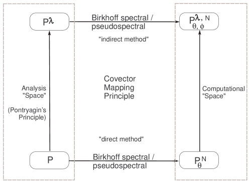
Figure 3: Schematic for the CMP illustrating how discretization commutes with dualization for Birkhoff methods with $\theta,\phi\in\left\{a,b,a^{*},b^{*}\right\}$; figure adapted from [1] and [33].

Once a valid choice of $\pi^{N}$ is made, then a selection of a particular covector mapping theorem can be extracted out of Fig. 3 to construct a fast spectral algorithm[30, 33, 31, 34, 43] that is customized to a particular Birkhoff implementation. Such implementation details are described in part II of this paper[44].

6 Conclusions

Although pseudospectral (PS) theory based on Lagrange interpolants (i.e., PS theory based on differentiation matrices) are already used in mission design and flight operations, its implementation is steeped in various layers of sophistication that manage the growth of condition numbers and round-off errors. It has long been known that the source of these challenges is indeed the starting point; i.e., the use of Lagrange interpolants. Lagrange interpolants also form the basis of Runge-Kutta methods, albeit in their low-order forms. In choosing an altogether new starting point, the Birkhoff theory attacks the problem right at the source. This paper shows that the recently proposed universal Birkhoff interpolant may indeed be used as a new starting point for trajectory optimization. The new direction motivates and integrates many number of disparate concepts in applied mathematics: Birkhoff interpolants, projections in function spaces, spectral (Galerkin) and pseudospectral approximation theories, Pontryagin’s principle, Karush-Kuhn-Tucker theorem, weighted inner-products in finite-dimensional spaces and the covector mapping principle. Despite using a broad swath of results across the mathematical spectrum, a covector mapping theorem can be stated quite simply in terms of its founding principle: a proper discretization can be commuted with dualization. Consequently, many elements of the previously-developed fast spectral algorithm can be easily adapted to the new framework. The net result is that a candidate Birkhoff solution obtained by a “direct method” can be readily verified and validated by using its equivalency with an “indirect method.” More importantly, the equivalences between direct/indirect as well as spectral/pseudospectral methods provide additional avenues for algorithmic acceleration. Combined with the isolation of the Birkhoff-specific computations to a well-conditioned linear system, a Birkhoff-theoretic method is poised to generate fast and accurate solutions to nonlinear trajectory optimization problems.

References

• [1] I. M. Ross, A Primer on Pontryagin’s Principle in Optimal Control, Second Edition, Collegiate Publishers, San Francisco, CA, 2015.
• [2] J. M. Longuski, J. J. Guzmán and J. E. Prussing, Optimal Control with Aerospace Applications, Springer, New York, N.Y., 2014.
• [3] B. A. Conway, “A Survey of Methods Available for the Numerical Optimization of Continuous Dynamic Systems,” Journal of Optimization Theory and Applications, Vol. 152, 2012, pp. 271–306.
• [4] I. M. Ross and F. Fahroo, “A Perspective on Methods for Trajectory Optimization,” AIAA/AAS Astrodynamics Specialist Conference and Exhibit, 5-8 August, 2002, Monterey, CA. AIAA 2002-4727. https://doi.org/10.2514/6.2002-4727.
• [5] Lu, P., “Entry Guidance: A Unified Method,” Journal of Guidance, Control, and Dynamics, Vol. 37, No.3, 2014, pp. 713–728.
• [6] I. M. Ross, P. Sekhavat, A. Fleming and Q. Gong, Q., “Optimal Feedback Control: Foundations, Examples and Experimental Results for a New Approach,” Journal of Guidance, Control, and Dynamics, Vol. 31, No.2, Mar-Apr 2008, pp. 307-321.
• [7] F. Najson, K. D. Mease, “Computationally Inexpensive Guidance Algorithm for Fuel-Efficient Terminal Descent,” Journal of Guidance, Control, and Dynamics, Vol. 29, No.4, 2006, pp. 955-964.
• [8] Bryson, A. E., and Ho, Y.-C., Applied Optimal Control, Hemisphere, New York, 1975 (Revised Printing; original publication, 1969).
• [9] F. Clarke, Functional Analysis, Calculus of Variations and Optimal Control, Springer-Verlag, London, 2013.
• [10] R. B. Vinter, Optimal Control, Birkhäuser, Boston, MA, 2000.
• [11] I. M. Ross, Q. Gong, F. Fahroo and W. Kang, “Practical stabilization through real-time optimal control,” Proceedings of the 2006 American Control Conference, Inst. of Electrical and Electronics Engineers, Piscataway, NJ, June 2006, pp. 14–16.
• [12] Lu, P., “What is Guidance,” Journal of Guidance, Control, and Dynamics, Vol. 44, No.7, July 2021, pp. 1237–1238.
• [13] J. L. Goodman, “Roland Jaggers and the Development of Space Shuttle Powered Explicit Guidance (PEG),” AIAA SciTech Forum Virtual Event, January 11-15 & 19-21, 2021.
• [14] Lu, P., “Propellant-Optimal Powered Descent Guidance,” Journal of Guidance, Control, and Dynamics, Vol. 41, No.4, Mar-Apr 2018, pp. 813–826.
• [15] K. P. Bollino, I. M. Ross and D. Doman, “Optimal nonlinear feedback guidance for reentry vehicles,” AIAA Guidance, Navigation, and Control Conference and Exhibit, Keystone, CO, AIAA-2006-6074, 2006.
• [16] K. P. Bollino and I. M. Ross, “A pseudospectral feedback method for real-time optimal guidance of reentry vehicles,” Proc. of the 2007 IEEE American Control Conference, New York, NY, Jul 2007.
• [17] L.R. Lewis and I.M. Ross, “A pseudospectral method for real-time motion planning and obstacle avoidance” AVT-SCI Joint Symposium on Platform Innovations and System Integration for Unmanned Air, Land and Sea Vehicles, 2007.
• [18] Hurni, M.A., Sekhavat, P., Ross, I.M. (2010). An Info-Centric Trajectory Planner for Unmanned Ground Vehicles. In: Hirsch, M., Pardalos, P., Murphey, R. (eds) Dynamics of Information Systems. Springer Optimization and Its Applications, vol 40. Springer, New York, NY.
• [19] K.P. Bollino and L.R. Lewis, “Collision-free Multi-UAV Optimal Path Planning and Cooperative Control for Tactical Applications,” Proceedings of the AIAA Guidance, Navigation and Control Conference and Exhibit, AIAA 2008-7134, 2008.
• [20] K.P. Bollino and L.R. Lewis, “Optimal path planning and control of tactical unmanned aerial vehicles in urban environments,” Proceedings of the AUVSI’s Unmanned Systems North America Conference, 2007
• [21] K. P. Bollino, L. R. Lewis, P. Sekhavat and I. M. Ross, “Pseudospectral optimal control: a clear road for autonomous intelligent path planning,” AIAA Infotech@Aerospace 2007 Conference and Exhibit, Rohnert Park, CA, AIAA-2007-2831 (2007)
• [22] I. M. Ross and M. Karpenko, “A Review of Pseudospectral Optimal Control: From Theory to Flight,” Annual Reviews in Control, Vol.36, No.2, pp.182–197, 2012.
• [23] W. Kang, I. M. Ross and Q. Gong, “Pseudospectral Optimal Control and its Convergence Theorems,” Analysis and Design of Nonlinear Control Systems, Springer-Verlag, Berlin Heidelberg, 2008, pp. 109–126.
• [24] W. Kang, “Rate of Convergence for a Legendre Pseudospectral Optimal Control of Feedback Linearizable Systems,” Journal of Control Theory and Applications, Vol. 8, No. 4, pp. 391–405, 2010.
• [25] I. M. Ross, Q. Gong and P. Sekhavat, “Low-Thrust, High-Accuracy Trajectory Optimization,” Journal of Guidance, Control and Dynamics, Vol. 30, No. 4, pp. 921–933, 2007.
• [26] I. M. Ross, Q. Gong and P. Sekhavat, “The Bellman Pseudospectral Method,” AIAA/AAS Astrodynamics Specialist Conference and Exhibit, Honolulu, Hawaii, AIAA-2008-6448, August 18-21, 2008.
• [27] H. Yan, Q. Gong, C. Park, I. M. Ross, and C. N. D’Souza, “High Accuracy Trajectory Optimization for a Trans-Earth Lunar Mission,” Journal of Guidance, Control and Dynamics, Vol. 34, No. 4, 2011, pp. 1219-1227.
• [28] R. Baltensperger and M. R. Trummer, “Spectral Differencing with a Twist,” SIAM J. Sci. Comput., 24(5), 14651487, 2003.
• [29] L. N. Trefethen, Spectral Methods in MATLAB, SIAM, Philadelphia, PA, 2000.
• [30] Q. Gong, F. Fahroo and I. M. Ross, “Spectral Algorithm for Pseudospectral Methods in Optimal Control,” Journal of Guidance, Control, and Dynamics, vol. 31 no. 3, pp. 460-471, 2008.
• [31] I. M. Ross and Q. Gong, “Guess-Free Trajectory Optimization,” AIAA/AAS Astrodynamics Specialist Conference and Exhibit, 18–21 August 2008, Honolulu, Hawaii, AIAA 2008-6273.
• [32] I. M. Ross, “An Optimal Control Theory for Nonlinear Optimization,” Journal of Computational and Applied Mathematics, Vol. 354, July 2019, 39–51.
• [33] I. M. Ross, “Enhancements to the DIDO Optimal Control Toolbox,” arXiv preprint, arXiv:2004.13112, 2020, https://arxiv.org/abs/2004.13112
• [34] N. Koeppen, I. M. Ross, L. C. Wilcox and R. J. Proulx, “Fast Mesh Refinement in Pseudospectral Optimal Control,” Journal of Guidance, Control, and Dynamics, vol. 42 no. 4, pp. 711-722, 2018.
• [35] J. S. Hesthaven, “Integration Preconditioning Of Pseudospectral Operators. I. Basic Linear Operators,” SIAM Journal of Numerical Analysis, Vol. 35, No. 4, pp. 1571-1593, 1998.
• [36] E. M. E. Elbarbary, “Integration Preconditioning Matrix for Ultraspherical Pseudospectral Operators,” SIAM Journal of Scientific Computaton, Vol. 28, No. 3, pp. 1186-1201, 2006.
• [37] L.-L Wang, M. D. Samson and X. Zhao, “A Well-Conditioned Collocation Method Using a Pseudospectral Integration Matrix,” SIAM Journal of Scientific Computaton, Vol. 36, No. 3, pp. A907-A929, 2014.
• [38] B. Fornberg, A Practical Guide to Pseudospectral Methods. Cambridge University Press Cambridge, 1996.
• [39] J. Boyd, Chebyshev and Fourier Spectral Methods, Dover Publications, Inc., Minola, New York, 2001.
• [40] G. G. Lorentz and K. L. Zeller, “Birkhoff Interpolation,” SIAM Journal of Numerical Analysis, Vol. 8, No. 1, pp. 43-48, 1971.
• [41] I. J. Schoenberg, “On Hermite-Birkhoff Interpolation,” Journal of Mathematical Analysis and Applications, Vol. 16, No. 3, pp. 538-543, 1966.
• [42] I. M. Ross, R. J. Proulx, C. F. Borges, “A Universal Birkhoff Pseudospectral Method for Solving Boundary Value Problems,” Applied Mathematics and Computation, Vol. 454, 128101, 2023.
• [43] I. M. Ross and R. J. Proulx, “Further Results on Fast Birkhoff Pseudospectral Optimal Control Programming,” Journal of Guidance, Control, and Dynamics, vol. 42 no. 9, pp. 2086–2092, 2019.
• [44] R. J. Proulx and I. M. Ross, “Implementations of the Universal Birkhoff Theory for Fast Trajectory Optimization,” arXiv preprint, arXiv:2308.01450, 2023. https://arxiv.org/pdf/2308.01450.pdf.
• [45] I. M. Ross, A Roadmap for Optimal Control: The Right Way to Commute, Annals of the New York Academy of Sciences, 1065/1, 2005, 210–231.
• [46] Q. Gong, I. M. Ross, W. Kang and F. Fahroo, “On the Pseudospectral Covector Mapping Theorem for Nonlinear Optimal Control,” Proceedings of the 45th IEEE Conference on Decision and Control, 2006, pp. 2679-2686, doi: 10.1109/CDC.2006.377729.
• [47] I. M. Ross, Q. Gong, M. Karpenko and R. J. Proulx, “Scaling and Balancing for High-Performance Computation of Optimal Controls,” Journal of Guidance, Control and Dynamics, Vol. 41, No. 10, 2018, pp. 2086–2097.
• [48] von Stryk, O., Bulirsch, R., “Direct and indirect methods for trajectory optimization,” Annals of Opererations Research, 37, 1992, pp. 357–373.
• [49] Cots, O., Gergaud, J., Goubinat, D., “Direct and indirect methods in optimal control with state constraints and the climbing trajectory of an aircraft,” Optimal Control Applications and Methods, Wiley, 2018, 39, pp. 281–301.
• [50] Q. Gong, W. Kang and I. M. Ross, “A Pseudospectral Method for the Optimal Control of Constrained Feedback Linearizable Systems,” IEEE Transactions on Automatic Control, Vol. 51, No. 7, July 2006, pp. 1115-1129.
• [51] I. Bogaert, Iteration-Free Computation of Gauss–Legendre Quadrature Nodes and Weights, SIAM J. Sci. Comput., 36/3 (2014), A1008-A1026.
• [52] Olver, S., Slevinsky, R., and Townsend, A., “Fast algorithms using orthogonal polynomials,” Acta Numerica, 29, 2021, pp. 573-699.
• [53] Gil, A., Segura, J. and Temme, N.M., “Fast, reliable and unrestricted iterative computation of Gauss-Hermite and Gauss-Laguerre quadratures,” Numerische Mathematik, 143, 2019, pp. 649–682.
• [54] N. Hale, A. Townsend, Fast and Accurate Computation of Gauss–Legendre and Gauss–Jacobi Quadrature Nodes and Weights, SIAM J. Sci. Comput., 35/2 (2013), A652-A674.
• [55] Q. Gong, I. M. Ross and F. Fahroo, “Pseudospectral Optimal Control On Arbitrary Grids,” AAS Astrodynamics Specialist Conference, AAS-09-405, 2009.
• [56] Q. Gong, I. M. Ross and F. Fahroo, “Spectral and Pseudospectral Optimal Control Over Arbitrary Grids,” Journal of Optimization Theory and Applications, vol. 169, no. 3, pp. 759-783, 2016.
• [57] I. H. Sloan, “Nonpolynomial Interpolation,” J. Approx. Theory, 39, 1983, pp. 97–117.
• [58] F. Fahroo and I. M. Ross, “Pseudospectral Methods for Infinite-Horizon Nonlinear Optimal Control Problems,” Proceedings of the AIAA Guidance, Navigation and Control Conference, San Francisco, CA, August 15-18, 2005.
• [59] F. Fahroo and I. M. Ross, “Pseudospectral Methods for Infinite-Horizon Optimal Control Problems,” Journal of Guidance, Control and Dynamics, Vol. 31, No. 4, pp. 927–936, 2008.
• [60] F. Fahroo and I. M. Ross, “Advances in Pseudospectral Methods for Optimal Control,” AIAA Guidance, Navigation, and Control Conference, AIAA Paper 2008-7309, Honolulu, Hawaii, August 2008.
• [61] I. M. Ross and F. Fahroo, “Pseudospectral Knotting Methods for Solving Optimal Control Problems,” Journal of Guidance, Control and Dynamics, Vol. 27, No. 3, pp. 397-405, 2004.
• [62] I. M. Ross and F. Fahroo, “Discrete Verification of Necessary Conditions for Switched Nonlinear Optimal Control Systems,” Proceedings of the American Control Conference, June 2004, Boston, MA.
• [63] Ross, I. M., D’Souza, C. N., “Hybrid Optimal Control Framework for Mission Planning,” Journal of Guidance, Control and Dynamics, Vol. 28, No. 4, pp. 686–697, 2005.
• [64] J. Cullum, “Finite-dimensional approximations of state constrainted continuous optimal problems,” SIAM J. Control, vol. 10, pp. 649–670, 1972.
• [65] H. Halkin, “A Maximum Principle of the Pontryagin Type for Systems Described by Nonlinear Difference Equations,” SIAM Journal of Control, Vol. 4, No. 1, 1966, pp. 90–111.
• [66] B. S. Mordukhovich and I. Shvartsman, “The Approximate Maximum Principle in Constrained Optimal Control,” SIAM Journal of Control and Optimization, Vol. 43, No. 3, 2004, pp. 1037–1062.
• [67] I. M. Ross, “A Historical Introduction to the Covector Mapping Principle,” Advances in the Astronautical Sciences, Vol. 123, Univelt, San Diego, CA, 2006, pp. 1257–1278.
• [68] E. Polak, Optimization: Algorithms and Consistent Approximations, Heidelberg, Germany: Springer-Verlag, 1997.
• [69] P. E. Gill, W. Murray and M. H. Wright, Practical Optimization, Academic Press, London, 1981.