Cross-phase modulation in the two dimensional spectroscopy

Abstract

Developing from the transient absorption (TA) spectroscopy, the two dimensional (2D) spectroscopy with pump-probe geometry has emerged as a versatile approach for alleviating the difficulty on implementing the 2D spectroscopy with other geometries. However, the presence of cross-phase modulation (XPM) in TA spectroscopy introduces significant spectral distortions, particularly when the pump and probe pulses overlap. We demonstrate that this phenomenon is extended to the 2D spectroscopy with pump-probe geometry and the XPM is induced by the interference of the two pump pulse. We present the oscillatory behavior of XPM in the 2D spectrum and its displacement with respect to the waiting time delay through both experimental measurements and numerical simulations. Additionally, we explore the influence of probe pulse chirp on XPM and discover that by compressing the chirp, the impact of XPM on the desired signal can be reduced.

I Introduction

Two dimensional (2D) spectroscopy [1, 2, 3, 4] is a powerful tool with growing attention for studying the couplings and dynamics of systems in both condensed [5, 6, 7, 8] and gaseous phases [9, 10, 11, 12]. Among the various 2D spectroscopy beam geometries [13, 7, 8], the pump-probe geometry [13, 14, 15] developed from the transient absorption (TA) spectroscopy [16, 17, 18, 19, 20] has emerged as a widely adopted approach due to its ease of implementation. In this technique, the pump beam is typically modulated by a pulse shaper [15, 14, 21] which is utilized to generate two identical pump pulses with interval $\tau$ and to compensate for the chirp of the pump pulses [22]. As for the probe arm, the chirp of the probe pulse is often compressed with an extra compressor [23] or even left uncompressed, especially when the super-continuum is applied for probe [15, 24]. Similar to TA spectroscopy, the chirp of the probe pulse would introduce distortions [25, 19, 26] to the spectrum in the 2D case [5, 27, 28]. This occurs because various frequency components of the probe pulse reach the investigated sample at different times [29]. Taking inspiration from the chirp correction scheme used in TA spectroscopy [25, 19, 26], it has been proposed that these distortions in the 2D spectroscopy could be post-corrected [27, 28] by characterizing the chirp of the probe pulse.

Despite the distortion caused by the chirp of the probe pulse, there is another significant artifact induced by the intense pump pulse in the TA spectroscopy known as the cross-phase modulation (XPM) [29, 30, 31, 32, 33]. XPM universally exists in the TA spectroscopy when the pump and probe pulses overlap temporally at the sample, particularly in the system of condensed phase. Moreover, it get stronger as the chirp of the probe pulse increases [29]. As an extension of the TA spectroscopy, the 2D spectroscopy with pump-probe geometry also gets affected by the XPM [34] especially when dynamics within several tens of femtoseconds is investigated. However, a comprehensive theoretical understanding of the XPM in the 2D spectroscopy with pump-probe geometry and its response to variations in the chirp of the probe pulse remain elusive.

In this paper, we present a theoretical derivation of the XPM in the 2D spectroscopy with pump-probe geometry. Our results demonstrate that XPM manifests itself at the central frequency of the pump pulse on the excitation axis and at the central frequency of the probe pulse on the detection axis. Additionally, we observe oscillations and shifts of the XPM along the detection axis, which are supported by experimental data using a sapphire window as the sample and by our numerical simulations. Furthermore, we investigate the effect of probe pulse chirp on the behavior of XPM through the experiments and simulations. We demonstrated that by reducing the chirp of the probe pulse, the influence of XPM on the desired signal is mitigated.

II theory

II.1 General two dimensional spectroscopy

In typical two dimensional spectroscopy experiments, the third-order optical response [1, 2] of a sample is represented by the induced third-order polarization as

$$P^{(3)}\left(t\right)=\int_{0}^{\infty}dt_{3}\int_{0}^{\infty}dt_{2}\int_{0}^{\infty}dt_{1}R^{(3)}\left(t_{1},t_{2},t_{3}\right)E\left(t-t_{3}\right)E\left(t-t_{3}-t_{2}\right)E\left(t-t_{3}-t_{2}-t_{1}\right).$$ (1)

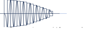
Figure 1: Typical pulse sequence of the two dimensional spectroscopy, where three pulses arrive at the sample at time $t=0$, $t=\tau$, and $t=\tau+T$ sequentially.

where $R^{(3)}\left(t_{1},t_{2},t_{3}\right)$ is the third-order response function of the sample and $E\left(t\right)$ is the external electric field. As Fig. 1 shows, the external field typically consists of three pulses arriving sequentially at time $t=0$, $t=\tau$, and $t=\tau+T$ [21, 35, 5, 36] for 2D setup. As a result, both the external electric field and the induced third-order polarization are functions of $\tau$, $T$ and $t$. Specifically, we denote the induced third-order polarization as $P^{(3)}\left(\tau,T,t\right)$, and the electric field as

$$E\left(\tau,T,t\right)=E_{1}\left(t\right)+E_{2}\left(\tau,t\right)+E_{3}\left(\tau,T,t\right)+\mathrm{c.c.},$$ (2)

$$E_{1}\left(t\right)=A_{1}\left(t\right)\exp\left\{i\left(\vec{k}_{1}\cdot\vec{r}-\Omega_{1}t+\phi_{1}\right)\right\},$$ (3)

$$E_{2}\left(\tau,t\right)=A_{2}\left(t-\tau\right)\exp\left\{i\left[\vec{k}_{2}\cdot\vec{r}-\Omega_{2}\left(t-\tau\right)+\phi_{2}\right]\right\},$$ (4)

$$E_{3}\left(\tau,T,t\right)=A_{3}\left(t-\tau-T\right)\exp\left\{i\left[\vec{k}_{3}\cdot\vec{r}-\Omega_{3}\left(t-\tau-T\right)+\phi_{3}\right]\right\}.$$ (5)

where $A_{m}$, $\vec{k}_{m}$, $\Omega_{m}$, and $\phi_{m}$ $(m=1,2,3)$ are respectively the envelopes, wave vectors, central frequencies, and initial phases of the pulses, and $\vec{r}$ is the spatial location of the sample molecule. The possible dispersion of the pulses is encoded into the envelopes. For a transparent sample with length $L$, the induced polarization yields signal [1] field

$$E_{s}\left(\tau,T,t\right)=\frac{2\pi i}{n}\frac{\Omega_{s}L}{c}P^{(3)}\left(\tau,T,t\right)=i\eta\Omega_{s}P^{(3)}\left(\tau,T,t\right),$$ (6)

along several phase matching directions $\vec{k}_{s}=\pm\vec{k}_{\alpha}\pm\vec{k}_{\beta}\pm\vec{k}_{\gamma}$ ($\alpha,\beta,\gamma=1,2,3$), where $\eta=2\pi L/cn$, $n$ is the linear refractive index of the sample, $c$ is the speed of light, and $\Omega_{s}$ is the central frequency of the signal field.

In general, the two dimensional (2D) spectrum $E_{s}\left(\omega_{\tau},T,\omega_{t}\right)$ is obtained by Fourier transforming $E_{s}\left(\tau,T,t\right)$ with respect to $\tau$ and $t$. In some cases, the time domain signal $E_{s}\left(\tau,T,t\right)$ is collected by scanning both $\tau$ and $t$ [9, 10, 7, 8]. Alternatively, it is popular to heterodynely detect [1, 35, 5] the frequency domain signal $E_{s}\left(\tau,T,\omega_{t}\right)$ via a spectrometer and with a local oscillator $E_{\mathrm{LO}}\left(t\right)$. In this technique, the differential optical signal $S\left(\tau,T,\omega_{t}\right)$ is obtained as

$$S\left(\tau,T,\omega_{t}\right)=\ln\frac{I_{s}\left(\tau,T,\omega_{t}\right)}{I_{\mathrm{LO}}\left(\omega_{t}\right)}\simeq\frac{I_{s}\left(\tau,T,\omega_{t}\right)}{I_{\mathrm{LO}}\left(\omega_{t}\right)}-1\simeq\frac{2\mathrm{Re}\left[E_{s}\left(\tau,T,\omega_{t}\right)E_{\mathrm{LO}}^{*}\left(\omega_{t}\right)\right]}{\left|E_{\mathrm{LO}}\left(\omega_{t}\right)\right|^{2}}=2\mathrm{Re}\left[\frac{E_{s}\left(\tau,T,\omega_{t}\right)}{E_{\mathrm{LO}}\left(\omega_{t}\right)}\right],$$ (7)

where $I_{\mathrm{LO}}\left(\omega_{t}\right)=\left|E_{\mathrm{LO}}\left(\omega_{t}\right)\right|^{2}$ and $I_{s}\left(\tau,T,\omega_{t}\right)=\left|E_{s}\left(\tau,T,\omega_{t}\right)+E_{\mathrm{LO}}\left(\omega_{t}\right)\right|^{2}\simeq 2\mathrm{Re}\left[E_{s}\left(\tau,T,\omega_{t}\right)E_{\mathrm{LO}}^{*}\left(\omega_{t}\right)\right]+\left|E_{\mathrm{LO}}\left(\omega_{t}\right)\right|^{2}$, because the signal field is usually much weaker than the local oscillator, i.e., $\left|E_{s}\left(\tau,T,\omega_{t}\right)\right|\ll\left|E_{\mathrm{LO}}\left(\omega_{t}\right)\right|$. The 2D spectrum $S\left(\omega_{\tau},T,\omega_{t}\right)$ is then obtained by scanning and Fourier transforming with respect to only $\tau$,

$$S\left(\omega_{\tau},T,\omega_{t}\right)=\mathcal{F}\left[S\left(\tau,T,\omega_{t}\right)\right].$$ (8)

II.2 Two dimensional spectroscopy with pump-probe geometry

There are several experimental beam geometries in the 2D spectroscopy based on the direction arrangement of the three pulses, such as collinear geometry [10, 7, 8] and non-collinear BOXCARS geometry [5, 35]. Besides, there is a partially collinear geometry known as the pump-probe geometry [13, 14, 15] where the first two pulses are collinear $\vec{k}_{1}=\vec{k}_{2}$ and the third pulse serves also as the local oscillator. Such a beam geometry is identical with the TA (pump-probe) spectroscopy geometry [16, 17, 18, 19, 20]. The first two pulses are often denoted as the pump pulses and the third pulse as the probe pulse. The pump-probe geometry eases the difficulty of experimentally implementing the 2D spectroscopy compared with the other geometries, because the heterodyne detection is naturally satisfied by measuring the spectrum of probe pulse, i.e., $\vec{k}_{s}=\vec{k}_{3}$. However, signal fields that are spatially separated in the BOXCARS geometry may get mixed [14, 23] in the pump-probe geometry. Specifically, signal fields $E_{\alpha^{\prime},-\alpha^{\prime},3}\left(\tau,T,\omega_{t}\right)$, $E_{1,-2,3}\left(\tau,T,\omega_{t}\right)$, and $E_{-1,2,3}\left(\tau,T,\omega_{t}\right)$ are all emit along $\vec{k}_{3}$ in the pump-probe geometry. Here, $\alpha^{\prime}=\pm 1,\pm 2,\pm 3$ and the subscripts of the signal field $E_{\alpha,\beta,\gamma}$ denote that the signal is induced by incident fields $E_{\alpha}$, $E_{\beta}$, and $E_{\gamma}$ (or their conjugation if the corresponding subscripts are negative). Among all these mixed signals, $E_{-1,2,3}\left(\tau,T,\omega_{t}\right)$ and $E_{1,-2,3}\left(\tau,T,\omega_{t}\right)$ are typically required for the study of single-quantum coherence in the excitation time $\tau$. These two signals are often denoted as the rephasing and non-rephasing signal [1, 5], respectively.

To sort out only $E_{-1,2,3}\left(\tau,T,\omega_{t}\right)$ and $E_{1,-2,3}\left(\tau,T,\omega_{t}\right)$ in the total signal field, the technique of phase cycling [14, 23, 11] is applied. According to the discussion in Sec. II.1, the signal field $E_{s}\left(\tau,T,\omega_{t}\right)$ from the sample depends on the initial phase $\phi_{\alpha}$ of the incident fields. However, in the 2D spectroscopy with pump-probe geometry, the phase of the third pulse $\phi_{3}$ is eliminated because the third pulse serves as the local oscillator in the heterodyne detection [14]. Thus, we denote the phase-depend signal field as $E_{s}\left(\tau,T,\omega_{t};\phi_{1},\phi_{2}\right)$ and its components

$$E_{\alpha,\beta,3}\left(\tau,T,\omega_{t};\phi_{1},\phi_{2}\right)=E_{\alpha,\beta,3}\left(\tau,T,\omega_{t}\right)\exp\left\{i\left[\mathrm{sgn}\left(\alpha\right)\times\phi_{\left|\alpha\right|}+\mathrm{sgn}\left(\beta\right)\times\phi_{\left|\beta\right|}\right]\right\},$$ (9)

where $\alpha,\beta=\pm 1,\pm 2,\pm 3$, $\mathrm{sgn}\left(x\right)=x/\left|x\right|$ is the sign function, and the phase free term $E_{\alpha,\beta,3}\left(\tau,T,\omega_{t}\right)$ denotes the signal field with initial phases $\phi_{1},\phi_{2}=0$ of the first two pulses. By conducting two experiments with phase arrangements a) $\phi_{1}=\pi$ and $\phi_{2}=0$; b) $\phi_{1}=\pi$ and $\phi_{2}=\pi$, the phase cycled signal is given as

$$S_{\mathrm{cyc}}\left(\tau,T,\omega_{t}\right)=\ln\frac{I\left(\tau,T,\omega_{t};\pi,0\right)}{I\left(\tau,T,\omega_{t};\pi,\pi\right)}\simeq\frac{I\left(\tau,T,\omega_{t};\pi,0\right)}{I\left(\tau,T,\omega_{t};\pi,\pi\right)}-1\simeq\frac{I\left(\tau,T,\omega_{t};\pi,0\right)-I\left(\tau,T,\omega_{t};\pi,\pi\right)}{I\left(\tau,T,\omega_{t};\pi,\pi\right)},$$ (10)

with

$$I\left(\tau,T,\omega_{t};\phi_{1},\phi_{2}\right)=\left|E_{s}\left(\tau,T,\omega_{t};\phi_{1},\phi_{2}\right)+E_{3}(\omega_{t})\right|^{2}\simeq\left|E_{3}(\omega_{t})\right|^{2}+2\mathrm{Re}\left[E_{s}\left(\tau,T,\omega_{t};\phi_{1},\phi_{2}\right)E_{3}^{*}(\omega_{t})\right],$$ (11)

$I_{3}\left(\omega_{t}\right)=\left|E_{3}(\omega_{t})\right|^{2}$, and $\left|E_{s}\left(\tau,T,\omega_{t};\phi_{1},\phi_{2}\right)\right|\ll\left|E_{3}(\omega_{t})\right|$. Then, the phase cycled signal is expressed as

$$S_{\mathrm{cyc}}\left(\tau,T,\omega_{t}\right)=2\mathrm{Re}\left[\frac{E_{s}\left(\tau,T,\omega_{t};\pi,0\right)-E_{s}\left(\tau,T,\omega_{t};\pi,\pi\right)}{E_{3}\left(\omega_{t}\right)}\right],$$ (12)

which includes only the signals $E_{-1,2,3}$ and $E_{1,-2,3}$, while the parts $E_{\alpha^{\prime},-\alpha^{\prime},3}$ are eliminated because they are not affected by the initial phases of the pump pulses. The 2D spectrum $S_{\mathrm{cyc}}\left(\omega_{\tau},T,\omega_{t}\right)$ is obtained by firstly scanning $\tau$ to collect a series of $S_{\mathrm{cyc}}\left(\tau,T,\omega_{t}\right)$ and then Fourier transforming $S_{\mathrm{cyc}}\left(\tau,T,\omega_{t}\right)$ with respect to $\tau$. The rephasing and non-rephasing parts can further be separated with additional phase cycling [23].

II.3 Cross-phase modulation in the two dimensional spectroscopy with pump-probe geometry

In most spectroscopy experiments, the frequencies of the incident electric fields are typically chosen to resonate with (or nearly resonate with) one of the transition frequencies of the investigated sample, thereby changing the absorption rate [1, 2] (imaginary part of the electric susceptibility) of the sample accordingly. However, in liquid sample where the solution (i.e., the investigated sample) is dissolved in a specific solvent, the electric fields also induce the non-resonant electronic response (ER) of the solvent, altering the refractive index [37, 34] (real part of the electric susceptibility) of the solvent through Kerr effect. The ER is approximately instantaneous [37, 38] (with a time scale of $0.1\sim 1\>\mathrm{fs}$) compared with the resonant response of the solution and the duration of the incident pulses (with a time scale of $10\sim 100\>\mathrm{fs}$). Therefore, the response function [37, 29, 34] is approximately written as

$$R_{\mathrm{ER}}^{(3)}\left(t_{1},t_{2},t_{3}\right)=\sigma_{e}\delta\left(t_{1}\right)\delta\left(t_{2}\right)\delta\left(t_{3}\right).$$ (13)

Substituting Eq. (13) into Eq. (1), the induced polarization of the electronic response is given as $P^{\mathrm{ER}}\left(\tau,T,t\right)=\sigma_{e}\left[E\left(\tau,T,t\right)\right]^{3}$, and the corresponding signal field is

$$E_{s}^{\mathrm{ER}}\left(\tau,T,t\right)=i\sigma_{e}\eta\Omega_{s}\left[E\left(\tau,T,t\right)\right]^{3}.$$ (14)

Among all the heterodynely detected signal components in the 2D spectroscopy with pump-probe geometry, $E_{3,-3,3}^{\mathrm{ER}}\left(\tau,T,t\right)$ and $E_{-3,3,3}^{\mathrm{ER}}\left(\tau,T,t\right)$ are treated as the self-phase modulation (SPM) [39] which describes the spectral and temporal modulation of the probe pulse induced by itself. The other components are cross-phase modulation (XPM) [29, 30, 31, 32, 33], describing the spectral and temporal modulation of the probe pulse induced by the first pump pulse only [$E_{1,-1,3}^{\mathrm{ER}}\left(\tau,T,t\right)$ and $E_{-1,1,3}^{\mathrm{ER}}\left(\tau,T,t\right)$], the second pump pulse only [$E_{2,-2,3}^{\mathrm{ER}}\left(\tau,T,t\right)$ and $E_{-2,2,3}^{\mathrm{ER}}\left(\tau,T,t\right)$], or the interference of the two pump pulses [$E_{-1,2,3}^{\mathrm{ER}}\left(\tau,T,t\right)$ and $E_{1,-2,3}^{\mathrm{ER}}\left(\tau,T,t\right)$] where

$$E_{-1,2,3}^{\mathrm{ER}}\left(\tau,T,t\right) =i\sigma_{e}\eta\Omega_{s}E_{1}^{*}\left(t\right)E_{2}\left(t-\tau\right)E_{3}\left(t-\tau-T\right),$$ (15)

$$E_{1,-2,3}^{\mathrm{ER}}\left(\tau,T,t\right) =i\sigma_{e}\eta\Omega_{s}E_{1}\left(t\right)E_{2}^{*}\left(t-\tau\right)E_{3}\left(t-\tau-T\right).$$ (16)

Via the phase cycling technique [14, 23, 11] described in Sec. II.2, all the modulations of the probe pulse induced by a single pulse $E_{\alpha^{\prime},-\alpha^{\prime},3}^{\mathrm{ER}}$ are eliminated. Whereas, the modulations from the interference of the two pump pulses remain,

$$S_{\mathrm{XPM}}\left(\tau,T,\omega_{t}\right)=-4\mathrm{Re}\left[\frac{E_{-1,2,3}^{\mathrm{ER}}\left(\tau,T,\omega_{t}\right)+E_{1,-2,3}^{\mathrm{ER}}\left(\tau,T,\omega_{t}\right)}{E_{3}\left(\omega_{t}\right)}\right],$$ (17)

where $E_{-1,2,3}^{\mathrm{ER}}\left(\tau,T,\omega_{t}\right)$ and $E_{1,-2,3}^{\mathrm{ER}}\left(\tau,T,\omega_{t}\right)$ are XPM signal fields when the initial phases of the two pump pulses $\phi_{1},\phi_{2}=0$.

To give more explicit expressions of the XPM signal $S_{\mathrm{XPM}}\left(\tau,T,\omega_{t}\right)$, we assume that the two pump pulses are Fourier transform limited Gaussian pulses without chirp, i.e.,

$$E_{1}\left(t\right)=a_{1}\exp\left\{-\frac{t^{2}}{2\tau_{1}^{2}}\right\}\exp\left\{-i\Omega_{1}t\right\},$$ (18)

$$E_{2}\left(\tau,t\right)=a_{2}\exp\left\{-\frac{\left(t-\tau\right)^{2}}{2\tau_{2}^{2}}\right\}\exp\left\{-i\Omega_{2}\left(t-\tau\right)\right\},$$ (19)

and the probe pulse is a Gaussian pulse with linear chirp [29, 28]

$$E_{3}\left(\tau,T,t\right)=a_{3}\exp\left\{-\frac{\left(t-\tau-T\right)^{2}}{2\tau_{3}^{2}}\right\}\exp\left\{-i\left[\Omega_{3}\left(t-\tau-T\right)+\beta_{3}\left(t-\tau-T\right)^{2}\right]\right\},$$ (20)

where $a_{\alpha}$ and $\tau_{\alpha}$ are the amplitude and duration of pulse $E_{\alpha}$, and $\beta_{3}$ is the chirp rate of the probe pulse. The spatial phase factors and initial phases are neglected here. We further simplify our model by assuming $a_{1}=a_{2}$, $\tau_{1}=\tau_{2}$, and $\Omega_{1}=\Omega_{2}$, which is accessible with the pulse shaper [15, 14, 21] on the pump arm. With these incident pulses in Eq. (18-20), we obtain the phase cycled XPM signal as

$$S_{\mathrm{XPM}}\left(\tau,T,\omega_{t}\right) =\frac{8}{A^{1/4}}\sigma_{e}\eta\Omega_{3}\tau_{1}\left|a_{1}\right|^{2}\cos\left(\Omega_{1}\tau\right)\exp\left\{-\frac{\tau^{2}}{4\tau_{1}^{2}}\right\}$$ (21)

$$\times\exp\left\{\frac{\left(\tau_{1}^{2}+2\tau_{3,0}^{2}\right)B-4\beta_{gdd}\tau_{3,0}^{2}\left(\Omega_{3}-\omega_{t}\right)t_{d}\left(\omega_{t}\right)}{A}\right\}$$

$$\times\sin\left\{\frac{2\beta_{gdd}B+2\tau_{3,0}^{2}\left(\Omega_{3}-\omega_{t}\right)\left(\tau_{1}^{2}+2\tau_{3,0}^{2}\right)t_{d}\left(\omega_{t}\right)}{A}+\phi\right\},$$

where $A=\left(\tau_{1}^{2}+2\tau_{3,0}^{2}\right)^{2}+4\beta_{gdd}^{2}$, $B=\left[t_{d}\left(\omega_{t}\right)\right]^{2}+\tau_{3,0}^{4}\left(\Omega_{3}-\omega_{t}\right)^{2}$, $t_{d}\left(\omega_{t}\right)=\tau/2+T-\beta_{gdd}\left(\Omega_{3}-\omega_{t}\right)$, and $\phi=\arctan\left[2\beta_{gdd}/\left(\tau_{1}^{2}+2\tau_{3,0}^{2}\right)\right]$. The parameters $\beta_{gdd}$ and $\tau_{3,0}$ are the group delay velocity (GDD) and Fourier limited duration of the probe pulse, respectively. These two parameters are connected to $\tau_{3}$ and $\beta_{3}$ with relation $\tau_{3}^{2}=\left(\tau_{3,0}^{4}+\beta_{gdd}^{2}\right)/\tau_{3,0}^{2}$ and $\beta_{3}=0.5\beta_{gdd}/\left(\tau_{3,0}^{4}+\beta_{gdd}^{2}\right)$ [28].

The cosine term $\cos\left(\Omega_{1}\tau\right)$ and the Gaussian term with variable $\left(\Omega_{3}-\omega_{t}\right)$ in Eq. (21) indicate that the XPM signal on the 2D spectrum covers around $\left(\omega_{\tau}=\Omega_{1},\omega_{t}=\Omega_{3}\right)$, i.e., typically the resonant frequencies of the sample solution. We remark that the XPM signal are oscillating along $\omega_{t}$ govern by the sine term in Eq. (21), and the oscillation will move along $\omega_{t}$ as $T$ changes. We will show such features with experiments and simulations in the following sections.

III Experiment and simulation

III.1 Experimental Setup

Our experimental setup is presented in Fig. 2. Laser pulses (800 nm, 7.15 W, 30.8 fs, at a 1 kHz repetition rate, and horizontally polarized with respect to the table surface) delivered by the Ti:Sapphire amplifier laser system are lead into an optical parametric amplifier (OPA) to produce pulses with desired central wavelength at 680 nm. The laser beam is then lead into a commercial integrated 2D spectroscopy system. Specifically, the laser beam after the OPA is divided by a wedged window into two beams, i.e., the pump and probe beams, and the power of the probe beam is controlled by a half-wave plate before the wedged window. To introduce time delays between the pump and probe pulses, the pump beam is directed into a pulse shaper and a delay stage before hitting the sample. The pulse shaper [15, 14, 21] consists of an acousto-optic modulator (AOM), two parabolic mirrors, and two gratings with 4-f geometry. The AOM, synchronized with our laser system, modulates the first-order diffraction of the pump pulses with customized mask through photoelastic effect. Typically, the mask is designed such that one pump pulse is divided into two identical transform limited pump pulses with interval $\tau$. The time delay $T$ between the probe and the second pump pulse is controlled by the delay stage. The pump and probe beams are aligned in parallel and focused onto the sample using a parabolic mirror. After the sample, the pump beam is blocked by a beam trap, and the probe beam, passing through a Glan-Taylor prism and a lens ($f=300\>\mathrm{mm}$), is lead into a spectrometer with the spectrum detected by a charge coupled device (CCD) camera. The Glan-Taylor prism is used to guarantee that only horizontally polarized component of the probe pulse is measured. Furthermore, a half-wave plate and a polarizer in the pump arm before the sample are utilized to ensure that only horizontally polarized component pump pulses interact with the sample.

In our 2D spectroscopy experiment for detecting the XPM, a sapphire window (3 mm) serves as the sample. Additionally, to study the influence of the GDD of the probe pulse to the XPM on the 2D spectrum, two experiments are conducted. In our first experiment, the probe beam passes freely before the sample, while in the second experiment, an additional sapphire window (SW, 3 mm thick) is placed on probe arm to alter the $\beta_{gdd}$ of the probe pulse.

We remark that the phases of the pump pulses are also controlled by the AOM, making phase cycling available in this system. Moreover, instead of the two-frame cycling $(\phi_{1}=\pi,\phi_{2}=0)$ and $(\phi_{1}=\pi,\phi_{2}=\pi)$ introduced in Sec. II.2, we actually utilize a four-frame cycling [14] $(\phi_{1}=\pi,\phi_{2}=0)$, $(\phi_{1}=\pi,\phi_{2}=\pi)$, $(\phi_{1}=0,\phi_{2}=\pi)$, and $(\phi_{1}=0,\phi_{2}=0)$, which further eliminates the scatter from the pump pulses.

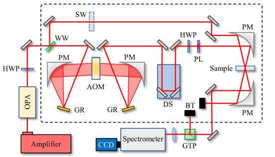
Figure 2: Schematic experimental setup of the 2D spectroscopy with pump-probe geometry in our experiment. Amplifier: Ti:Sapphire amplifier laser system; OPA: optical parametric amplifier; HWP: half-wave plate; WW: wedged window; PM: parabolic mirror; GR: optical grating; AOM: acousto-optic modulator; DS: delay stage; PL: polarizer; SW: sapphire window (3 mm) used to altering the GDD of the probe pulse; BT: beam trap; GTP: Glan-Taylor prism; Spectrometer: spectrometer; CCD: charge coupled device camera. The system enclosed by a dash box is an integrated 2D spectroscopy system. In our 2D spectroscopy experiment for detecting the XPM, a sapphire window (3 mm) serves as the sample.

III.2 Pulse parameters

We presented in this section the parameters of the pulses applied in our experiments. The spectrum of the probe pulse is shown in Fig. 3(a), with the central frequency $\Omega_{3}/2\pi=438.09\>\mathrm{THz}$ and the bandwidth $\sigma_{3,0}/2\pi=11.74\>\mathrm{THz}$ evaluated by the Gaussian fitting of the spectrum. The bandwidth $\sigma_{3,0}$ corresponds to a Fourier limited duration of the probe pulse, $\tau_{3,0}=1/\sigma_{3,0}=13.56\>\mathrm{fs}$. The auto-correlation functions (ACF) of the probe pulses $E_{3}^{e_{1}}$ and $E_{3}^{e_{2}}$ are given in Fig. 3(b) and (c). Here, the superscripts $e_{1}$ and $e_{2}$ are used to denote experiments without and with the additional SW on the probe arm, respectively. The duration of the ACFs are $\tau_{\mathrm{ACF}}^{e_{1}}=47.25\>\mathrm{fs}$ and $\tau_{\mathrm{ACF}}^{e_{2}}=66.50\>\mathrm{fs}$, and the duration of the electric fields are directly given by the ACFs as $\tau_{3}^{e_{1}}=\tau_{\mathrm{ACF}}^{e_{1}}=47.25\>\mathrm{fs}$ and $\tau_{3}^{e_{2}}=\tau_{\mathrm{ACF}}^{e_{2}}=66.50\>\mathrm{fs}$. Such duration of the electric fields corresponds to the typical positive GDDs $\beta_{gdd}^{e_{1}}=613.76\>\mathrm{fs}^{2}$ and $\beta_{gdd}^{e_{2}}=882.79\>\mathrm{fs}^{2}$ according to the relation $\beta_{gdd}^{2}=\tau_{3,0}^{2}\left(\tau_{3}^{2}-\tau_{3,0}^{2}\right)$. The spectrum is collected by the spectrometer and CCD camera, and the ACFs are measured by an auto-correlator.

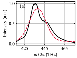
Figure 3: (a) The spectrum and (b, c) the auto-correlation functions (ACFs) of the probe pulses. The black solid lines are experimental results and the red dash lines are Gaussian fittings. The Gaussian fitting in (a) suggests that the probe spectrum centered at $\Omega_{3}/2\pi=438.09\>\mathrm{THz}$ with the bandwidth $\sigma_{3,0}/2\pi=11.74\>\mathrm{THz}$. Such a bandwidth corresponds to a Fourier limited duration $\tau_{3,0}=1/\sigma_{3,0}=13.56\>\mathrm{fs}$ of the probe pulse. The ACFs in (b) and (c) relate to the probe pulses without and with the additional SW, respectively. Via the Gaussian fitting, the duration of the ACFs are $\tau_{\mathrm{ACF}}^{e_{1}}=47.25\>\mathrm{fs}$ for (b) and $\tau_{\mathrm{ACF}}^{e_{2}}=66.50\>\mathrm{fs}$ for (c) corresponding to the duration $\tau_{3}^{e_{1}}=\tau_{\mathrm{ACF}}^{e_{1}}=47.25\>\mathrm{fs}$ and $\tau_{3}^{e_{2}}=\tau_{\mathrm{ACF}}^{e_{2}}=66.50\>\mathrm{fs}$ for the probe pulses.

The parameters of the pump pulses are not measured with the spectrometer, instead we evaluate the parameters of the pump pulses by simulating the 2D correlation spectra of the XPM (referred to as 2DCS-XPM) and Gaussian fitting their projection traces on the axis of $\omega_{\tau}$. Firstly, the central frequencies of the pump pulses are determined by projecting the experimental results of the 2DCS-XPM onto the axis of $\omega_{\tau}$. Then the simulations are conducted by scanning the duration of the pump pulses to obtain the best duration, with which the simulated projection trace fits best with the experiment (See Supplementary for details). The central frequencies and best duration of the pump pulses are $\Omega_{1}^{e_{1}}/2\pi=449.59\>\mathrm{THz}$ and $\tau_{1}^{e_{1}}=48.85\>\mathrm{fs}$ for experiment without the SW and $\Omega_{1}^{e_{2}}/2\pi=449.19\>\mathrm{THz}$ and $\tau_{1}^{e_{2}}=50.48\>\mathrm{fs}$ for experiment with the SW. These parameters are utilized in Sec. III.4 for numerical simulation.

III.3 XPM in 2D spectroscopy experiments

We have measured the 2DCS-XPM using a sapphire window as the sample. The time delay $T$ is scanned from -100 fs to 30 fs with a step size of 10 fs. The results from $T=-20\;\mathrm{fs}$ to $T=20\;\mathrm{fs}$ with 65% contours are shown in Fig. 4, where the spectra in the first row are measured without the SW and those in the second row are measured with the SW on the probe arm.

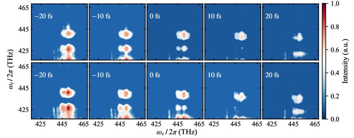
Figure 4: 2D correlation spectra of the XPM by using a sapphire window as the sample with the corresponding $T$ denoted on. The spectra in the first row are measured when the SW is absent on the probe arm. The spectra in the second row are measured with the the SW placed. Those 2D spectra are obtained by Fourier transform the time domain signal $S_{\mathrm{XPM}}\left(\tau,T,\omega_{t}\right)$ with respect to $\tau$ and then taking the absolute value of the transform results. To stress the signal from the background and from the noise, 65% contours are shown here.

In Fig. 4, up to three peaks along $\omega_{t}$ are observable. Those peaks correspond to the oscillation of the $S_{\mathrm{XPM}}\left(\tau,T,\omega_{t}\right)$ introduced by the sine term in Eq. (21). The additional peaks, which are also predicted by the sine term, are not visible here constrained by the signal-to-noise ratio. We remark that the intensities of the 2DCS-XPM presented in Fig. 4 are stronger when $T$ is negative than the positive ones. This discrepancy arises due to the greater likelihood of the probe pulse overlapping with the interference of the two pump pulses under negative $T$ conditions.

Another feature of the 2DCS-XPM is the dynamic shift along $\omega_{t}$ from higher frequency (shorter wavelength) to smaller frequency (longer wavelength) regions as the delay time $T$ increases. We emphasize such a tendency by projecting the 2DCS-XPM onto the axis of $\omega_{t}$, and the instances from $T=-20\;\mathrm{fs}$ to $T=20\;\mathrm{fs}$ are presented in Fig. 5(a) for experiment without the SW and Fig. 5(b) for experiment with the SW. After the projection, one particular peak near $\Omega_{3}$ of the projection traces, e.g., the one enclosed by red square in Fig. 5(a) or blue square in Fig. 5(b), is fitted with the quadratic polynomial to obtain a central frequency of the peak. Fig. 5(c) and (d) illustrates the shifts of the central frequencies as $T$ changes from -100 fs to 30 fs with the red dots (for experiment without the SW) and the blue triangles (for experiment with the SW), respectively. The shifts are nearly linear about $T$ in both experiments and the slopes of the linear fitting lines are $-0.205\>\mathrm{THz}/\mathrm{fs}$ for experiment without the SW and $-0.153\>\mathrm{THz}/\mathrm{fs}$ for experiment with the SW. The slope characterizes the speed of the peak displacement, and thus the result shows that the XPM moves faster when the probe pulse is less chirped.

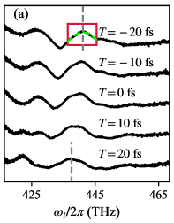
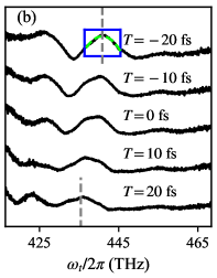
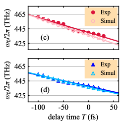
Figure 5: (a, b) Projection traces of the 2DCS-XPM onto the axis of $\omega_{t}$ and (c, d) the dynamic shifts of the XPM along the axis of $\omega_{t}$ as $T$ changes. The traces in (a) and the shifts in (c) correspond to the 2DCS-XPM without the SW and those in (b) and (d) correspond to the 2DCS-XPM with the SW on the probe arm. The displacement of the traces in (a) and (b) are indicated by the gray dash lines, representing the central frequencies of one specific peak, e.g., the one enclosed by red square in (a) or blue square in (b) when $T=-20\;\mathrm{fs}$. The central frequencies are obtained by fitting the peaks using the quadratic polynomial (green dash lines). The shifts of the central frequencies as functions of $T$ are quantified in (c) by the red dots and in (d) by the blue solid triangles. Their corresponding linear fitting lines have slopes of $-0.205\>\mathrm{THz}/\mathrm{fs}$ and $-0.153\>\mathrm{THz}/\mathrm{fs}$, respectively. Additionally, the simulation results are depicted in (c) by the pink circles and in (d) by the light-blue hollow triangles, with the slopes of their linear fitting lines being $-0.231\>\mathrm{THz}/\mathrm{fs}$ and $-0.165\>\mathrm{THz}/\mathrm{fs}$, respectively.

III.4 Simulation

To verify the mechanism of the XPM on the 2D spectroscopy, we simulate the 2DCS-XPM using Eq. (21) and with the pulse parameters in Sec. III.2. The simulation results from $T=-20\;\mathrm{fs}$ to $T=20\;\mathrm{fs}$ with 65% contours are taken as the instances in Fig. 6, where three distinct peaks are observed as in the experimental results in Fig. 4. Also, as in Fig. 4, simulations in the first row in Fig. 6 correspond to experiment without the SW, and those in the second row correspond to experiment with the SW.

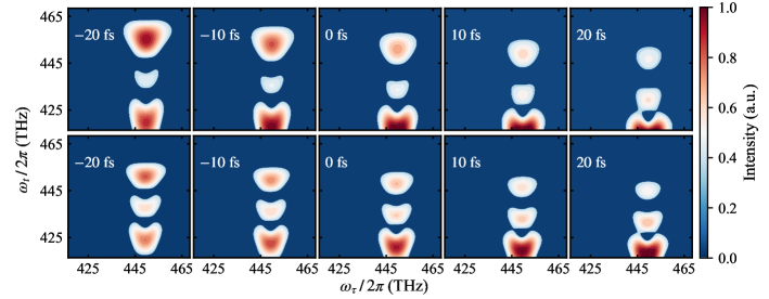
Figure 6: Simulated 2DCS-XPM with the corresponding $T$ denoted on. The spectra in the first row are simulated for the experiment without the SW, and the parameters are $\Omega_{3}/2\pi=438.09\>\mathrm{THz}$, $\beta_{gdd}^{e_{1}}=613.76\>\mathrm{fs}^{2}$ for the probe pulse, and $\Omega_{\tau}^{e_{1}}/2\pi=449.59\>\mathrm{THz}$, $\tau_{1}^{e_{1}}=48.85\>\mathrm{fs}$ for the pump pulses. The spectra in the second row are simulated for the experiment with the SW, and the parameters are $\Omega_{3}/2\pi=438.09\>\mathrm{THz}$, $\beta_{gdd}^{e_{2}}=882.79\>\mathrm{fs}^{2}$ for the probe pulse, and $\Omega_{1}^{e_{2}}/2\pi=449.19\>\mathrm{THz}$, $\tau_{1}^{e_{2}}=50.48\>\mathrm{fs}$ for the pump pulses. 65% contours are shown here.

We also illustrate the dynamic shifts of the XPM on the simulated 2D spectra by projecting them onto the axis of $\omega_{t}$ and then fitting the peak near $\Omega_{3}$ to obtain a central frequency. The shifts of the central frequencies in our simulations are depicted in Fig. 5(c) and (d), alongside the corresponding experimental results. In Fig. 5(c) and (d), the displacements of the simulations (represented by the hollow marks) meet well with the experimental results (represented by the solid marks) for both experiments without and with the SW. The slope of the linear fittings of the simulations are $-0.231\>\mathrm{THz}/\mathrm{fs}$ and $-0.165\>\mathrm{THz}/\mathrm{fs}$, close to the experimental results $-0.205\>\mathrm{THz}/\mathrm{fs}$ and $-0.153\>\mathrm{THz}/\mathrm{fs}$. Both experiments and simulations prove that as the chirp of the probe pulse gets larger, the XPM moves slower with respect to delay time $T$ and will cover the desired signal for a wider range of $T$.

The speed of the XPM displacement as a function of the GDD of the probe pulse $\beta_{gdd}$ is presented in Fig. 7, where the slopes for both positive and negative $\beta_{gdd}$ are simulated (red solid marks) and then fitted (red dash lines) with reciprocal function. Unlike in the positive $\beta_{gdd}$ region where the slope is negative and the XPM moves from higher frequency (shorter wavelength) to smaller frequency (longer wavelength), in the negative $\beta_{gdd}$ region, slope is positive and the XPM moves from smaller frequency (longer wavelength) to larger frequency (shorter wavelength). Whereas, the reciprocal relation between the slope and the $\beta_{gdd}$ retains. Such a reciprocal relation moves the XPM away from the frequency region of interest much faster with respect to $T$ as $\beta_{gdd}$ decreases. Hence, suppressing the chirp of the probe pulse also suppresses the range of $T$ within which the desired signal is affected by the XPM. Moreover, the intensity of the XPM at $T=0\>\mathrm{fs}$ is significantly reduced by suppressing $\beta_{gdd}$, as depicted by the black solid line in Fig. 7. With these two features, one is able to minimize the influence of the XPM on the 2D spectroscopy by suppressing the chirp of the probe pulse.

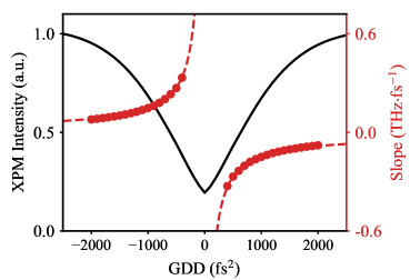
Figure 7: Simulated intensities and moving speed of the XPM on the 2D spectra as functions of the GDD of the probe pulse. In the simulation, the central frequency and the Fourier limited duration of the probe pulse are $\Omega_{3}/2\pi=438.09\>\mathrm{THz}$ and $\tau_{3,0}=13.56\>\mathrm{fs}$, and the central frequency and the Fourier limited duration of the pump pulse are $\Omega_{1}/2\pi=449.46\>\mathrm{THz}$ and $\tau_{1}=50\>\mathrm{fs}$. The maximum intensity of the XPM within the region $\left\{\left(\omega_{\tau},\omega_{t}\right)|444.46\>\mathrm{THz}\leq\omega_{\tau}/2\pi\leq 454.46\>\mathrm{THz},433.09\>\mathrm{THz}\leq\omega_{t}/2\pi\leq 443.09\>\mathrm{THz}\right\}$ at $T=0\>\mathrm{fs}$ is illustrated by the black solid line. The moving speed, i.e., the slope, of the XPM with respect to $T$ is represented by the red solid marks, which are then fitted with reciprocal function by the red dash lines.

IV Conclusion

We have successfully demonstrated the presence of XPM induced by the interference of the two pump pulses in 2D spectroscopy with pump-probe geometry. This XPM phenomenon predominantly occurs at $\left(\omega_{\tau}=\Omega_{1},\omega_{t}=\Omega_{3}\right)$, which typically corresponds to the resonant frequencies of the target sample. Consequently, the XPM effect can significantly overlap with the desired signal on the 2D spectra, especially when studying liquid samples due to the substantial XPM introduced by the solvent.

We have present theoretically and experimentally the pattern and the displacements of the XPM on the 2D spectrum. We observe that the XPM oscillates along $\omega_{t}$, while the observable oscillations (or peaks) are limited by the signal-to-noise ratio. In our experiments, three peaks are observed. As for the displacements of the XPM, we show that for positive chirped probe pulse, the XPM on the 2D spectra moves from higher frequency (shorter wavelength) to smaller frequency (longer wavelength) regions as $T$ increases. The direction of such a displacement is reversed for negative chirped probe pulse. Additionally, we determine that the speed of the displacement with respect to $T$ is inversely related to the GDD of the probe pulse $\beta_{gdd}$. When the $\beta_{gdd}$ gets suppressed, the XPM moves faster and thus will disturb the measurement of the desired signal for a narrow range of $T$. Moreover, suppressing the $\beta_{gdd}$ of the probe pulse reduces the intensity of the XPM.

References

- Mukamel [1995] S. Mukamel, Principles of Nonlinear Optical Spectroscopy (Oxford University Press, 1995).
- Cho [2009] M. Cho, Two-Dimensional Optical Spectroscopy (CRC Press, 2009).
- Jonas [2003] D. M. Jonas, Two-dimensional femtosecond spectroscopy, Annual Review of Physical Chemistry 54, 425 (2003), pMID: 12626736.
- Cundiff and Mukamel [2013] S. T. Cundiff and S. Mukamel, Optical multidimensional coherent spectroscopy, Physics Today 66, 44 (2013).
- Schlau-Cohen et al. [2011] G. S. Schlau-Cohen, A. Ishizaki, and G. R. Fleming, Two-dimensional electronic spectroscopy and photosynthesis: Fundamentals and applications to photosynthetic light-harvesting, Chemical Physics 386, 1 (2011).
- Karaiskaj et al. [2010] D. Karaiskaj, A. D. Bristow, L. Yang, X. Dai, R. P. Mirin, S. Mukamel, and S. T. Cundiff, Two-quantum many-body coherences in two-dimensional fourier-transform spectra of exciton resonances in semiconductor quantum wells, Phys. Rev. Lett. 104, 117401 (2010).
- Reimann et al. [2021] K. Reimann, M. Woerner, and T. Elsaesser, Two-dimensional terahertz spectroscopy of condensed-phase molecular systems, The Journal of Chemical Physics 154, 10.1063/5.0046664 (2021), 120901.
- Li et al. [2021] D. Li, C. Trovatello, S. Dal Conte, M. Nuß, G. Soavi, G. Wang, A. C. Ferrari, G. Cerullo, and T. Brixner, Exciton–phonon coupling strength in single-layer mose2 at room temperature, Nature Communications 12, 954 (2021).
- Lu et al. [2016] J. Lu, Y. Zhang, H. Y. Hwang, B. K. Ofori-Okai, S. Fleischer, and K. A. Nelson, Nonlinear two-dimensional terahertz photon echo and rotational spectroscopy in the gas phase, Proceedings of the National Academy of Sciences 113, 11800 (2016), https://www.pnas.org/doi/pdf/10.1073/pnas.1609558113 .
- Yu et al. [2019] S. Yu, M. Titze, Y. Zhu, X. Liu, and H. Li, Long range dipole-dipole interaction in low-density atomic vapors probed by double-quantum two-dimensional coherent spectroscopy, Opt. Express 27, 28891 (2019).
- Tian et al. [2003] P. Tian, D. Keusters, Y. Suzaki, and W. S. Warren, Femtosecond phase-coherent two-dimensional spectroscopy, Science 300, 1553 (2003).
- Dai et al. [2012] X. Dai, M. Richter, H. Li, A. D. Bristow, C. Falvo, S. Mukamel, and S. T. Cundiff, Two-dimensional double-quantum spectra reveal collective resonances in an atomic vapor, Phys. Rev. Lett. 108, 193201 (2012).
- Grumstrup et al. [2007] E. M. Grumstrup, S.-H. Shim, M. A. Montgomery, N. H. Damrauer, and M. T. Zanni, Facile collection of two-dimensional electronic spectra using femtosecond pulse-shaping technology, Opt. Express 15, 16681 (2007).
- Shim and Zanni [2009] S.-H. Shim and M. T. Zanni, How to turn your pump-probe instrument into a multidimensional spectrometer: 2d ir and vis spectroscopiesvia pulse shaping, Phys. Chem. Chem. Phys. 11, 748 (2009).
- Tekavec et al. [2009] P. F. Tekavec, J. A. Myers, K. L. M. Lewis, and J. P. Ogilvie, Two-dimensional electronic spectroscopy with a continuum probe, Opt. Lett. 34, 1390 (2009).
- Pollard et al. [1989] W. T. Pollard, C. H. B. Cruz, C. V. Shank, and R. A. Mathies, Direct observation of the excited-state cis–trans photoisomerization of bacteriorhodopsin: Multilevel line shape theory for femtosecond dynamic hole burning and its application, The Journal of Chemical Physics 90, 199 (1989).
- Yan and Mukamel [1990] Y. J. Yan and S. Mukamel, Femtosecond pump-probe spectroscopy of polyatomic molecules in condensed phases, Phys. Rev. A 41, 6485 (1990).
- Berera et al. [2009] R. Berera, R. van Grondelle, and J. T. M. Kennis, Ultrafast transient absorption spectroscopy: principles and application to photosynthetic systems, Photosynthesis Research 101, 105 (2009).
- Ruckebusch et al. [2012] C. Ruckebusch, M. Sliwa, P. Pernot, A. de Juan, and R. Tauler, Comprehensive data analysis of femtosecond transient absorption spectra: A review, Journal of Photochemistry and Photobiology C: Photochemistry Reviews 13, 1 (2012).
- Yue et al. [2023] J. Yue, L. Zhou, P. Su, L. Tian, G. Ran, and W. Zhang, Complete elimination of pump scattering in transient absorption spectroscopy using phase and amplitude modulation, Chemical Physics 568, 111846 (2023).
- Middleton et al. [2010] C. T. Middleton, A. M. Woys, S. S. Mukherjee, and M. T. Zanni, Residue-specific structural kinetics of proteins through the union of isotope labeling, mid-ir pulse shaping, and coherent 2d ir spectroscopy, Methods 52, 12 (2010), protein Folding.
- Shim et al. [2006] S.-H. Shim, D. B. Strasfeld, and M. T. Zanni, Generation and characterization of phase and amplitude shaped femtosecond mid-ir pulses, Opt. Express 14, 13120 (2006).
- Myers et al. [2008] J. A. Myers, K. L. M. Lewis, P. F. Tekavec, and J. P. Ogilvie, Two-color two-dimensional fourier transform electronic spectroscopy with a pulse-shaper, Opt. Express 16, 17420 (2008).
- Song et al. [2021] Y. Song, R. Sechrist, H. H. Nguyen, W. Johnson, D. Abramavicius, K. E. Redding, and J. P. Ogilvie, Excitonic structure and charge separation in the heliobacterial reaction center probed by multispectral multidimensional spectroscopy, Nature Communications 12, 2801 (2021).
- Megerle et al. [2009] U. Megerle, I. Pugliesi, C. Schriever, C. F. Sailer, and E. Riedle, Sub-50 fs broadband absorption spectroscopy with tunable excitation: putting the analysis of ultrafast molecular dynamics on solid ground, Applied Physics B 96, 215 (2009).
- Liebel et al. [2015] M. Liebel, C. Schnedermann, T. Wende, and P. Kukura, Principles and applications of broadband impulsive vibrational spectroscopy, The Journal of Physical Chemistry A 119, 9506 (2015), pMID: 26262557.
- Tekavec et al. [2010] P. F. Tekavec, J. A. Myers, K. L. M. Lewis, F. D. Fuller, and J. P. Ogilvie, Effects of chirp on two-dimensional fourier transform electronic spectra, Opt. Express 18, 11015 (2010).
- Tekavec et al. [2012] P. A. Tekavec, K. L. M. Lewis, F. D. Fuller, J. A. Myers, and J. P. Ogilvie, Toward broad bandwidth 2-d electronic spectroscopy: Correction of chirp from a continuum probe, IEEE Journal of Selected Topics in Quantum Electronics 18, 210 (2012).
- Kovalenko et al. [1999] S. A. Kovalenko, A. L. Dobryakov, J. Ruthmann, and N. P. Ernsting, Femtosecond spectroscopy of condensed phases with chirped supercontinuum probing, Phys. Rev. A 59, 2369 (1999).
- Gardecki et al. [2000] J. A. Gardecki, S. Constantine, Y. Zhou, and L. D. Ziegler, Optical heterodyne detected spectrograms of ultrafast nonresonant electronic responses, J. Opt. Soc. Am. B 17, 652 (2000).
- Yeremenko et al. [2002] S. Yeremenko, A. Baltuška, F. de Haan, M. S. Pshenichnikov, and D. A. Wiersma, Frequency-resolved pump–probe characterization of femtosecond infrared pulses, Opt. Lett. 27, 1171 (2002).
- Lorenc et al. [2002] M. Lorenc, M. Ziolek, R. Naskrecki, J. Karolczak, J. Kubicki, and A. Maciejewski, Artifacts in femtosecond transient absorption spectroscopy, Applied Physics B 74, 19 (2002).
- Ekvall et al. [2000] K. Ekvall, P. van der Meulen, C. Dhollande, L.-E. Berg, S. Pommeret, R. Naskrecki, and J.-C. Mialocq, Cross phase modulation artifact in liquid phase transient absorption spectroscopy, Journal of Applied Physics 87, 2340 (2000).
- Park [2015] S. D. Park, Femtosecond and Two-Dimensional Spectroscopy of Lead Chalcogenide Quantum Dots, Dissertation (2015).
- Yue et al. [2015] S. Yue, Z. Wang, X.-c. He, G.-b. Zhu, and Y.-x. Weng, Construction of the Apparatus for Two Dimensional Electronic Spectroscopy and Characterization of the Instrument†, Chinese Journal of Chemical Physics 28, 509 (2015).
- Zhang and Dong [2022] X. Zhang and H. Dong, Nonperturbative approach to the nonlinear photon echo of a v-type system, Phys. Rev. A 106, 043516 (2022).
- Oudar [1983] J.-L. Oudar, Coherent phenomena involved in the time-resolved optical kerr effect, IEEE Journal of Quantum Electronics 19, 713 (1983).
- Hellwarth et al. [1975] R. Hellwarth, J. Cherlow, and T.-T. Yang, Origin and frequency dependence of nonlinear optical susceptibilities of glasses, Phys. Rev. B 11, 964 (1975).
- Alfano and Shapiro [1970] R. R. Alfano and S. L. Shapiro, Observation of self-phase modulation and small-scale filaments in crystals and glasses, Phys. Rev. Lett. 24, 592 (1970).