A Parsec-Scale Galactic 3D Dust Map out to 1.25 kpc from the Sun

Abstract

Context. High-resolution 3D maps of interstellar dust are critical for probing the underlying physics shaping the structure of the interstellar medium, and for foreground correction of astrophysical observations affected by dust.

Aims. We aim to construct a new 3D map of the spatial distribution of interstellar dust extinction out to a distance of $1.25\text{\,}\mathrm{kpc}$ from the Sun.

Methods. We leverage distance and extinction estimates to 54 million nearby stars derived from the Gaia BP/RP spectra. Using the stellar distance and extinction information, we infer the spatial distribution of dust extinction. We model the logarithmic dust extinction with a Gaussian Process in a spherical coordinate system via Iterative Charted Refinement and a correlation kernel inferred in previous work. We probe our 661 million dimensional posterior distribution using the variational inference method MGVI.

Results. Our 3D dust map achieves an angular resolution of ${14^{\prime}}$ ($N_{\text{side}}=256$). We sample the dust extinction in $516$ distance bins spanning $69\text{\,}\mathrm{pc}1250\text{\,}\mathrm{pc}$. We obtain a maximum distance resolution of $0.4\text{\,}\mathrm{pc}$ at $69\text{\,}\mathrm{pc}$ and a minimum distance resolution of $7\text{\,}\mathrm{pc}$ at $1.25\text{\,}\mathrm{kpc}$.

Conclusions. Our map resolves the internal structure of hundreds of molecular clouds in the solar neighborhood and will be broadly useful for studies of star formation, Galactic structure, and young stellar populations. It is available for download in a variety of coordinate systems at https://doi.org/10.5281/zenodo.8187943 and can also be queried via the publicly available dustmaps Python package.

1 Introduction

Interstellar dust comprises only 1% of the interstellar medium by mass, but absorbs and re-radiates $>30\%$ of starlight at infrared wavelengths (Popescu & Tuffs 2002). As such, dust plays an outsized role in the evolution of galaxies, catalyzing the formation of molecular hydrogen, shielding complex molecules from the UV radiation field, coupling the magnetic field to interstellar gas, and regulating the overall heating and cooling of the interstellar medium (Draine 2011).

Dust’s ability to scatter and absorb starlight is precisely the reason why we can probe it in three spatial dimensions. It preferentially absorbs shorter wavelengths of a stellar spectrum, thus leading to stars behind dense dust clouds appearing reddened relative to their intrinsic colors. The amount by which stars behind dust clouds appear reddened allows us to infer the amount of dust extinction between us and the reddened star. In combination with distance measurements to reddened stars, we can de-project the integrated extinction measurements into a three-dimensional map of differential dust extinction.

Gaia has been transformative for the field by providing accurate distance information to more than one billion stars, primarily within a few kiloparsecs from the Sun. Precise distances not only improve our knowledge about a star’s position, but they also break degeneracies inherent in the modeling of extinction and significantly reduce the extinction uncertainties (Zucker et al. 2019). Thanks to the large quantity of extinction and distance measurements available in the era of large photometric, astrometric, and spectroscopic surveys, we can now probe the 3D distribution of dust in the Milky Way on parsec scales.

A number of 3D dust maps combining Gaia and vast photometric and spectroscopic surveys already exist. These maps primarily differ in the way they account for the so-called fingers-of-god effect, or the tendency of dust structures to be smeared out along the line of sight (LOS). The effect stems from superior constraints on stars’ plane-of-sky (POS) positions relative to their LOS distance uncertainties.

3D dust maps predominantly fall into two categories, each representing a trade-off between angular resolution and distance resolution: reconstructions on a Cartesian grid and reconstructions on a spherical grid. Cartesian reconstructions commonly feature less pronounced fingers-of-god but are lower in angular resolution (Vergely et al. 2022; Lallement et al. 2022, 2019, 2018; Capitanio et al. 2017) or encompass limited volumes of the Galaxy (Leike et al. 2020; Leike & Enßlin 2019). Spherical reconstructions are often higher angular resolution and probe larger volumes of the Galaxy but come with more strongly pronounced fingers-of-god or similar artifacts (Green et al. 2019, 2018; Rezaei Kh. & Kainulainen 2022; Rezaei Kh. et al. 2020, 2018, 2017; Chen et al. 2019; Li et al. 2018; Dharmawardena et al. 2022; Leike et al. 2022).

Physical smoothness priors counterbalance the fingers-of-god effect as finger-like structures are a priori unlikely. In a Cartesian coordinate system it is comparatively easy to incorporate physical priors into the model such as the distribution of dust being spatially smooth. Smoothness priors are often incorporated using Gaussian Process (GP) priors. Sparsities and symmetries in the prior can be exploited to efficiently apply a GP on a regular Cartesian coordinate system.

Spherical coordinate systems break these sparsities and symmetries in the prior but are much better aligned with the desired spacing of voxels along the LOS. Nearby, voxels can be spaced densely while at greater distances voxels can be spaced further apart. Naively using a GP prior is infeasible and approximations either trade fingers-of-god artifacts for other artifacts (Leike et al. 2022) or are too weak to regularize the reconstructions (Green et al. 2019).

In this work, we present a 3D dust map that achieves high distance and angular resolution and probes a large volume of the Galaxy, all at a feasible computational cost. The map uses a new GP prior methodology to incorporate smoothness in a spherical coordinate system, mitigating fingers-of-god artifacts. With a spherical coordinate system we are able to probe dust beyond $1\text{\,}\mathrm{kpc}$ while still resolving nearby dust clouds at parsec-scale resolution. In Section 2, we present the stellar distance and extinction estimates upon which our map is based. In Section 3, we present our GP prior methodology for incorporating smoothness in a spherical coordinate system. Section 4 describes how we combine the data with our prior model and how we incorporate the distance uncertainties of stars. In Section 5 we describe our inference before recapitulating all approximations of the model and their implications in Section 6. Finally, in Section 7 we present the final map and compare it to existing 3D dust maps and 2D observations.

2 Stellar Distance and Extinction Data

To construct a 3D dust map, we use the stellar distance and extinction estimates from Zhang et al. (2023), which are primarily based on the Gaia BP/RP spectra (spectral resolution R $\sim 30-100$). Zhang et al. (2023) adopt a data-driven approach to forward model the extinction, distance, and intrinsic parameters of each star given the combination of the Gaia BP/RP spectra and infrared photometry from 2MASS and unWISE (Carrasco et al. 2021; De Angeli et al. 2022; Gaia Collaboration et al. 2022; Montegriffo et al. 2022; Schlafly et al. 2019; Wright et al. 2010; Skrutskie et al. 2006). The model is trained using a subset of stars with higher resolution spectra ($R\sim 1800$) available with LAMOST (Wang et al. 2022; Xiang et al. 2022). The resulting catalog contains distance, extinction, and stellar type ($T_{eff}$, [Fe/H], $\log g$) information for 220 million stars. Throughout this work, we will denote the Zhang et al. (2023) catalog as ZGR23.

Compared to other stellar distance and extinction catalogs, the ZGR23 catalog features smaller uncertainties on the extinction estimates while still targeting a significant number of stars. Approximately 87 million ZGR23 stars have an $A_{V}$ uncertainty below $60$ mmag. Thus, ZGR23 achieves similar extinction uncertainties compared to the subset of $39,538$ stars in the StarHorse catalog (Queiroz et al. 2023) that have both higher resolution APOGEE spectra and Pan-STARRS1 (PS1; Chambers et al. 2019) $grizy$ photometry (typical $A_{V}$ extinction uncertainty of $60$ mmag). While the ZGR23 catalog is limited to stars with Gaia BP/RP measurements, the quality of the data makes the inference from the ZGR23 catalog competitive with models based on catalogs with larger numbers of stars — 799 million stars in Bayestar19 (Green et al. 2019), 265 million in StarHorse DR2 (Anders et al. 2019), and 362 million in StarHorse EDR3 (Anders et al. 2022). We further find the ZGR23 catalog to have fewer systematic shifts in the extinction and reliable extinction uncertainties based on an analysis in dust-free regions; see Appendix A for further details.

For our reconstruction we restrict our analysis to ZGR23 stars that have quality_flags$<$8 as recommended by the authors. We further subselect the stars based on their distance. We require $\nicefrac{{1}}{{(\omega-\sigma_{\omega})}}<$1.8\text{\,}\mathrm{kpc}$$ and $\nicefrac{{1}}{{(\omega+\sigma_{\omega})}}>$40\text{\,}\mathrm{pc}$$ with $\omega$ the parallax of a star and $\sigma_{\omega}$ the parallax uncertainty to enforce that all stars are likely within our reconstructed volume. In total, we select $53,880,655$ stars.

The reliability of our reconstruction is predominantly limited by the quality and quantity of the data. Both strongly depend on the POS position and distance. Figure 1 shows 2D histograms of stellar density in heliocentric Galactic Cartesian (X, Y, Z) projections, as well as the number of stars as a function of distance. The densities of stars per distance bin first increases approximately quadratically with distance before falling off to a linear increase. At approximately $1.5\text{\,}\mathrm{kpc}$ the number of stars per distance bin levels off before we start deselecting stars by requiring that they have a ¿1 sigma chance of being within $1.8\text{\,}\mathrm{kpc}$ in distance. Figure 2 shows a POS histogram of the stars. A clear imprint of the Gaia BP/RP selection function is visible, cf. Cantat-Gaudin et al. (2023). A systematic undersampling of stars behind dense dust clouds is also apparent. We expect our reconstruction to be more trustworthy in regions of higher stellar density. Due to the obscuring effect of dust, regions within and behind dense dust clouds should be treated with more caution.

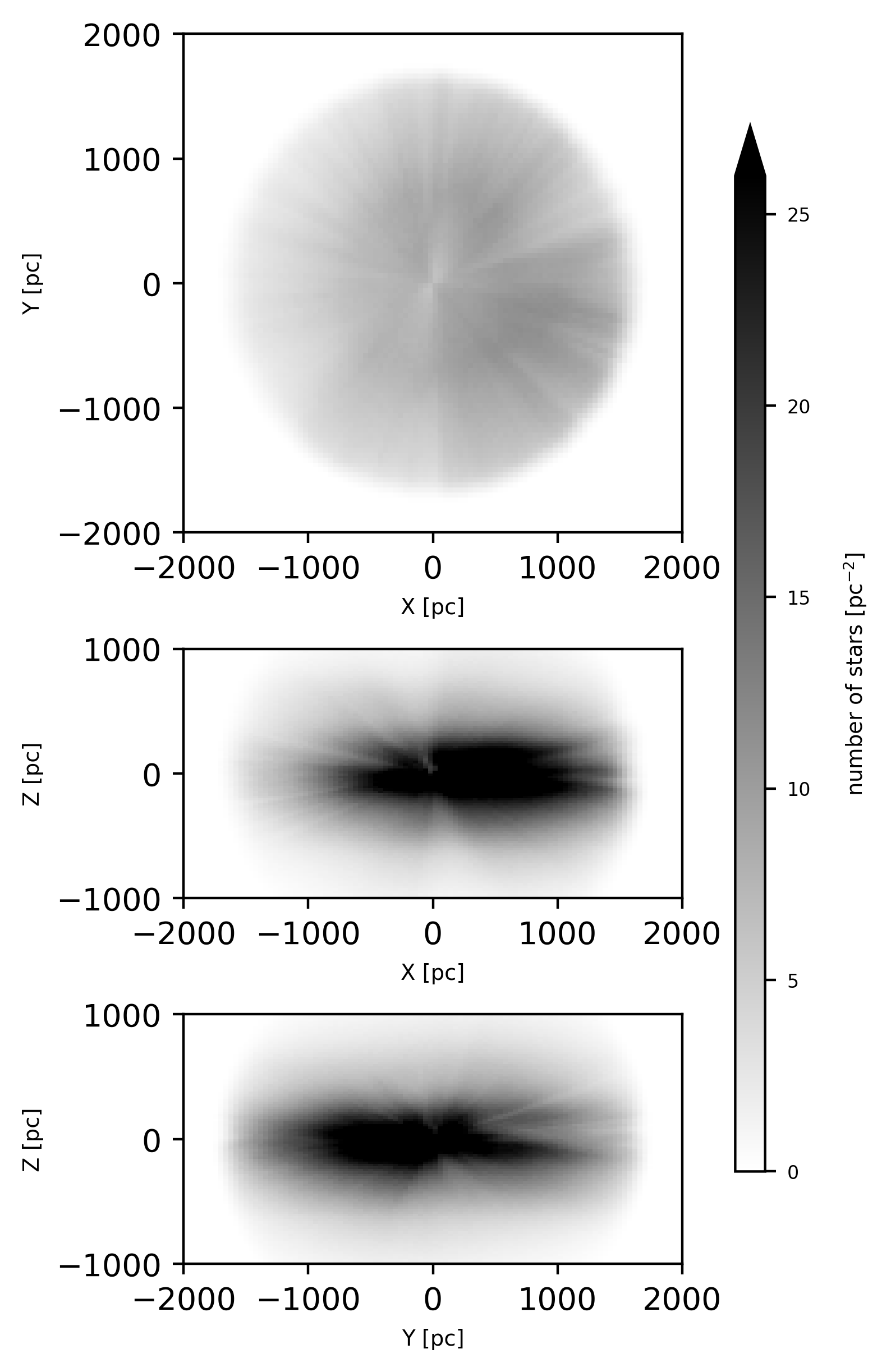
(a) Heliocentric Galactic Cartesian (X, Y, Z) projected histograms.

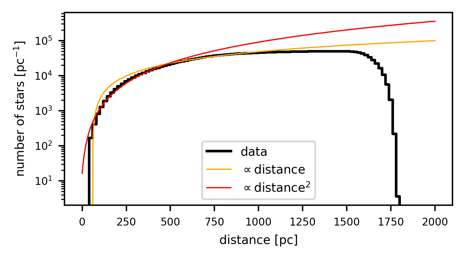
(b) Number of stars as a function of distance.

Figure 1: 2D histograms of the density of stars in heliocentric Galactic Cartesian (X, Y, Z) projections, as well as the density of stars as a function of distance, for the subset of the ZGR23 catalog used in the reconstruction of our 3D dust map. The latter visualization additionally shows a linear growth and a quadratic growth with distance for comparison.

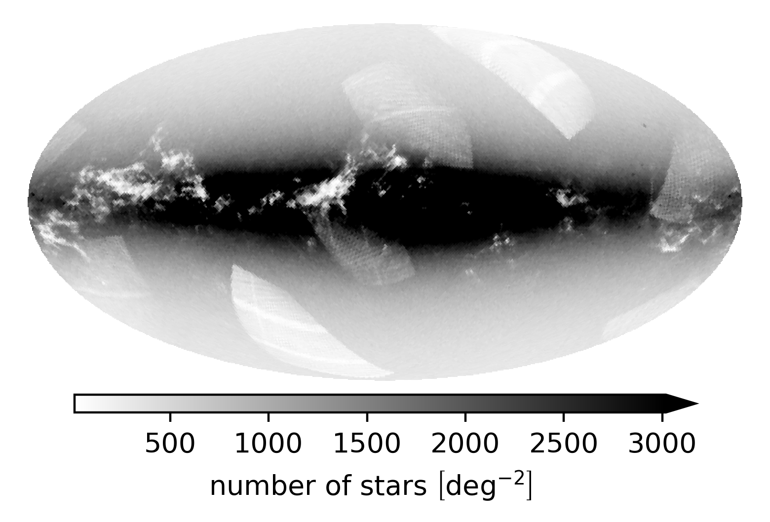
Figure 2: Plane-of-sky distribution of the subset of ZGR23 stars used in the reconstruction of our 3D dust map.

3 Priors

Our quantity of interest is the 3D distribution of differential ZGR23 extinction $\rho$.By definition the differential extinction is positive. Furthermore, we assume it to be spatially smooth. A priori we assume the level of smoothness to be spatially stationary and isotropic.

To reconstruct the 3D volume efficiently, we discretize it in spherical coordinates. Specifically, we discretize our reconstructed volume into HEALPix spheres at logarithmically spaced distances. We adopt an $N_{\text{side}}$ of $256$, corresponding to $786,432$ POS bins. This $N_{\text{side}}$ corresponds to an angular resolution of $14^{\prime}$.For the LOS direction, we adopt $772$ logarithmically spaced distance bins of which $256$ are used for padding. In contrast to reconstructions with linearly-spaced voxels in distance, we are able to probe much larger volumes while maintaining high resolution at nearby distances.

We encode both positivity and smoothness in our model by assuming the differential extinction to be log-normally distributed

$$\rho=\exp{s}$$ (1)

with normally distributed $s$, where $s$ is drawn from a Gaussian process with homogeneous and isotropic correlation kernel $k$. From previous reconstructions of the differential extinction for the Gaia DR2 G-band $A_{G}$ (Leike et al. 2020), we have constraints on the correlation kernel of the logarithm of the differential extinction in a volume around the Sun ($|X|<$370\text{\,}\mathrm{pc}$,\,|Y|<$370\text{\,}\mathrm{pc}$,\,|Z|<$270\text{\,}\mathrm{pc}$$). As part of our prior model we use the inferred $A_{G}$ extinction kernel from Leike et al. (2020). To account for the conversion between the ZGR23 extinction and $A_{G}$ extinction, we add a global multiplicative factor to $s$ in our model.Furthermore, we infer an additive offset in the differential extinction. We place a log-normal prior on the multiplicative parameter and a normal prior on the additive one

We enforce the correlation kernel $k$ using Iterative Charted Refinement (ICR) (Edenhofer et al. 2022). ICR enables us to enforce a kernel on arbitrarily spaced voxels by representing the modeled volume at multiple resolutions. It starts from a very coarse view of our modeled volume. On this coarsest scale, ICR models the GP with learned voxel excitations $\xi_{e}^{(0)}$ and an explicit full kernel covariance matrix. A priori the parameters $\xi_{e}^{(0)}$ are standard normally distributed and coupled according to $k$ via ICR. It then iteratively refines $n_{\text{lvl}}$ times its coarse view of the space with local, fine, a priori standard normally distributed corrections $\xi_{e}^{(1)},\dots,\xi_{e}^{(n_{\text{lvl}})}$ until reaching the desired resolution. In each refinement it uses $n_{\mathrm{csz}}$ neighbors from the previous refinement to refine one coarse pixel into $n_{\mathrm{fsz}}$ fine pixels. See Algorithm 1.

Input: $\xi_{e}^{(0)},\dots,\xi_{e}^{(n_{\mathrm{lvl}})}$

$k,n_{\mathrm{csz}},n_{\mathrm{fsz}}$ Result: $s^{(n_{\mathrm{lvl}})}$

def indices_of_neighbors(index, level, n_neighbors):

       $\dots$

       return indices

      

def cartesian_positions(index, level, n_neighbors):

       $\dots$

       return positions

      

def refine(coarse, fine, pos_coarse, pos_fine, kernel):

       $k_{cc}$ $\leftarrow$ kernel(pos_coarse, pos_coarse)

       $k_{ff}$ $\leftarrow$ kernel(pos_fine, pos_fine)

       $k_{cf}$ $\leftarrow$ kernel(pos_coarse, pos_fine)

       $r$ $\leftarrow$ $k_{cf}^{T}\cdot k_{cc}^{-1}$

       $d$ $\leftarrow$ $k_{ff}-k_{cf}^{T}\cdot k_{cc}^{-1}\cdot k_{cf}$

       $\sqrt{d}$ $\leftarrow$ cholesky($d$)

       return $r$ $\cdot$ coarse + $\sqrt{d}$ $\cdot$ fine

      

$s^{(0)}$ $\leftarrow$ explicit_gp($k$, $\xi_{e}^{(0)}$)

for $l\leftarrow 1$ to $n_{\mathrm{lvl}}$ do

       for $i$ in $\mathrm{ndindex}(\mathrm{shape}(s^{(l-1)}))$ do

             $c$ $\leftarrow$ indices_of_neighbors($i$, $l-1$, $n_{\mathrm{csz}}$)

             $f$ $\leftarrow$ indices_of_neighbors($i$, $l$, $n_{\mathrm{fsz}}$)

             $p_{c}$ $\leftarrow$ cartesian_positions($i$, $l-1$, $n_{\mathrm{csz}}$)

             $p_{f}$ $\leftarrow$ cartesian_positions($i$, $l$, $n_{\mathrm{fsz}}$)

             $s^{i}[f]$ $\leftarrow$ refine($s^{(i-1)}[c]$, $\xi_{e}^{(i)}[f]$, $p_{c}$, $p_{f}$, $k$)

            

       end for

      

end for

Algorithm 1 Pseudocode for ICR creating a GP $s$ from uncorrelated excitations $\left\{\xi_{e}^{(0)},\dots,\xi_{e}^{(n_{\mathrm{lvl}})}\right\}$. Each coarse pixel at location $j$ is iteratively refined to $n_{\mathrm{fsz}}$ fine pixels using $n_{\mathrm{csz}}$ coarse pixel neighbors. The correlation kernel is denoted by $k$. Square brackets after variables and the two functions ndindex and shape denote NumPy-like (Harris et al. 2020) indexing routines. The call explicit_gp refers to an unspecified Gaussian Process model explicitly representing the covariance of $k$ for the pixel positions modeled by $\xi^{(0)}_{e}$.

ICR uses local corrections at varying resolutions and within a refinement assumes the previous iteration to have modeled the GP without error. Both lead to slight errors in representing the kernel. For our use case we encounter errors in representing the kernel of a few percent. We accept these errors as a trade-off that enables the reconstruction to probe larger volumes. We refer to Edenhofer et al. (2022) for a detailed discussion of the kernel approximation errors.

Overall, our model for the prior reads

$$\rho=\exp{\left[\mathrm{scl}(\xi_{\mathrm{scl}})\cdot s\left(\xi_{e}^{(0)},\dots,\xi_{e}^{(n_{\mathrm{lvl}})}\right)+\mathrm{off}(\xi_{\mathrm{off}})\right]},$$ (2)

where we denote the learned multiplicative scaling of $s$ by $\mathrm{scl}$, the learned additive offset by $\mathrm{off}$, and re-expressed both in terms of a priori standard normally distributed parameters $\xi_{\mathrm{scl}}$ and $\xi_{\mathrm{off}}$ respectively. The act of expressing $\mathrm{scl}$, $\mathrm{off}$ and $s$ via parameters with an a priori simpler distribution, here a standard normal distribution, is called re-parameterization. See Rezende & Mohamed (2015) for a detailed discussion on this subject.

4 Likelihood

To construct the likelihood we first need to define how the differential extinction $\rho$ — our quantity of interest — connects to the measured data $\mathcal{D}$. Our data comprises POS position, extinction $\mathcal{D}_{A}$, and parallax $\mathcal{D}_{\omega}$ data. The POS position is in essence without error. The extinction data $\mathcal{D}_{A}=\{A,\sigma_{A}\}$ is in the form of integrated LOS extinctions to stars $A$ and associated uncertainties $\sigma_{A}$ The parallax data $\mathcal{D}_{\omega}=\{\omega,\sigma_{\omega}\}$ similarly is in the form of parallax estimates $\omega$ and uncertainties $\sigma_{\omega}$.

In our model, we focus on the measured extinction $A$ and do not predict parallaxes to stars. Instead, we condition our model on the parallax data $\mathcal{D}_{\omega}$ and split the likelihood into the probability of the measured extinction given the true extinction $a$ and the probability of the true extinction given uncertain parallax information

$$P(A\,|\,\rho,\mathcal{D}_{\omega}) =\int\mathrm{d}{a}\ P(A,a\,|\,\rho,\mathcal{D}_{\omega})$$ (3)

$$=\int\mathrm{d}{a}\ P(A\,|\,a)\cdot P(a\,|\,\rho,\mathcal{D}_{\omega})\ .$$ (4)

The first term of the integrand is constrained by the quality of the extinction measurements and the second by the quality of the parallax measurements.

4.1 Response

The second term in Equation 4 $P(a\,|\,\rho,\mathcal{D}_{\omega})$ can be expressed as the joint probability of extinction and true distance $d$ marginalized over the true distance

$$P(a\,|\,\rho,\mathcal{D}_{\omega}) =\int\mathrm{d}d\ P(a,d\,|\,\rho,\mathcal{D}_{\omega})$$ (5)

$$=\int\mathrm{d}d\ P(a\,|\,\rho,\mathcal{D}_{\omega},d)\cdot P(d\,|\,\rho,\mathcal{D}_{\omega})\ .$$ (6)

We neglect data selection effects, i.e. $a$’s dependence on $\mathcal{D}_{\omega}$ given $d$ and $d$’s dependence on $\rho$ given $\mathcal{D}_{\omega}$, and use that the true extinction $a$ at known distance $d$ is simply the LOS integral of $\rho$ along the LOS to the star from zero to $d$

$$P(a|\rho,\mathcal{D}_{\omega}) =\int\mathrm{d}d\ P(a|\rho,d)\cdot P(d|\mathcal{D}_{\omega})$$ (7)

$$=\int\mathrm{d}d\ \delta\left(a-\underbrace{\int_{0}^{d}\mathrm{d}\tilde{d}\ \rho[\mathrm{POS}](\tilde{d})}_{\coloneqq R^{d}(\rho)}\right)\cdot P(d|\mathcal{D}_{\omega})$$ (8)

with $\rho[\mathrm{POS}]$ the slice of $\rho$ at the POS positions of the stars, $\delta$ the Dirac delta distribution defined by $\int_{-\infty}^{\infty}\mathrm{d}x\ f(x)\delta(x)=f(0)$ for any continuous $f$ with compact support, and $R$ the response which maps from $\rho$ to the domain of the measured extinction.

We approximate $P(a|\rho,\mathcal{D}_{\omega})$ with a normal distribution

$$P(a|\rho,\mathcal{D}_{\omega})\approx\mathcal{G}\left(a|\bar{a},\sigma_{a}^{2}\right)$$ (9)

with mean $\bar{a}$ and standard deviation $\sigma_{a}$ to obtain a tractable expression for Equation 4. The mean extinction $\bar{a}$ is

$$\bar{a} \coloneqq{\langle a\rangle}_{P(a|\rho,\mathcal{D}_{\omega})}$$ (10)

$$=\int\mathrm{d}a\,a\int\mathrm{d}d\ \delta\left(a-R^{d}(\rho)\right)\cdot P(d|\mathcal{D}_{\omega})$$ (11)

$$=\int\int\mathrm{d}a\,\mathrm{d}d\ a\cdot\delta\left(a-R^{d}(\rho)\right)\cdot P(d|\mathcal{D}_{\omega})$$ (12)

$$=\int\mathrm{d}d\ R^{d}(\rho)\cdot P(d|\mathcal{D}_{\omega})$$ (13)

$$={\left\langle R^{d}(\rho)\right\rangle}_{P(d|\mathcal{D}_{\omega})}\ .$$ (14)

Assuming the parallax $\nicefrac{{1}}{{d}}$ is normally distributed, i.e. $P(d|\mathcal{D}_{\omega})=\mathcal{G}\left(\nicefrac{{1}}{{d}}|\omega,\sigma_{\omega}^{2}\right)$ with mean $\omega$ and standard deviation $\sigma_{\omega}$, then

$$\begin{split}{\langle a\rangle}_{P(a|\rho,\mathcal{D}_{\omega})}&={\left\langle R^{d}(\rho)\right\rangle}_{\mathcal{G}(\nicefrac{{1}}{{d}}|\omega,\sigma_{\omega}^{2})}\\ &=\int_{0}^{\infty}\mathrm{d}\tilde{d}\ \rho[\mathrm{POS}](\tilde{d})\cdot\mathrm{sf}_{\mathcal{G}}\left(\nicefrac{{1}}{{\tilde{d}}}|\omega,\sigma_{\omega}^{2}\right)\end{split}$$ (15)

with $\mathrm{sf}_{\mathcal{G}}\left(\nicefrac{{1}}{{d}}|\omega,\sigma_{\omega}^{2}\right)\coloneqq 1-\int_{-\infty}^{\nicefrac{{1}}{{d}}}\mathrm{d}\omega^{\prime}\ \mathcal{G}\left(\omega^{\prime}|\omega,\sigma_{\omega}^{2}\right)$ the survival function of the normal distributed parallax.

The standard deviation $\sigma_{a}$ can be understood as an additional error contribution for marginalizing over the distance. The error depends on the distance uncertainty and the dust along the full LOS

$$\sigma_{a}^{2}\coloneqq{\left\langle{\left(R^{d}(\rho)\right)}^{2}\right\rangle}_{\mathcal{G}\left(\nicefrac{{1}}{{d}}|\omega,\sigma_{\omega}^{2}\right)}-{\langle R^{d}(\rho)\rangle}^{2}_{\mathcal{G}\left(\nicefrac{{1}}{{d}}|\omega,\sigma_{\omega}^{2}\right)}\ .$$ (16)

Evaluating both $\bar{a}$ and $\sigma_{a}^{2}$ is comparatively cheap in a spherical coordinate system since for a discretized sphere $R^{d}(\rho)$ is simply the cumulative sum of $\rho$ along the distance axis weighted by the radial extent of each voxel.

4.2 Likelihood and Joint Probability Density

We assume the measured extinction to be normally distributed around the true extinction $a$. We take the inferred extinction $A$ from the catalog to be the mean of the normal distribution. The accompanying uncertainty $\sigma_{A}$ in the catalog is assumed to be the standard deviation of $P(A\,|\,a)$.

Some stars will have underestimated uncertainties either due to mismodeled intrinsic stellar properties in the inference or bad photometric measurements that were not flagged. We want our model to be able to detect and deselect stars which are in strong disagreement with the rest of the reconstruction. We do so by inferring an additional multiplicative factor per star $n_{\sigma}$ which scales $\sigma_{A}$. A priori, we assume $n_{\sigma}$ to be drawn from a heavy-tailed distribution. Specially, we assume $n_{\sigma}$ to follow an inverse gamma distributed. We again express $n_{\sigma}$ in terms of standard normally distributed parameters $n_{\sigma}(\xi_{\sigma})$ in the inference.

To summarize, our approximate likelihood first introduced in Equation 4, reads

$$\begin{split}&P(A\,|\,\rho,n_{\sigma},\mathcal{D}_{\omega})\\ &\approx\int\mathrm{d}{a}\ \mathcal{G}\left(A\,\left|\,a,{\left(n_{\sigma}\cdot\sigma_{A}\right)}^{2}\right.\right)\cdot\mathcal{G}\left(a\,\left|\,\bar{a}(\rho),\sigma_{a}^{2}(\rho)\right.\right)\end{split}$$ (17)

$$=\mathcal{G}\left(A\,\left|\,\bar{a}(\rho),\left[n_{\sigma}\cdot\sigma_{A}\right]^{2}+\sigma_{a}^{2}(\rho)\right.\right)$$ (18)

The uncertainty in the extinction $\sigma_{A}$ is scaled by $n_{\sigma}$ to deselect outliers and increased by $\sigma_{a}^{2}$ due to marginalizing over the distance uncertainty.

The joint probability density function of data and parameters reads

$$\begin{split}P&(A,\rho(\xi),n_{\sigma}(\xi)|\mathcal{D}_{\omega})\\ &=\ \mathcal{G}\left(A\,\left|\,\bar{a}(\rho(\xi)),\left[n_{\sigma}(\xi)\cdot\sigma_{A}\right]^{2}+\sigma_{a}^{2}(\rho(\xi))\right.\right)\cdot\mathcal{G}\left(\xi\,\left|\,0,1\right.\right)\end{split}$$ (19)

with $\xi$ the vector of all parameters of the model $\left\{\xi_{e}^{(0)},\dots,\xi_{e}^{(n_{\mathrm{lvl}})},\xi_{\mathrm{scl}},\xi_{\mathrm{off}},\xi_{\sigma}\right\}$. The complexity of the prior distributions has been fully absorbed into the transformations $s(\xi)$, $\mathrm{scl}(\xi)$, $\mathrm{off}(\xi)$, and $n_{\sigma}(\xi)$ from the a priori standard normally distributed parameters $\xi$.

Table 1: Parameters of the prior distributions. The parameters $s$, $\mathrm{scl}$, and $\mathrm{off}$ fully determine $\rho$. They are jointly chosen to a prior yield the kernel reconstructed in Leike et al. (2020).

Name	Distribution	Mean	Standard Deviation	Degrees of Freedom
$s$	Normal	$0.0$	Kernel from Leike et al. (2020)	$$786,432$\times 772$
$\mathrm{scl}$	Log-Normal	$1.0$	$0.5$	1
$\mathrm{off}$	Normal	$-6.91\left(\approx\ln 10^{-3}\right)$ prior median extinction from Leike et al. (2020)	$1.0$	1
		Shape Parameter	Scale Parameter
$n_{\sigma}$	Inverse Gamma	$3.0$	$4.0$	# Stars = $53,880,655$

Our priors in terms of non-standard-normal parameters are summarized in Table 1. The priors for $s$, $\mathrm{scl}$, and $\mathrm{off}$ are chosen to a priori yield the kernel reconstructed in Leike et al. (2020). In contrast to Leike et al. (2020), we do not learn a full non-parametric kernel. However, we do infer $\mathrm{scl}$ and $\mathrm{off}$, the scale and zero-mode of the kernel. The prior for $n_{\sigma}$ is chosen such that the inverse gamma distribution has mode $1$ and standard deviation $2$.

5 Posterior Inference

In the previous section we took special care to express our model not only in terms of physical parameters, like the differential extinction density $\rho$, but also in terms of more simple parameters $\xi$. The act of expressing the parameters of the model $\mathrm{scl}$, $\mathrm{off}$, $s$, and $n_{\sigma}$ in terms of a priori standard normal distributed variables $\xi$ is called standardization, a special from of re-parameterization (see Rezende & Mohamed 2015). Effectively we are shifting complexity from the prior to the likelihood. However, both the non-standardized and the standardized formulation of the joint model are equivalent. Standardizing models can lead to better conditioned inference problems as the parameters all vary on the same scales — if the prior is not in conflict with the likelihood. We are going to use an inference scheme that relies on the standardized formulation.

We want to infer the posterior for our standardized model from Equation 19. Directly probing the posterior via sampling methods like Hamiltonian Monte Carlo Hoffman & Gelman (2014) is computationally infeasible. Instead, we use variational inference to approximate the true posterior. Specifically, we use Metric Gaussian Variational Inference (MGVI, Knollmüller & Enßlin 2019). We summarize the main idea behind MGVI in Appendix B. We do not approximate the posterior of the noise inference parameter $n_{\sigma}(\xi_{\sigma})$ via variational inference and instead use only the maximum of the posterior for $\xi_{\sigma}$.

To speed up the inference, we start the reconstruction at a lower resolution ($196,608$ POS bins at $N_{\text{side}}=128$ and $388$ LOS distance bins) and restrict the inference to a subset of stars with a $\geq 2$ sigma chance of being within $600\text{\,}\mathrm{pc}$ and a $\geq 2$ sigma chance of being farther than $40\text{\,}\mathrm{pc}$. We successively increase the distance range of the map up to which stars are incorporated in steps of $300\text{\,}\mathrm{pc}$ from $600\text{\,}\mathrm{pc}$ to $1.8\text{\,}\mathrm{kpc}$. Every time we increase the distance range, we reset the parameters for $n_{\sigma}$. Then, after all data is incorporated, we increase the angular and distance resolution of the reconstruction to the final resolution.

Our data selection deselects stars close to the maximum distance probed (c.f. Figure 1). This effect leads to the outer regions of the map being informed by relatively fewer stars compared to the inner regions. We observe that these regions are prone to producing spurious features. For our final data products we remove the outermost $550\text{\,}\mathrm{pc}$ from the data constrained volume as we observe artifacts aligned with our data incrementation strategy within these regions. We believe $550\text{\,}\mathrm{pc}$ to be a conservative cut but we advise caution when finding structures perfectly aligned with a sphere around the sun at $600\text{\,}\mathrm{pc}$, $900\text{\,}\mathrm{pc}$, or $1200\text{\,}\mathrm{pc}$.

ZGR23 assumes all extinctions to be strictly positive. We neglect this constraint by assuming Gaussian errors which leads to an artificial spike in extinction in the first few voxels in each direction. As we know those regions to be effectively free of dust from previous reconstructions c.f. Leike et al. (2020), we remove the innermost HEALPix spheres until the mean POS differential extinction as a function of distance reaches a local minimum at $69\text{\,}\mathrm{pc}$. We release an additional HEALPix map of integrated extinction out to $69\text{\,}\mathrm{pc}$ from the sun to correct integrated LOS predictions for the removed extinction.

Our inference heavily utilizes derivatives of various components of our model. Derivatives are used for the minimization as well as for the variational approximation of the posterior. Previous models such as Leike & Enßlin (2019); Leike et al. (2020) relied on the Numerical Information Field Theory (NIFTy) package (Selig et al. 2013; Steininger et al. 2017; Arras et al. 2019) and were limited to running on CPUs.

We employ a new framework called NIFTy.re (Edenhofer et al. 2023) for deploying NIFTy models to GPUs. NIFTy.re is part of the NIFTy Python package and internally uses JAX (Bradbury et al. 2018) to run models on the GPU. We are able to speed up the evaluation of the value and gradient of Equation 19 by two orders of magnitude by transitioning from CPUs to GPUs. Our reconstruction ran on a single NVIDIA A100 GPU with 80 GB of memory for about four weeks.

6 Caveats

We believe statistical uncertainties are the dominant source of uncertainty for our reconstruction. However, it is important to also consider sources of systematic uncertainties. Depending on the application, the systematic uncertainties may be more important than the statistical uncertainties. The data that informed the reconstruction, the model with which we inferred it, and the inference procedure all contribute to the model systematic uncertainties.

Naturally, the data themselves is a source of systematic uncertainties (spatially stationary reddening law, mismodeling of binaries, etc,̇ see Zhang et al. 2023) and additionally is known to be incomplete. Given lower stellar densities in heavily obscured regions, volumes of the map behind dense dust clouds are poorly constrained by the data and limits the map’s fidelity, c.f. Figure 2. Thus, we believe our dust reconstruction to be an underestimation of the true extinction toward dense dust clouds. Zucker et al. (2021) also note this effect when comparing the Leike et al. (2020) map with 2D integrated extinction maps based on infrared photometry, finding that the Leike et al. (2020) is not sensitive to regions with $A_{V}\gtrsim 2$ mag.

Our model includes a number of approximations. First, we assume a GP-prior on the logarithmic dust extinction using the kernel from Leike et al. (2020) and additionally only apply it approximately via ICR. Second, we assume $\mathcal{D}_{\omega}$ to be independent of $\mathcal{D}_{A}$. Third, we assume the parallax error to be Gaussian, and fourth, we assume the extinction error to be Gaussian.

For extremely low extinctions the assumption of $A$ being Gaussian is poor due to the positivity prior in the ZGR23 catalog. We correct for this bias towards higher estimated extinction in regions with assumed extremely low true extinctions post-hoc by cutting away the innermost $69\text{\,}\mathrm{pc}$ as described in Section 5 and publish an auxiliary map of integrated extinction out to $69\text{\,}\mathrm{pc}$ from the sun to correct integrated LOS predictions for the removed extinction.

We further release a catalog of the predicted extinctions of our model to all stars that we use for the reconstruction to allow for additional validation work. In Appendix C, we perform a non-exhaustive comparison of our predictions versus the ZGR23 ones. We find that both predictions for the extinction to stars disagree below 50 mmag and above 4 mag (34% more stars than expected have larger respectively smaller extinction prediction compared to ZGR23). See Appendix C for more details.

Furthermore, our posterior inference is an approximation. We assume our approximation of the true posterior accurately captures the intrinsic model uncertainties c.f. (Arras et al. 2022; Leike & Enßlin 2019; Leike et al. 2020; Mertsch & Phan 2023; Roth et al. 2023a; Hutschenreuter et al. 2023; Tsouros et al. 2023; Roth et al. 2023b; Hutschenreuter et al. 2022). However, we do need to worry about structures getting burned in when we increase the maximum distance probed during the inference from $600\text{\,}\mathrm{pc}1800\text{\,}\mathrm{pc}$ in steps of $300\text{\,}\mathrm{pc}$ as described in Section 5. We check the final reconstruction for this effect by comparing it against a larger reconstruction which does not subselect the stars based on their distance during the inference but uses only a small sub-sample of ZGR23 stars with more stringent quality flags. The larger reconstruction which extends out to $2\text{\,}\mathrm{kpc}$ in distance is released as an additional data product. We find no significant differences between both runs. See Appendix D for details on the larger reconstruction.

7 Results

We reconstruct 12 samples (6 antithetically drawn samples) of the 3D dust extinction distribution which each encompasses $607,125,504$ differential extinction voxels. The voxels are arranged on $772$ HEALPix spheres with $N_{\text{side}}=256$ spaced at logarithmically increasing distances. After removing the innermost $<69\text{\,}\mathrm{pc}$ and outermost $>1250\text{\,}\mathrm{pc}$ HEALPix spheres, we are left with $516$ HEALPix spheres. The samples and the posterior mean for the reconstruction are publicly available at https://doi.org/10.5281/zenodo.8187943. We also provide the posterior mean and standard deviation of the reconstruction interpolated to heliocentric Galactic Cartesian Coordinates (X, Y, Z) and Galactic spherical Coordinates ($l$, $b$, $d$) as well as the scripts for the interpolation. Furthermore, the map can be queried via the dustmaps Python package (Green 2018). See Appendix E for further details on using the reconstruction.

The distance resolution in our reconstruction is highest for close-by voxels and decreases further out. Our highest distance resolution is $0.4\text{\,}\mathrm{pc}$ and our lowest distance resolution is $7\text{\,}\mathrm{pc}$.Our angular resolution is $14^{\prime}$ and is independent of the distance.

The reconstruction is in terms of the unitless ZGR23 extinction as defined in Zhang et al. (2023). For visualization purposes we translate the ZGR23 extinction to Johnson’s V-band $\lambda=$540.0\text{\,}\mathrm{nm}$$, i.e. $A_{V}\coloneqq A(V=$540.0\text{\,}\mathrm{nm}$)$. To perform the conversion, we adopt the extinction curve published in ZGR23, and multiply the unitless ZGR23 extinction by a factor of $2.8$. We refer readers to the full extinction curve at https://doi.org/10.5281/zenodo.6674521 from Zhang et al. (2023) for the coefficients needed to translate the extinction to other bands.

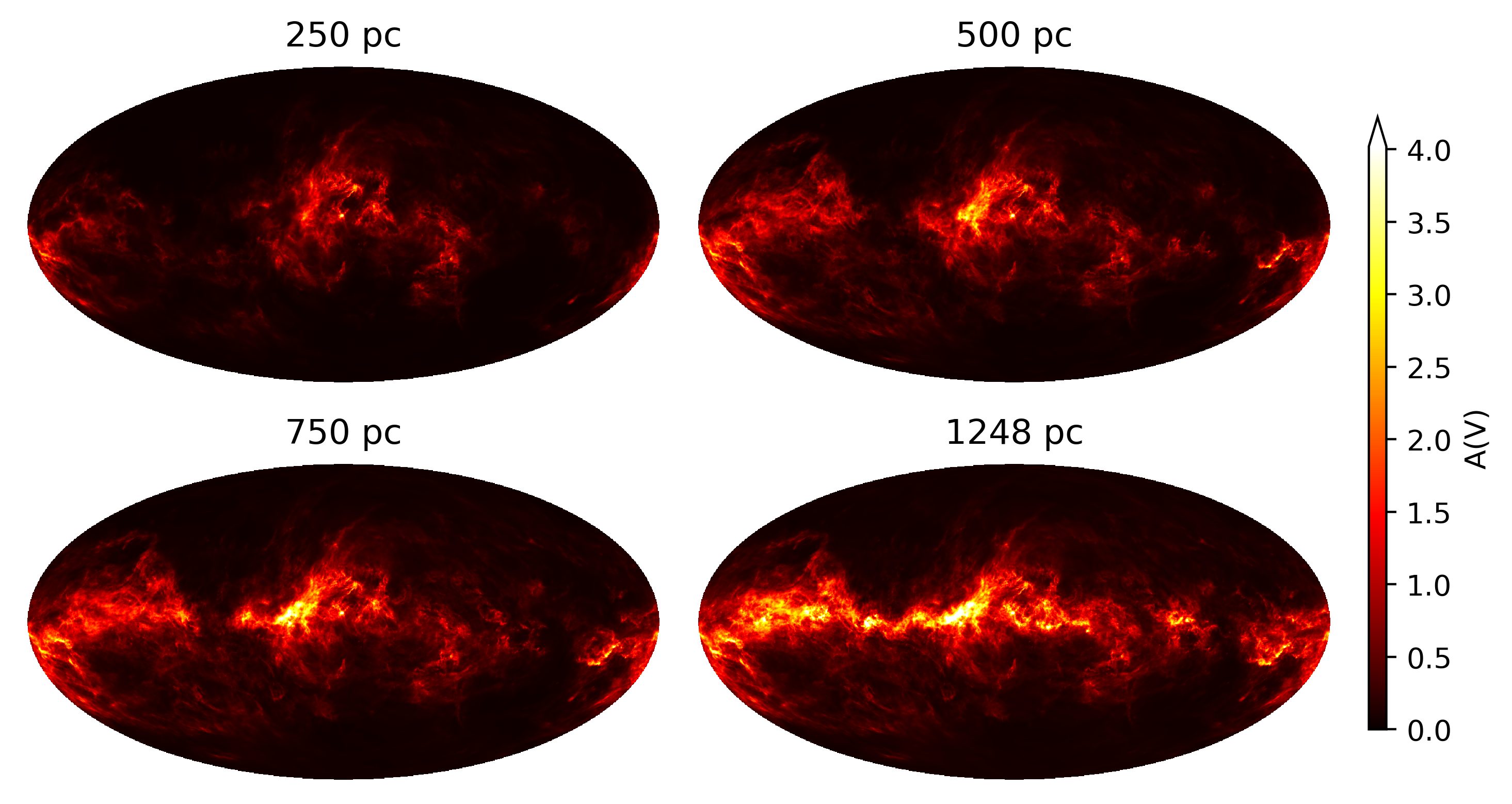
Figure 3: Mollweide projection of the POS integrated $A_{V}$ extinction out to $250\text{\,}\mathrm{pc}$, $500\text{\,}\mathrm{pc}$, $750\text{\,}\mathrm{pc}$, and up to the maximum distance of our map. The colorbar saturates at the $99.9\%$ quantile.

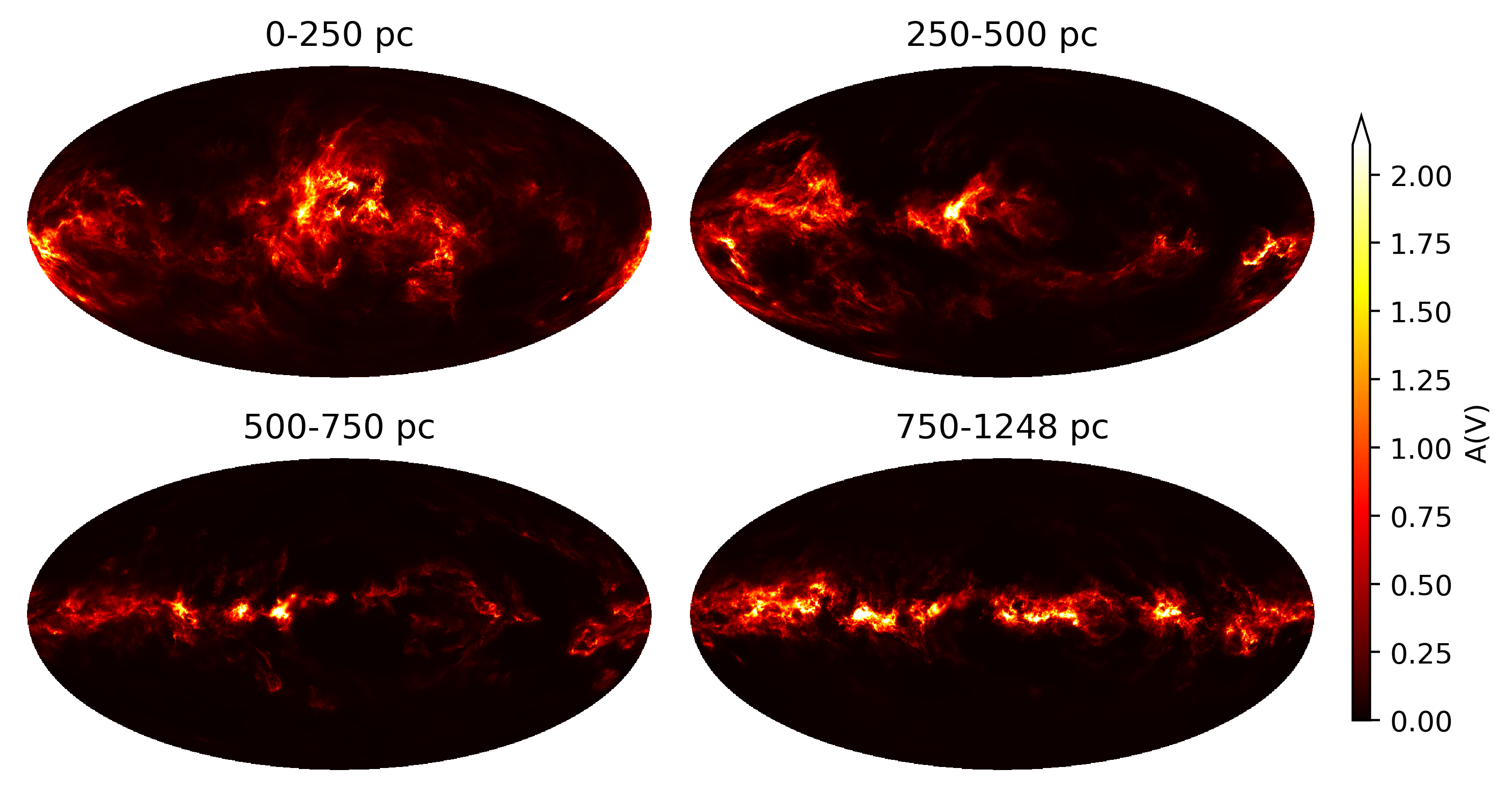
Figure 4: Same as Figure 3 but showing the difference between the integrated extinctions in between distance slices projection on the POS. The colorbar saturates at the $99.9\%$ quantile.

Figure 3 depicts the POS projection of the posterior mean reconstruction integrated out to $250\text{\,}\mathrm{pc}$, $500\text{\,}\mathrm{pc}$, $750\text{\,}\mathrm{pc}$, and up to the end of our sphere. The $A_{V}$ values are in units of magnitudes. We see that higher-latitude features like the Aquila Rift are comparatively close-by while structures in the Galactic plane appear only gradually. Figure 4 shows the difference between the integrated POS projections. We recover well known features of integrated dust but are now able to de-project them.

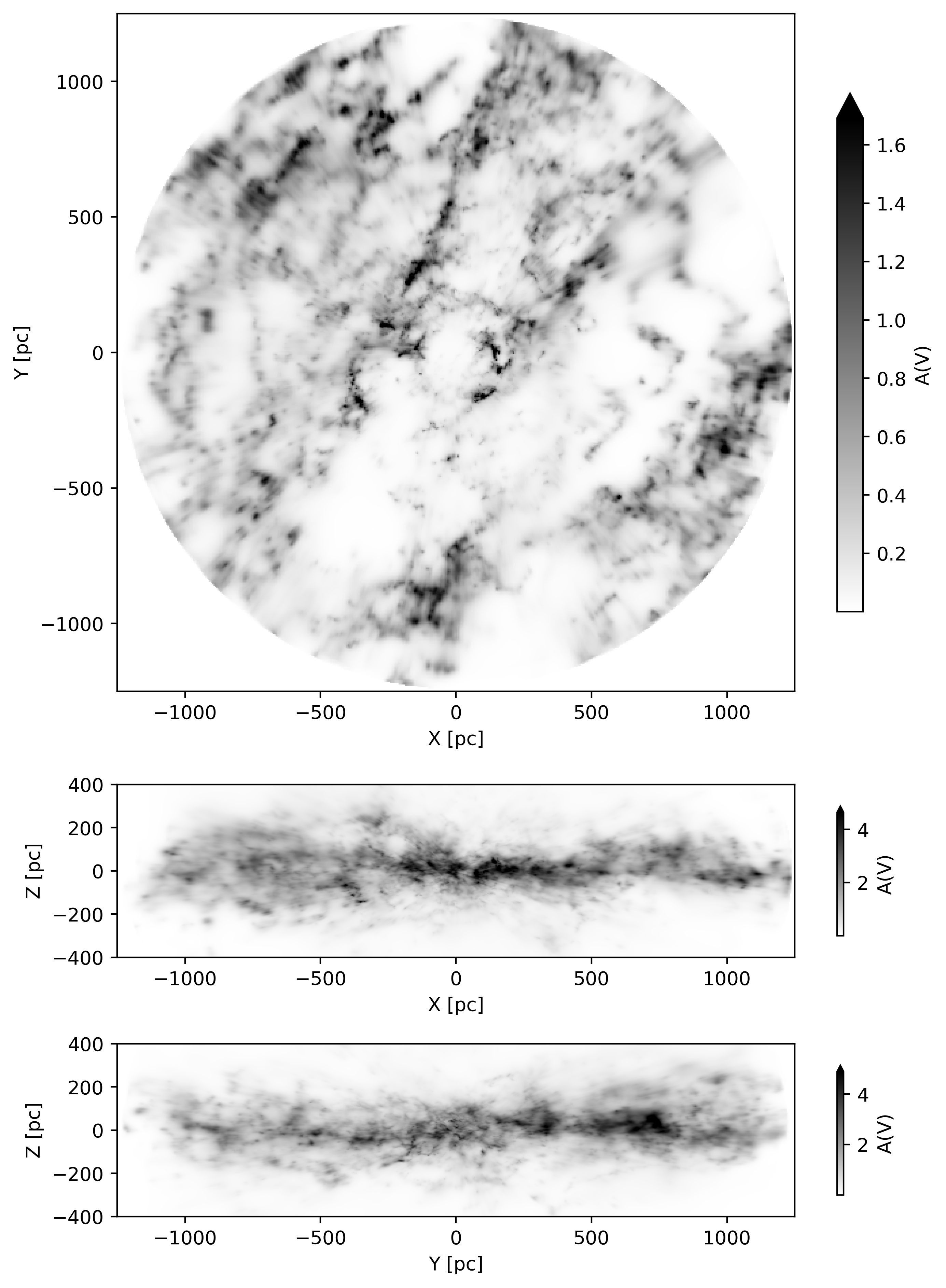
Figure 5: Heliocentric Galactic Cartesian (X, Y, Z) projections of the posterior mean of our 3D dust map in a box with dimensions $$2.5\text{\,}\mathrm{kpc}$\times$2.5\text{\,}\mathrm{kpc}$\times$0.8\text{\,}\mathrm{kpc}$$ centered on the Sun. The colorbar is linear and saturates at the $99.9\%$ quantile. A GIF of the posterior samples is shown at https://faun.rc.fas.harvard.edu/gedenhofer/perm/E+23/21b9_final.gif. A low-resolution 3D interactive version of this figure is available https://faun.rc.fas.harvard.edu/czucker/Paper_Figures/3D_Dust_Edenhofer2023.html.

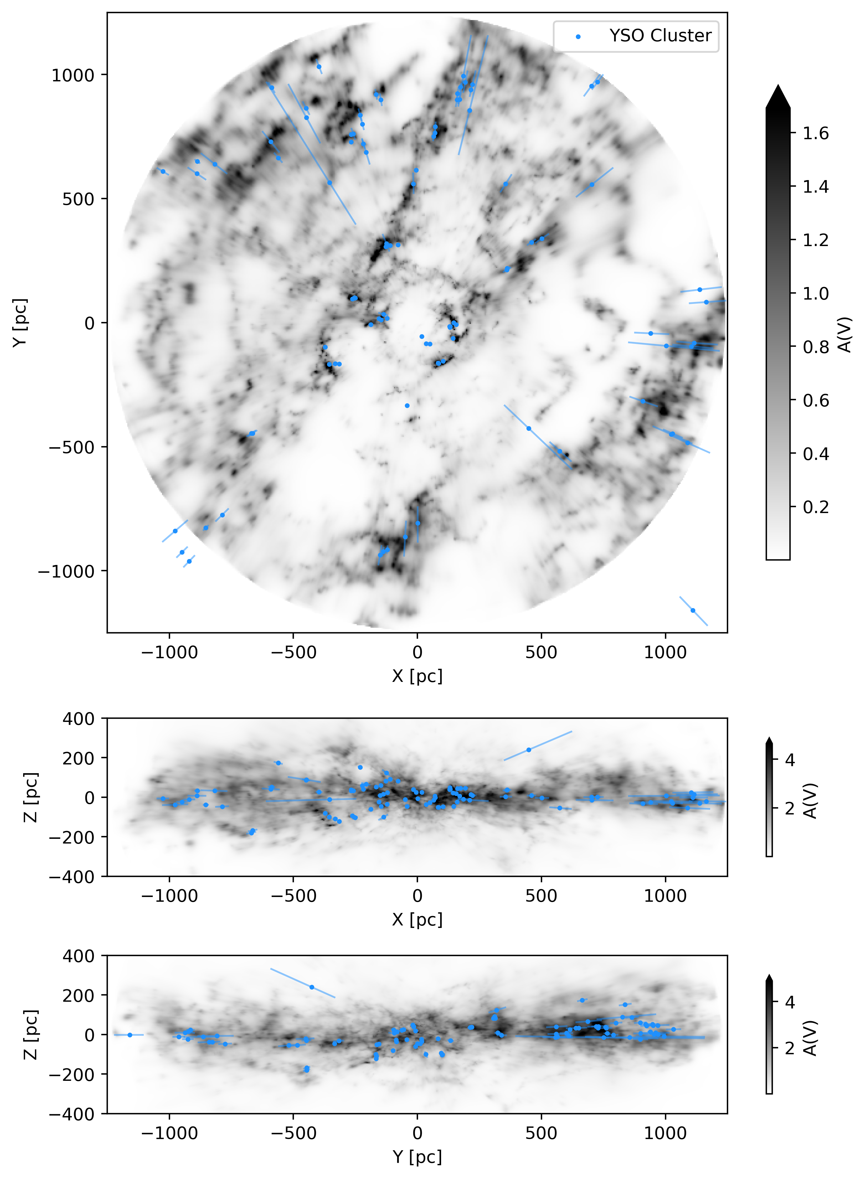
Figure 6: Same as Figure 5 but with a catalog of clusters of young stellar objects (Kuhn 2023) based on Kuhn et al. (2021); Winston et al. (2020); Marton et al. (2022) shown as blue dots on top of the reconstruction and their distance uncertainties shown as extended lines.

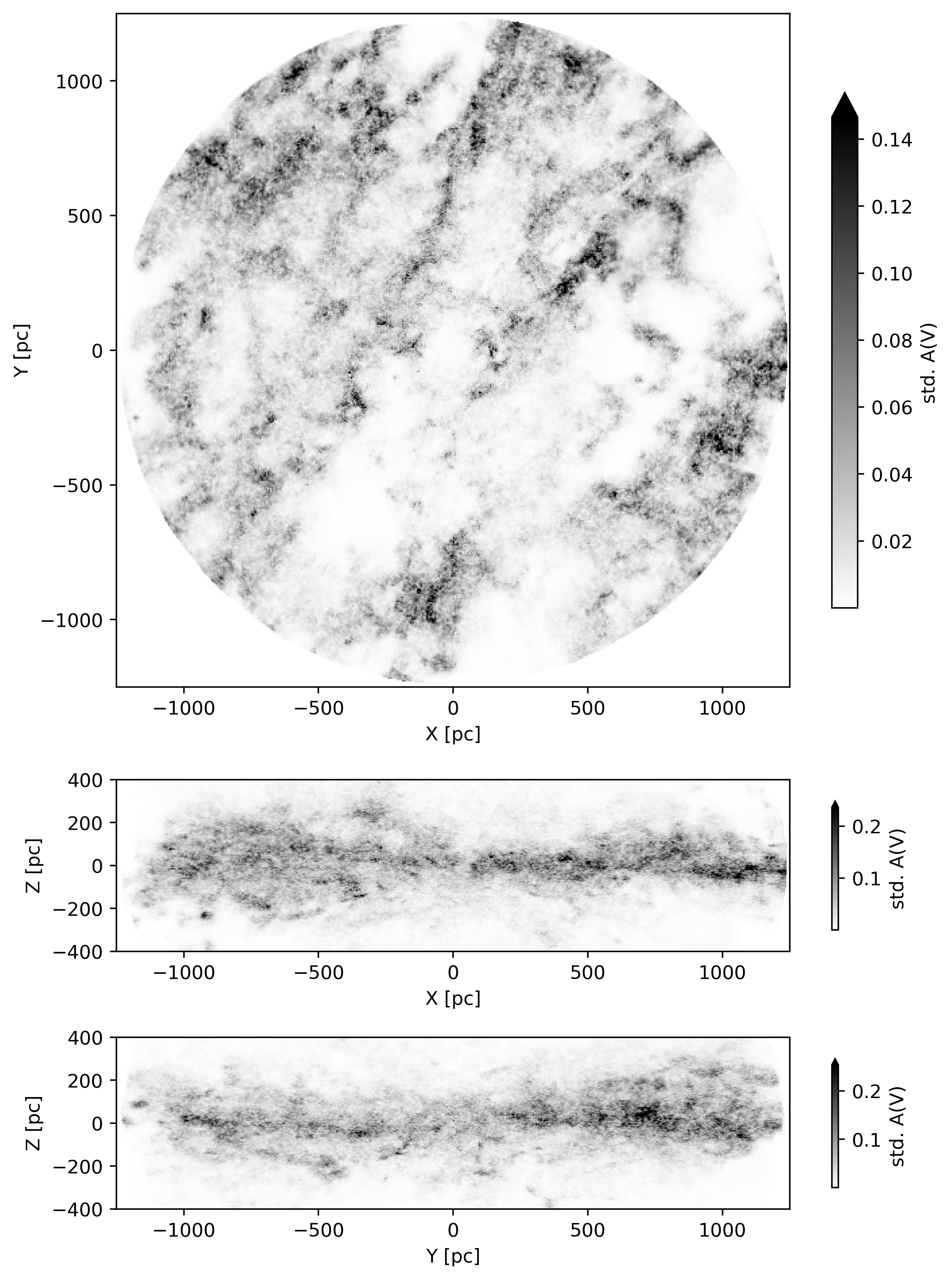
Figure 7: Heliocentric Galactic Cartesian (X, Y, Z) projections of the standard deviation of the reconstructed dust extinction integrated within the box $$2.5\text{\,}\mathrm{kpc}$\times$2.5\text{\,}\mathrm{kpc}$\times$0.8\text{\,}\mathrm{kpc}$$ centered on the Sun. The colorbar is linear and saturates at the $99.9\%$ quantile.

Figure 5 show a bird’s eye (X, Y), side-on (X, Z), and (Y, Z) projection of the posterior mean of our reconstruction in heliocentric Galactic Cartesian coordinates. The image depicts the innermost $$2.5\text{\,}\mathrm{kpc}$\times$2.5\text{\,}\mathrm{kpc}$\times$0.8\text{\,}\mathrm{kpc}$$ around the Sun in $A_{V}$ extinction integrated over $z$ from $-400\text{\,}\mathrm{pc}400\text{\,}\mathrm{pc}$, $y$ in $-1.25\text{\,}\mathrm{kpc}1.25\text{\,}\mathrm{kpc}$, and $x$ in $-1.25\text{\,}\mathrm{kpc}1.25\text{\,}\mathrm{kpc}$, respectively. In Figure 6 we overlay a catalog of clusters of Young Stellar Objects (YSOs) (Kuhn 2023) based on Kuhn et al. (2021); Winston et al. (2020); Marton et al. (2022), which are shown as blue dots. The positions of the YSO clusters visually agree with the positions of dust clouds within the YSO clusters’ reported distance uncertainties. The standard deviation of the reconstruction is shown in Figure 7. It is on the order of $10\%$ of the posterior mean and tends to increase with distance.

The reconstruction has a high dynamic range and reveals faint dust lanes in the reconstructed volume. Small approximately spherical cavities are evident throughout the map. The dust clouds in the reconstruction are compact and only weakly elongated radially. Prominent large-scale features, such as the Radcliffe Wave Alves et al. (2020) and the Split (Lallement et al. 2019), have been resolved at an unprecedented level of detail, previously only accessible for the most nearby dust clouds.

7.1 Comparison to Existing 3D Dust Maps

In this section, we compare our map to other 3D dust maps in the literature. We denote the dust map by Leike et al. (2020) by LGE20, Vergely et al. (2022) by VLC22, Green et al. (2019) by Bayestar19, and Leike et al. (2022) by L+22 in this section. For the purposes of comparison, we show the posterior mean. We release the statistical uncertainties as additional data products, and we strongly advise taking into account these statistical uncertainties for any quantitative analysis. However, the differences between the various 3D dust reconstructions discussed here are systematic differences and are not captured by the reconstructed statistical uncertainties.

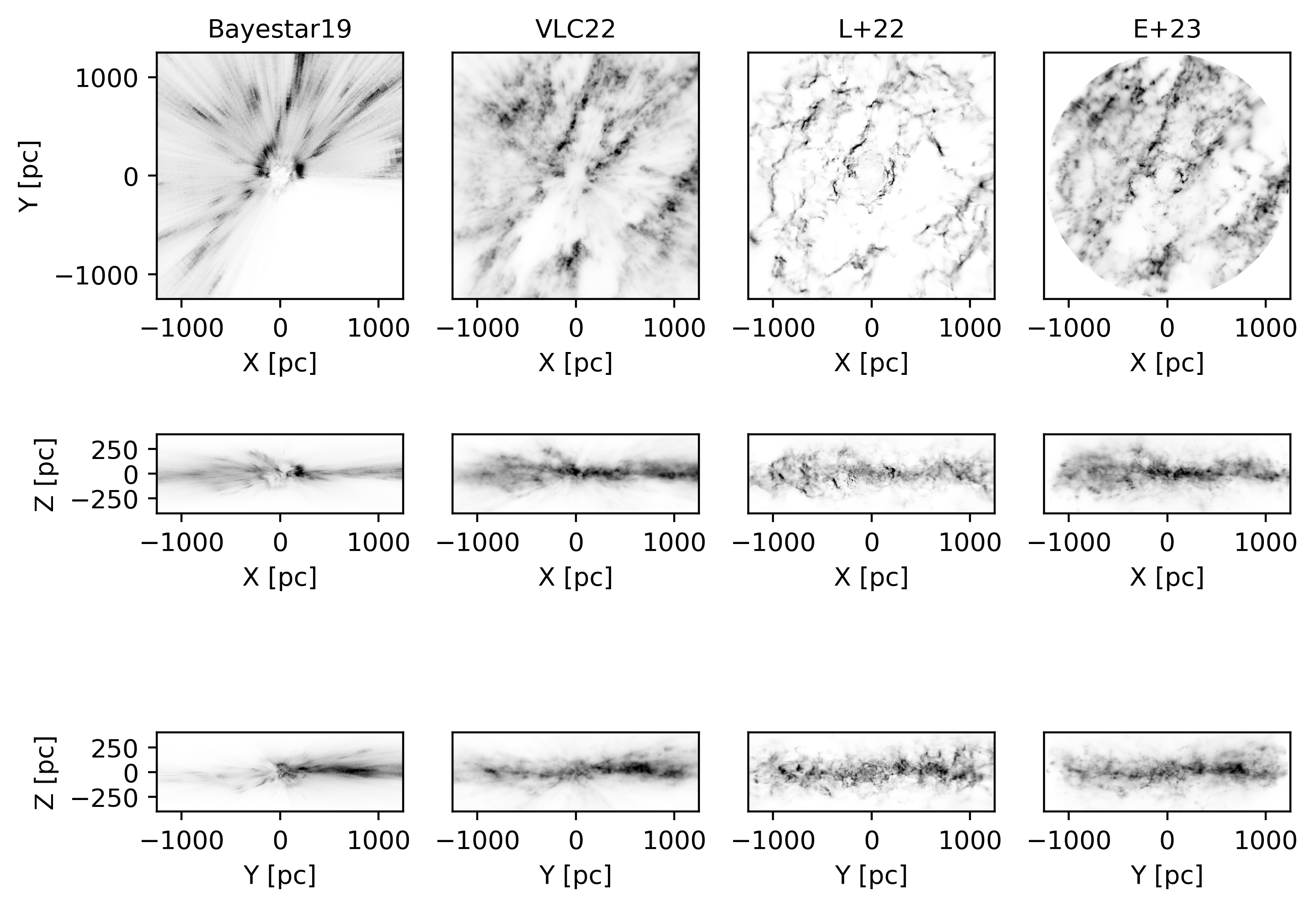
Figure 8: Side-by-side views of the 3D dust maps from Bayestar19, VLC22, L+22 and this work, shown in heliocentric Galactic Cartesian (X, Y, Z) projections. The colorbars are saturated at the $99.9\%$ quantile of the respective reconstruction.

In Figure 8, we show 3D (X, Y, Z) projections of the maps, comparing Bayestar19, VLC22, and this work side-by-side. All four maps agree on the general structure of the distribution of dust.

This work, L+22, and VLC22 have a comparable distance resolution while Bayestar19 only features comparatively few distance bins and more strongly pronounced fingers-of-god. Compared to L+22, we feature more homogenously extended dust clouds and significantly less radial wiggles in the distances to dust clouds. Compared to VLC22, we feature more compact dust clouds, less grainy structures, and a higher dynamic range. Both this work and VLC22 feature dust clouds in a comparable volume around the sun despite the VLC22 map technically extending out further in Galactic heliocentric X and Y.

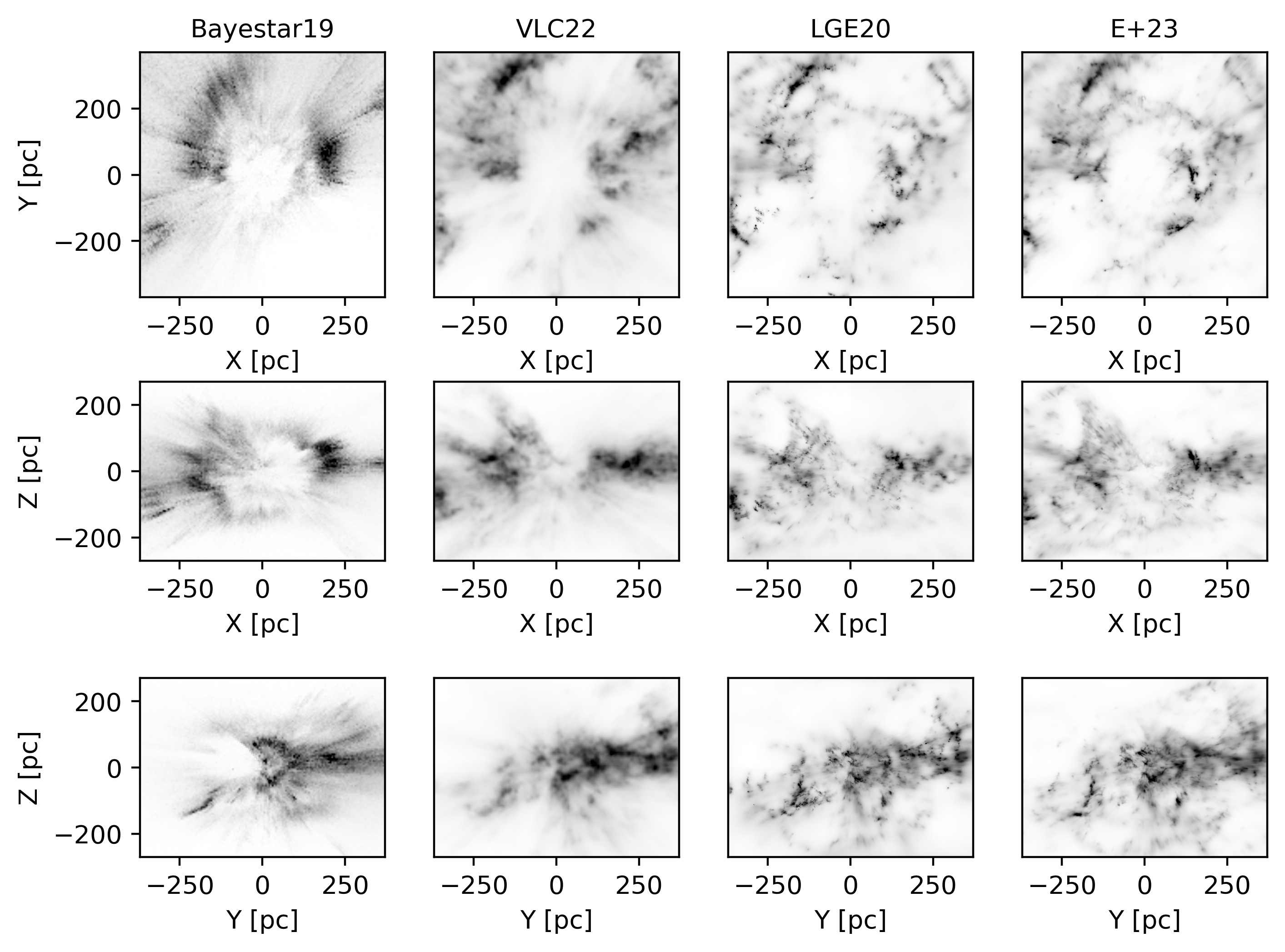
Figure 9: Zoomed-in version of Figure 8 for the volume reconstructed in Leike et al. (2020), now also showing the LGE20 reconstruction for comparison. We leave out L+22 from the comparison because the authors explicitly focus on larger volumes and trade strongly pronounced artifacts in the inner couple hundred parsecs for a larger probed volume. The colorbars are again saturated at the $99.9\%$ quantile of the respective reconstruction.

Figure 9 shows the same projections for the volume reconstructed in the LGE20 map and includes the LGE20 map for comparison. The zoom-in highlights the close similarity between this work and the LGE20 map. All larger structures have direct correspondences in the other map, yet the distances to the structures are slightly different. Furthermore, the LGE20 map appears slightly sharper. The model in LGE20 is very similar to ours but uses fewer approximations. LGE20 also uses compiled data (StarHorse DR2, see Anders et al. 2019). More work is needed to asses the validity of the sharper features in LGE20 not present in this work. The VLC22 map is in good agreement as well but lower resolution. Bayestar19 poorly resolves distances at the scale of the LGE20 map.

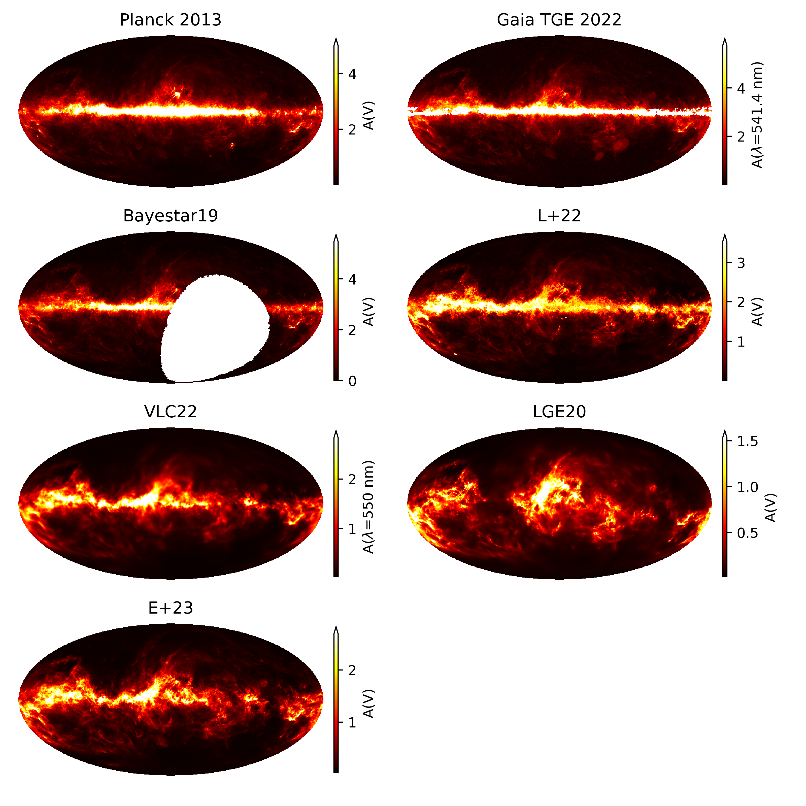
Figure 10: Mollweide projections of total integrated extinction and 3D extinction maps integrated out the maximum distance of the respective map. Bayestar19 reconstructs up to a maximum distance of $63\text{\,}\mathrm{kpc}$ (maximum reliable distance $10\text{\,}\mathrm{kpc}$) and is integrated out to that volume. L+22 reconstructs up to a maximum distance of $16\text{\,}\mathrm{kpc}$ but the authors trust their map only out to $4\text{\,}\mathrm{kpc}$ and we integrate their map only to $4\text{\,}\mathrm{kpc}$. VLC22 reconstructs a heliocentric box of size $$3\text{\,}\mathrm{kpc}$\times$3\text{\,}\mathrm{kpc}$\times$800\text{\,}\mathrm{pc}$$ with $10^{3}\text{\,}{\mathrm{pc}}^{3}$ voxels with at most $<$2.16\text{\,}\mathrm{kpc}$$ in distance and is integrated out to the end of the box. Likewise, LGE20 reconstructs a heliocentric box of size $\rm|X|<$370\text{\,}\mathrm{pc}$,|Y|<$370\text{\,}\mathrm{pc}$,|Z|<$270\text{\,}\mathrm{pc}$$ covering at most $<$590\text{\,}\mathrm{pc}$$ in distance and is integrated out to the end of the box. The colorbars saturate at the respective $99\%$ quantile of the map except for the colorbar of Planck 2013 which saturates at 5 mag for better comparability.

In Figure 10 we compare the POS view of Bayestar19, L+22, VLC22, LGE20 and this work. The respective POS views are integrated out to the maximum distance probed by each map — $<$63\text{\,}\mathrm{kpc}$$ in distance for Bayestar19 (maximum reliable distance $10\text{\,}\mathrm{kpc}$), $<$4\text{\,}\mathrm{kpc}$$ in distance for L+22 (authors trust structures up to $4\text{\,}\mathrm{kpc}$ though the map extends to $16\text{\,}\mathrm{kpc}$), a heliocentric box of size $$3\text{\,}\mathrm{kpc}$\times$3\text{\,}\mathrm{kpc}$\times$800\text{\,}\mathrm{pc}$$ with $10^{3}\text{\,}{\mathrm{pc}}^{3}$ voxels for VLC22 with at most $2.16\text{\,}\mathrm{kpc}$ in distance, and a heliocentric box of size $\rm|X|,|Y|<$370\text{\,}\mathrm{pc}$,|Z|<$270\text{\,}\mathrm{pc}$$ and up to $590\text{\,}\mathrm{pc}$ in distance for LGE20. In addition, we show the Planck 2013 extragalactic dust map (Planck Collaboration et al. 2014) and the Gaia Total Galactic Extinction (TGE) 2022 map (Delchambre et al. 2022).

All maps agree on fine structures at high galactic latitudes but differ in the Galactic plane due to the difference in distance up to which the respective reconstruction extends. 3D dust reconstructions do not probe deep enough into the Galactic plane to fully recover the Planck 2013 extragalactic dust map. Bayestar19 and L+22 probe much deeper than VLC22, LGE20 and this work, yet they do not probe the full column of dust seen in Planck 2013 and Gaia TGE 2022. Both VLC22 and our map probe up to a similar depth while LGE20 only probes dust at much closer distances.

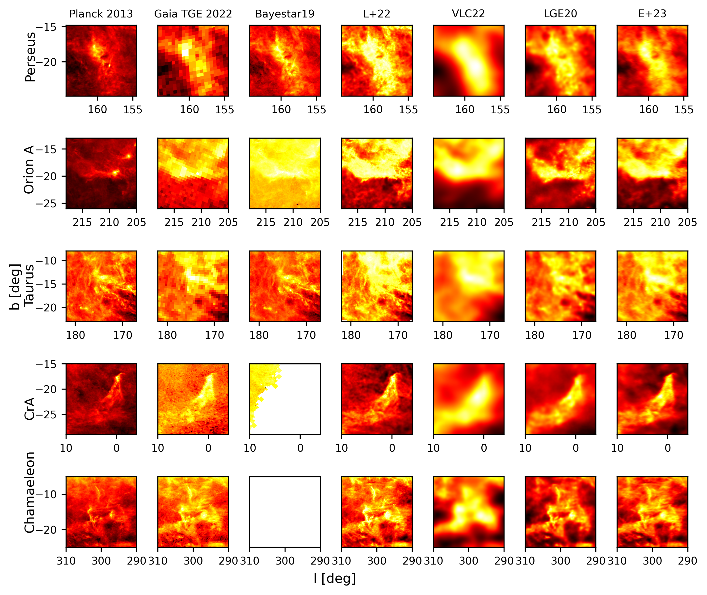
Figure 11: Zoomed-in views toward individual molecular clouds (Perseus, Orion, Taurus, Corona Australis, and Chamaeleon) seen in Figure 10. The colorbars are logarithmic and span the full dynamic range of the selected POS slice in every image. Each row is a separate region and each column a separate reconstruction.

Figure 11 shows a zoom-in comparison of the Perseus, Orion A, Taurus, Corona Australis (CrA), and Chamaeleon molecular clouds, integrated out to the maximum distance of each map ($4\text{\,}\mathrm{kpc}$ for L+22). Among the 3D dust reconstructions, Bayestar19 and L+22 have arguably the highest angular resolution with 3.4’ ($N_{\text{side}}=1024$) and 1.9’ respectively. They resolves the high latitude dust clouds with great detail although L+22 suffers from localized artifacts in patches of the sky. Both LGE20 ($1\text{\,}{\mathrm{pc}}^{3}$ boxes) and this work ($N_{\text{side}}=256$) achieve a comparable angular resolution. The VLC22 reconstruction ($10^{3}\text{\,}{\mathrm{pc}}^{3}$ voxels) is noticeably lower in resolution and does not resolve the cloud substructure on the POS.

8 Conclusions

We present a 3D dust map with a POS and LOS resolution comparable to Leike et al. (2020) that extends out to $1.25\text{\,}\mathrm{kpc}$. We use the distance and extinction estimates of Zhang et al. (2023) which have much lower extinction uncertainties than competing catalogs while probing a similar number of stars. Our reconstruction has an angular resolution of $14^{\prime}$ and a distance resolution of up to $0.4\text{\,}\mathrm{pc}$. We show the map to be in good agreement with existing 3D dust maps and improves upon them in terms of covered volume and spatial resolution. The map is made publicly available at https://doi.org/10.5281/zenodo.8187943 and can also be queried via the dustmaps Python package. We anticipate that the map will be useful for a wide range of applications in studying the distribution of dust and the ISM more broadly.

Appendix A ZGR23 in dust-free Regions

To gauge the reliability of the ZGR23 catalog, we analyze the extinction to stars in dust-free regions, c.f. Leike & Enßlin (2019); Leike et al. (2020). In dust-free regions, we would expect the extinction to be zero within the uncertainties of the catalog. To classify a region as dust-free, we use the Planck dust emission map (Planck Collaboration et al. 2014). A region is said to be dust-free if the Planck $E(B-V)$ map is below or equal to $0.0095\leavevmode\nobreak\ \mathrm{mag}$ or approximately $0.029$ in terms of $A_{V}$.

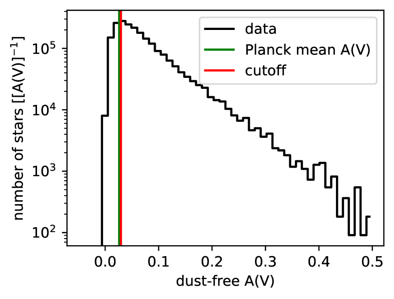
(a) ZGR23 extinction in dust-free regions.

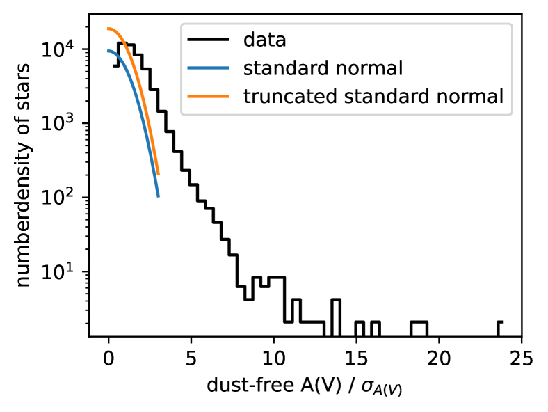
(b) ZGR23 standardized extinction in dust-free regions.

Figure 12: The top plot shows the histogram of the ZGR23 extinctions in dust-free regions translated to $A_{V}$. The mean extinction in dust-free regions based on Planck is shown as a vertical green line and the cutoff value translated to $A_{V}$ for our definition of dust-free is shown in red. The bottom plot shows the same figure from above, but the extinctions are scaled by their accompanying uncertainties. A truncated standard normal distribution and a standard normal distribution are plotted on top. Both ordinates are logarithmic.

The first panel of Figure 12 shows the histogram of ZGR23 extinction to stars with quality_flags$<$8 in dust-free regions translated to $A_{V}$. We see that the histogram of the extinction peaks at the cutoff value and coincides with the mean total extinction as measured by Planck in those regions translated to $A_{V}$. The density of extinction values falls of exponentially after the cutoff value. Overall, the ZGR23 extinction seems to be in good agreement with Planck Collaboration et al. (2014) for dust-free regions.

The second panel of Figure 12 shows the extinction divided by their uncertainties for the stars from Figure 12. The standardized extinctions are centered around unity, indicating that the ZGR23 extinction indeed are offset from zero by about one standard deviation in dust-free regions. This is in agreement with the previous finding that the extinctions are centered around the cutoff value instead of clustering around zero. The width around the center is comparable to a truncated standard normal distribution or a normal distribution. In total, about $1\%$ of the probability mass lies outside the possible range of all ZGR23 extinction with quality_flags<8 if we assume a normal distribution for the extinctions.

Except for outliers far away from the center which can be captured by an outlier model, the ZGR23 catalog seems to be in agreement with POS measurements in dust-free regions and the spread around the cutoff value approximately follows a (truncated) normal distribution. We deem the ZGR23 catalog to be reliable for our purposes and approximate the uncertainties using a normal distribution. We accept the mismodeling of a small fraction of probability mass for a simpler model, see Sections 6 and 5.

Appendix B Metric Gaussian Variational Inference

The variational inference method Metric Gaussian Variational Inference (MGVI) approximates the true posterior $P(\xi\,|\,d)$ with a standard normal distribution in a linearly transformed space in which the posterior more closely resembles a standard normal. Let $Q_{\bar{\xi}}(y\,|\,d)=\mathcal{G}(y(\xi)\,|\,y(\bar{\xi}),\mathbb{1})\left|\frac{\mathrm{d}y}{\mathrm{d}\xi}\right|$ be the approximate posterior and $y(\xi):\xi\mapsto y(\xi)$ the coordinate transformation. In this space the transformed posterior reads $P(\xi(y)\,|\,d)\left|\frac{\mathrm{d}\xi}{\mathrm{d}y}\right|$. We denote the metric of the space in which $P(\xi(y)\,|\,d)\left|\frac{\mathrm{d}\xi}{\mathrm{d}y}\right|$ is “more” standard normal by $M\coloneqq\frac{\mathrm{d}y}{\mathrm{d}\xi}\left(\frac{\mathrm{d}y}{\mathrm{d}\xi}\right)^{\dagger}$. Assuming $y(\xi):\xi\mapsto y(\xi)$ is known, the difficulty lies solely in finding the optimal $\bar{\xi}$ for $Q_{\bar{\xi}}$.

Based on the Fisher information metric and Frequentist statistics, Knollmüller & Enßlin derive a coordinate transformation $y_{\bar{\xi}}(\xi)$ centered on $\bar{\xi}$ that is linear in $\xi$. In Frank et al. (2021), the authors find that a set of Riemannian normal coordinates $y_{\bar{\xi}}(\xi)$ centered on $\bar{\xi}$ are an improved, non-linear estimate of the coordinate transform $y(\xi)\approx y_{\bar{\xi}}(\xi)$. The improvements though come at slightly higher computational costs. We refer the reader to Frank et al. (2021); Frank (2022) for further details on geoVI and its relation to MGVI, the choice of metric, and an analysis of its failure modes. For computational reasons, we use MGVI for our inference.

We start at a random initial position for $\bar{\xi}$ and draw $n_{\text{samples}}$ standard normal samples in the space of $y$. Next, we transform the samples to the space of $\xi$ via $y_{\bar{\xi}}$, our local, linear approximation to $y(\xi)$ at $\bar{\xi}$. We denote the samples in our parameter space by $\{\xi_{1},\dots,\xi_{n_{\text{sampels}}}\}$. Relative to the expansion point $\bar{\xi}$ the samples read $\{\Delta\xi_{1}\coloneqq\xi_{1}-\bar{\xi},\dots,\Delta\xi_{n_{\text{samples}}}\coloneqq\xi_{n_{\text{sampels}}}-\bar{\xi}\}$. The samples $\{\Delta\xi_{1},\dots,\Delta\xi_{n_{\text{samples}}}\}$ around $\bar{\xi}$ provide an empirical, sampled approximation to $Q_{\bar{\xi}}$ which we denote by $\tilde{Q}_{\bar{\xi}}$. We optimize $\bar{\xi}$ of our sampled distribution $\tilde{Q}_{\bar{\xi}}$ by minimizing the variational Kullback–Leibler (KL) divergence between $\tilde{Q}_{\bar{\xi}}$ and the true distribution $P$

$$\bar{\xi}^{\prime}= \operatorname*{arg\,min}_{\bar{\xi}}\mathrm{KL}\left(\tilde{Q}_{\bar{\xi}},\,P(\xi\,|\,d)\right)$$ (20)

$$=\operatorname*{arg\,min}_{\bar{\xi}}{\left\langle\ln{\frac{\tilde{Q}_{\bar{\xi}}}{P(\xi\,|\,d)}}\right\rangle}_{\tilde{Q}_{\bar{\xi}}}$$ (21)

$$=\operatorname*{arg\,min}_{\bar{\xi}}{\left\langle-\ln{P(\xi\,|\,d)}\right\rangle}_{\tilde{Q}_{\bar{\xi}}}$$ (22)

$$=\operatorname*{arg\,min}_{\bar{\xi}}\frac{-1}{n_{\text{samples}}}\sum_{i=1}^{n_{\text{samples}}}\ln{P(\Delta\xi_{i}-\bar{\xi}\,|\,d)}\ .$$ (23)

Note, we keep the relative samples $\{\Delta\xi_{1}\coloneqq\xi_{1}-\bar{\xi},\dots,\Delta\xi_{n_{\text{samples}}}\coloneqq\xi_{n_{\text{sampels}}}-\bar{\xi}\}$ fixed during the optimization and only vary $\bar{\xi}$. Finally, we update the expansion point $\bar{\xi}$ to the new found optimum $\bar{\xi}^{\prime}$.

After the minimization we draw a new set of samples, transform them via a local, linear expansion of $y$, and then minimize again. We repeat the drawing of samples and minimization until we reach a fixed point for $\bar{\xi}$. Algorithm 2 summarizes the algorithmic steps of our variational approximation to the true posterior.

def sample($\xi$, $n_{\text{samples}}$):

       $\dots$

       return $\{\xi_{1},\dots,\xi_{n_{\text{sampels}}}\}$

      

$\bar{\xi}$ $\leftarrow$ …// random init

while $\bar{\xi}$ not converged do

       $\{\xi_{1},\dots,\xi_{n_{\text{sampels}}}\}\leftarrow$ sample($\bar{\xi}$, $n_{\text{samples}}$)

       $\{\Delta\xi_{1},\dots,\Delta\xi_{n_{\text{samples}}}\}\leftarrow\{\xi_{1}-\bar{\xi},\ldots,\xi_{n_{\text{sampels}}}-\bar{\xi}\}$

       $\bar{\xi}\leftarrow\operatorname*{arg\,min}_{\bar{\xi}}\frac{-1}{n_{\text{samples}}}\sum_{i=1}^{n_{\text{samples}}}\ln{P(\Delta\xi_{i}+\bar{\xi}\,|\,d)}$

      

end while

Algorithm 2 Pseudocode for our expansion point variational inference scheme using MGVI.

Appendix C Extinction Catalog

We release a catalog of expected extinction for all stars within the subset of the ZGR23 catalog that we use for our reconstruction (see Section 2). We predict the expected extinction conditional on the known parallax including parallax uncertainties. Our prediction is the best guess of our model for the extinction towards a star but is not necessarily the best guess for the extinction at the mean parallax of the star.

Our extinction predictions (see Sections 3 and 4.1) differ from the extinctions in the ZGR23 catalog by coupling the individual stars via the 3D dust extinction density. By virtue of every star depending on all nearby stars via the prior, our extinction predictions come in the form of joint predictions for all stars. In regions where the 3D dust extinction density is well constraint, the joint predictions to first order factorize into predictions for individual stars, and we can compute expected extinctions for individual stars and their uncertainties.

Our catalog of extinction includes the innermost $69\text{\,}\mathrm{pc}$ from the beginning of our grid and the outer $550\text{\,}\mathrm{pc}$ beyond $1.25\text{\,}\mathrm{kpc}$ that we cut away in the 3D map. We advise caution when analyzing the stars of our catalog within those regions as they might carry additional biases. See Sections 6 and 5 for details on why these regions where removed from the final map.

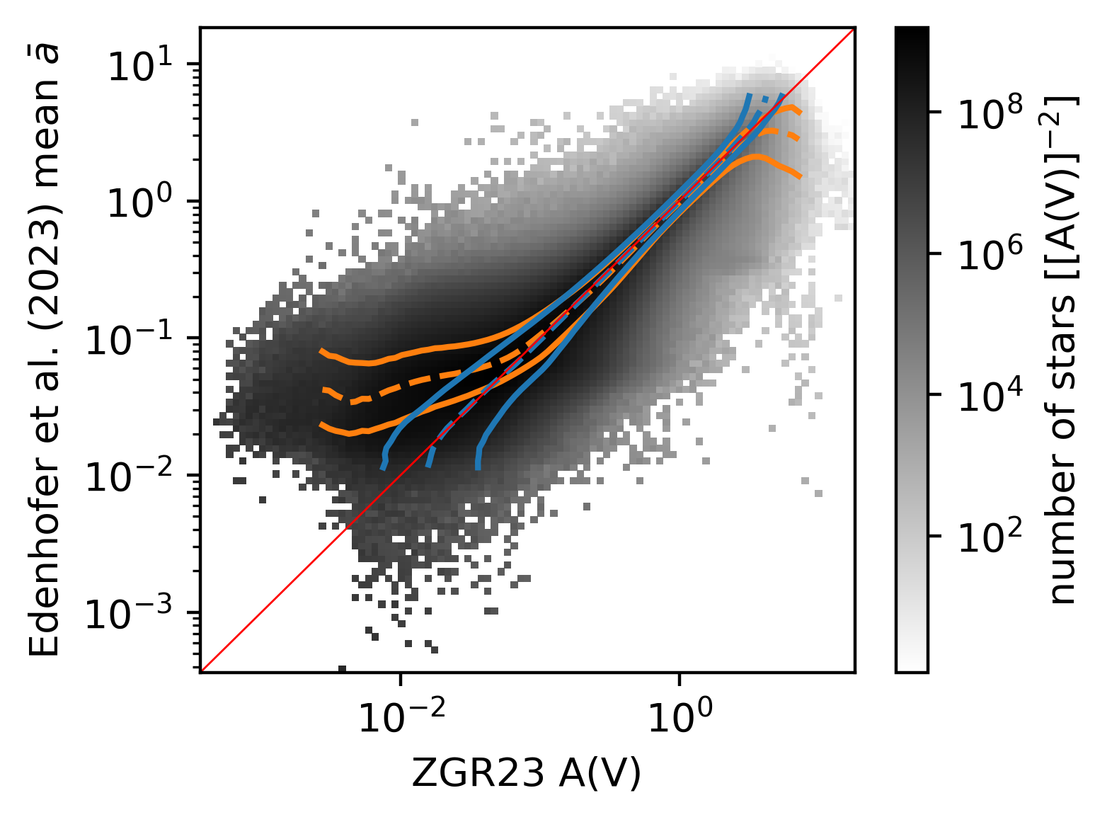
(a) Our extinction prediction versus the ZGR23 extinction.

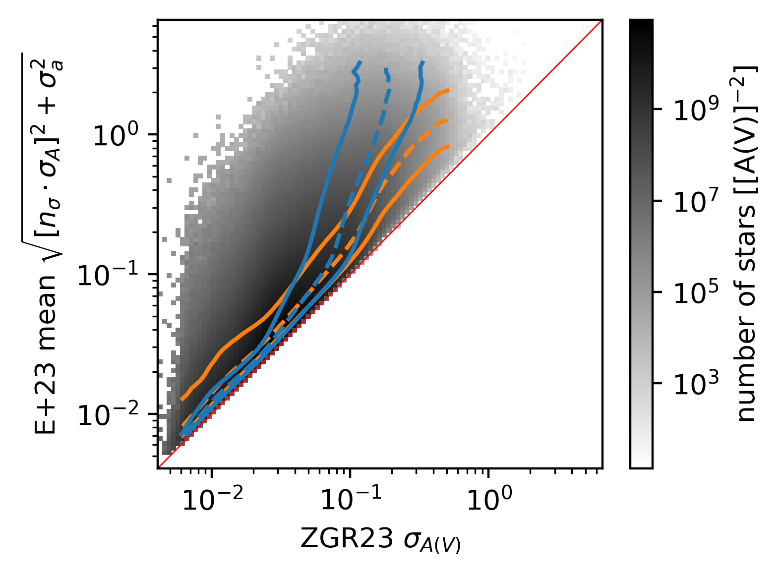
(b) Our inferred uncertainties versus the ZGR23 extinction uncertainties.

Figure 13: The top panel shows our mean posterior extinctions versus the ZGR23 extinctions to stars as 2D histogram. The $16^{\text{th}}$, $50^{\text{th}}$, and $84^{\text{th}}$ quantiles of the ZGR23 extinctions for each bin of our mean extinction are shown as blue lines. The respective quantiles of our predictions in bins of the ZGR23 extinctions are shown as orange lines. The bottom panel shows the same comparison but for our posterior mean predictions for the ZGR23 measurement uncertainties $\sqrt{\left[n_{\sigma}(\xi)\cdot\sigma_{A}\right]^{2}+\sigma_{a}^{2}}$ versus the ZGR23 uncertainties. Note, the predictions for the ZGR23 measurement uncertainties are not the uncertainties of our extinction predictions. See Section 4 and in specific Equation 18 for further details on the quantities shown here. The bisectors are shown in red. The colorbars are logarithmic.

The top panel of Figure 13 compares the ZGR23 extinctions to our mean extinction predictions to stars. Overall, our mean extinctions are in very good agreement with the extinctions in the ZGR23 catalog for the vast majority of stars. However, below 50 mmag and above 4 mag our extinction predictions deviate from the predictions in ZGR23. At any given ZGR23 (respectively our) extinction bin, we would expect half of our (respectively the ZGR23) extinctions to be below and the other half to be above the bisector. At 50 mmag, 34% more stars than expected have higher extinctions than the corresponding extinctions in ZGR23. The difference further widens for lower ZGR23 extinctions. At 4 mag, 34% more stars than expected have lower extinctions than the corresponding extinctions in ZGR23.

The bottom panel of Figure 13 shows our and the ZGR23 extinction uncertainties. Note, our extinction uncertainties are predictions for the measured uncertainties of the ZGR23 catalog $\left[n_{\sigma}(\xi)\cdot\sigma_{A}\right]^{2}+\sigma_{a}^{2}(\rho(\xi))$ and not the uncertainties of our extinction predictions $\mathrm{std}(\bar{a})$, see Section 4. Overall, both uncertainties agree well for the vast majority of stars. At low extinctions uncertainties our uncertainties only marginally inflate the ZGR23 uncertainties. However, at high extinction uncertainties, our predictions cover a larger range, and we find that the ZGR23 significantly underpredicts our extinction uncertainties of stars.

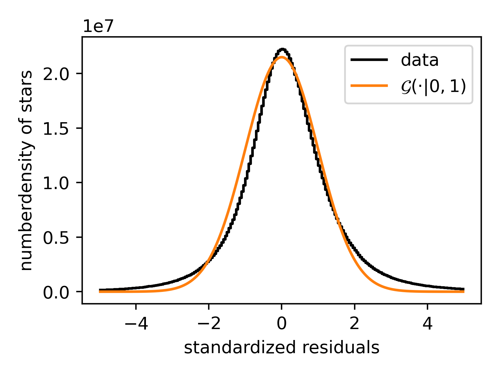
Figure 14: The mean standardized extinctions $(A-\bar{a})/\sqrt{(n_{\sigma}\cdot\sigma_{A})^{2}+\sigma^{2}_{a}}$ (see Section 4 and in specific Equation 18) within the range of $-5$ to $5$.

Figure 14 summarizes the extinctions and the extinction uncertainties of both ZGR23 and our predictions into a single histogram of the mean standardized extinction. The mean standardized residuals follow a standard Gaussian (c.f. Section 4). However, the mean standardized residuals have two slight overdensities at each tail of the Gaussian indicating some outliers are not yet fully captured by our inference of the uncertainties.

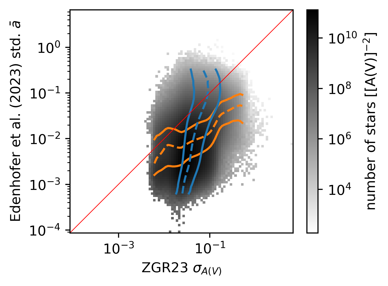
Figure 15: Similar to Figure 13 but for the posterior standard deviation of our extinctions versus the ZGR23 uncertainties. The $16^{\text{th}}$, $50^{\text{th}}$, and $84^{\text{th}}$ quantiles of the ZGR23 uncertainties for each bin of our standard deviation are shown as blue lines. The respective quantiles of our standard deviation in bins of the ZGR23 uncertainties are shown as orange lines. The bisectors are shown in red. The colorbars are logarithmic.

Figure 15 shows the posterior standard deviation of our extinction predictions versus the ZGR23 uncertainties. Our model yields approximately one order in magnitude lower extinction uncertainties than the ZGR23 uncertainties for the vast majority of stars. The effect is less pronounced for low ZGR23 extinction uncertainties.

Our predictions for the extinction to stars theoretically contain more information since we allow for the cross-talk of nearby stars via the 3D distribution of dust and thus might be more accurate. However, the ZGR23 catalog might yield better results in practice because it does not discretize the 3D volume within which the stars reside. By discretizing the modeled volume we can produce contradicting data that in a continuous space is non-contradicting, e.g. by putting highly extincted stars that lie in a dust cloud into the same voxel as less extincted stars that are adjacent to the dust cloud. Overall, both predictions agree very well for stars below between 50 mmag and 4 mag. More work is needed to validate the discrepant predictions at very low and very high extinctions.

Appendix D $2\text{\,}\mathrm{kpc}$ Reconstruction

In Section 5 we describe how we iteratively increase the distance out to our maximum reconstructed distance. We do so to improve the convergence of the reconstruction. We also try naively reconstructing the full volume at once. Using all the available data is computationally prohibitive, so we limit the reconstruction to high quality data using quality_flags==0, $\sigma_{A}\leq 0.04$, and $\nicefrac{{\sigma_{\omega}}}{{\omega}}<0.33$.

We use $\nicefrac{{1}}{{(\omega-\sigma_{\omega})}}<$3\text{\,}\mathrm{kpc}$$ and $\nicefrac{{1}}{{(\omega+\sigma_{\omega})}}>$40\text{\,}\mathrm{pc}$$ to select the stars within a $3\text{\,}\mathrm{kpc}$ sphere. To further speed up the inference we start the inference using at first only a sample of $10\%$, then $20\%$, $45\%$, $67\%$ and finally $100\%$ of the stars. In total, we select $59,334,214$ stars. After the inference, we cut away the outermost $1\text{\,}\mathrm{kpc}$ of the sphere of the data constrained region to avoid degradation effects due to the thinning out of stars at the edge. The overall reconstructed volume after removing the outermost HEALPix spheres extends out to $2\text{\,}\mathrm{kpc}$ in distance.

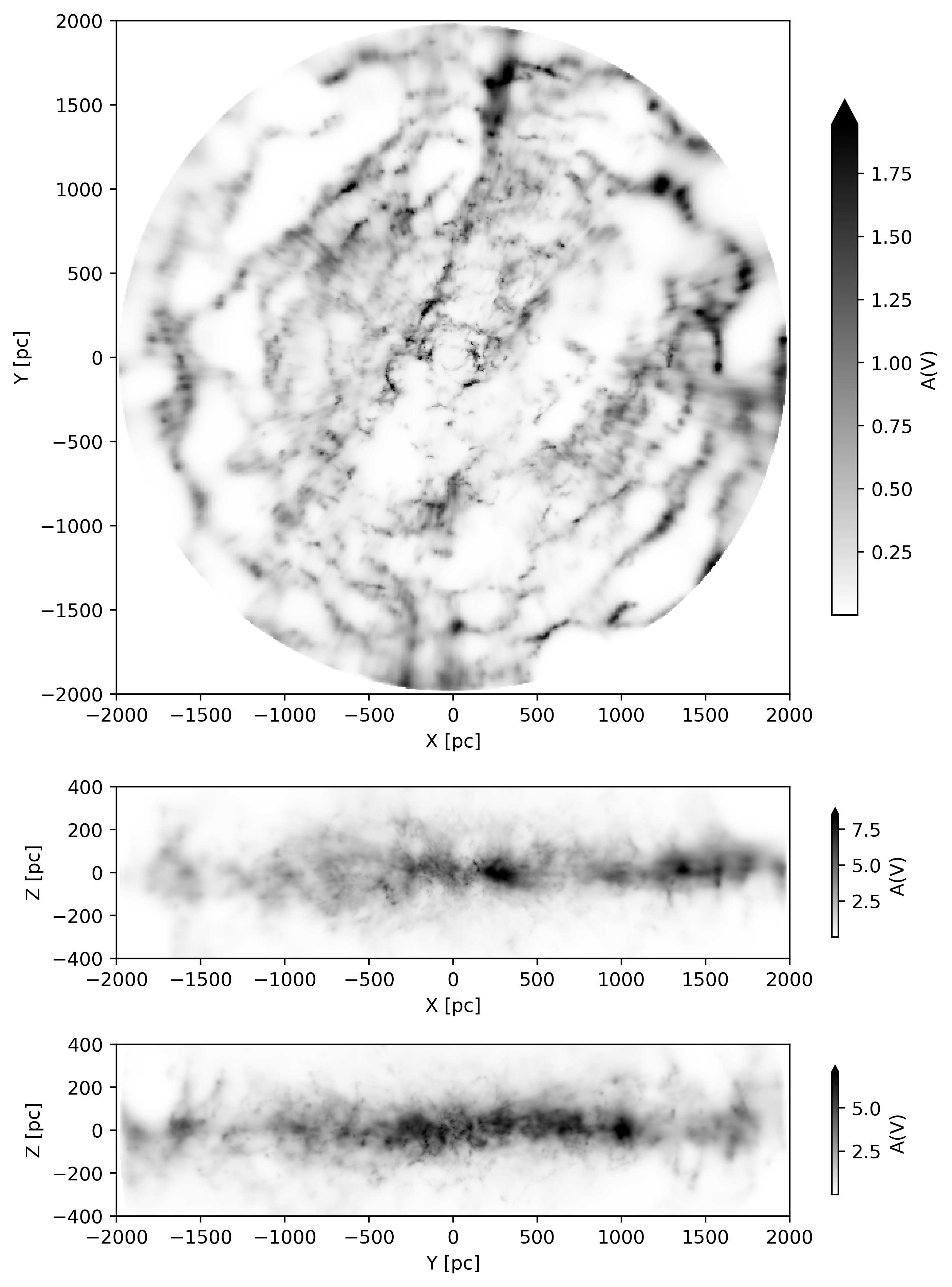
Figure 16: Axis parallel projections of the reconstructed dust extinction in a box of dimensions $$4\text{\,}\mathrm{kpc}$\times$4\text{\,}\mathrm{kpc}$\times$0.8\text{\,}\mathrm{kpc}$$ centered on the Sun. The colorbar is linear and saturates at the $99.9\%$ quantile.

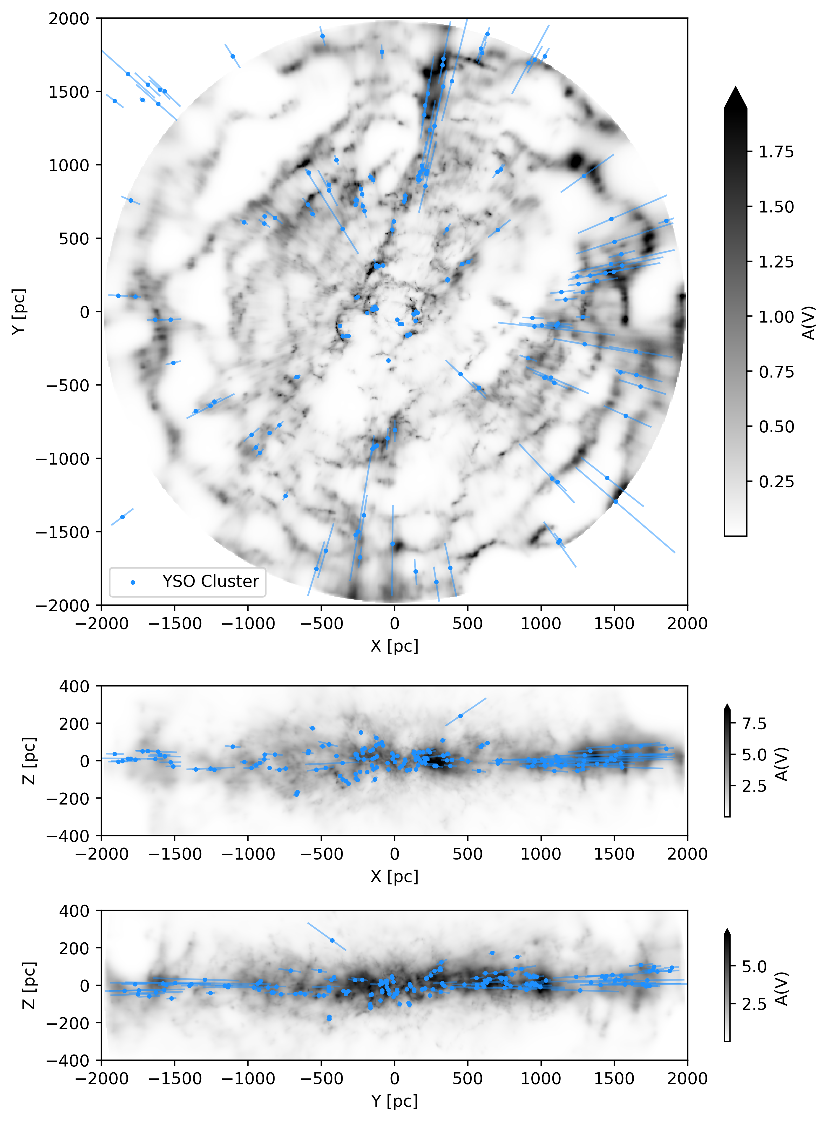
Figure 17: Same as Figure 16 but with a catalog of clusters of young stellar objects (Kuhn 2023) based on Kuhn et al. (2021); Winston et al. (2020); Marton et al. (2022) shown a blue dots on top of the reconstruction and their distance uncertainties shown as extended lines.

The reconstruction is shown in Figure 16 and again in Figure 17 with a catalog of YSO clusters (Kuhn 2023) overlaid on top. It shows the same large scale features as the smaller reconstruction discussed in the main text. The distribution of dense dust clouds is in agreement with the positions of YSO clusters within the distance uncertainties of the YSO clusters. Compared to Figure 5 the reconstruction is less detailed and features more pronounced artifacts.

We use the larger reconstruction to validate the inference of the smaller one. Specifically, we use the larger reconstruction to ensure that structures aligned with or close to the radial boundaries at which we increase the distance of the main reconstruction are independent of the locations at which we increase the distance covered.

We release the larger reconstruction as an additional data product together with the main reconstruction. We advise using the main reconstruction for all regions that fall within its volume. Care should be taken when interpreting small scale features or structures at high distances in the larger reconstruction.

Appendix E Using the Reconstruction

All data products are made publicly available at https://doi.org/10.5281/zenodo.8187943. The data products are stored in the FITS file format. The main data products are the posterior samples of the spatial 3D distribution of dust extinction discretized to HEALPix spheres at logarithmically spaced distances. For convenience, we also provide the posterior mean and standard deviation of the samples of the HEALPix spheres at logarithmically spaced distances.

We additionally interpolate the posterior mean and standard deviation to a Cartesian grid. The interpolation is carried out at a lower resolution using $2^{3}\text{\,}{\mathrm{pc}}^{3}$ voxels to keep the filesize reasonably small. We recommend re-interpolating the map at a higher resolution for the study of individual regions within the map.

We release the interpolation script as part of the data release. Its signature reads interp2box.py [-h] [-o OUTPUT_DIRECTORY] [-b BOX] healpix_path. A box is a string of two tuples separated by two colons. The first tuple specifies the number of voxels along each axis of the box and the second tuple specifies the corners of the box in parsecs in heliocentric coordinates. To interpolate the map to a box with $1051\times 1051\times 351$ voxels of size $\rm|X|,|Y|\leq$2100\text{\,}\mathrm{pc}$$ and $\rm|Z|\leq$700\text{\,}\mathrm{pc}$$, use interp2box.py -b ’(1051,1051,351)::((-2100,2100),(-2100,2100),(-700,700))’ -- mean_and_std_healpix.fits.

In addition, we interpolate the posterior mean and standard deviation to galactic longitude, latitude and distance. The signature of the interpolation script reads interp2lbd.py [-h] [-o OUTPUT_DIRECTORY] [-b BOX] healpix_path. Its behavior is similar to interp2box.py but the box is specified in terms of galactic longitude, latitude and distance in units of degrees, degrees, and parsecs respectively.

Both scripts require the Python packages numpy (Harris et al. 2020), astropy (Astropy Collaboration et al. 2013, 2018, 2022), and healpy (Górski et al. 2005; Zonca et al. 2019). Depending on the number of output voxels, the interpolation can be very memory intensive and computationally expensive.